Approximate String Matching by End-Usersusing Active Learning

Lutz BüchInstitute of Computer Science

Heidelberg University, Germany

lutz.buech@informatik.uni-heidelberg.de

Artur AndrzejakInstitute of Computer Science

Heidelberg University, Germany

artur.andrzejak@informatik.uni-heidelberg.de

ABSTRACT

Identifying approximately identical strings is key for manydata cleaning and data integration processes, including sim-ilarity join and record matching. The accuracy of such taskscrucially depends on appropriate choices of string similaritymeasures and thresholds for the particular dataset. Manualselection of similarity measures and thresholds is infeasible.Other approaches rely on the existence of adequate historicground-truth or massive manual effort.To address this problem, we propose an Active Learning al-gorithm which selects a best performing similarity measurein a given set while optimizing a decision threshold. ActiveLearning minimizes the number of user queries needed toarrive at an appropriate classifier. Queries require only thelabel match/no match, which end users can easily providein their domain. Evaluation on well-known string match-ing benchmark data sets shows that our approach achieveshighly accurate results with a small amount of manual la-beling required.

Categories and Subject Descriptors

H.2.m [Database Management]: Miscellaneous—Datacleaning

Keywords

Active Learning; string similarity; similarity measures; sim-ilarity join; string matching; record matching; deduplication

1. INTRODUCTIONData integration and -cleaning are fields with longstand-

ing importance, that still have space for improvement [19].Many of the tasks in those fields rely on string similar-ity measures, sometimes also a threshold that allows stringmatching. These include record matching [11], similarityjoin [21] and schema matching [17].

Permission to make digital or hard copies of all or part of this work for personal or

classroom use is granted without fee provided that copies are not made or distributed

for profit or commercial advantage and that copies bear this notice and the full citation

on the first page. Copyrights for components of this work owned by others than the

author(s) must be honored. Abstracting with credit is permitted. To copy otherwise, or

republish, to post on servers or to redistribute to lists, requires prior specific permission

and/or a fee. Request permissions from Permissions@acm.org.

CIKM’15, October 19–23, 2015, Melbourne, Australia.

Copyright is held by the owner/author(s). Publication rights licensed to ACM.

ACM 978-1-4503-3794-6/15/10 ...$15.00.

DOI: http://dx.doi.org/10.1145/2806416.2806453.

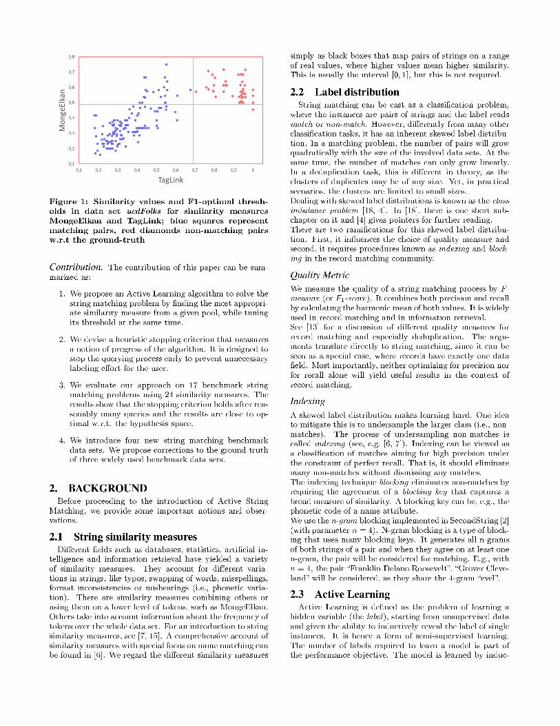
One immediate application of approximate string matchingis similarity join. It is the simple form of record match-ing, where the matching depends only on one key attribute.Differently from a simple join operation, equivalent entitiesfrom both databases may only have similar values in this keyattribute. Specification of a similarity measure and thresh-old define a solution to the similarity join problem. It canthen be reduced to an algorithmic problem, that can be ef-ficiently solved, depending on the similarity measure [21].Record matching relies on similarity measures to computesimilarity values on attribute level [11]. In the Fellegi-Suntermodel, binary comparison vectors are based on similaritymeasures and thresholds for the involved attributes, thatneed to be specified. In many other popular approachessimilarity measures need to be specified, while thresholds forthese functions themselves are not relevant. E.g., in SVM-based approaches, similarity values of several attributes arecombined to a similarity vector. Then, a decision hyperplaneis learned from training data. In decision tree based ap-proaches, several thresholds are learned to constitute predi-cates in logical rules. These thresholds may be inconsistentfor the same attribute and similarity measure across differ-ent predicates used in a tree.Bleiholder et al. point out that the effectiveness of the recordmatching step in data integration is mostly affected by thequality of the similarity measure and the choice of a simi-larity threshold [5]. Figure 1 illustrates that the choice ofa similarity measure can make a huge difference. Here, themeasure TagLink equipped with a suitable threshold canmatch pairs of strings perfectly, while MongeElkan will pro-duce many errors with any threshold.In [11], a large scale comparison of frameworks for recordmatching is done. The authors find that supervised match-ing approaches require less configuration effort and knowl-edge than others, but aspects like the choice of similaritymeasures still have to be determined manually.In this paper we study how to find a suitable similaritymeasure from a given pool and optimize a correspondingthreshold semi-automatically. We propose an Active Learn-ing approach to this problem, in order to minimize humaninput. The user is iteratively queried for the ground-truth,i.e., whether a pair of strings is equivalent or not. A stop-ping criterion suggests that a sufficiently accurate choice canbe done and will terminate this loop. It will return the cho-sen similarity measure along with an appropriately tunedthreshold as the final output.

q

match

q

non-match

0.625

q4

0.667

q2

0.714

q8

0.769

q3

0.667

q9

0.727

q1

Fpred(11, i) = 0.8

q6

0.667

q7

0.75

q5

0.571

q10

0.333

q11

0.0

Figure 3: String pairs qj are aligned according to their similarity value w.r.t to some similarity measure si(similarity values are not shown). Vertical lines indicate possible thresholds, labeled with their respectiveempirical F-measure. The right side of the optimal threshold is highlighted to indicate pairs that are predictedto be matches, the white area (on the left side) non-matches. Diamonds (red) indicate actual matches andsquares (blue) indicate actual non-matches. Pairs without revealed labels are not shown for clarity.

0.571

q5

0.667

q4

0.4

q3

0.5

q1

0.667

q2

0.0

Figure 4: Maximum F1-score values for a measure simay be achieved by multiple candidate thresholds

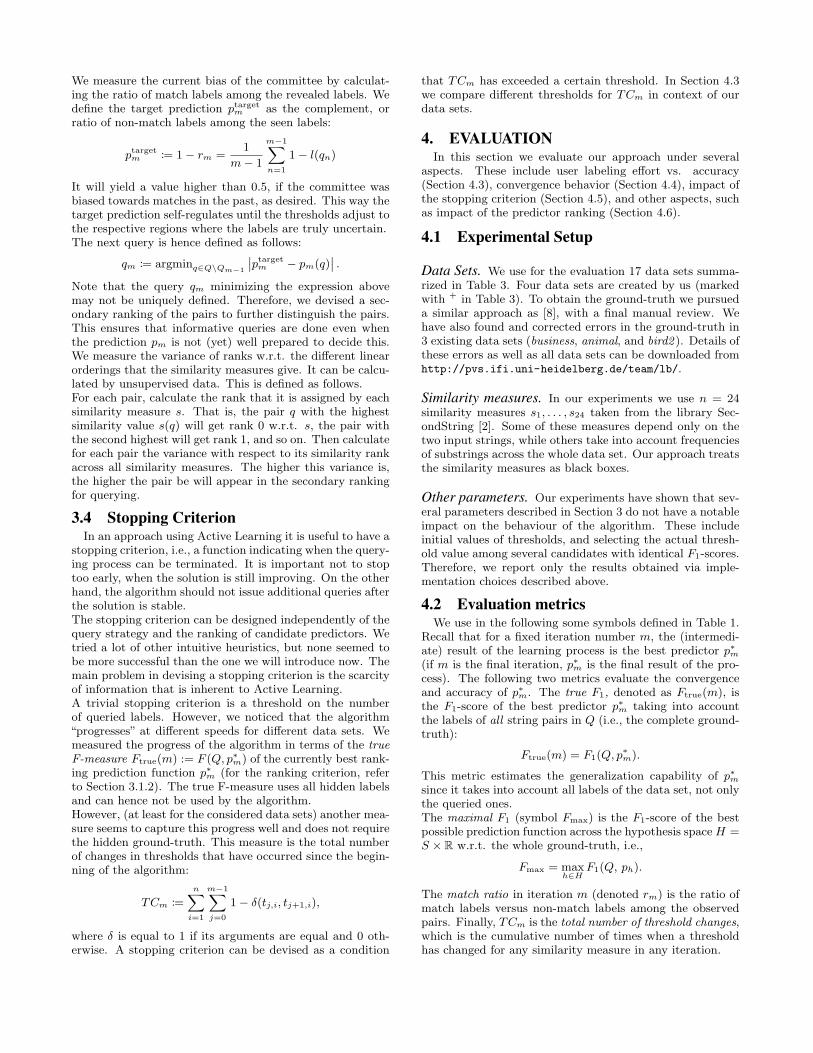
tor defined by Equation (1) for si and a fixed t. We computethe empirical F-measure of p, denoted as F1(Qm, p), basedon the known ground-truth for Qm = {q1, . . . , qm}. Amongall candidate thresholds for si, we consider only those withthe highest empirical F-measure. From these best thresholdcandidates we select only one as a threshold tm,i as describedin Section 3.1.2.The candidate thresholds for si are found as follows. Wefirst compute the values si(q1), . . . , si(qm), that intersect thereal number line in at most m+ 1 intervals. The candidatethresholds are then the arithmetic means of each (closed)interval (and additionally the minimal value si and the max-imal value plus a small constant si+ǫ). Note that any pointwithin one interval yields the same empirical F-measure forthe corresponding candidate predictor.Figure 3 illustrates this. There are 11 labeled pairs q1, . . . , q11that are aligned in a linear ordering, according to their sim-ilarity value as measured by si (increasing from left to right,not shown). The candidates for a new threshold t11,i forsimilarity measure si are the “middles” of each of the 12intervals defined by si(q1), . . . , si(q11). The vertical linesindicate these candidate thresholds; the corresponding em-pirical F-measures are shown in the text labels.The interval defined by si(q1) and si(q6) gives rise to thresh-olds with empirical F-measure of 0.8. This is the best value,and so we use as a threshold tm,i for si the middle of thisinterval. All string pairs q with si(q) ≥ tm,i are now clas-sified by the resulting prediction function p11,i as matches(shaded or red area). Obviously, this prediction functionerrs on some of the queried pairs, namely q3 (false negative)and q7 (false positive).

3.1.2 Ranking of candidate predictors

There are two types of ambiguity when selecting p∗m:(i) for each measure si several candidate thresholds mightlead to the same empirical F-measure, and (ii) after all nthresholds are fixed, several predictors pm,i(q) (i = 1, . . . , n)might achieve the highest value F ∗

pred(m) of the empirical F-measure.Ambiguities of type (i) are illustrated in Figures 3 (thresh-olds of the same interval are equivalent) and 4 (there may

even be different equivalent intervals). We resolve those byselecting as the threshold tm,i for si the middle of the“right-most” interval (i.e., containing the highest similarity values)among all these empirically optimal choices (e.g., betweenq1 and q2 in Figure 4). This choice has little impact on per-formance of the algorithm.Ambiguity in case (ii) occurs since many predictors can havethe same F-measure in a given iteration. As shown in theevaluation (Section 4), this becomes significantly less pro-nounced in later iterations. We devise here a simple sec-ondary heuristic ranking to pick the best from these highestscoring predictors.For each candidate predictor pm,i we inspect the intervalcontaining the selected threshold for pm,i: the lower thenumber of pairs with unrevealed labels in that interval, thehigher the secondary ranking for the predictor. Our heuris-tic intuition is that the spread of these noisy pairs are ex-pected to be more concentrated in good performing hypothe-ses, which leave few intermediate pairs unqueried.

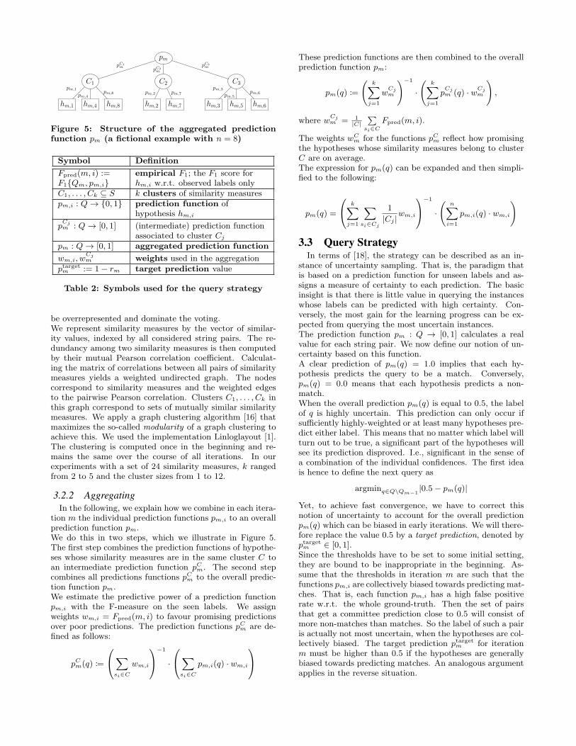
3.2 Aggregated Prediction FunctionIn the following, we introduce an aggregated prediction

function pm that is computed in each iteration m. Thisfunction pm is required by the query strategy described inSection 3.3. We describe how this is done in Sections 3.2.1and 3.2.2. In Section 3.3, we explain how we define the mostuncertain pair based on p.In this paper, we use the term hypothesis as defined in [18].A hypothesis is a classifier (or a configuration that is suffi-cient to identify one), that explains the data by generaliz-ing the ground-truth. In our case, a hypothesis h = (s, t)is determined by a specific similarity measure s from S ={s1, . . . , sn} and a corresponding threshold t ∈ R. Con-sequently, the hypothesis space is H = S × R. RestatingEquation (1), each hypothesis h = (s, t) is assigned a pre-diction function defined by ph(q) = 1 :⇔ s(q) ≥ t. We willwrite hm,i as shorthand for (si, tm,i) and pm,i for phm,i

. Wealso define as Fpred(m, i) := F1{Qm, pm,i} the empirical F1-score for hypothesis hm,i w.r.t. observed labels only (recallthat Qm is the set of already labeled string pairs).

3.2.1 Clustering of Similarity Measures

We account for redundancy among similarity measures byclustering measures that are mutually similar. It is impor-tant to notice about the hypotheses that they are not in-dependent of one another. Some similarity measures maynot even be defined similarly, but produce a very highlycorrelated ordering of pairs. In order to combine their pre-dictions in a meaningful way, it is important to account forthis redundancy. Otherwise some similarity measures might

hm,1 hm,2 hm,3hm,4 hm,5 hm,6hm,7hm,8

C1 C2 C3

pm

pm,1

pm,4pm,8 pm,2 pm,7

pm,3

pm,5pm,6

pC1

mpC2

m

pC3

m

Figure 5: Structure of the aggregated predictionfunction pm (a fictional example with n = 8)

Symbol Definition

Fpred(m, i) :=F1{Qm, pm,i}

empirical F1; the F1 score forhm,i w.r.t. observed labels only

C1, . . . , Ck ⊆ S k clusters of similarity measurespm,i : Q → {0, 1} prediction function of

hypothesis hm,i

pCjm : Q → [0, 1] (intermediate) prediction function

associated to cluster Cj

pm : Q → [0, 1] aggregated prediction function

wm,i, wCjm weights used in the aggregation

ptargetm := 1− rm target prediction value

Table 2: Symbols used for the query strategy

be overrepresented and dominate the voting.We represent similarity measures by the vector of similar-ity values, indexed by all considered string pairs. The re-dundancy among two similarity measures is then computedby their mutual Pearson correlation coefficient. Calculat-ing the matrix of correlations between all pairs of similaritymeasures yields a weighted undirected graph. The nodescorrespond to similarity measures and the weighted edgesto the pairwise Pearson correlation. Clusters C1, . . . , Ck inthis graph correspond to sets of mutually similar similaritymeasures. We apply a graph clustering algorithm [16] thatmaximizes the so-called modularity of a graph clustering toachieve this. We used the implementation Linloglayout [1].The clustering is computed once in the beginning and re-mains the same over the course of all iterations. In ourexperiments with a set of 24 similarity measures, k rangedfrom 2 to 5 and the cluster sizes from 1 to 12.

3.2.2 Aggregating

In the following, we explain how we combine in each itera-tion m the individual prediction functions pm,i to an overallprediction function pm.We do this in two steps, which we illustrate in Figure 5.The first step combines the prediction functions of hypothe-ses whose similarity measures are in the same cluster C toan intermediate prediction function pCm. The second stepcombines all predictions functions pCm to the overall predic-tion function pm.We estimate the predictive power of a prediction functionpm,i with the F-measure on the seen labels. We assignweights wm,i = Fpred(m, i) to favour promising predictionsover poor predictions. The prediction functions pCm are de-fined as follows:

pCm(q) :=

∑

si∈C

wm,i

−1

·

∑

si∈C

pm,i(q) · wm,i

These prediction functions are then combined to the overallprediction function pm:

pm(q) :=

(

k∑

j=1

wCjm

)−1

·

(

k∑

j=1

pCjm (q) · w

Cjm

)

,

where wCjm = 1

|C|

∑

si∈C

Fpred(m, i).

The weights wCm for the functions pCm reflect how promising

the hypotheses whose similarity measures belong to clusterC are on average.The expression for pm(q) can be expanded and then simpli-fied to the following:

pm(q) =

k∑

j=1

∑

si∈Cj

1

|Cj |wm,i

−1

·

(

n∑

i=1

pm,i(q) · wm,i

)

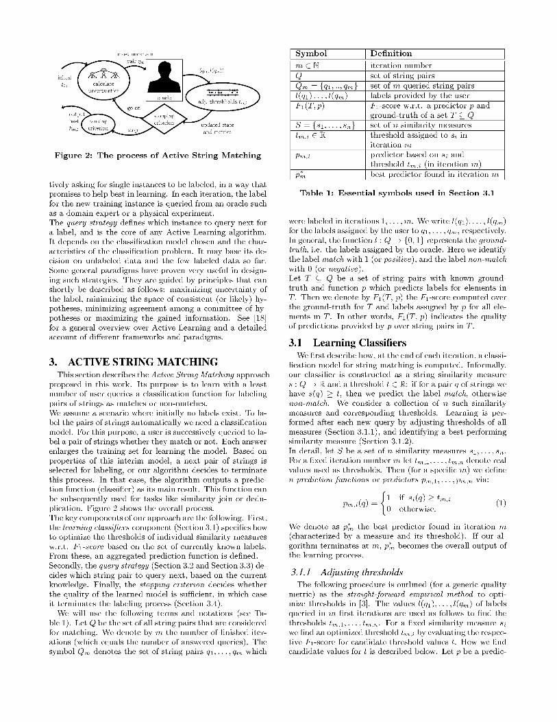
3.3 Query StrategyIn terms of [18], the strategy can be described as an in-

stance of uncertainty sampling. That is, the paradigm thatis based on a prediction function for unseen labels and as-signs a measure of certainty to each prediction. The basicinsight is that there is little value in querying the instanceswhose labels can be predicted with high certainty. Con-versely, the most gain for the learning progress can be ex-pected from querying the most uncertain instances.The prediction function pm : Q → [0, 1] calculates a realvalue for each string pair. We now define our notion of un-certainty based on this function.A clear prediction of pm(q) = 1.0 implies that each hy-pothesis predicts the query to be a match. Conversely,pm(q) = 0.0 means that each hypothesis predicts a non-match.When the overall prediction pm(q) is equal to 0.5, the labelof q is highly uncertain. This prediction can only occur ifsufficiently highly-weighted or at least many hypotheses pre-dict either label. This means that no matter which label willturn out to be true, a significant part of the hypotheses willsee its prediction disproved. I.e., significant in the sense ofa combination of the individual confidences. The first ideais hence to define the next query as

argminq∈Q\Qm−1|0.5− pm(q)|

Yet, to achieve fast convergence, we have to correct thisnotion of uncertainty to account for the overall predictionpm(q) which can be biased in early iterations. We will there-fore replace the value 0.5 by a target prediction, denoted byptargetm ∈ [0, 1].Since the thresholds have to be set to some initial setting,they are bound to be inappropriate in the beginning. As-sume that the thresholds in iteration m are such that thefunctions pm,i are collectively biased towards predicting mat-ches. That is, each function pm,i has a high false positiverate w.r.t. the whole ground-truth. Then the set of pairsthat get a committee prediction close to 0.5 will consist ofmore non-matches than matches. So the label of such a pairis actually not most uncertain, when the hypotheses are col-lectively biased. The target prediction ptargetm for iterationm must be higher than 0.5 if the hypotheses are generallybiased towards predicting matches. An analogous argumentapplies in the reverse situation.

We measure the current bias of the committee by calculat-ing the ratio of match labels among the revealed labels. Wedefine the target prediction ptargetm as the complement, orratio of non-match labels among the seen labels:

ptargetm := 1− rm =1

m− 1

m−1∑

n=1

1− l(qn)

It will yield a value higher than 0.5, if the committee wasbiased towards matches in the past, as desired. This way thetarget prediction self-regulates until the thresholds adjust tothe respective regions where the labels are truly uncertain.The next query is hence defined as follows:

qm := argminq∈Q\Qm−1

∣

∣ptargetm − pm(q)∣

∣ .

Note that the query qm minimizing the expression abovemay not be uniquely defined. Therefore, we devised a sec-ondary ranking of the pairs to further distinguish the pairs.This ensures that informative queries are done even whenthe prediction pm is not (yet) well prepared to decide this.We measure the variance of ranks w.r.t. the different linearorderings that the similarity measures give. It can be calcu-lated by unsupervised data. This is defined as follows.For each pair, calculate the rank that it is assigned by eachsimilarity measure s. That is, the pair q with the highestsimilarity value s(q) will get rank 0 w.r.t. s, the pair withthe second highest will get rank 1, and so on. Then calculatefor each pair the variance with respect to its similarity rankacross all similarity measures. The higher this variance is,the higher the pair be will appear in the secondary rankingfor querying.

3.4 Stopping CriterionIn an approach using Active Learning it is useful to have a

stopping criterion, i.e., a function indicating when the query-ing process can be terminated. It is important not to stoptoo early, when the solution is still improving. On the otherhand, the algorithm should not issue additional queries afterthe solution is stable.The stopping criterion can be designed independently of thequery strategy and the ranking of candidate predictors. Wetried a lot of other intuitive heuristics, but none seemed tobe more successful than the one we will introduce now. Themain problem in devising a stopping criterion is the scarcityof information that is inherent to Active Learning.A trivial stopping criterion is a threshold on the numberof queried labels. However, we noticed that the algorithm“progresses” at different speeds for different data sets. Wemeasured the progress of the algorithm in terms of the trueF-measure Ftrue(m) := F (Q, p∗m) of the currently best rank-ing prediction function p∗m (for the ranking criterion, referto Section 3.1.2). The true F-measure uses all hidden labelsand can hence not be used by the algorithm.However, (at least for the considered data sets) another mea-sure seems to capture this progress well and does not requirethe hidden ground-truth. This measure is the total numberof changes in thresholds that have occurred since the begin-ning of the algorithm:

TCm :=n∑

i=1

m−1∑

j=0

1− δ(tj,i, tj+1,i),

where δ is equal to 1 if its arguments are equal and 0 oth-erwise. A stopping criterion can be devised as a condition

that TCm has exceeded a certain threshold. In Section 4.3we compare different thresholds for TCm in context of ourdata sets.

4. EVALUATIONIn this section we evaluate our approach under several

aspects. These include user labeling effort vs. accuracy(Section 4.3), convergence behavior (Section 4.4), impact ofthe stopping criterion (Section 4.5), and other aspects, suchas impact of the predictor ranking (Section 4.6).

4.1 Experimental Setup

Data Sets. We use for the evaluation 17 data sets summa-rized in Table 3. Four data sets are created by us (markedwith + in Table 3). To obtain the ground-truth we pursueda similar approach as [8], with a final manual review. Wehave also found and corrected errors in the ground-truth in3 existing data sets (business, animal, and bird2 ). Details ofthese errors as well as all data sets can be downloaded fromhttp://pvs.ifi.uni-heidelberg.de/team/lb/.

Similarity measures. In our experiments we use n = 24similarity measures s1, . . . , s24 taken from the library Sec-ondString [2]. Some of these measures depend only on thetwo input strings, while others take into account frequenciesof substrings across the whole data set. Our approach treatsthe similarity measures as black boxes.

Other parameters. Our experiments have shown that sev-eral parameters described in Section 3 do not have a notableimpact on the behaviour of the algorithm. These includeinitial values of thresholds, and selecting the actual thresh-old value among several candidates with identical F1-scores.Therefore, we report only the results obtained via imple-mentation choices described above.

4.2 Evaluation metricsWe use in the following some symbols defined in Table 1.

Recall that for a fixed iteration number m, the (intermedi-ate) result of the learning process is the best predictor p∗m(if m is the final iteration, p∗m is the final result of the pro-cess). The following two metrics evaluate the convergenceand accuracy of p∗m. The true F1, denoted as Ftrue(m), isthe F1-score of the best predictor p∗m taking into accountthe labels of all string pairs in Q (i.e., the complete ground-truth):

Ftrue(m) = F1(Q, p∗m).

This metric estimates the generalization capability of p∗msince it takes into account all labels of the data set, not onlythe queried ones.The maximal F1 (symbol Fmax) is the F1-score of the bestpossible prediction function across the hypothesis spaceH =S × R w.r.t. the whole ground-truth, i.e.,

Fmax = maxh∈H

F1(Q, ph).

The match ratio in iteration m (denoted rm) is the ratio ofmatch labels versus non-match labels among the observedpairs. Finally, TCm is the total number of threshold changes,which is the cumulative number of times when a thresholdhas changed for any similarity measure in any iteration.

Dataset name domain src 1 src 2Original Reduced

pairs match pairs match matches/ pairs

string matching problemsbird3[8] common+scientific animal names 23 15 345 15 25 14 56.00%

USPresidents+ personal names 43 43 1,849 43 173 43 24.86%ucdFolks[14] personal names 45 45 2,025 45 184 45 24.46%

DBconferences+ names of database conferences 54 54 2,963 54 2441 54 2.21%bird1[8] common+scientific animal names 317 20 6,340 19 672 19 2.83%

faoMembers+ country names 194 194 37,636 194 2,633 192 7.29%bird2[8]* common animal names 914 68 62,152 64 4,089 64 1.57%game[8] names of computer games 798 105 83,790 41 4,276 41 0.96%bird4[8] common+scientific animal names 564 155 87,420 155 11,297 155 1.37%park[8] names of (national) parks 393 258 101,394 252 6,767 250 3.69%census[9] synthetic peronal names+addresses 449 392 176,008 329 18,438 326 1.77%

fodorZagrat[20] restaurant names+addr+phone+style 532 331 176,092 114 73,657 112 0.15%

nobelLaureates+ personal names 839 839 703,921 839 27,011 831 3.08%business[8]* company names 1162 962 1,117,844 310 502,316 309 0.06%animal[8]* common animal names 4719 817 3,855,423 178 93,661 175 0.19%

string deduplication problems (single source)UVA[14] institute names 116 6,670 280 2,932 272 9.28%

coraATDV[12] publication references 956 456,490 7,766 453,987 7,766 1.71%

Table 3: Benchmark data sets (ordered by number of pairs) for string matching (upper part) and deduplicationproblems (lower part). Column “Reduced” shows effects of the indexing step. * indicates that ground-truthhas been corrected; italic number of matches means false negatives due to indexing. +indicates new datasets. Summed entries in column “type” indicate concatenated strings of different types.

0

0.2

0.4

0.6

0.8

1

5 10 15 20 25 30 35 40 45 50

Fp

red(m

,1),...F

pre

d(m

,24)

animal

Figure 6: The empirical F1-scores decrease withhigher number of iterations.

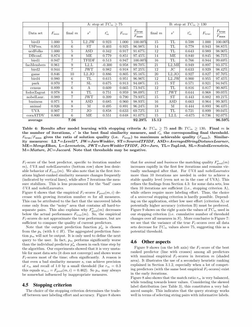
4.3 User effort and predictor accuracyTable 4 reports results for all data sets after learning

prediction models with two different stopping criteria A:TCm ≥ 75 and B: TCm ≥ 130. For criterion A, the averagenumber of queries (or iterations) is 7 and never exceeds 10,which shows that the labeling effort for the user is very low.At the same time, the ratios Ftrue/Fmax of solution quality(i.e. Ftrue) to maximum achievable quality (Fmax, specific toa data set) are high. This indicates that the final matchingprediction functions have been learned well.In case of stopping criterion B, the ratios Ftrue/Fmax are ingeneral higher, but not to a large degree. Also here the aver-

0

0.2

0.4

0.6

0.8

1

40 45 50 55 60 65 70 75 80 85 90 95 100

105

110

115

120

125

130

135

140

Ftr

ue/F

max

TCm

relative performance vs TCm

Figure 7: The ratio of true F1-scores of the best pre-dictor (Ftrue(m)) to Fmax vs. total number of thresh-old changes TCm (each box/whisker plot shows dis-tribution over all data sets).

age number of iterations until stop is relatively low (around15) which implies an acceptable labeling effort. Summariz-ing, we conclude that Active Learning performs very well,and allows minimizing user effort while achieving accurateprediction models.

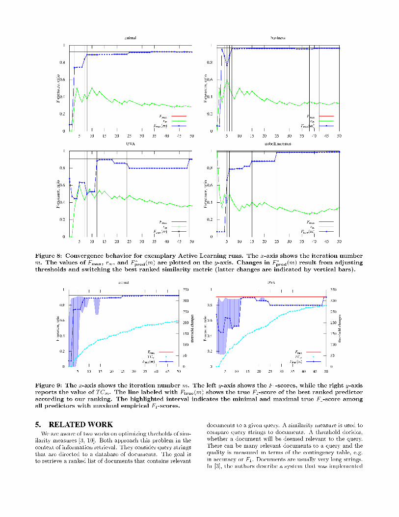
4.4 Convergence behaviorFigure 8 gives more insight into convergence behavior of

some selected representative data sets. While animal andbusiness (top row) illustrate benign changes of Ftrue(m) (the

A: stop at TCm ≥ 75 B: stop at TCm ≥ 130

Data set Fmax final m s∗ t∗m FtrueFtrue

Fmax

final m s∗ t∗m FtrueFtrue

Fmax

bird3 1.000 5 L2 JW 0.923 1.000 100.00% 15 TL 0.598 1.000 100.00%USPres. 0.953 6 ST 0.403 0.925 96.98% 14 TL 0.778 0.943 98.85%ucdFolks 1.000 5 ASD 0.342 0.917 91.67% 12 TL 0.643 0.989 98.90%DBconf. 0.874 8 ME 0.779 0.851 97.45% 14 ME 0.840 0.845 96.75%bird1 0.947 7 TFIDF 0.513 0.947 100.00% 16 TL 0.766 0.944 99.69%

faoMembers 0.961 9 L2 L -0.300 0.958 99.70% 21 L2 ME 0.949 0.897 93.37%bird2 0.944 7 JWT 0.982 0.918 97.25% 12 JC 0.633 0.929 98.42%game 0.846 10 L2 JO 0.886 0.805 95.16% 20 L2 JO 0.927 0.827 97.70%bird4 0.980 6 TL 0.615 0.951 96.96% 12 L2 JW 0.900 0.955 97.45%park 0.970 7 SL 0.675 0.913 94.08% 15 ST 0.571 0.921 94.94%census 0.899 6 A 0.609 0.665 73.94% 12 TL 0.816 0.817 90.80%

fodorZagrat 0.978 8 TL 0.751 0.959 98.09% 17 JWT 0.644 0.968 99.05%nobelLaur. 0.989 7 JWT 0.399 0.790 79.93% 15 ST 0.443 0.882 89.21%business 0.971 8 ASD 0.685 0.960 98.93% 16 ASD 0.663 0.964 99.30%animal 0.926 8 M 0.495 0.891 96.24% 18 M 0.444 0.893 96.43%UVA 0.907 7 JO 0.858 0.633 69.72% 13 TL 0.721 0.899 99.04%

coraATDV 0.800 6 ME 0.551 0.648 81.07% 15 L2 L -0.675 0.736 92.07%average 7.06 92.29% 15.12 96.59%

Table 4: Results after model learning with stopping criteria A: TCm ≥ 75 and B: TCm ≥ 130. Final m isthe number of iterations, s∗ is the best final similarity measure, and t∗m the corresponding final threshold.Ftrue/Fmax gives the ratio of solution quality (i.e. Ftrue) to maximum achievable quality (Fmax). Similar-ity measures: L2 *=Level2*, JW=JaroWinkler, ST=SourcedTFIDF, ASD=AveragedStringDistanceLearner,ME=MongeElkan, L=Levenstein, JWT=JaroWinklerTFIDF, JO=Jaro, TL=TagLink, SL=ScaledLevenstein,M=Mixture, JC=Jaccard. Note that thresholds may be negative.

F1-score of the best predictor, specific to iteration numberm), UVA and nobelLaureates (bottom row) show less desir-able behavior of Ftrue(m). We also note that in the first iter-ations highest-ranked similarity measure changes frequently(indicated by vertical lines), while after 7 iterations the mea-sure stabilizes. This is less pronounced for the “bad” casesUVA and nobelLaureates.Figure 6 shows that the empirical F1-scores Fpred(m, i) de-crease with growing iteration number m for all measures.This can be attributed to the fact that the uncovered labelscome only from the “noisy” area that contains all hard-to-separate pairs. This also explains why F ∗

pred(m) decreasesbelow the actual performance Ftrue(m). So, the empiricalF1-scores do not approximate the true performance, but aresufficient to compare the quality of current predictors.

Note that the output prediction function p∗m is chosenfrom the ph (with h ∈ H). The aggregated prediction func-tion pm will not be output. It is only used to define the nextquery to the user. In fact, pm performs significantly worsethan the individual predictor p∗m chosen in each time step bythe algorithm. Our experiments showed that it is very unsta-ble for most data sets (it does not converge) and shows worseF1-scores most of the time; often significantly. A reason isthat even a bad similarity measure si can achieve precisionof rm and recall of 1.0 by a small threshold (for rm = 0.3this equals wm,i = Fpred(m, i) = 0.462). So pm may alwaysbe somewhat influenced by inappropriate measures.

4.5 Stopping criterionThe choice of the stopping criterion determines the trade-

off between user labeling effort and accuracy. Figure 8 shows

that for animal and business the matching quality F ∗pred(m)

increases rapidly in the first few iterations and remains vir-tually unchanged after that. For UVA and nobelLaureatesmore than 10 iterations are needed in order to achieve astable quality level (even not so in the case of UVA). Thisrefines the findings from Section 4.3: for some data sets, lessthen 10 iterations are sufficient (i.e., stopping criterion A),while others require more labeling effort. Thus, the choiceof a universal stopping criterion is hardly possible. Depend-ing on the application, either low user effort (criterion A) orpotentially higher accuracy (criterion B) must be preferred.Figure 9 shows on the right y-axis the values of TCm used inour stopping criterion (i.e. cumulative number of thresholdchanges over all measures in S). More conclusive is Figure 7:we see that the variance of the true F1-scores over all datasets decrease for TCm values above 75, suggesting this as apotential threshold.

4.6 Other aspectsFigure 9 shows (on the left axis) the F1-score of the best

ranked predictor (line with crosses) among all predictorswith maximal empirical F1-scores in iteration m (shadedarea). It illustrates the use of a secondary heuristic rankingexplained in Section 3.1.2, especially when a lot of compet-ing predictors (with the same best empirical F1-scores) existin the early iterations.Figure 8 also shows that the match ratio rm is very balanced,while tending towards lower values. Considering the skewedlabel distribution (see Table 3), this constitutes a very bal-anced sample. This indicates that the query strategy workswell in terms of selecting string pairs with informative labels.

to take part in a benchmark competition for text retrieval.It is trained online on a stream of queries. They introducescore-distributional threshold optimization, which uses a sta-tistical model to estimate a threshold. The considered simi-larity measure is TFIDF with some preprocessing (like stem-ming and stop word removal). The approach works withany quality metric that is a function of the contingency ta-ble, like the F-measure. The paper outlines the straightfor-ward empirical method to optimize thresholds w.r.t. a givenquality metric, that exhaustively considers all thresholds onthe present training data. The authors dismiss this sim-ple approach, because of its drawbacks in their online prob-lem setting. Most computations involved in their methodcan be updated incrementally. Also, it is able to produce abroad prediction for the threshold with only sparse super-vised data. It is unclear, however, how score-distributionalthreshold optimization performs on only a few samples, sinceit is only evaluated in a very specific online setting. The ap-proach is only evaluated on TFIDF and does not point outany method to compare several similarity measures.The authors of [10] use the straightforward empirical methodw.r.t. optimizing accuracy. Additionally, they formulatea statistical model with a bivariate Gaussian distribution.They show that this model captures the notion of an accu-racy-optimal threshold well. Unfortunately, the evaluationof the optimization is not conclusive. Only one data setwith artificial edit variations is used, and one similarity mea-sure (Levenstein edit distance). The result suggests, thateventually the threshold arrives in the optimal interval. Inthe one experiment this happens close to 40 used samples.One sample corresponds to a ranking list which requires 8labels (relevant or irrelevant to the query). The authorssuggest to use clustering as an unsupervised method to ap-proximate ground-truth to mitigate the labeling effort. Theevaluation does not measure how good the intermediatelyapproximated thresholds are, in terms of any quality met-ric. The sampling method for documents and queries is notdescribed. Finally, a quality metric for similarity measuresis introduced (arithmetic mean of accuracy and the size ofthe output interval of optimized thresholds). This metricis evaluated on eight similarity measures. The results showthat this measure preserves the ranking by accuracy. Hencethe empirical method for threshold optimization can also beused to compare similarity measures in terms of accuracy.

6. CONCLUSIONWe have developed a novel method for finding a simi-

larity measure and an appropriate threshold that work wellspecifically for given data, in order to solve the string match-ing problem. It requires no existing ground-truth and canbe used by end-users. The experimental evaluation showsthat good results can be achieved with only very few itera-tions. We propose two stopping criteria based on a notionof progress. Their thresholds have been determined empir-ically. The result of our proposed algorithm can directlybe used in important applications like similarity join, recordmatching and schema matching.

7. REFERENCES[1] https://code.google.com/p/linloglayout/.

[2] http://secondstring.sourceforge.net/.

[3] A. Arampatzis and A. van Hameran. Thescore-distributional threshold optimization for

adaptive binary classification tasks. In Proceedings ofthe 24th annual international ACM SIGIR conferenceon Research and development in information retrieval,pages 285–293, 2001.

[4] J. Attenberg and F. Provost. Inactive learning?:difficulties employing active learning in practice. ACMSIGKDD Explorations Newsletter, 12(2):36–41, 2011.

[5] J. Bleiholder and F. Naumann. Data fusion. ACMComputing Surveys (CSUR), 41(1):1, 2008.

[6] P. Christen. A comparison of personal name matching:Techniques and practical issues. In ICDM Workshops,2006.

[7] P. Christen. Data Matching. 2012.

[8] W. W. Cohen. Data integration using similarity joinsand a word-based information representationlanguage. ACM Transactions on Information Systems,pages 288–321, July 2000.

[9] W. W. Cohen, P. D. Ravikumar, and S. E. Fienberg.A Comparison of String Distance Metrics forName-Matching Tasks. In S. Kambhampati and C. A.Knoblock, editors, Proceedings of IJCAI Workshop onInformation Integration on the Web, 2003.

[10] R. Da Silva, R. Stasiu, V. M. Orengo, and C. A.Heuser. Measuring quality of similarity functions inapproximate data matching. Journal of Informetrics,1(1):35–46, 2007.

[11] H. Koepcke and E. Rahm. Frameworks for entitymatching: A comparison. Data & KnowledgeEngineering, pages 197–210, Feb. 2010.

[12] A. McCallum, K. Nigam, and L. H. Ungar. Efficientclustering of high-dimensional data sets withapplication to reference matching. In Proceedings ofthe sixth ACM SIGKDD international conference onKnowledge discovery and data mining, 2000.

[13] D. Menestrina, S. E. Whang, and H. Garcia-Molina.Evaluating entity resolution results. Proceedings of theVLDB Endowment, 3(1-2):208–219, 2010.

[14] A. E. Monge, C. Elkan, and others. The FieldMatching Problem: Algorithms and Applications. InKDD, pages 267–270, 1996.

[15] F. Naumann and M. Herschel. An introduction toduplicate detection. Synthesis Lectures on DataManagement, 2(1):1–87, 2010.

[16] A. Noack. Modularity clustering is force-directedlayout. Physical Review E, 79(2), 2009.

[17] E. Rahm and P. A. Bernstein. A survey of approachesto automatic schema matching. the VLDB Journal,10(4):334–350, 2001.

[18] B. Settles. Active Learning. 2012.

[19] M. Stonebraker, I. F. Ilyas, S. Zdonik, G. Beskales,and A. Pagan. Data Curation at Scale: The DataTamer System. 6th Biennial Conference on InnovativeData Systems Research, 2013.

[20] S. Tejada, C. A. Knoblock, and S. Minton. LearningObject Identification Rules for InformationIntegration. Information Systems, 2001.

[21] C. Xiao, W. Wang, X. Lin, J. X. Yu, and G. Wang.Efficient similarity joins for near-duplicate detection.ACM Transactions on Database Systems (TODS),36(3):15, 2011.