approximate shortest path queries using voronoi …) 13:)))))

Approximate Shortest Path Queries Using Voronoi Duals∗

Shinichi Honiden Michael E. Houle Christian Sommer† Martin Wolff

November 13, 2009

Abstract

We propose an approximation method to answer point-to-point shortest path queries inundirected edge-weighted graphs, based on random sampling and Voronoi duals. We computea simplification of the graph by selecting nodes independently at random with probability p.Edges are generated as the Voronoi dual of the original graph, using the selected nodes asVoronoi sites. This overlay graph allows for fast computation of approximate shortest paths forgeneral, undirected graphs. The time–quality tradeoff decision can be made at query time. Weprovide bounds on the approximation ratio of the path lengths as well as experimental results.The theoretical worst-case approximation ratio is bounded by a logarithmic factor. Experimentsshow that our approximation method based on Voronoi duals has extremely fast preprocessingtime and efficiently computes reasonably short paths.

1 Introduction

We wish to answer shortest path queries for large edge-weighted graphs such as those stemmingfrom transportation networks, social networks, protein interaction networks, and the web graph.One could use a classical single source shortest path algorithm such as Dijkstra’s [Dij59], which hasworst-case running time O(m+n lg n), where n denotes the number of nodes and m the number ofedges. However, for large graphs, only a relatively small portion of the graph can be searched atquery time. If preprocessing is allowed, queries can be answered much more quickly. The algorithmswith fastest query times are those that precompute and store the shortest-path distances betweenall possible pairs of source and target — that is, those that precompute solutions to the All PairsShortest Path Problem. Shortest path queries could then be answered in constant time. The fastestknown algorithm for computing all shortest paths runs in time O(n3/ lg2 n) [Cha07]. Unfortunately,the preprocessing time is prohibitively large in practice.

The goal is to mediate between the two extremes of no precomputation of paths and totalprecomputation of paths. The desired tradeoff between preprocessing time and query time dependson the needs of the application.

1.1 Related work

In the following, we give a brief overview of related work for shortest path and distance queries.∗An extended abstract appeared in the proceedings of the 6th annual International Symposium on Voronoi Dia-

grams in Science and Engineering (ISVD 2009)†Correspondence to [email protected].

1

Theoretical. Data structures allowing for shortest path or distance queries are referred toas distance oracles. Their construction is closely related to that of graph spanners. For a pair ofnodes (s, t), an approximate distance oracle is said to have stretch (α, β) if it returns a distancein the range [d(s, t), α · d(s, t) + β] [EP04]. A girth conjecture by Erdos implies that, for generalundirected graphs, distance oracles with multiplicative stretch α < 2k+1 need Ω(n1+1/k) space. Analgorithm by Thorup and Zwick [TZ05] constructs such an oracle in expected time O(kmn1/k) withquery time O(k) and stretch (2k−1, 0). For constant k, except for the preprocessing time, all theirbounds are essentially tight. Baswana and Kavitha [BK06] provide a solution with preprocessingtime of O(n2 lg n). For unweighted graphs, subquadratic preprocessing time is possible [BGSU08].For planar (directed) graphs with integer weights, an algorithm by Thorup [Tho04a] constructs a(1+ε, 0)-stretch oracle in timeO(n lg3 n lg(n∆)), where ∆ denotes the largest weight. Unfortunately,for huge non-planar graphs, these results are not practical.

Practical. The main focus of practical investigations so far has been on large road networks.There has been considerable recent progress: for the road networks of Europe or the USA, usinga high-performance computer, a speed-up of several orders of magnitude compared to Dijkstra’salgorithm can be achieved with a preprocessing time in the tens of minutes [SS07a]. Unfortunately,theoretical bounds on both query time and preprocessing time are often difficult to obtain. Goldbergand Harrelson [GH05] proposed a variant of A* search [Dor67] in which distances are precomputedwith respect to a small set of ‘landmark’ vertices. Hierarchical methods [GSSD08, SS07b] provide anefficient framework, especially in the case of road networks. Sanders and Schultes [SS07a, SS07b,SS06] developed a method to compute shortest paths in ‘almost constant time’ with a carefullydesigned structure consisting of precomputed shortest paths. Their solution is tailored to performexceptionally well for road networks, where graphs are almost planar and nodes have small constantdegrees. Precomputation is time- and space-consuming; however, it is still manageable in practice,and allows for extremely fast query times.

Even though road networks constitute the most common and popular application of shortestpath query algorithms to date, other challenging applications exist. Computer networks, socialnetworks, protein interaction networks, and the web graph exhibit different degree and structuralproperties, and may contain hundreds of millions or even billions of nodes. In specific cases, a usermight be willing to trade preprocessing time against exactness due to the vast size of the data ordue to restricted processing power. These scenarios may require the use of a fast approximationmethod.

1.2 Contribution

We propose an approximation method to answer shortest path queries in general, undirected graphswith positive edge weights, based on random sampling and graph Voronoi duals [Meh88, Erw00]. Inpreprocessing, each node is selected as a Voronoi site independently at random with probability p,and the Voronoi dual is computed for the selected sites (Section 3). This preprocessing step is veryefficient; it takes time proportional to computing one single source shortest path tree (Section 4).For p < 1, the resulting dual graph is expected to be smaller than the original graph. At query time,search for the shortest path from source s to target t can potentially be done faster in the Voronoidual. We let the shortest path in the Voronoi dual guide the search for an approximate shortestpath in the original graph. We prove that the expected approximation ratio is at most logarithmicin the number of nodes on the actual shortest path, and that this bound is tight (Section 5).Our experimental results show that, in practice, the approximation is much better than the stated

2

theoretical bound and that the preprocessing overhead is indeed extremely low (Section 6).

2 Preliminaries

An edge-weighted graph G = (V,E, ω) consists of a graph (V,E) together with a weight functionω : E → R. We assume positive edge weights; that is, ω : E → R+. For the remainder of the paper,we will refer to the number of nodes and edges of the graph by n = |V | and m = |E|, respectively.

A path from s = u0 ∈ V to t = uh ∈ V is a node sequence (u0, u1, . . . , uh) for which (ui, ui+1) ∈E for all i ∈ 0, 1, . . . h − 1. The length of a path P is the sum of its edge weights `(P ) :=∑h−1

i=0 ω(ui, ui+1). A subpath P ′ of a path P is a subsequence of its nodes P ′ = (ui, ui+1, . . . uj),0 ≤ i < j ≤ h. A simple path is a path without repeated vertices. Let PG(u, v) denote the set ofpaths from u to v in G. The distance d(u, v) between two nodes u, v is the length of a shortest pathfrom u to v; that is, d(u, v) = minP∈P(u,v) `(P ). If P(u, v) = ∅ then d(u, v) := ∞. Let SPG(s, t)be an arbitrary shortest path from s to t. Analogously to the multiplicative stretch of a distanceoracle, we define the stretch of a path P from s to t 6= s as the ratio `(P )/`(SPG(s, t)).

2.1 Graph Voronoi Diagram

The classical Voronoi diagram is a distance-based decomposition of a metric space relative to adiscrete set, the Voronoi sites [Dir50, Vor07]. For a survey on this fundamental structure, we referto [Aur91]. Among many applications, the Voronoi diagram is often used to solve facility locationproblems [Sha75, ACS99, AGK+04, GKP05, Svi08]. The Voronoi diagram and the Delaunay tri-angulation of n points in the plane can be computed in expected time n · 2O(

√lg lgn) [CP07], which

is even faster than O(n lg n).Mehlhorn [Meh88] and Erwig [Erw00] proposed an analogous decomposition, the Graph Voro-

noi Diagram, for undirected and directed graphs respectively. Since the Voronoi diagram for theEuclidean space is used for various applications, its graph counterpart, the graph Voronoi diagram,may be used for these applications if the underlying metric is the shortest path metric of a graph.Real-world distances or travelling times can be approximated more appropriately using modelsbased on weighted graphs. In general, non-planar networks such as social networks, computer net-works, protein interaction networks, and the web graph cannot be embedded into a low-dimensionalEuclidean space without significant distortion.

Definition 1 (Graph Voronoi Diagram [Meh88, Erw00]). In a graph G = (V,E, ω), the Voronoidiagram for a set of nodes K = v1, . . . , vk ⊆ V is a disjoint partition Vor(G,K) := V1, . . . , Vk ofV such that for each node u ∈ Vi, d(u, vi) ≤ d(u, vj) for all j ∈ 1, . . . , k.

The Vi are called Voronoi regions. The graph Voronoi diagram is not necessarily unique, as anode u may have the same distance to more than one Voronoi node. Let vor(u) denote the index iof the Voronoi region Vi containing u; that is, vor(u) = i⇔ u ∈ Vi.

Analogously to the Delaunay triangulation dual for classical Voronoi diagrams of point sets, wedefine the Voronoi dual for graphs.

Definition 2. Let G = (V,E, ω) be an edge-weighted graph and VorG,K its Voronoi diagram. TheVoronoi dual is the graph G∗ = (K,E∗, ω∗) with edge set E∗ := (vi, vj) : vi, vj ∈ K and ∃u ∈Vi ∧ ∃w ∈ Vj : (u,w) ∈ E, and edge weights ω∗(vi, vj) := min

u∈Vi,w∈Vj

(u,w)∈E

d(vi, u) + ω(u,w) + d(w, vj).

3

Figure 1 illustrates two graph Voronoi diagrams for the same (planar) graph but with differentedge weights. Although the classical Voronoi dual of a non-degenerate set of points in the plane isalways a triangulation, the graph Voronoi dual is not necessarily a triangulation, even for planargraphs. For example, a graph Voronoi dual may have nodes whose removal would disconnect thegraph.

1

2

1

1

1

1

1

1

1

1

1

1

1

1

2

1 3

1

2

1

1

1

1

3

2

1

Figure 1: Two graph Voronoi diagrams for the same planar graph but with different edge weights.Voronoi nodes are black and the remaining nodes are white. Even though the graphs are structurallyequivalent, the corresponding graph Voronoi diagrams are not.

Erwig [Erw00, Theorem 2] showed that the graph Voronoi diagram can be constructed with asingle Dijkstra search in time O(m+ n · lg n). A heap is used to store the shortest path distancesfrom nodes to their closest Voronoi node. The heap is initialized to store the Voronoi nodesthemselves. Thereafter, as long as there are nodes in the queue, the minimum is extracted fromthe heap and processed (or ‘settled’) by assigning to it a Voronoi region, storing the distance toits Voronoi node, and adding to or updating its neighbors in the queue. We slightly modify thisconstruction of the Voronoi diagram [Erw00, Section 3.1] to compute the Voronoi dual — that is,to also compute E∗ and ω∗. Whenever a node u is settled in the Dijkstra search, for all its settledneighbors u′ of different Voronoi regions, the edge (v∗vor(u), v

∗vor(u′)) with weight ωG∗(v∗vor(u), v

∗vor(u′)) =

dG(vvor(u), u) + ωG(u, u′) + dG(u′, vvor(u′)) is added, or its length is decreased if there already is anedge in G∗ representing a longer path in G. This modification of Erwig’s algorithm is shown asAlgorithm 1.

In the analysis to follow (in Section 5) we move back and forth between a graph and its dual.For this we need the following definitions.

Definition 3. Given a path P = (u0, u1, . . . , uh), the Voronoi path of P is the sequence of verticesP ∗ = (vvor(u0), vvor(u1), . . . , vvor(uh)).

4

Algorithm 1 ComputeVoronoiDual(G = (V,E),K ⊆ V )1: for i := 1 to k = |K| do2: vor(vi) := i3: HEAP.put(vi)4: end for5: while ¬HEAP.empty do6: ucur := HEAP.extractMin7: for u ∈ Γ(ucur) do8: if vor(u) = undefined then9: vor(u) := vor(ucur)

10: HEAP.insert(u, d(vd, ucur) + ω(ucur, u))11: else if d(vd, ucur) + ω(ucur, u) < d(vd, u) then12: vor(u) := vor(ucur)13: HEAP.decreaseKey(u, d(vd, ucur) + ω(ucur, u))14: else if ¬HEAP.contains(u) and vor(u) 6= vor(ucur) then15: if (vvor(ucur), vvor(u)) 6∈ E∗ then16: E∗ := E∗ ∪ (vvor(ucur), vvor(u))17: ω∗(vvor(ucur), vvor(u)) :=∞18: end if19: if ω∗(vvor(ucur), vvor(u)) > d(vvor(ucur), ucur) + ω(ucur, u) + d(u, vvor(u)) then20: ω∗(vvor(ucur), vvor(u)) := d(vvor(ucur), ucur) + ω(ucur, u) + d(u, vvor(u))21: end if22: end if23: end for24: end while

Note that the Voronoi path P ∗ may not necessarily be simple, as multiple consecutive occur-rences of nodes vvor(ui) are possible in P ∗. They are treated as a single occurrence, and such pathsare deemed to be equivalent.

Lemma 1. For any path P = (u0, . . . , uh) in an undirected graph G = (V,E, ω), the correspondingVoronoi path P ∗ exists and is unique.

Proof. Suppose that there is no such path P ∗ in G∗. This implies that there exist pairs of nodesui, ui+1 on the path P for which vvor(ui) 6= vvor(ui+1) and (vvor(ui), vvor(ui+1)) /∈ E∗. As ui, ui+1 areconsecutive nodes on the path P , we know that (ui, ui+1) ∈ E. This contradicts the definitionof the Voronoi dual (Def. 2), since (ui, ui+1) ∈ E and vvor(ui) 6= vvor(ui+1) together imply that(vvor(ui), vvor(ui+1)) ∈ E∗. P ∗ is unique since each node ui on the path belongs to exactly oneVoronoi region, corresponding to exactly one Voronoi node vvor(ui).

Definition 4. For a path P ∗ in the Voronoi dual G∗ of a graph G, the Voronoi sleeve is the subgraphof G induced by the nodes in the union of all Voronoi regions Vi for which its Voronoi node vi lieson P ∗,

Sleeve(G,G∗)(P∗) := G

⋃vi∈P ∗

Vi

.5

With the definitions at hand we can now state the approximation method.

3 The Method

In preprocessing, each node is selected as a Voronoi site independently at random with probabilityp, and the Voronoi dual is computed for the selected sites (Algorithm 2). For the sake of exposition,we treat the computation of the Voronoi dual as a ‘black box’, denoted by ComputeVoronoiDual.

Algorithm 2 PreprocessingInput: graph G = (V,E, ω), sampling rate p ∈ [0, 1].Output: Voronoi dual G∗ with Voronoi nodes selected independently at random with probabilityp.1: Random sampling: Generate the set of Voronoi nodes by selecting each node of V independently

at random: ∀v ∈ V,Pr[v ∈ K] = p.2: Compute a Voronoi dual G∗ = (K,E∗, ω∗) using the modified version of Erwig’s algo-

rithm [Erw00, Section 3.1] as shown in Algorithm 1.G∗:=ComputeVoronoiDual(G,K)

3: Return G∗.

Lemma 2. For a graph G = (V,E) with n := |V | and m := |E|, Algorithm 2 takes time proportionalto that of Dijkstra’s single source shortest path algorithm.

Proof. Erwig’s variant of Dijkstra’s algorithm computes the graph Voronoi diagram in a worst-case time proportional to Dijkstra’s algorithm [Erw00, Theorem 2]. The only modification ofAlgorithm 1 compared to Erwig’s variant is the following: for each node, at the time it is settled,all its neighbors are inspected. Therefore, each edge is additionally considered two times in total.This yields the same asymptotic running time.

The preprocessing time complexity is proportional to the cost of computing one single sourceshortest path tree. Details are discussed in Section 4.

At query time, given a graph G and its Voronoi dual G∗ we answer (approximate) shortest pathqueries between source s and target t, by first searching for a shortest path SPG∗(vvor(s), vvor(t)) inthe smaller Voronoi dual G∗. This path determines the subgraph S = Sleeve(SPG∗(vvor(s), vvor(t))),whose shortest path SPS(s, t) approximates the shortest path SPG(s, t) in G. The shortest path inthe Voronoi dual guides the Dijkstra search in the original graph. For a pseudo-code description,see Algorithm 3.

The running time of Algorithm 3 depends on G and p. Let N∗ and M∗ denote the randomvariables measuring the number of nodes and edges of the Voronoi dual. Clearly E[N∗] = p · n.The expected query time without refinement (computing the shortest path in the Voronoi sleeve)is at most O(N∗ lgN∗+M∗). The time for the refinement step depends on the size of the Voronoisleeve. The analysis will show that the refinement step is not necessary for the approximation ratioto hold for long distance queries; however, it makes a practical difference for the quality of paths.For p = O(n−2/3), E[N∗] = O(n1/3), and thus we can afford to compute all-pairs shortest pathdistances in the Voronoi dual G∗ in overall linear expected time. This allows for constant-timeapproximate distance queries.

6

Algorithm 3 QueryInput: Graph G, Voronoi dual G∗, Source s, Target t.Output: an approximate shortest path P from s to t.1: Find Voronoi source vvor(s) from s and Voronoi target vvor(t) from t. If thereby a shortest pathSPG(s, t) has been found, return it.

2: Compute a shortest path from vvor(s) to vvor(t) in the Voronoi dual G∗: SPG∗(vvor(s), vvor(t)).3: Compute the Voronoi sleeve

S := Sleeve(SPG∗(vvor(s), vvor(t))).

4: Compute a shortest path from s to t in the Voronoi sleeve, SPS(s, t).5: Return P = SPS(s, t).

Time ReferenceO(m lg n) [Wil64]O(m+ n lg n) [FT87]O(m

√lg n) [FW93]

O(m+ n lgnlg lgn) [FW93]

O(m lg lg n) [Tho00b]O(m+ n lg1/2+ε n) [Tho00b]O(m+ n

√lg n lg lgn) [Ram96]

O(m+ n lg1/3+ε n) [Ram97]O(m+ n lg lgn) [Tho04b]

Table 1: Running times for different implementations of Dijkstra’s algorithm, excerptedfrom [Tho99, p. 364]. The algorithms in the first two rows work for both the pointer machineand the RAM model. The analysis of the algorithms from row 3 onwards only works in the RAMmodel.

4 Computational Complexity

In this section we study the cost of computing a Voronoi dual. Recall that in Erwig’s algo-rithm [Erw00, Section 3.1] the graph Voronoi diagram is constructed with a single Dijkstra search.A heap is used to store the shortest path distances from nodes to their closest Voronoi node.Conceptually, a dummy node with a zero-weighted edge to each of the Voronoi nodes is added,the dummy node is inserted into the heap, and the Dijkstra single source shortest path search isexecuted. The running times of different implementations of Dijkstra’s algorithm depend on thepriority queue employed (see Table 1). Using Fibonacci heaps [FT87], Dijkstra’s algorithm takestime O(m+ n lg n).

Erwig also claims a time lower bound of Ω(max(n, (n−k) lg k)) [Erw00, Theorem 1]. The lowerbound simplifies to Ω(n lg n) when the number of Voronoi nodes is assumed to be k = nC for afixed choice of C ∈ (0, 1). Assuming that all edges must be inspected at construction time, thislower bound would be tight. The bound is information theoretic: for a connected graph, each nodew ∈ V \K is in exactly one of the k regions Vi. Encoding one instance out of these kn−k possibilitiesrequires lg kn−k = (n− k) lg k bits.

7

For some graphs with special properties, Erwig’s lower bound may not apply. Eppstein andGoodrich [EG08] presented a linear-time algorithm to compute the Voronoi diagram for road net-works satisfying certain geometric properties. Also, the lower bound may not hold under differentmodels of computation, such as the word RAM model. This model assumes that basic operationssuch as adding two words requires a single time step, and that the time compexity is the numberof word operations executed. The space complexity is the number of words of storage required,assuming that any identifier (such as a node label) or value (such as a distance) can be containedin a single word. Under the word RAM model, the implementation of Dijkstra’s algorithm byThorup [Tho04b] requires only O(m+ n lg lgn)-time.

Corollary 1. The graph Voronoi dual can be computed in time O(m+ n lg lgn) in the word RAMmodel.

Note that the time upper bound under the word RAM model does not contradict Erwig’sinformation-theoretic lower bound [Erw00, Theorem 1] of Ω(n lg n) bits.

Computing a graph Voronoi dual does not actually require the use of Dijkstra’s algorithm —any single source shortest path algorithm (including parallel and distributed algorithms) can beused to compute a graph Voronoi dual as follows. Instead of an adapted Dijkstra search, we mayalso

1. augment G by introducing a dummy node vd connected to each of the Voronoi nodes with anedge of length zero,

2. run any single source shortest path algorithm in the augmented graph G′ with vd as its source,and

3. explore the search tree rooted at vd by following shortest path edges only.

This last step simulates a Dijkstra search by following the single source shortest path tree withoutusing any expensive decrease-key operations (these operations have to be avoided to reduce theworst-case running time [Tho00b, Tho07]); a First-In-First-Out queue with constant time for theenqueue and dequeue operations is sufficient. For a pseudo-code description, see Algorithm 4.Although the construction is mainly of theoretical interest, it may be useful for example for parallelor distributed algorithms and for software that must rely on certain libraries.

Note that, if a single source shortest path algorithm A works for a special class of graphs G, theaugmented graph G′ may not necessarily be in G, and thus algorithm A cannot be used in general.For example, for planar graphs, the O(n)-time algorithm by Henzinger et al. [HKRS97] cannotbe applied directly to compute the Voronoi diagram since planarity may be violated by adding adummy node. In the particular case of the algorithm by Henzinger et al., however, the analysis ofthe running time depends on separators which do admit the introduction of a dummy node.

Theorem 1. Using any general single source shortest path algorithm with running time t(n,m),Algorithm 4 computes a graph Voronoi dual in time O(n+m+ t(n,m)).

Proof. After running the SSSP algorithm in time t(n,m), Algorithm 4 visits every node exactlyonce and every edge exactly twice (once for each end point).

For undirected graphs we may use the O(m)-time SSSP algorithm by Thorup [Tho99, Tho00a].

8

Algorithm 4 ComputeVoronoiDual(G = (V,E),K ⊆ V )1: Let G′ := (V ′, E′) with V ′ = V ∪ vd and E′ = E ∪ (vd, v) : v ∈ K with ω′(vd, v) = δ (one

would set δ = 0 if possible; if only positive edge are allowed, other values work as well)2: D := SSSP(G′, vd), where D is the distance vector storing the distance from vd to each nodeu ∈ V ′

3: for i := 1 to k = |K| do4: vor(vi) := i5: FIFO.enqueue(vi)6: end for7: while ¬FIFO.empty do8: ucur := FIFO.dequeue9: for u ∈ Γ(ucur) do

10: if D(u) = D(ucur) + ω(u, ucur) and vor(u) = undef then11: vor(u) := vor(ucur)12: FIFO.enqueue(u)13: else if vor(u) 6= undef and vor(u) 6= vor(ucur) then14: if (vvor(ucur), vvor(u)) 6∈ E∗ then15: E∗ := E∗ ∪ (vvor(ucur), vvor(u))16: ω∗(vvor(ucur), vvor(u)) :=∞17: end if18: if ω∗(vvor(ucur), vvor(u)) > D(vd, ucur)− δ + ω(ucur, u) +D(u, vd)− δ then19: ω∗(vvor(ucur), vvor(u)) := D(vd, ucur)− δ + ω(ucur, u) +D(u, vd)− δ20: end if21: end if22: end for23: end while

Corollary 2. For undirected graphs, the graph Voronoi dual can be computed in time O(m+n) inthe word RAM model.

Corollary 3. For a graph G = (V,E) with n := |V | and m := |E|, Algorithm 2 takes timeproportional to that of Dijkstra’s single source shortest path algorithm.

5 Stretch Analysis

In this section, we prove that the expected path length approximation ratio is logarithmic in thenumber of edges of an exact shortest path.

Theorem 2. For shortest paths having h edges, Algorithm 3, given a graph and its Voronoi dualwith sampling rate p (constructed by Algorithm 2), has expected approximation ratio O(lg1/(1−p) h).

The path SPS(s, t) found by the algorithm is an approximation, since it is possible that noactual shortest path SPG(s, t) lies entirely within the Voronoi sleeve S. We explain how this ispossible, and give an upper bound on the expected length `(SPS(s, t)). For this purpose, we proverelationships between the lengths of simple paths P and their corresponding Voronoi paths P ∗.The stretch of a path P ∗ depends on the number and distribution of Voronoi nodes on the path

9

P . In particular, the stretch depends linearly on the largest interval between two Voronoi nodeson the path.

Definition 5. For a path P = (u0, u1, . . . , uh) in a graph G = (V,E, ω), and a set of Voronoi nodesK ⊆ V , two Voronoi nodes vi, vj on P are called consecutive if the subpath between vi and vj doesnot contain another Voronoi node. The gap g between two consecutive Voronoi nodes on the pathis defined as the number of edges of this subpath. The largest gap of a path is the maximum overall gaps between two consecutive Voronoi nodes on the path.

To simplify the analysis, we initially assume that s and t are Voronoi nodes. Later, we willrelax this restriction.

We wish to prove that the stretch is at most the size of the largest gap h between two Voronoinodes on the path SPG(s, t). For the analysis we fix a shortest path SPG(s, t) = (s, u1, u2, . . . , uh−1, t).If the corresponding Voronoi path (SPG(s, t))∗ is a shortest path from s to t in the Voronoi dual,then the Voronoi sleeve S also contains SPG(s, t). Figure 2 gives an example for which (SPG(s, t))∗

is not a shortest path in the dual.

b

< ` <a + b + 2c

a + b

a + c

b + c

c

a

t

s

uvi

path/edge in G∗

path/edge in G

Vor. region boundary

Figure 2: s, t, and vi are Voronoi nodes. The shortest path from s to t leads through u, whichis in vi’s Voronoi region (if c < a and c < b), and paths in the Voronoi dual pass through vi. If` < a + b + 2c, the shortest path in the Voronoi dual SPG∗ takes the left-hand route, and theVoronoi sleeve S does not contain u.

In Lemma 3, for any simple path P , we give a worst-case bound on the length of the correspond-ing Voronoi path. P ∗ can have maximal stretch if there is no Voronoi node among the intermediatenodes and the corresponding Voronoi nodes have maximal distance (while still satisfying the Voro-noi condition).

Lemma 3. Given a simple path P = (s, u1, . . . , uh−1, t) between two Voronoi nodes s = u0 andt = uh with h edges and length `(P ), the corresponding Voronoi path P ∗ in the Voronoi dual G∗

has at most length `(P ∗) ≤ h · `(P ). This upper bound is tight.

10

suh−1

vvor(uh−1)

vvor(u2)

u2

u1

vvor(u1)

. . .t

Figure 3: The shortest path between two Voronoi nodes s and t with h − 1 intermediate nodesu1, . . . , uh−1. The distance between two Voronoi nodes that are adjacent in the Voronoi dual is atmost ω∗(vvor(uk), vvor(uk+1)) ≤ d(vvor(uk), uk) + ω(uk, uk+1) + d(uk+1, vvor(uk+1)).

Proof. The path contains h − 1 intermediate nodes and h edges and therefore passes through atmost h+ 1 different Voronoi regions. Out of these, at most h− 1 regions are ‘interfering’ regions,meaning that the original shortest path does not lead through the corresponding Voronoi nodes butthe shortest Voronoi path does. The path length `(P ) in the original graph is the sum of the edgeweights `(P ) := d(s, t) =

∑h−1k=0 ω(uk, uk+1). The length d∗(vvor(uk), vvor(uk+1)) of an edge between

two Voronoi nodes on the path P ∗ can be bounded as follows (see Figure 3):

d∗(vvor(uk), vvor(uk+1)) ≤ d(vvor(uk), uk) + ω(uk, uk+1) + d(uk+1, vvor(uk+1))

From the Voronoi condition, we observe that ∀j : d(uk, vvor(uk)) ≤ d(uk, vvor(uj)). Due to theassumption that s and t are also Voronoi nodes, this also holds for source and target. That is,

d(uk, vvor(uk)) ≤ d(s, uk)d(uk, vvor(uk)) ≤ d(uk, t)

= d(vvor(uk), uk)

11

This yields:

`(P ∗) ≤ d∗(s, t) = d∗(s, vvor(u1))

+h−2∑k=1

[d(vvor(uk), uk) + ω(uk, uk+1)+d(uk+1, vvor(uk+1))

]+d∗(vvor(uh−1), t)

≤ ω(s, u1) + d(u1, vvor(u1))

+h−2∑k=1

[d(vvor(uk), uk) + d(uk+1, vvor(uk+1))

]

+h−2∑k=1

ω(uk, uk+1)

+d(vvor(uh−1), uh−1) + ω(uh−1, t)

≤ d(s, t) +h−1∑k=1

[d(s, uk) + d(uk, t)

]= h · `(P )

There exist constructions for which the bound can be shown to be tight. For example, for any choiceof a > ε > 0, the edge weights of G may be chosen such that d(uk, vvor(uk)) = a− ε, ω(uk, uk+1) = ε,and ω(s, u1) = ω(uh−1, t) = a. Path P has length 2a + (h − 2)ε, and the Voronoi path P ∗ haslength 2a+ (h− 2)ε+ 2(h− 1) · (a− ε). As ε→ 0, the ratio `(P ∗)/`(P )→ h.

If in addition to the endpoints there are Voronoi nodes on the shortest path, the maximumstretch is guaranteed to be smaller than the number of edges on the shortest path. In the followinglemma, we prove that the maximum stretch is proportional to the largest gap between Voronoinodes on the path. The proof is a simple composition of Lemma 3, and is supported by theillustration in Figure 3.

Lemma 4. Let P = (vi, u1, . . . , uh−1, vj) be a simple path of length `(P ) between two Voronoi nodesvi = u0 and vj = uh. Let h denote the largest gap of P . The corresponding Voronoi path P ∗ in theVoronoi dual G∗ has at most length `(P ∗) ≤ h · `(P ). This upper bound is tight.

Proof. Suppose there are 2 + ν Voronoi nodes uk = vvor(uk) on the path. The remaining h− 1− νnodes are non-Voronoi nodes. We cut the path P into subpaths Pk between Voronoi nodes. Let hkdenote the number of edges between two consecutive Voronoi nodes, which is the number of edges ofPk. The Voronoi path is composed of 1 + ν segments Pk between Voronoi nodes (

∑νk=0 `(Pk) = P ,∑ν

k=0 hk = h, ∀k : hk ≤ h). Composition of Lemma 3 leads to the following bound on the pathlength:

ν∑k=0

hk`(Pk) ≤ν∑k=0

maxκ∈0,...,ν

hκ`(Pk) ≤ h · `(P ).

Tightness can be shown with the same example as in the proof of Lemma 3.

Lemma 6 gives an upper bound on the expected size of the largest gap. We use the followinglemma by Szpankowski and Rego [SR90] concerning the maximum of geometric random variables.

12

Lemma 5 (Szpankowski and Rego [SR90, eq. (2.6) and (2.12)]). Let Xi, i = 1, 2, . . . , n be a set ofi.i.d. random variables distributed according to the geometric distribution with parameter p. Thatis, for every i = 1, 2, . . . , n and k ∈ N+,

Pr[Xi = k] = (1− p)k−1p

E[Xi] = p−1

E[X2i ] = (2− p)p−2.

Let Mn = maxX1, X2, . . . , Xn. The expected value of Mn is

E[Mn] = −n∑k=1

(−1)k(n

k

)1

1− (1− p)k

= lg1/(1−p) n+O(1).

Lemma 6. In a path of length h − 1, where each node has been selected as a Voronoi node inde-pendently at random with probability p, the longest sequence of non-Voronoi nodes is of expectedlength at most O(lg1/(1−p) h).

Proof. The path can be seen as a sequence of coin tosses, for which we want to bound the expectedlength of the longest sequence of tails. This problem is known as the Longest Success-Run [EMK97,Ch. 8.5]. We wish to bound the expectation of the maximum of N independent geometric randomvariables with probability p and sum h− 1−N (N itself being a random variable).

To derive a bound on the expectation, we observe that by dropping the sum condition, and bytaking the maximum over h ≥ N random variables, the maximum value obtained can only increase.

As of Lemma 5, the expectation of the maximum of h geometric random variables with proba-bility p is known to be at most O(lg1/(1−p) h).

We now combine Lemmas 3, 4, and 6 to prove Theorem 2.

Proof of Theorem 2. Consider first the case where s and t are both Voronoi nodes.Let h denote the largest gap of some shortest path SPG(s, t). Lemma 4 implies that the corre-

sponding Voronoi path (SPG(s, t))∗ has length at most h · `(SPG(s, t)). Trivially, the shortest pathin the Voronoi dual is of length no more than that of the Voronoi path; that is, `((SPG(s, t))∗) ≥`(SPG∗(s, t)). The path SPG∗(s, t) in the Voronoi dual corresponds to a path P ′ of the same lengthin the Voronoi sleeve Sleeve(SPG∗(s, t)). Therefore,

`(SPS(s, t)) ≤ `(P ′)= `(SPG∗(s, t))≤ `((SPG(s, t))∗)≤ h · `(SPG(s, t)).

Recall that nodes are independently selected as Voronoi nodes with sampling rate p. For a shortestpath with h edges, the expected largest gap h is at most O(lg1/(1−p) h) by Lemma 6.

For the case where either s or t (or both) are not Voronoi nodes, if the path returned byAlgorithm 3 has been found in Step 1, it is optimal, and the result holds trivially. For the re-mainder of the proof we assume that the shortest path has not been found in Step 1. In this

13

case, the path returned is at most as long as the shortest path Pvor in G from s to t havingSPSleeve(SPG∗ (vvor(s),vvor(t)))(vvor(s), vvor(t)) as a subpath. In the following, we derive an upper boundon `(Pvor) with respect to the number of edges on the shortest path between s and t, denoted byh′. We have that

`(Pvor) ≤ d(s, vvor(s)) + d∗(vvor(s), vvor(t)) + d(vvor(t), t).

Since the shortest path from s to t has not already been found directly in Step 1, it must be truethat both d(s, vvor(s)) ≤ d(s, t) and d(s, vvor(s)) ≤ d(s, t). It remains to bound the distance betweenvvor(s) and vvor(t) in the dual graph.

Observe that augmenting the graph G with one edge (u, vvor(u)) of weight d(u, vvor(u)) for eachnon-Voronoi node u ∈ V \K affects neither the Voronoi diagram nor the Voronoi dual, since thenodes on the shortest path from vvor(u) to u cannot be interfered with by another Voronoi node.

In the augmented primal graph, by the triangle inequality, we have that d(vvor(s), vvor(t)) ≤d(vvor(s), s) + d(s, t) + d(t, vvor(t)) ≤ 3d(s, t) using a path with at most 1 + h′ + 1 edges. Therefore,the expected distance d∗(vvor(s), vvor(t)) is also bounded by O(lg h′) · 3d(s, t). The bound for Pvor

follows directly.This concludes the proof of Theorem 2.

6 Experiments

In the following, we provide an experimental evaluation for our implementation of the Voronoishortest path approximation method. The preprocessing and query times are compared with thoseof Dijkstra’s algorithm and with those of related but exact methods.

6.1 Algorithms

6.1.1 Benchmarking

As the methods in our study were developed and compiled on different computers and architec-tures, a direct comparison with reported query times would not be meaningful. We measure theperformance of the methods against the bidirectional version of Dijkstra’s algorithm, in terms ofthe ratio of the number of nodes settled by Dijkstra’s algorithm over the number of nodes settledby the Voronoi method. This ratio, which we will refer to as the speed-up of the method, can beused to evaluate the performance of Steps 1, 2, and 4 of Algorithm 3. In addition, we count thenumber of marked regions to account for Step 3.

The use of the Voronoi sleeve in Steps 3 and 4 of Algorithm 3 leads to practical improvementsin accuracy; however, the example in Figure 2 shows that for general graphs the worst-case stretchdoes not improve. For all the experiments, we evaluate the method once using the refinement stepand once with these Voronoi sleeve steps omitted. For the second type of queries, the reporteddistance is the sum of the distances from the query source to the Voronoi source, from the Voronoisource to the Voronoi target, and from the Voronoi target to the query target, as computed in Steps1 and 2 of Algorithm 3.

6.1.2 Voronoi method

Our method using the Voronoi dual can be parameterized using the sampling probability p, the valueof which determines the trade-off between approximation quality and speed-up. For the evaluation,

14

we consider three values of the sampling probability — p = 1/2, p = n−1/2, and p = n−2/3 —that produce Voronoi nodesets of expected sizes n/2,

√n, and 3

√n respectively. The variants are

referred to as VorHalf, VorRoot, and VorCubeRt.

6.1.3 Other methods

Sanders and Schultes [SS07a, Table 1] provide a detailed overview of methods for accelerated point-to-point shortest path queries in road networks. Bauer et al. [BDS+08, p. 13] list another set ofmethods and compare their performance on several transportation networks. We select some ofthe fastest methods for comparison with our algorithm. Unless stated otherwise, we will use thenaming conventions of [SS07a, BDS+08] to refer to these methods.

• Highway Hierarchies (HH) [SS06] are based on the observation that a certain class of edges(the ‘highway’ edges) tend to have greater representation among the portion of the shortestpaths that are not in the vicinity of either the source or target. A recursive computationof these edges, paired with a contraction step, leads to a hierarchy of graphs that enablesan impressive speed-up at query time. HH+dist denotes a variant of HH where all higherlevels with at most O(

√n) nodes are replaced by a single distance table. HH+dist+A* is HH

combined with A* search and implemented with distance tables [DSSW06]. Highway NodeRouting (HNR) [SS07b] is another variant of the Highway Hierarchies strategy.

• In the same spirit as HH, Transit Node Routing (TNR) [BFM+07] identifies a set of nodes(called ‘transit’ nodes) that often occur on shortest paths. A table storing the distancesbetween all pairs of these nodes allows any shortest path distance to be computed with asmall number of table look-ups. Two variants are listed: TNR-eco with economical spaceconsumption, and TNR-gen with generous space consumption.

• The Arc-Flag method [Lau04] computes a partition of the graph and then, for each componentand for each shortest path ending in that component, it labels the first edge. A variant ofthis method, SHARC [BD08], incorporates techniques developed for Highway Hierarchies.

• Contraction Hierarchies (CHHNR) [GSSD08] is an extension of highway hierarchies in whichthe graph is further simplified using contraction operations. Many variants have been pro-posed; we consider only the variant with the fastest preprocessing time, CHHNREDS1235, andthe variant with the best speed-up, CHHNREVSQWL. The CHASE method [BDS+08] integratesthe Contraction Hierarchies and Arc-Flag methods.

• A method based on A* search by Goldberg and Harrelson [GH05], which we will refer to assimply A*, is one of the first methods with reasonable preprocessing time and good speed-up.

• ALT-m16 [DW07] is a variant of ALT [GW05], which in turn is a combination of A*, Land-marks, and speed-up techniques based on the triangle inequality. CALT-m16 and CALT-a64 [BDS+08] are two variants of a method that combines ALT and Contraction Hierarchies.

6.2 Data sets

For the sake of comparison, we consider transportation networks that were used by Sanders andSchultes [SS07a] and Bauer et al. [BDS+08, BD08] in their evaluations. In addition, to demonstrate

15

that our method is effective for more general graphs, we run experiments with a social network, acitation graph, a router network, and protein interaction networks as data sets. The node degreesof these graphs seem to follow a power-law distribution [Mit03].

6.2.1 Road networks

The road network of Western Europe has been made available for scientific use by the companyPTV AG. It covers 14 countries and, with its massive size of 18,010,173 nodes and 42,560,279directed edges, it serves as an important benchmark for shortest path queries. In order to applythe Voronoi method, we convert the graph into an undirected form. There are two different edgeweightings, one representing geographical distances and the other representing driving time. Weconduct experiments for both.

6.2.2 Public transportation

We also conduct experiments for three European public transportation networks: (1) long railwayconnections in Europe, with 1,586,862 nodes and 2,402,352 directed edges, (2) the bus network ofthe Rhein-Main-Verkehrsverbund RMV, with 2,278,066 nodes and 3,417,084 directed edges, and(3) the bus network of the Verkehrsverbund Berlin Brandenburg VBB, with 2,600,818 nodes and3,901,212 directed edges. The graphs considered by [BDS+08, BD08] differ slightly from those usedfor experimentation with the Voronoi method.

The numbers of nodes and edges of the RMV and VBB input graphs are nearly identical;however, the long railway graph used in our experimentation has 33% more nodes and edges thanin [BDS+08, BD08]. Again, for the Voronoi experimentation, the graphs were converted into anundirected form.

6.2.3 Social networks

We extracted the DBLP computer science bibliography [Ley02] co-author graph from an officialXML version downloaded on 24 August 2008. In the graph, two authors are connected by an edge ifthey have at least one joint publication. This yielded an undirected graph, from which we selectedthe largest connected component. The final graph is unweighted and consists of 511,163 nodes and1,871,070 edges.

6.2.4 Router topology

CAIDA maintains data on the router-level topology of a portion of the Internet [Coo03]. Aftercleaning we obtained an undirected, unweighted graph with 190,914 nodes and 607,610 edges.

6.2.5 Citation graph

The citations for 27,400 publications in the high energy physics research literature were used as adata set in the KDD Cup 2003 competition [GSDF03]. From these citations, we constructed anundirected, unweighted graph with 352,542 edges.

16

6.2.6 Protein interactions

The Database of Interacting Proteins [SMS+02] catalogs experimentally determined interactionsamong proteins. We extracted the largest connected component, consisting of 19,928 nodes and82,406 edges. BioGRID is a general repository for interaction data sets [SBR+06] from which weextracted the largest connected component, consisting of 4,039 nodes and 43,854 edges.

6.3 Experimental Setting

In this section we describe the experimental setting for the Voronoi method. The implementationis written in C++ and executed on one core of a 2x2.66 GHz Dual-Core Intel Xeon Desktop with6 GB 800 MHz DDR2 FB-DIMM running Mac OS X 10.5.6.

Every graph was preprocessed 1, 000 times using different random seeds (250 times for theEuropean road networks). For these runs we report the mean value and standard deviation of theexecution time in seconds. After preprocessing, we performed 100 shortest path queries for random(s, t) pairs. For these queries, we provide the mean values and standard deviations of the speed-uprelative to the bidirectional version of Dijkstra’s algorithm, and of the multiplicative stretch relativeto a shortest path.

6.4 Results

Running times, speed-ups, and approximation qualities for the Voronoi method are listed in Ta-ble 2, for all data sets. The performances of the other methods are listed in Table 4 as originallysummarized in [SS07a, GSSD08, BDS+08].

Preprocessing For the Voronoi method, as Lemma 3 predicts, the preprocessing cost is ex-tremely low for all three values of p. For the non-planar graphs, the greatest preprocessing timeswere observed for the largest value, p = 1/2. This likely reflects the logarithmic cost of the heapoperations associated with the computation of Voronoi regions. At the start of the Dijkstra search,the heap is initialized with all neighbors of the graph Voronoi nodes. When p is large, the initialheap size is a large proportion of the total number of nodes, and the cost of the heap operationsbecomes significant. On the other hand, when p and the average node degree are both small, theheap evolves smoothly with its size remaining small.

Speed-up For road networks VorHalf achieves moderate speed-ups of approximately 2, whichlikely reflects the fact that the expected number of nodes of the Voronoi dual is half that of theoriginal graph. For the power-law graphs, probability p = 1/2 does not lead to a significant speed-up. One reason for this might be that the Voronoi dual for each of these graphs is quite denseand, as a consequence, the Dijkstra search in the dual explores many nodes until it can find thedestination. For the smaller probabilities, larger speed-ups can be observed, but the performancegain is significantly smaller than the speed-ups obtained for almost planar networks. There, thespeed-up seems proportional to 1/p. As expected, if for small values of p the sleeve is used to refinethe path, the speed-up decreases drastically due to the large size of this subgraph.

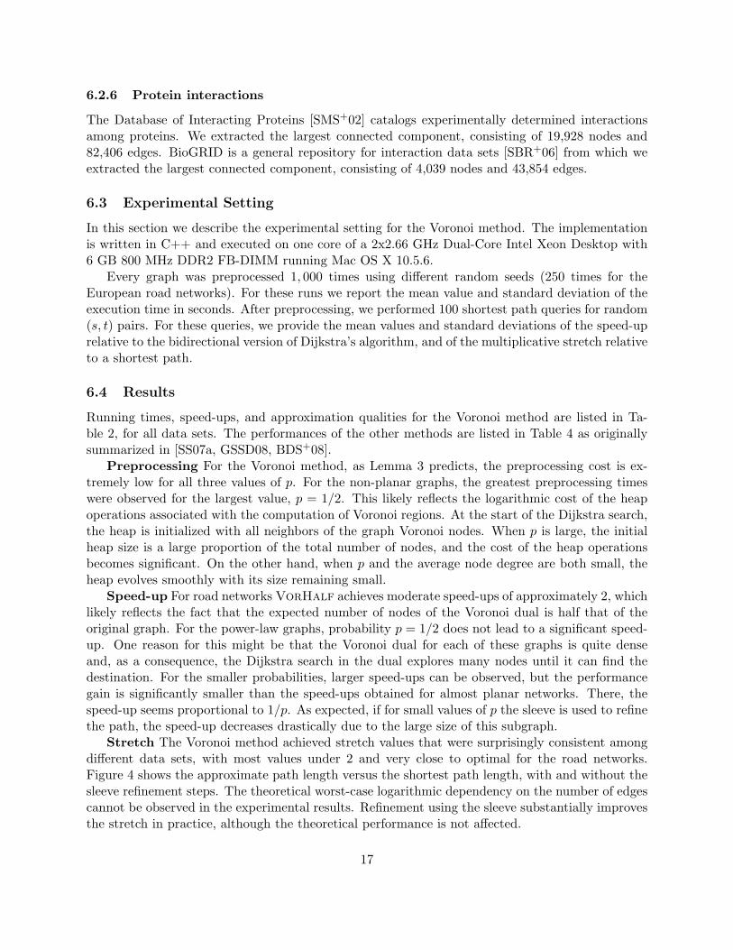
Stretch The Voronoi method achieved stretch values that were surprisingly consistent amongdifferent data sets, with most values under 2 and very close to optimal for the road networks.Figure 4 shows the approximate path length versus the shortest path length, with and without thesleeve refinement steps. The theoretical worst-case logarithmic dependency on the number of edgescannot be observed in the experimental results. Refinement using the sleeve substantially improvesthe stretch in practice, although the theoretical performance is not affected.

17

7 Conclusion

We have presented a simple and general method based on Voronoi duals to efficiently supportshortest path queries in undirected graphs with very low preprocessing overheads and competitivequery times, at the cost of exactness. The method was shown to be effective on a variety of graphtypes while remaining a reasonable alternative to existing exact methods specifically designed fortransportation networks. The results of our experiments also demonstrate that the approximationratio in practice is significantly better than the tight theoretical worst-case bound proved in themain theorem of this paper. The maximal distortion of paths in the graph Voronoi dual depends onthe distance between nodes in the original graph, unlike Delaunay triangulations of the Euclideanplane, which have constant distortion [DFS90, KG92].

An interesting topic for future research would be an expected-case analysis for weighted graphsfrom a variety of distributions.

It remains open as to whether the Voronoi method presented in this paper can be extendedto handle directed graphs. The nature of the Voronoi dual within a directed graph is inherentlydifferent from the dual within an undirected graph. The need for path connectivity suggests theconstruction of two Voronoi diagrams, one where reachability paths are oriented outward fromVoronoi nodes and another where reachability paths are oriented inward. As the respective Voronoiregions may not coincide [Erw00], it is not straightforward to define a single dual structure whoseshortest path lengths approximate those of the original graph.

References

[ACS99] Karen Aardal, Fabian A. Chudak, and David B. Shmoys. A 3-approximation algorithmfor the k-level uncapacitated facility location problem. Information Processing Letters,72:161–167, 1999.

[AGK+04] Vijay Arya, Naveen Garg, Rohit Khandekar, Adam Meyerson, Kamesh Munagala, andVinayaka Pandit. Local search heuristics for k-median and facility location problems.SIAM Journal on Computing, 33(3):544–562, 2004. Announced at STOC 2001.

[Aur91] Franz Aurenhammer. Voronoi diagrams - a survey of a fundamental geometric datastructure. ACM Computing Surveys, 23(3):345–405, 1991.

[BD08] Reinhard Bauer and Daniel Delling. SHARC: Fast and robust unidirectional rout-ing. In Proceedings of the 10th Workshop on Algorithm Engineering and Experiments(ALENEX’08), pages 13–26, 2008.

[BDS+08] Reinhard Bauer, Daniel Delling, Peter Sanders, Dennis Schieferdecker, DominikSchultes, and Dorothea Wagner. Combining hierarchical and goal-directed speed-uptechniques for Dijkstra’s algorithm. In Experimental Algorithms, 7th InternationalWorkshop (WEA’08), Provincetown, MA, USA, May 30-June 1, 2008, Proceedings,pages 303–318, 2008.

[BFM+07] Holger Bast, Stefan Funke, Domagoj Matijevic, Peter Sanders, and Dominik Schultes.In transit to constant time shortest-path queries in road networks. In Proceedings ofthe Workshop on Algorithm Engineering and Experiments (ALENEX’07), New Orleans,Louisiana, USA, January 6, 2007, 2007.

18

[BGSU08] Surender Baswana, Akshay Gaur, Sandeep Sen, and Jayant Upadhyay. Distance oraclesfor unweighted graphs: Breaking the quadratic barrier with constant additive error. InAutomata, Languages and Programming, 35th International Colloquium, ICALP 2008,Reykjavik, Iceland, July 7-11, 2008, Proceedings, Part I: Tack A: Algorithms, Automata,Complexity, and Games, pages 609–621, 2008.

[BK06] Surender Baswana and Telikepalli Kavitha. Faster algorithms for approximate distanceoracles and all-pairs small stretch paths. In 47th Annual IEEE Symposium on Foun-dations of Computer Science (FOCS 2006), 21-24 October 2006, Berkeley, California,USA, pages 591–602, 2006.

[Cha07] Timothy M. Chan. More algorithms for all-pairs shortest paths in weighted graphs. InProceedings of the 39th Annual ACM Symposium on Theory of Computing (STOC’07),pages 590–598, 2007.

[Coo03] Cooperative Association for Internet Data Analysis. Router-level topology measure-ments. Online at http://www.caida.org/tools/measurement/skitter/router topology/,file: itdk0304 rlinks undirected.gz, 2003.

[CP07] Timothy M. Chan and Mihai Patrascu. Voronoi diagrams in n · 2O(√

lg lgn) time. InProceedings of the 39th Annual ACM Symposium on Theory of Computing, San Diego,California, USA, June 11-13, 2007, pages 31–39, 2007.

[DFS90] David P. Dobkin, Steven J. Friedman, and Kenneth J. Supowit. Delaunay graphs arealmost as good as complete graphs. Discrete & Computational Geometry, 5:399–407,1990.

[Dij59] Edsger Wybe Dijkstra. A note on two problems in connexion with graphs. NumerischeMathematik, 1:269–271, 1959.

[Dir50] Gustav Lejeune Dirichlet. Uber die Reduktion der positiven quadratischen Formen mitdrei unbestimmten ganzen Zahlen. Journal fur die Reine und Angewandte Mathematik,40:209–227, 1850.

[Dor67] Jim E. Doran. An approach to automatic problem-solving. Machine Intelligence, 1:105–124, 1967.

[DSSW06] Daniel Delling, Peter Sanders, Dominik Schultes, and Dorothea Wagner. Highway hi-erarchies star. In 9th DIMACS Implementation Challenge, 2006.

[DW07] Daniel Delling and Dorothea Wagner. Landmark-based routing in dynamic graphs. InExperimental Algorithms, 6th International Workshop (WEA’07), Rome, Italy, June6-8, 2007, Proceedings, pages 52–65, 2007.

[EG08] David Eppstein and Michael T. Goodrich. Studying (non-planar) road networks throughan algorithmic lens. In 16th ACM SIGSPATIAL International Symposium on Advancesin Geographic Information Systems, ACM-GIS 2008, November 5-7, 2008, Irvine, Cal-ifornia, USA, Proceedings, page 16, 2008.

19

[EMK97] Paul Embrechts, Thomas Mikosch, and Claudia Kluppelberg. Modelling extremalevents: for insurance and finance. Springer-Verlag, London, UK, 1997.

[EP04] Michael Elkin and David Peleg. (1 + ε, β)-spanner constructions for general graphs.SIAM Journal on Computing, 33(3):608–631, 2004. Announced at STOC 2001.

[Erw00] Martin Erwig. The graph Voronoi diagram with applications. Networks, 36(3):156–163,2000.

[FT87] Michael L. Fredman and Robert Endre Tarjan. Fibonacci heaps and their uses inimproved network optimization algorithms. Journal of the ACM, 34(3):596–615, 1987.Announced at FOCS 1984.

[FW93] Michael L. Fredman and Dan E. Willard. Surpassing the information theoretic boundwith fusion trees. Journal of Computer and System Sciences, 47(3):424–436, 1993.

[GH05] Andrew V. Goldberg and Chris Harrelson. Computing the shortest path: A* searchmeets graph theory. In Proceedings of the Sixteenth Annual ACM-SIAM Symposiumon Discrete Algorithms (SODA’05), Vancouver, British Columbia, Canada, January23-25, 2005, pages 156–165, 2005.

[GKP05] Naveen Garg, Rohit Khandekar, and Vinayaka Pandit. Improved approximation for uni-versal facility location. In Proceedings of the Sixteenth Annual ACM-SIAM Symposiumon Discrete Algorithms, (SODA’05), Vancouver, British Columbia, Canada, January23-25, 2005, pages 959–960, 2005.

[GSDF03] Lise Getoor, Ted E. Senator, Pedro Domingos, and Christos Faloutsos, editors. SIGKDDProceedings, 2003.

[GSSD08] Robert Geisberger, Peter Sanders, Dominik Schultes, and Daniel Delling. Contractionhierarchies: Faster and simpler hierarchical routing in road networks. In ExperimentalAlgorithms, 7th International Workshop (WEA’08), Provincetown, MA, USA, May 30-June 1, 2008, Proceedings, pages 319–333, 2008.

[GW05] Andrew V. Goldberg and Renato Fonseca F. Werneck. Computing point-to-point short-est paths from external memory. In Proceedings of the Seventh Workshop on AlgorithmEngineering and Experiments (ALENEX’05), pages 26–40, 2005.

[HKRS97] Monika Rauch Henzinger, Philip N. Klein, Satish Rao, and Sairam Subramanian. Fastershortest-path algorithms for planar graphs. Journal of Computer and System Sciences,55(1):3–23, 1997. Announced at STOC 1994.

[KG92] J. Mark Keil and Carl A. Gutwin. Classes of graphs which approximate the completeEuclidean graph. Discrete & Computational Geometry, 7:13–28, 1992.

[Lau04] Ulrich Lauther. An extremely fast, exact algorithm for finding shortest paths in staticnetworks with geographical background. In Geoinformation und Mobilitat – von derForschung zur praktischen Anwendung, volume 22, pages 219–230, 2004.

20

[Ley02] Michael Ley. The DBLP computer science bibliography: Evolution, research issues,perspectives. In String Processing and Information Retrieval, 9th International Sympo-sium (SPIRE’02), Lisbon, Portugal, September 11-13, 2002, Proceedings, pages 1–10,2002.

[Meh88] Kurt Mehlhorn. A faster approximation algorithm for the Steiner problem in graphs.Information Processing Letters, 27(3):125–128, 1988.

[Mit03] Michael Mitzenmacher. A brief history of generative models for power law and lognormaldistributions. Internet Mathematics, 1(2), 2003.

[Ram96] Rajeev Raman. Priority queues: Small, monotone and trans-dichotomous. In Algorithms- ESA ’96, Fourth Annual European Symposium, Barcelona, Spain, September 25-27,1996, Proceedings, pages 121–137, 1996.

[Ram97] Rajeev Raman. Recent results on the single-source shortest paths problem. SIGACTNews, 28:81–87, 1997.

[SBR+06] Chris Stark, Bobby-Joe Breitkreutz, Teresa Reguly, Lorrie Boucher, Ashton Breitkreutz,and Mike Tyers. Biogrid: a general repository for interaction datasets. Nucleic AcidsResearch, 34(1):535–539, 2006.

[Sha75] Michael Ian Shamos. Geometric complexity. In Conference Record of Seventh AnnualACM Symposium on Theory of Computation (STOC’75), 5-7 May 1975, Albuquerque,New Mexico, USA, pages 224–233, 1975.

[SMS+02] Lukasz Salwinski, Christopher S. Miller, Adam J. Smith, Frank K. Pettit, James U.Bowie, and David Eisenberg. DIP, the database of interacting proteins: a researchtool for studying cellular networks of protein interactions. Nucleic Acids Research,30(1):303–305, 2002.

[SR90] Wojciech Szpankowski and Vernon Rego. Yet another application of a binomial recur-rence. Order statistics. Computing, 43(4):401–410, 1990.

[SS06] Peter Sanders and Dominik Schultes. Engineering highway hierarchies. In Algorithms- ESA 2006, 14th Annual European Symposium, Zurich, Switzerland, September 11-13,2006, Proceedings, pages 804–816, 2006.

[SS07a] Peter Sanders and Dominik Schultes. Engineering fast route planning algorithms. InExperimental Algorithms, 6th International Workshop (WEA’07), Rome, Italy, June6-8, 2007, Proceedings, pages 23–36, 2007.

[SS07b] Dominik Schultes and Peter Sanders. Dynamic highway-node routing. In Experimen-tal Algorithms, 6th International Workshop (WEA’07), Rome, Italy, June 6-8, 2007,Proceedings, pages 66–79, 2007.

[Svi08] Zoya Svitkina. Lower-bounded facility location. In Proceedings of the Nineteenth AnnualACM-SIAM Symposium on Discrete Algorithms (SODA’08), San Francisco, California,USA, January 20-22, 2008, pages 1154–1163, 2008.

21

[Tho99] Mikkel Thorup. Undirected single-source shortest paths with positive integer weightsin linear time. Journal of the ACM, 46(3):362–394, 1999. Announced at FOCS 1997.

[Tho00a] Mikkel Thorup. Floats, integers, and single source shortest paths. Journal of Algorithms,35(2):189–201, 2000. Announced at STACS 1998.

[Tho00b] Mikkel Thorup. On RAM priority queues. SIAM Journal of Computing, 30(1):86–109,2000. Announced at SODA 1996.

[Tho04a] Mikkel Thorup. Compact oracles for reachability and approximate distances in planardigraphs. Journal of the ACM, 51(6):993–1024, 2004. Announced at FOCS 2001.

[Tho04b] Mikkel Thorup. Integer priority queues with decrease key in constant time and the singlesource shortest paths problem. Journal of Computer and System Sciences, 69(3):330–353, 2004. Announced at STOC 2003.

[Tho07] Mikkel Thorup. Equivalence between priority queues and sorting. Journal of the ACM,54(6), 2007. Announced at FOCS 2002.

[TZ05] Mikkel Thorup and Uri Zwick. Approximate distance oracles. Journal of the ACM,52(1):1–24, 2005. Announced at STOC 2001.

[Vor07] Georgy Voronoi. Nouvelles applications des parametres continus a la theorie des formesquadratiques. Journal fur die Reine und Angewandte Mathematik, 133:97–178, 1907.

[Wil64] J. W. J. Williams. Algorithm 232: Heapsort. Communications of the ACM, 7:347–348,1964.

22

method preprocessing [s] without sleeve with sleevespeed-up stretch speed-up stretch

PTV European road network, driving time, 18,010,173 nodes, 42,560,279 edges

VorHalf 31.7686±4.4436 2.6061± 0.0734 1.0394±0.0131 2.5878± 0.0750 1.0111±0.0062VorRoot 40.5296±3.6423 3,518.0645± 725.2776 1.6613±0.2078 4.9991± 4.9017 1.1291±0.0783VorCubeRt 31.3372±2.8181 39,918.4988±14,207.5395 1.5544±0.4292 1.5863± 1.1123 1.0405±0.0597

PTV European road network, geographical distance, 18,010,173 nodes, 42,560,279 edges

VorHalf 29.8365±4.3576 2.6266± 0.0558 1.0307±0.0095 2.5800± 0.0627 1.0139±0.0057VorRoot 34.2785±3.0609 3,672.4070± 511.1418 1.1821±0.0960 5.9212± 7.9921 1.0390±0.0249VorCubeRt 22.5531±2.0284 42,266.6442±13,530.5983 1.2882±0.5384 1.6383± 1.4232 1.0141±0.0291

Public transportation, long distance railway, 1,586,862 nodes, 2,402,352 edges

VorHalf 2.0499±0.1998 1.9511± 0.1231 1.0180±0.0227 1.8972± 0.1367 1.0080±0.0143VorRoot 1.9086±0.0946 363.8390± 153.4644 1.3813±0.2848 2.8527± 3.3113 1.0829±0.0971VorCubeRt 1.7633±0.0860 2,116.0373± 1,251.1773 1.5167±0.6610 1.2599± 0.5990 1.0247±0.0658

Public transportation, RMV, 2,278,066 nodes, 3,417,084 edges


Public transportation, VBB, 2,600,818 nodes, 3,901,212 edges


DBLP co-authorship, 511,163 nodes, 1,871,070 edges

VorHalf 0.9145±0.0431 1.3576± 1.4690 1.2093±0.1805 1.3447± 1.4364 1.1419±0.1468VorRoot 0.8376±0.0430 37.7082± 53.2992 1.9323±0.3591 11.4432±14.8387 1.3954±0.2850VorCubeRt 0.6041±0.0312 143.8757± 208.7946 2.0033±0.3630 9.9616±12.5412 1.2881±0.2406

CAIDA router topology, 190,914 nodes, 607,610 edges

VorHalf 0.3050±0.0154 1.3164± 1.1720 1.1810±0.1703 1.2972± 1.1074 1.1283±0.1359VorRoot 0.1793±0.0092 42.4832± 54.6527 1.7845±0.3533 7.8865± 8.8062 1.2345±0.2175VorCubeRt 0.1562±0.0081 135.5521± 188.9479 1.8314±0.3755 6.0451± 7.1000 1.1621±0.1837

High energy physics citations, 27,400 nodes, 352,542 edges


Database of Interacting Proteins, 19,928 nodes, 82,406 edges


BioGRID, 4,039 nodes, 43,854 edges


Table 2: Experimental results for the Voronoi method.

23

Figure 4: Approximate path length versus actual shortest path length for VorRoot on the Euro-pean road network, distance metric. Top: using sleeve. Bottom: with sleeve steps omitted. Thetheoretical worst-case logarithmic dependency on the number of edges cannot be observed in theexperimental results. Refinement using the sleeve substantially improves the stretch in practice,although the theoretical performance is not affected.

24

PTV European road network, driving timeprep. [s] speed-up

CHHNREDS1235 [GSSD08] 602 ≈8,505A* [GH05] 780 28HH [SS06] 780 4,002HH+dist [SS06] 900 8,320HH+dist+A* [DSSW06] 1,320 11,496HNR [SS07b] 1,440 4,079CHHNREVSQWL [GSSD08] 1,914 ≈10,874TNR-eco [BFM+07] 2,760 471,881TNR-gen [BFM+07] 9,840 1,129,143

Table 3: Road networks: This table is excerpted from Sanders and Schultes [SS07a, Table 1]except for CHHNR values, which are from [GSSD08, Table 1]. Preprocessing times are convertedfrom minutes to seconds to ease comparison with our method. Machines used (except for A*): 2.0or 2.6 GHz processor, 8 or 16 GB RAM, C++ implementation.

long distance rail RMV VBB|V | 1,192,736 2,277,812 2,599,953|E| 1,789,088 3,416,552 3,899,807

prep. [s] speed-up prep. [s] speed-up prep. [s] speed-upCALT-a64 [BDS+08] 87 291.84 191 267.11 123 459.30CALT-m16 [BDS+08] 158 182.71 377 159.62 174 281.23ALT-m16 [DW07] 291 20.30 556 18.91 604 23.04CHHNR [GSSD08] 286 1,620.62 2,584 2,077.69 1,636 3,124.59CHASE [BDS+08] 536 2,660.93 2,863 4,649.26 2,008 10,398.64SHARC [BD08] 12,540 81.04 36,120 118.10

Table 4: Public transportation networks: This table is excerpted from Bauer et al. [BDS+08,p. 13]. SHARC is evaluated in [BD08, p. 10]. The speed-up is computed according to the number ofsettled nodes. Machines used: 2.0 or 2.6 GHz processor, 8 or 16 GB RAM, C++ implementation.

25

approximate shortest path queries using voronoi …) 13:)))))

Documents