Approximate CVPp in Time 20.802 n

Friedrich EisenbrandEcole Polytechnique Fédérale de Lausanne, Switzerlandfriedrich.eisenbrand@epfl.ch

Moritz VenzinEcole Polytechnique Fédérale de Lausanne, Switzerlandmoritz.venzin@epfl.ch

AbstractWe show that a constant factor approximation of the shortest and closest lattice vector problemw.r.t. any `p-norm can be computed in time 2(0.802+ε) n. This matches the currently fastest constantfactor approximation algorithm for the shortest vector problem w.r.t. `2. To obtain our result, wecombine the latter algorithm w.r.t. `2 with geometric insights related to coverings.

2012 ACM Subject Classification Theory of computation → Approximation algorithms analysis;Theory of computation → Randomness, geometry and discrete structures

Keywords and phrases Shortest and closest vector problem, approximation algorithm, sieving,covering convex bodies

Digital Object Identifier 10.4230/LIPIcs.ESA.2020.43

Funding The authors acknowledge support from the Swiss National Science Foundation within theproject Lattice Algorithms and Integer Programming (Nr. 200021-185030).

Acknowledgements The authors would like to thank the reviewers for their careful reviews andsuggestions. The second author would like to thank Christoph Hunkenschröder, Noah Stephens-Davidowitz and Márton Naszódi for inspiring discussions.

1 Introduction

The shortest vector problem (SVP) and the closest vector problem (CVP) are importantalgorithmic problems in the geometry of numbers. Given a rational lattice

L(B) = {Bx : x ∈ Zn}

with B ∈ Qn×n and a target vector t ∈ Qn the closest vector problem asks for lattice vectorv ∈ L(B) minimizing ‖t− v‖. The shortest vector problem asks for a nonzero lattice vectorv ∈ L(B) of minimal norm. When using the `p norms for 1 ≤ p ≤ ∞, we denote the problemsby SVPp resp. CVPp.

Much attention has been devoted to the hardness of approximating SVP and CVP. In along sequence of papers, including [42, 7, 32, 10, 18, 28, 23] it has been shown that SVP andCVP are hard to approximate to within almost polynomial factors under reasonable com-plexity assumptions. The best polynomial-time approximation algorithms have exponentialapproximation factors [29, 41, 8].

The first algorithm to solve CVP for any norm that has exponential running time in thedimension only was given by Lenstra [30]. The running time of his procedure is 2O(n2) timesa polynomial in the encoding length. In fact, Lenstra’s algorithm solves the more generalinteger programming problem. Kannan [27] improved this to nO(n) time and polynomialspace. It took almost 15 years until Ajtai, Kumar and Sivakumar presented a randomizedalgorithm for SVP2 with time and space 2O(n) and a 2O(1+1/ε)n time and space algorithmfor (1 + ε)-CVP2 [8, 9]. Here (1 + ε)-CVP2 is the problem of finding a lattice vector, whose

© Friedrich Eisenbrand and Moritz Venzin;licensed under Creative Commons License CC-BY

28th Annual European Symposium on Algorithms (ESA 2020).Editors: Fabrizio Grandoni, Grzegorz Herman, and Peter Sanders; Article No. 43; pp. 43:1–43:15

Leibniz International Proceedings in InformaticsSchloss Dagstuhl – Leibniz-Zentrum für Informatik, Dagstuhl Publishing, Germany

43:2 Approximate CVPp in Time 20.802 n

distance to the target is at most 1 + ε times the minimal distance. Blömer and Naewe [14]extended the randomized sieving algorithm of Ajtai et al. to solve SVPp and obtain a 2O(n)

time and space exact algorithm for SVPp and an O(1 + 1/ε)2n time algorithm to computea (1 + ε) approximation for CVPp. For CVP∞, one has a faster approximation algorithm.Eisenbrand et al. [20] showed how to boost any constant approximation algorithm for CVP∞to a (1 + ε)-approximation algorithm in time O(log(1 + 1/ε))n. Recently, this idea wasadapted in [36] to all `p norms, showing that (1 + ε) approximate CVPp can be solved intime O(1 + 1/ε)n/min(2,p) by boosting the deterministic CVP algorithm for general (evenasymmetric) norms with a running time of (1 + 1/ε)n that was developed by Dadush andKun [16].

The first deterministic singly-exponential time and space algorithm for exact CVP2 (andSVP2) was developed by [33]. The fastest exact algorithms for SVP2 and CVP2 run in timeand space 2n+o(n) [3, 1, 6]. Single exponential time and space algorithms for exact CVP areonly known for `2. Whether CVP and the more general integer programming problem canbe solved in time 2O(n) is a prominent mystery in algorithms.

Recently there has been exciting progress in understanding the fined grained complexityof exact and constant approximation algorithms for CVP [2, 12, 5]. Under the assumption ofthe strong exponential time hypothesis (SETH) and for p 6= 0 (mod 2), exact CVPp cannotbe solved in time 2(1−ε)d. Here d is the ambient dimension of the lattice, which is the numberof vectors in a basis of the lattice. Under the assumption of a gap-version of the strongexponential time hypothesis (gap-SETH) these lower bounds also hold for the approximateversions of CVPp. More precisely, for each ε > 0 there exists a constant γε > 1 such thatthere exits no 2(1−ε)d algorithm that computes a γε-approximation of CVPp.

Unfortunately, the currently fastest algorithms for CVPp resp. SVPp do not matchthese lower bounds, even for large approximation factors. These algorithms are based onrandomized sieving, [8, 9]. Many lattice vectors are generated that are then, during manystages, subtracted from each other to obtain shorter and shorter vectors w.r.t. `p (resp.any norm) until a short vector is found. However, the algorithm needs to start out withsufficiently many lattice vectors just to guarantee that two of them are close. This issuedirectly relates to the kissing number (w.r.t. some norm) which is the maximum number ofunit norm balls that can be arranged so that they touch another given unit norm ball. In thesetting of sieving, this is the number of vectors of length r that are needed to guarantee thatthe difference of two of them is strictly smaller than r. Among all known upper bounds onthe kissing numbers, the best (i.e. smallest) upper bound is known for `2 and equals 20.401n,[26]. For `2 the fastest such approximation algorithms require time 20.802n - the square ofthe kissing number w.r.t. `2. For `∞ the kissing number equals 3n− 1 which is also an upperbound on the kissing number for any norm. The current best constant factor approximationalgorithms for SVP∞ and CVP∞ require time 3n, their counterparts w.r.t. `p require evenmore time, see [4, 35]. This then suggests the question, originally raised by Aggarwal et al.in [2] for `∞, whether the kissing number w.r.t. `p is a natural lower bound on the runningtime of SVPp resp. CVPp.

Our results indicate otherwise. For constant approximation factors, we are able to reducethese problems w.r.t. `p to another lattice problem but w.r.t. `2. This directly improves therunning time of the algorithms for `p norms that hinge on the kissing number. Furthermore,given that the development of algorithms for `2 has been much more dynamic than forarbitrary `p norms and the difficulty of establishing hardness results for `2, there is hope tofind still faster algorithms for SVP2 that may not even rely on the kissing number w.r.t. `2.It is likely that this would then improve the situation for `p norms as well.

F. Eisenbrand and M. Venzin 43:3

Our main results are resumed in the following theorem.I Theorem. For each ε > 0, there exists a constant γε such that a γε approximate solutionto CVPp, as well as to SVPp for p ∈ [1,∞] can be found in time 2(0.802+ε)n.Our main idea is to use coverings in order to obtain a constant factor approximation to theshortest resp. closest vector w.r.t. `p by using a (approximate) shortest vector algorithmw.r.t. `2. We need to distinguish between the cases p ∈ [2,∞] and p ∈ [1, 2). For p ∈ [2,∞],we show that exponentially many short vectors w.r.t. `2 cannot all have large pairwisedistance w.r.t. `p. This follows from a bound on the number of `p norm balls scaled by someconstant that are required to cover the `2 norm ball of radius n1/2−1/p. The final procedureis then to sieve w.r.t. `2 and to pick the smallest non zero pairwise difference w.r.t. `p of the(exponentially many) generated lattice vectors. This yields a constant factor approximationto the shortest resp. closest vector w.r.t. `p, p ∈ [2,∞]. For p ∈ [1, 2), we use a more directcovering idea. There is a collection of at most 2εn balls w.r.t. `2, whose union contains the`p norm ball but whose union is contained in the `p norm ball scaled by some constant. Thisleads to a simple algorithm for `p norms (p ∈ [1, 2)) by using the approximate closest vectoralgorithm w.r.t. `2 from this paper.This paper is organized as follows. In Section 2 we present the main idea for p =∞ that alsoapplies to the case p ≥ 2. In Section 3 we first reintroduce the list-sieve method originallydue to [34] but with a slightly more general viewpoint, we resume this in Theorem 4. Wethen present in detail our approximate CVP∞ resp. SVP∞ algorithm and extend this idearesp. algorithm to `p, p ≥ 2. This is Theorem 5. Finally, in Section 4, using the coveringtechnique from Section 2 and our approximate CVP2 algorithm from Section 3.1, we showhow to solve approximate CVPp for p ∈ [1, 2). This is Theorem 8.

2 Covering balls with boxes

We now outline our main idea in the setting of an approximate SVP∞ algorithm. Let usassume that the shortest vector of L w.r.t. `∞ is s ∈ L \ {0}. We can assume that thelattice is scaled such that ‖s‖∞ = 1 holds. The euclidean norm of s is then bounded by√n. Suppose now that there is a procedure that, for some constant γ > 1 independent of n,

generates distinct lattice vectors v1, . . . ,vN ∈ L of length at most ‖vi‖2 ≤ γ√n.

γ√n

vi

vj

α/2

Figure 1 The difference vi − vj is an α-approximate shortest vector w.r.t. `∞.

How large does the number of vectors N have to be such that we can guarantee thatthere exist two indices i 6= j with

‖vi − vj‖∞ ≤ α, (1)

ESA 2020

43:4 Approximate CVPp in Time 20.802 n

where α ≥ 1 is the approximation guarantee for SVP∞ that we want to achieve? Supposethat N is larger than the minimal number of copies of the box (α/2)Bn∞ that are requiredto cover the ball

√nBn2 . Here Bnp = {x ∈ Rn : ‖x‖p ≤ 1} denotes the unit ball w.r.t. the

`p-norm. Then, by the pigeon-hole principle, two different vectors vi and vj must be inthe same box. Their difference satisfies (1) and thus is an α-approximate shortest vectorw.r.t. `∞, see Figure 1.

Thus we are interested in the translative covering number N(√nBn2 , aB

n∞), which is the

number of translated copies of the box aBn∞ that are needed to cover the `2-ball of radius√n.

In the setting above, a is the constant α/(2γ). For this procedure to be efficient, we needN(√nBn2 , aB

n∞) to be relatively small for a large enough - this is equivalent to decreasing

the number of vectors N we need to generate by worsening (increasing) the approximationguarantee α. Since 2O(n) vol(Bn∞) = vol(

√nBn2 ) and by a simple covering argument, we have

that N(√nBn2 , B

n∞) ≤ 2Cn. This gives hope that by taking a large enough (but independent

of n), we can decrease N(√nBn2 , aB

n∞) to, say, 20.401n or 2εn for ε > 0.

Covering problems like these have received considerable attention in the field of convexgeometry, see [11, 37]. These techniques rely on the classical set-cover problem and thelogarithmic integrality gap of its standard LP-relaxation, see, e.g. [43, 15]. To keep thispaper self-contained, we briefly explain how this can be applied to our setting.

If we cover the finite set (1/n)Zn ∩√nBn2 with cubes whose centers are on the grid

(1/n)Zn, then by increasing the side-length of those cubes by an additive 1/n, one obtains afull covering of

√nBn2 . Thus we can focus on the corresponding set-covering problem with

ground set U = (1/n)Zn ∩√nBn2 and sets

St = U ∩ aBn∞ + t, t ∈ (1/n)Zn,

ignoring empty sets. An element of the ground set is contained in exactly |(1/n)Zn ∩ aBn∞|many sets. Therefore, by assigning each element of the ground set the fractional value1/|(1/n)Zn ∩ aBn∞|, one obtains a feasible fractional covering. The weight of this fractionalcovering is

T

|(1/n)Zn ∩ aBn∞|

where T is the number of sets. Clearly, if a cube intersects√nBn2 , then its center is contained

in the Minkowski sum√nBn2 + aBn∞ and thus the weight of the fractional covering is

|(√nBn2 + aBn∞) ∩ 1

nZn|

| 1nZn ∩ aBn∞|= O

(vol(√nBn2 + aBn∞)

vol(aBn∞)

)Since the size of the ground-set is bounded by nO(n) and since the integrality gap of theset-cover LP is at most the logarithm of this size, one obtains

N(√nBn2 , aB

n∞) ≤ poly(n) vol(

√nBn2 + aBn∞)

vol(aBn∞) (2)

By Steiner’s formula, see [22, 40, 24], the volume of K + tBn2 is a polynomial in t, withcoefficients Vj(K) only depending on the convex body K:

vol(K + tBn2 ) =n∑j=0

Vj(K) vol(Bn−j2 )tn−j

For K = aBn∞, Vj(K) = (2a)j(nj

). Setting t =

√n, the resulting expression has been

evaluated in [25, Theorem 7.1].

F. Eisenbrand and M. Venzin 43:5

I Theorem 1 ([25]). Denote by H the binary entropy function and let φ ∈ (0, 1) the uniquesolution to

1− φ2

φ3 = 2a2

π(3)

Then

vol(aBn∞ +√nBn2 ) = O(2n[H(φ)+(1−φ) log(2a)+φ

2 log( 2πeφ )])

Using this bound in inequality (2) and simplifying, we find

N(√nBn2 , aB

n∞) ≤ poly(n) 2n[H(φ)+φ

2 log( 2πeφ )]

Both H(φ) and φ2 log( 2πe

φ ) decrease to 0 as φ decreases to 0. Since φ, the unique solution to(3), satisfies φ ≤ 3

√(π/2)a− 2

3 , we obtain the following bound.

I Lemma 2. For each ε > 0, there exists aε ∈ R>0 independent of n, such that

N(√nBn2 , aεB

n∞) ≤ 2εn.

Going back to the idea for an approximate SVP∞ algorithm, we will use Lemma 2 withε = 0.401. If we generate 20.401n distinct lattice vectors of euclidean length at most γ

√n,

then there must exist a pair of lattice vectors with pairwise distance w.r.t. `∞ shorter than2γa0.401. We find it by trying out all possible pairwise combinations, this takes time 20.802n.

The main idea for approximate SVPp is similar. Set s the shortest vector in L w.r.t. `pand scale the lattice so that ‖s‖p = 1. The euclidean norm of s is bounded by n1/2−1/p.Again, we can consider the question of how many different lattice vectors there have tobe within a ball of radius γn1/2−1/p so that we can guarantee that there exist two latticevectors with constant pairwise distance w.r.t. `p. This leads us to consider the translativecovering number N(n1/2−1/pBn2 , aB

np ). Since n−1/pBn∞ ⊆ Bnp , the following is immediate

from Lemma 2.

I Lemma 3. For each ε > 0, there exists aε ∈ R>0 independent of n, such that

N(n1/2−1/pBn2 , aεBnp ) ≤ 2εn.

3 Approximate CVPp for p ≥ 2

We now describe our main contribution. As we mentioned already, SVP2 can be approximatedup to a constant factor in time 2(0.802+ε)n for each ε > 0. This follows from a careful analysisof the list sieve algorithm of Micciancio and Voulgaris [34], see [31, 38]. The running time andspace of this algorithm is directly related to the kissing number of the `2-norm. The runningtime is the square of the best known upper bound by Kabatiansky and Levenshtein [26].

The main insight of our paper is that the current list-sieve variants can be used toapproximate SVPp and CVPp by testing all pairwise differences of the generated latticevectors.

3.1 List sieveWe begin by describing the list-sieve method [34] to a level of detail that is necessary tounderstand our main result. Our exposition follows closely the one given in [38]. Let L(B)be a given lattice and s ∈ L be an unknown lattice vector. This unknown lattice vector s istypically the shortest, respectively closest vector in L(B).

ESA 2020

43:6 Approximate CVPp in Time 20.802 n

The list-sieve algorithm has two stages. The input to the first stage of the algorithm isan LLL-reduced lattice basis B of L(B), a constant ε > 0 and a guess µ on the length of sthat satisfies

‖s‖2 ≤ µ ≤ (1 + 1/n)‖s‖2. (4)

The first stage then constructs a list of lattice vectors L ⊆ L(B) that is random. This list oflattice vectors is then passed on to the second stage of the algorithm.

The second stage of the algorithm proceeds by sampling points y1, . . . ,yN uniformly andindependently at random from the ball

(ξε · µ)Bn2 ,

where ξε is an explicit constant depending on ε only. It then transforms these points via adeterministic algorithm ListRedL into lattice points

ListRedL(y1), . . . , ListRedL(yN ) ∈ L(B).

The deterministic algorithm ListRedL uses the list L ⊆ L(B) from the first stage.

−s 0

IS

ξε · µBn2

−s + ξε · µBn2

Figure 2 The lens Is.

As we mentioned above, the list L ⊆ L(B) that is used by the deterministic algorithmListRedL is random. We will show the following theorem in the next section. The noveltycompared to the literature is the reasoning about pairwise differences lying in centrallysymmetric sets. In this theorem, ε > 0 is an arbitrary constant, ξε as well as cε are explicitconstants and K is some centrally symmetric set. Furthermore, we assume that µ satisfies (4).

The theorem reasons about an area Is that is often referred as the lens, see Figure 2.The lens was introduced by Regev as a conceptual modification to facilitate the proof of theoriginal AKS algorithm [39].

Is = (ξε · µ)Bn2 ∩ (−s + (ξε · µ)Bn2 ) (5)

I Theorem 4. With probability at least 1/2, the list L that was generated in the first stagesatisfies the following. If y1, · · · ,yN are chosen independently and uniformly at randomwithin Bn2 (0, ξεµ) theni) The probability of the event that two different samples yi,yj satisfy

yi,yj ∈ Is and ListRedL(yi)− ListRedL(yj) ∈ K

is at most twice the probability of the event that two different samples yi,yj satisfy

ListRedL(yi)− ListRedL(yj) ∈ K + s

F. Eisenbrand and M. Venzin 43:7

ii) For each sample yi the probability of the event

‖ListRedL(yi)‖2 ≤ cε ‖s‖2 and yi ∈ Is

is at least 2−εn.The complete procedure, i.e. the construction of the list L in stage one and applyingListRedL to the N samples y1, . . . ,yn in stage two takes time N2(0.401+ε)n + 2(0.802+ε)n

and space N + 2(0.401+ε)n.The proof of Theorem 4 follows verbatim from Pujol and Stehlé [38], see also [31]. In [38],

s is a shortest vector w.r.t. `2. But this fact is never used in the proof and in the analysis.Part ii) follows from Lemma 5 and Lemma 6 in [38]. Their probability of a sample being inthe lens Is ⊆ ξ ‖s‖2 B

n2 depends only on ξ (corresponding to our ξε). By choosing ξ large

enough, this happens with probability at least 2−εn. Their Lemma 6 then guarantees thatthe list L, with probability 1/2, when yi ∼ Is is sampled uniformly, returns a lattice vectorof length at most r0 ‖s‖2 (r0 corresponds to our cε). This corresponds to part ii) in oursetting. The size of their list (denoted by NT ) is bounded above by 2(0.401+δ)n where δ > 0decreases to 0 as the ratio r0/ξ increases, this is their Lemma 4.

Finally, part i) also follows from Pujol and Stehlé [38]. It is in their proof of correctness,Lemma 7, involving the lens Is. We briefly comment on our general viewpoint. Giveny ∼ (ξ · µ)Bn2 , the algorithm computes the linear combination w.r.t. to the lattice basisb1, . . . ,bn

y =n∑i=1

λibi

and then the remainder

y (mod L) =n∑i=1bλicbi.

The important observation is that this remainder is the same for all vectors y + v, v ∈ L.Next, it keeps reducing (minus) the remainder w.r.t. the list, as long as the length decreases.This results in a vector of the form

−y (mod L)− v1 − · · · − vk, for some vi ∈ L.

The output ListRedL(y) is then

−y (mod L)− v1 − · · · − vk + y ∈ L.

The algorithm bases its decisions on y (mod L) and not on y directly. This is why onecan imagine that, after y (mod L) has been created, one applies a bijection τ of the ballτ(·) : ξµBn2 → ξµBn2 on y with probability 1/2. For y ∈ Is one has τ(y) = y + s. We referto [38] for the definition of τ . Since τ is a bijection and preserves the measure, the resultof applying τ(y) with probability 1/2 is distributed uniformly. This means that for y ∈ Isthis modified but equivalent procedure outputs ListRedL(y) or ListRedL(y) + s, both withprobability 1/2. If ListRedL(yi)− ListRedL(yj) ∈ K, we toss a coin for i and j each. Withprobability 1/2, their difference is in ±K + s.

3.2 Approximation to CVPp and SVPp for p ∈ [2,∞]We now combine Theorem 4 with the covering ideas presented in Section 2.

ESA 2020

43:8 Approximate CVPp in Time 20.802 n

I Theorem 5. For p ≥ 2, there is a randomized algorithm that computes with constantprobability a constant factor (depending on ε) approximation to CVPp and SVPp respectively.The algorithm runs in time 2(0.802+ε)n and it requires space 2(0.401+ε)n.

In short, the algorithm is the standard list-sieve algorithm with a slight twist: Check allpairwise differences.We first present in detail the case p =∞. Even though there is an approximation preservingreduction from SVP to CVP, [21], we present separately the case SVP and CVP to highlightthe ideas from Section 2 and Theorem 4. The case p ≥ 2 then follows from this, we brieflycomment on it.

Proof for p =∞. We assume that the list L that was computed in the first stage satisfiesthe properties described in Theorem 4. Recall that this is the case with probability atleast 1/2.We first consider SVP∞. By Lemma 2, there is a > 0 such that N(

√nBn2 , aB

n∞) ≤ 20.401n.

Let s be a shortest vector w.r.t. `∞ and let µ > 0 such that ‖s‖2 ≤ µ < (1 + 1n ) ‖s‖2 as

above. Since ‖s‖2 ≤√n ‖s‖∞ we have N(cε ‖s‖2 B

n2 , cεa ‖s‖∞Bn∞) ≤ 20.401n. This means

that, if d20.401ne+ 1 lattice vectors are contained in the ball cε‖s‖2Bn2 at least two of them

have `∞-distance bounded by 2cεa which is a constant.Set N = 2 · d2(ε+0.401)n+ 1e and {y1, . . . ,yN}

iid∼ Bn2 (0, ξεµ) uniformly and independentlyat random. By Theorem 4 ii) and by the Chebychev inequality, see [38], the following eventhas probability at least 1/2.

(Event A): There is a subset S ⊆ {1, . . . , N} with |S| = d20.401ne+ 1 such that foreach i ∈ S

yi ∈ Is and ‖ ListRedL(yi)‖2 ≤ cε‖s‖2. (6)

This event is the disjoint union of the event A ∩B and A ∩B, where B denotes the eventwhere the vectors ListRedL(yi), yi ∈ Is are all distinct. Thus

Pr(A) = Pr(A ∩B) + Pr(A ∩B).

The probability of at least one of the events A ∩B and A ∩B is bounded below by 1/4. Inthe event A ∩B, there exists i 6= j such that

‖ ListRedL(vi)− ListRedL(vj)‖∞ ≤ 2cεa.

By Theorem 4 i) with K = {0} one has

Pr(A ∩B) ≤ 2 Pr (∃i 6= j : ListRedL(vi)− ListRedL(vj) = s) .

Therefore, with constant probability, there exist i, j ∈ {1, . . . , N} with

0 < ‖ ListRedL(yi)− ListRedL(yj)‖∞ ≤ 2cεa.

We try out all the pairs of N elements, which amounts to N2 = 2(0.802+ε′)n additional time.We next describe how list-sieve yields a constant approximation for CVP∞. Let w ∈ L(B)

be the closest lattice vector w.r.t. `∞ to t ∈ Rn and let µ > 0 such that ‖t−w‖2 ≤ µ <

(1 + 1n ) ‖t−w‖2. We use Kannan’s embedding technique [27] and define a new lattice L′

with basis

B =(B t0 1

nµ

)∈ Q(n+1)×(n+1),

F. Eisenbrand and M. Venzin 43:9

Finding the closest vector to t w.r.t. `∞ in L(B) amounts to finding the shortest vectorw.r.t. `∞ in L′(B) ∩ {x ∈ Rn+1 : xn+1 = 1

nµ}. The vector s = (t−w, 1nµ) is such a vector

and its euclidean length is smaller than (1 + 1n )µ. Let a > 0 be such that

N(√nBn2 , aB

n∞) ≤ 20.401n.

This means that there is a covering of the n-dimensional ball (cε‖s‖2)Bn+12 ∩ {x ∈ Rn+1 :

xn+1 = 0} by 20.401n translated copies of K, where

K = (cε · a(1 + 1/n)‖s‖∞)Bn+1∞ ∩ {x ∈ Rn+1 : xn+1 = 0}. (7)

(The factor (1 + 1/n) is a reminiscent of the embedding trick, s is n + 1 dimensional.)Similarly, we may cover (cε‖s‖2)Bn+1

2 ∩ {x ∈ Rn+1 : xn+1 = k · µn} for all k ∈ Z (such thatthe intersection is not empty) by translates of K. There are only 2cε(n+ 1) + 1 such layersto consider and so (2cε(n+ 1) + 1)20.401n translates of K suffice. The last component of alattice vector of L′ is of the form k · µn and it follows that these translates of K cover alllattice vectors of euclidean norm smaller than cε ‖s‖2, see Figure 3.

cǫ‖s‖2

xn+1 = µ/n

xn+1 = 2µ/nvivj

s

xn+1 = 0

K

Figure 3 Covering the lattice points with translates of K..

Set N = d(2cε(n+1)+2)2(ε+0.401)ne and sample again {y1, . . . ,yN}iid∼ Bn2 (0, ξεµ) uniformly

and independently at random. By Theorem 4 ii) and by the Chebychev inequality, see [38],the following event has a probability at least 1/2.

(Event A′): There is a subset S ⊆ {1, . . . , N} with |S| = (2cε(n+ 1) + 1)20.401n + 1such that for each i ∈ S

yi ∈ Is and ‖ ListRedL(yi)‖2 ≤ cε‖s‖2. (8)

In this case, there exists a translate of K that holds at least two vectors ListRedL(yi) andListRedL(yj) for different samples yi and yj , see Figure 3 with vi,vj ∈ L′ instead. Thus,with probability at least 1/2, there are i, j ∈ [N ] with yi,yj ∈ Is such that

ListRedL(yi)− ListRedL(yj) ∈ 2K

Theorem 4 i) implies that, with probability at least 1/4, there exist different samples yi andyj such that

ListRedL(yi)− ListRedL(yj) ∈ 2K + s

ESA 2020

43:10 Approximate CVPp in Time 20.802 n

In this case, the first n coordinates of ListRedL(yi)− ListRedL(yj) can be written of theform t− v for v ∈ L and the first n coordinates on the right hand side are of the of the form(t −w) + z, where z ∈ L′ and ‖z‖∞ ≤ 2cε(1 + 1/n)a ‖s‖∞ = 2cε(1 + 1/n)a ‖t−w‖∞. Inparticular, the lattice vector v ∈ L is a 2acε(1 + 1/n) + 1 approximation to the closest vectorto t. Since we need to try out all pairs of the N elements, this takes time N2 = 2(0.802+ε′)n

and space N . J

I Remark 6. For clarity we have not optimized the approximation factor. There are variousways to do so. We remark that for SVP∞ we actually get a smaller approximation factorthan the one that we describe. Let a be such that N(

√nBn2 , aB

n∞) ≤ 20.802n, the algorithm

described above yields a 2cεa approximation instead of a 2cεa approximation to the shortestvector. This follows by applying the birthday paradox in the way that it was used by Pujoland Stehlé [38]. The same argument also applies to CVP∞. Finally, we remark that in thecase of SVP we have not really used property i) of Theorem 4. We only use this property toensure that the generated vectors are different. It is plausible that this can be done moreefficiently or with a better approximation factor.

Proof continued, p ≥ 2. For SVPp, p ≥ 2, we define s to be shortest vector w.r.t. `p instead.Since ‖s‖2 ≤ n1/2−1/p ‖s‖p, we simply use Lemma 3 instead of Lemma 2 to conclude thatthere is some a > 0 such that if we have a set of 20.401n different lattice vectors of (euclidean)length smaller than cε ‖s‖2, then two of them must have pairwise distance smaller than 2cεaw.r.t. `p.For CVPp, we define w to be the closest lattice vector to t w.r.t. `p. Both s and L′ aredefined analogously. We will need to replace the convex body K in (7) by

K = (cε · a(1 + 1/n)‖s‖p)Bn+1p ∩ {x ∈ Rn+1 : xn+1 = 0}.

The respective algorithms for SVPp and CVPp and the proof of correctness now follow fromthe case p =∞. In particular, we can use the same parameters cε and a.

For the important case p = 2 we note that we can chose a = 1. This yields a approximationto the closest vector with the approximation guarantee cε matching that of the fastestapproximate shortest vector problem w.r.t. `2, see [31]. J

4 Approximate CVPp for p ∈ [1, 2)

In the previous section, we have extended the approximate SVP2 solver to yield constantfactor approximations to SVPp and CVPp for p ∈ [2,∞] in time 2(0.802+ε)n. From simplevolumetric considerations, the technique from the previous section cannot be adapted tosolve SVPp and CVPp for p ∈ [1, 2) (in single exponential time). Instead, we can use a simplecovering technique similar to the one considered by Eisenbrand et al. in [20]. We first showthat for any constant ε > 0, there is a constant aε > 0, so that the crosspolytope Bn1 can becovered by 2εn balls (w.r.t. `2) with radius (aε/

√n) and whose union is contained inside

the crosspolytope scaled by aε. A similar covering also exists for Bnp . Using the centers ofthese balls as targets, we can use the approximate CVP2 algorithm to solve approximateCVP1 resp. CVPp. This is also similar to the technique of Dadush et al. in [17] resp. [16]where they cover general norm balls with M-ellipsoids to solve SVP and CVP w.r.t. tothis norm by using the CVP2 algorithm due to [33]. Unfortunately, there is only an upperbound of 2Cn for some (large) constant C > 0 on the number of required M-ellipsoids, forour purpose we need a finer estimate. To achieve this, we rely on the set-covering idea andvolume computations as outlined in Section 2. The following analogue to Lemma 2 is shownin the appendix.

F. Eisenbrand and M. Venzin 43:11

I Lemma 7. For each ε > 0, there exists aε ∈ R>0 independent of n such that

vol(Bn1 + (aε/√n)Bn2 )

vol((aε/√n)Bn2 )

≤ 2εn.

We now sketch the covering procedure for CVP1 and SVP1. Up to scaling the lattice and aguess on the distance of the closest (resp. shortest) lattice vector v to the target t, we mayassume that 1 − 1/n ≤ ‖v− t‖1 ≤ 1 (resp. 1 − 1/n ≤ ‖v‖1 ≤ 1). We uniformly sample apoint x, [19], within t + Bn1 + (aε/

√n)Bn2 (set t = 0 for SVP1) and place a ball of radius

aε/√n around x (or x′, the closest point to x in Bn1 , see Fig. 4).

x

x′

v

Bn

1+ (c/

√

n)Bn

2

Bn

1

x+ (c/√

n)Bn

2

Figure 4 Generating a covering of Bn1 by (c/

√n)Bn

2 ..

By Lemma 7, with probability at least 2−εn, v is covered by x+(aε/√n)Bn2 . Running the

c-approximate (randomized) CVP2 algorithm with target x (provided ‖v− x‖2 ≤ (aε/√n)),

a lattice vector w ∈ x + (c · aε/√n)Bn2 ⊆ t + c · (aε + 1)Bn1 is returned. The lattice vector

w is thus a c · (aε + 1) approximation to the closest (resp. shortest) vector. In general, werun the c-approximate CVP2 algorithm O(poly(n)2εn) times with targets uniformly chosenwithin t +Bn1 + (aε/

√n)Bn2 and only output the closest of the resulting lattice vectors if it

is within c · (aε + 1)Bn1 . This ensures that, if there is lattice vector v in t +Bn1 , a constantfactor approximation to ‖t− v‖1 is found with high probability.The same covering technique can be applied to Bnp , p ∈ (1, 2). By Hölder’s inequality,

Bnp ⊆ n1−1/pBn1 and n1/2−1/pBn2 ⊆ Bnp .

The first of these inclusions implies that for any ε > 0, we can pick the same constant aε asin Lemma 7 and cover Bnp by at most 2εn translates of aεn1/2−1/pBn2 .

vol(Bnp + cn1/2−1/pBn2 )vol(cn1/2−1/pBn2 )

≤ vol(n1−1/pBn1 + cn1/2−1/pBn2 )vol(cn1/2−1/pBn2 )

= vol(Bn1 + (c/√n)Bn2 )

vol((c/√n)Bn2 )

The second inclusion implies that these translates do not overlap Bnp by more then a constantfactor. It is then straightforward to adapt the boosting procedure described for CVP1 toCVPp. Using the approximate CVP2 algorithm from the previous section then implies thefollowing algorithm.

I Theorem 8. There is a randomized algorithm that computes with constant probability aconstant (depending on ε) factor approximation to CVPp, p ∈ [1, 2). The algorithm runs intime 2(0.802+ε)n and requires space 2(0.401+ε)n.

ESA 2020

43:12 Approximate CVPp in Time 20.802 n

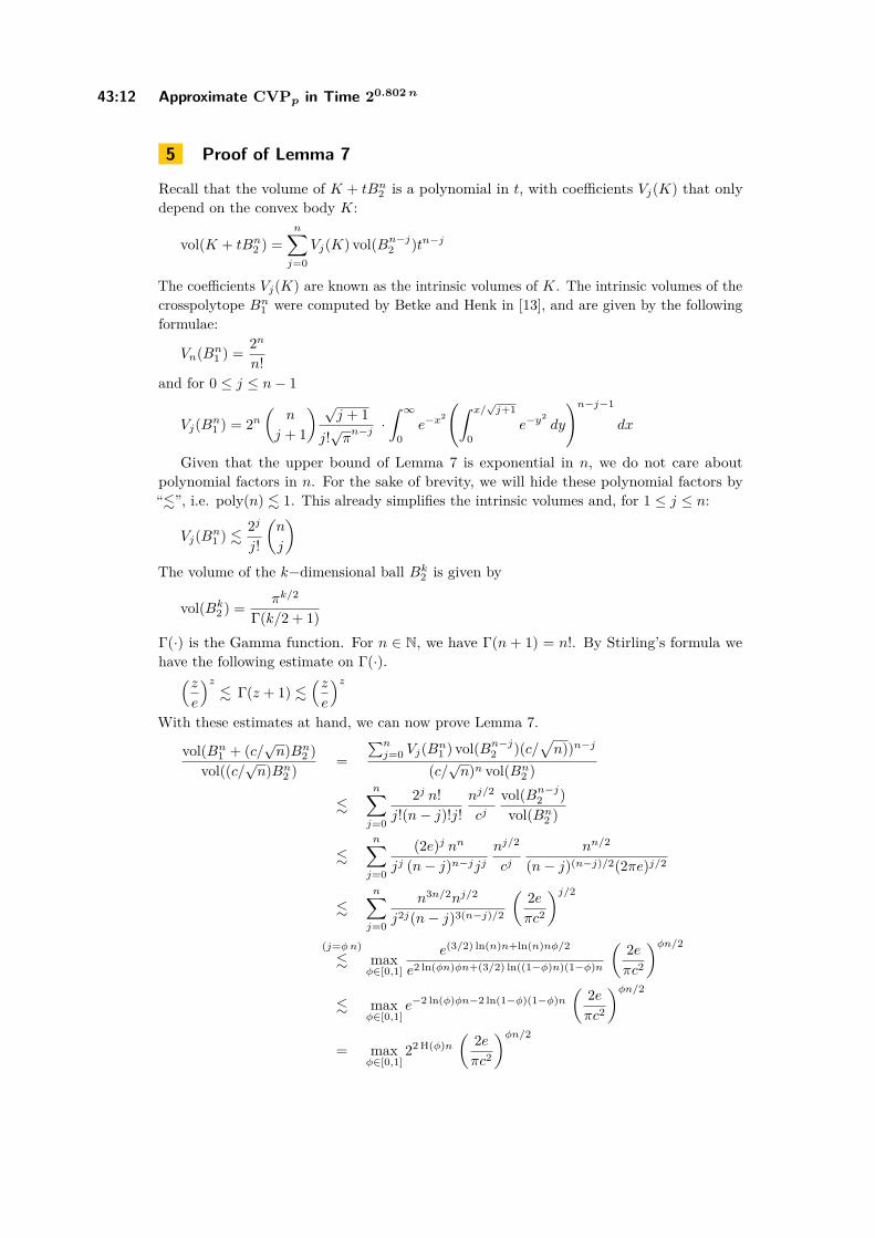
5 Proof of Lemma 7

Recall that the volume of K + tBn2 is a polynomial in t, with coefficients Vj(K) that onlydepend on the convex body K:

vol(K + tBn2 ) =n∑j=0

Vj(K) vol(Bn−j2 )tn−j

The coefficients Vj(K) are known as the intrinsic volumes of K. The intrinsic volumes of thecrosspolytope Bn1 were computed by Betke and Henk in [13], and are given by the followingformulae:

Vn(Bn1 ) = 2n

n!and for 0 ≤ j ≤ n− 1

Vj(Bn1 ) = 2n(

n

j + 1

) √j + 1

j!√πn−j ·

∫ ∞0

e−x2

(∫ x/√j+1

0e−y

2dy

)n−j−1

dx

Given that the upper bound of Lemma 7 is exponential in n, we do not care aboutpolynomial factors in n. For the sake of brevity, we will hide these polynomial factors by“.”, i.e. poly(n) . 1. This already simplifies the intrinsic volumes and, for 1 ≤ j ≤ n:

Vj(Bn1 ) . 2j

j!

(n

j

)The volume of the k−dimensional ball Bk2 is given by

vol(Bk2 ) = πk/2

Γ(k/2 + 1)Γ(·) is the Gamma function. For n ∈ N, we have Γ(n+ 1) = n!. By Stirling’s formula wehave the following estimate on Γ(·).(z

e

)z. Γ(z + 1) .

(ze

)zWith these estimates at hand, we can now prove Lemma 7.

vol(Bn1 + (c/√n)Bn2 )

vol((c/√n)Bn2 )

=∑nj=0 Vj(Bn1 ) vol(Bn−j2 )(c/

√n))n−j

(c/√n)n vol(Bn2 )

.n∑j=0

2j n!j!(n− j)!j!

nj/2

cjvol(Bn−j2 )vol(Bn2 )

.n∑j=0

(2e)j nn

jj (n− j)n−jjjnj/2

cjnn/2

(n− j)(n−j)/2(2πe)j/2

.n∑j=0

n3n/2nj/2

j2j(n− j)3(n−j)/2

(2eπc2

)j/2

(j=φn). max

φ∈[0,1]

e(3/2) ln(n)n+ln(n)nφ/2

e2 ln(φn)φn+(3/2) ln((1−φ)n)(1−φ)n

(2eπc2

)φn/2

. maxφ∈[0,1]

e−2 ln(φ)φn−2 ln(1−φ)(1−φ)n(

2eπc2

)φn/2

= maxφ∈[0,1]

22 H(φ)n(

2eπc2

)φn/2

F. Eisenbrand and M. Venzin 43:13

In passing to the second last line, we have added the factor e−(1/2) ln(1−φ)(1−φ)n which isalways greater than 1 for φ ∈ [0, 1]. H(·) is the binary entropy function, i.e. H(φ) =− ln(φ)φ− ln(1− φ)(1− φ). H(φ) ≤ 1 for φ ∈ [0, 1] and H(φ) = H(1− φ)→ 0 monotonicallyas φ→ 0. Thus, for some fixed c, the above expression reaches a maximum for some φ ∈ (0, 1).If we increase c, we see that the φ∗ realizing the maximum will decrease which then impliesthe lemma. This can be shown formally by fixing some c and taking a derivative w.r.t. φ.This will then show that the maximum is reached when φ∗ = Θ( 1√

c).

Thus, for any ε > 0, we can chose c large enough so that Lemma 7 holds.

References1 D. Aggarwal, D. Dadush, and N. Stephens-Davidowitz. Solving the closest vector problem

in 2n time – the discrete gaussian strikes again! In 2015 IEEE 56th Annual Symposium onFoundations of Computer Science, pages 563–582, October 2015. doi:10.1109/FOCS.2015.41.

2 Divesh Aggarwal, Huck Bennett, Alexander Golovnev, and Noah Stephens-Davidowitz. Fine-grained hardness of cvp (p) – everything that we can prove (and nothing else). arXiv preprint,2019. arXiv:1911.02440.

3 Divesh Aggarwal, Daniel Dadush, Oded Regev, and Noah Stephens-Davidowitz. Solving theshortest vector problem in 2n time using discrete gaussian sampling. In Proceedings of theforty-seventh annual ACM symposium on Theory of computing, pages 733–742, 2015.

4 Divesh Aggarwal and Priyanka Mukhopadhyay. Faster algorithms for SVP and CVP in theinfinity norm. CoRR, abs/1801.02358, 2018. arXiv:1801.02358.

5 Divesh Aggarwal and Noah Stephens-Davidowitz. (gap/s)eth hardness of svp. In Proceedingsof the 50th Annual ACM SIGACT Symposium on Theory of Computing, STOC 2018, page228–238, New York, NY, USA, 2018. Association for Computing Machinery. doi:10.1145/3188745.3188840.

6 Divesh Aggarwal and Noah Stephens-Davidowitz. Just take the average! An embarrassinglysimple 2ˆn-time algorithm for SVP (and CVP). In 1st Symposium on Simplicity in Algorithms,SOSA 2018, January 7-10, 2018, New Orleans, LA, USA, pages 12:1–12:19, 2018. doi:10.4230/OASIcs.SOSA.2018.12.

7 Miklós Ajtai. The shortest vector problem in l2 is np-hard for randomized reductions (extendedabstract). In Proceedings of the Thirtieth Annual ACM Symposium on Theory of Computing,STOC ’98, page 10–19, New York, NY, USA, 1998. Association for Computing Machinery.doi:10.1145/276698.276705.

8 Miklós Ajtai, Ravi Kumar, and D. Sivakumar. A sieve algorithm for the shortest lattice vectorproblem. In Proceedings on 33rd Annual ACM Symposium on Theory of Computing, July 6-8,2001, Heraklion, Crete, Greece, pages 601–610, 2001. doi:10.1145/380752.380857.

9 Miklós Ajtai, Ravi Kumar, and D. Sivakumar. Sampling short lattice vectors and theclosest lattice vector problem. In Proceedings of the 17th Annual IEEE Conference onComputational Complexity, Montréal, Québec, Canada, May 21-24, 2002, pages 53–57, 2002.doi:10.1109/CCC.2002.1004339.

10 Sanjeev Arora. Probabilistic Checking of Proofs and Hardness of Approximation Problems.PhD thesis, University of California at Berkeley, Berkeley, CA, USA, 1995. UMI Order No.GAX95-30468.

11 Shiri Artstein-Avidan and Boaz A Slomka. On weighted covering numbers and the levi-hadwigerconjecture. Israel Journal of Mathematics, 209(1):125–155, 2015.

12 H. Bennett, A. Golovnev, and N. Stephens-Davidowitz. On the quantitative hardness of cvp.In 2017 IEEE 58th Annual Symposium on Foundations of Computer Science (FOCS), pages13–24, October 2017. doi:10.1109/FOCS.2017.11.

13 Ulrich Betke and Martin Henk. Intrinsic volumes and lattice points of crosspolytopes. Monat-shefte für Mathematik, 115(1):27–33, 1993. doi:10.1007/BF01311208.

ESA 2020

43:14 Approximate CVPp in Time 20.802 n

14 Johannes Blömer and Stefanie Naewe. Sampling methods for shortest vectors, closest vectorsand successive minima. Theor. Comput. Sci., 410(18):1648–1665, 2009. doi:10.1016/j.tcs.2008.12.045.

15 V. Chvatal. A greedy heuristic for the set-covering problem. Math. Oper. Res., 4(3):233–235,August 1979. doi:10.1287/moor.4.3.233.

16 Daniel Dadush and Gábor Kun. Lattice sparsification and the approximate closest vectorproblem. Theory of Computing, 12(1):1–34, 2016. doi:10.4086/toc.2016.v012a002.

17 Daniel Dadush, Chris Peikert, and Santosh S. Vempala. Enumerative lattice algorithms in anynorm via m-ellipsoid coverings. In Rafail Ostrovsky, editor, IEEE 52nd Annual Symposium onFoundations of Computer Science, FOCS 2011, Palm Springs, CA, USA, October 22-25, 2011,pages 580–589. IEEE Computer Society, 2011. doi:10.1109/FOCS.2011.31.

18 Irit Dinur, Guy Kindler, Ran Raz, and Shmuel Safra. Approximating CVP to withinalmost-polynomial factors is NP-hard. Combinatorica, 23(2):205–243, 2003. doi:10.1007/s00493-003-0019-y.

19 Martin E. Dyer, Alan M. Frieze, and Ravi Kannan. A random polynomial time algorithm forapproximating the volume of convex bodies. J. ACM, 38(1):1–17, 1991. doi:10.1145/102782.102783.

20 Friedrich Eisenbrand, Nicolai Hähnle, and Martin Niemeier. Covering cubes and the closestvector problem. In Proceedings of the 27th ACM Symposium on Computational Geometry,Paris, France, June 13-15, 2011, pages 417–423, 2011. doi:10.1145/1998196.1998264.

21 O. Goldreich, D. Micciancio, S. Safra, and Jean-Pierre Seifert. Approximating shortest latticevectors is not harder than approximating closet lattice vectors. Inf. Process. Lett., 71(2):55–61,July 1999. doi:10.1016/S0020-0190(99)00083-6.

22 Peter Gruber. Convex and Discrete Geometry. Encyclopedia of Mathematics and its Applica-tions. Springer, 2007.

23 Ishay Haviv and Oded Regev. Tensor-based hardness of the shortest vector problem to withinalmost polynomial factors. In Proceedings of the thirty-ninth annual ACM symposium onTheory of computing, pages 469–477, 2007.

24 Martin Henk, Jürgen Richter-Gebert, and Günter M Ziegler. Basic properties of convexpolytopes. In Handbook of discrete and computational geometry, pages 243–270. CRC Press,1997.

25 Varun Jog and Venkat Anantharam. A geometric analysis of the awgn channel with a (σ, ρ)-power constraint. IEEE Transactions on Information Theory, April 2015. doi:10.1109/TIT.2016.2580545.

26 Grigorii Anatol’evich Kabatiansky and Vladimir Iosifovich Levenshtein. On bounds for packingson a sphere and in space. Problemy Peredachi Informatsii, 14(1):3–25, 1978.

27 Ravi Kannan. Minkowski’s convex body theorem and integer programming. Math. Oper. Res.,12(3):415–440, 1987. doi:10.1287/moor.12.3.415.

28 Subhash Khot. Hardness of approximating the shortest vector problem in lattices. J. ACM,52(5):789–808, September 2005. doi:10.1145/1089023.1089027.

29 A. K. Lenstra, H. W. Lenstra, and L. Lovász. Factoring polynomials with rational coefficients.Mathematische Annalen, 261(4):515–534, 1982. doi:10.1007/BF01457454.

30 Hendrik W. Lenstra. Integer programming with a fixed number of variables. Math. Oper. Res.,8(4):538–548, 1983. doi:10.1287/moor.8.4.538.

31 Mingjie Liu, Xiaoyun Wang, Guangwu Xu, and Xuexin Zheng. Shortest lattice vectors in thepresence of gaps. IACR Cryptology ePrint Archive, 2011:139, 2011.

32 Daniele Micciancio. The shortest vector in a lattice is hard to approximate to within someconstant. SIAM journal on Computing, 30(6):2008–2035, 2001.

33 Daniele Micciancio and Panagiotis Voulgaris. A deterministic single exponential time algorithmfor most lattice problems based on voronoi cell computations. In Proceedings of the 42nd ACMSymposium on Theory of Computing, STOC 2010, Cambridge, Massachusetts, USA, 5-8 June2010, pages 351–358, 2010. doi:10.1145/1806689.1806739.

F. Eisenbrand and M. Venzin 43:15

34 Daniele Micciancio and Panagiotis Voulgaris. Faster exponential time algorithms for theshortest vector problem. In Proceedings of the Twenty-First Annual ACM-SIAM Symposiumon Discrete Algorithms, SODA ’10, page 1468–1480, USA, 2010. Society for Industrial andApplied Mathematics.

35 Priyanka Mukhopadhyay. Faster provable sieving algorithms for the shortest vector problemand the closest vector problem on lattices in `p norm. CoRR, abs/1907.04406, 2019. arXiv:1907.04406.

36 Márton Naszódi and Moritz Venzin. Covering convex bodies and the closest vector problem.arXiv preprint, 2019. arXiv:1908.08384.

37 Márton Naszódi. On some covering problems in geometry. Proceedings of the AmericanMathematical Society, 144, April 2014. doi:10.1090/proc/12992.

38 Xavier Pujol and Damien Stehlé. Solving the shortest lattice vector problem in time 2 2.465n.IACR Cryptology ePrint Archive, 2009:605, January 2009.

39 Oded Regev. Lattices in computer science, lecture 8: 2O(n) algorithm for svp, 2004.40 Rolf Schneider. Convex Bodies: The Brunn–Minkowski Theory. Encyclopedia of Math-

ematics and its Applications. Cambridge University Press, 2 edition, 2013. doi:10.1017/CBO9781139003858.

41 Claus-Peter Schnorr. A hierarchy of polynomial time lattice basis reduction algorithms.Theoretical computer science, 53(2-3):201–224, 1987.

42 P. van Emde Boas. Another NP-complete problem and the complexity of computing shortvectors in a lattice. Technical Report 81-04, Mathematische Instituut, University of Amsterdam,1981.

43 Vijay V Vazirani. Approximation algorithms. Springer Science & Business Media, 2013.

ESA 2020