approaches to geometric modelinggc.nuaa.edu.cn/hangkong/zjj/cad2/computer graphics … · ·...
TRANSCRIPT
C H A P T E R 5
Approaches to GeometricModeling
Prerequisites: Section 4.2 (topology of Rn) and Chapter 7 (cell complexes, Euler char-acteristic) in [AgoM05]
5.1 Introduction
The last four chapters covered the basic mathematics and computer graphics algo-rithms needed to display two- or three-dimensional points and segments. As limitedas this may sound, this is actually enough to develop a quite decent modeling systemthat would handle complex linear three-dimensional objects as long as we representthem only in terms of their edges (“wireframe” mode). Such a system might be ade-quate in many situations. On the other hand, one would certainly not get any eye-catching displays in this way. To generate such displays, we need to represent objectsmore completely. Their surfaces, not just their edges, must be represented. After that,there is the problem of determining which parts of a surface are visible and finallythe problem of how to shade those visible parts.
Recall the general geometric modeling pipeline shown in Figure 5.1. Of interestare the last three boxes and maps between them. This chapter presents a survey ofthe various approaches that have been used to deal with that part of the pipeline.First, one has to understand the “pure” mathematical objects and maps. The next taskis to represent these in a finite way so that a computer can handle them. Finally, thefinite (discrete) representations have to be implemented with specific data structures.By in large, users of current CAD systems did not require the systems to have muchunderstanding of the “geometry” of the objects. That is not to say that no fancy math-ematics is involved. The popular spline curves and surfaces involve very intricatemathematics, but the emphasis is on “local” properties. So far, there has not been anyreal need for understanding global and intrinsic properties, the kind studied in topol-ogy for example.
GOS05 5/5/2005 6:20 PM Page 156

5.1 Introduction 157
Some texts and papers use the term “solid modeling” in the context of represent-ing objects in 3-space. Since this term connotes the study of homogeneous spaces (n-manifolds), we prefer to use the term “geometric modeling” and use it to refer tomodeling any geometric object. Three-dimensional objects may be the ones of mostinterest usually, but we do not always want to restrict ourselves to those.
The first steps to develop a theoretical foundation for the field of geometric mod-eling were taken in the Production Automation Project at the University of Rochesterin the early 1970s. The notion of an r-set and that of a representation scheme wereintroduced there. These concepts, along with the creation of the constructive solidgeometry (CSG) modeler PADL-1 and the emphasis on the validity of representations,had a great influence on the subsequent developments in geometric modeling. R-setswere thought of as the natural mathematical equivalent of what one would refer toas a “solid” in everyday conversation. Using r-sets one could define the domain of cov-erage of a representation more carefully than before. The relevance of topology togeometric modeling was demonstrated. The terms “r-set” and “representation scheme”are now part of the standard terminology used in discussions about geometric mod-eling. Most of this chapter is spent on describing various approaches to and issues ingeometric modeling within the context of that framework.
Section 5.2 defines r-sets and related set operations. Section 5.3 defines and dis-cusses what is called a representation scheme. The definitions in these two sectionsare at the core of the theoretical foundation developed at the University of Rochester.After some observations about early representation schemes in Section 5.3.1, Sections5.3.2–5.3.9 describe the major representation schemes for solids in more or less his-torical order, with emphasis on the more popular ones. The two most well-known rep-resentation schemes, the boundary and CSG representations, are discussed first. Afterthat we describe the Euler operations representation, generative modeling and thesweep representations, representations of solids via parameterizations, representa-tions based on decomposition into primitives, volume modeling, and the medial axisrepresentation. Next, in Section 5.4, we touch briefly on the large subject of repre-sentations for natural phenomena. Section 5.5 is on the increasingly active subject ofphysically based modeling, which deals with incorporating forces acting on objectsinto a modeling system. Feature-based modeling, an attempt to make modeling easierfor designers, is described in Section 5.6. Having surveyed the various ways to repre-sent objects, we discuss, in Section 5.7, how functions and algorithms fit into thetheory. Section 5.8 looks at the problem of choosing appropriate data structures forthe objects in geometric modeling programs. Section 5.9 looks at the importantproblem of converting from one scheme to another. Section 5.10 looks at the ever-present danger of round-off errors and their effect on the robustness of programs.Section 5.11 takes a stab at trying to unify some of the different approaches to geo-metric modeling. We describe what is meant by algorithmic modeling and discuss
real world objects and queries
mathematical objects and maps
finiterepresentations
actual implementations→ → →
Figure 5.1. The real world to implementation pipeline.
GOS05 5/5/2005 6:20 PM Page 157

158 5 Approaches to Geometric Modeling
what computability might mean in the continuous rather than discrete setting. Finally,Section 5.12 finishes the chapter with some comments on the status and inadequa-cies in the current state of geometric modeling.
5.2 R-Sets and Regularized Set Operators
One of the terms that is used a lot in geometric modeling is the term “solid.” Whatdoes it mean? It should be very general and include all the obvious objects. In par-ticular, one would want it to include at the very least all linear polyhedral “solids.”One also wants the set of solids to be closed under the natural set operations such asunion, intersection, and difference.
Intuitively, a solid is something that is truly three-dimensional and also homo-geneous in the sense that, if we take a solid like the unit cube and stick a (one-dimensional) segment onto it forming a set such as
(5.1)
which is shown in Figure 5.2, then we do not want to call X a solid. A definition of asolid needs to exclude the existence of such lower-dimensional parts.
Definition. Let X Õ Rn. Define the regularization operator r and the regularization ofX, rX, by
The set X is called a regular set or an r-set (in Rn) if X = rX, that is, the set is theclosure of its interior.
Note that the definitions depend on the dimension n of the Euclidean space underconsideration because the interior of a set does. For example, the unit square is an r-set in R2 but not in R3 (Exercise 5.2.1). Note also that the set X in equation (5.1) isnot an r-set because
One can also show that
(5.2)r r rX X( ) =
cl int , , , .X X( )( ) = [ ] ¥ [ ] ¥ [ ] π0 1 0 1 0 1
r clX X= ( )( )int .
X = [ ] ¥ [ ] ¥ [ ] » ( ) ( )[ ]0 1 0 1 0 1 1 1 1 2 2 2, , , , , , , , ,
Figure 5.2. A nonsolid.
GOS05 5/5/2005 6:20 PM Page 158

5.2 R-Sets and Regularized Set Operators 159
(Exercise 5.2.2). In other words, rX is an r-set for any subset X of Rn. R-sets seem tocapture the notion of being a solid. Anything called a solid should be an r-set, but weshall refrain from giving a formal definition of the word “solid.” In many situations,one would probably want that to mean a compact (closed and bounded) n-manifold.R-sets are more general than manifolds, however. The union of two tetrahedra whichmeet in a vertex is an r-set but not a 3-manifold because the vertex where they meetdoes not have a Euclidean neighborhood.
Because halfplanes are r-sets we get all our linear polyhedral “solids” from thosevia the Boolean set operators such as union, intersection, and difference. We can thinkof halfspaces as primitive building blocks for r-sets if we allow “curved halfspaces” byextending the notion as follows:
Definition. A halfspace in Rn is any set of the form
where f : Rn Æ R. If H is a halfspace, then we shall call rH a generic halfspace. A finitecombination of generic halfspaces using the standard operations of union, intersec-tions, difference, and complement is called a semialgebraic or semianalytic set if thefunctions f are all polynomials or analytic functions, respectively.
For example, the infinite (solid) cylinder of radius R about the z-axis, that is,
is a generic halfspace, in fact, a semialgebraic set. See Figure 5.3. Semialgebraic setsare an adequate set of building blocks for most geometric modeling and are also “com-putable” (see Section 5.11).
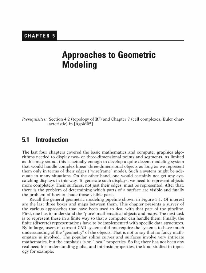
Next, we need to address a problem with the standard Boolean set operators,namely, they are not closed when restricted to r-sets. For example, the intersection ofthe two r-sets X = [0,1] ¥ [0,1] and Y = [1,2] ¥ [0,1] is not an r-set. See Figure 5.4.From the point of view of solids, we would like to consider X and Y as being disjoint.One sometimes calls X and Y quasi-disjoint, which means that their intersection is alower-dimensional set. If we want closure under set operations, we need to revise theirdefinitions.
x y z x y R, , ,( ) + - £{ }2 2 2 0
H f f or H f f+ -( ) = ( ) ≥{ } ( ) = ( ) £{ }p p p p0 0 ,
Figure 5.3. A generic halfspace.
GOS05 5/5/2005 6:20 PM Page 159
160 5 Approaches to Geometric Modeling
Definition. Define the regularized set operators »*, «*, -*, c*, and D* by
where c and D are the complement and symmetric difference operators, respectively.
5.2.1 Theorem
(1) The regularized set operators take r-sets into r-sets. Furthermore, there are algo-rithms that perform these operations.
(2) The class of regular semialgebraic or semianalytic sets is closed under regularizedset operations.
Proof. For (1) see [Tilo80] or [Mort85]. For (2) see [Hiro74].
Even though r-sets are quite general, they have their limitations.
(1) Although they have attractive features from a mathematical point of view, theyare complicated to deal with computationally.
(2) One may want to deal with nonsolids like in Figure 5.2. This is not possiblewith r-sets.
Nevertheless, at least one has something mathematically precise on which to baseproofs.
5.3 Representation Schemes
Geometric modeling systems have taken many different approaches to representinggeometric objects. The following definitions ([ReqV82]) can be thought of as a starttowards being able to evaluate and judge these approaches in a rigorous way.
X Y X Y
X Y X Y
X Y X Y
Y Y
X Y X Y Y X
» = »( )« = «( )- = -( )
= ( )= -( ) » -( )
* ,
* ,
* ,
* ,
* * * * ,
r
r
r
c r c and
D
Figure 5.4. Quasi-disjoint sets.
GOS05 5/5/2005 6:20 PM Page 160

5.3 Representation Schemes 161
Definition. A representation scheme, or simply representation, of a set of “objects” Ousing a set L is a relation r between O and L. If (x,y) Œ r, then we shall say that y rep-resents x. A representation scheme r is unambiguous (or complete) if r is one-to-one.A representation scheme r is unique if r is a function (that is, single-valued). The ele-ments of L are called representations or syntactically correct representations and thosein the range of r are called the semantically correct or valid representations.
See Figure 5.5. The term “syntactically/semantically correct” is used, because if ris a representation scheme, we can think of r(x) as a set of encodings for x in a “lan-guage” L. The semantically correct elements of L are those “sentences” which have a“meaning” in that there is an object that corresponds to them. The terms unambigu-ous and unique separate out those relations that are not many-to-one or one-to-many,respectively. To be unambiguous means that if one has the encoding, then one knowsthe object to which it corresponds. To be unique means that there is only one way toencode an object.
5.3.1 Example. Let O be the set of polygons in the plane that have positive areabut no holes. Let L be the set of finite sequences of points. For example, the sequence(2,1), (-1,3), (4,5) belongs to L. Define a representation scheme for O using L by asso-ciating to each object in O the set of its vertices listed in some order. This represen-tation scheme is neither unambiguous nor unique. It is ambiguous because the objectsin Figures 5.6(a) and (b) both have the same vertices. It is not unique because the ver-tices of an object can be listed in many ways. Furthermore, not all sequences of points
Figure 5.5. Representation scheme.
Figure 5.6. Example of ambiguous repre-sentation scheme.
GOS05 5/5/2005 6:20 PM Page 161

are semantically correct. A sequence of collinear points does not correspond to apolygon in O.
We could modify Example 5.3.1. For example, we could require the polygons tobe convex or we could require that the vertices be listed in counter-clockwise order.In both instances we would then have an unambiguous representation scheme.
There are reasons for why unambiguousness and uniqueness are important prop-erties of a representation scheme. It is difficult to compute properties from ambigu-ous schemes. For example, it would be impossible to compute the area of a polygonwith the ambiguous scheme in Example 5.3.1. An example of why uniqueness isimportant is when one wants to determine if two objects are the same. The ability totest for equality is important because one needs it for
(1) detecting duplication in data base of objects(2) detecting loops in algorithms, and(3) verifying results such as in case of numerically controlled (NC) machines
where it is important that the desired object is created
With uniqueness one merely needs to compare items syntactically. Note that theproblem of determining whether two sets are the same can be reduced to a problemof whether a certain other set is empty, because two sets X and Y are the same if andonly if the regularized symmetric difference XD*Y is empty.
Although unambiguousness and uniqueness are highly desirable, such represen-tations are hardly ever found. Two common types of nonuniqueness are
(1) permutational (as in the example where sequences of points represent apolygon) and
(2) positional (where different representations exist due to primitives that differonly by a rigid motion).
Eliminating these types of nonuniqueness would involve a high computationalexpense.
The domain of a representation scheme specifies the objects that the scheme iscapable of representing. One clearly wants this to be as large as possible. In particu-lar, one would want it to include at the very least all linear polyhedral “solids.” Onealso wants the domain to be closed under some natural set operations such as union,intersection, and difference. This raises some technical issues.
One issue that has become very important in the context of representationschemes is validity.
The Basic Validity Problem for a Representation Scheme: When does a representa-tion correspond to a “real” object, that is, when is a syntactically correct representationsemantically correct or valid?
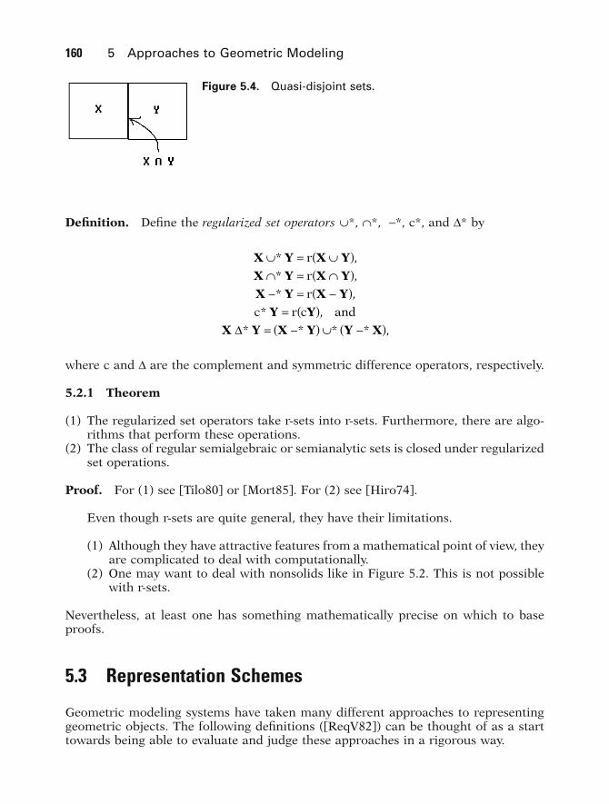
Ideally, every syntactically correct representation should be semantically correctbecause syntactical correctness is usually much easier to check than semantic correctness. Certainly, a geometric database should not contain representations ofnonsense objects. The object in Figure 5.7 could easily be described in terms of surface
162 5 Approaches to Geometric Modeling
GOS05 5/5/2005 6:20 PM Page 162
5.3 Representation Schemes 163
patches and so its definition would seem correct from a local point of view, but takenin its entirety it clearly does not correspond to a real object. In early geometric mod-eling systems, validity of a representation was the responsibility of the user, but thishas changed. It is no longer acceptable to assume human intervention to correcterrors. For one thing, a modeling system might have to feed its geometric data directlyto another system such as a robot and bad data might crash that system.
Here are some other informal properties of representation schemes:
(1) Robustness and numeric precision (see Section 5.10 for a discussion of thistopic)
(2) Compactness (for storing): “Verbose” representations may contain redundan-cies that would make verifying validity harder. On the other hand, in the usualtrade-off, this may improve performance.
(3) Computational ease and applicability: No representation is best for everything.To support a variety of applications, we could have multiple representationsfor each object, but then one must maintain consistency.
(4) Ability to convert between different representation schemes: One may want topass data between different modelers, but even a single modeler may containmore than one representation scheme.
Along with a formalization of the objects that constitute the domain of a modeler,one should also specify and formalize the allowable operations and functions. Thisformalization has only been carried out in a minimal way so far. We postpone thislargely ad hoc discussion to Section 5.7. Insofar as the usual definition of the term“representation scheme” does not address operations and functions, it is an incom-plete concept. The term “object representation scheme” would have been more appro-priate because it is more accurate.
Representation schemes coupled with the user interface of a modeler have a greatinfluence on the way that a user will think about objects or shapes. One needs to dis-tinguish between a machine representation and a user representation. The discussionabove has concentrated on the former, which may or may not be visible to the user,but the latter is also very important and deals with the user interface. A driving forcebehind generative modeling, which will be described in Section 5.3.5, had to do withgiving a modeler a desirable user representation. The issues involved with user rep-resentations are similar to but not the same as those for machine representations.Some important informal questions that a user representation must address are
Figure 5.7. A nonsense object.
GOS05 5/5/2005 6:20 PM Page 163

(1) To what class of shapes is a user restricted?(2) How does a user describe and edit the possible shapes and how easy is this?
(a) How shapes are described can easily limit the user’s ability to use gooddesigns and even to think up a good design in the first place.
(b) How much input is required for each shape?(c) Can a user easily predict the output from the input?(d) How accurate are the representations with respect to what the user wants?(e) Are the operations that a user can perform on shapes closed in the sense
that the output to an operation can be the input to another?
(3) How fast and how realistically can the shapes be generated on a display?(4) What operations can a user perform on shapes and how fast can they be
carried out?
Of course, the type of user representation that one wants depends on the user. Herewe have in mind a more technical type of user. Later in Section 5.6 we consider a userin the context of a manufacturing environment.
5.3.1 Early Representation Schemes
Approaches to geometric modeling have changed over the years. These changes beganbefore computers existed and all one had was pencil and paper. Since the advent of computers, these changes were largely influenced by their power, the essentialmathematics behind the changes being basically not new. As computers become moreand more powerful, it gradually becomes possible to implement mathematical repre-sentations that mathematicians have used in their studies. The history of the devel-opment of geometric modeling shows this trend. Of course, the new ways ofinteractively visualizing data that was not possible before will undoubtedly cause itsown share of advances in knowledge. We shall comment more on this at the end ofthis chapter.
Engineering Drawings. Engineering drawings were the earliest attempts to modelobjects. Computers were not involved and they were intended as a means of com-munication among humans. They often had errors but humans were able to usecommon sense to end up with correct result. There was no formal definition of suchdrawings as a representation scheme. The basic idea was to represent objects by acollection of planar projections. As such it is a highly ambiguous representationscheme because if one were to try to implement it on a computer, it is very difficultto determine how many two-dimensional projections would be needed to completelyrepresent a three-dimensional object. Constructing an object from some two-dimen-sional projections of it is a highly interesting and difficult problem. We touched ontwo small aspects of this problem in Section 4.12. For more, see [RogA90], [BoeP94],[PenP86], or [Egga98].
Wireframe Representations. Wireframe representations were the first representa-tion schemes for three-dimensional linear polyhedra. It is a natural approach, the idea
164 5 Approaches to Geometric Modeling
GOS05 5/5/2005 6:20 PM Page 164
5.3 Representation Schemes 165
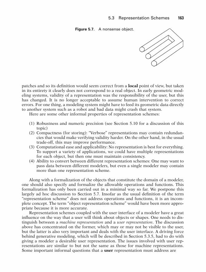
being to represent them using only their edges. After all, edges are some of the mostimportant features of an object that one “sees.” Unfortunately, this representationscheme is ambiguous. For example, Figure 5.8 shows a block with a beveled holethrough its center. It is not possible to tell along which axis the hole lies from the edgeinformation alone. Two problems caused by the ambiguity are that one cannot removehidden lines reliably and one cannot produce sections automatically.
Many early commercially available modeling systems used wireframe representa-tions. Even now many systems support a wireframe display mode because it is fastand adequate for some jobs. A wireframe display is one where only edges and no facesare shown. Note that how objects are displayed is quite independent of how they arerepresented internally.
Faceted Representations. A simple solution that eliminates the major wireframerepresentation problems for three-dimensional objects is to add faces. This represen-tation is unambiguous. We shall look at this approach in more detail later in thesection on the boundary representation. Again, there is a difference between a mod-eling system using a faceted representation and one using a faceted display. The lattermeans that objects (of all dimensions) are displayed as if they were linear polyhedraeven though the system may maintain an exact analytic representation of objects inter-nally. For example, a sphere centered at the origin is completely described by onenumber, its radius, but it might be displayed in a faceted manner.
Attempts have been made to develop algorithms that generate faces from a wire-frame representation automatically, but it is known that only using topological infor-mation leads to an NP-complete problem, so that the algorithms will not be veryefficient in general. See, for example, [BagW95].
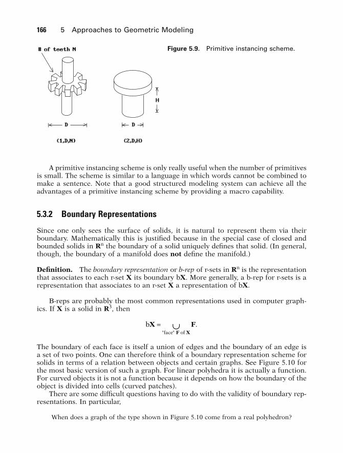
Primitive Instancing Schemes. In this scheme we simply have a finite number ofgeneric parameterized primitives that can be represented via tuples of the form
(type code, parameter 1 , . . . , parameter k)
where the parameters are either reals or integers. See Figure 5.9. We do not need alldimensions as parameters, only those that are variable. The representation is unam-biguous and may be unique. It is certainly very compact. With regard to algorithmsfor computing properties of objects represented by such scheme, one basically needsa special case for each primitive.
Figure 5.8. An ambiguous wireframe representation.
GOS05 5/5/2005 6:20 PM Page 165
166 5 Approaches to Geometric Modeling
A primitive instancing scheme is only really useful when the number of primitivesis small. The scheme is similar to a language in which words cannot be combined tomake a sentence. Note that a good structured modeling system can achieve all theadvantages of a primitive instancing scheme by providing a macro capability.
5.3.2 Boundary Representations
Since one only sees the surface of solids, it is natural to represent them via theirboundary. Mathematically this is justified because in the special case of closed andbounded solids in Rn the boundary of a solid uniquely defines that solid. (In general,though, the boundary of a manifold does not define the manifold.)
Definition. The boundary representation or b-rep of r-sets in Rn is the representationthat associates to each r-set X its boundary bX. More generally, a b-rep for r-sets is arepresentation that associates to an r-set X a representation of bX.
B-reps are probably the most common representations used in computer graph-ics. If X is a solid in R3, then
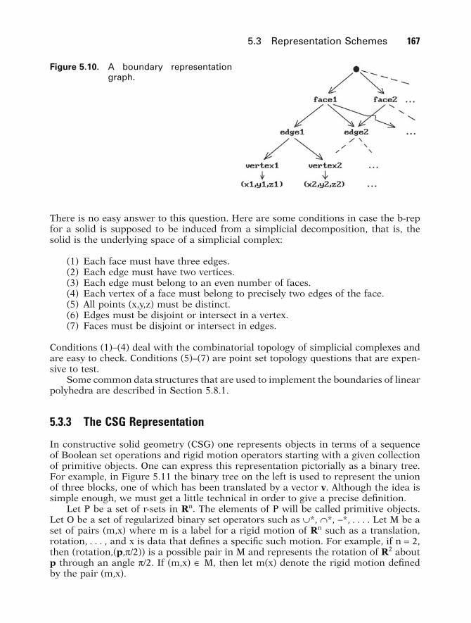
The boundary of each face is itself a union of edges and the boundary of an edge isa set of two points. One can therefore think of a boundary representation scheme forsolids in terms of a relation between objects and certain graphs. See Figure 5.10 forthe most basic version of such a graph. For linear polyhedra it is actually a function.For curved objects it is not a function because it depends on how the boundary of theobject is divided into cells (curved patches).
There are some difficult questions having to do with the validity of boundary rep-resentations. In particular,
When does a graph of the type shown in Figure 5.10 come from a real polyhedron?
bX FF X
= »"face" of
.
Figure 5.9. Primitive instancing scheme.
GOS05 5/5/2005 6:20 PM Page 166
5.3 Representation Schemes 167
There is no easy answer to this question. Here are some conditions in case the b-repfor a solid is supposed to be induced from a simplicial decomposition, that is, thesolid is the underlying space of a simplicial complex:
(1) Each face must have three edges.(2) Each edge must have two vertices.(3) Each edge must belong to an even number of faces.(4) Each vertex of a face must belong to precisely two edges of the face.(5) All points (x,y,z) must be distinct.(6) Edges must be disjoint or intersect in a vertex.(7) Faces must be disjoint or intersect in edges.
Conditions (1)–(4) deal with the combinatorial topology of simplicial complexes andare easy to check. Conditions (5)–(7) are point set topology questions that are expen-sive to test.
Some common data structures that are used to implement the boundaries of linearpolyhedra are described in Section 5.8.1.
5.3.3 The CSG Representation
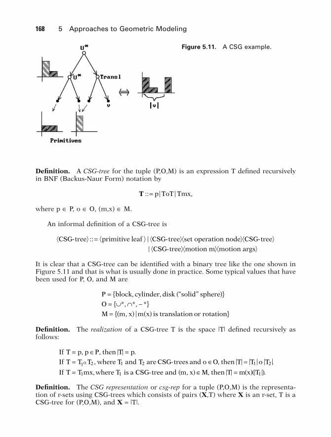
In constructive solid geometry (CSG) one represents objects in terms of a sequenceof Boolean set operations and rigid motion operators starting with a given collectionof primitive objects. One can express this representation pictorially as a binary tree.For example, in Figure 5.11 the binary tree on the left is used to represent the unionof three blocks, one of which has been translated by a vector v. Although the idea issimple enough, we must get a little technical in order to give a precise definition.
Let P be a set of r-sets in Rn. The elements of P will be called primitive objects.Let O be a set of regularized binary set operators such as »*, «*, -*, . . . . Let M be aset of pairs (m,x) where m is a label for a rigid motion of Rn such as a translation,rotation, . . . , and x is data that defines a specific such motion. For example, if n = 2,then (rotation,(p,p/2)) is a possible pair in M and represents the rotation of R2 aboutp through an angle p/2. If (m,x) Œ M, then let m(x) denote the rigid motion definedby the pair (m,x).
Figure 5.10. A boundary representationgraph.
GOS05 5/5/2005 6:20 PM Page 167
168 5 Approaches to Geometric Modeling
Definition. A CSG-tree for the tuple (P,O,M) is an expression T defined recursivelyin BNF (Backus-Naur Form) notation by
where p ΠP, o ΠO, (m,x) ΠM.
An informal definition of a CSG-tree is
It is clear that a CSG-tree can be identified with a binary tree like the one shown inFigure 5.11 and that is what is usually done in practice. Some typical values that havebeen used for P, O, and M are
Definition. The realization of a CSG-tree T is the space |T| defined recursively asfollows:
Definition. The CSG representation or csg-rep for a tuple (P,O,M) is the representa-tion of r-sets using CSG-trees which consists of pairs (X,T) where X is an r-set, T is aCSG-tree for (P,O,M), and X = |T|.
If T p p P then T p
If T T T where T and T are CSG trees and o O then T T o T
If T T mx where T is a CSG M then T m x T
O
= Π== Π== ( ) Π= ( )( )
, , .
, , .
, , .1 2 1 2 1 2
1 1 1
-
-tree and m, x
P solid sphere
O
M m x m x is translation or rotation
= ( ){ }= » « -{ }= ( ) ( ){ }
block, cylinder, disk “ ”
*, *, *
,
CSG tree primitive leaf CSG tree set CSG tree
motion m
- - operation node -
CSG-tree motion args
::=
T :: ,= p ToT Tmx
Figure 5.11. A CSG example.
GOS05 5/5/2005 6:20 PM Page 168
Although one is free to choose any set of primitives or transformations for a csg-rep, generic halfspaces of one sort or another are usually used as primitives. Twocommon csg-reps used
(1) “arbitrary” (possibly unbounded) generic halfspaces as primitives, or(2) bounded generic halfspace combinations as primitives.
Primitives are often parameterized. For example, a primitive block is usually con-sidered to be situated at the origin and to be defined by the three parameters of length,width, and height. One then talks about instancing a primitive, where that term means
(1) assigning values to the configuration parameters, and then(2) positioning the result of (1) via a rigid motion (which could also be viewed as
assigning values to positional parameters).
Csg-reps can handle nonmanifold objects. Their exact domain of coveragedepends on
(1) the primitives (actually the halfspaces which define them),(2) the motion operators that are available, and(3) the set operators that are available.
It is interesting to note the results of an extensive survey of mechanical parts and what it takes to describe them which can be found in [SaRE76]. Fully 63% of all theparts could be handled with a CSG system based on only orthogonal block and cylinder primitives. A larger class of primitives provided a natural description of over90% of the parts. This indicated that CSG is therefore a good fit for a CAD system inthat sort of environment because most mechanical parts seemed to be relativelysimple.
If one uses general operations and bounded primitives, then one gets a represen-tation that is
(1) unambiguous,(2) not unique,(3) very concise, and(4) easy to create (at least for its domain of coverage).
One of the biggest advantages of a csg-rep over other representation schemes isthat validity is pretty much built into the representation if one is a little careful aboutchoosing primitives. For example, if one uses r-sets as primitives and arbitrary regu-larized set operations, then the algebraic properties of r-sets ensure that a represen-tation is always valid. This is not the case if operations are not general, for example,if the union operation is only allowed for quasi-disjoint objects. Also, in a CSG systembased on general generic halfspaces, some trees may represent unbounded sets andhence not be valid. It is true however that, by in large, all syntactically correct CSGrepresentations (trees) are also semantically correct.
Because of the tree structure of a CSG representation, one can often use a divide-and-conquer approach to algorithms: one first solves a problem for the primitive
5.3 Representation Schemes 169
GOS05 5/5/2005 6:20 PM Page 169
170 5 Approaches to Geometric Modeling
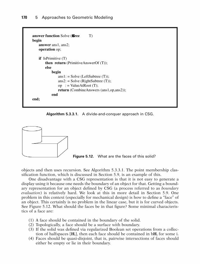
objects and then uses recursion. See Algorithm 5.3.3.1. The point membership clas-sification function, which is discussed in Section 5.9, is an example of this.
One disadvantage with a CSG representation is that it is not easy to generate adisplay using it because one needs the boundary of an object for that. Getting a bound-ary representation for an object defined by CSG (a process referred to as boundaryevaluation) is relatively hard. We look at this in more detail in Section 5.9. Oneproblem in this context (especially for mechanical design) is how to define a “face” ofan object. This certainly is no problem in the linear case, but it is for curved objects.See Figure 5.12. What should the faces be in that figure? Some minimal characteris-tics of a face are:
(1) A face should be contained in the boundary of the solid.(2) Topologically, a face should be a surface with boundary.(3) If the solid was defined via regularized Boolean set operations from a collec-
tion of halfspaces {Hi}, then each face should be contained in bHi for some i.(4) Faces should be quasi-disjoint, that is, pairwise intersections of faces should
either be empty or lie in their boundary.
answer function Solve (CSG-tree T)begin
answer ans1, ans2; operation op;
if IsPrimitive (T) then return (PrimitiveAnswerOf (T));else
beginans1: = Solve (LeftSubtree (T)); ans2: = Solve (RightSubtree (T));op : = ValueAtRoot (T);return (CombineAnswers (ans1,op,ans2));
endend;
Algorithm 5.3.3.1. A divide-and-conquer approach in CSG.
Figure 5.12. What are the faces of this solid?
GOS05 5/5/2005 6:20 PM Page 170
5.3 Representation Schemes 171
Another issue when it comes to faces is how to represent them? We shall see inSection 5.9 that to represent a face F we can
(1) represent the halfspace in whose boundary the face F lies (for example, in thecase of a cylinder, use its equation),
(2) represent the boundary edges of F (the boundary of a face is a list of edges),and
(3) maintain some neighborhood information for these bounding edges andorient the edges (for example, we can arrange it so that the inside of the faceis to the right of the edge or we can store appropriate normal vectors for theedges).
This scheme works pretty well for simple surfaces but for more complicated surfacesone needs more.
5.3.4 Euler Operations
Representation schemes based on using Euler operations to build objects are anattempt to have a boundary representation meet at least part of the validity issue headon. The idea is to permit only boundary representations that have a valid Euler char-acteristic. If we only allow operations that preserve the Euler characteristic or thatchange it in a well-defined way (such operations are called Euler operations), then weachieve this. Of course this is only a part of what is involved for an object not to bea nonsense object. Nevertheless we have at least preserved the combinatorial validitysince the Euler characteristic is a basic invariant of combinatorial topology. As formetric validity, one still must do a careful analysis of face/face intersections. In anycase, to say that a modeler is built on Euler operations means that it represents objectsas a sequence of Euler operations.
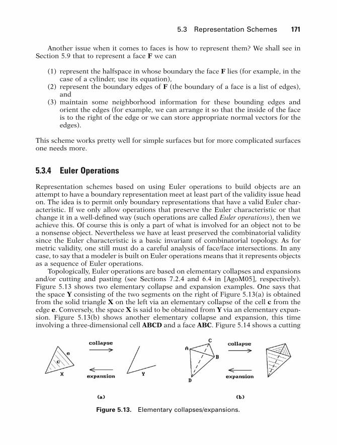
Topologically, Euler operations are based on elementary collapses and expansionsand/or cutting and pasting (see Sections 7.2.4 and 6.4 in [AgoM05], respectively).Figure 5.13 shows two elementary collapse and expansion examples. One says thatthe space Y consisting of the two segments on the right of Figure 5.13(a) is obtainedfrom the solid triangle X on the left via an elementary collapse of the cell c from theedge e. Conversely, the space X is said to be obtained from Y via an elementary expan-sion. Figure 5.13(b) shows another elementary collapse and expansion, this timeinvolving a three-dimensional cell ABCD and a face ABC. Figure 5.14 shows a cutting
Figure 5.13. Elementary collapses/expansions.
GOS05 5/5/2005 6:20 PM Page 171
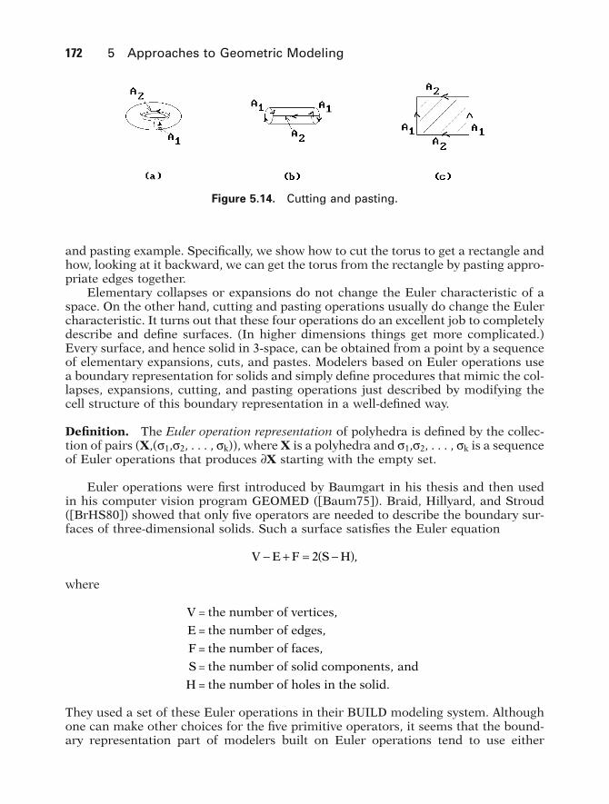
172 5 Approaches to Geometric Modeling
and pasting example. Specifically, we show how to cut the torus to get a rectangle andhow, looking at it backward, we can get the torus from the rectangle by pasting appro-priate edges together.
Elementary collapses or expansions do not change the Euler characteristic of aspace. On the other hand, cutting and pasting operations usually do change the Eulercharacteristic. It turns out that these four operations do an excellent job to completelydescribe and define surfaces. (In higher dimensions things get more complicated.)Every surface, and hence solid in 3-space, can be obtained from a point by a sequenceof elementary expansions, cuts, and pastes. Modelers based on Euler operations usea boundary representation for solids and simply define procedures that mimic the col-lapses, expansions, cutting, and pasting operations just described by modifying thecell structure of this boundary representation in a well-defined way.
Definition. The Euler operation representation of polyhedra is defined by the collec-tion of pairs (X,(s1,s2, . . . , sk)), where X is a polyhedra and s1,s2, . . . , sk is a sequenceof Euler operations that produces ∂X starting with the empty set.
Euler operations were first introduced by Baumgart in his thesis and then usedin his computer vision program GEOMED ([Baum75]). Braid, Hillyard, and Stroud([BrHS80]) showed that only five operators are needed to describe the boundary sur-faces of three-dimensional solids. Such a surface satisfies the Euler equation
where
They used a set of these Euler operations in their BUILD modeling system. Althoughone can make other choices for the five primitive operators, it seems that the bound-ary representation part of modelers built on Euler operations tend to use either
V = the number of vertices,
E = the number of edges,
F = the number of faces,
S = the number of solid components, and
H = the number of holes in the solid.
V E F S H- + = -( )2 ,
Figure 5.14. Cutting and pasting.
GOS05 5/5/2005 6:20 PM Page 172

5.3 Representation Schemes 173
Baumgart’s winged edge representation (see Section 5.8.1) or some variant of it, sothat this is what these operators modify.
Historically, Euler operators were given cryptic mnemonic names consisting ofletters. A few of these are shown below along with their meanings:
Using that notation, three typical operators were:
Figure 5.15 shows how one could create a solid tetrahedron using these operators.The operators create the appropriate new data structure consisting of vertices, edges, faces, and solids and merge it into the current data structure. Along with eachEuler operator that creates vertices, edges, or faces, there are operators that delete orkill them. This enables one to easily undo operations, a very desirable feature for amodeler.
There are good references for implementing modelers based on Euler operations.One is the book by Mäntylä ([Mant88]), which describes a modeling program GWB (the Geometric WorkBench). Another is the book by Chiyokura ([Chiy88]),which describes the modeling program DESIGNBASE. Euler operations were originally defined only for polyhedra but were extended to curved surfaces byChiyokura.
To summarize, modelers based on Euler operations are really “ordinary” b-repmodelers except that the objects and boundary representations that can be built areconstrained by the particular Euler operators that were chosen, so that they at leasthave combinatorial validity. The Euler operators are flexible enough though so that
MEV ---
make ede and vertex
MFE make face and edge
MBFV make body, face, and vertex
M make K kill L - loop
V vertex E edge F face B body solid
- -- - - -S
Figure 5.15. Building a tetrahedron withEuler operations.
GOS05 5/5/2005 6:20 PM Page 173
174 5 Approaches to Geometric Modeling
Figure 5.17. Sweep operations.
the modelers share all the advantages (and some of the disadvantages) that one getswith a boundary representation.
We need to leave the reader, at least those who might be interested in modelingobjects in higher dimensions than three, with one word of caution however. The resultabout five operators sufficing to construct objects raises some subtle issues. It appliesonly to the two-dimensional boundaries of solids and not to cell structures of solids.The fact is that not all n-cells, n > 2, are shellable (another term for collapsible)! Fora proof see [BurM71]. To put it another way, the higher-dimensional analogs of theEuler operators are not adequate for creating all cell decompositions of higher-dimen-sional objects.
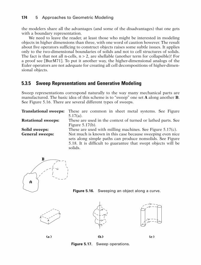
5.3.5 Sweep Representations and Generative Modeling
Sweep representations correspond naturally to the way many mechanical parts aremanufactured. The basic idea of this scheme is to “sweep” one set A along another B.See Figure 5.16. There are several different types of sweeps.
Translational sweeps: These are common in sheet metal systems. See Figure5.17(a).
Rotational sweeps: These are used in the context of turned or lathed parts. SeeFigure 5.17(b).
Solid sweeps: These are used with milling machines. See Figure 5.17(c).General sweeps: Not much is known in this case because sweeping even nice
sets along simple paths can produce nonsolids. See Figure5.18. It is difficult to guarantee that swept objects will besolids.
Figure 5.16. Sweeping an object along a curve.
GOS05 5/5/2005 6:20 PM Page 174

5.3 Representation Schemes 175
Sweeps sometimes become inputs to other representations. For example, in CADD(a program developed by McDonnell Douglas) one can translate certain sweep repre-sentations, such as translational and rotational ones, into boundary representations.
Related to sweeps is the multiple sweeping operation using quaternions describedin [HarA02]. There are also the generalized cylinders of Binford ([Binf71]). See Figure5.19. Here the “sweeping” is parameterized. We shall now discuss a representationscheme developed by J. Snyder at Caltech that is more general yet. It was the basisfor the GENMOD modeling system, which Snyder’s book [Snyd92] describes in greatdetail.
Definition. A generative model is a shape generated by a continuous transformationof a shape called the generator.
Arbitrary transformations of the generator are allowed. There is no restriction asto the dimension of the model. The general form of a parameterization S(u,v) for agenerative model which is a surface is
(5.3)
where g : [a,b] Æ R3 is a curve in R3 and f : R3 ¥ R Æ R3 is an arbitrary function. Oneof the simplest examples of this is where one sweeps a circle along a straight line toget a cylinder. Specifically, let
be the standard parameterization of the unit circle. Define f by
f v vp p, , , .( ) = + ( )0 0
gp p
: ,
cos , sin ,
0 1
2 2 0
3[ ] ÆÆ ( )
R
u u u
S u v f u v, , ,( ) = ( )( )g
Figure 5.18. Problem with sweeps.
Figure 5.19. Generalized cylinder.
GOS05 5/5/2005 6:20 PM Page 175

176 5 Approaches to Geometric Modeling
See Figure 5.20(a). A more interesting example is shown in Figure 5.20(b) where weuse
and Rv is the rotation about the y-axis in R3 through an angle of pv/6. This corre-sponds to sweeping the unit circle along the parabola
in the xz-plane. The circle gets rotated and scaled by a factor of 1 - v/6 as we moveit.
The parameterization S(u,v) in equation (5.3) can be thought of as defining a one-parameter family of curves gv defined by gv (u) = f (g(u),v). As the examples in Figure5.20 suggest, this family of curves can correspond to a fixed curve being operated onby quite general transformations as it is swept along arbitrary curves. This is, in fact,one reason for creating the generative model representation, namely, that it allowspowerful operators for modifying objects.
More generally, generative models of arbitrary dimension have parameterizationS(u,v) of the form
(5.4)
where F : Rk Æ Rm and T : Rm ¥ Rs Æ Rn. This is thought of as a (k + s)-dimensionalmodel obtained by sweeping a k-dimensional object along an s-dimensional path. Forexample, this allows us to define solids as generative models. A common representa-tion is to represent a solid as sweeping an area along a curve.
S R
u v T F u v
k s k s n:
, , ,
R R R¥ = Æ( ) Æ ( )( )
+
z x= - -( ) +13
3 32
f vv
R v xvp p, , ,( ) = -ÊË
ˆ¯ ( ) + - -( ) +Ê
ˈ¯1
60
13
3 32
Figure 5.20. Generative models.
GOS05 5/5/2005 6:20 PM Page 176

Definition. The generative modeling representation consists of pairs (X,F), where Fis a parameterization of the generative model X of the form shown in equation (5.4).
The driving force behind GENMOD was correcting some perceived deficiencies inthe geometric modeling systems of that time and some key defining points listed by[Snyd92] for the generative modeling approach as implemented in GENMOD are:
(1) The representation is a generalization of the sweep representation.(2) Shapes are specified procedurally.(3) Specifying a shape involves combining lower-dimensional shapes into higher-
dimensional ones.(4) An interactive shape description language allows low- and high-level opera-
tors on parametric functions.(5) It is closed, that is, the outputs to operations can be inputs to operations (like
CSG).(6) It allows parameterized shapes whose parameters a user can change.(7) It supports powerful high-level operators and functions, such as
reparameterizing a curve by arc length,computing the volume of a shape enclosed by surface patches, andcomputing distances between shapes.
These operations are closed and free of approximation error.(8) It supports deformation operators, CSG, and implicitly defined shapes.(9) One has the ability to control the error in the representation.
A large variety of symbolic operators on the parameterizations and their coordi-nates help the user define generative models, such as vector and matrix operations,differentiation (partial derivatives), integration, concatenation, and constraint opera-tors. Since parameterizations can be thought of as vector fields, another useful oper-ator is one that solves ordinary differential equations. GENMOD had a language inwhich a user could define models using the various operators.
Now, models will have to be displayed. By converting to polygonal meshes and adhoc error control, the interactive rendering of generative models becomes feasible.One can specify the subdivisions in two ways: uniform in domain or adaptive sam-pling. More realistic images can be obtained at the expense of speed.
For accuracy, GENMOD used interval analysis. Interval analysis (see Chapter 18)is an attempt to make numeric computations on a computer more robust and has itsadvantages and disadvantages. Snyder argued for its use in geometric modeling anddescribed various applications to computing nonintersecting boundaries of offsetcurves and surfaces, approximating implicitly defined curves and surfaces, andtrimmed surfaces and CSG operations on them.
In summary, three more advantages used by Snyder to justify the generative modeling approach are:
(1) The representation handles all dimensions, is high-level, and extensible.(2) Using a high-level interpreted language, the mathematically knowledgeable
user can easily build a library of useful shapes.(3) An adequate number of robust tools for rendering and manipulating genera-
tive models exist.
5.3 Representation Schemes 177
GOS05 5/5/2005 6:20 PM Page 177

5.3.6 Parametric Representations
Many of the representations of solids rest on a representation of their boundaries.That was true even in the case of the csg-rep. Although the primitives were solids, in practice one only had equations or parameterizations for their surfaces, and the interior of the solid was not referenced explicitly. As far as parameterizations areconcerned, there is no reason why we have to limit ourselves to parameterizations of two-dimensional objects. If we want access to interior points, we can define three-dimensional parameterizations just as easily. For example,
is a parameterization of a solid cylinder of radius 1 and height 2 with axis the z-axis.If we allowed such parameterizations, then we could also generate interior points ofthe object at will. Chapter 12 describes a number of basic surfaces and their para-meterizations. Similarly, one could describe a corresponding basic collection of solidsand their parameterizations. In other words, three-dimensional parameterizations area representation scheme for solids. See [Mort85] for a discussion of what he calls atricubic parametric solid. This is a space parameterized by a function p(u,v,w) of theform
This is the most general cubic parameterization, but one can look at special casessuch as Bezier or spline forms, just like in the surface case. See [HosL93].
5.3.7 Decomposition Schemes
Decomposition representation schemes represent objects as a union of quasi-disjointpieces. These representations come in two flavors: object-based or space-based. Theobject-based versions present a subdivision of the object itself. The space-based ver-sions, on the other hand, subdivide the whole space and then mark those pieces thatbelong to the object. The hatched cells in Figure 5.21(b) define a space-based decom-position representation of the object in Figure 5.21(a). Figure 5.21(c) shows an object-based decomposition of the same object.
Another distinction between decomposition schemes is whether they use auniform or adaptive subdivision. The choice is driven by the geometry of the object.For example, at places where an object is very curved it would be advantageous tosubdivide it more to get a more accurate representation. Object-based decompositionschemes tend to be adaptive.
Cell Decompositions. This is a very general object-based decomposition represen-tation. Here the primitive pieces that an object is broken into can be arbitrary (curved)cells, typically triangles in the two-dimensional case or tetrahedra in the three-dimensional one. The idea is to find triangular or tetrahedral pieces each of which
p u v w u v w u v w andijkkji
i j kijk, , , , , , .( ) = Œ[ ] Œ
===ÂÂÂ a a R
0
3
0
3
0
330 1
p r z r r z r z, , cos , sin , , , , , , , ,q q q q p( ) = ( ) Œ[ ] Œ[ ] Œ[ ]0 1 0 2 0 2
178 5 Approaches to Geometric Modeling
GOS05 5/5/2005 6:20 PM Page 178

5.3 Representation Schemes 179
has a relatively simple definition, something that presumably the whole object did nothave. The representation is unambiguous but certainly not unique. Cell decomposi-tions are an essential ingredient of finite element modeling (see Chapter 19).
Certain important topological properties can be computed relatively easily froma cell decomposition, such as answers to the questions
(1) Is the object connected?(2) How many holes does it have?
The representation is also good for nonhomogeneous objects. See Section 7.2.4 in[AgoM04] for a general definition of a cell complex. Handle decompositions of man-ifolds (see Section 8.6 in [AgoM05]) are a special case of this type of representation.Chapter 16 will address the usefulness of “intrinsic” cell decompositions of spaces.
Spatial Occupancy Enumeration. This space-based scheme represents objects bya finite collection of uniformly sized cells. Areas are divided into squares (pixels).Volumes are divided into cubical cells called voxels, an abbreviation for “volume ele-ments.” There are two choices here in that one can either represent the object bound-ary or its interior. In the latter case, one can, for example, list the coordinates of thecenter of grid cells in the object. See Figure 5.22.
Spatial occupancy enumeration is an ambiguous representation. Furthermore, abig problem with this scheme is the amount of data that has to be stored. For that
Figure 5.21. Decompositionrepresentations.
Figure 5.22. Spatial occupancy representation.
GOS05 5/5/2005 6:20 PM Page 179

180 5 Approaches to Geometric Modeling
reason it was not used much for mechanical CAD or CAM (computer-aided manu-facture) initially except for gross models to help with certain calculations such as col-lision checking and getting a rough estimate of volume. This has changed now thatcomputers with gigabytes of memory have become a reality and voxel-based repre-sentation schemes for volumes have become very popular in certain parts of computergraphics. A more detailed discussion of this subject follows in the next section. Section5.8.2 will describe the standard approach to cutting down on the amount of data onehas to store.
5.3.8 Volume Modeling
Here are four terms and their definitions that usually appear in the same context:
Volumetric data: The aggregate of voxels tessellating a volume.Volume modeling: The synthesis, analysis, and manipulation of sampled, com-
puted, and synthetic objects contained within a volumetricdata set.
Volume visualization: A visualization method concerned with the representation,manipulation, and rendering of volumetric data.
Volume graphics: The subfield of computer graphics that employs a volumebuffer for scene representation and is concerned with synthe-sizing, manipulating, and rendering such scenes. Volumegraphics is the three-dimensional counterpart of raster graphics.
The definitions are taken from [KaCY93] and are an adequate representation of howthese terms are usually used. The subject matter that is addressed by these terms iswhat this section is about. It really only dates back to the early 1980s and started inthe context of tomography.
Although our main interest in this book is on modeling geometric objects, volumemodeling covers a much broader subject in that the “volumes” may have arisen inother ways. Volume modeling in its most general sense deals with scalar-valued func-tions defined on three-dimensional space. In that sense, it is not really a modelingscheme per se but has close connections with modeling. In the special case where thefunction takes on only two values, 0 and 1, we can, in fact, interpret the function asdefining a space-based decomposition scheme generalizing the voxel-based spatialoccupancy enumeration scheme. The voxel case is the uniform case, but the data setmay have different geometries such as being composed of rectangular or curved cells.Cells might be different distances apart. On the other hand, the function could comefrom some arbitrary mathematical model. For example, one might want to displaythe temperature of a heated solid visually, perhaps by displaying the surfaces of con-stant temperature. We can think of volume modeling as modeling data that is acquiredfrom appropriate instruments and then sampled to get the voxelization. The datacould also be an “object” that is defined in terms of point samples. Volume renderingrefers to the process of displaying such models. We shall have more to say aboutvolume rendering in Section 10.4.
GOS05 5/5/2005 6:20 PM Page 180

5.3 Representation Schemes 181
Volume modeling is beginning to make an impact on the more conventional CADand CAGD. Here are some of its advantages:
(1) One can “cut away” parts of an object and look at its interior. See Figure 5.23.(2) CSG can be implemented quite easily because at the voxel level the set oper-
ations are easy, especially if one has support for voxBlt (voxel block transfer)operations that are the analog of the bitBlt operations.
(3) Rendering is viewpoint independent.(4) It is independent of scene and object complexity.
The author has felt for many years that it was advantageous to model the whole worldand not just the objects within it. It gives one much more information. For example,to trace a ray, one simply marches through the volume and sees what one hits alongthe way, rather than having to check each object in the world for a possible intersec-tion. Volume modeling is now making this possible.
Some disadvantages of volume modeling are:
(1) A large amount of data has to be maintained.(2) The discretization causes loss of information.(3) The voxelization causes aliasing effects.
Volume modeling plays an important role in the visualization of scientific data.This is a big field in computer graphics. Although not the focus of this book, it wouldnot be right to omit mentioning some examples of it:
Medical Imaging. This was one of the first applications of volume modeling. See[StFF91] for an overview of early work. Physicians used MRI (magnetic resonanceimaging) and CT (computed tomography) scanners to get three-dimensional data ofa person’s internal organs. In tomography one gets two-dimensional slices of theobject using X-rays. One projects X-rays through the body and measures their inten-sity with detectors on the other side of the body. The X-ray projector is rotated aboutthe body and measurements are taken at hundreds of locations around the patient. A
Figure 5.23. Foot with bones exposed([ScML98]). (Reprinted from Schroeder et al: The Visualization Toolkit: An Object-OrientedApproach to 3D Graphics, third edition, 2003, 1-930934-07-6, by permission of the publisherKitware Inc.).
GOS05 5/5/2005 6:20 PM Page 181

picture of the slice is then obtained from a reconstruction process applied to all thisdata. Radiologists were apparently good at seeing three-dimensional models fromthese two-dimensional slices, but surgeons and doctors were not. Fortunately, thereexist algorithms that, when applied to a stack of such slices, produce a representationof the whole organ and volume rendering makes it possible to display it. One is ableto remove uninteresting tissues to see those parts that one wants to see. At this pointin time, three-dimensional medical graphics is not yet widely used, mainly becauseof the cost. Also, the slices are more accurate and have more information than thethree-dimensional reconstruction, so that radiologists tend to refer to them more.
In another recent development, surgeons can now also use haptic systems to prac-tice surgeries beforehand. “Haptic” means that one gets physical touch feedback fromthe system.
Modeling Natural Phenomena. Understanding the flow of air over an airplanewing is important for its design. A similar understanding is needed for designingintake or exhaust manifolds in engines. This is where fluid dynamics enters. Fluiddynamics deals with fluid flow, which is governed by a set of differential equationscalled the Navier-Stokes equations. These equations define the velocity and vorticityof the fluid. The vorticity describes the rotational part of the flow and is defined by a vector at each point of the fluid. Understanding vector-valued functions is not easy, but volume-rendering techniques have enabled scientists to get a better visualunderstanding of what happens inside a flow. Volume modeling has been helpful in modeling other phenomena such as ocean turbulence and hurricanes. Oil explorationhas been greatly aided by the ability to use volume modeling to analyze geologicaldata.
Education. Volume modeling has been used to avoid having to use actual bodies indissection experiments. As a result of the visible human project sponsored by theNational Library of Medicine, there now exist models of a human male and female.If one tried to model a human in the more traditional way by means of facets, it wouldtake millions of triangles to do so.
Nondestructive Testing. Volume modeling has been used to enable mechanical andmaterials engineers to find structural flaws in objects without having to take themapart.
This ends our brief overview of volume modeling. We return to the very interest-ing topic of volume rendering in Section 10.4. There is a large body of literature onvolume modeling and the related subject of scientific visualization. A good place tobegin more reading is [LiCN98], [ScML98], and various ACM SIGGRAPH course notessuch as [Kauf98].
5.3.9 The Medial Axis Representation
In mathematics, when one tries to characterize or classify geometric objects, one firstlooks for coarse invariants (topology) and then successively refines the classificationby adding metric criteria, differentiability criteria, etc. For example, at a very top level,
182 5 Approaches to Geometric Modeling
GOS05 5/5/2005 6:20 PM Page 182
5.3 Representation Schemes 183
a doughnut and a circle are similar because one can collapse the doughnut down toa circle. A double doughnut (two doughnuts attached to each other along a disk) islike a figure-eight curve. Therefore, since the circle is clearly a quite different shapefrom a figure-eight, one can see that the more complicated solids to which they areassociated must also be fundamentally different shapes. This section is about a similaridea, namely, to facilitate dealing with objects by representing them by simpler (lower-dimensional) objects that nevertheless still capture the essence of the shape of theoriginal object. The idea of using a “skeleton” of an object as a shape descriptor goesback to [Blum67] and [Blum73]. The fact that one gets a representation that has manyattractive features has led to quite a bit of research activity on this subject. It shouldbe noted, however, that the skeletal representation of an object is not a stand-alonerepresentation for objects in practice. Mostly, it is intended to be used in conjunctionwith others, typically a boundary representation for continuous objects and a spatialoccupancy enumeration representation based on pixels or voxels for discrete objects.
Skeletons come in two flavors, namely, continuous and discrete. We shall beginwith definitions for the continuous case.
Definition. Let X Õ Rn. A maximal disk in X is a closed disk Dn(p,r) contained in Xwith the property that it is not properly contained in any other closed disk in X.
Definition. Let X Õ Rn. The medial axis (MA) or skeleton or symmetric axis of X isthe closure of the set of centers of maximal disks in X. The medial axis of a solid inR3 is sometimes called a medial surface. The real-valued function that assigns to eachcenter of a maximal disk in X the radius of that disk extends to a continuous func-tion on the medial axis called the radius function of that medial axis.
Note. Unfortunately, there is not complete agreement with regard to the termsmedial axis, skeleton, and symmetric axis in the literature. For example, the medialaxis in the continuous case is often also defined as the set of points equidistantlyclosest to at least two points in the boundary. The advantage of the definition givenhere with its closure condition is that if X is bounded then the medial axis will be acompact set.
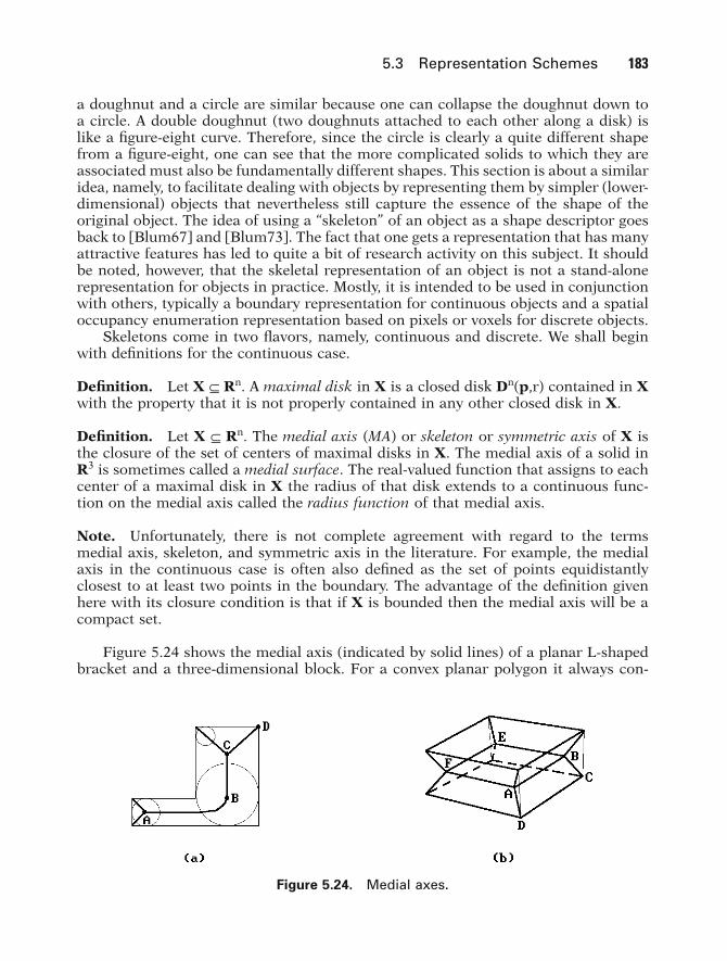
Figure 5.24 shows the medial axis (indicated by solid lines) of a planar L-shapedbracket and a three-dimensional block. For a convex planar polygon it always con-
Figure 5.24. Medial axes.
GOS05 5/5/2005 6:20 PM Page 183
184 5 Approaches to Geometric Modeling
sists of straight line segments but if the polygon is nonconvex there may be curvedarcs as Figure 5.24(a) shows. There is a close relation between the medial axis andthe Voronoi diagram of an object ([ShAR96]).
The medial axis for a polyhedron has a natural partition into cells. Determiningthe medial axis basically reduces to determining its cell decomposition. In two dimen-sions the cells are called arcs and junctions. For example, in Figure 5.24(a) BC andCD are arcs and the points A, B, and C are called junctions. In the nondegeneratecase, junctions are the points where the maximal disk has three or more contact pointswith the boundary. The maximal disks at endpoints of arcs that lie in the boundary,like point D, have one contact point with the boundary. In three dimensions the cellsare called sheets, seams, and junctions. The sheets are surface patches. These arefurther subdivided into wing sheets and body sheets. Wing sheets are those with pointsin their boundary where the maximal disk makes contact with the boundary at onlyone point, such as ABCD in Figure 5.24(b). Body sheets are the remaining sheets,such as ABEF. The seams are curves that typically are the intersection of two or moresheets where the maximal disk has three or more contact points with the boundary.Junctions are points that are the intersections of three or more sheets. See [BBGS99].
Next, consider discrete objects. We could give the same definitions because all thatwe need is a metric which we have. However, there are several natural metrics tochoose from in this case and so it is possible to play around with the definition a bitand choose a variant which may be more suitable for a particular discrete problem.We follow [RosK76].
Definition. Let X Õ U Õ Zn. The medial axis (MA) or skeleton or symmetric axis ofX with respect to U is the set of points whose distances from the complement U - Xare a local maximum, that is, no neighboring point has a greater distance to the com-plement. The distance function for the medial axis is the real-valued function thatassigns to each point of the medial axis its distance to U - X.
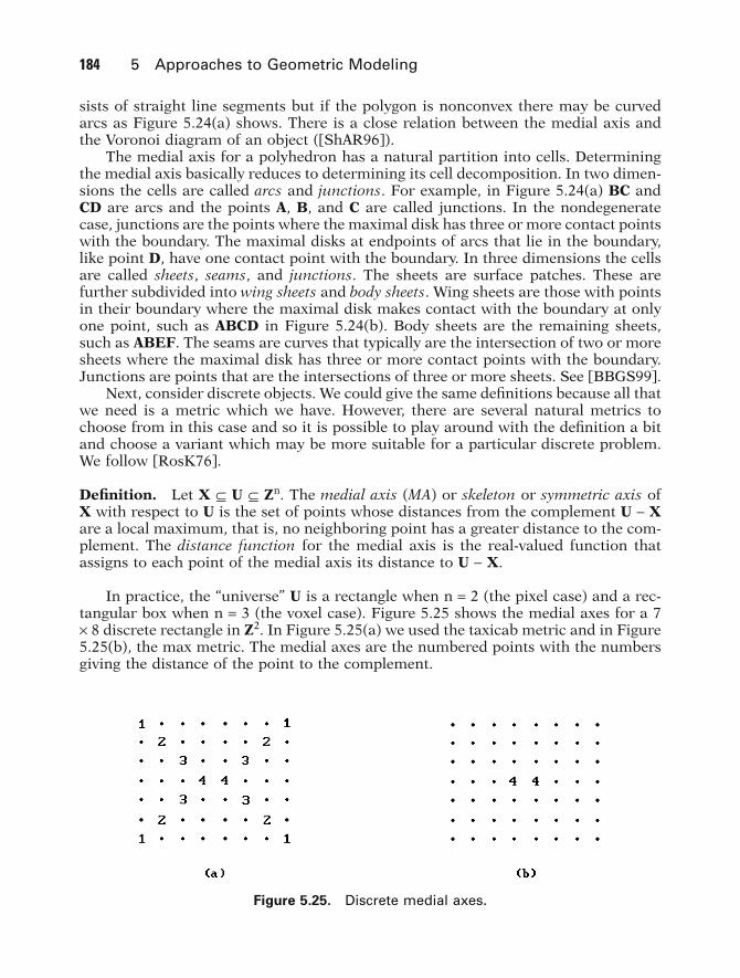
In practice, the “universe” U is a rectangle when n = 2 (the pixel case) and a rec-tangular box when n = 3 (the voxel case). Figure 5.25 shows the medial axes for a 7¥ 8 discrete rectangle in Z2. In Figure 5.25(a) we used the taxicab metric and in Figure5.25(b), the max metric. The medial axes are the numbered points with the numbersgiving the distance of the point to the complement.
Figure 5.25. Discrete medial axes.
GOS05 5/5/2005 6:20 PM Page 184

Definition. The medial axis representation or medial axis transform (MAT) of anobject consists of its medial axis together with the associated radius function in thecontinuous case and the distance function in the discrete case.
One can show that an object is completely specified by its medial axis represen-tation. See [Verm94] and [RosK76]. Furthermore, in the continuous case the enve-lope of the maximal disks is just the boundary of the object. One nice thing about themedial axis representation is that it depends on the geometry of the object and noton the choice of coordinate axes like the quadtree or octree representation for dis-crete objects defined by pixels or voxels.
Algorithms that compute medial axes divide into two types based on whether theyapply to discrete or continuous objects. The basic thinning algorithm for computingthe discrete medial axis is often referred to as the “grassfire” algorithm. If a firestarted at the boundary of the object were to burn into the object at a constant rate,then it would meet in the medial axis. One starts on the boundary of the object andstrips away one layer of pixels or voxels after another until one reaches points thatthe fire reaches from two directions. See [RosK76] and [WatP98] for thinning of two-dimensional discrete sets. Similar arguments work in three dimensions.
In describing algorithms for finding the medial axis of continuous objects we shallconcentrate on three-dimensional objects. Such algorithms can be classified by thespecific approach that is used: volume thinning, tracing of seams and sheets, Voronoidiagrams, or Delaunay triangulation. See [BBGS99] for advantages and disadvantagesfor various schemes. [CuKM99] also describes previous work.
Volume Thinning. One voxelizes the object and then computes the discrete medialaxis that is then polygonized. An additional extra pass is required at the end to deter-mine the radius function. Of course, this will only determine an approximation to themedial axis and one must be careful that it is accurate.
Tracing Approaches. One tracing approach is described in [ShPB95]. One starts ata known junction like a vertex of the polyhedron and then traces along an adjacentseam, defined as the zero set of some functions, until one gets to another junction. Atthat point one repeats this process for each seam that ends at that new junction. Polyg-onal approximations to the seams are computed. The main difficulty is determiningthe next junction. A similar approach is used in [CuKM99] but is claimed to be moreaccurate because it uses exact arithmetic.
Voronoi Diagrams. A number of algorithms use Voronoi diagrams because of theirclose connection to the medial axis problem since they also deal with equidistant setsof points. See Section 17.7 for a definition of Voronoi diagrams and some of theirproperties. The idea is to use a suitable sample of points in the boundary and computetheir Voronoi diagram. See [Bran92], [ShPB95], or [ShPB96]. [CuKM99] describes analgorithm for polyhedra via Voronoi diagram and exact arithmetic.
Delaunay Triangulations. See Section 17.8 for a definition of a Delaunay triangu-lation of a set of points. A Delaunay triangulation is the geometric dual to the Voronoidiagram. [ShAR95] and [ShAR96] generate a domain Delaunay triangulation con-sisting of a set of tetrahedra based on an adaptive collection of boundary points. Themedial axis is obtained from this triangulation.
5.3 Representation Schemes 185
GOS05 5/5/2005 6:20 PM Page 185

186 5 Approaches to Geometric Modeling
Most algorithms are basically discrete algorithms. One exception is the algorithmdescribed in [Hoff94] for CSG objects. In this regard, see also [LBDW92]. The authorsdescribe how one can obtain an approximation to a variant of the Voronoi diagramfor CSG objects. Sometimes bisectors of surfaces are rational. See [ElbK99]. In caseof polyhedra, the medial surface consists of bisectors that are planes or quadric sur-faces. An algorithm for planar regions with curved boundaries can be found in[RamG03].
To use the medial axis representation effectively one needs to know not only howto compute it but also how one can reconstruct the original object from it. The lattertask is often referred to as refleshing. Algorithms for refleshing divide into direct andimplicit approaches.
The direct approach to refleshing tries to reconstruct the boundary surface ofthe original object directly using the given radius or distance function. This amountsto constructing the surface from a variable offset type surface. See [GelD95]. Self-intersections are a problem with offsets and the exterior skeleton has been used hereto help prevent these. See [STGLS97]. The exterior skeleton or exoskeleton of an objectis the skeleton of the complement of the object. The ordinary skeleton is sometimescalled the interior skeleton or endoskeleton. The exterior skeleton comes in handy atthose places where the boundary of the object is concave. See Figure 5.26.
The implicit approaches to refleshing try to define the boundary surface implic-itly as the zero set of a suitable function. They can be further subdivided into thosethat use a distance function and those that use convolution methods. See [BBGS99]for a more detailed discussion of this along with references. The paper also describesa new distance function approach. This involves triangulating the medial axis anddefining a local distance function for each triangular facet. The global distance func-tion is then the minimum of all the local ones. To give the reader a flavor of how alocal distance function is constructed, we sketch the construction in the case wherethe radius function is constant over a facet. The local distance function is a compos-ite of functions defined over regions that are related to the Voronoi cells associatedto the facet, its edges, and its vertices. See Figure 5.27, which shows a triangular facetwith vertices p1, p2, and p3 and its associated Voronoi cells whose boundaries areobtained by sweeping a vector orthogonal to the edges of the facet orthogonally to theplane of the facet. Let fsi be the local distance function for point pi determined by the
Figure 5.26. Interior and exterior skeletons.
GOS05 5/5/2005 6:20 PM Page 186

5.3 Representation Schemes 187
sphere labeled spherei. Let fcylij be the local distance function associated to the cylin-der labeled cylij that is centered on the edge from pi to pj and meets the sphereslabeled spherei and spherej tangentially. Let fplanes be the local distance function asso-ciated to the planes that meet the spheres labeled spherei tangentially. Then the localdistance function f(p) associated to the facet is defined by
If the radius is not constant over a facet but varies linearly over it, then a similar con-struction works using cones rather than cylinders. In the end, the refleshed object isdefined as the halfspace of a (distance) function. The implicitly defined boundary (thezero set of the function) can then be polygonized by some standard method if this isdesired.
One goal of the medial axis representation is to make modeling easier for the user.For one thing, we have reduced the dimension by one. An example of this is the rep-resentation of an object by orthogonal projections. See [Bloo97], [STGLS97], and[BBGS99] for how a user might edit an object using its medial axis. In [BBGS99] thebasic approach to editing a solid was
(1) Compute the medial axis and radius function for the solid.(2) Allow the user to interactively edit the skeleton and radii.(3) Reflesh to obtain the edited solid.(4) Polygonize the boundary of the solid so that the user can use the b-rep for
other purposes.
The allowed editing operations were
(1) Stretching: The user picks skeletal vertices and a translation vector.(2) Bending: The user picks a joint and specifies a rotation by clicking with the
mouse on one side of a separating plane through the rotation axis.(3) Rounding: At sharp convex edges the wing sheets meet the boundary of the
object and the disk radii go to zero. The user can either remove the wing sheetsor change the disk radii.
f f if sphere labeled sphere
f if cylinder labeled cyl
f if region labeled planes
si
cylij
planes
p p p i
p p ij
p p
( ) = ( ) Œ= ( ) Œ= ( ) Œ
,
,
, .
Figure 5.27. The regions used to define a localdistance function for a facet.
GOS05 5/5/2005 6:20 PM Page 187
(4) Editing disk radii: This allows a user to round, thicken, or thin parts of theobject in uniform or nonuniform ways.
The bending operation in particular shows why the medial axis representation has anadvantage over a b-rep. With a b-rep such an operation can produce tears if one isnot careful. Although bending the medial axis may produce tears or intersections, therefleshing operation removes all that.
Medial axis computations have many applications. Just to list a few topics andreferences, they are used in finite element mesh generation ([STGLS97]), shape opti-mization and robot path planning ([GelD95]), and pattern analysis and shape recog-nition ([FarR98]). See [Nack82] for relationships between the curvature of a surfaceand curvature functions associated to its medial axis representation.
Finally, related to the medial axis are the level sets of [LazV99] and the Reebgraph of [ShKK91] and [ShiK91]. With level sets the goal was to describe both thetopology and geometry of the object, whereas with the Reeb graph the goal was toencode the topology. Both of these approaches are based on the handle decomposi-tion of manifolds that is central to the classification of manifolds. See Chapter 8 in[AgoM04]. Reeb graphs have also been useful for volume data mining ([FTAT00]).
5.4 Modeling Natural Phenomena
Except for the pixel- and voxel-based types, the representation schemes we have dis-cussed so far are not very useful for modeling natural phenomena. Objects such astrees, mountains, grass, or various terrain cannot easily be modeled by linear poly-hedra or smooth surface patches. Using very small pieces in the representation wouldoverwhelm one with massive amounts of data. Even if this were not a problem, itwould not be a satisfactory solution. The picture might look all right at the start, butwhat if one were to zoom in? One would have to adjust the fineness of the subdivi-sion dynamically to prevent things from eventually looking flat. Modeling and ren-dering natural phenomena is a digression from the main thrust of this book. For thatreason, we shall only take a brief look at this subject. The four topics we consider arefractals, iterated function systems, grammar based models, and particle systems.
Fractals. One of the most important applications of fractals to graphics is in therepresentation of natural phenomena. For a definition of a fractal, see Section 22.3.They enable one to represent such phenomena in a realistic way with a small amountof data. The zooming problem also is no problem here. There is one caveat however.Fractals are typically used to represent “generic” trees, mountains, or whatever. Theydo not lend themselves easily to represent a specific tree or mountain. This is usuallynot an issue though.
Why are fractals so great for modeling certain natural phenomena? To begin withlet us show how fractal curves and surfaces can be generated. The basic constructiongeneralizes that of the well-known Koch curve (see Section 22.3).
In the one-dimensional case, the algorithm starts with a given initial polygonalcurve and then generates a sequence of new curves, each of which adds more detailto the previous one. In every iteration we replace each segment of the old curve with
188 5 Approaches to Geometric Modeling
GOS05 5/5/2005 6:20 PM Page 188

5.4 Modeling Natural Phenomena 189
a new curve segment. The simplest way to do this is to displace the midpoint of thesegment by a random amount along the perpendicular bisector. See Figure 5.28. Giventhe segment AB, let C be its midpoint. Compute a unit normal vector u for it, choosea suitable random number r based on the current scale, and replace AB by the seg-ments AD and DB, where C is the midpoint of AB and D = C + ru.
Now, to describe some natural shape such as the boundary of an island proceedas follows: Specify the rough outline of island with a polygonal curve and then applythe algorithm described above, that is successively replace each edge with an appro-priate collection of edges. Figure 5.29 shows one possible result after starting with anapproximation to the Australian continent. One does have to deal with the problemof self-intersections in the resulting curves.
In the two-dimensional case, we have more freedom. For example, for surfacesdescribed as a collection of triangles one common approach is to do the following:“Subdivide” each triangle into smaller triangles obtained by connecting its vertices toappropriate random offsets of the midpoints of its sides. This replaces each trianglesuccessively by seven new smaller triangles and the process can be repeated. In Figure5.30(a) the midpoints of the edges of triangle ABC were offset to D, E, and F, and thetriangle replaced by triangles ABD, BDE, BEC, CEF, ACF, ADF, and DEF. A similarconstruction works for quadrilaterals. There is one complication in the two-dimensional case, namely, if one is not careful, then gaps can appear in places wheretriangles used to be adjacent. Figure 5.30(b) shows the potential problem if we offset
Figure 5.28. Curve midpoint displacements.
(a) Rough sketch (b) After random subdivisions
Figure 5.29. A fractal island.
GOS05 5/5/2005 6:20 PM Page 189

190 5 Approaches to Geometric Modeling
the midpoint of the edge AB to X and X¢ with respect to the triangles ABC and ABC¢,respectively. One has to make sure that one uses the same random number and normalwhen offsetting an edge with respect to both triangles that have it in common.
Some good references on fractals are [Mand83] and [DevK89].
Iterated Function Systems. Iterated function systems are an elegant way to gen-erate fractals. We refer the reader to Section 22.4 for a brief discussion. [Barn88] isa good reference.
Grammar-Based Models. Building on work of Lindenmayer ([Lind68]) on parallelgraph grammars, Smith ([Smit84]) described a class of plant models that he calledgraftals. The modeling involved two stages: first one generates a formal string froman initial string using production rules and then the image is generated by interpret-ing this string as a geometric tree in a suitable way. Graftals were not necessarily frac-tals, but were very similar in that one could generate as much detail as desired. Veryrealistic plants and trees could be generated using botanical laws.
Particle Systems. Particle systems, introduced in [Reev83], were good at modelingphenomena that was “fluid-like” and changed over time by flowing or spattering, suchas clouds, smoke, fire, water falls, and water spray. Typical particles were spheres andellipsoids. They would be created in a random way with respect to size, position,shape, and other properties and then randomly deleted. During their lifetime theirpaths, which could be controlled by specified physical forces, would be rendered inappropriate colors. See also [ReBl85].
Most models above are what are called procedural models. We have more to sayabout this later in Sections 5.6 and 5.11.
5.5 Physically Based Modeling
The kind of modeling we have discussed so far has dealt mostly with static objects.Allowing for animation would not change that since animation is nothing but a matterof generating a sequence of views of static objects (rather than a single view). Thisstatic modeling is what the traditional CAD systems do and is quite adequate in aiding
Figure 5.30. Surface midpoint displacements.
GOS05 5/5/2005 6:20 PM Page 190
users in the tasks for which they are used. The real world does not consist of isolatedobjects however. Objects interact due to a variety of forces. We need to broaden ouroutlook. Another goal should be to facilitate the modeling of the real world with itsinteractions. Geometric modeling, the modeling of isolated static objects, is an impor-tant step toward modeling real world scenes, but it is only a first step. The next stepis to make it easier for users to include the interactions of the objects.
For example, if we wanted to model a ball in a scene with a cloth draped over it,we could do it with the standard modeling system, but it would take quite some effort.We would have to figure out the creases in the cloth on our own. These creases aredetermined by gravity and other physical forces associated to the particular materialfrom which the cloth is made. We could use the relevant equations of physics to definethe set of spline surface patches, or whatever, that would generate the correct picture.How much easier it would be if we only had to tell the CAD program the position andradius of the ball, the material properties of the flat cloth, the starting position of thecloth parallel to the floor at the top of the ball, and then let the program compute thefinal shape of the cloth after it has reached equilibrium with respect to the forcesacting on it. Obviously, a program that could do this would have to have the relevantequations and algorithms programmed within it, but this would only have to be doneonce.
As another example, suppose that we wanted to show a ball bouncing on a floor.Again, we could do this animation ourselves with a traditional CAD system by deter-mining by hand the series of positions of the ball along with the time intervals betweenthose positions that made up the animation. Why can the CAD program not do thisfor us, so that all we had to input was an initial height from which the ball is dropped?Obviously, the CAD system could be programmed to do this. This would take somehard work, but again, it would only have to be done once, and then it could help manyusers in this and similar types of problems.
Modeling that also considers the dynamics of physical objects in addition to theirstatic properties is called physically based modeling. The objects may be simple parti-cles or rigid objects, but could also be much more complex, like cloth. As indicatedearlier, we are not really dealing with a new representation scheme but rather anextension of “traditional” representation schemes. This is a relatively new branch ofcomputer graphics, with the name “physically based modeling” being introduced forthe first time in an ACM SIGGRAPH 87 course by A.H. Barr ([BarrA87]). To carry outits program involves a great deal of knowledge about physics and other sciences.
Physically based modeling can be interpreted quite generally to encompass thethree main areas in computer graphics, modeling, rendering, and animation, but atits core, it deals with classical dynamics of rigid or flexible bodies, interaction ofbodies, and constraint-based control. An active area of research is how a user can bestcontrol the models. There is a trade-off between realism and control. If the modelsperform realistically, they are typically controlled by differential equations and theonly control a user has in initial conditions. On the other hand, giving the user morecontrol might mean that objects will perform less realistically. Constraint-based tech-niques are a common way to deal with this problem. This includes constraints definedby equations in physics but also refers to situations where we would like the user tobe able to say things like “move object A so that it touches both objects B and C,” “leta ball roll down a hill following a given path,” or “show a moving robot, figure, orobject in a domain with obstacles.” Unfortunately, if constraints are not chosen care-
5.5 Physically Based Modeling 191
GOS05 5/5/2005 6:20 PM Page 191

fully, we may create underconstrained situations where there is no unique solution,or overconstrained situations where there is no solution.
For a more thorough discussion of physically based modeling see the referencesin that section of the bibliography.
5.6 Parametric and Feature-Based Modeling
We have mostly talked about various technical aspects of modeling systems, but agood modeler must also take the user’s or designer’s point of view into account. Thedifference between a machine representation and a user representation was brieflyalluded to in Section 5.3. We also touched on this subject in our discussion of gener-ative modeling in Section 5.3.5. Users should not have to be forced to adapt their wayof describing geometry to any low-level abstractions due to technical requirements ofa modeler. Defining nontrivial geometric models is usually a difficult task in the bestof circumstances. If possible, the process should require no more expertise than theunderstanding of the final model. Of course, there are times when knowing the under-lying mathematics is essential to building a model and so the option of taking advan-tage of it should be there. Nevertheless, for those times when it is not, we would likea modeler to have the ability to understand high-level, user-friendly concepts. Ofcourse, what is considered user friendly depends on the user. In this section we areconcerned with manufacturing environments, where, for example, designers oftenthink of geometric objects in terms of important features that are associated to them,such as, “a block with a slot and rounded corners.” Today’s modelers have a long wayto go in fully supporting that type of interface. This section will introduce the readerto what is referred to as feature-based modeling. [ShaM95] is a good reference for thissubject. A brief survey can be found in [SodT94].
Systems using parametric or variational models were a first step toward feature-based modeling and making life easier for the designer. As is pointed out in [ShaM95],perhaps 80% of new designs are simply variations of old ones. Therefore, given theeffort that is sometimes needed to create an individual model, why should one haveto create each of these variants from scratch? As an oversimplified example of the typeof interface that would be found in a modeler using parametric models, the object inFigure 5.31 might be defined by the following sorts of commands:
192 5 Approaches to Geometric Modeling
Figure 5.31. A parametric model.
GOS05 5/5/2005 6:20 PM Page 192

5.6 Parametric and Feature-Based Modeling 193
(1) horizontal line A of length a(2) line B perpendicular to line A of length b(3) line D makes signed angle a with line B(4) circular arc C tangent to lines A and D
It would then be up to the system to check if this description gives rise to a uniqueconsistent model for particular values of a and b. The basic design process in such a modeling system is then that the user describes a list of geometric primitives to be used and the geometric relationships between them symbolically without anynumbers. After the user inputs the actual geometric constraints, the system createsan actual instance of the object if possible. The user can subsequently input new dataand get new instances of the object. Note that the “parametric” models consideredhere are higher-level constructs than those in the generative representation discussedin Section 5.3.5.
Although the terms “parametric” and “variational” are often used interchangeably,there is a subtle distinction between what are called parametric and variationalmethods. Parametric methods solve constraints by replacing symbolic variables byvalues that are computed sequentially from previously computed variables. Varia-tional methods use equations to represent constraints and solve them simultaneously.The difference is captured by the difference between defining a variable via a formulaor implicitly. For more on parametric and variational modeling see [ShaM95]. Somesample papers on constraint-based modeling with additional references are [LiHS02]and [Podg02].
An approach to geometric design based on functional programming that extendsvariational modeling is described in [PaPV95]. The authors discuss a high-level func-tional programming language (a language that manipulates functions) with the under-lying geometric objects represented in a hierarchical manner much like in CSG.Elementary polyhedra are stored as inequalities and the basic Boolean set operationsare supported. The language is such that all syntactically correct objects are valid. Itis argued that the power of this functional approach is that it lets the user naturallygenerate new models from old ones and is similar to generative modeling in thisrespect.
Parametric and variational modeling is a start toward facilitating geometricdesign, but it still only deals with individual geometric primitives with no groupingcapabilities and lacks a vision of the whole modeling process. Consider a manufac-turing company. Its ability to deal with the design, planning, and manufacturingprocess in an integrated way is clearly of practical importance. To do this one needsto model the whole process. However, the models used by a designer should be allowedto be different from those used by the person manufacturing the product about whichthe designer may know little. Both may evolve over time and one only needs a way tomap from one to the other. Feature modeling seems like a promising approach to anintegrated solution. Again, the problem with the type of modelers we have been dis-cussing up to now is that they dealt solely with the geometry of objects and ignoredmany of the other issues such as process planning, assembly planning, and inspec-tion planning. Even in the case of just the geometry they were not totally adequatesince they tended to be low-level and did not make it easy for a designer to makechanges, although parametric modeling helped.
GOS05 5/5/2005 6:20 PM Page 193

Feature-based modeling dates back to the mid-1970s when attempts were madeto get data on manufacturing features for NC programming. Kyprianou [Kypr80] was the person who first introduced automated feature recognition into a modeler(BUILD). [PraW85] was one of the earliest studies of “design by features.” So whatexactly is a “feature?”
The term “feature” refers to a high-level abstract entity. It refers to some inter-esting aspect of, or associated to, an object and is usually a combining of details intoone entity that is more meaningful for manipulation than the individual parts. Forexample, in a b-rep modeler a block with a hole through it might consist of a collec-tion of surface patches with no explicit notion of the center and radius of the hole.Moving the hole might then involve moving and changing a subset of these patches –a tedious task. The term “feature” was first used in manufacturing but has since takenon a broader meaning. Machined parts typically can be described by things like holes,slots, pockets, and grooves. A relatively small collection of such features might havebeen adequate to describe a part in a particular manufacturing environment and withthem one might then be able to create a manufacturing plan. Features are importantto automating the design to manufacturing process because they help define the func-tionality of objects. [ShaM95] lists the following characteristics of a feature:
(1) It is a physical constituent of a part.(2) It is mappable to a generic shape.(3) It has engineering significance. (This may involve describing its function or
how it “behaves.”)(4) It has predictable properties.
A feature model is a data structure representing a part or assembly mainly in terms of its constituent features. It is convenient to subdivide features into the followingsubtypes:
(1) Geometric features
(a) Form features: They describe some idealized geometry.(b) Tolerance features: They describe variance constraints from the ideal-
ized geometry.(c) Assembly features: This is a grouping of various feature types into a
larger entity and includes kinematic relationships.
(2) Functional features: These describe the overall function of the part.(3) Material features: These give material names, specify treatments such
as painting, etc.
Figure 5.32 shows a standard example of what one means by form features. It isa slightly modified version of the CAM-I ANC101 part that is not the picture of anyreal functioning object but is simply used to test geometric capabilities of modelers.(CAM-I is an abbreviation for Computer Aided Manufacturing, Inc., a nonprofit consortium in Arlington, Texas.) Form features can be primitive or compound. Forexample, one can talk about a specific pattern of holes rather than just an individual
194 5 Approaches to Geometric Modeling
GOS05 5/5/2005 6:20 PM Page 194

5.6 Parametric and Feature-Based Modeling 195
hole. Tolerance constraints are needed to ensure that parts will work as specified giventhe inevitability of inaccuracies in the manufacturing process. The three geometricfeatures (form, tolerance, and assembly features) are the ones that are mostly supported by modelers. Support for functional features is currently still very weakbecause it assumes a lot more intelligence on the part of modelers than they currentlyhave. Although there is no limit on the number of features one can define, attemptshave been made to create taxonomies for them. This is important if one is to haveany data exchange standards.
Just as one has to worry about the validity of geometry, one has to also make surethat features are created, modified, and deleted in a valid way. Unfortunately, this isnot a mathematical process like it was in the case of geometry. [ShaM95] mentionsfour general classes of validity checks that are needed:
(1) Attachment validation: A recess feature cannot be attached to an outsideface of a block.
(2) Dimension limits: A hole cannot be larger than the block that contains it.(3) Location limits: A hole should not get too close to the edge of a block.(4) Interaction limits: This is where two or more features change the geom-
etry or semantics of features. The geometry may notnecessarily be invalid. For example, a larger holemay delete a smaller hole.
As one moves from one stage to another in the manufacturing process, the fea-tures that are relevant to the persons involved may change. At the design stage, onemay worry about the strength of a particular geometric configuration, whereas at themanufacturing stage this may no longer be relevant and the only features one maycare about is where certain holes are to be drilled. This calls for mappings from onefeature model to another and is referred to as feature mapping.
Modelers are typically not concerned with features as such, at least not explicitly.One either needs to add to them the ability to deal with features or add features as aset of primitive data structures. For example, CSG is not detailed enough for manyfeatures and b-rep is too detailed. So how do we add feature capability to modelers?The three standard approaches are
F i g u r e 5 . 3 2 . M o d i f i e dANC101 test part (CAM-I and[ShaM95]). (This material isused by permission of JohnWiley & Sons, Inc. from Para-metric and Feature-BasedCAD/CAM, Shah, 1995 JohnWiley & Sons, Inc.)
GOS05 5/5/2005 6:20 PM Page 195

196 5 Approaches to Geometric Modeling
(1) Interactive feature definition: A human determines the features either atmodel creation time or later.
(2) Automatic feature recognition: Here one extracts feature information à posteriori if the geometric models arealready defined.
(3) Design by feature: Here one designs with features in the firstplace.
Approach (1) is easiest to implement, but it is up to the user to check for validity andit may be a tedious job if there are lots of features. Approach (2) is much more com-plicated than (1), but has been incorporated in some modelers (for example, BUILD).A number of different algorithms have been developed to get a handle on the recog-nition problem. One basically needs a program that looks for patterns. For example,to look for a pocket in a face one could look for a cycle of edges at which the solidhas a convex corner. Difficult as automatic feature detection may be, one may need itif different features are used at different stages in the manufacture of an object. Withregard to approach (2), some features could be defined at model creation time, aswhen one creates a slot by sweeping. However, these would by in large be purely geo-metric features and not all features are that. Furthermore, the primitive operationsof a modeler may not directly correspond to the features that are of interest tosomeone and some may lead to ambiguous features (see Figure 5.33). A good overviewof feature recognition techniques can be found in [JiMa97].
Approach (3) is probably the most attractive. A modeler might have a menu allow-ing a designer to create an object in terms of its features. One would be able to createan object with a slot or hole in essentially one step, or at least in a number of stepsthat depended on the number of varying parameters for that particular shape. Figure5.34 shows 10 of the 13 steps needed to create the ANC101 part in Figure 5.32.Although this might make life easier for the designer, it would certainly make lifemuch harder for the implementer of this modeler. The problem is validity. Themodeler would have to make sure that the chosen features were consistent, a difficulttask in general. For example, if someone defined a block with a hole, the modelerwould have to make sure that the hole was not too close to the side so that it wouldbreak through. The bigger the collection of features, the more checking that wouldhave to be done. Roller ([Roll95]) discusses designing with constrained parameterizedfeatures.
There are two ways to deal with feature definitions in a design-by-feature sys-tem, procedural or declarative, although these can be combined. In the proceduralapproach, features are defined by a collection of procedures in the programming lan-guage of the system. In the declarative approach a feature definition consists of a col-lection of constraint specifications, rules, or predicate logic statements. Satisfaction
Figure 5.33. Ambiguous features: boss on disk or flange oncylinder?
GOS05 5/5/2005 6:20 PM Page 196
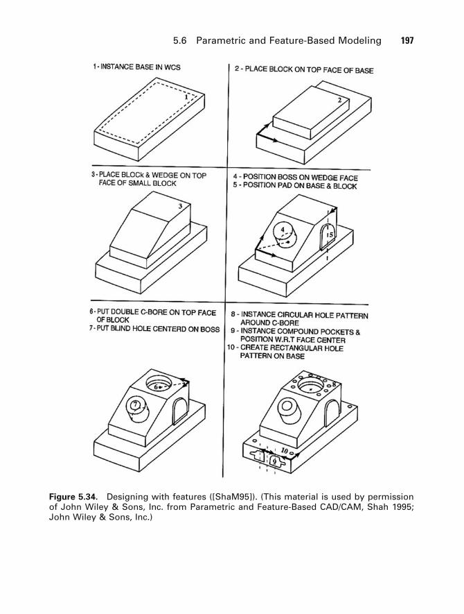
5.6 Parametric and Feature-Based Modeling 197
Figure 5.34. Designing with features ([ShaM95]). (This material is used by permissionof John Wiley & Sons, Inc. from Parametric and Feature-Based CAD/CAM, Shah 1995;John Wiley & Sons, Inc.)
GOS05 5/5/2005 6:20 PM Page 197
of the declarations is accomplished by a constraint satisfaction algorithm, an infer-ence engine, or unification, respectively. Three basic approaches are used for solvingthe constraint problem: constraint graphs where the nodes are geometric entities and the edges are the constraints, logical assertions, or algebraic equations that areexpressed symbolically and solved symbolically. None of the approaches are easy. See[LiON02] for an example of feature mapping in a design-by-feature system.
In conclusion, many modelers are now supporting features. Overall, b-rep mod-elers, in particular those that support nonmanifolds, seem better suited to the featurerecognition task than CSG modelers. The only advantage of the latter is in editing butthis can also be dealt with in a b-rep modeler. For example, consider an object withslots of varying lengths. Changing the length of the slots may cause them to intersect.With a CSG representation the history of any changes can be maintained relativelyeasily, whereas with a boundary representation such changes might cause radicalchanges in the relationships of facets. [Prat87b] mentions the following feature-specific advantages of a boundary representation:
(1) Features are usually best described in terms of faces, edges, etc.(2) Dimensioning and tolerancing of features need these low-level entities.(3) CSG representations can be ambiguous. See Figure 5.33 again.(4) Local operations for feature manipulation are available in the design stage.
Feature recognition algorithms for b-rep modelers divide into two types: those thatuse purely surface information and those that use volume decompositions. The latterseem to be a better approach but are not as developed yet.
[Prat87a] and [Prat87b] have a nice survey of work in feature based modelingfrom 1980 to 1987.
Finally, since there are a number of feature-based modelers, it is important thatone can exchange data between them. One might also want to input some feature datato an application program. STEP (Standard for exchange of product data) is a set of standards that resulted from an international effort to enable this exchange. See[ShaM95] for an overview and additional references.
5.7 Functions and Algorithms
In addition to modeling objects, modelers must also be able to perform a variety ofoperations on the objects that they have modeled. As indicated in the introduction,modeling involves modeling maps as well as objects. Here is a sample of some queriesusers may want to make and actions they may want to perform:
(1) Find physical propertie of objects: center of mass, moments of inertia, area,volume, . . .
(2) Find geometrical properties of objects: distances between objects, collisiondetection, intersections and otherBoolean set operations, . . .
(3) Perform geometrical operations: rigid motions, . . .(4) Numerical control related operations: milling, lathing, . . .
198 5 Approaches to Geometric Modeling
GOS05 5/5/2005 6:20 PM Page 198

5.8 Data Structures 199
In a modeler mathematical functions get replaced by algorithms. We want a commutative diagram as shown in Figure 5.35. Some issues that arise are:
(1) A “correct” algorithm must perform the “correct” action on all valid inputs.This is a serious issue in the context of computers because of round-off errors.For example, finding the intersection of two rectangles should work if theyonly touch along a face.
(2) If an input to an algorithm is meaningless or invalid the algorithm should
(a) inform the user, and(b) still return some answer which will not cause the system to crash
(3) An algorithm should be efficient. If objects have several representations itshould be smart enough to pick the best one for its task.
(4) An algorithm should be as general as possible to allow extensions.
We can see from this discussion that modelers must deal with many tasks thatfall into the field of computational geometry, which deals with finding geometric algorithms and analyzing them. In this regard we should mention the relatively newbut growing area of research into genetic algorithms. These algorithms are a class of search algorithms that are proving to be very useful in the complex optimizationproblems encountered by modelers. An overview of this topic can be found in[RenE03].
5.8 Data Structures
5.8.1 Data Structures for Boundary Representations
Anyone interested in implementing a geometric modeling program will quickly facethe problem of choosing appropriate data structures for the geometry that is to bemodeled. As usual, one wants data structures that will be efficient in both space andexecution times of algorithms. This section will briefly look at this issue in the casewhere we use a boundary representation for linear polyhedra. The next section willlook at what one can do in the case of volume rendering.
Rendering linear polyhedra, or cell complexes in general, involves two parts: theabstract structure of the complex and the actual data. To describe the structure meansdescribing various adjacency relations between the cells of the space.
Figure 5.35. Relationship between functionsand algorithms.
GOS05 5/5/2005 6:20 PM Page 199

200 5 Approaches to Geometric Modeling
Definition. A d-dimensional cell is said to be adjacent to an e-dimensional cell if
(1) d π e and one is contained in the other,(2) d = e > 0, and they have a (d–1)-dimensional cell in common, or(3) d = e = 0, and they are the two ends of some 1-dimensional cell (edge).
In our discussion here we shall restrict ourselves to two-dimensional complexes.Algorithms dealing with such complexes typically need adjacency information suchas the set of edges of a face or the set of faces that contain a given vertex. We shalluse the following notation:
notation what it meansx Æ y x is adjacent to yx Æ Y the set of objects of type Y adjacent to x, that is,
{y | y is an object of type Y and x Æ y}X Æ Y the sets {x Æ Y | x is an object of type X}
In the context of this notation, capital letters such as X and Y will be one of the typesV (vertex), E (edge), or F (face). |X| will denote the number of objects of type X. Weshall refer to X Æ Y as an adjacency relation.
The nine possible types of adjacency information between vertices, edges, andfaces are shown in Figure 5.36. If a data structure contains one of these adjacencyrelations explicitly, then we shall say that one has direct access to that information.For example, the notation E Æ V means that each edge has direct access to both ofits vertices and V Æ V means that each vertex has direct access to all of the verticesadjacent to it. Call a relation X Æ X a self-relation.
Two questions which need to be addressed when choosing a data structure are:
(1) Does the data structure adequately describe the topology of the spaces thatare represented? If so, then we shall say that it is topologically adequate.
(2) What is the complexity of determining the truth of x Æ y or computing some x Æ Y given the adjacency relations defined explicitly by the data structure.
[Weil85] has an extensive discussion of question (1). The topologically adequate adja-cency relationships are identified and proved to be that. We shall not repeat those
Figure 5.36. Possible face-edge-vertex adjacencydata.
GOS05 5/5/2005 6:20 PM Page 200

5.8 Data Structures 201
arguments here but simply refer the interested reader to that paper. Rather, we wantto concentrate on the answer to (2) and summarize the main results of [NiBl94]. Itshould be noted however, that all the adjacency relations that we mention later on ashaving the best complexity properties are also topologically adequate.
First of all, as Ni and Bloor point out, we need to distinguish between complex-ity in the context of a particular implementation and complexity at the abstract datastructure level. [NiBl94] analyze the latter, which is implementation independent, andgive answers in terms of the number of direct accesses of information and the numberof set operations, such as union, intersection, etc., that are needed. A discussion ofthe costs involved in the context of some specific implementations, in particular, edge-based ones, can be found in [Weil85].
As an example of how one can compute the implementation independent cost ofan adjacency relation that may be needed for an algorithm, suppose that a single non-self-relation X Æ Y is given. Algorithm 5.8.1.1 computes the inverse adjacency rela-tion Y Æ X. The cost of this algorithm is |X| direct accesses, |X| set membership tests,and at most |X||Y| unions for a total of 2|X| + |X||Y| steps. Ni and Bloor analyze in asimilar way the costs of all the other possible queries for any given set of adjacencyrelations. One relation, namely, the E Æ E relation, is treated as a special case. Some-times data structures are used that do not store all objects adjacent to a given object.For historical reasons, due to the influential papers [Baum72] and [Baum75], theedge-edge adjacency relation has come to denote a more restricted relation in thatonly two of the edges adjacent to a given edge are listed.
Baumgart’s Winged Edge Representation. In this representation each face isassumed to be bounded by a set of disjoint edge cycles. One of these is the outside
An algorithm for computing Y Æ X f rom X Æ Y :
Let xi , 1 £ i £ |X| , and yj , 1 £ j £ |Y|, denote the objects of type X and Y, respectively.
for j:=1 to |Y| dobegin
Initialize a set Xj of objects of type X to empty;for i:=1 to |X| do
beginOne direct access gives us xi Æ Y; If yj Œ (xi Æ Y) then Xj = Xj » { xi };
endend;
The collection of sets Xj now constitutes Y Æ X .
Algorithm 5.8.1.1. Computing the inverse adjacency relation Y Æ X.
GOS05 5/5/2005 6:20 PM Page 201
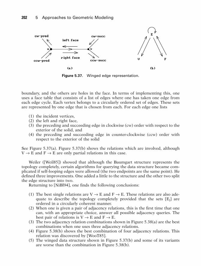
202 5 Approaches to Geometric Modeling
boundary, and the others are holes in the face. In terms of implementing this, oneuses a face table that consists of a list of edges where one has taken one edge fromeach edge cycle. Each vertex belongs to a circularly ordered set of edges. These setsare represented by one edge that is chosen from each. For each edge one lists
(1) the incident vertices,(2) the left and right face,(3) the preceding and succeeding edge in clockwise (cw) order with respect to the
exterior of the solid, and(4) the preceding and succeeding edge in counter-clockwise (ccw) order with
respect to the exterior of the solid
See Figure 5.37(a). Figure 5.37(b) shows the relations which are involved, although V Æ E and F Æ E are only partial relations in this case.
Weiler ([Weil85]) showed that although the Baumgart structure represents thetopology completely, certain algorithms for querying the data structure became com-plicated if self-looping edges were allowed (the two endpoints are the same point). Hedefined three improvements. One added a little to the structure and the other two splitthe edge structure into two.
Returning to [NiBl94], one finds the following conclusions:
(1) The best single relations are V Æ E and F Æ E. These relations are also ade-quate to describe the topology completely provided that the sets {Ej} areordered in a circularly coherent manner.
(2) When one is given a pair of adjacency relations, this is the first time that onecan, with an appropriate choice, answer all possible adjacency queries. Thebest pair of relations is V Æ E and F Æ E.
(3) The two adjacency relation combinations shown in Figure 5.38(a) are the bestcombinations when one uses three adjacency relations.
(4) Figure 5.38(b) shows the best combination of four adjacency relations. This relation was discovered by [WooT85].
(5) The winged data structure shown in Figure 5.37(b) and some of its variantsare worse than the combination in Figure 5.38(b).
Figure 5.37. Winged edge representation.
GOS05 5/5/2005 6:20 PM Page 202
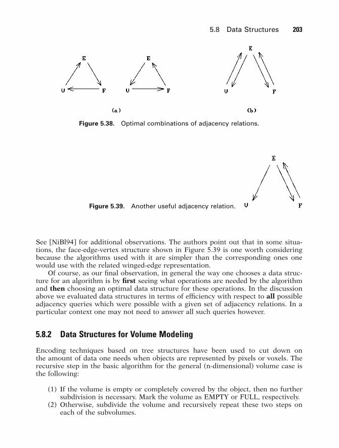
5.8 Data Structures 203
See [NiBl94] for additional observations. The authors point out that in some situa-tions, the face-edge-vertex structure shown in Figure 5.39 is one worth consideringbecause the algorithms used with it are simpler than the corresponding ones onewould use with the related winged-edge representation.
Of course, as our final observation, in general the way one chooses a data struc-ture for an algorithm is by first seeing what operations are needed by the algorithmand then choosing an optimal data structure for these operations. In the discussionabove we evaluated data structures in terms of efficiency with respect to all possibleadjacency queries which were possible with a given set of adjacency relations. In aparticular context one may not need to answer all such queries however.
5.8.2 Data Structures for Volume Modeling
Encoding techniques based on tree structures have been used to cut down on the amount of data one needs when objects are represented by pixels or voxels. Therecursive step in the basic algorithm for the general (n-dimensional) volume case isthe following:
(1) If the volume is empty or completely covered by the object, then no further subdivision is necessary. Mark the volume as EMPTY or FULL, respectively.
(2) Otherwise, subdivide the volume and recursively repeat these two steps oneach of the subvolumes.
Figure 5.38. Optimal combinations of adjacency relations.
Figure 5.39. Another useful adjacency relation.
GOS05 5/5/2005 6:20 PM Page 203

204 5 Approaches to Geometric Modeling
The binary nature of the algorithm suggests a binary tree structure, but this is not as efficient as the quadtree in the two-dimensional case and octree in the three-dimensional case.
Quadtrees. Assume that a planar region is contained in a rectangle. For example,consider the shaded region R in Figure 5.40(a). Now change the general algorithmabove to the following:
(1) If the region covers the current rectangle or is disjoint from it, then stop sub-dividing and return that fact; otherwise,
(2) divide the rectangle into four equal parts and repeat these two steps for eachof the subrectangles.
For the region R in Figure 5.40(a) we shall end up with a subdivision as indicated in the figure. The region can therefore be represented by a tree structure, called a quadtree, where each node has up to four nonempty subtrees. If we label the foursubrectangles of a rectangle as indicated in Figure 5.41(a), then the Figure 5.41(b)shows the tree structure for R.
Quadtrees can also be used to represent curved regions as shown in Figure 5.40(b)by modifying the criteria for when one quits subdividing in one of two ways:
Figure 5.40. Quadtree examples.
Figure 5.41. Quadtree structure.
GOS05 5/5/2005 6:20 PM Page 204

5.9 Converting Between Representations 205
(1) We could specify a cutoff depth below which we do not subdivide, or(2) rather than requiring that the region either misses or covers a rectangle
completely, we can quit if it “almost” misses or quits, that is, one uses thresh-olds on the percentage of area covered.
Octrees. Octrees are the three-dimensional generalization of quadtrees. In the caseof octrees we divide a cube into eight octants. See Figure 5.42. We can then encodeobjects with trees where each node has up to eight nonempty subtrees. Octrees aregenerated for objects analogous to how quadtrees are generated.
One can show that the number of nodes in a quadtree or octree are typically proportional to the size of the object’s boundary, although it is possible to create some worse cases. The intuitively obvious reason for that is that the only time oneneeds to subdivide is when a cell is crossed by the boundary.
The quadtree and octree representations for objects have many nice propertiesand they have been studied extensively in order to store and process them efficiently.Boolean set operations are relatively easy. One traverses both trees in parallel andtakes the appropriate steps at each corresponding pair of nodes. Algorithms exist forfinding a pixel or voxel or finding neighboring pixels or voxels in the tree. These areoperations that one often needs. Some simple transformations, such as rotations by90 degrees, scaling by powers of 2, and reflections are easy. Other transformations arenot. Aliasing is a big problem when performing these transformations. For moredetails see the references in the spatial data structure section of the bibliography.
5.9 Converting Between Representations
The need for algorithms that convert from one representation to another exists notonly because modelers using different representations may want to exchange geo-metric data but especially because modelers increasingly seem to maintain multiplerepresentations internally. By in large, the problem seems to have only been dealt within an ad hoc way. We begin by addressing the two classical CSG-to-b-rep and b-rep-to-CSG problems. We end with some comments about the IGES data exchange standard between modelers.
The CSG-to-b-rep problem is the boundary evaluation problem in CSG that wasfirst studied systematically in [ReqV85]. An early algorithm for polyhedral objects can
Figure 5.42. Octree subdivision.
GOS05 5/5/2005 6:20 PM Page 205
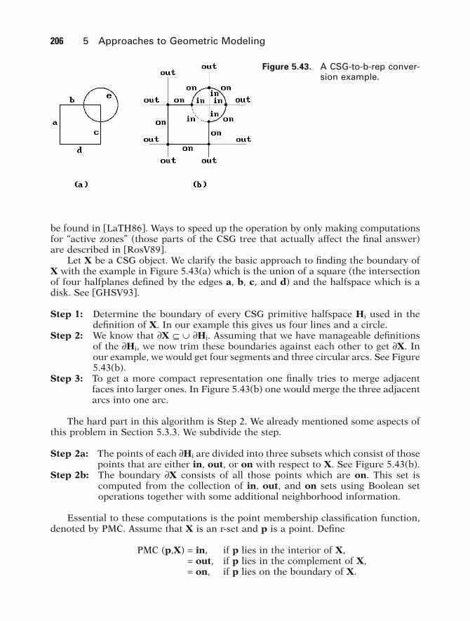
206 5 Approaches to Geometric Modeling
be found in [LaTH86]. Ways to speed up the operation by only making computationsfor “active zones” (those parts of the CSG tree that actually affect the final answer)are described in [RosV89].
Let X be a CSG object. We clarify the basic approach to finding the boundary ofX with the example in Figure 5.43(a) which is the union of a square (the intersectionof four halfplanes defined by the edges a, b, c, and d) and the halfspace which is adisk. See [GHSV93].
Step 1: Determine the boundary of every CSG primitive halfspace Hi used in thedefinition of X. In our example this gives us four lines and a circle.
Step 2: We know that ∂X Õ » ∂Hi. Assuming that we have manageable definitionsof the ∂Hi, we now trim these boundaries against each other to get ∂X. Inour example, we would get four segments and three circular arcs. See Figure5.43(b).
Step 3: To get a more compact representation one finally tries to merge adjacentfaces into larger ones. In Figure 5.43(b) one would merge the three adjacentarcs into one arc.
The hard part in this algorithm is Step 2. We already mentioned some aspects ofthis problem in Section 5.3.3. We subdivide the step.
Step 2a: The points of each ∂Hi are divided into three subsets which consist of thosepoints that are either in, out, or on with respect to X. See Figure 5.43(b).
Step 2b: The boundary ∂X consists of all those points which are on. This set is computed from the collection of in, out, and on sets using Boolean setoperations together with some additional neighborhood information.
Essential to these computations is the point membership classification function,denoted by PMC. Assume that X is an r-set and p is a point. Define
PMC (p,X) = in, if p lies in the interior of X,= out, if p lies in the complement of X,= on, if p lies on the boundary of X.
Figure 5.43. A CSG-to-b-rep conver-sion example.
GOS05 5/5/2005 6:20 PM Page 206
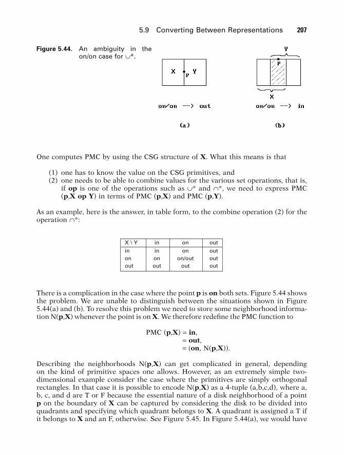
5.9 Converting Between Representations 207
One computes PMC by using the CSG structure of X. What this means is that
(1) one has to know the value on the CSG primitives, and(2) one needs to be able to combine values for the various set operations, that is,
if op is one of the operations such as »* and «*, we need to express PMC(p,X op Y) in terms of PMC (p,X) and PMC (p,Y).
As an example, here is the answer, in table form, to the combine operation (2) for theoperation «*:
Figure 5.44. An ambiguity in theon/on case for »*.
X \ Y in on out
in in on outon on on/out outout out out out
There is a complication in the case where the point p is on both sets. Figure 5.44 showsthe problem. We are unable to distinguish between the situations shown in Figure5.44(a) and (b). To resolve this problem we need to store some neighborhood informa-tion N(p,X) whenever the point is on X. We therefore redefine the PMC function to
PMC (p,X) = in,= out,= (on, N(p,X)).
Describing the neighborhoods N(p,X) can get complicated in general, depending on the kind of primitive spaces one allows. However, as an extremely simple two-dimensional example consider the case where the primitives are simply orthogonalrectangles. In that case it is possible to encode N(p,X) as a 4-tuple (a,b,c,d), where a,b, c, and d are T or F because the essential nature of a disk neighborhood of a pointp on the boundary of X can be captured by considering the disk to be divided intoquadrants and specifying which quadrant belongs to X. A quadrant is assigned a T ifit belongs to X and an F, otherwise. See Figure 5.45. In Figure 5.44(a), we would have
GOS05 5/5/2005 6:20 PM Page 207

208 5 Approaches to Geometric Modeling
N(p,X) = (F,F,T,T) and N(p,Y) = (T,T,F,F). In Figure 5.44(b), N(p,X) = (F,F,T,T) and N(p,Y) = (F,F,T,T). Simple Boolean operations on these representations wouldthen determine the neighborhood of points in the on/on case. In a correspondingthree-dimensional example of orthogonal blocks one would use an encoding based onoctants. The reader is referred to [Tilo80] and [ReqV85] for a discussion of how onewould handle more general cases.
Next, we consider the problem of converting from a b-rep to CSG, which is muchmore difficult than going in the opposite direction. The basic idea is to use the half-spaces associated to the faces of the b-rep to describe a CSG representation. Unfor-tunately, this may not work as the example in Figure 5.46(a) shows. The shaded regionconsisting of the three regions A, B, and C is our solid X and H1 and H2, the interi-ors of the horizontal and vertical ellipse, respectively, are the halfspaces associated tothe faces of X. No CSG representation which only uses these two halfspaces will rep-resent X because any space defined by such a representation that contains region Cwill also contain region D. We have to introduce some additional halfspaces, calledseparating planes. The separating plane and the halfplane H3 below it shown in Figure5.46(b) will do the job for the space X. For example,
(5.5)X H H H H H H= «( ) » «( ) » «( )3 1 3 2 1 2* * * * * .
Figure 5.45. Neighborhood classificationof an on/on point.
Figure 5.46. The need for separating planes.
GOS05 5/5/2005 6:20 PM Page 208

Therefore, before continuing, we need to answer the question: When can a spacebe described in terms of unions, intersections, and complements of halfspaces?Assume that we have a finite collection of halfspaces H = {H+(f1), H+(f2), . . . , H+(fk)}.Although there is an infinite number of ways that these spaces can be combined withthe regular operators »*, «*, or -*, the following is true:
5.9.1 Theorem. All possible combinations of the halfspaces in H using the opera-tors »*, «*, or -* will generate only a finite number of regular spaces X and each ofthese can be represented by a unique expression in the form
(5.6)
and each hj is either H+(fj) or H-(fj).
Proof. See [ShaV93].
As an example of this theorem, consider the space X in Figure 5.46(b) again. Theunique decomposition of X guaranteed by the theorem is the one below:
(5.7)
(The decomposition in equation (5.5) does not have the right structure.)In general, let us call any space like Pi in equations (5.6) a canonical intersection
term for the collection of halfspaces H. Note that the interior of every canonical inter-section term is the intersection of the interior of the halfspaces that defined thatcanonical intersection. This leads to the main theorem about when a space admits aCSG representation based on a given set of halfspaces.
5.9.2 Theorem. Let H = {H1, H2, . . . , Hk} be a collection of halfspaces. A solid Xwith the property that ∂X Ã (∂H1 » ∂H2 » . . . » ∂Hk) admits a CSG representationbased on H if and only if the interior of every canonical intersection term based onH is either entirely contained in X or entirely outside of X.
Proof. See [ShaV91a].
Theorem 5.9.2 explains why the two halfspaces in Figure 5.46(a) were inadequateto describe the space X: the canonical intersection H1 «* c*(H2) is half in X and halfoutside of X.
We clarify our discussion with another example. We desire a b-rep-to-CSG conversion for the solid X in Figure 5.47(a) ([GHSV93]). The b-rep of our solid Xspecifies five halfspaces associated to each face in the boundary: four halfplanes andone disk. Figure 5.47(b) shows the in/out classification of the canonical intersectionsfor our halfspaces. We see that the regions A and B in the figure that belong to thesame canonical intersection have a different in/out classification. They are both in thesquare and outside the disk, but one is inside our solid and the other is outside it. ByTheorem 5.9.2 this means that X cannot be obtained from the given halfplanes and
X H H H H H H
H H H H H H
= « «( ) » « « ( )( ) »« « ( )( ) » « « ( )( )
3 1 2 3 1 2
3 2 1 1 2 2
* * * * * * *
* * * * * * * .
c
c c
X h h h= = « « «U Ki
i i kwhere* , * * *P P 1 2
5.9 Converting Between Representations 209
GOS05 5/5/2005 6:20 PM Page 209
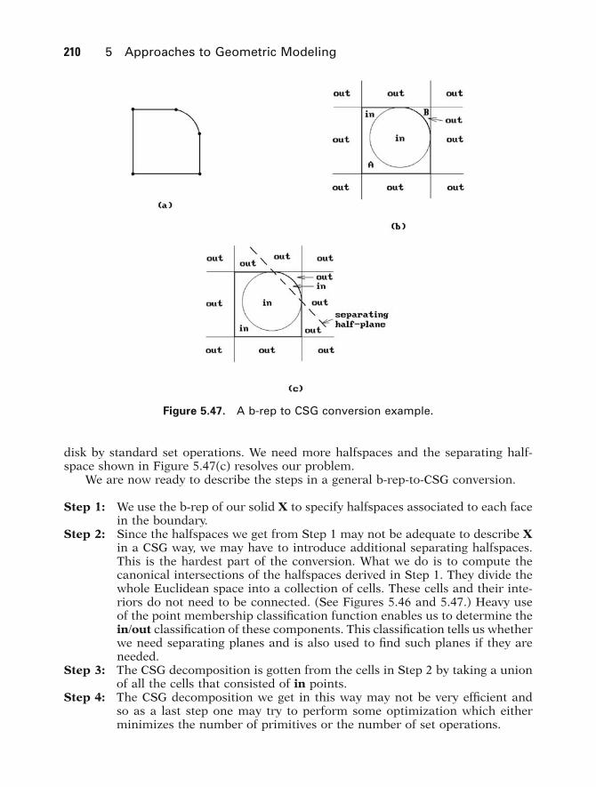
210 5 Approaches to Geometric Modeling
disk by standard set operations. We need more halfspaces and the separating half-space shown in Figure 5.47(c) resolves our problem.
We are now ready to describe the steps in a general b-rep-to-CSG conversion.
Step 1: We use the b-rep of our solid X to specify halfspaces associated to each facein the boundary.
Step 2: Since the halfspaces we get from Step 1 may not be adequate to describe Xin a CSG way, we may have to introduce additional separating halfspaces.This is the hardest part of the conversion. What we do is to compute thecanonical intersections of the halfspaces derived in Step 1. They divide thewhole Euclidean space into a collection of cells. These cells and their inte-riors do not need to be connected. (See Figures 5.46 and 5.47.) Heavy useof the point membership classification function enables us to determine thein/out classification of these components. This classification tells us whetherwe need separating planes and is also used to find such planes if they areneeded.
Step 3: The CSG decomposition is gotten from the cells in Step 2 by taking a unionof all the cells that consisted of in points.
Step 4: The CSG decomposition we get in this way may not be very efficient and so as a last step one may try to perform some optimization which eitherminimizes the number of primitives or the number of set operations.
Figure 5.47. A b-rep to CSG conversion example.
GOS05 5/5/2005 6:20 PM Page 210

For more details see [ShaV91a], [ShaV91b], and [ShaV93]. [GHSV93] has a niceoverview of the generic representation conversion process and the general principlesthat are involved. Step 4 above points to one of the stumbling blocks to having a nicetheory of conversions between different representations. The answer may not be well-defined. In the b-rep-to-CSG case, we do not have a clear idea of which of the manypossible primitives that one can use are best.
As we have seen, converting between different representations is potentially a hardproblem. There is another related problem. Two modelers may use basically the samerepresentation scheme but have implemented them differently. This is hardly sur-prising since each had a different team of programmers. What we have here is animplementation conversion problem. Because there are many commercial modelingsystems in use, this is a real problem since many businesses are not able to assumethat all needed data will be generated internally and there is a need to transfer data from one system to another. IGES (Initial Graphics Exchange Specification)was developed to solve this problem and enable different systems to exchange databetween themselves. To use IGES, a modeling system must have translators thatconvert from their representations to those of IGES and vice versa. A person wishingto transfer data from system A to system B would then first use system A’s IGES trans-lator to translate the system A data into the IGES format and write this to a file. Thatfile would then be read by system B’s IGES translator that would convert the IGESdata into system B’s own internal format.
IGES is not perfect and it is easy to complain about its constraints. There isanother more advanced data exchange format STEP that allows for much more high-level descriptions than the relatively simple annotated geometry formats ofIGES, but we refer the reader to [ShaM95] for that. Nice features of a modeling systemcan get lost in the translation to and from IGES. A direct translation from one system’sdata structure into the other’s would usually be more efficient. The latter approachwould therefore be the way to go in certain dedicated situations. However, it is certainly much simpler to write one translator (for IGES) than writing many (one for each external modeling system). Writing translators is a nontrivial task. Further-more, modeling systems continue to evolve and one would have to keep updating any direct translators. IGES also continues to change with the times, but at least onlyone update has to be written if one uses it. The bottom line is that IGES is a cost-effective solution to the geometric data transfer problem that works. See Appendix Cfor a summary of how various object types are represented by IGES and the formatof an IGES file.
5.10 Round-off Error and Robustness Issues
Accuracy and robustness are important issues in numerical computations. For anoverview of some common pitfalls see [McCa98]. Because geometric modelinginvolves a great many numerical algorithms, one wants to minimize the potential ofround-off errors and avoid situations where small changes can lead to radically dif-ferent results. To accomplish this one must choose carefully between different algo-rithms and representations for objects. In this section we only scratch the surface of
5.10 Round-off Error and Robustness Issues 211
GOS05 5/5/2005 6:20 PM Page 211

212 5 Approaches to Geometric Modeling
this difficult subject. Currently, solutions to numerical problems tend to be targetedto specific areas. What are still needed are general solutions. In the meantime it islargely up to users to be aware of potential problems and to take steps on their ownto try to avoid them.
One of the first things one learns about real numbers when programming is thatone almost never tests for equality but rather asks whether numbers are close enough.Modeling systems tend to use plenty of epsilons, small positive constants that are usedto define when quantities are supposed to be considered equal. Getting correct yes/noanswers when one only has approximations is not easy. So often the mathematicalanswer to a geometric problem is short and simple, but the computer program thatimplements it is much longer and messy. For example, to determine whether a pointin the plane lies on a line is trivial mathematically. One can simply check whether thepoint satisfies the equation of the line, which involves checking whether some expres-sion equals zero. In a computer program, testing for zero would probably be toostrong a test and one would be satisfied if the expression is suitably small. This mightnot cause any problems by itself, but errors can propagate. Treating two lines as par-allel if they are only almost parallel might be all right, but if a sequence of lines arealmost parallel, then the first and the last might be quite far from being parallel. Fur-thermore, no matter how small the epsilons, there is a potential of getting inconsis-tencies in the geometric database. In Figure 5.48, if the segment AB is close to beingparallel to the top face f of the solid, then in the process of intersecting it with thesolid, one may conclude that AB intersects the face f in the segment CD. On the otherhand, one may get a more accurate intersection with the side face g and conclude inthat case that the line does not intersect CD. This might leave an incorrect descrip-tion of AB in the database as a composition of three segments. The author has per-sonally known of commercial CAD systems that (at least in their initial version) wouldcrash in some constructions that involved solids that touched each other along essen-tially parallel faces.
Maintaining the orthogonality of orthogonal matrices is another problem in com-puter graphics. Orthogonal matrices may become nonorthogonal after numeroustransformations. This is a serious problem in robotics where moving joints meanstransforming matrices. What one needs to do here is to maintain a count of thenumber of transformations that have been performed and then periodically reorthog-onalize the matrices. Of course, since one does not know which values are incorrect,the new matrices, although orthogonal, are probably not what they should be mathematically.
Figure 5.48. Intersection inconsistencies due toround-off errors.
GOS05 5/5/2005 6:20 PM Page 212

Numerical analysis is clearly the first place to look for answers about accuracy ina world of approximations. A lot is known about the accuracy of the output of a com-putation given the accuracy of the input. For example, to get precise answers withlinear problems one would have to perform computations using four to five times theprecision of the initial data. In the case of quadratic problems, one would need fortyto fifty times the precision. Sometimes there may be guidelines that help one improvethe accuracy of results. Given the problems with floating point arithmetic, one couldtry other types of arithmetic.
Bounded Rational Arithmetic. This is suggested in [Hoff89] and refers to restrict-ing numbers to being rational numbers with denominators that are bounded by agiven fixed integer. One can use the method of continued fractions to find the bestapproximation to a real by such rationals.
Infinite Precision Arithmetic. Of course, there are substantial costs involved inthis.
“Exact” Arithmetic. This does not mean the same thing as infinite precision arithmetic. The approach is described in [Fort95]. The idea is to have a fixed but rel-atively small upper bound on the bit-length of arithmetic operations needed tocompute geometric predicates. This means that one can do integer arithmetic.Although one does not get “exact” answers, they are reliable. It is claimed that bound-ary-based faceted modelers supporting regularized set operators can be implementedwith minimal overhead (compared with floating point arithmetic). Exact arithmeticworks well for linear objects but has problems with smooth ones. See also [Yu92] and[CuKM99].
Interval Analysis. See Chapter 18 for a discussion of this and also [HuPY96a] and[HuPY96b].
Just knowing the accuracy is not always enough if it is worse than one would like. Geometric computations often involve many steps. Rather than worrying aboutaccuracy only after data structures and algorithms have been chosen, one shouldperhaps also use accuracy as one criterion for choosing the data structures and algorithms.
One cause for the problem indicated in Figure 5.48 is that one often uses differ-ent computations to establish a common fact. The question of whether the linesegment intersected the edge of the cube was answered twice – first by using the facef and second by using the face g. The problem is in the redundancy in the represen-tation of the edge and the fact that the intersection is determined from a collectionof isolated computations. If one could represent geometry in a nonredundant way,then one would be able to eliminate quite a few inconsistency problems. Furthermore,the problem shown in Figure 5.48 would be resolved if, after one found the intersec-tion with face f, one would check for intersections with all the faces adjacent to f andthen resolve any inconsistencies.
We give a brief overview of an approach to achieving robust set operations onlinear polyhedra described in [HoHK89] and [Hoff89]. It involves both data structures
5.10 Round-off Error and Robustness Issues 213
GOS05 5/5/2005 6:20 PM Page 213
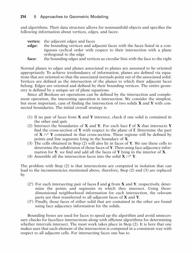
and algorithms. Their data structure allows for nonmanifold objects and specifies thefollowing information about vertices, edges, and faces:
vertex: the adjacent edges and facesedge: the bounding vertices and adjacent faces with the faces listed in a con-
tiguous cyclical order with respect to their intersection with a planeorthogonal to the edge
face: the bounding edges and vertices as circular lists with the face to the right
Normal planes to edges and planes associated to planes are assumed to be orientedappropriately. To achieve irredundancy of information, planes are defined via equa-tions that are oriented so that the associated normals point out of the associated solid.Vertices are defined as the intersection of the planes to which their adjacent facesbelong. Edges are oriented and defined by their bounding vertices. The entire geom-etry is defined by a unique set of plane equations.
Since all Boolean set operations can be defined by the intersection and comple-ment operation, the interesting operation is intersection. We consider the simplest,but most important, case of finding the intersection of two solids X and Y with con-nected boundaries. The initial overall strategy is
(1) If no pair of faces from X and Y intersect, check if one solid is contained inthe other and quit.
(2) Intersect the boundaries of X and Y. For each face f of X that intersects Yfind the cross-section of Y with respect to the plane of f. Determine the partof X «* Y contained in that cross-section. These regions will be defined bypoints and line segments lying in the boundary of X.
(3) The cells obtained in Step (2) will also lie in faces of Y. We use these cells todetermine the subdivision of those faces of Y. Then using face adjacency infor-mation for Y, we find and add all the faces of Y lying in the interior of X.
(4) Assemble all the intersection faces into the solid X «* Y.
The problem with Step (2) is that intersections are computed in isolation that canlead to the inconsistencies mentioned above, therefore, Step (2) and (3) are replacedby
(2¢) For each intersecting pair of faces f and g from X and Y, respectively, deter-mine the points and segments in which they intersect. Using three-dimensional neighborhood information for each intersection, the relevantparts are then transferred to all adjacent faces of X and Y.
(3¢) Finally, those faces of either solid that are contained in the other are foundusing face adjacency information for the solids.
Bounding boxes are used for faces to speed up the algorithm and avoid unneces-sary checks for face/face intersections along with efficient algorithms for determiningwhether intervals intersect. The most work takes place in Step (2). It is here that onemakes sure that each element of the intersection is computed in a consistent way withrespect to all adjacent cells. For intersecting faces one has to
214 5 Approaches to Geometric Modeling
GOS05 5/5/2005 6:20 PM Page 214

(1) find and analyze the points and segments in the intersection,(2) transfer the results to adjacent faces in X and Y, and(3) link the various intersection pieces into complete face and edge descriptions.
These steps involve careful analysis of neighborhoods of cells. The six major casesarise from face/face, face/edge, face/vertex, edge/edge, edge/vertex, and vertex/vertexintersections.
The authors of [HoHK89] reported that when the algorithm we just described wasimplemented, very substantial improvements in robustness were realized comparedwith other modelers. Their test cases included such typically difficult cases as findingthe intersection of two cubes, where the second is a slightly rotated version of thefirst. We refer the reader to that paper and [Hoff89] for additional ideas about dealingwith accuracy and robustness that we do not have space to get into here. More paperson robustness can be found in [LinM96]. See also [DeSB92] and [EdaL99]. Often theproblems we have talked about are caused by the fact that they are special cases orsome sort of degeneracy. There is no problem determining whether two lines inter-sect if they are reasonably skew. Therefore, perhaps one can always arrange it so thatthey are or that objects are not almost touching, etc., by perturbing them slightly. Thisis the basis for an approach to robustness described in [EdeM90]. Objects are put intogeneral position by a small perturbation; however, the perturbation is done symboli-cally. Nothing is actually ever perturbed.
Finally, because conics are such an important class of spaces in modeling, wefinish this section with some facts about the robustness of some of their standard rep-resentations. Four common ways to define conic curves are:
(1) via the general quadratic equation(2) in standard form at the origin along with a transformation(3) via a few points and/or reals (For example, one can define an ellipse in terms
of its center, major axis, and major and minor axes lengths.)(4) via projective geometry type constructions
Which is best? It is well known that (1) is by far the worst representation. Changingcoefficients even just slightly, can, in certain circumstances, lead to incorrect conclu-sions as to the type of the conic. According to [Wils87], (2) and (3) are the best with(3) slightly better.
5.11 Algorithmic Modeling
Sections 5.3.1–5.3.9 discussed various specific approaches to geometric modeling.This section takes a more global view and tries to identify some unifying principlesbehind some of the details. Specifically, the relatively recent generative modelingscheme and the natural phenomena and physically based modeling schemes are exam-ples of what is referred to as algorithmic or procedural modeling in [GHSV93]. Algo-rithmic modeling refers to that part of geometric modeling where one uses algorithmsto define and manipulate objects or functions rather than nonconstructive definitions.
5.11 Algorithmic Modeling 215
GOS05 5/5/2005 6:20 PM Page 215

Sometimes one has a choice, but even though the spaces we might get can bedescribed by a function that parameterizes the space or defines it implicitly, there arereasons for why it might be useful to generate a space algorithmically:
(1) Not all spaces can be computed and sometimes, like in the case of fractals,one can only describe them by a limiting process.
(2) The geometry of a space sometimes changes over time or due to external influ-ences and the best way to describe this may be algorithmically.
(3) Some complex geometric structures are too complicated to describe by functions.
(4) Algorithmic descriptions may give rise to added flexibility and power.
In [GHSV93] algorithmic models are divided into four main classes.
Geometry-based models: Generative modeling is an example. Its models are parameterized by properties and transformations
Functional-based models: These models are defined by functions and modified byother functions. Texture functions are an example howfunctions can modify geometry.
Grammar-based models: Here the structure is defined by a language and agrammar for that language. The grammars can bedivided into geometric (fractals and their initiator/generator paradigm) and topological (graftals) grammars.
Physics-based models: The models are controlled by the laws of physics. SeeSection 5.5. Also included here are particle systems,deformable models (elastic/inelastic), and constraintsystems.
For more details see [GHSV93].Looked at abstractly, what the theory of algorithmic modeling adds to “standard”
geometric modeling is a symbol generation mechanism that can be either determin-istic or probabilistic. To formalize this we must generalize the notion of a Turingmachine to one that can deal with continuous functions.
Although the theory of computation is a well-developed subject, the classicaltheory of Turing machines deals with discrete computations. Here, an analysis of thecomplexity of a computation takes into account the size of numbers in terms of the number of bits in their binary representation. On the other hand, when we dealwith continuous geometry, as we do in geometric modeling, it would be nice to make our baseline the reals and to consider the cost of basic arithmetic operations,such as multiplication, independent of their “size.” To put it another way, since geometric shapes are usually defined by parameterizations or implicitly, we would liketo have a concept of computability based on reals and appropriate “computable” con-tinuous functions. We would then like to ask the same types of questions as in thediscrete Turing machine case. For example, which topological spaces are “com-putable” in this setting? In recent years, such a continuous theory of computation has
216 5 Approaches to Geometric Modeling
GOS05 5/5/2005 6:20 PM Page 216

5.11 Algorithmic Modeling 217
been developed that formalizes the notion of a machine over the reals. See [BlSS89]or [GHSV93]. We would like to mention a few of the highlights of the theory in thissection.
We motivate our definition of a machine over the reals with two examples from[BlSS89].
5.11.1 Example. Let g :C Æ C be a complex polynomial map. Since the highestorder term of g dominates, one can show that there exists a positive constant Cg sothat |z| > Cg implies that |gk(z)| Æ • as k goes to infinity. Figure 5.49 shows a flow-chart for an algorithm based on g. Right now we prefer to think of it as a state diagramfor a machine M. Clearly, M will halt precisely on those inputs z for which |gk(z)| Æ• as k goes to infinity.
5.11.2 Example. Figure 5.50 shows an algorithm that computes the greatestinteger Îx˚ for x Œ R, x ≥ 0. We again shall think of it as a state diagram of a machinethat operates on a pair (k,x). To find the greatest integer in x, one inputs (0,x).
Figure 5.49. State diagram for Example5.11.1.
Figure 5.50. Computing the greatestinteger in x.
GOS05 5/5/2005 6:20 PM Page 217

What is notable about the two examples here is the state diagram of the“machines” that carried out the associated algorithms. This is what we want to gen-eralize now.
Let R be an ordered commutative ring with unity. Because there is no space to gointo lots of details, the definitions we give here will not be as general as they could bebut are aimed at the special cases R = Z or R.
Definition. A machine M over R consists of three sets I = Rm (the input space), O =Rn (the output space), and S = Rk (the state space), along with a finite connecteddirected graph G whose nodes are one of four types:
Input node: There is only one node of this type and it will be denoted by 1.It has no incoming edge and only one outgoing edge to a nodedenoted by b(1) and called the next node. Associated to this nodeis a linear injective map i : I Æ S. One thinks of i as just takingthe input and “putting it into the machine.”
Output node: These nodes have no outgoing edges. Associated to each suchnode o, there is a linear map go :S Æ O.
Computation node: Each such node c has a unique outgoing edge to a node denotedby b(c) and called the next node. Associated to the node is a poly-nomial map gc :S Æ S. If R is a field, then we can let gc be arational function.
Branch node: Each such node b has precisely two outgoing edges to nodesdenoted by b-(b) and b+(b) called next nodes. Associated to b isa polynomial hb :S Æ R, such that b+ (b) and b- (b) are associ-ated to the conditions hb(x) ≥ 0 and hb(x) < 0, respectively.
By expressing the definition of a machine over a ring graphically, it is not as com-plicated as it may sound. It leads to state diagrams just like in the Turing machinecase. The two examples above are, in fact, special cases of a machine M over the reals.In Example 5.11.1, we identify the complex numbers C with R2. The input, output,and state spaces of M are all R2. The function i associated to the input node is theidentity map and the function at the branch node is h(z) = |z|2 - Cg. In Example 5.11.2,the input, output, and state spaces are R, R, and R2, respectively. The function asso-ciated to the input node is the function from R to R2 that maps x to (0,x). At com-putation nodes, the associated function is (x,y) Æ (x + 1,y - 1). The output functionis the map from R2 to R that maps (x,y) to y.
Now, given a machine M over a ring R with nodes N, define a partial map
by G (n,s) = (n¢,s¢) where
(1) G is not defined if n is an input or output node.(2) If n is a computation node, then n¢ = b(n) and s¢ = gn(s).(3) If n is a branch node, then s¢ = s and n¢ = b+(n) if hn(s) ≥ 0 and n¢ = b-(n) if
hn(s) < 0.
G N S N S: ¥ Æ ¥
218 5 Approaches to Geometric Modeling
GOS05 5/5/2005 6:20 PM Page 218

5.11 Algorithmic Modeling 219
If we allowed rational functions in (2), then gn may not be defined because its denom-inator vanishes on s. It turns out that it is easy to overcome this technical problemand so there is no loss in generality if we assume that gn is always defined on anyvalue where we want to evaluate it.
Definition. A computation of length t is a sequence
(5.8)
where x is an element of I. The set
is called the halting set of M. The input-output map
is defined as follows: Let x ΠWM and let (5.8) be the computation with o = nt ΠO.Then
Definition. A map f :A Õ Rm Æ Rn is said to be computable over R if there exists amachine M over R so that WM = A and jM = f. In this case we say that M computes f.
Definition. A set A Õ Rm is recursively enumerable over R if A = WM for some machineM over R. It is decidable if it and its complement are both recursively enumerable overR; otherwise it is said to be undecidable.
One can show that decidability of a set A is equivalent to its characteristic func-tion being computable. Lots of interesting results about machines over a ring areproved in [BlSS89]. The ones most interesting for us here will now be mentioned.
5.11.3 Theorem. A recursively enumerable set over R is the countable union ofsemialgebraic sets.
Proof. See [BlSS89].
5.11.4 Corollary. The halting set of a machine over R is the countable union ofdisjoint semialgebraic sets. The input-output map for the machine is a piecewise poly-nomial map.
Since one can show that the Hausdorff-Besicovitch dimension of a semialgebraicset is an integer, we also get
5.11.5 Corollary. The halting set of a machine over R has integral Hausdorffdimension.
jM o tx g s( ) = ( ).
jM M O: W Æ
WM x I there= Π( ){ } is a computation of the form 5.8 with n an output nodet
1 1 1 11 1 2 22, , , , , , , , , , , ,i i i ix n s G x n s G x n s G xt t
t( )( ) ( ) = ( )( ) ( ) = ( )( ) ( ) = ( )( )K
GOS05 5/5/2005 6:20 PM Page 219

220 5 Approaches to Geometric Modeling
Corollary 5.11.4 indicates why it is reasonable to stay with semialgebraic sets intraditional geometric modeling. Corollary 5.11.5, on the other hand, shows that wedo not get fractals in this way. The next result tells us something about the sets oneencounters when trying to define fractals.
5.11.6 Theorem. The basis of attraction of a complex rational function g :C Æ C(which means the union of the basin of attraction of all attractive periodic points) isa recursively enumerable set over R. In particular, it is the countable union of semi-algebraic sets.
Proof. See [BlSS89]. It can be shown that g has only a finite number of attractiveperiodic points and that there is a polynomial h so that a point is in the basin of g ifand only if h(z) < 0 for some z in its orbit. The theorem is proved using this h and amachine very similar to the one in Example 5.11.1.
Not all basins of attraction are decidable. In fact, it is shown in [BlSS89] that theJulia set and most of its analogs are not recursively enumerable. On the other hand,one can compute semialgebraic set approximations to Julia sets.
5.12 Conclusions
In the 1970s and 1980s most modelers were based on either the boundary or CSGrepresentations or both. Here is a summary of the differences between these two rep-resentations. Roughly speaking, the advantages of the boundary representation aredisadvantages for the CSG representation and vice versa.
Advantages of b-reps: (1) It is good for efficient rendering algorithms.(2) It can handle general “free-form” or “sculptured” sur-
faces, that is, “curved” surfaces that typically aredefined implicitly or via parameterizations.
(3) It is good for local modification of models.
Disadvantages of b-reps: (1) It takes a lot of data structures and space to defineobjects.
(2) Object definitions tend to be complicated.(3) Verification of validity is difficult.
Advantages of CSG: (1) It is very compact.(2) It is a natural way to define many objects and
“perfect” for most mechanical engineering parts.(3) Validity checking is “built in.”
Disadvantages of CSG: (1) It is not good for rendering because one needs a sep-arate boundary evaluation algorithm.
(2) It may not be easy to define the motions that placeobjects in position for the Boolean set operations.
(3) It is impractical to use for sculptured surfaces orsolids bounded by such surfaces except in the most
GOS05 5/5/2005 6:20 PM Page 220

trivial cases. With the typical set of primitives, thebest that one could do for such objects, as forexample an airplane wing, is get a very inefficientapproximation.
(4) The definition of what is a “face” is more complicated.
Some modelers were hybrid systems that used the best features of boundary andCSG representations. In fact, the user interfaces for modelers are reasonably standardand hide the actual representation that is used. It is like with a database programwhere the user usually does not really know (or care) whether it is truly relational ornot. The only way one might get an inkling of the representation on which a modeleris based is by the speed and ease of completing certain queries. For example, bound-ary representations have an easier time with queries that deal with faces. A hybridsystem does have problems however:
(1) It must be able to convert between the different representation and the b-rep-to-CSG conversion is very hard.
(2) It must maintain consistency between representations. This limits its cover-age. For example, if a b-rep object came from a CSG representation and onemodifies it using a parametric surface for blending, the original CSG struc-ture can probably not be kept consistent with it. See [ShaV95].
Initially, the typical operators in b-rep modelers were the set operations basic toCSG, but gradually more and more operations were introduced into modelers, oper-ations, such as local blending operations, that were not easy to implement in a CSGmodeler. This has caused pure CSG modelers to disappear, probably also because ofthe many advantages to using spline surfaces, especially NURBS surfaces, and the factthat there is no general b-rep-to-CSG algorithm. The result is that most modelers arenow b-rep based. Volume-based modelers will also probably become more prevalentin the future with faster computers and large amounts of memory. Nevertheless, CSGhas had a fundamental impact on the way that one views geometric modeling. CSGcan be viewed as an abstract description of objects and so, whether or not a modeleris based on it, the user interfaces will continue to support it. It should be pointed outthat the parametric modeling systems that developed did not entirely avoid the prob-lems found in the dual b-rep/csg-rep systems. When a slot in the middle of a block ismoved to the edge of the block, it and the associated blend will disappear. Shapiroand Vossler ([ShaV95]) argue that such difficulties are caused by the fact that theconcept “parametric family” is not well-defined. A designer may not be able to predictwhether certain parameterizations will remain valid throughout the design process.A lot more work needs to be done in this area if one wants a design process that doesnot require human intervention in the parametric structure of an object.
A modeler’s ability to edit a model is extremely important to a user. Finding a goodway to do this is the basis of a lot of current research. We briefly discussed the medialaxis representation. Another approach called Erep is described in [GHSV93]. Its goalis to be an editable, high-level textual representation for feature based solid model-ing. It is a representation that is independent of the underlying modeler.
5.12 Conclusions 221
GOS05 5/5/2005 6:20 PM Page 221
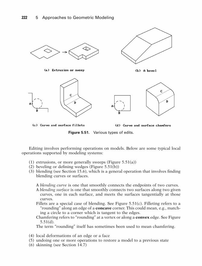
222 5 Approaches to Geometric Modeling
Editing involves performing operations on models. Below are some typical localoperations supported by modeling systems:
(1) extrusions, or more generally sweeps (Figure 5.51(a))(2) beveling or defining wedges (Figure 5.51(b))(3) blending (see Section 15.6), which is a general operation that involves finding
blending curves or surfaces.
A blending curve is one that smoothly connects the endpoints of two curves.A blending surface is one that smoothly connects two surfaces along two given
curves, one in each surface, and meets the surfaces tangentially at thosecurves.
Fillets are a special case of blending. See Figure 5.51(c). Filleting refers to a“rounding” along an edge of a concave corner. This could mean, e.g., match-ing a circle to a corner which is tangent to the edges.
Chamfering refers to “rounding” at a vertex or along a convex edge. See Figure5.51(d).
The term “rounding” itself has sometimes been used to mean chamfering.
(4) local deformations of an edge or a face(5) undoing one or more operations to restore a model to a previous state(6) skinning (see Section 14.7)
Figure 5.51. Various types of edits.
GOS05 5/5/2005 6:20 PM Page 222
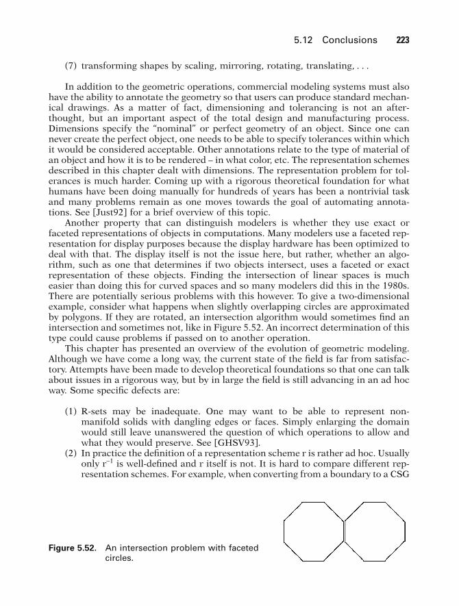
5.12 Conclusions 223
(7) transforming shapes by scaling, mirroring, rotating, translating, . . .
In addition to the geometric operations, commercial modeling systems must alsohave the ability to annotate the geometry so that users can produce standard mechan-ical drawings. As a matter of fact, dimensioning and tolerancing is not an after-thought, but an important aspect of the total design and manufacturing process.Dimensions specify the “nominal” or perfect geometry of an object. Since one cannever create the perfect object, one needs to be able to specify tolerances within whichit would be considered acceptable. Other annotations relate to the type of material ofan object and how it is to be rendered – in what color, etc. The representation schemesdescribed in this chapter dealt with dimensions. The representation problem for tol-erances is much harder. Coming up with a rigorous theoretical foundation for whathumans have been doing manually for hundreds of years has been a nontrivial taskand many problems remain as one moves towards the goal of automating annota-tions. See [Just92] for a brief overview of this topic.
Another property that can distinguish modelers is whether they use exact orfaceted representations of objects in computations. Many modelers use a faceted rep-resentation for display purposes because the display hardware has been optimized todeal with that. The display itself is not the issue here, but rather, whether an algo-rithm, such as one that determines if two objects intersect, uses a faceted or exactrepresentation of these objects. Finding the intersection of linear spaces is mucheasier than doing this for curved spaces and so many modelers did this in the 1980s.There are potentially serious problems with this however. To give a two-dimensionalexample, consider what happens when slightly overlapping circles are approximatedby polygons. If they are rotated, an intersection algorithm would sometimes find anintersection and sometimes not, like in Figure 5.52. An incorrect determination of thistype could cause problems if passed on to another operation.
This chapter has presented an overview of the evolution of geometric modeling.Although we have come a long way, the current state of the field is far from satisfac-tory. Attempts have been made to develop theoretical foundations so that one can talkabout issues in a rigorous way, but by in large the field is still advancing in an ad hocway. Some specific defects are:
(1) R-sets may be inadequate. One may want to be able to represent non-manifold solids with dangling edges or faces. Simply enlarging the domainwould still leave unanswered the question of which operations to allow andwhat they would preserve. See [GHSV93].
(2) In practice the definition of a representation scheme r is rather ad hoc. Usuallyonly r-1 is well-defined and r itself is not. It is hard to compare different rep-resentation schemes. For example, when converting from a boundary to a CSG
Figure 5.52. An intersection problem with facetedcircles.
GOS05 5/5/2005 6:20 PM Page 223

representation, which CSG representation of the object does one want? Whichis the “correct” one? Ad hoc answers are not good enough. See [Shap91] and[GHSV93].
(3) A theoretical foundation for operations on objects is lacking or not well inte-grated into the representation scheme concept.
From a very global point of view however, a basic bottleneck is computer power.The fact is that (at least in some important aspects) there is a great body of knownmathematics about geometry and topology that is central to doing geometric model-ing “right” and which is simply waiting for the time that computers are fast enoughto make dealing with it feasible. It is easy to see this relationship between progressin geometric modeling and the development of speedier computers. One simply hasto look at the fantastic advances in rendering photorealistic images. This is not to saythat no innovations are needed. The use of computers has brought along with it a hostof additional problems that have to be solved while at the same time creating oppor-tunities for finding new ways to understanding. An example of the former is the factthat computers do not have infinite precision arithmetic so that algorithms that aremathematically simple become very tricky to implement when one has to worry aboutround-off errors. An example of the latter is the ability to use computers to visualizedata in ways that was not possible before. This by itself can lead to advances in knowl-edge. Coming up with good user interfaces is also a great challenge. Nevertheless, ifcomputers could just deal with all the mathematics related to geometric modelingthat is known right now we would be a giant step further along. Along these lines,two features that modeling systems should support but do not because the algorithmsare too expensive computationally are:
(1) The ability to differentiate between objects topologically.(One would need to implement the basic machinery of algebraic topology.)
(2) The ability to represent space and objects intrinsically.Another aspect of this is that one should represent not only objects but thespace in which they are imbedded. With the rise of volume rendering we arebeginning to see some movement on that front.
These issues will be addressed again in Chapter 16. Given the certainty of rapidadvances in hardware, geometric modeling has an exciting future.
Finally, here are some “philosophical” comments, alluded to before, having to dowith the way that one should approach the subject of geometric modeling ideally. Oneof the things one learns from mathematics is that whenever one introduces a certainstructure, be it that of a group, vector space, or whatever, it has always been fruitfulto define maps that preserve that structure, like homomorphisms, linear transforma-tions, and so on, respectively. The sets and maps are in a sense interchangeable. Onecould start with a class of maps and define a structure in terms of that which is leftinvariant by the maps. Furthermore, new structures and maps are usually studied by associating simpler invariants to them. A perfect example of this is the field of alge-braic topology. See Chapter 7 in [AgoM05] for some simple examples of this (forexample, the functor from the category of simplicial complexes and simplicial mapsto the category of chain complexes and chain maps). In computer science one looksfor “representations” and everything boils down to finding suitable representations
224 5 Approaches to Geometric Modeling
GOS05 5/5/2005 6:20 PM Page 224

5.13 Exercises 225
for abstract concepts, representations that mimic the abstract concepts in every way.The point of these remarks is encapsulated by Figure 5.53. Ideally, one starts withabstract sets and transformations and then represents them by other sets and trans-formation in such a way that everything is preserved, meaning that one gets com-mutative diagrams. In the context of geometric modeling, there are objects,transformations of objects, and functions on these objects. Representations act onmaps as well as sets and need to produce commutative diagrams. It would be nice ifrepresentations were what are called functors between categories but they are not.(The terms “functor” and “category” have a very definite meaning in mathematics.They help make precise the notion of commutative diagrams that we talk about atvarious places in this book, but that is another story that we cannot go into here.)Nevertheless it is worth reminding the reader of what one should at least strive for,or at least keep in mind, even if it is not possible to achieve in practice. Recall ourdiscussion in Section 5.7 and Figure 5.35.
5.13 EXERCISES
Section 5.2
5.2.1 Explain why the unit square [0,1] ¥ [0,1] is not an r-set in R3.
5.2.2 Prove that r(rX) = rX.
5.2.3 Give an intuitive but convincing argument for why the regularized set operators take r-sets to r-sets.
Section 5.3.3
5.3.3.1 Here is a slight variation of the usual linear polyhedron.
Definition. A set X Õ Rn that can be obtained from a given collection of open linearhalfplanes by a finite sequence of set operations consisting of the complement andintersection operator is called a Nef polyhedron.
Figure 5.53. Commutative diagramsfor representations.
GOS05 5/5/2005 6:20 PM Page 225
Prove that a set X Õ Rn is a Nef polyhedron if and only if it is the realization of a CSG-tree based on closed linear halfplanes and the set operations of ordinary union, inter-section and difference. Because of this fact and other reasons, it has been argued thatNef polyhedra are an attractive primitive for CSG and geometric modeling in general.See [Bier95].
226 5 Approaches to Geometric Modeling
GOS05 5/5/2005 6:20 PM Page 226