applying the phase congruency algorithm to seismic data slices: … · 2020-01-17 · applying the...

Phase congruency applied to seismic data slices

CREWES Research Report — Volume 20 (2008)

Applying the phase congruency algorithm to seismic data slices: A carbonate case study

Brian H. Russell1, Dan Hampson,1 and John Logel2

ABSTRACT The two-dimensional phase congruency algorithm using the log Gabor transform

as developed by Kovesi (1996) is used to look for features such as edges and corners on two-dimensional images. In image processing, the algorithm has applications to robot vision and feature enhancement. In seismic analysis, we also look for features on 3D seismic cubes, but the features we look for are structural in nature. We implemented the Kovesi algorithm in a seismic analysis and display program. In our implementation, we use this algorithm to look for faults and fractures on slices taken from 3D seismic volumes. We illustrate this technique using a karst collapse study and a fractured carbonate dataset. We also compare this method with the more standard coherency method for identifying seismic discontinuities.

INTRODUCTION Traditionally, the analysis of seismic data involved looking for continuous events

on seismic data, from which structural and stratigraphic features could be mapped. However, we are also interested in mapping discontinuous features such as faults and fractures. A method for identifying these discontinuities was first introduced by Bahorich and Farmer (1995) and called the coherency algorithm (although it is important to note that the algorithm looks for lack of coherency in the seismic data). This method, based on cross-correlation between adjacent traces, has remained the industry standard since its introduction and has undergone several major enhancements.

However, researchers in other areas of image analysis, such as robot vision and feature identification, have also been looking at ways to identify discontinuities on their images. One such development is the phase congruency algorithm (Kovesi, 1996), which is able to identify corners and edges on images of shapes and possible obstacles to enhance robot vision. In this paper, we have implemented the phase congruency algorithm in a seismic analysis toolbox and apply it to seismic data slices to look for discontinuities on these slices. To understand how this method compares with the standard coherency algorithm, we will first briefly review coherency. We will then discuss the theory of phase congruency and will apply the method to a simple robot vision example consisting of two overlapping shapes. We will then apply the method to two seismic case studies, the first involving karst collapse features and the second involving a fractured carbonate reservoir.

1 Hampson-Russell, A CGGVeritas Company, Calgary, Alberta 2 Talisman Energy Inc, Calgary, Alberta

Russell, Hampson and Logel


THE COHERENCY ALGORITHM An algorithm that was developed specifically for the identification of faults and

other structural features on seismic data was first proposed by Bahorich and Farmer (1995) and was called the coherency algorithm. The mathematics of this algorithm was described by Marfurt et al. (1998), in which two different algorithms are described: C1 and C2. Coherency algorithm C1 is based on a normalized sum of the cross-correlation between each trace and its in-line and cross-line neighbors, as shown in Figure 1 from the original Bahorich and Farmer (1995) paper.

FIG. 1. The first coherency algorithm performed a normalized sum between the cross-correlation between a trace (A) and its in-line and cross-line neighbours (traces B and C). (from Bahorich and Farmer, 1995).

Marfurt et al. (1998) extended the initial algorithm to a semblance-based approach over an arbitrary number of traces, and called this C2 coherency. The analysis window now becomes a cube of data in the in-line, cross-line and time directions, and this cube of data is correlated with itself to compute a covariance cube. The maximum value of covariance gives the coherency value. The C2 algorithm produced improved vertical resolution over the C1 algorithm and also revealed more subtle discontinuities. However, the algorithm is sensitive to the size of the rolling window used, including both the time and trace window.

A third version of the coherency algorithm, called eigenstructure-based coherence, was described by Gersztenkorn and Marfurt (1999). In this approach, the covariance matrix computed for the semblance approach is analyzed in the eigenvector/eigenvalue domain, and eigenstructure coherence is defined as the ratio of the dominant eigenvalue to the total energy in the analysis cube. Again, this third-generation algorithm showed improved resolution over the previous two versions of the method. This is shown in Figure 2, where the three versions of the coherency method produce similar results, but the definition of the faults and discontinuities improves with each method.

For details of the three algorithms, refer to the paper by Gersztenkorn and Marfurt (1999). However, it is important to note that all three coherency methods just described are similar in that they compare neighbouring traces by “lagging” them past each other and looking for discontinuities.



(a) (b)

(c) (d)

FIG. 2. Various applications of the coherency algorithm, where (a) shows a time slice over a salt dome in the Gulf of Mexico, (b) shows the first coherency algorithm, (c) shows the semblance algorithm and (d) shows the eigenstructure algorithm (from Gersztenkorn and Marfurt, 1999).

In the next section we will describe a technique which was initially used to detect

edges and corners on digital images, called phase congruency. Subsequently, we will apply this method to seismic data and compare it with the coherency algorithm.

THEORY OF PHASE CONGRUENCY The phase congruency (PC) algorithm was developed to detect corners and edges

on 2D digital images (Kovesi, 1996). To understand the concept behind phase congruency in 2D space, with x and y coordinates, it is instructive to first understand the algorithm in 1D, with simply an x coordinate.

Figure 3(a), from Kovesi (2003), shows n individual Fourier series terms over a simple step function, where the horizontal axis is the x axis and the vertical axis is the amplitude of the Fourier terms. Note that these terms are all in-phase at the step. To quantify this concept, we plot the real and imaginary values for all n terms and plot them in the polar plot shown in Figure 3(b). We can then draw the vectors as shown, with their related amplitude and phase values for all n terms.



(a) (b) FIG. 3. The concept of phase congruency in 1D, where (a) shows that the individual terms in a Fourier series will be in-phase at a step, and (b) shows a polar plot of the real and imaginary Fourier used to compute phase congruency (from Kovesi, 2003).

Kovesi (2003) then shows that a simple measure of phase congruency is given by

∑∑

∑

−==

nn

nn

n

nn xA

xxxA

xAxE

xPC)(

))()(cos()(

)()(

)(φφ

, (1)

where An(x) and φn(x) are the length and phase angle of each of the individual n amplitude vectors, and E(x) and )(xφ are the length and phase angle of the summed vectors.

Kovesi (2003) then gives a more advanced formula that builds in a weight factor for frequency spread and a noise threshold. However, equation (1) is sufficient for an understanding of the basic algorithm. More importantly, Kovesi (2003) shows how to extend equation (1) to the two-dimensional image domain. This is done using oriented 2D Gabor wavelets in the 2D Fourier domain. In the initial implementation, Kovesi used 2D Gaussian wavelets, but in a later implementation he used log Gabor wavelets, as introduced by Field (1987). The advantage of the log Gabor transform when used for the radial filtering is that it is Gaussian on a logarithmic scale and thus has better high frequency characteristics than the traditional Gabor transform (Cook et al., 2006).

Before describing the mathematics of the individual filter and transform options, let us look at the simplified flow chart of the method as shown in Figure 4. This flow chart is simplified because it also does not discuss the weighting terms and noise thresholding when applied to 2D data. But the figure gives the fundamental idea of the algorithm.

The complete algorithm was implemented initially by Kovesi using MATLAB (Kovesi, 1996-2003) and was subsequently implemented using both MathCad and C++ by the first two authors of this report.



FIG. 4. A flowchart illustrating the basic steps in the phase congruency algorithm.

As can be seen in Figure 4, the first steps in the 2D phase congruency algorithm are to transform the data to the 2D Fourier domain, then apply N*M filters (N radial log Gabor filters multiplied by M angular filters). The log Gabor filters are computed over N “scales” S, where S = 0, … , N-1. Typically, the value of N is between 4 and 8. Each log Gabor filter is computed by the formula

lprGabor S

S ⋅⎥⎦

⎤⎢⎣

⎡ ⋅−=σ

λ 2)ln(explog , (2)

where r = the radius value from the zero frequency value, λS is the scale value, where λS = 3mS, with a default value of m = 2.1, σ = 2ln(0.55)2 and lp is a low pass 2D Butterworth filter. Visual examples of this filter will be shown in the next section.

The angular filters are created over M orientations or angles θ, where θ = 0, π/M, …, (M-1)π/M. The default value of M is 6, in which case the angles will go from 0o to 150o in increments of 30o. Again, visual examples of these filters will be shown in the next section.

After the N*M filters are applied, each filtered image is transformed back to the spatial domain and, after appropriate weighting and noise thresholding, are summed



over the scales to produce an image at each orientation. These images are then analyzed using moment analysis which, as described by Kovesi (2003) is equivalent to performing singular value decomposition on the phase congruency covariance matrix. In moment analysis terms, the maximum moment M and minimum moment m (which correspond to the singular values) are computed as follows:

( )22 )(21 cabacM −+++= , (3)

( )22 )(

21 cabacm −+−+=

(4) where

( ) ,cos)(0

2∑=

=M

PCaθ

θθθθ ( )( )[ ]∑

=

=M

PCPCbθ

θθθθθθ

0

sin)(cos)(2 , ( )∑=

=M

PCcθ

θθθθ

0

2sin)( .

According to Kovesi (2003), the interpretation of the maximum and minimum moments, which are the final results, are as follows. The magnitude of the maximum moment indicates the significance of a feature on the image, or its “edge”. The magnitude of the minimum moment gives an indication of a “corner”. In this study, we will only display the maximum moment M, since we are interested in edges. However, there may be some motivation to look at corners in a future study.

A SIMPLE EXAMPLE Let us now look at applying phase congruency to a simple example. This example

was used as a test case to analyze the effectiveness of the MATLAB code developed by Peter Kovesi at the University of Western Australia. This code is freely available for download (Kovesi, 1996-2003). It was felt that in order to proceed with a re-write of the code in the Hampson-Russell software program suite (which would require significant effort) a suitable test case should be created to give us confidence that the algorithm worked in a reasonable way.

Since the original algorithm was developed to identify features on a 2D photographic that could be analyzed for robot vision, it was decided that a suitable example would consist of the cylinder and cube shown in Figure 5(a). The map view of the shapes is shown in Figure 5(b). The amplitude-coded map shown in this figure is what was presented to the phase congruency algorithm, where the cylinder had an amplitude of 2, the cube had an amplitude of 1, and the background had an amplitude of 0. While the features of the square and cylinder are obvious to the eye in Figure 5, notice how dispersed they become after a 2D Fourier transform, where its real component is shown in perspective view of in Figure 6(a), and in map view in Figure 6(b). It is on the Fourier transform that the initial analysis will be done. (Note: the keen-eyed MATLAB user will observe that only Figure 5(b) looks like a MATLAB plot. The other images were created using MathCad, into which the first author converted the MATLAB code for a more mathematical understanding of the algorithm. Figures 8 through 10 were also created in MathCad, while we revert to MATLAB for Figure 11.)



(a) (b)

FIG. 5. A simple test designed for the MATLAB version of the phase congruency algorithm, consisting of a cylinder of amplitude 2 poking through a square of amplitude 1, on a background of amplitude 0. The perspective view is in (a) and the map view is in (b).

(a) (b)

FIG. 6. The real component of the 2D Fourier transform of the image shown in Figure 5(b), where (a) shows the perspective view of the transform and (b) shows the map view.

After the 2D Fourier transform, the first step is the creation of the filters. It was decided to use 4 scales (with m = 2.1) and 6 orientations, which were the defaults suggested by Kovesi (1996-2003). Figure 7 shows the perspective plots of the four log Gabor filters, from S = 0 to S = 3. As expected, the filters get more “spiky” as the scale increases. The map view of the four filters is shown in Figure 8.

Note that in Figures 6 though 10, the Fourier displays have been “unwrapped” so that kx,ky = 0,0 is in the centre of the plot. This is preferable for display purposes, but



in analysis mode the zero values are at the corners and the Nyquist/2 values are in the centre.

FIG. 7. Perspective views of the four log Gabor filters used in the phase congruency analysis of the image shown in Figure 5(b), for scales from 0 to 4, where m = 2.1 in Equation 2.

FIG. 8. Map views of the four log Gabor filters used in the phase congruency analysis of the image shown in Figure 5(b), for scales from 0 to 4, where m = 2.1 in Equation 2.



Next, let us look at the six angular filters, shown in Figure 9. In this case, we will

look only at the map view of the filters, since it is more instructive than the perspective view.

FIG. 9. Map views of the six angular filters used in the phase congruency analysis of the image shown in Figure 5(b), for angles from 0 to 150o.

(a) (b)

(c) (d)



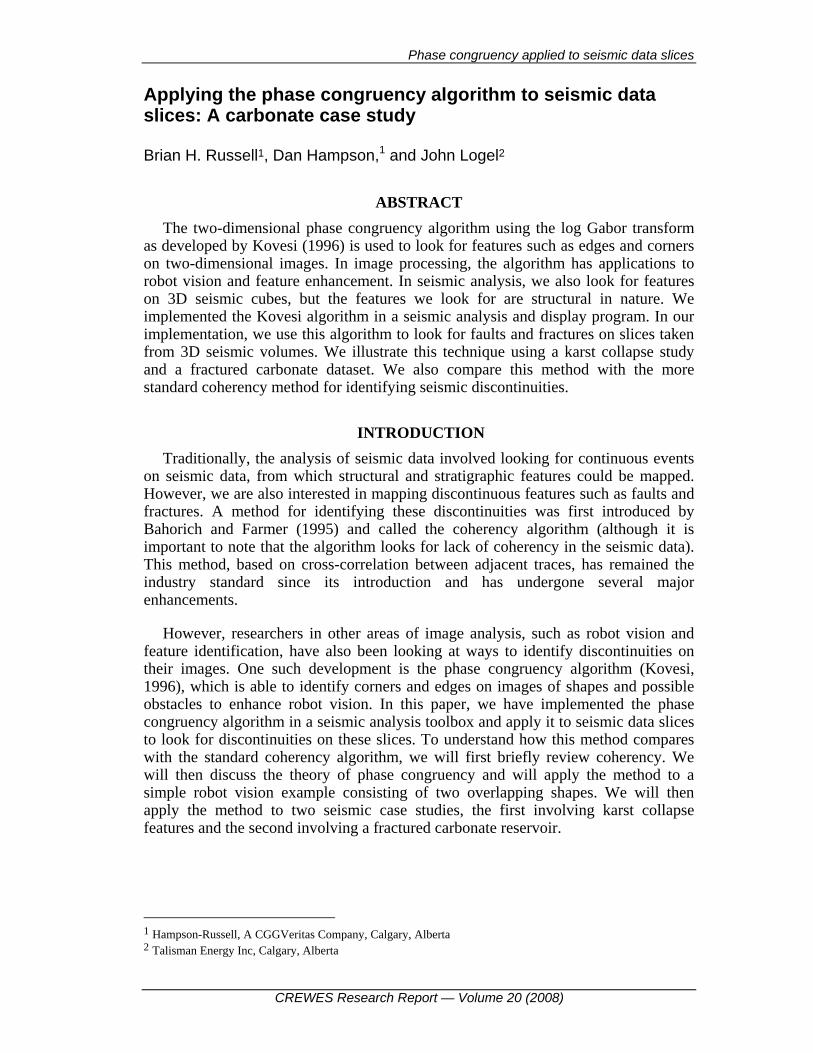
FIG. 10. Map views of all 24 combinations of radial and angular filters applied in this example, where (a) shows the filters at all angles for the first scale (Scale0), (b) shows the filters at all angles for the second scale (Scale1), (c) shows the filters at all angles for the third scale (Scale2), and (d) shows the filters at all angles for the last scale (Scale3).

Finally, Figure 10 shows the 24 individual filters, in groups of six corresponding to the angle range for each scale.

At this point, we could continue in this manner, showing the Fourier transforms and their inverses at each step of the analysis. However, this would be quite tedious and not very instructive. The key thing to understand is the when the filters in Figure 10 are applied and their inverse transforms are computed, we stack over the scales for each angle and then apply moment analysis. The final result is shown in Figure 11(b), with the initial image shown in Figure 11(a) for reference. Notice how well that the edges of the two structures have been defined.

(a) (b)

FIG. 11. Map views of the (a) original image consisting of a cylinder and a cube from figure 5(b), and (b) the final analysis using phase congruency. Notice the clear definition of the edges of the two objects.

Of course, the example shown in this section is extremely simple and also not

representative of the type of image we want to analyze on our seismic slices. Thus, in the following sections, we will implement the phase congruency algorithm on seismic data slices.

IMPLEMENTATION ON 3D SEISMIC VOLUMES To apply the phase congruency algorithm to seismic data slices, we first had to

find a way to feed seismic data slices to the program. This could have been done either by exporting the data slices in a format understood by the Kovesi MATLAB program (Kovesi, 1996-2003) or by converting his MATLAB code to a format in which the data slices were in natural format. We chose the latter option, converting the MATLAB code to C++ code in the Hampson-Russell seismic analysis suite of



programs. Thus, phase congruency becomes one option in a series of options for analyzing seismic data.

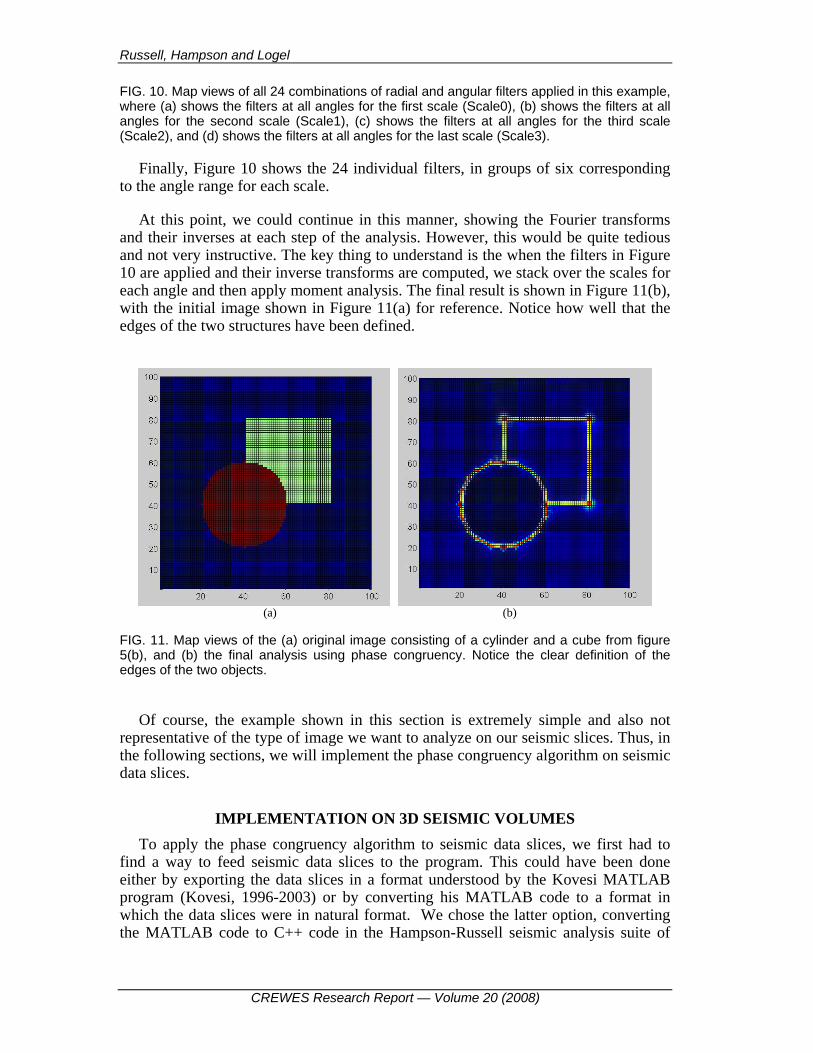
A simple schematic diagram showing the way in which the phase congruency method was implemented on seismic data is shown in Figure 11. Although this algorithm proceeds by analyzing constant time slices, it should also be possible to apply the algorithm to structural, or stratigraphic, slices.

FIG. 12. A schematic showing the implementation of the phase congruency algorithm to seismic data.

We will now implement the phase congruency algorithm on several seismic examples. The first example will be a Karst collapse study from Boonsville, Texas, and the second example will be from a fractured carbonate reservoir in Alberta.



KARST COLLAPSE CASE STUDY We will first analyze a 3D dataset from the Boonsville area of north Texas. The

wells and 3D seismic from this dataset are public domain, and available from the Bureau of Economic Geology at the University of Texas. A map of the area is shown in Figure 13.

FIG. 13. A map showing the location of the Boonsville gas field. (Hardage et al., 1996).



The geology of the area and exploration objectives of the Boonsville dataset have been fully described by Hardage et al. (1996). To illustrate the geology, a representative seismic section from this paper is shown in Figure 14.

A B C

FIG. 14. A representative seismic section from the 3D Boonsville dataset, with the producing horizons numbered from 1 to 4, and the Karst collapse features identified by the ellipses. This line is reconstructed at the points A, B and C on the survey as indicated in Figure 16(a) (from Hardage et al., 1996).

In the Boonsville gas field, production is from the Bend conglomerate, a middle Pennsylvanian clastic deposited in a fluvio-deltaic environment. In Figure 14, the top of the Bend formation is indicated by event 1 at 850 ms, the Caddo, and the base of the Bend is indicated by event 4 at 1050 ms, the Vineyard.

The Bend formation is underlain by Paleozoic carbonates, the deepest being the Ellenburger Group of Ordovician age. The Ellenburger contains numerous karst collapse features which extend up to 760 m from basement through the Bend conglomerate. As can be seen in Figure 14, these Karst collapse features, illustrated by the vertical ellipses, have a significant effect on the basal Vineyard event and continue vertically almost until the top Caddo event.



A schematic drawing of a typical Karst collapse feature is shown in Figure 15. This figure was adapted by Hardage et al. (1996) from work done by Lucia (1995) using Ellenburger outcrops in the El Paso region.

FIG. 15. A schematic of a karst collapse feature. (Hardage et al., 1996, adapted from Lucia, 1995).

The karst collapse features are also evident when we look at the amplitude and time structure maps from the Vineyard (base Bend conglomerate) horizon (event 4 on the seismic section in Figure 14), as shown in Figure 16. The circular white areas in the amplitude map of Figure 16(a) clearly show these Karst collapse features, as do the circular structures of the time structure map of Figure 16(b). In Figure 16(a) the reconstructed seismic profile of Figure 14 is shown by the points A, B and C. Also, in both figures, the white rectangle indicates the extent of the public domain 3D survey which will be analyzed next. Hardage et al. (1996) demonstrate, using measured pressure data, that these karst collapse features affect reservoir compartmentalization within the producing Bend formation.



(a) (b)

FIG. 16. Maps of (a) amplitude and (b) time structure from the Vineyard event (event 4) on Figure 14, where the black line A-B-C shows the seismic profile from Figure 13 and the white box on each figure shows the extent of the public 3D survey analyzed in the next figure (from Hardage et al., 1996).

It is therefore important to identify the karst collapse features from the seismic

volume, and we will do this using both the phase congruency and coherency methods. Figure 17 shows a set of composite slices (in the X, Y and Z directions) over the 3D seismic survey illustrated by the white outline in Figures 16(a) and (b), where Figure 17(a) shows the original seismic survey and Figure 17(b) shows the phase congruency results. On Figure 17(a), the Y-direction, or in-line, slice shows the karst features quite clearly (they are annotated with the red ellipses) but on the horizontal time slice they are not as clear. On Figure 17(b), the in-line slice shows the karst features even more clearly than on the seismic display (again, they are annotated with the red ellipses) and on the horizontal time slice they are also much clearer.

(a) (b)

FIG. 17. A vertical slice showing karst features superimposed on a horizontal slice at 1080 ms, roughly halfway through the karst collapse, where (a) shows the seismic volume and (b) shows the phase congruency volume.



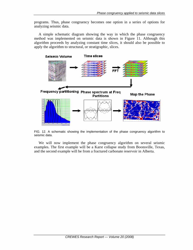
Figure 18 shows the same set of composite slices (in the X, Y and Z directions) as in Figure 17, where Figure 18(a) again shows the original seismic survey and Figure 18(b) now shows the coherency results.

(a) (b)

FIG. 18. A vertical slice showing karst features superimposed on a horizontal slice at 1080 ms, roughly halfway through the karst collapse, where (a) shows the seismic volume and (b) shows the coherency volume.

On Figure 18(b), the in-line slice shows the karst features more clearly than on the

seismic display (again, they are annotated with the red ellipses) than on the seismic display, but slightly less clearly than on the phase coherency.

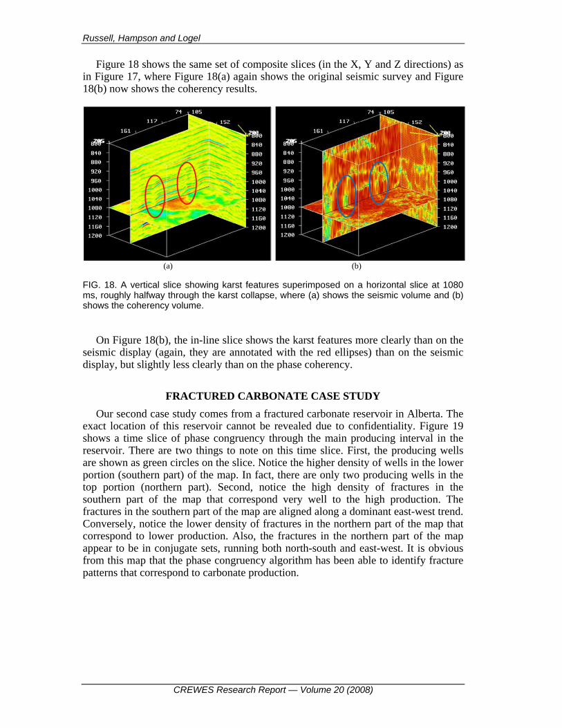
FRACTURED CARBONATE CASE STUDY Our second case study comes from a fractured carbonate reservoir in Alberta. The

exact location of this reservoir cannot be revealed due to confidentiality. Figure 19 shows a time slice of phase congruency through the main producing interval in the reservoir. There are two things to note on this time slice. First, the producing wells are shown as green circles on the slice. Notice the higher density of wells in the lower portion (southern part) of the map. In fact, there are only two producing wells in the top portion (northern part). Second, notice the high density of fractures in the southern part of the map that correspond very well to the high production. The fractures in the southern part of the map are aligned along a dominant east-west trend. Conversely, notice the lower density of fractures in the northern part of the map that correspond to lower production. Also, the fractures in the northern part of the map appear to be in conjugate sets, running both north-south and east-west. It is obvious from this map that the phase congruency algorithm has been able to identify fracture patterns that correspond to carbonate production.



FIG. 19. A time slice of phase coherency within the reservoir interval of a carbonate reservoir in Alberta, where the yellow circles represent producing wells.

Next, Figure 20 shows a vertical seismic section on the left along the result of

analysis with three different algorithms: an un-named contractor section which attempts to display fracture density, phase congruency, and curvature. (Curvature is an attribute that we have not discussed in this paper. For more details on curvature, see Roberts (2001)).

On the three computed fracture plots an FMI, or Formation MicroImager, log curve has been superimposed, showing the density of fractures. Note that this log does not correlate well with the commercial product, but shows good correlation with both the phase congruency and curvature plots. In particular, the green colour indicates large values of both phase congruency and curvature in both plots and corresponds to large values of fracture density on the FMI log.



FIG. 20. The seismic section on the left and, from left to right: a contractor section that computes fracture density, phase congruency and curvature. Superimposed on the three computed sections on the right is an FMI, or Formation MicroImager, log that measures fracture density.

Finally, Figure 21 shows a plot of initial production (in cubic metres) versus amplitude of phase congruency, computed over six wells. As can be seen in this plot, there is a roughly linear trend between initial production and the amplitude of the phase congruency. In other words, higher phase congruency correlates with more fractures and more fractures correlates with more production.

Amplitude of Phase Congruency vs. Initial Production

2043.1

3860.9

1295

1909

2827

2215

0

500

1000

1500

2000

2500

3000

3500

4000

4500

0 0.5 1 1.5 2 2.5 3 3.5 4

Phase Congruency Total Amplitude

Initi

al P

rodu

ctio

n (m

3)

3-1214-128-1215-72-76-7

FIG. 21. A crossplot of initial production from the carbonate reservoir with phase congruency amplitude.



CONCLUSIONS In this paper, we implemented a new scheme for identifying discontinuities on

seismic data slices, called phase congruency. As we discussed, the phase congruency approach has found application in the identification of features on images and is used in image processing for robot vision. However, the method had found little application in the seismic area and so we decided to see if it could aid in the search for discontinuities on seismic time slices. After a discussion of the coherency method, which is the generally accepted method for identifying seismic discontinuities, we then described the theory of the phase congruency method. Next, we showed how the method works on a simple image consisting of an overlapping cylinder and cube. Finally, we applied the algorithm to two seismic examples, comparing its results with other seismic techniques such as coherency and curvature.

In our first seismic example, a karst collapse study from the Boonsville field in Texas, we found that phase congruency did a good job in identifying these karst features. From an economic standpoint, the identification of the karst features was of great interest since it lead to the identification of compartmentalization in the reservoir interval above the karst collapse zones.

Our second seismic example was a fractured carbonate reservoir from Alberta. We found that the phase congruency method was able to identify the areas in the field in which maximum fracturing had occurred. These areas of high fracturing in turn correlated with the highest initial production values in the field. When amplitude of phase congruency was plotted against initial production, a good correlation was found.

In this study, we found that other attributes such as coherency and curvature also performed well. However, the phase congruency method when applied to seismic slices gives a new and different seismic discontinuity attribute, one that can add value to ongoing seismic exploration and production efforts.

ACKNOWLEDGEMENTS We wish to thank our colleagues at the CREWES Project, CGGVeritas and Talisman for their support and ideas, as well as the sponsors of the CREWES Project.

REFERENCES Bahorich, M. and Farmer, S., 1995, 3-D seismic discontinuity for faults and stratigraphic features: The

coherence cube: The Leading Edge, 14, no. 10, 1053-1058. Cook, J., Chandran, V. and Fookes, C., 2006, 3D face recognition using log-Gabor templates:

presented at the British Machine Vision Conference (BMVC), September 4-7, 2006, Edinburgh.

Field, D., 1987, Relations between the statistics of natural images and the response properties of cortical cells: Journal of the Optical Society of America, vol. 4, no. 12, pp 2379-2394.

Gersztenkorn, A. and Marfurt, K. J., 1999, Eigenstructure-based coherence computations as an aid to 3-D structural and stratigraphic mapping: Geophysics, 64, 1468-1479.

Hardage, B.A., Carr, D.L., Lancaster, D.E., Simmons, J.L. Jr., Elphick, R.Y., Pendleton, V.M. and Johns, R.A., 1987, 3-D seismic evidence of the effects of carbonate karst collapse on



overlying clastic stratigraphy and reservoir compartmentalization, Geophysics, 61, 1336-1350.

Kovesi, P.D., 2003, Phase congruency detects corners and edges: Proceedings of the Seventh Australasian Conference on Digital Image Computing Techniques and Applications (DICTA’03).

Kovesi, P.D., 1996-2003, MATLAB functions for computer vision and image analysis: http://www.csse.uwa.edu.au/~pk/Research/MatlabFns/.

Kovesi, P.D., 1996, Invariant Measures of Feature Detection: Ph.D. thesis, The University of Western Australia.

Lucia, F.J., 1995, Lower Paleozoic cavern development, collapse and dolomitization, Franklin Mountains, El Paso, Texas, in Budd, D.A., Saller, A.H., and Harris, P.M., Eds., Unconformities and porosity in carbonate strata: AAPG Memoir 63, 279-300.

Marfurt, K. J., Kirlin, R. L., Farmer, S. L. and Bahorich, M. S., 1998, 3-D seismic attributes using a semblance-based coherency algorithm: Geophysics, 63, 1150-1165.

Roberts, A., 2001, Curvature attributes and their application to 3D interpreted horizons: First Break, 19, 86-100.

applying the phase congruency algorithm to seismic data slices: … · 2020-01-17 · applying the...

Documents