Applying Portfolio Theory to Timber Product

by

SHAZUIN BINTI SHAHRI

Dissertation submitted in partial fulfillment of the requirements for the degree of Master of Science in Statistics

April 2009

ACKNOWLEDGEMENT

I would like to acknowledge Associate Professor Adam Baharum who

supervised me on the project. His support guided me to the end. My warmest thanks go

to Dr. Adli Mustafa and all academic and non-academics staff of School of

Mathematical Science, USM.

I thank my friends, postgraduate classmates and colleagues for their

encouragements and guidance. To my parents, thank you for your support and

encouragement.

Finally and the most of all, I want to acknowledge Allah S.W.T. He teaches

everything.

SHAZUIN BINTI SHAHRI

11

4.2 4.3 4.4 4.5 4.5

Data Generation Descriptive Statistics The Mean-Variance (MY) Efficiency The MY Efficiency Frontier The Semi-Variance Model

CHAPTER5 : RESEARCH FINDING AND DISCUSSION

5.1 5.2

Introduction Discussion 5.2.1 The Mean-Variance (MY) Efficiency 5.2.2 The MV Efficiency Frontier 5.2.3 The Semi-Variance Model

CHAPTER6 : CONCLUSION AND RECOMMENDATION

6.1 6.2 6.3 6.4

Introduction Conclusion Limitation of the Study Recommendation for Future Study

REFERENCES

APPENDICES

Appendix 1: Peninsular Malaysia: Export of Major Timber Product and FOB Value per Volume (RMlM3) (2001 - 2008 Q3)

Appendix 2: Peninsular Malaysia: Export of Sawn Timber to Major Destination and FOB Value per Volume (RMlM3) (2000-2008 Q3)

Appendix 3: Lingo Program Model for Portfolio Return on Six Major Timber Product

Appendix 4: Lingo Program Model for Generating Point along the Efficient Frontier on Six Major Timber Product

Appendix 5: Lingo Program Model for Minimizing Semi-variance on Six Major Timber Product

IV

31 32 38 40 41

45 45 45 46 48

49 49 50 50

52

Table 4.1:

Table 4.2:

Table 4.3:

LIST OF TABLES

Growth in value per unit volume for six timber products over seven-year period

Covariance matrix between six timber products

Expected return for six timber product for the period of seven years

Table 4.4: Correlation matrix between six timber products

Table 4.5: Growth in value per unit volume for export of sawn timber to fifteen major destinations over eight-year period

Table 4.6: Covariance matrix between exports of sawn timber to fifteen major destinations

Table 4.7: Expected return for exports of sawn timber to fifteen major destinations

Table 4.8: Correlation matrix between exports of sawn timber to fifteen major destinations

Table 4.9: Program Output for Portfolio Return on Six Major Timber Products

Table 4.10: Program Output for Portfolio Return on Export on Sawn Timber to Major Destination

Table 4.11: The Point Generated along Efficient Frontier for SIX

timber products

Table 4.12: The Point Generated along Efficient Frontier for export of Sawn Timber to Major Destination

Table 4.13: Program Output for Minimizing Semi-Variance for Six Timber Products

Table 4.14: Program Output for Minimizing Semi-Variance for export of Sawn Timber to Major Destination

v

Pages

32

32

33

33

34

35

36

37

38

39

40

41

42

4

Figure 3.1:

Figure 5.1:

Figure 5.2:

LIST OF FIGURES

Efficient Frontier. The hyperbola is sometimes referred to as the 'Markowitz Bullet'

Timber Product Efficiency Frontier

Export of Sawn Timber to Major Destination Efficiency Frontier

VI

Pages

27

46

47

APLIKASI TEORI PORTFOLIO KEP ADA PRODUK BALAK

ABSTRAK

Sejak seminar analisis min-varians diperkenalkan oleh Markowitz (1952), teori

portfolio telah diperkembangkan dalam konteks model pilihan normatif, termasuk

bagaimana untuk membentuk portfolio yang optimum.

Analisis ini menggunakan teori portfolio untuk mendapatkan penyelesaian

optimum, memaksimumkan keuntungan dan meminimumkan risiko bagi produk balak

di Semenanjung Malaysia dan eksport satu produk balak terpilih ke destinasi utama

dunia. Masalah ini adalah aplikasi secara langsung pendekatan min-varians Markowitz

dan masalah pengoptimuman portfolio dapat diformulakan sebagai pengaturcaraan

matematik.

Data berkenaan produk balak dianalisis untuk menghasilkan mm-varlans

efisyensi. Kemudian, kecekapan frontier dihasilkan untuk memastikan pulangan risiko­

teritlak optimum bagi portfolio tersebut. Akhir sekali, model semi-varians dijanakan

untuk menghasilkan nilai optimum dan perbandingan dengan model min-varians

dilaksanakan.

Vll

ABSTRACT

Since the seminal mean-variance analysis was introduced by Markowitz (1952),

the portfolio theory has been expanded in the context of normative choice modeling,

including how to form an optimal portfolio.

This study uses portfolio theory to find the optimal, profit maximizing and risk­

minimizing combinations of timber product in Peninsular Malaysia and the export of

one selected timber product to major destination throughout the world. This problem is a

straight forward application of Markowitz mean-variance approach and the optimal

portfolio problem can be formulated as mathematical programming.

The data on timber product was analyzed to create mean-variance efficiency.

Then, an efficiency frontier was created to ensure optimal risk-adjusted returns of the

portfolio. Finally, a semi-variance model was run to generate the optimal values and to

make comparison with the mean-variance model.

Vlll

1.1 Introduction

CHAPTER 1

INTRODUCTION

Financial economics, mathematics, management theory and operations research

have derived several techniques to value portfolios. Formal portfolio theory research

saw major advances in the context of normative choice modeling, including how to form

an optimal portfolio, beginning with Harry Markowitz (1959).

Researchers and portfolio analysts have spent considerable effort developing

models showing the appropriate mix of equity investments to optimize risk-adjusted

returns. These optimal portfolios often have a mix of stocks, bonds, and cash, often

including an international component used to reduce risk or boost returns. Increasingly,

institutional investors are looking for other alternative investments to increase the return

or lower the risk of their investment portfolios.

A basic premise of economics is that, due to the scarcity of resources, all

economic decisions are made in the face of trade-offs. Markowitz identified the trade-off

facing the investor: risk versus expected return. The investment decision is not merely

which securities to own, but how to divide the investor's wealth amongst securities. This

is the problem of "Portfolio Selection;" hence the title of Markowitz's seminal article

published in the March 1952 issue of the Journal of Finance. In that article and

subsequent works, Markowitz extends the techniques of linear programming to develop

1

the critical line algorithm. The critical line algorithm identifies all feasible portfolios that

minimize risk (as measured by variance or standard deviation) for a given level of

expected return and maximize expected return for a given level of risk. When graphed in

standard deviation versus expected return space, these portfolios form the efficient

frontier. The efficient frontier represents the trade-off between risk and expected return

faced by an investor when forming his portfolio. Most of the efficient frontier represents

well diversified portfolios. This is because diversification is a powerful means of

achieving risk reduction.

Markowitz developed mean-variance analysis in the context of selecting a

portfolio of common stocks. Over the last decade, mean-variance analysis has been

increasingly applied to asset allocation. Product allocation is the selection of a portfolio

of investments where each component is an asset class rather than an individual security.

Mean-variance analysis requires not only knowledge of the expected return and standard

deviation on each asset, but also the correlation of returns for each and every pair of

assets. Whereas a stock portfolio selection problem might involve hundred of stocks

(and hence thousands of correlations), a product selection problem typically involves a

handful of asset classes (for example stocks, bonds, cash, real estate, and marketing

product). Furthermore, the opportunity to reduce total portfolio risk comes from the lack

of correlation across assets. Since stocks generally move together, the benefits of

diversification within a stock portfolio are limited. In contrast, the correlation across

asset classes is usually low and in some cases negative. Hence, mean-variance is a

2

powerful tool in asset allocation for uncovenng large risk reduction opportunities

through diversification.

The relatively small data requirements of applying mean-variance analysis to

product selection along with the speed and low cost of powerful personal computers

(PCs) have led to the commercial deVelopment of many PC-based mean-variance

optimization software packages for use in product selection. Some of these optimizers

do not solve for the entire efficient frontier using the critical line algorithm; instead, they

maximize a parametric objective function in mean and variance for a handful of

parameter values. Other optimizers implement some fonn of the critical line algorithm

to solve for the entire efficient frontier. The latter approach has the advantage that once

the efficient frontier has been found, any number of objective functions with any

number of parameter values can be optimized without having to rerun the algorithm.

1.2 Assumptions of Mean-Variance Analysis

As with any model, it is important to understand the assumptions of mean­

variance analysis in order to use it effectively. First of all, mean-variance analysis is

based on a single period model of investment. At the beginning of the period, the

investor allocates his wealth among various asset classes, assigning a nonnegative

weight to each asset. During the period, each asset generates a random rate of return so

that at the end of the period, his wealth has been changed by the weighted average of the

returns. In selecting asset weights, the investor faces a set of linear constraints, one of

which is that the weights must sum to one.

3

Based on the game theory work of Von Neumann and Morgenstern, economic

theory postulates that individuals make decisions under uncertainty by maximizing the

expected value of an increasing concave utility function of consumption. In a one period

model, consumption is end of period wealth. In general, maximizing expected utility of

ending period wealth by choosing portfolio weights is a complicated stochastic

nonlinear programming problem. Markowitz asserted that if the utility function can be

approximated closely enough by a second-order Taylor expansion over a wide range of

returns then expected utility will be approximately equal to a function of expected value

(mean) and variance of returns. This allows the investor's problem to be restated as a

mean-variance optimization problem so that the objective function is a quadratic

function of portfolio weights.

The utility function is assumed to be increasing and concave because we assume

that (1) investors prefer more consumption to less, and (2) investors are risk averse. In

terms of the approximating utility function, this translates into expected utility being

increasing in expected return (more is better than less) and decreasing in variance (the

less risk the better). Hence, of all feasible portfolios, the investor should only consider

those that maximize expected return for a given level of variance, or minimize variance

for a given level of expected return. These portfolios form the mean-variance efficient

set.

4

1.3 Assumption to Application of Portfolio Selection

We consider portfolio selection when the following three conditions are

satisfied:

1. The investor owns only liquid assets.

11. He maximize the expected value of U(C1, C2, ••• , CT), where CT is the

money value of consumption during the ith period (CT could,

alternatively, represent money expenditure deflated by a cost of living

index).

lll. The set of available probability distributions of returns from portfolios

remains the same through time (if CT is deflated consumption, then it is

'real return', taking into account changes in price level whose probability

distribution is assumed constant).

Later, we consider modifications of these assumptions.

An asset is perfectly liquid if

IV. The price at which it can be sold, at a particular time, always equals the

price at which it can be bought at that time; and

v. Any amount can be bought or sold at this price.

Even though securities are not perfectly liquid, they are sufficiently liquid for an

analysis based on liquidity to be instructive. The effects of illiquidities, among other

things, are consider later.

5

Conditions (iii) does not imply that the same security offers the same

opportunities at all times. The new and promising firm of today may be a well­

established or a defunct firm tomorrow - at which time the role of being 'new and

promising' is taken over by other firms. The assumption, made at first and modified

later, is that the opportunities from the market as a whole remain constant.

Perfectly, liquid assets may be converted into cash, and cash may be converted

into liquid assets without loss. If available probability distributions remain the same

through time, the investor's opportunities depend only on the value of his portfolio. If

we let Yt+I be the value of the portfolio at the beginning of period t + 1 (i.e. at the end of

period t), then, under our present assumptions, the single period utility function

U = U ((Ct, Wt+!, Ct , C2, ••. , Ct-1 )

can be written as

U = U ((Ct, Yt+l, C1, C2, ••. , Ct-t)

1.4 Objectives of a Portfolio Analysis

It is impossible to derive all possible conclusion concerning portfolios. A

portfolio analysis must be based on criteria which serve as a guide to the important and

unimportant, the relevant and irrelevant.

The proper choice of criteria depends on the nature of the investor. For some

investors, taxes are a prime consideration; for others, such as non-profit corporations,

they are irrelevant. Institutional considerations,)egal restrictions, relationship between

6

portfolio returns and the cost of living may be important to one investor and not to

another. For each type of investor, the details of the portfolio analysis must be suitably

selected.

Two objectives, however, are cornmon to all investors for which the techniques

are design:

1. They want return to be high, the appropriate definition of return may vary

from investor to investor. But, in what sense is appropriate, they prefer

more of it to less of it.

11. They want return to be dependable, stable, not subject to uncertainty. No

doubt there are security purchasers who prefer uncertainty, like bettors at

a horse race who pay to take chances. The techniques are not for

speculators. The techniques are for the investors who, other things being

equal, prefer certainty to uncertainty.

The portfolio with highest likely return is not necessarily the one with least

uncertainty of return. The most reliable portfolio with an extremely high likely return

may be subject to an unacceptably high degree of uncertainty. The portfolio with the

least uncertainty may have an undesirably small likely return. Between these extremes

would lay portfolios with varying degrees of likely return and uncertainty.

The proper choice among efficient portfolios depends on the willingness and

ability of the investor to assume risk. If safety.is of extreme importance, likely return

7

must be sacrificed to decrease uncertainty. If a greater degree of uncertainty can be

borne, a greater level of likely return can be obtained. An analysis presented here are:

First, separate efficient portfolios from inefficient one's;

Secondly, portrays the combinations of likely return and uncertainty of return available

from efficient portfolios;

Thirdly, the investors or investment manager carefully select the combination of likely

return and uncertainty that best suits his needs; and

Lastly, detennine the portfolio which provides the most suitable combinations of risk

and return.

1.5 Illustration of Mean-Variance Analysis

To illustrate mean-variance analysis as it applies to asset allocation, consider an

investor whose portfolio is entirely in the U.S. capital markets but is considering going

into non-U.S. markets. The first step of the analysis is to divide the world capital

markets into broad asset classes. In this example, we have four portfolios: U.S. stocks,

non-U.S. stocks, U.S. bonds, and non-U.S. bonds. The second step is to develop capital

market assumptions; namely, expected returns and standard deviations for each asset

class and correlations between each pair of asset classes. These assumptions are usually

derived from historical data on asset class returns and current market conditions. The

third step is to generate the efficient frontier by running the critical line algorithm.

Markowitz showed that while there are infinitely many efficient portfolios, you only

need a limited number of comer portfolios to identify all efficient portfolios. Not all

efficient portfolios contain all assets. Moving, along the efficient frontier, a comer

8

portfolio is located where an asset weight or slack variable is either added or dropped.

Every efficient portfolio is a linear combination of the two comer portfolios

immediately adjacent to it. Thus, by locating all comer portfolios, the critical line

algorithm generates the entire efficient frontier.

1.6 Background of the Study

This study will focus on application of portfolio theory to improve return to

timber product selection and distribution to major destination. Data were obtained from

Malaysian Timber Council and are accessible through the website

http://www.mtc.com.my/info/index.php?option=com content&view=category&id=44&

Itemid=63 . There are 13 major products available for exports which are logs, sawn

timber, sleepers, veneer, mouldings, chipboard/particleboard, fibreboard, plywood,

wooden frame, builders joinery & carpentry, wooden furniture, rattan furniture and also

others timber products.

The data are available from 1994 to third quarter of 2008. However the complete

data set is available for 2002 to selected timber product with volume and FOB (freight

on board) value.

For this study, we will focus onsix (6) major products i.e. sawlogs, sawn timber,

sleepers, veneer, mouldings and fibreboard, with export Freight on Board value obtained

from Peninsular Malaysia. Later, we will focus on one selected timber product i.e. sawn

9

timber to analyze the returns to fifteen (15) major destinations by using the same method

as constructed for the first data set, which were taken from 2001 to third quarter 2008.

1.7 Objectives of the Study

The objectives of the study are as follows:

• To minimize the end-of-period variance in portfolio selection

• To generate points along the efficient frontier

• To minimize the semi-variance in the portfolio selection

10

2.1 Introduction

CHAPTER 2

LITERATURE REVIE\V

Timber product selection is timely, important, and essential in Malaysia, since

public and private companies continue to produce higher-volume of timber product over

the time. In this study, timber can be considered as product for investors and also as

forest/timber plantation which can be utilised by logging operators.

A 'portfolio' is defined simply as a combination of items: securities, assets, or

other objects of interest. Portfolio theory is used to derive efficient outcomes, through

identification of a set of actions, or choices, that minimize variance for a given level of

expected returns, or maximize expected returns, given a level of variance. Decision

makers can then use the efficient outcomes to find expected utility-maximizing solutions

to a broad class of problems in investment, finance, and resource allocation (Robison

and Brake, 1979). Simply put, portfolio theory can be used to maximize profits and

minimize risk in a wide variety of settings and choices, including timber product

selection in Peninsular Malaysia.

A literature on product selection and variety adoption decisions exists, as

reported by Cardozo and Smith (1983) that said, "Results indicate that financial

portfolio theory has promise an analytical and planning tool for product portfolio

decisions, and suggest how action recommendations based on financial portfolio theory

11

may be modified for product portfolio decisions." Leong and Lim (1991) informed that

multiperiod portfolio framework should help marketers in allocating scarce corporate

resources to various competing products as well as contribute to develop a body of

theory to solve an important problem in marketing management.

Seminal works on plantations begin with Griliches (1957), who evaluated the

determinants of hybrid com adoption in the United States. Heisey and Brennan (1991)

studied the demand for wheat replacement seed in Pakistan, and Traxler et al. (1995)

documented and analyzed the steady growth of yields of new wheat varieties in Mexico.

Smale, Just, and Leathers (1994) summarized several explanations for a relatively slow

adjustment to a newly introduced variety, including input fixity and portfolio selection.

The use of mixtures of varieties portfolios has also been studied from ecological and

pathological perspectives. Garrett and Cox (2008) reported that, "The construction of

crop variety mixtures is an example of a technology that draws heavily on ecological

ideas and has also contributed to our understanding of disease ecology through

experiments that examine the effects of patterns of host variability on disease through

time and space" (pp. 1-2).

The study of decision making under risk has a long history, beginning with early

decision models of resource allocation that maximized expected returns. Portfolio theory

significantly improved our ability to analyze and identify optimal choices under risk by

extension of the analysis to include variability, as well as expected returns. Portfolio

12

theory was initially developed by Markowitz (1959) and Tobin (195X). with extensions

by Lintner (1965) and Sharpe (1970).

Financial portfolio analysis provides a useful framework for conceptualizing

product selection decisions, and implementing variety strategies and producl decisions.

Variety choices are similar to investment decisions in financial markets, where fillancial

managers allocate money across investment opportunities with relative risks alld returns

across a set of correlated assets. Since different varieties of product respond differelllly

to environmental conditions, the risks associated with product selection are correlakd.

Some product will be positively related to other product, and some may be negatively

correlated with other products. Because of this correlation, or relationship, there arc

potential benefits by considering investment in multiple product selection.

The application of portfolio theory to product decisions is new, but applications

of portfolio theory to risky decisions in agriculture and timberland allocation has been

around for a long time. Collins and Barry (1986) applied Sharpe's (1970) extension of

the Markowitz model to a 'single index' portfolio model to study diversification of

agricultural activities. The single index model does not require a complete, balanced

data set, and is computationally less demanding. Turvey et aI. (1985) compared a full

variance-covariance (Markowitz) model to a single index model in a case farm in

southern Ontario, and found that the single index model a practical alternative III

applications to the complete model for deriving mean-variance efficient farm plans.

13

Robison and Brake (1979) provided a thorough and informative literature review

of portfolio theory, with applications to agriculture and agricultural finance. Barry

(1980) extended portfolio theory to the Capital Asset Pricing Model (CAPM), and

applied the model to farm real estate. More recently, Nyikal and Kosura (2005) used

quadratic programming (QP) to solve for the efficient mean-variance frontier to better

understand farming decisions in Kenyan agriculture. Another recent application of

portfolio theory was conducted by Redmond and Cubbage (1988), who applied the

capital asset pricing model (CAPM) to timber asset investments in the United States.

Figge (2002) summarized the literature on how portfolio theory has been applied to

biodiversity, and Sanchirico et al. (2005) use portfolio theory to develop optimal

management of fisheries.

The portfolio approach used in these previous studies will be applied to timber

product selection and the distribution of a single product to major destination through

out the world.

2.2 Mean - Variance (MV) Efficiency

The model used to estimate the efficiency frontier for product selection is the

model developed by Markowitz to study investments, and later applied to timber product

selection in Peninsular Malaysia.

Markowitz (1959) developed portfolio theory as a systematic method of

minimizing risk for a given level of expenditur~. To derive an efficient portfolio of

14

timber product selection, measures of expected returns (average product) and variance

of product are required for each product, together with all of the pairwise covariances

across all products. The efficient mean-variance frontier for a portfolio of timber product

is derived by solving a sequence of quadratic programming problems. Based on an

investor's preferences for higher return and less risk, a particular point on the efficiency

frontier can be identified as the 'optimal' portfolio of product selection.

We assume that a timber producer or timber investor is given total volume (X),

and desires to choose the optimal allocation of timber product selection. Thus the

decision variable is, Xi the percentage of total volume allocated to selection i, where i =

1, ... , n, and LXi = X Quadratic programming is used to solve for the efficiency i=i

frontier of mean-variance (MV) combinations. This frontier is defined as the maximum

mean for a given level of variance, or the minimum variation for a given Xi mean

product. If we define yi as the mean product of selection i, then the total product is

simply the weighted average product, that is L XiYi .

i=i

The variance of total timber selection for the entire product (V) is defined in

equation (1),

(2.1)

where:

15

Xj is the level of activity j, which is the percentage of volume allocated

to productj,

(Jjk is the covariance of selection between the jth and kth product

selection, and equal to variance when j = k.

Hazell and Norton (1986) emphasize the intuition embedded in equation (1): the

total variance product or varieties allocated (V) is an aggregate of the variability of

individual varieties and covariance relationships between the products. Two conclusions

are useful to better understand the portfolio approach to timber product selection:

(i) Combinations of product that have negative covariate selection will result in

a more stable aggregate selection for the entire farm than specialized

strategies of allocating single varieties, and

(ii) A product that is risky in terms of its own variance may still be attractive if

its returns are negatively covariate with other product chosen.

The mean-variance efficiency frontier is calculated by minimizing total variance

(V) for each possible level of mean product or yields (yi), as given in equation (2).

Minimize V= 2: j 2: kXjXk(Jjk' ;=1

subject to:

2:XjYj = 1 and ;=1

16

(2.2)

(2.3)

Xj~ 0 for allj (2.4)

The sum of the mean product in equation (3) is set equal to the parameter )"'

defined as the target product level, which is varied over the feasible range to obtain a

sequence of solutions of increasing mean product and variance, until the maximum

possible mean product is obtained.

Equation (2) is quadratic in Xj, resulting in the use of the Lingo Release 11.0.0.23

program to solve the nonlinear equation. The tool uses the nonlinear optimization code

available through example in the program and through its website at www.lindo.com .

Chapter 4 will describe the data utilized in the portfolio model.

17

CHAPTER 3

METHODOLOGY

3.1 Introduction

In this chapter, the chosen methodology for the purposes of this study will be

discussed. Section 3.2 will define the descriptive statistics. Section 3.3 will define the

Mean - Variance (MV) Efficiency Analysis together with the assumptions pertaining to

this case. Subsequently in Section 3.4, the efficient - frontier generated will be defined

while taking into account the selected assumptions. Next, Section 3.5 will discuss the

semi-variance model as a measure of risk and finally in Section 3.6 a method will be

selected to solve the problem.

3.2 Descriptive Statistics

3.2.1 Mean and variance

The mean or arithmetic mean is the standard average, often simply called the

mean. It can be written as

- I n

X=- 2: Xi n i=l

where Xi is the observed value

i = 1,2,3 ... , n

The mean is the arithmetic average of a set of values, or distribution; however,

for skewed distributions, the mean is not necessarily the same as the middle value ,

(median), or the most likely (mode). For example, if the mean income of a group of

18

people is skewed upwards by a small number of people with very large incomes, the

majority of people will have incomes lower than the mean. By contrast, the median

income is the level at which half the population is below it and half is above. The mode

income is the most likely income, and favors a larger number of people with lower

incomes. The median or mode are often more intuitive measures of such data.

If a random variable X has expected value (mean) )l = E(X), then the variance

Var(X) of X is given by:

This definition encompasses random variables that are discrete, continuous, or

neither. Of all the points about which squared deviations could have been calculated, the

mean produces the minimum value for the averaged sum of squared deviations.

The variance of random variable X is typically designated as Var(X), or simply

(32 (pronounced 'sigma squared'). If a distribution does not have an expected value, as is

the case for the Cauchy distribution, it does not have a variance either. Many other

distributions for which the expected value does exist do not have a finite variance

because the relevant integral diverges. An example is a Pareto distribution whose Pareto

index k satisfies 1 < k:S 2.

3.2.2 Correlation

In probability theory and statistics, correlation (often measured as a correlation

coefficient) indicates the strength and direction of a linear relationship between two

19

random variables. That is in contrast with the usage of the term in colloquial speech,

denoting any relationship, which is not necessarily linear. In general statistical usage,

correlation or co-relation refers to the departure of two random variables from

independence. In this broad sense there are several coefficients, measuring the degree of

correlation, adapted to the nature of the data.

A number of different coefficients are used for different situations. The best

known is the Pearson product-moment correlation coefficient, which is obtained by

dividing the covariance of the two variables by the product of their standard deviations.

Despite its name, it was first introduced by Francis Galton.

The correlation coefficient PX,y between two random variables X and Y with

expected values Ilx and Ily and standard deviations o"x and O"y is defined as:

cov (X,Y) E[(X-,ux)(Y-,uy)] p - -X,y - -

O"xO"y O"xO"y (3.1)

where E is the expected value operator and cov means covariance, and

cov (X,Y) is the covariance between two real-valued random variables X

and Y, with expected values ,u x and J1y.

A widely used alternative notation is

corr(X,Y) = Px y

20

and likewise for Y, and since

E[(X - E(X))(Y - E(Y))] = E(XY) - E(X)E(Y),

we may also write

E (XY) - E(X)E(Y) (3.2)

The correlation is defined only if both of the standard deviations are finite and

both of them are nonzero. It is a corollary of the Cauchy-Schwarz inequality that the

correlation cannot exceed 1 in absolute value.

The correlation is 1 in the case of an increasing linear relationship, -1 in the case

of a decreasing linear relationship, and some value in between in all other cases,

indicating the degree of linear dependence between the variables. The closer the

coefficient is to either -1 or 1, the stronger the correlation between the variables.

If the variables are independent then the correlation is 0, but the converse is not

true because the correlation coefficient detects only linear dependencies between two

variables. Here is an example: Suppose the random variable X is uniformly distributed

on the interval from -1 to 1, and Y = X2. Then Y is completely determined by X, so

that X and Yare dependent, but their correlation is zero; they are uncorrelated. However,

in the special case when X and Yare jointly normal, uncorrelatedness is equivalent to

independence.

21

A correlation between two variables is diluted in the presence of measurement

error around estimates of one or both variables, in which case dis attenuation provides a

more accurate coefficient.

3.3 The Mean-Variance (MV) Efficiency

A quadratic utility function can be assumed to be able to describe an investor's

risk / reward preference. This theory thus assumes that only the expected return and the

volatility (i.e., mean return and standard deviation) matter to the investor. To the

investor, other characteristics of the distribution of returns, such as its skewness

(measures the level of asymmetry in the distribution) or kurtosis (measure of the

thickness or so-called 'fat tail '), is of little or no concern.

Volatility, as a proxy for risk, is used as a parameter in this theory, whereas

return is deemed an expectation on the future. This agrees with the efficient market

hypothesis and most of the traditional conclusions in finance such as Black and Scholes

European Option Pricing (martingale measure: which means that the best forecast for

tomorrow is the price oftoday).

Under the model:

Portfolio return is the proportion-weighted combination of the constituent assets'

returns.

22

• Portfolio volatility is a function of the correlation p of the component assets. The

change in volatility is non-linear as the weighting of the component assets

changes.

In general,

• The returns on individual securities or asset rl'r2 , ••• , rn are jointly distributed

random variables, and the return on the portfolio is

n

R= LWJ; (3.3) i=1

and the expected return on the portfolio as a whole is given by:

n

E(r) = L wiE(r; ) (3.4) i=1

where WI is the weighting of component asset i

and fli = E(ri) (3.5)

for i=l,.··,n

• Portfolio variance:

O"~ = Lw}O"}IIwiwjO"iO"jPij (3.6) i=1 i=1 j=1

where i i- j. Alternatively the expression can be written as:

O"~ = IIwiwjO"iO"jPij (3.7) i=1 j=1

where Pif = 1 for i = j.

23

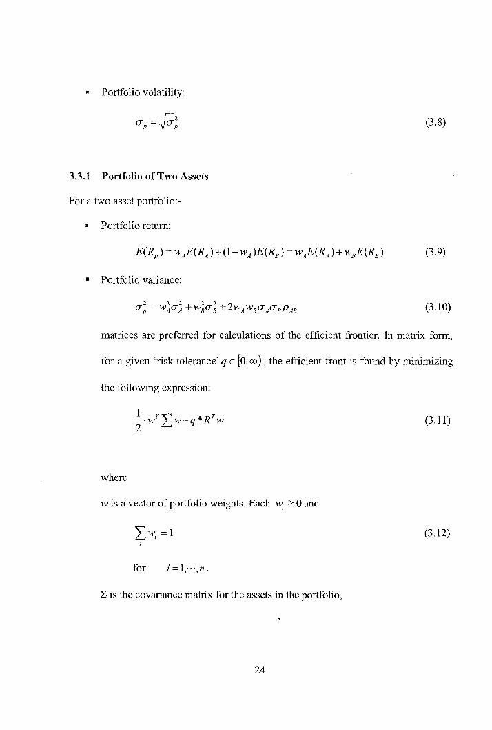
• Portfolio volatility:

(3.8)

3.3.1 Portfolio of Two Assets

For a two asset portfolio:-

Portfolio return:

• Portfolio variance:

(3.10)

matrices are preferred for calculations of the efficient frontier. In matrix form,

for a given 'risk tolerance' q E [0, CI) ), the efficient front is found by minimizing

the following expression:

1 T" T -·w L...Jw-q*R w 2

(3.11)

where

w is a vector of portfolio weights. Each Wi ;::: 0 and

(3.12)

for i = 1,.· ·,n.

L is the covariance matrix for the assets in the portfolio,

24