applied regression analysis - jonathan templin's website · lecture #2 - 1/27/2005 slide 1 of...
TRANSCRIPT

Lecture #2 - 1/27/2005 Slide 1 of 46
Applied Regression Analysis
Lecture 2
January 27, 2005Simple Linear Regression

Overview
Simple Linear Regression
Partitioning the Sum of Squares
Tests of Significance
Assumptions
Diagnostics
Random X
Full Example
SPSS
Wrapping Up
Lecture #2 - 1/27/2005 Slide 2 of 46
Today’s Lecture
■ Simple linear regression.■ Partitioning the sum of squares.■ Tests of significance.■ Assumptions.■ Regression diagnostics (introduction).■ When X is random.■ How to do today’s topics in SPSS.

Overview
Simple Linear Regression
● Small Example
● The Basics
● The Basics
● Estimation
● Example
● Properties
Partitioning the Sum of Squares
Tests of Significance
Assumptions
Diagnostics
Random X
Full Example
SPSS
Wrapping Up
Lecture #2 - 1/27/2005 Slide 3 of 46
Previously on EPSY 581...
Recall from our first meeting the hand calculated sampleproblem with the following scatterplot:
rXY = 0.845
■ Correlation shows the degree of association between X andY ...◆ ...but does so without scale.
■ What if we wanted to predict Y given a value of X?

Overview
Simple Linear Regression
● Small Example
● The Basics
● The Basics
● Estimation
● Example
● Properties
Partitioning the Sum of Squares
Tests of Significance
Assumptions
Diagnostics
Random X
Full Example
SPSS
Wrapping Up
Lecture #2 - 1/27/2005 Slide 4 of 46
The Basics
■ Assume (for now) X is fixed at pre-determined levels in anexperiment - independent variable.
◆ For example, we have an experiment where subjects aregiven X cups of coffee.
◆ Jon the Mad Scientist decides that subjects should berandomly assigned to a group drinking either 1, 2, 3, 4,or5 cups of coffee.
■ The we want to estimate the linear effect of the independentvariable X on the dependent variable Y .
◆ For our example, we want to see how coffee drinkingaffects blood pressure.
◆ Blood pressure = Y = dependent variable.

Overview
Simple Linear Regression
● Small Example
● The Basics
● The Basics
● Estimation
● Example
● Properties
Partitioning the Sum of Squares
Tests of Significance
Assumptions
Diagnostics
Random X
Full Example
SPSS
Wrapping Up
Lecture #2 - 1/27/2005 Slide 5 of 46
The Basics
■ The linear regression model (for observation i = 1, . . . , N ):
Yi = α + βXi + ǫi
■ Don’t be confused by the Greek alphabet, this is simply theequation for a line (y = a + bx).
■ α is the mean of the population when X is zero...the Yintercept.
■ β is the slope of the line, the amount of increase in Ybrought about by a unit increase (X ′ = X + 1) in X.
■ ǫi is the random error, specific to each observation.

Overview
Simple Linear Regression
● Small Example
● The Basics
● The Basics
● Estimation
● Example
● Properties
Partitioning the Sum of Squares
Tests of Significance
Assumptions
Diagnostics
Random X
Full Example
SPSS
Wrapping Up
Lecture #2 - 1/27/2005 Slide 6 of 46
Parameter Estimates
■ Chapter 2 parameterizes the linear regression model as:
Y = a + bX + e
■ To find estimates for a and b consider several possiblechoices:
◆ So thatN
∑
i
|e| is minimized.
◆ So thatN
∑
i
e2 is minimized.
◆ From some guy in the hallway.

Overview
Simple Linear Regression
● Small Example
● The Basics
● The Basics
● Estimation
● Example
● Properties
Partitioning the Sum of Squares
Tests of Significance
Assumptions
Diagnostics
Random X
Full Example
SPSS
Wrapping Up
Lecture #2 - 1/27/2005 Slide 7 of 46
And The Winner Is...
■ Finding a and b that minimize:
N∑
i
e2
■ Using calculus, these happen to be:
b =
∑
(X − X)(Y − Y )∑
(X − X)2= rxy
sy
sx
=
∑
xy∑
x2
■ And:
a = Y − bX
■ LS estimates are considered BLUE: Best Linear UnbiasedEstimators.

Overview
Simple Linear Regression
● Small Example
● The Basics
● The Basics
● Estimation
● Example
● Properties
Partitioning the Sum of Squares
Tests of Significance
Assumptions
Diagnostics
Random X
Full Example
SPSS
Wrapping Up
Lecture #2 - 1/27/2005 Slide 8 of 46
An Example of Simple Linear Regression
■ Table 2.1 in Pedhazur lists data from an experiment where Xwas the number of hours given for study, and Y is the scoreon a test.
1.00 2.00 3.00 4.00 5.00
Hours of Study
4.00
6.00
8.00
10.00
12.00
Te
st
Sco
re
W
W
W
W
W
W
W
W
W
W
W
W
W
W
W
W
W
W
W
W

Overview
Simple Linear Regression
● Small Example
● The Basics
● The Basics
● Estimation
● Example
● Properties
Partitioning the Sum of Squares
Tests of Significance
Assumptions
Diagnostics
Random X
Full Example
SPSS
Wrapping Up
Lecture #2 - 1/27/2005 Slide 9 of 46
Example (continued)
■ We can tell that:◆
∑
(X − X)2 =∑
x2 = 40◆
∑
(X − X)(Y − Y ) =∑
xy = 30◆ X = 3.0◆ Y = 7.3
■ So:
b =
∑
xy∑
x2=
30
40= 0.75
a = Y − bX = 7.3 − (0.75 × 3.0) = 5.05
■ Given these estimates, the linear regression line is given by:
Y ′ = 5.05 + 0.75X

Overview
Simple Linear Regression
● Small Example
● The Basics
● The Basics
● Estimation
● Example
● Properties
Partitioning the Sum of Squares
Tests of Significance
Assumptions
Diagnostics
Random X
Full Example
SPSS
Wrapping Up
Lecture #2 - 1/27/2005 Slide 10 of 46
Example (continued)
1.00 2.00 3.00 4.00 5.00
Hours of Study
4.00
6.00
8.00
10.00
12.00
Te
st
Sco
re
W
W
W
W
W
W
W
W
W
W
W
W
W
W
W
W
W
W
W
W
Test Score = 5.05 + 0.75 * X
R−Square = 0.17

Overview
Simple Linear Regression
● Small Example
● The Basics
● The Basics
● Estimation
● Example
● Properties
Partitioning the Sum of Squares
Tests of Significance
Assumptions
Diagnostics
Random X
Full Example
SPSS
Wrapping Up
Lecture #2 - 1/27/2005 Slide 11 of 46
Properties of the LS Estimates
■ Notice:
Y ′ = a + bX = (Y − bX) + bX = Y + b(X − X)
■ This means when X = X, Y ′ = Y .
■ Furthermore, this implies that for every simple linearregression, the point (X, Y ) will always fall on the regressionline.
■ Furthermore, if b = 0 (no relation between X and Y ), the“best” guess (in a LS sense) for a value of Y would be Y .

Overview
Simple Linear Regression
Partitioning the Sum of Squares
● Model Accuracy
● Sums of Squares
● Example
● Variance Accounted For
● VAC Example
Tests of Significance
Assumptions
Diagnostics
Random X
Full Example
SPSS
Wrapping Up
Lecture #2 - 1/27/2005 Slide 12 of 46
How “Good” Is Our Line?
■ You’ve fit the model...you have your estimates...now what?■ We need to determine how well Y is predicted by X.■ Specifically, how much variability in Y can be accounted for
by the linear regression where X is a predictor?■ A math adventure:
Y = Y + (Y ′ − Y ) + (Y − Y ′)
Y − Y = (Y ′ − Y ) + (Y − Y ′)
∑
(Y − Y )2 =∑
(Y ′ − Y )2 +∑
(Y − Y ′)2
∑
(Y − Y )2 = ssreg + ssres

Overview
Simple Linear Regression
Partitioning the Sum of Squares
● Model Accuracy
● Sums of Squares
● Example
● Variance Accounted For
● VAC Example
Tests of Significance
Assumptions
Diagnostics
Random X
Full Example
SPSS
Wrapping Up
Lecture #2 - 1/27/2005 Slide 13 of 46
Sums of Squares
■ The Sums of Squares for our dependent variable, Y , isdenoted in Pedhazur by
∑
y2.
■ As shown before, in a regression, these can be partitionedinto two components:
◆ Part due to the regression line: ssreg
◆ Part due to error: ssres
■ Dividing both components by∑
y2 gives the proportion ofsum of squares due accounted for by the regression and theproportion accounted for by error.

Overview
Simple Linear Regression
Partitioning the Sum of Squares
● Model Accuracy
● Sums of Squares
● Example
● Variance Accounted For
● VAC Example
Tests of Significance
Assumptions
Diagnostics
Random X
Full Example
SPSS
Wrapping Up
Lecture #2 - 1/27/2005 Slide 14 of 46
Example Computation
■ In our studying v. test score example from before, we knowthat:
◆∑
y2 = 130.2
◆ b = 0.75
◆∑
xy= 30
■ To compute ssreg, one of several formulas can be used:
ssreg =(∑
xy)2∑
x2= b
∑
xy = b2∑
x2 = 0.75 × 30 = 22.5
■ ssres =∑
y2 − ssreg = 130.2 − 22.5 = 107.7

Overview
Simple Linear Regression
Partitioning the Sum of Squares
● Model Accuracy
● Sums of Squares
● Example
● Variance Accounted For
● VAC Example
Tests of Significance
Assumptions
Diagnostics
Random X
Full Example
SPSS
Wrapping Up
Lecture #2 - 1/27/2005 Slide 15 of 46
Example Continued
■ Dividing both by∑
y2 gives:
◆ Proportion explained by regression: 0.173
◆ Proportion explained by error: 0.827

Overview
Simple Linear Regression
Partitioning the Sum of Squares
● Model Accuracy
● Sums of Squares
● Example
● Variance Accounted For
● VAC Example
Tests of Significance
Assumptions
Diagnostics
Random X
Full Example
SPSS
Wrapping Up
Lecture #2 - 1/27/2005 Slide 16 of 46
Variance Accounted For
■ Instead of approaching fit via Sums of Squares, one couldlook at it as a spinoff of the Pearson correlation:
r2
xy =(∑
xy)2∑
x2∑
y2
ssreg = r2
xy
∑
y2

Overview
Simple Linear Regression
Partitioning the Sum of Squares
● Model Accuracy
● Sums of Squares
● Example
● Variance Accounted For
● VAC Example
Tests of Significance
Assumptions
Diagnostics
Random X
Full Example
SPSS
Wrapping Up
Lecture #2 - 1/27/2005 Slide 17 of 46
Variance Accounted For - Example
■ From our studying v. test score example from before, weknow that:
rxy = 0.416
■ So, r2
xy = 0.173...■ Which is the percent of variance accounted for by the
regression.■ Therefore, 1 − r2
xy = 0.827; the percent of variance due toerror, or unexplained variance.

Overview
Simple Linear Regression
Partitioning the Sum of Squares
Tests of Significance
● Statistical Significance
● Hypothesis Tests
● Regression Test
● VAC Test
● Coefficient Test
Assumptions
Diagnostics
Random X
Full Example
SPSS
Wrapping Up
Lecture #2 - 1/27/2005 Slide 18 of 46
Statistical Significance
■ Statistical significance is literally the likelihood of the nullhypothesis in a hypothesis test.
H0 : b = 0
H1 : b 6= 0
■ Statistical significance is not related to the meaningfulness ofthe result.
◆ Take b = 0.0001.
◆ With se(b) = 0.0000001.
◆ b is “statistically significant” but in reality, there is anegligible relationship between X and Y .

Overview
Simple Linear Regression
Partitioning the Sum of Squares
Tests of Significance
● Statistical Significance
● Hypothesis Tests
● Regression Test
● VAC Test
● Coefficient Test
Assumptions
Diagnostics
Random X
Full Example
SPSS
Wrapping Up
Lecture #2 - 1/27/2005 Slide 19 of 46
Hypothesis Tests in Simple Linear Regression
■ There are several types of hypothesis tests that can be usedin simple linear regression.
■ Most of these tests are all related: a test for a non-zerorelationship between two variables, X and Y .
■ Today, we have covered three different measures ofassociation:
◆ b -ssreg
◆ r2
◆ rxy

Overview
Simple Linear Regression
Partitioning the Sum of Squares
Tests of Significance
● Statistical Significance
● Hypothesis Tests
● Regression Test
● VAC Test
● Coefficient Test
Assumptions
Diagnostics
Random X
Full Example
SPSS
Wrapping Up
Lecture #2 - 1/27/2005 Slide 20 of 46
Hypothesis Tests in Simple Linear Regression
■ Each of the following tests evolve statistically from placingdistributional assumptions on the disturbance term.
Y = a + bX + e
■ Typically, we say that errors follow a normal distribution:
e ∼ N(0, σ2
e)
■ By placing distributional assumptions◆ Sampling distributions are defined.◆ Hypothesis tests are enabled.◆ Assumptions must be recognized and checked for validity.

Overview
Simple Linear Regression
Partitioning the Sum of Squares
Tests of Significance
● Statistical Significance
● Hypothesis Tests
● Regression Test
● VAC Test
● Coefficient Test
Assumptions
Diagnostics
Random X
Full Example
SPSS
Wrapping Up
Lecture #2 - 1/27/2005 Slide 21 of 46
Testing the Entire Regression
■ A test of all meaningful regression parameters is as follows:H0 : b = 0
H1 : b 6= 0
■ Because we only have one predictor variable, this is verystraight forward.
■ The test statistic is F -distributed, and is computed by:
F =
ssreg
dfreg
ssres
dfres
=ssreg
kssres
N−k−1
■ F-table gives significance for a given Type I error rate α, ORUSE THE COMPUTER.
Overview
Simple Linear Regression
Partitioning the Sum of Squares
Tests of Significance
● Statistical Significance
● Hypothesis Tests
● Regression Test
● VAC Test
● Coefficient Test
Assumptions
Diagnostics
Random X
Full Example
SPSS
Wrapping Up
Lecture #2 - 1/27/2005 Slide 22 of 46
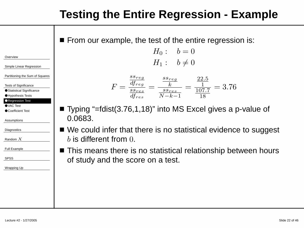
Testing the Entire Regression - Example
■ From our example, the test of the entire regression is:H0 : b = 0
H1 : b 6= 0
F =
ssreg
dfreg
ssres
dfres
=ssreg
kssres
N−k−1
=22.51
107.718
= 3.76
■ Typing “=fdist(3.76,1,18)” into MS Excel gives a p-value of0.0683.
■ We could infer that there is no statistical evidence to suggestb is different from 0.
■ This means there is no statistical relationship between hoursof study and the score on a test.

Overview
Simple Linear Regression
Partitioning the Sum of Squares
Tests of Significance
● Statistical Significance
● Hypothesis Tests
● Regression Test
● VAC Test
● Coefficient Test
Assumptions
Diagnostics
Random X
Full Example
SPSS
Wrapping Up
Lecture #2 - 1/27/2005 Slide 23 of 46
Testing the VAC
■ Because of the relationship of r2
xy with ssreg the previous testcould be phrased as:
F =
r2
xy
dfreg
1−r2xy
dfres
=
r2
xy
k
1−r2xy
N−k−1
=0.1728
1
1−0.172818
= 3.76
■ Notice this is identical to the F we received before.Therefore our conclusions are the same...

Overview
Simple Linear Regression
Partitioning the Sum of Squares
Tests of Significance
● Statistical Significance
● Hypothesis Tests
● Regression Test
● VAC Test
● Coefficient Test
Assumptions
Diagnostics
Random X
Full Example
SPSS
Wrapping Up
Lecture #2 - 1/27/2005 Slide 24 of 46
Testing the Regression Coefficient
■ Finally, the regression coefficient between X and Y cantested for difference from zero:
H0 : b = 0
H1 : b 6= 0
■ The variance of Y conditional on X is given by:
s2
y.x =
∑
(Y − Y ′)
N − k − 1=
ssres
N − k − 1
■ The standard error of the regression coefficient, sb, is basedon the conditional variance of Y |X:
sb =
√
s2y.x
∑
x2
Overview
Simple Linear Regression
Partitioning the Sum of Squares
Tests of Significance
● Statistical Significance
● Hypothesis Tests
● Regression Test
● VAC Test
● Coefficient Test
Assumptions
Diagnostics
Random X
Full Example
SPSS
Wrapping Up
Lecture #2 - 1/27/2005 Slide 25 of 46
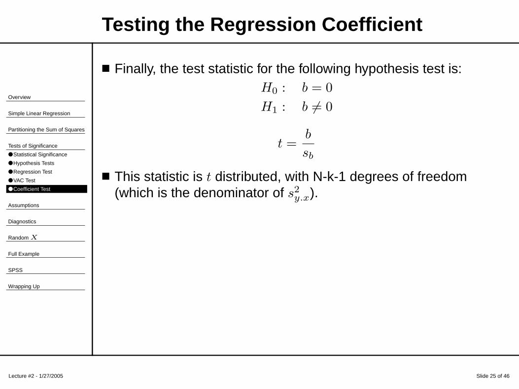
Testing the Regression Coefficient
■ Finally, the test statistic for the following hypothesis test is:H0 : b = 0
H1 : b 6= 0
t =b
sb
■ This statistic is t distributed, with N-k-1 degrees of freedom(which is the denominator of s2
y.x).

Overview
Simple Linear Regression
Partitioning the Sum of Squares
Tests of Significance
● Statistical Significance
● Hypothesis Tests
● Regression Test
● VAC Test
● Coefficient Test
Assumptions
Diagnostics
Random X
Full Example
SPSS
Wrapping Up
Lecture #2 - 1/27/2005 Slide 26 of 46
Testing the Regression Coefficient - Example
■ From our example, the test of the regression coefficient is:H0 : b = 0
H1 : b 6= 0
s2
y.x =
∑
(Y − Y ′)
N − k − 1=
ssres
N − k − 1=
107.7
18= 5.983
∑
x2 = 40
t =b
√
s2y.x
x2
=0.75
√
5.98340
= 1.94
■ Typing in “=tdist(1.94,18,2)” (2 for a two-tailed test), gives ap-value of 0.0683 - the same as before.
■ Recall F = t2 from somewhere before...

Overview
Simple Linear Regression
Partitioning the Sum of Squares
Tests of Significance
● Statistical Significance
● Hypothesis Tests
● Regression Test
● VAC Test
● Coefficient Test
Assumptions
Diagnostics
Random X
Full Example
SPSS
Wrapping Up
Lecture #2 - 1/27/2005 Slide 27 of 46
Testing the Regression Coefficient
■ In our example, we tested against zero.■ In reality, any value can be tested against:
H0 : b = B
H1 : b 6= B
t =b − B√
s2y.x
x2
Overview
Simple Linear Regression
Partitioning the Sum of Squares
Tests of Significance
Assumptions
● Assumptions
Diagnostics
Random X
Full Example
SPSS
Wrapping Up
Lecture #2 - 1/27/2005 Slide 28 of 46
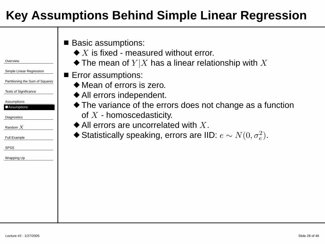
Key Assumptions Behind Simple Linear Regression
■ Basic assumptions:◆ X is fixed - measured without error.◆ The mean of Y |X has a linear relationship with X
■ Error assumptions:◆ Mean of errors is zero.◆ All errors independent.◆ The variance of the errors does not change as a function
of X - homoscedasticity.◆ All errors are uncorrelated with X.◆ Statistically speaking, errors are IID: e ∼ N(0, σ2
e).

Overview
Simple Linear Regression
Partitioning the Sum of Squares
Tests of Significance
Assumptions
Diagnostics
● Diagnostics
● Example
Random X
Full Example
SPSS
Wrapping Up
Lecture #2 - 1/27/2005 Slide 29 of 46
Diagnostics: Ways of Checking Assumptions
■ An easy way to check many error based assumptions avisualization:◆ A plot of the standardized residual versus the predicted
value.■ The next class will focus on other diagnostic measures.
Overview
Simple Linear Regression
Partitioning the Sum of Squares
Tests of Significance
Assumptions
Diagnostics
● Diagnostics
● Example
Random X
Full Example
SPSS
Wrapping Up
Lecture #2 - 1/27/2005 Slide 30 of 46
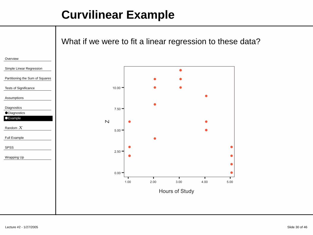
Curvilinear Example
What if we were to fit a linear regression to these data?
1.00 2.00 3.00 4.00 5.00
Hours of Study
0.00
2.50
5.00
7.50
10.00
Z
W
W
W
W
W
W
W
W
W
W
W
W
W
W
W
W
W
W
W
W

Overview
Simple Linear Regression
Partitioning the Sum of Squares
Tests of Significance
Assumptions
Diagnostics
● Diagnostics
● Example
Random X
Full Example
SPSS
Wrapping Up
Lecture #2 - 1/27/2005 Slide 31 of 46
Curvilinear Example
Fitting the simple linear regression model gives:
1.00 2.00 3.00 4.00 5.00
Hours of Study
0.00
2.50
5.00
7.50
10.00
Z
W
W
W
W
W
W
W
W
W
W
W
W
W
W
W
W
W
W
W
W
Z = 7.75 + −0.55 * X
R−Square = 0.04
Not good?

Overview
Simple Linear Regression
Partitioning the Sum of Squares
Tests of Significance
Assumptions
Diagnostics
● Diagnostics
● Example
Random X
Full Example
SPSS
Wrapping Up
Lecture #2 - 1/27/2005 Slide 32 of 46
Curvilinear Example
Let’s take a look at a plot of the standardized residuals versusthe predicted values:
5.00000 5.50000 6.00000 6.50000 7.00000
Unstandardized Predicted Value
−1.00000
0.00000
1.00000
Sta
nd
ard
ize
d R
esid
ua
l
W
W
W
W
W
W
W
W
W
W
W
W
W
W
W
W
W
W
W
W
Overview
Simple Linear Regression
Partitioning the Sum of Squares
Tests of Significance
Assumptions
Diagnostics
Random X
● Observational Studies
Full Example
SPSS
Wrapping Up
Lecture #2 - 1/27/2005 Slide 33 of 46
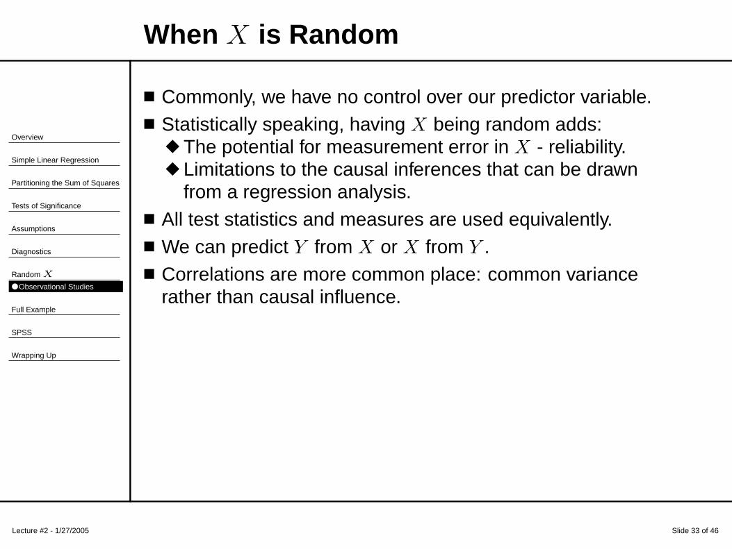
When X is Random
■ Commonly, we have no control over our predictor variable.■ Statistically speaking, having X being random adds:
◆ The potential for measurement error in X - reliability.◆ Limitations to the causal inferences that can be drawn
from a regression analysis.■ All test statistics and measures are used equivalently.■ We can predict Y from X or X from Y .■ Correlations are more common place: common variance
rather than causal influence.

Overview
Simple Linear Regression
Partitioning the Sum of Squares
Tests of Significance
Assumptions
Diagnostics
Random X
Full Example
● Old Faithful
● Scatterplot
● Descriptives
● Regression Line
● Hypothesis Tests
● Diagnostics
SPSS
Wrapping Up
Lecture #2 - 1/27/2005 Slide 34 of 46
Wrap Up Example
Example taken from Weisberg (1985, p. 230):
“Perhaps the most famous geyser is Old Faithful, inYellowstone National Park, Wyoming. The intervals oferuptions of Old Faithful range from about 30 to 90 minutes.Water shoots to heights generally over 35 meters, witheruptions lasting from 1 to 5.5 minutes.
“Data on Old Faithful has been collected for many years byranger/naturalists in the park, using a stopwatch. The durationmeasurements have been rounded to the nearest 0.1 minute or6 seconds, while intervals reported are to the nearest minute.The National Park Service uses x (values of the duration of aneruption) to predict y (the interval to the next eruption).”
Lecture #2 - 1/27/2005 Slide 35 of 46
Old Faithful Postcard

Overview
Simple Linear Regression
Partitioning the Sum of Squares
Tests of Significance
Assumptions
Diagnostics
Random X
Full Example
● Old Faithful
● Scatterplot
● Descriptives
● Regression Line
● Hypothesis Tests
● Diagnostics
SPSS
Wrapping Up
Lecture #2 - 1/27/2005 Slide 36 of 46
Old Faithful Scatterplot
1.00 2.00 3.00 4.00 5.00
Duration of Eruption
20.00
40.00
60.00
80.00
100.00
Inte
rva
l to
Ne
xt
Eru
ptio
nW
W
W
W
W
W
W
W
W
W
W
WW
W
W
W
W
W
W
W
W
W
W
W
W
W
W
WW
W
W
W
W
W
W
W
W
W
W
WW
W W
W
WWW
W
W
W
W
W
W
W
W
W
W
W
W
W
W
W
W
W
WW
W
W
WW
W
W
W
W
W
W
W
W
W
WW
W
W
W
W
W
W
WW
WW
W
W
W
W
WW
W
W
W
W
W
W
W
W
WW

Overview
Simple Linear Regression
Partitioning the Sum of Squares
Tests of Significance
Assumptions
Diagnostics
Random X
Full Example
● Old Faithful
● Scatterplot
● Descriptives
● Regression Line
● Hypothesis Tests
● Diagnostics
SPSS
Wrapping Up
Lecture #2 - 1/27/2005 Slide 37 of 46
Descriptive Statistics
Variable N Mean SD
x - Duration 107 3.4607 1.0363y - Interval 107 71.000 12.967
rxy = 0.858
r2
xy = 0.736∑
x2 = 113.84∑
y2 = 17, 822.00∑
xy = 1, 222.70

Overview
Simple Linear Regression
Partitioning the Sum of Squares
Tests of Significance
Assumptions
Diagnostics
Random X
Full Example
● Old Faithful
● Scatterplot
● Descriptives
● Regression Line
● Hypothesis Tests
● Diagnostics
SPSS
Wrapping Up
Lecture #2 - 1/27/2005 Slide 38 of 46
Regression Line
b =
∑
xy∑
x2=
1, 222.70
113.84= 10.74
a = Y − bX = 71.0 − (10.74) × 3.4607 = 33.84
Y ′ = 33.84 + 10.74X

Overview
Simple Linear Regression
Partitioning the Sum of Squares
Tests of Significance
Assumptions
Diagnostics
Random X
Full Example
● Old Faithful
● Scatterplot
● Descriptives
● Regression Line
● Hypothesis Tests
● Diagnostics
SPSS
Wrapping Up
Lecture #2 - 1/27/2005 Slide 39 of 46
Regression Line
2.00 3.00 4.00 5.00
Duration of Eruption
40.00
50.00
60.00
70.00
80.00
90.00
Inte
rva
l to
Ne
xt
Eru
ptio
nW
W
W
W
W
W
W
W
W
W
W
WW
W
W
W
W
W
W
W
W
W
W
W
W
W
W
WW
W
W
W
W
W
W
W
W
W
W
WW
W W
W
W
WW
W
W
W
W
W
W
W
W
W
W
W
W
W
W
W
W
W
WW
W
W
WW
W
W
W
W
W
W
W
W
W
WW
W
W
W
W
W
W
WW
W
W
W
W
W
W
W
W
W
W
W
W
W
W
W
W
WW
Interval to Next Eruption = 33.83 + 10.74 * X
R−Square = 0.74

Overview
Simple Linear Regression
Partitioning the Sum of Squares
Tests of Significance
Assumptions
Diagnostics
Random X
Full Example
● Old Faithful
● Scatterplot
● Descriptives
● Regression Line
● Hypothesis Tests
● Diagnostics
SPSS
Wrapping Up
Lecture #2 - 1/27/2005 Slide 40 of 46
Hypothesis Tests
ssreg = b∑
xy = 10.74 × 1, 222.70 = 13, 132.99
ssres =∑
y2 − ssreg = 17, 822.0 − 13, 132.99 = 4, 689.01
F =ssreg
kssres
N−k−1
=13, 132.99/1
4, 689.01/(107 − 1 − 1)= 294.084

Overview
Simple Linear Regression
Partitioning the Sum of Squares
Tests of Significance
Assumptions
Diagnostics
Random X
Full Example
● Old Faithful
● Scatterplot
● Descriptives
● Regression Line
● Hypothesis Tests
● Diagnostics
SPSS
Wrapping Up
Lecture #2 - 1/27/2005 Slide 41 of 46
Residual Plot
60.00000 70.00000 80.00000
Unstandardized Predicted Value
−2.00000
−1.00000
0.00000
1.00000
2.00000
Sta
nd
ard
ize
d R
esid
ua
l
WW
W
W
W
W
W
W
W
W
W
W
W
W
W W
W
W
W
W
W
W
W
W W
W
W
W
W
W
W
W
W
W
W
WW
W
W
WW
W
W
W
W
WW
W
W
W
W
W
W
W
W
W
W
W
W
W
W
W
W
W
WW
W
W
W
W
W
W
W
W
W
W
WW
W W
W
W
W
W
W
W
W
W
WW
W
W
W
W
W
WW
W
W
W
W
W
W
W
WW
W

Overview
Simple Linear Regression
Partitioning the Sum of Squares
Tests of Significance
Assumptions
Diagnostics
Random X
Full Example
SPSS
● Data
● More Data
● Scatterplots
Wrapping Up
Lecture #2 - 1/27/2005 Slide 42 of 46
Data

Overview
Simple Linear Regression
Partitioning the Sum of Squares
Tests of Significance
Assumptions
Diagnostics
Random X
Full Example
SPSS
● Data
● More Data
● Scatterplots
Wrapping Up
Lecture #2 - 1/27/2005 Slide 43 of 46
Data

Overview
Simple Linear Regression
Partitioning the Sum of Squares
Tests of Significance
Assumptions
Diagnostics
Random X
Full Example
SPSS
● Data
● More Data
● Scatterplots
Wrapping Up
Lecture #2 - 1/27/2005 Slide 44 of 46
Plots from Today
Scatterplots were made with the interactive graphs:Graphs...Interactive...Scatterplot.

Overview
Simple Linear Regression
Partitioning the Sum of Squares
Tests of Significance
Assumptions
Diagnostics
Random X
Full Example
SPSS
● Data
● More Data
● Scatterplots
Wrapping Up
Lecture #2 - 1/27/2005 Slide 45 of 46
Simple Linear Regression
Analyze...Regression...Linear.

Overview
Simple Linear Regression
Partitioning the Sum of Squares
Tests of Significance
Assumptions
Diagnostics
Random X
Full Example
SPSS
● Data
● More Data
● Scatterplots
Wrapping Up
Lecture #2 - 1/27/2005 Slide 46 of 46
Saving Residuals
Analyze...Regression...Linear → Save Button.
Overview
Simple Linear Regression
Partitioning the Sum of Squares
Tests of Significance
Assumptions
Diagnostics
Random X
Full Example
SPSS
Wrapping Up
● Final Thought
● Next Class
Lecture #2 - 1/27/2005 Slide 47 of 46
Final Thought
■ Simple linear regressioncan be simple and straightforward.
■ Need to understanddifference betweenstatistical significance andpractical relevance.
■ The tests of significance and model estimates are only validif all assumptions are met.
■ Regression is fairly robust to violations of assumptions, but...■ Usually when assumptions are violated, something else is
wrong with the model.■ Listen to your data, they are trying to tell you something.

Overview
Simple Linear Regression
Partitioning the Sum of Squares
Tests of Significance
Assumptions
Diagnostics
Random X
Full Example
SPSS
Wrapping Up
● Final Thought
● Next Class
Lecture #2 - 1/27/2005 Slide 48 of 46
Next Time
■ Regression diagnostics - Chapter 3.■ More SPSS.■ More practice with fitting models.■ QUESTION: Do you have any data you are willing to share
with class?