Applied Quantitative Analysis and Practices

LECTURE#22

By

Dr. Osman Sadiq Paracha

Previous Lecture Summary Application in SPSS for factor analysis stages Interpretation of factor matrix Validation of factor analysis Factor Scores

Simple Linear Regression

Correlation vs. Regression

A scatter plot can be used to show the relationship between two variables

Correlation analysis is used to measure the strength of the association (linear relationship) between two variables Correlation is only concerned with strength of the

relationship No causal effect is implied with correlation

DCOVA

Types of Relationships

Y

X

Y

X

Y

Y

X

X

Linear relationships Curvilinear relationships

DCOVA

Types of Relationships

Y

X

Y

X

Y

Y

X

X

Strong relationships Weak relationships

(continued)

DCOVA

Types of Relationships

Y

X

Y

X

No relationship

(continued)DCOVA

Introduction to Regression Analysis

Regression analysis is used to: Predict the value of a dependent variable based on

the value of at least one independent variable Explain the impact of changes in an independent

variable on the dependent variable

Dependent variable: the variable we wish to predict or explain

Independent variable: the variable used to predict or explain the

dependent variable

DCOVA

Simple Linear Regression Model

Only one independent variable, X Relationship between X and Y is

described by a linear function Changes in Y are assumed to be related

to changes in X

DCOVA

ii10i εXββY Linear component

Simple Linear Regression Model

Population Y intercept

Population SlopeCoefficient

Random Error term

Dependent Variable

Independent Variable

Random Error component

DCOVA

(continued)

Random Error for this Xi value

Y

X

Observed Value of Y for Xi

Predicted Value of Y for Xi

ii10i εXββY

Xi

Slope = β1

Intercept = β0

εi

Simple Linear Regression Model DCOVA

i10i XbbY

The simple linear regression equation provides an estimate of the population regression line

Simple Linear Regression Equation (Prediction Line)

Estimate of the regression

intercept

Estimate of the regression slope

Estimated (or predicted) Y value for observation i

Value of X for observation i

DCOVA

The Least Squares Method

b0 and b1 are obtained by finding the values of

that minimize the sum of the squared

differences between Y and :

2i10i

2ii ))Xb(b(Ymin)Y(Ymin

Y

Finding the Least Squares Equation

The coefficients b0 and b1 , can be found through the below mentioned formula

b1 =

b0 =

b0 is the estimated average value of Y

when the value of X is zero

b1 is the estimated change in the

average value of Y as a result of a one-unit increase in X

Interpretation of the Slope and the Intercept

Simple Linear Regression Example

A real estate agent wishes to examine the relationship between the selling price of a home and its size (measured in square feet)

A random sample of 10 houses is selected Dependent variable (Y) = house price in $1000s Independent variable (X) = square feet

Simple Linear Regression Example: Data

House Price in $1000s(Y)

Square Feet (X)

245 1400

312 1600

279 1700

308 1875

199 1100

219 1550

405 2350

324 2450

319 1425

255 1700

0

50

100

150

200

250

300

350

400

450

0 500 1000 1500 2000 2500 3000

Ho

use

Pri

ce ($

1000

s)

Square Feet

Simple Linear Regression Example: Scatter Plot

House price model: Scatter Plot

Simple Linear Regression ExampleRegression Statistics

Multiple R 0.76211

R Square 0.58082

Adjusted R Square 0.52842

Standard Error 41.33032

Observations 10

ANOVA  df SS MS F Significance F

Regression 1 18934.9348 18934.9348 11.0848 0.01039

Residual 8 13665.5652 1708.1957

Total 9 32600.5000      

  Coefficients Standard Error t Stat P-value Lower 95% Upper 95%

Intercept 98.24833 58.03348 1.69296 0.12892 -35.57720 232.07386

Square Feet 0.10977 0.03297 3.32938 0.01039 0.03374 0.18580

The regression equation is:

feet) (square 0.10977 98.24833 price house

0

50

100

150

200

250

300

350

400

450

0 500 1000 1500 2000 2500 3000

Square Feet

Ho

use

Pri

ce (

$100

0s)

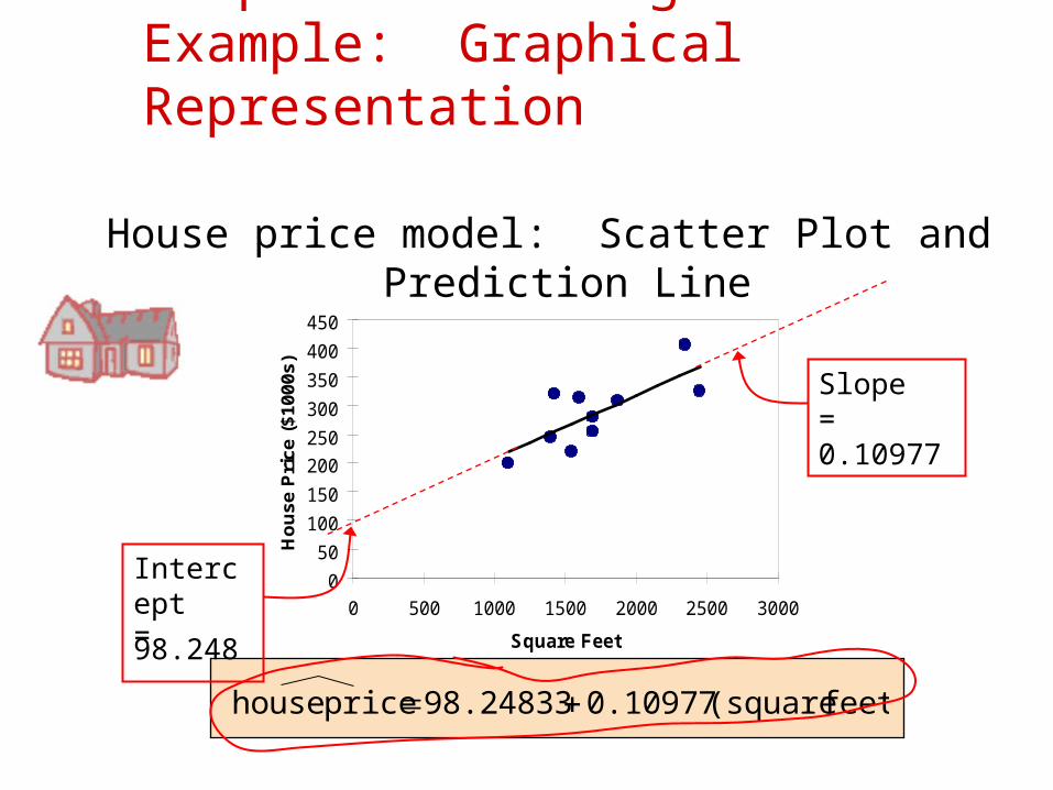
Simple Linear Regression Example: Graphical Representation

House price model: Scatter Plot and Prediction Line

feet) (square 0.10977 98.24833 price house

Slope = 0.10977

Intercept = 98.248

Simple Linear Regression Example: Interpretation of bo

b0 is the estimated average value of Y when the

value of X is zero (if X = 0 is in the range of observed X values)

Because a house cannot have a square footage of 0, b0 has no practical application

feet) (square 0.10977 98.24833 price house

Simple Linear Regression Example: Interpreting b1

b1 estimates the change in the average

value of Y as a result of a one-unit increase in X Here, b1 = 0.10977 tells us that the mean value of a

house increases by .10977($1000) = $109.77, on average, for each additional one square foot of size

feet) (square 0.10977 98.24833 price house

317.85

0)0.1098(200 98.25

(sq.ft.) 0.1098 98.25 price house

Predict the price for a house with 2000 square feet:

The predicted price for a house with 2000 square feet is 317.85($1,000s) = $317,850

Simple Linear Regression Example: Making Predictions

0

50

100

150

200

250

300

350

400

450

0 500 1000 1500 2000 2500 3000

Square Feet

Ho

use

Pri

ce (

$100

0s)

Simple Linear Regression Example: Making Predictions

When using a regression model for prediction, only predict within the relevant range of data

Relevant range for interpolation

Do not try to extrapolate

beyond the range of observed X’s

Measures of Variation

Total variation is made up of two parts:

SSE SSR SST Total Sum of

SquaresRegression Sum

of SquaresError Sum of

Squares

2i )YY(SST 2

ii )YY(SSE 2i )YY(SSR

where:

= Mean value of the dependent variable

Yi = Observed value of the dependent variable

= Predicted value of Y for the given Xi valueiY

Y

SST = total sum of squares (Total Variation)

Measures the variation of the Yi values around their mean Y

SSR = regression sum of squares (Explained Variation) Variation attributable to the relationship between X

and Y SSE = error sum of squares (Unexplained Variation)

Variation in Y attributable to factors other than X

(continued)

Measures of Variation

Lecture Summary Simple Linear Regression Correlation Vs Regression Introduction to Simple Linear Regression Simple Linear Regression Model Least Square Method Interpretation of Model Measures of variation