applied probability and stochastic processes
DESCRIPTION
Applied Probability and Stochastic Processes (Lecture Notes)TRANSCRIPT
AppliedProbability and Stochastic Processes
Lecture Notes for 577/578 Class
W lodzimierz Bryc
Department of Mathematics
University of Cincinnati
P. O. Box 210025
Cincinnati, OH 45221-0025
E-mail: [email protected]
Created: October 22, 1995
Printed: March 21, 1996
c 1995 W lodzimierz Bryc
Cincinnati Free Texts

Contents
I Probability 3
1 Random phenomena 11.1 Mathematical models, and stochastic models : : : : : : : : : : : : : : : : : 11.2 Events and their chances : : : : : : : : : : : : : : : : : : : : : : : : : : : : 2
1.2.1 Uniform Probability : : : : : : : : : : : : : : : : : : : : : : : : : : 31.2.2 Geometric Probability : : : : : : : : : : : : : : : : : : : : : : : : : 5
1.3 Elementary probability models : : : : : : : : : : : : : : : : : : : : : : : : : 51.3.1 Consequences of axioms : : : : : : : : : : : : : : : : : : : : : : : : 51.3.2 General discrete sample space : : : : : : : : : : : : : : : : : : : : : 61.3.3 General continuous sample space : : : : : : : : : : : : : : : : : : : 6
1.4 Simulating discrete events : : : : : : : : : : : : : : : : : : : : : : : : : : : 71.4.1 Generic simulation template : : : : : : : : : : : : : : : : : : : : : : 81.4.2 Blind search : : : : : : : : : : : : : : : : : : : : : : : : : : : : : : : 91.4.3 Application: Traveling salesman problem : : : : : : : : : : : : : : : 101.4.4 Improving blind search : : : : : : : : : : : : : : : : : : : : : : : : : 121.4.5 Random permutations : : : : : : : : : : : : : : : : : : : : : : : : : 13
1.5 Conditional probability : : : : : : : : : : : : : : : : : : : : : : : : : : : : : 141.5.1 Properties of conditional probability : : : : : : : : : : : : : : : : : 141.5.2 Sequential experiments : : : : : : : : : : : : : : : : : : : : : : : : : 15
1.6 Independent events : : : : : : : : : : : : : : : : : : : : : : : : : : : : : : : 161.6.1 Random variables : : : : : : : : : : : : : : : : : : : : : : : : : : : : 171.6.2 Binomial trials : : : : : : : : : : : : : : : : : : : : : : : : : : : : : 17
1.7 Further notes about simulations : : : : : : : : : : : : : : : : : : : : : : : : 191.8 Questions : : : : : : : : : : : : : : : : : : : : : : : : : : : : : : : : : : : : 19
2 Random variables (continued) 212.1 Discrete r. v. : : : : : : : : : : : : : : : : : : : : : : : : : : : : : : : : : : 21
2.1.1 Examples of discrete r. v. : : : : : : : : : : : : : : : : : : : : : : : 222.1.2 Simulations of discrete r. v. : : : : : : : : : : : : : : : : : : : : : : 22
2.2 Continuous r. v. : : : : : : : : : : : : : : : : : : : : : : : : : : : : : : : : : 232.2.1 Examples of continuous r. v. : : : : : : : : : : : : : : : : : : : : : : 232.2.2 Histograms : : : : : : : : : : : : : : : : : : : : : : : : : : : : : : : 242.2.3 Simulations of continuous r. v. : : : : : : : : : : : : : : : : : : : : : 24
2.3 Expected values : : : : : : : : : : : : : : : : : : : : : : : : : : : : : : : : : 252.3.1 Tail integration formulas : : : : : : : : : : : : : : : : : : : : : : : : 262.3.2 Chebyshev-Markov inequality : : : : : : : : : : : : : : : : : : : : : 27
iii

iv CONTENTS
2.4 Expected values and simulations : : : : : : : : : : : : : : : : : : : : : : : : 282.5 Joint distributions : : : : : : : : : : : : : : : : : : : : : : : : : : : : : : : 30
2.5.1 Independent random variables : : : : : : : : : : : : : : : : : : : : : 312.6 Functions of r. v. : : : : : : : : : : : : : : : : : : : : : : : : : : : : : : : : 312.7 Moments of functions : : : : : : : : : : : : : : : : : : : : : : : : : : : : : : 32
2.7.1 Simulations : : : : : : : : : : : : : : : : : : : : : : : : : : : : : : : 342.8 Application: scheduling : : : : : : : : : : : : : : : : : : : : : : : : : : : : : 34
2.8.1 Deterministic scheduling problem : : : : : : : : : : : : : : : : : : : 342.8.2 Stochastic scheduling problem : : : : : : : : : : : : : : : : : : : : : 352.8.3 More scheduling questions : : : : : : : : : : : : : : : : : : : : : : : 35
2.9 Distributions of functions : : : : : : : : : : : : : : : : : : : : : : : : : : : : 352.10 L2-spaces : : : : : : : : : : : : : : : : : : : : : : : : : : : : : : : : : : : : 372.11 Correlation coe�cient : : : : : : : : : : : : : : : : : : : : : : : : : : : : : 38
2.11.1 Best linear approximation : : : : : : : : : : : : : : : : : : : : : : : 382.12 Application: length of a random chain : : : : : : : : : : : : : : : : : : : : 392.13 Conditional expectations : : : : : : : : : : : : : : : : : : : : : : : : : : : : 39
2.13.1 Conditional distributions : : : : : : : : : : : : : : : : : : : : : : : : 392.13.2 Conditional expectations as random variables : : : : : : : : : : : : 402.13.3 Conditional expectations (continued) : : : : : : : : : : : : : : : : : 40
2.14 Best non-linear approximations : : : : : : : : : : : : : : : : : : : : : : : : 412.15 Lack of memory : : : : : : : : : : : : : : : : : : : : : : : : : : : : : : : : : 412.16 Intensity of failures : : : : : : : : : : : : : : : : : : : : : : : : : : : : : : : 422.17 Poisson approximation : : : : : : : : : : : : : : : : : : : : : : : : : : : : : 422.18 Questions : : : : : : : : : : : : : : : : : : : : : : : : : : : : : : : : : : : : 43
3 Moment generating functions 453.1 Generating functions : : : : : : : : : : : : : : : : : : : : : : : : : : : : : : 453.2 Properties : : : : : : : : : : : : : : : : : : : : : : : : : : : : : : : : : : : : 45
3.2.1 Probability generating functions : : : : : : : : : : : : : : : : : : : : 473.3 Characteristic functions : : : : : : : : : : : : : : : : : : : : : : : : : : : : 473.4 Questions : : : : : : : : : : : : : : : : : : : : : : : : : : : : : : : : : : : : 47
4 Normal distribution 494.1 Herschel's law of errors : : : : : : : : : : : : : : : : : : : : : : : : : : : : : 504.2 Bivariate Normal distribution : : : : : : : : : : : : : : : : : : : : : : : : : 524.3 Questions : : : : : : : : : : : : : : : : : : : : : : : : : : : : : : : : : : : : 52
5 Limit theorems 535.1 Stochastic Analysis : : : : : : : : : : : : : : : : : : : : : : : : : : : : : : : 535.2 Law of large numbers : : : : : : : : : : : : : : : : : : : : : : : : : : : : : : 53
5.2.1 Strong law of large numbers : : : : : : : : : : : : : : : : : : : : : : 545.3 Convergence of distributions : : : : : : : : : : : : : : : : : : : : : : : : : : 545.4 Central Limit Theorem : : : : : : : : : : : : : : : : : : : : : : : : : : : : : 555.5 Limit theorems and simulations : : : : : : : : : : : : : : : : : : : : : : : : 575.6 Large deviation bounds : : : : : : : : : : : : : : : : : : : : : : : : : : : : : 575.7 Conditional limit theorems : : : : : : : : : : : : : : : : : : : : : : : : : : : 58

CONTENTS v
5.8 Questions : : : : : : : : : : : : : : : : : : : : : : : : : : : : : : : : : : : : 58
II Stochastic processes 59
6 Simulations 616.1 Generating random numbers : : : : : : : : : : : : : : : : : : : : : : : : : : 61
6.1.1 Random digits : : : : : : : : : : : : : : : : : : : : : : : : : : : : : 616.1.2 Overview of random number generators : : : : : : : : : : : : : : : : 62
6.2 Simulating discrete r. v. : : : : : : : : : : : : : : : : : : : : : : : : : : : : 636.2.1 Generic Method { discrete case : : : : : : : : : : : : : : : : : : : : 636.2.2 Geometric : : : : : : : : : : : : : : : : : : : : : : : : : : : : : : : : 636.2.3 Binomial : : : : : : : : : : : : : : : : : : : : : : : : : : : : : : : : : 636.2.4 Poisson : : : : : : : : : : : : : : : : : : : : : : : : : : : : : : : : : 63
6.3 Simulating continuous r. v. : : : : : : : : : : : : : : : : : : : : : : : : : : : 636.3.1 Generic Method { continuous case : : : : : : : : : : : : : : : : : : : 636.3.2 Randomization : : : : : : : : : : : : : : : : : : : : : : : : : : : : : 646.3.3 Simulating normal distribution : : : : : : : : : : : : : : : : : : : : 64
6.4 Rejection sampling : : : : : : : : : : : : : : : : : : : : : : : : : : : : : : : 646.5 Simulating discrete experiments : : : : : : : : : : : : : : : : : : : : : : : : 65
6.5.1 Random subsets : : : : : : : : : : : : : : : : : : : : : : : : : : : : : 656.5.2 Random Permutations : : : : : : : : : : : : : : : : : : : : : : : : : 65
6.6 Integration by simulations : : : : : : : : : : : : : : : : : : : : : : : : : : : 666.6.1 Strati�ed sampling : : : : : : : : : : : : : : : : : : : : : : : : : : : 66
6.7 Monte Carlo estimation of small probabilities : : : : : : : : : : : : : : : : 66
7 Introduction to stochastic processes 697.1 Di�erence Equations : : : : : : : : : : : : : : : : : : : : : : : : : : : : : : 69
7.1.1 Examples : : : : : : : : : : : : : : : : : : : : : : : : : : : : : : : : 697.2 Linear di�erence equations : : : : : : : : : : : : : : : : : : : : : : : : : : : 71
7.2.1 Problems : : : : : : : : : : : : : : : : : : : : : : : : : : : : : : : : 737.3 Recursive equations, chaos, randomness : : : : : : : : : : : : : : : : : : : : 747.4 Modeling and simulation : : : : : : : : : : : : : : : : : : : : : : : : : : : : 767.5 Random walks : : : : : : : : : : : : : : : : : : : : : : : : : : : : : : : : : : 77
7.5.1 Stopping times : : : : : : : : : : : : : : : : : : : : : : : : : : : : : 777.5.2 Example: chromatography : : : : : : : : : : : : : : : : : : : : : : : 787.5.3 Ruining a gambler : : : : : : : : : : : : : : : : : : : : : : : : : : : 787.5.4 Random growth model : : : : : : : : : : : : : : : : : : : : : : : : : 78
8 Markov processes 818.1 Markov chains : : : : : : : : : : : : : : : : : : : : : : : : : : : : : : : : : : 81
8.1.1 Finite state space : : : : : : : : : : : : : : : : : : : : : : : : : : : : 828.1.2 Markov processes and graphs : : : : : : : : : : : : : : : : : : : : : 83
8.2 Simulating Markov chains : : : : : : : : : : : : : : : : : : : : : : : : : : : 858.2.1 Example: soccer : : : : : : : : : : : : : : : : : : : : : : : : : : : : : 85
8.3 One step analysis : : : : : : : : : : : : : : : : : : : : : : : : : : : : : : : : 868.3.1 Example: vehicle insurance claims : : : : : : : : : : : : : : : : : : : 87
vi CONTENTS
8.3.2 Example: a game of piggy : : : : : : : : : : : : : : : : : : : : : : : 878.4 Recurrence : : : : : : : : : : : : : : : : : : : : : : : : : : : : : : : : : : : : 898.5 Simulated annealing : : : : : : : : : : : : : : : : : : : : : : : : : : : : : : 89
8.5.1 Program listing : : : : : : : : : : : : : : : : : : : : : : : : : : : : : 908.6 Solving di�erence equations through simulations : : : : : : : : : : : : : : : 908.7 Markov Autoregressive processes : : : : : : : : : : : : : : : : : : : : : : : : 908.8 Sorting at random : : : : : : : : : : : : : : : : : : : : : : : : : : : : : : : 918.9 An application: �nd k-th largest number : : : : : : : : : : : : : : : : : : : 92
9 Branching processes 939.1 The mean and the variance : : : : : : : : : : : : : : : : : : : : : : : : : : 939.2 Generating functions of Branching processes : : : : : : : : : : : : : : : : : 93
9.2.1 Extinction : : : : : : : : : : : : : : : : : : : : : : : : : : : : : : : : 949.3 Two-valued case : : : : : : : : : : : : : : : : : : : : : : : : : : : : : : : : : 949.4 Geometric case : : : : : : : : : : : : : : : : : : : : : : : : : : : : : : : : : 94
10 Multivariate normal distribution 9710.1 Multivariate moment generating function : : : : : : : : : : : : : : : : : : : 9710.2 Bivariate normal distribution : : : : : : : : : : : : : : : : : : : : : : : : : 98
10.2.1 Example: normal random walk : : : : : : : : : : : : : : : : : : : : 9910.3 Simulating a multivariate normal distribution : : : : : : : : : : : : : : : : 100
10.3.1 General multivariate normal law : : : : : : : : : : : : : : : : : : : : 10010.4 Covariance matrix : : : : : : : : : : : : : : : : : : : : : : : : : : : : : : : 100
10.4.1 Multivariate normal density : : : : : : : : : : : : : : : : : : : : : : 10110.4.2 Linear regression : : : : : : : : : : : : : : : : : : : : : : : : : : : : 101
10.5 Gaussian Markov processes : : : : : : : : : : : : : : : : : : : : : : : : : : : 102
11 Continuous time processes 10311.1 Poisson process : : : : : : : : : : : : : : : : : : : : : : : : : : : : : : : : : 103
11.1.1 The law of rare events : : : : : : : : : : : : : : : : : : : : : : : : : 10511.1.2 Compound Poisson process : : : : : : : : : : : : : : : : : : : : : : : 105
11.2 Continuous time Markov processes : : : : : : : : : : : : : : : : : : : : : : 10611.2.1 Examples of continuous time Markov processes : : : : : : : : : : : 107
11.3 Gaussian processes : : : : : : : : : : : : : : : : : : : : : : : : : : : : : : : 10811.4 The Wiener process : : : : : : : : : : : : : : : : : : : : : : : : : : : : : : : 108
12 Time Series 10912.1 Second order stationary processes : : : : : : : : : : : : : : : : : : : : : : : 109
12.1.1 Positive de�nite functions : : : : : : : : : : : : : : : : : : : : : : : 11012.2 Trajectory averages : : : : : : : : : : : : : : : : : : : : : : : : : : : : : : : 11012.3 The general prediction problem : : : : : : : : : : : : : : : : : : : : : : : : 11012.4 Autoregressive processes : : : : : : : : : : : : : : : : : : : : : : : : : : : : 111
13 Additional topics 11313.1 A simple probabilistic modeling in Genetics : : : : : : : : : : : : : : : : : 11313.2 Application: verifying matrix multiplication : : : : : : : : : : : : : : : : : 11413.3 Exchangeability : : : : : : : : : : : : : : : : : : : : : : : : : : : : : : : : : 114

CONTENTS vii
13.4 Distances between strings : : : : : : : : : : : : : : : : : : : : : : : : : : : 11613.5 A model of cell growth : : : : : : : : : : : : : : : : : : : : : : : : : : : : : 11813.6 Shannon's Entropy : : : : : : : : : : : : : : : : : : : : : : : : : : : : : : : 118
13.6.1 Optimal search : : : : : : : : : : : : : : : : : : : : : : : : : : : : : 11813.7 Application: spread of epidemic : : : : : : : : : : : : : : : : : : : : : : : : 119
A Theoretical complements 121A.1 Lp-spaces : : : : : : : : : : : : : : : : : : : : : : : : : : : : : : : : : : : : 121A.2 Properties of conditional expectations : : : : : : : : : : : : : : : : : : : : : 122
B Math background 125B.1 Interactive links : : : : : : : : : : : : : : : : : : : : : : : : : : : : : : : : : 125B.2 Elementary combinatorics : : : : : : : : : : : : : : : : : : : : : : : : : : : 125B.3 Limits : : : : : : : : : : : : : : : : : : : : : : : : : : : : : : : : : : : : : : 125B.4 Power series expansions : : : : : : : : : : : : : : : : : : : : : : : : : : : : : 126B.5 Multivariate integration : : : : : : : : : : : : : : : : : : : : : : : : : : : : 126B.6 Di�erential equations : : : : : : : : : : : : : : : : : : : : : : : : : : : : : : 126B.7 Linear algebra : : : : : : : : : : : : : : : : : : : : : : : : : : : : : : : : : : 126B.8 Fourier series : : : : : : : : : : : : : : : : : : : : : : : : : : : : : : : : : : 127B.9 Powers of matrices : : : : : : : : : : : : : : : : : : : : : : : : : : : : : : : 127
C Numerical Methods 129C.1 Numerical integration : : : : : : : : : : : : : : : : : : : : : : : : : : : : : : 129C.2 Solving equations : : : : : : : : : : : : : : : : : : : : : : : : : : : : : : : : 129C.3 Searching for minimum : : : : : : : : : : : : : : : : : : : : : : : : : : : : : 129
D Programming Help 131D.1 Introducing BASIC : : : : : : : : : : : : : : : : : : : : : : : : : : : : : : : 131D.2 Computing : : : : : : : : : : : : : : : : : : : : : : : : : : : : : : : : : : : 131D.3 The structure of a program : : : : : : : : : : : : : : : : : : : : : : : : : : 132D.4 Conditionals and loops : : : : : : : : : : : : : : : : : : : : : : : : : : : : : 133D.5 User input : : : : : : : : : : : : : : : : : : : : : : : : : : : : : : : : : : : : 134D.6 More about printing : : : : : : : : : : : : : : : : : : : : : : : : : : : : : : 134D.7 Arrays and matrices : : : : : : : : : : : : : : : : : : : : : : : : : : : : : : 135D.8 Data types : : : : : : : : : : : : : : : : : : : : : : : : : : : : : : : : : : : : 135D.9 User de�ned FUNCTIONs and SUBs : : : : : : : : : : : : : : : : : : : : : 135D.10 Graphics : : : : : : : : : : : : : : : : : : : : : : : : : : : : : : : : : : : : : 136D.11 Binary operations : : : : : : : : : : : : : : : : : : : : : : : : : : : : : : : : 136D.12 File Operations : : : : : : : : : : : : : : : : : : : : : : : : : : : : : : : : : 136D.13 Good programming : : : : : : : : : : : : : : : : : : : : : : : : : : : : : : : 137D.14 Example: designing an automatic card dealer : : : : : : : : : : : : : : : : 137
D.14.1 First Iteration : : : : : : : : : : : : : : : : : : : : : : : : : : : : : : 138D.14.2 Second Iteration : : : : : : : : : : : : : : : : : : : : : : : : : : : : 139D.14.3 Third iteration : : : : : : : : : : : : : : : : : : : : : : : : : : : : : 140
Bibliography 144

viii Description
Course description
This course is aimed at students in applied �elds and assumes a prerequisite of calculus.The goal is a working knowledge of the concepts and uses of modern probability theory.A signi�cant part of such a \working knowledge" in modern applications of mathematicsis computer-dependent.
The course contains mathematical problems and computer exercises. Students will beexpected to write and execute programs pertinent to the material of the course. No pro-gramming experience is necessary or assumed. But the willingness to accept a computeras a tool is a requirement.
For novices, BASIC programming language, (QBASIC in DOS,Visual Basic inWin-dows, or BASIC on Macintosh) is recommended. BASIC is perhaps the easiest program-ming language to learn, and the �rst programming language is always the hardest topick.
Programs in QBASIC 4.5 on IBM-compatible PC and, to a lesser extend, programson Texas Instrument Programmable calculator TI-85, and WindowsTM programs inMicrosoft Visual Basic 3.0 are supported. This means that I will attempt to an-swer technical questions and provide examples. Other programming languages (SAS, C,
C++, Fortran, Cobol, Assembler, Mathematica, LISP, TEX(!), Excel, etc.) canbe used, but I will not be able to help with the technical issues.
Contents of the course (subject to change)
577 Basic elements of probability. Poisson, geometric, binomial, normal, exponentialdistributions. Simulations. Conditioning, characterizations.
Moment generating functions, limit theorems, characteristic functions. Stochasticprocesses: random walks, Markov sequences, the Poisson process.
578 Time dependent and stochastic processes: Markov processes, branching processes.Modeling
Multivariate normal distribution. Gaussian processes, white noise. Conditionalexpectations. Fourier expansions, time series.
Supporting materials
This text is available through Internet1 in PostScript, or DVI. A number of other mathrelated resources can be found on WWW2. Also available are supporting BASIC3 program�les. Support for Pascal is anticipated in the future.
Auxiliary textbooks:
� W. Feller, An Introduction to Probability Theory, Vol. I, Wiley 1967. Vol II, Wiley,New York 1966
1http://math.uc.edu/~brycw/probab/books/2http://archives.math.utk.edu/tutorials.html3http://math.uc.edu/~brycw/probab/basic.htm

Description ix
Volume I is an excellent introduction to elementary and not-that-elementary prob-ability. Volume II is advanced.
� W. H. Press, S. A. Teukolsky, W. T. Vetterling, B. P. Flannery, Numerical recipesin C, Cambridge University Press, New YorkA reference for numerical methods: C-language version.
� J. C. Sprott Numerical recipes Routines and Examples in BASIC, Cambridge Uni-versity Press, New York 1992A reference for numerical methods: routines in QuickBasic 4.5 version.
� H. M. Taylor & S. Karlin, An introduction to stochastic modeling, Acad. Press,Boston 1984Markov chains with many examples/models, Branching processes, Queueing sys-tems.
� L. Breiman, Probability and Stochastic Processes: with a view towards applications,Houghton Mi�in, Boston 1969.includes Markov chains and spectral theory of stationary processes.
� R. E. Barlow & F. Proschan, Mathematical Theory of Reliability, SIAM series inapplied math, Wiley, New York 1965.Advanced compendium of reliability theory methods (mid-sixties).
� S. Biswas, Applied Stochastic Processes, Wiley, New York 1995Techniques of interest in population dynamics, epidemiology, clinical drug trials,fertility and mortality analysis.
� J. Higgins & S. Keller-McNulty, Concepts in Probability and Stochastic ModelingDuxbury Press 1995Covers traditional material; computer simulations complement theory.
� T. Harris, The Theory of Branching Processes Reprinted: Dover, 1989.A classic on Branching processes.
� H. C. Tjims, Stochastic models. An algorithmic approach, Wiley, Chichester, 1994.Renewal processes, reliability, inventory models, queuieing models.
Conventions
Exercises
The text has three types of \practice questions", marked as Problems, Exercises, andProjects. Examples vary the most and could be solved in class by an instructor; Exercisesare intended primarily for computer-assisted analysis; Problems are of more mathematicalnature. Projects are longer, and frequently open-ended. Exercises, Projects, and Problemsare numbered consecutively within chapters; for instance Exercise 10.2 follows Problem10.1, meaning that there is no Exercise 10.1.

x Description
Programming
The text refers to BASIC instructions with the convention that BASIC key-words are cap-italized, the names of variables, functions, and the SUBs are mixed case like ThisExample.Program listings are typeset in a special \computer" font to distinguish them from therest of the text.

License 1
Copyright and License for 1996 version
This textbook is copyrighted c W. Bryc 1996. All rights re-served. GTDR.
Academic users are granted the right to make copies for theirpersonal use, and for distribution to their students in academicyear 1995/1996.
Reproduction in any form by commercial publishers, includingtextbook publishers, requires written permission from the copy-right holder.
Cincinnati Free Texts c 1996 W. Bryc

2 License

Part I
Probability
3


Chapter 1
Random phenomena
De�nition of a Tree: A tree is a woody plant with erect perennial trunk of atleast 3.5 inches (7.5 centimeters) in diameter at breast height (41
2feet or 1.3
meters), a de�nitely formed crown of foliage, and a height of at least 13 feet(4 meters).The Auborn Society Field Guide to North American Trees.
This chapter introduces fundamental concepts of probability theory; events, and theirchances. For the readers who are familiar with elementary probability it may be refreshingto see the computer used for counting elementary events, and randomization used to solvea deterministic optimization problem.
The questions are
� What is \probability"?
� How do we evaluate probabilities in real-life situations?
� What is the computer good for?
1.1 Mathematical models, and stochastic models
Every theory has its successes, and its limitations. These notes are about the successesof probability theory. But it doesn't hurt to explain in non-technical language some ofits limitations up front. This way the reader can understand the basic premise beforeinvesting considerable time.
To begin with, we start with a truism. Real world is complicated, often to a largerdegree than scientists will readily admit. Most real phenomena have multi-aspect form,and can be approached in multiple ways. Various questions can be asked. Even seeminglythe same question can be answered on many incompatible levels. For instance, the genericquestion about dinosaur extinction has the following variants.
� Why did Dino the dinosaur die? Was she bitten by a poisonous rat-like creature?Hit by a meteorite? Froze to death?
� Why did the crocodiles survive to our times, and tyranosaurus rex didn't?
1
2 CHAPTER 1. RANDOM PHENOMENA
� What was the cause of the dinosaur extinction?
� Was the dinosaur extinction an accident, or did it have to happen? (This way, orthe other).
� Do all species die out?
Theses questions are ordered from the most individual level to the most abstract. Thereader should be aware that probability theory, and stochastic modelling deal only withthe most abstract levels of the question. Thus, a stochastic model may perhaps shed somelight whether dinosaurs had to go extinct, or whether mammals will go extinct, but itwouldn't go into details of which comet had to be responsible for dinosaurs, or which isthe one that will be responsible for the extinction of mammals.
It isn't our contention that individual questions have no merit. They do, and perhapsthey are as important as the general theories. For example, a detective investigating thecause of a mysterious death of a young woman, will have little interest in the \abstractstatistical fact" that all humans eventually die anyhow. But individual questions are asmany as the trees in the forest, and we don't want to overlook the forest, either.
Probabilistic models deal with general laws, not individual histories. Their predictionsare on the same level, too. To come back to our motivating example, even if a stochasticmodel did predict the extinction of dinosaurs (eventually), it would not say that it hadto happen at the time when it actually happened, some 60 million years ago. And themore concrete a question is posed, say if we want to know when Dino the dinosaur died,the less can be extracted from the stochastic model.
On the other hand, many concepts of modern science are de�ne in statistical, orprobabilistic sense.(If you think this isn't true, ask yourself how many trees do make aforest.) Such concepts are best studied from the probabilistic perspective. An extremeview is to consider everything random, deterministic models being just approximationsthat work for small levels of noise.
1.2 Events and their chances
Suppose is a set, called the probability, or the sample space. We interpret as amathematical model listing all relevant outcomes of an experiment.
LetM be a �-�eld of its subsets, called the events. Events A;B 2 M model sentencesabout the outcomes of the experiment to which we want to assign probabilities. Under thisinterpretation, the union A [B of events corresponds to the alternative, the intersectionA \ B corresponds to the conjunction of sentences, and the complement A0 correspondsto the negation of a sentence. For A;B 2 M, A nB := A\B0 denotes the set-theoreticaldi�erence.
For an event A 2 M the probability Pr(A) is a number interpreted as the degree ofcertainty (in unique experiments), or asymptotic frequency ofA (in repeated experiments).Probability Pr(A) is assigned to all events A 2 M, but it must satisfy certain requirements(axioms). A set function Pr(�) is a probability measure on (;M), if it ful�lls the followingconditions:
1. 0 � Pr(A) � 1
1.2. EVENTS AND THEIR CHANCES 3
2. Pr() = 1
3. For disjoint1 Pr(A [B) = Pr(A) + Pr(B).
4. If An are such thatTn�1An = ; and A1 � A2 � : : : � An � An+1 � : : : are
decreasing events, thenPr(An)! 0: (1:1)
Probability axioms do not determine the probabilities in a unique way. The axiomsprovide only minimal consistency requirements, which are satis�ed by many di�erentmodels.
1.2.1 Uniform Probability
For �nite set let
Pr(A) =#A
#: (1:2)
This captures the intuition that the probability of an event is proportional to the numberof ways that the event might occur.
The uniform assignment of probability involves counting. For small sample spaces thiscan be accomplished by examining all cases. Moderate size sample spaces can be inspectedby a computer program. Counting arbitrary large spaces is the domain of combinatorics.It involves combinations, permutations, generating functions, combinatorial identities,etc. Short review in SectionB.2 recalls the most elementary counting techniques.
Problem 1.1 Three identical dice are tossed. What is the probability of two of a kind?
The following BASIC program inspects all outcomes when �ve dice are rolled, and countshow many are \four of a kind".
PROGRAM yahtzee.bas
'
'declare function and variables
DECLARE FUNCTION CountEq! (a!, b!, c!, d!, e!)
'prepare screen
CLS
PRINT "Listing four of a kind outcomes in Yahtzee..."
'*** go through all cases
FOR a = 1 TO 6: FOR b = 1 TO 6: FOR c = 1 TO 6: FOR d = 1 TO 6: FOR e = 1 TO 6
IF CountEq(a + 0, b + 0, c + 0, d + 0, e + 0) = 4 THEN
PRINT a; b; c; d; e; : ct = ct + 1
IF ct MOD 5 = 0 THEN PRINT : ELSE PRINT "|";
END IF
NEXT: NEXT: NEXT: NEXT: NEXT
'print result
1Disjoint, or exclusive events A;B � are such that A \ B = ; is empty.

4 CHAPTER 1. RANDOM PHENOMENA
PRINT "Total of "; ct; " four of a kind."
FUNCTION CountEq (a, b, c, d, e)
'*** count how many of five numbers are the same
DIM x(5)
x(1) = a
x(2) = b
x(3) = c
x(4) = d
x(5) = e
max = 0
FOR j = 1 TO 5
ck = 0
FOR k = 1 TO 5
IF x(j) = x(k) THEN ck = ck + 1
NEXT k
ck = -ck
IF ck > max THEN max = ck
NEXT j
'assign value to function
CountEq = max
'
END FUNCTION
Here is a portion of its output:4 4 4 2 4 | 4 4 4 3 4 | 4 4 4 4 1 | 4 4 4 4 2 | 4 4 4 4 34 4 4 4 5 | 4 4 4 4 6 | 4 4 4 5 4 | 4 4 4 6 4 | 4 4 5 4 44 4 6 4 4 | 4 5 4 4 4 | 4 5 5 5 5 | 4 6 4 4 4 | 4 6 6 6 65 1 1 1 1 | 5 1 5 5 5 | 5 2 2 2 2 | 5 2 5 5 5 | 5 3 3 3 35 3 5 5 5 | 5 4 4 4 4 | 5 4 5 5 5 | 5 5 1 5 5 | 5 5 2 5 55 5 3 5 5 | 5 5 4 5 5 | 5 5 5 1 5 | 5 5 5 2 5 | 5 5 5 3 55 5 5 4 5 | 5 5 5 5 1 | 5 5 5 5 2 | 5 5 5 5 3 | 5 5 5 5 45 5 5 5 6 | 5 5 5 6 5 | 5 5 6 5 5 | 5 6 5 5 5 | 5 6 6 6 66 1 1 1 1 | 6 1 6 6 6 | 6 2 2 2 2 | 6 2 6 6 6 | 6 3 3 3 36 3 6 6 6 | 6 4 4 4 4 | 6 4 6 6 6 | 6 5 5 5 5 | 6 5 6 6 66 6 1 6 6 | 6 6 2 6 6 | 6 6 3 6 6 | 6 6 4 6 6 | 6 6 5 6 66 6 6 1 6 | 6 6 6 2 6 | 6 6 6 3 6 | 6 6 6 4 6 | 6 6 6 5 66 6 6 6 1 | 6 6 6 6 2 | 6 6 6 6 3 | 6 6 6 6 4 | 6 6 6 6 5Total of 150 four of a kind.
The program is written explicitly for tossing �ve dice, and you may want to modify itto answer similar question for any number of dice, and an arbitrary k-of-a-kind question.
Exercise 1.2 Run and time YAHTZEE.BAS. Then estimate how long a similar problemwould run if the question involved tossing 15 fair dice. The answer depends on your com-puter, and the software. Both Pascal and C-programs seem to run on my computer about15 times faster than the (compiled) QuickBasic. ANS: Running time would take years!
Exercise 1.2 shows the power of old-fashioned pencil-and-paper calculation.
Problem 1.3 Continuing Problem 1.1, suppose now n identical dice are tossed. What is
the probability of n� 1 of a kind? ANS: 5n6n�1 .

1.3. ELEMENTARY PROBABILITY MODELS 5
1.2.2 Geometric Probability
For bounded subsets � IRd, put
Pr(A) =jAjjj : (1:3)
This captures the intuition that the probability of hitting a target is proportional to thethe size of the target.
Geometric probability usually involves multivariate integrals.
Example 1.1 A point is selected from the 32 cm wide circular dartboard. The probabilitythat it lies within the 8cm wide bullseye is 1
16.
Example 1.2 A needle of length 2` < 2 is thrown onto a paper ruled every 2 inches. Theprobability that the needle crosses a line is 2`=�.
Analysis of Example 1.2 is available on WWW2.
Exercise 1.4 Test by experiment (or simulation on the computer) if the above two ex-amples give correct answers. (Before writing a program, you may want to read Section1.4 �rst.)
Example 1.3 Two drivers arrive at an intersection between 8:00 and 8:01 every day. Ifthey arrive within 15 seconds of each other, both cars have to stop at the stop-sign. Howoften do the drivers pass through the intersection without stopping?
Project 1.5 Continuing Example 1.3: What if there are three cars in this neighborhood?Four? How does the probability change with the number of cars? At what number of usersa stop light should be installed?
1.3 Elementary probability models
1.3.1 Consequences of axioms
Here are some useful formulas that are easy to check with the help of the Venn diagrams.For all events A;B
Pr(A [ B) = Pr(A) + Pr(B)� Pr(A \ B) (1:4)
Pr(A0) = 1� Pr(A): (1:5)
If A � B thenPr(B n A) = Pr(B)� Pr(A): (1:6)
If An are pairwise disjoint events, then
Pr(1[n=1
An) =1Xn=1
Pr(An): (1:7)
2http://www.mste.uiuc.edu/reese/bu�on/bu�on.html

6 CHAPTER 1. RANDOM PHENOMENA
1.3.2 General discrete sample space
For a �nite or countable set � IN and a given summable sequence of non-negativenumbers an put
Pr(A) =
Pn2A anPn2 an
: (1:8)
In probability theory it is customary to denote pk =akPn2 an
and rewrite (1.8) as Pr(A) =Pn2A pn.Formula (1.8) generalizes the uniform assignment (1.2), which corresponds to the
choice of equal weights ak = 1. At the same time it is more exible3 and applies also toin�nite sample spaces.
Example 1.4 Let = IN and put pk =12k. Then the probability that an odd integer is
selected is Pr(Odd) =P1
j=0 2�2j�1 = 2
3. (Why? See (B.3))
Table 1.1 list the most frequently encountered discrete probability assignments.
Name Probabilities pkBinomial f0; : : : ; ng pk = (nk)p
k(1� p)n�k
Poisson ZZ+ pk = e�� �k
k!
Geometric IN pk = p(1� p)k�1
Equally likely outcomes fx1; : : : ; xkg pk =1k
Table 1.1: Probability assignments for discrete sample spaces.
Problem 1.6 For each of the choices of numbers pk in Table 1.1 verify that (1.8) indeedde�nes a probability measure.
The reasons behind the particular choices of the expressions for pk in Table 1.1 involvemodeling.
1.3.3 General continuous sample space
There is no easily accessible general theory for in�nite non-countable sample spaces. When � IRk, the generalization of the geometric probability uses a non-negative densityfunction f(x1; x2; : : : ; xk)
Pr(A) = CZAf(x1; x2; : : : ; xk) dx1dx2 : : : dxk (1:9)
For one-dimensional case k = 1, examples of densities are collected in Table 2.2 on page24.
3The price for exibility is that now we have to decide how to chose pn.

1.4. SIMULATING DISCRETE EVENTS 7
1.4 Simulating discrete events
The most natural way to verify whether a mathematical model re ects reality is to com-pare theoretically computed probabilities with the corresponding empirical frequencies.Unfortunately, each part of this procedure is often time consuming, expensive, incon-venient, or impossible. Computer simulations are used as a substitute for both: theyprovide numerical estimates of theoretical probabilities, and they are closer to the directexperiment.
The �rst step in a simulation is to decide how to generate \randomness" within adeterministic algorithm in a computer program. Programming languages, and even cal-culators, provide a method for generating consecutive numbers from the interval (0; 1)\at random". For instance, BASIC instruction4 PRINT RND(1) returns di�erent numberat every use. We shall assume that the reader has access to a method, see Section 6.1,of generating uniform numbers from the unit interval (0; 1). These are called pseudo-random numbers, since the program usually begin the same \random" sequence at everyrun, unless special precautions5 are taken.
Once a pseudo-random number from the interval (0; 1) is selected, an event that occurswith some known probability p can be simulated by verifying if f RAND(1)<pg occurs inthe program. For instance, the number of heads in a toss of a 1; 000 fair coins is simulatedby the following BASIC program.
PROGRAM tosscoin.bas
'
'Simulating 1000 tosses of a fair coins
H = 0
FOR n = 1 TO 1000 'main loop
IF RND(1) < .5 THEN H = H + 1
NEXT n
'print final message
PRINT "Got "; H; " heads this time"
END
'
Here is its output: Got 520 heads this time
A simple method for simulating an outcome on a six-face die is to take the integer partof a re-scaled uniformly selected number INT(1+6*RND(1)). Can you use this to write asimulation of a roll of 5 dice? Such simulations are often used to evaluate probabilitiesempirically as a substitute for a real empirical study.
Exercise 1.7 Write the simulation (as opposed to deterministic inspection of all samplepoints on page 3) to estimate how often the event \four of a kind" occurs in a roll of �vedice.
4Similar instruction on TI-85 is Display rand.5In BASIC, to avoid repetitions use instruction RANDOMIZE TIMER at the beginning of a simulation
program.

8 CHAPTER 1. RANDOM PHENOMENA
Project 1.8 Run the (modi�ed) coin tossing program in a loop and to answer the follow-ing questions.
� In a 100 tosses of a coin, how often does less than 55 heads occur?
� In a 100 tosses of a coin, how often does less than 80 heads occur?
� Can you sketch the curve6 that represents the probability of less than x coins inn = 100 tosses of a fair coin?
Hint: Move the main part of TOSSCOIN.BAS into a SUB, or a FUNCTION. This way youcan easily use it without cluttering your program with irrelevant details. (See a generictemplate below.)
More complicated objects are often of interest in simulations. For instance we maywant to draw two cards from the deck of 52. One possible way to do it is to number thecards, and select two numbers a; b.
1. Select the �rst card a=INT(RND(1)*52+1) as a random integer between 1 and 52.
2. Select the second card b=INT(RND(1)*52+1) in the same way.
3. Compare a; b
(a) If a = b then repeat step 2
(b) Otherwise, got two di�erent cards a 6= b at random
How e�cient is this procedure?
Exercise 1.9 How would you simulate on a computer a random permutation? A randomsubset?
1.4.1 Generic simulation template
The purpose of simulation is to investigate the unknown values of parameters of interest.In the initial exercises you may want to simulate the events that you know how to computeprobabilities of. The purpose of such exercises is to develop intuition about reliability ofsimulations.
In more advanced exercises you may want to estimate probabilities that aren't known.In such cases it is always a good idea to run simulations of various lengths and comparethe results. In this section we brie y discuss how such a simulation can be organized ina way that promotes multiple uses of the same program.
The key is organizing the programs carefully into manageable blocks of small size.Modern BASIc is a structural programming language. The generic program to study thee�ects of the length of simulation on its output can be written as follows
6You need to �nd out how to handle graphic in BASIC. Otherwise, make a table of values instead.

1.4. SIMULATING DISCRETE EVENTS 9
' PROGRAM Generic.bas
'Generic Simulator
'Size is simulation size varied from Min=100 to Max=10000
For Size 100 to 10000 Step 100
Simulate(Size, Result)
Print "Simulation size="; Size ; "Output="; Result
Next Size
End
The actual simulation is performed by
SUB Simulate (SizeRequested, Result)
'Runs requested number of simulations and returns average
'Trial numbers consecutive simulations from 1 to SizeRequested
For Trial=1 to SizeRequested
SimulateOne(Score)
Result=Result+Score
Next Size
'Most simulations return averages of single trials
Result=Score/Size
End SUB
The actual modeling is performed in another SUB, which in the generic program wenamed SimulateOne. This SUB may be as simple as simulating a toss of a single coin
SUB SimulateONe(Outcome)
'simulate One occurrence, return numerical outcome
OutCome=0
if RND(1)<1/2 THEN Outcome=1
END SUB
Or it can be as complicated as we wish. The example below simulates a toss of �ve dice,and uses previously introduced function CountEq(a,b,c,d,e). four-of-a-kind.
SUB SimulateONe(Outcome)
'simulate One occurrence, return numerical outcome
d1=int(RND(1)*6+1)
d2=int(RND(1)*6+1)
d3=int(RND(1)*6+1)
d4=int(RND(1)*6+1)
d5=int(RND(1)*6+1)
IF CountEq(d1,d2,d3,d4,d5)=4 THEN Outcome=1
END SUB
1.4.2 Blind search
Elementary probability when coupled with a fast computer is one of the simplest e�ectiveoptimization method. The method is the blind search { a search for the best answer atrandom7. Pure blind search is usually simple to run, and therefore fast to realize. It often�nds answers that are good enough for practical purposes, or at least can serve as thepreliminary estimates. Various ad hoc modi�cations increase accuracy and are usuallyeasy to implement, too.
7A related method is brute force { checking all possible cases.

10 CHAPTER 1. RANDOM PHENOMENA
Project 1.10 Write a blind-search program to �nd the maximum of a function.
� Organize your program so that the function can easily be changed { but for now usethe one you are quite familiar with, like 100� (x� 300)2, or 300e�(x�30)
2sin(200x).
� If you are looking for more challenge, do the same for three variables. Write ablind-search program to �nd a maximum of a function like 300e�(x�30)
2sin(200x +
400y � z) + 400e�(y�70)2cos(400x+ 200y + z) over the ball x2 + y2 + z2 � 1000.
� As a further complication, try to �nd a maximum of a function that has two localmaxima, and the region isn't convex. (This is an almost hopeless task for gradientmethods!)
1.4.3 Application: Traveling salesman problem
The following program searches for the shortest way to pass through the �rst n cities8 inthe USA in alphabetic ordering.
Planning such a tour is easy by hand for 3-4 cities. For longer tours some help is needed. To check
the performance of the blind search, you may want to know what the usual algorithms involve. A greedy
method starts with the shortest distance, and then keeps going to the closest city not yet visited. Another
heuristic method is to to select a pair of closest cities and accept the best (shortest) connection among
those that do not complete a shorter loop, and do not introduce a spurious third connection to a city.
Eventually, the disjoint pieces will form a path that often can be further improved upon inspection.
The program is longer but not at all sophisticated { it just selects paths at random.Notice that a solution to Exercise 1.9 { how to generate a random permutation { is givenin one of the subprograms (which one?). The method for the latter is simple-minded { thealgorithm attempts to place consecutive numbers at random spots until an empty spot isselected.
The following is the main part of the program. You can use it as a template indesigning your own version of Blind search programs. The full code with SUBs is online9
in RANDTOUR.BAS.
'****
CLS
'**** get number of cities (no choice which) from user
LOCATE 2, 1
INPUT ; "Shortest distance between how many cities?", n
'*** initialize program
CLS
nMax = 19 ' current data size. Make sure not exceeded!
IF n > nMax THEN n = nMax
'declare arrays
DIM SHARED dist(nMax, nMax) ' matrix of distances
DIM SHARED city(nMax) AS STRING
DIM P(n), BestP(n)
8If you want to include more cities, you have to type the distances in a suitable format. If you embarkon this project, try �rst to implement a method for selecting an arbitrary subset of cities to visit.
9http://math.uc.edu/~brycw/probab/basic.htm

1.4. SIMULATING DISCRETE EVENTS 11
'read distances
CALL AssignDistances(nMax)
'initial permutation
FOR j = 1 TO n
P(j) = j
BestP(j) = j
NEXT j
'initial length of trip
MinLen = PathLen(P())
'*** main loop
DO 'infinite loop till user stops
'count trials
no = no + 1
'*** interacting with user
'check if user pressed key to stop
k$ = INKEY$
IF k$ > "" THEN EXIT DO 'exit infinite loop
'display currrent progress
display (no)
'*** get any path
CALL GetPermutation(P())
x = PathLen(P())
IF x < MinLen THEN
'Better path found, so memorize and display
Dlen = MinLen - x
MinLen = x
'*Memorize best order and print
FOR j = 1 TO n
BestP(j) = P(j)
PRINT city(P(j)); "->";
NEXT j
'Finish printing
PRINT city(P(1))
PRINT "Best so far: "; MinLen
PRINT "Progress rate "; Dlen / (no - Slen); " miles per trial"
Slen = no
END IF
LOOP
'Print final message
CLS
PRINT "ALPHABETIC TOUR OF FIRST "; n; " CITIES in the USA"
PRINT "Blind Search Recommended Route found in "; Slen; "-th search"
FOR j = 1 TO n - 1
PRINT city(BestP(j)); "-->";
NEXT j
PRINT city(BestP(n)); "-->"; city(BestP(1))
PRINT "Total distance: "; MinLen
LOCATE 22, 40
PRINT "(Distances subject to change)"
END
The program runs in the in�nite loop until it is stopped by the user. Once stopped, theprogram prints the best route it found. For larger sets of cities we may have hard time
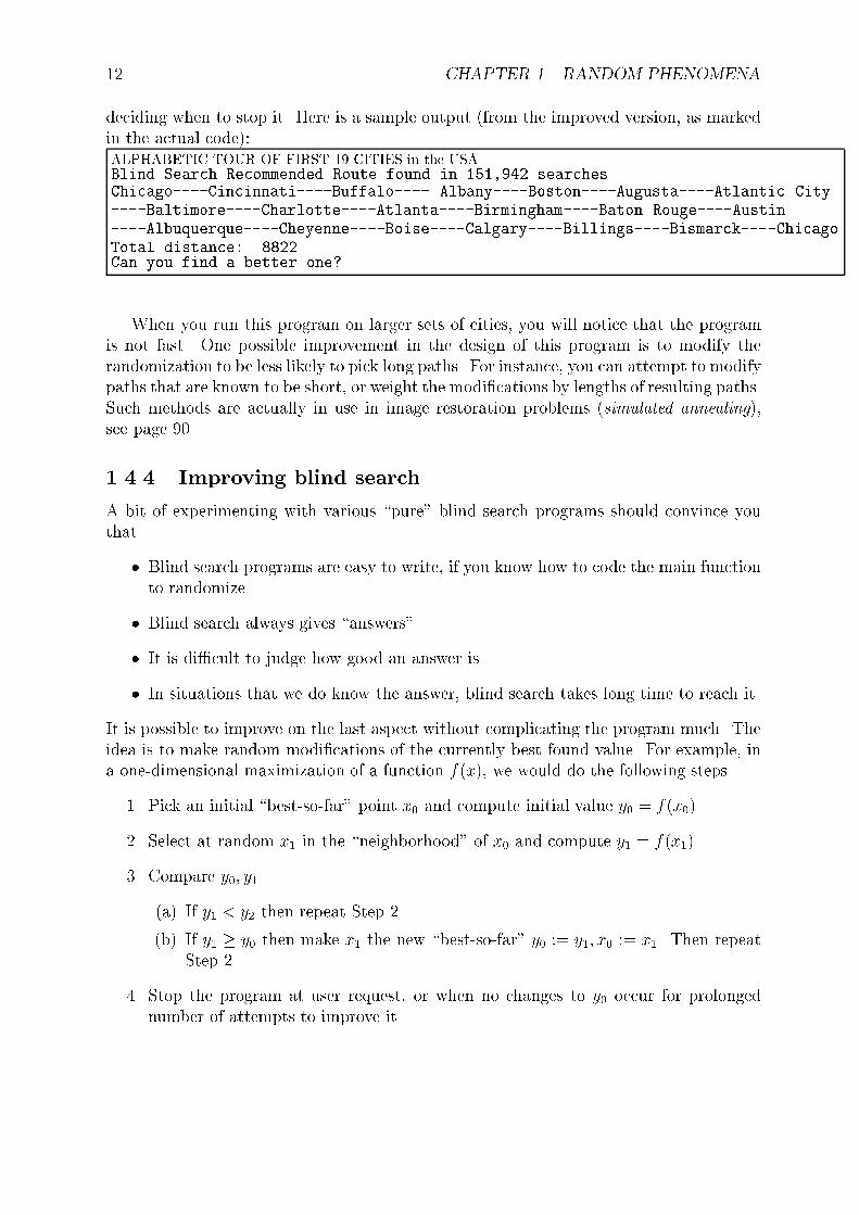
12 CHAPTER 1. RANDOM PHENOMENA
deciding when to stop it. Here is a sample output (from the improved version, as markedin the actual code):ALPHABETIC TOUR OF FIRST 19 CITIES in the USABlind Search Recommended Route found in 151,942 searches.Chicago----Cincinnati----Buffalo---- Albany----Boston----Augusta----Atlantic City----Baltimore----Charlotte----Atlanta----Birmingham----Baton Rouge----Austin----Albuquerque----Cheyenne----Boise----Calgary----Billings----Bismarck----ChicagoTotal distance: 8822Can you find a better one?
When you run this program on larger sets of cities, you will notice that the programis not fast. One possible improvement in the design of this program is to modify therandomization to be less likely to pick long paths. For instance, you can attempt to modifypaths that are known to be short, or weight the modi�cations by lengths of resulting paths.Such methods are actually in use in image restoration problems (simulated annealing),see page 90.
1.4.4 Improving blind search
A bit of experimenting with various \pure" blind search programs should convince youthat
� Blind search programs are easy to write, if you know how to code the main functionto randomize.
� Blind search always gives \answers"
� It is di�cult to judge how good an answer is.
� In situations that we do know the answer, blind search takes long time to reach it.
It is possible to improve on the last aspect without complicating the program much. Theidea is to make random modi�cations of the currently best found value. For example, ina one-dimensional maximization of a function f(x), we would do the following steps
1. Pick an initial \best-so-far" point x0 and compute initial value y0 = f(x0)
2. Select at random x1 in the \neighborhood" of x0 and compute y1 = f(x1)
3. Compare y0; y1.
(a) If y1 < y2 then repeat Step 2.
(b) If y1 � y0 then make x1 the new \best-so-far" y0 := y1; x0 := x1. Then repeatStep 2.
4. Stop the program at user request, or when no changes to y0 occur for prolongednumber of attempts to improve it.

1.4. SIMULATING DISCRETE EVENTS 13
We want to allow for the chance of checking points far away from the \best-so-far"answer. But we don't want this to happen too often, because x0 might be rather close tothe optimum. The tradeo�s are that the program will tend to follow \direct path" to themaximum, but the danger is that it will get stuck longer in local maxima.
Improved blind search with time/state dependent randomization is actually imple-mented within RANDTOUR. It is commented out in the version on the disk, so that it isn'toperational. To make it active, uncomment the call to ImproveBest as a replacement forGetPermutation.
1.4.5 Random permutations
Program RANDTOUR.BAS selects permutations at random only in its \simplest" variant.Here are a few examples of problems that require selecting random permutations.
� Card games:
{ Poker hand: Select 5 cards at random from a deck of cards.
{ Poker (2 players): Select 10 cards at random from a deck of cards.
{ Bridge: Split 52 cards into four groups
� Analyzing statistical experiments:
Suppose there are 7 items hidden under 12 cups, and a person is allowed to try to�nd them. How often all seven will be recovered by pure lack (as opposed to, say,parapsychic abilities?
The \naive" selection of random permutation wastes many random numbers. Here isan algorithm that conserves resources better. The basic idea is to select a number fromthe beginning of the list of all numbers, and move it down to the end. The randomlyre-arranged numbers are P (1); P (2); : : : ; P (n)
SUB GetPermutationFast(P())
'Put random integers into P()
n=UBOUND(P) 'how many entries
'this loop can be omitted is we are sure that P(j) list all the numbers we want
FOR j=1 TO n
P(j)=j
next j
for j=1 to UBOUND(P) 'not n as n changes in the loop
k=INT(RND(1)*n+1)
SWAP P(n), P(k)
n=n-1
next j
Exercise 1.11 There are many incompatible measures of \quality" of an algorithm. Oneof the \objective" criteria is the number of \If" veri�cations. Another \objective criterion"might be the number of calls to a function. A \subjective" criterion, which depends onthe hardware and circumstances, is timing.
Does SUB GetPermutationFast deserve adverb Fast in its name?

14 CHAPTER 1. RANDOM PHENOMENA
Project 1.12 The Subset-Sum Problem is stated as follows:Let S be a set of positive integers and let t be a positive integer. Decide of there is a
subset S 0 � S such that the sum of integers in S 0 is exactly t.The associated optimization problem is to �nd a subset S 0 � S whose elements' sum
is the largest but doesn't exceed t. This optimization problem is NP-complete, ie it isn'tknown if there is a polynomial time algorithm (polynomial in the size of S) to �nd S 0.
Investigate how the blind search will do on sets S selected at random, and on setsS constructed in more regular fashion like arithmetic progression S = fa; 2a; 3a; : : :g,geometric progression S = a; a2; a3; : : :.
1.5 Conditional probability
In modeling more complicated phenomena we may want to use di�erent probabilitiesunder di�erent circumstances. For instance, in a modi�ed blind search for the minimumof a non-negative function, the randomization strategy might be di�erent when we alreadymade some progress, and it might be di�erent when we are \stuck" in a non-optimallocation. Thus we may want to consider probabilities of the same event A (say, hitting amaximum) under di�erent conditions B.
To formalize this idea, suppose B is an event such that Pr(B) 6= 0. The last conditionmerely says that B is an event that does have some chance of occurring. Conditionalprobability of event A given event B is denoted by Pr(AjB). It is de�ned as
Pr(AjB) = Pr(A\B)Pr(B)
:
Conditional probability satis�es the axioms of probability, and Pr(AjB) = 0 if A;Bare disjoint. In particular, Pr(A0jB) = 1� Pr(AjB), Pr(BjB) = 1.
The easiest way to �nd Pr(AjB) by simulations is to repeatedly simulate the completeexperiment, discarding all the outcomes except the ones resulting in B.
Exercise 1.13 Suppose we toss repeatedly a fair coin, and the \success" is to get heads.Use computer simulations to �nd the conditional probability that the very �rst trial
was successful, if 10 consecutive (and independent) trials resulted in 8 successes.Try to answer the same question under the condition that 50 independent trials resulted
in 40 successes.
You should notice that it takes forever to simulate events that happen rarely. Section6.7 indicates one possible way out of this di�culty.
1.5.1 Properties of conditional probability
Conditional probability is used in modeling. Often Pr(AjB) can be assigned by \intuitive"considerations. It can then be used to compute other probabilities. The simplest exampleis Pr(A \ B) = Pr(B) Pr(AjB), which is a direct consequence of the de�nition.
Example 1.5 Suppose we have a deck of 52 cards numbered 1 through 52. Since it isn'tobvious how to simulate selecting 5 cards without replacement, we may want to select themwith replacement instead. Let A denote the event that all �ve cards are di�erent. Whatis the probability of A?

1.5. CONDITIONAL PROBABILITY 15
We may perform the experiment sequentially, drawing one card at a time. Let Ak
denote the event that the k consecutive draws resulted in di�erent cards. Then A = A5 �A4 � : : : � A1. Moreover, Pr(A1) = 1.
Clearly, Pr(A2jA1) =5152, so Pr(A2) = Pr(A2 \ A1) = Pr(A2jA1) Pr(A1) =
5152. Sim-
ilarly, Pr(A3) = Pr(A3 \ A2) = Pr(A3jA2) Pr(A2) = 5052
5152. Continuing this we get
Pr(A5) =51504948
524� 0:82.
The following identities are also of interest.
1. Path Probability: Pr(Tnk=1Ak) =
Qnk=1 Pr(AkjTk�1
j=1 Aj)
2. Bayes theorem: Pr(AjB) = Pr(BjA) Pr(A)Pr(B)
3. Total probability formula: If fBng are pairwise disjoint and exhaustive, ie. Pr(Ai \Bj) = ; for i 6= j and
SBn = , then
Pr(A) =Xn
P (AjBn) Pr(Bn): (1:10)
Exercise 1.14 What is the probability that in a class of 30 students no matching birthdaysoccur?
Example 1.6 A lake has 200 white �sh and a 100 black �sh, and a nearby pond contains20 black �sh and 10 white ones. No other �sh live there.
A �sh is selected at random from the lake and moved to the pond. Then a �sh isselected from the pond and moved back to the lake. What is the probability that all �sh inthe pond are black?
1.5.2 Sequential experiments
Often the main experiment consist of a sequence of sub-experiments, each depending onthe outcome of the previous one. If n such sub-experiments are chained, then the fullexperiment results in a chain of events, or a path P = A1 \ A2 \ : : : \ An. If we assumethat k-th experiment depends on the outcome of the k � 1-th experiment only, thenPr(AkjAk�1 \ : : : \ A1) = Pr(AkjAk�1).
Denoting by P the generic path A1 \ A2 \ : : : \ An, and by P(k) = Ak we have thefollowing path integral formula for the probability of an event F specifying the outcomeof the complete experiment, and consisting of many paths P.
Pr(F) = XP2F
Pr(P) = XP2F
jPjYk=0
Pr(P(k + 1)jP(k)): (1:11)
Example 1.7 Suppose that the double transfer operation from Example 1.6 was repeatedtwice. That is, a random selection was done four times. What is the probability that all�sh in the pond are black?
Exercise 1.15 Check by simulation how the proportion of black �sh in the pond changeswhen the random transfers from Example 1.6 are performed repeatedly for a long time.

16 CHAPTER 1. RANDOM PHENOMENA
1.6 Independent events
This section introduces the main modeling concept behind the entries in the Table 1.1.Two events A;B are independent, if the conditional probability is the same as uncon-
ditional, Pr(AjB) = Pr(A). This is stated in multiplicative form which exhibits symmetryand includes trivial events10
De�nition 1.6.1 Events A;B are independent if Pr(A \B) = Pr(A) Pr(B).
Independence captures the intuition of non-interaction, and lack of information. Inmodeling it is often assumed rather than veri�ed. For instance, we shall assume that theevents generated by consecutive outputs of the random generator are independent. Wealso assume that tosses of a coin (fair, or not!) are independent.
Beginners sometimes confuse disjoint versus independent events. Exclusive (ie. dis-joint) events capture the intuition of non-compatible outcomes. Not compatible outcomescannot happen at the same time. This is not the same as independent outcomes. If A;Bare disjoint and you know that A occurred, then you do know a lot about B. Namelyyou know that B cannot occur. Thus there is an interaction between A and B. Knowingwhether A occurred in uences chances of B, which is not possible under independence.
Independence (or, more properly, mutual stochastic independence) of families of eventsis de�ned by requesting a much larger number of multiplicative conditions. The reasonbehind is Theorem 1.6.1, which provides a very convenient tool.
De�nition 1.6.2 Events A1; A2; : : : ; An are independent, if Pr(Tj2J Aj) =
Qj2J Pr(Aj)
for all �nite subsets J � IN.
Example 1.8 A coin is tossed repeatedly. Find the probability that heads appears for the�rst time on the fourth toss.
Problem 1.16 SUB GetPermutation from the program RANDTOUR.BAS selects numbersbetween 1 and n at random until it �nds a number not yet on the list. Then it ads thenumber to its list, and repeats the process.
1. What is the probability that the second number added to the list required more thank attempts?
2. What is the probability that the last number added to the list required more than kattempts?
Another important concept is the conditional independence. For example, many eventsin the past and in the future are dependent. But in many mathematical models, pastand future are independent conditionally on the present situation. In such a model futuredepends on past only through present events!
De�nition 1.6.3 Let C be a non-trivial event. Events A;B are C-conditionally indepen-dent if Pr(A \BjC) = Pr(AjC) Pr(BjC).
10Trivial events are those with probabilities 0, or 1.

1.6. INDEPENDENT EVENTS 17
1.6.1 Random variables
The general concept of probability space uses \abstract" sets to represent outcomes of anexperiment. But many examples considered so far, represented the outcomes in numericalterms.
Random variables are introduced for convenient description of experiments with nu-merical outcomes. (The other option is to select � IR, or � IRd.) If we want to runcomputer simulations, we need to represent even non-numerical experiments (like tossingcoins) in numerical terms anyhow. Thus the language of random variables becomes thenatural extension of elementary probability theory, expressing many of the same conceptsin a little di�erent language.
A random variable is the numerical quantity assigned to every outcome of the ex-periment. In mathematical terms, random variable is a function X : ! IR with theproperty that sets f! 2 : X(!) � ag are events in M for all a 2 IR. Recall that thelast conditions means that we may talk about probabilities of events f! 2 : X(!) � ag.
Probabilities for a one-dimensional r. v. are determined by the cumulative distributionfunction
F (x) = Pr(X � x) (1:12)
The corresponding tail function R(x) = 1 � F (x) = Pr(X > x) is sometimes called thereliability11 function.
Cumulative distribution function can be used to express probabilities of intervalsPr(a < X � b) = F (b)�F (a). Since probability is continuous, (1.1) we can also computePr(X = a) = limb!a+ Pr(a < X � b) = F (a+) � F (a). The right hand side limit F (a+)exists, as F is a non-decreasing function.
Example 1.9 Suppose F (x) = (1� e�x) _ 0. Then Pr(jX � 2j < 1) = e�1 � e�3.
In probability theory we are concerned with probabilities. Random variables that havethe same probabilities are therefore considered equivalent. We write X �= Y to denotethe equality of distributions, ie. Pr(X 2 U) = Pr(Y 2 U) for all Borel sets U � IR (say,all intervals U).
Vector valued r. v. are measurable the functions ! IRd. In the vector case we alsorefer to X = (X1; : : :Xd) as the d-variate, or multivariate, random variable.
We will use the ordinary notation for sums and inequalities between random variables.There is however a word of caution. In probability theory, equalities and inequalitiesbetween random variables are interpreted almost surely. For instance X � Y + 1 meansPr(X � Y + 1) = 1; the latter is a shortcut that we use for the expression Pr(f! 2 :X(!) � Y (!) + 1g) = 1.
Problem 1.17 Show that F (x) = Pr(X � x) is right continuous: limx!a+ F (x) = F (a).
1.6.2 Binomial trials
The statistical analysis of repeated experiments is based on the following.
11This terminology arises under the interpretation that X represents failure time.

18 CHAPTER 1. RANDOM PHENOMENA
Theorem 1.6.1 Suppose that for j 2 IN event Bj is either Sj or S0j, where events fSjg
are independent. Then fBjg are independent.
A binomial experiment, called also binomial trials, consists of the sequence of simpleridentical experiments that have two possible outcomes each. The independent eventsSj represent successes in consecutive experiments. We assume that we have an in�nitesequence of events S1; S2; : : : Sk; : : : that are independent and have the same probabilityp = Pr(Sj). We denote by Fj = S 0j the failure in the j-th experiment, and put q = 1� p.
Two important random variables are associated with the binomial experiment are thenumber X of successes in n trials, and the number T of trials until �rst success.
Example 1.10 The probability that number X of successes in n trials is k is Pr(X =k) = (nk)p
kqn�k. (Here k = 0; : : : ; n.)
Example 1.11 The probability of more than n attempts needed for the �rst success isPr(T > n) = qn. The probability that �rst success occurs at the n-th trial is Pr(T = n) =pqn�1 (geometric).
Example 1.12 Geometric distribution has lack of memory property: Pr(T > n + kjT >n) = Pr(T > k).
Random variables are often described solely in terms of cumulative distribution functionF (x), or formulas for Pr(X = x) without reference to the underlying probability space .For instance, the number of minutes T that we spend waiting for a bird to come to thebird feeder at the back of my house is random, and I believe Pr(T = n) = pqn�1 becausePr(T > n+ kjT > n) = Pr(T > k).
It is intuitively obvious that on average we get np successes in n trials. It is perhapsless obvious12 that on average we need 1=p trials to get the �rst success.
Exercise 1.18 Write a simulation program to verify the claims about the averages forseveral values of p.
Example 1.13 The probability that in 2n tosses of a fair coin, half are heads is (2n)!4n(n!)2
�1p�n! 0 as n ! 1. The latter isn't easy to prove, but the computer printout is quite
convincing, see Table 1.2 (note that 1p�� 0:5642).
2n Pr(X = n) Frequency in 1000 trialspnPr(X = n)
100 0.07959 0.08200 0.56278300 0.04603 0.06100 0.56372500 0.03566 0.03700 0.56391700 0.03015 0.02200 0.56399
Table 1.2: Probabilities Pr(X = n) in 2n Binomial trials.
12A possible heuristic argument may argue that Tp is on average 1.

1.7. FURTHER NOTES ABOUT SIMULATIONS 19
1.7 Further notes about simulations
By now you should have written some simple simulation programs, and printed out theresults. It is perhaps a good moment to pause and consider what are the aspects ofsimulations that we are interested in.
In general, we would like to get answers to questions that we don't know how toanswer in any other way. But before we do that, we should develop some intuition on thecases that can check the answers. Therefore we begin with simulation of probabilities oraverages that are known.
A Simulation of probabilities/ averages that are known should address the followingquestions.
1. How close the simulation answers are to the theoretical answers? Print themside-by-side.
2. How large the simulation should be? Is it worth to change simulation size from1,000 to 10,000 trials? In order to answer this question, your simulation hasto provide \relative" rather than absolute answers. (Answers of the form \got32 heads" are meaningless as they depend on simulation size!)
3. How do the answers change as we change the parameters? If you did a simu-lation of the fair coin, you could change the probability p from the usual value12.
B The next natural step is to extend models that we know how to handle both theo-retically and by simulations to cover aspects that aren't easily accessible by theory.The sample questions involve
1. How would the answers change, if we allow perhaps more realistic assumptionsin the model? As an example, suppose that we would like to model the birthdayproblem with people born non-uniformly throughout the year. Which waywould you expect the answer to change?
2. What are typical errors of a simulation of size n? How can we estimate theaccuracy of the answer without having the exact answer to compare it to?Chapter 5 gives theoretical basis for such estimates.
1.8 Questions
Problem 1.19 (Exercise) A family has two children, and one of them is a boy. Whatis the probability that they have two boys? (If you think this is too hard mathematics, do
it as a computer assignment!) ANS: 1/3
Problem 1.20 (Exercise) A die is thrown until an ace turns up.Assuming the ace doesn't turn up on the �rst throw, what is the probability that more
than three throws (ie. at least four) will be necessary? ANS: 197/198
Suppose that an ace turns up on an even throw. What is the probability that it turnedup on the second throw?
(If you think this is too hard mathematics, do it as a computer assignment!)

20 CHAPTER 1. RANDOM PHENOMENA
Project 1.21 A deck of 52 cards has 4 suits and 13 values per suit.
1. Write a program simulating the hand of 5 cards.
2. Use your program to answer the following questions:
(a) How often does a pair occur?
(b) How often does a two-pair occur?
(c) How often does a three of a kind (three of same value and two di�erent) occur?
(d)
(e) How often does a four of a kind occur?
(f) How often does a full house (2+3) occur?
(g) How often does a straight (�ve cards in a row, not all same suit) occur?
(h) How often does a ush (�ve cards of one suit, not in order) occur?
(i) How often does a straight ush (�ve cards in a row all same suit) occur?
If you think this is too di�cult on a computer, compute the probabilities by hand.
Exercise 1.22 A math teacher in a certain school likes to give multiple choice tests, gradethem as either right, or wrong, and then lets the students to go over the test and correctthe ones they got wrong. This gives them two chances to get a problem right, and thechance of getting a question right increases even if the student just guesses the answers.Suppose a student simply guessed the �rst time, got the corrections, and guessed di�erentlythe second time on the wrong answers. How much his grade improves?
Project 1.23 This is the expanded version of Exercise 1.14. In a group of n people, howoften at least two have the same birthday?
1. Find the formula for the probability p(n) assuming 365 days per year, and equallylikely birthdays.
2. Compute the probabilities for n = 20; 30; 40; 50
3. Write a simulation program, and verify if the simulation agrees with the theoreticalanswers.
4. Modify the simulation program to allow for not equal birthdays. Assume January,February, March are less likely then the other days of the year. Change the param-eters, and verify how the probabilities p(n) change as you depart from the uniformprobabilities. If the change of p(n) is of the magnitude comparable to the simulationaccuracy, clearly it is irrelevant.
5. A randomly selected person has chance 1/4 to be born on a leap year. How does thisa�ect the answers?

Chapter 2
Random variables (continued)
Tree species are not distributed at random but are associated with special habi-tats.The Auborn Society Field Guide to North American Trees.
Intuitively, random variables are numerical quantities measured in an experiment. Theconcept1 is the core of probability theory; it leads outside of elementary probability andit touches advanced concepts of integration, function transforms and weak limits.
For convenience random variables are split into three groups: continuous, discrete,and the rest.
2.1 Discrete r. v.
De�nition 2.1.1 X is a discrete r. v. if X() is countable.
The de�nition says that X is a discrete r. v. if there is a �nite, or countable setV of numbers (values) of X such that pv = Pr(X = v) > 0 and
Pv2V pv = 1. The
function f(v) = pv is then called the probability mass function of X. For completeness,the domain of the probability mass function is often extended to all x 2 IR (or to x 2 IRd
in the multivariate case) by f(x) = Pr(X = x).It is easy to see that if f is a function which satis�es two natural conditions:
f(x) � 0 (2.1)Xx2IR
f(x) = 1 (2.2)
(2.3)
then there is a probability space with a random variable X such that f is its probabilitymass function. In modeling random phenomena we can therefore avoid the di�culties ofdesigning appropriate sample spaces, and pick directly relevant densities. The question, ifa density does describe the actual outcomes of experiment is to some extend the questionof statistics. Properties of various distributions, like lack-of-memory come also handywhen selecting appropriate density function.
1The precise de�nition is in Section 1.6.1.
21

22 CHAPTER 2. RANDOM VARIABLES (CONTINUED)
For discrete r. v. the cumulative distribution function (1.12) plays lesser role. It is adiscontinuous function given by the expression
F (x) =Xv�x
pv: (2:4)
This expression does show up in the \generic simulation method in Section 2.1.2.
2.1.1 Examples of discrete r. v.
Table 2.1 list the most frequently encountered discrete distributions.
Name Values Probabilities Symbol ParametersBinomial 0; : : : ; n Pr(X = k) = (nk)p
k(1� p)n�k Bin(n,p) 0 � p � 1; n 2 IN
Poisson ZZ+ Pr(X = k) = e�� �k
k!Poiss(�) � > 0
Geometric ZZ+ Pr(X = k) = p(1� p)k�1 0 � p � 1Uniform fx1; : : : ; xkg Pr(X = xj) =
1k
k 2 IN; x1; : : : ; xk 2 IRHypergeometric
Negative Binomial
Table 2.1: Discrete random variables.
Example 2.1 Let the random variable X denote the number of heads in three tosses ofa fair coin.
Example 2.2 Let the random variable X denote the score of a randomly selected studenton the �nal exam.
Problem 2.1 Let N be Poiss(�), and assume N balls are placed at random into n boxes.
Find the probability that exactly m of the boxes are empty. ANS: (nm)e��m=n(1� e
�=n)n�m .
2.1.2 Simulations of discrete r. v.
Discrete random variables with �nite number of values are simulated by assigning valuesaccording to the ranges taken by the (pseudo)random uniform random variable U from therandom number generator, U=Rand(1). To decide which value of X should be generated,take a partition f0 = a0 � a1 � : : : � an�1 � an : : : � 1g of interval (0; 1). This meansthat we simulate X = f(U) using a piecewise constant function f on the interval (0; 1).If f(x) = vk for x 2 (ak; ak+1), then Pr(X = vk) = ak+1�ak. Therefore we choose a1 = 0,a2 = p1; : : : ; ak+1 = p1 + : : :+ pk. Notice that ak = Pr(X � vk) = F (vk).
Other methods are also available for the distributions from Table 2.1. For example,program TOSSCOIN.BAS on page 7 simulates binomial distribution Bin(n=100, p=1/2).
The following exercise provides tools to run more involved simulations.
Exercise 2.2 Write functions SimOneBin(n,p) and SimOneGeom(p) that will simulate asingle occurrence of the Bin(n; p) r. v. and the geometric r. v. The sample usage: PRINTSimOneBin(15,.5) should simulate the number of heads in tossing 15 fair coins.
Also write function SimGeneric(p()) which simulates generic r. v. with values f0; 1; : : : ; ngand prescribed probabilities pk = p(k).

2.2. CONTINUOUS R. V. 23
2.2 Continuous r. v.
Continuous random variables have uncountable sets of values, and the probability of eachof them is zero, Pr(X = x) = 0 for all x 2 IR.
Since probability satis�es continuity axiom (1.1), Pr(X 2 (a; a + h)) ! 0 as h ! 0for all a. The main interest in continuous case is that the rate of convergence to 0 is alsoknown, Pr(X 2 (a; a + h)) � f(a)h + o(h). Function f(x) in this expansion is called thedensity function.
In terms of the cumulative distribution function 1.12), the probability is Pr(X 2(a; a+h)) = F (a+h)�F (a), and thus f(a) = limh!0
F (a+h)�F (a)h
= F 0(a) is the derivativeof the cumulative distribution function F . Therefore when the Fundamental Theorem ofCalculus can be invoked (say, when f is piecewise continuous)
F (x) =Z x
�1f(u) du: (2:5)
De�nition 2.2.1 Random variable X is (absolutely) continuous, if there is a function fsuch that Pr(X 2 U) =
RU f(x)dx. Function f is called the probability density function
of X.
It is known that if f is a function which satis�es two natural conditions:
f(x) � 0 (2.6)ZIRf(x) dx = 1 (2.7)
(2.8)
then there is a probability space with a random variable X such that f is its density.This is in complete analogy with the discrete case. In modeling random phenomenawe can therefore avoid the di�culties of designing appropriate sample spaces, and pickdirectly relevant densities. The question, if a density does describe the actual outcomes ofexperiment is to some extend the question of statistics. Properties of various distributionscome also handy when selecting appropriate density function.
It is convenient to use the heuristic probability density function in continuous casecorresponds to probability mass function in discrete case, and that expressions that involvein discrete case sums are replaced by integrals, compare (2.5) and (2.4).
2.2.1 Examples of continuous r. v.
The following table lists more often encountered densities. Figures 2.1 and 2.2 give thegraphs of the normal and exponential densities.
Example 2.3 A dart is thrown at a circular dart board of radius 6. Let X denote thedistance of the dart from the center. Assuming uniform assignment of probability (1.3),
the density of X is f(x) =
(x18
if 0 � x � 60 otherwise
Problem 2.3 Referring to Exercise 1.3, let X; Y denote the arrival times of the twodrivers at the intersection. Find the density of the time lapse jX � Y j between theirarrivals.
24 CHAPTER 2. RANDOM VARIABLES (CONTINUED)
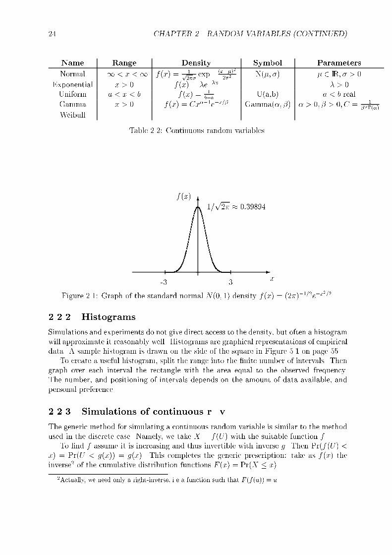
Name Range Density Symbol Parameters
Normal �1 < x <1 f(x) = 1p2��
exp� (x��)22�2
N(�; �) � 2 IR; � > 0
Exponential x > 0 f(x) = �e��x � > 0Uniform a < x < b f(x) = 1
b�a U(a,b) a < b real
Gamma x > 0 f(x) = Cx��1e�x=� Gamma(�; �) � > 0; � > 0; C = 1���(�)
Weibull
Table 2.2: Continuous random variables.
`̀̀̀`̀̀̀`̀̀̀̀`̀̀̀`̀̀̀̀`̀̀̀`̀̀̀̀`̀̀̀`̀̀̀̀`̀̀̀`̀̀̀̀`̀̀̀̀`̀̀̀`̀̀̀̀`̀̀̀`̀̀̀̀`̀̀̀`̀̀̀̀`̀̀̀`
`̀̀̀`̀̀̀``̀̀̀`̀`̀̀̀``̀̀̀``̀̀̀`̀̀`̀̀`̀̀`̀̀`̀`̀`̀̀`̀`̀`̀``̀`̀``̀``̀``̀```̀```̀``````̀`````````````````````````````````````````````̀`````̀```̀``̀`̀`̀`̀`̀`̀̀`̀̀`̀̀̀`̀̀̀``̀̀̀`̀̀̀`̀̀`̀̀`̀`̀`̀`̀`̀``̀```̀`````̀`````````````````````````````````````````````̀``````̀```̀```̀``̀``̀``̀`̀``̀`̀`̀`̀̀`̀`̀`̀̀`̀̀`̀̀`̀̀`̀̀̀`̀̀̀``̀̀̀``̀̀̀̀``̀̀̀̀`̀̀̀`̀̀̀̀`̀̀̀̀`̀̀̀
`̀̀̀̀`̀̀̀`̀̀̀̀`̀̀̀`̀̀̀̀`̀̀̀`̀̀̀̀`̀̀̀`̀̀̀̀`̀̀̀`̀̀̀̀`̀̀̀̀`̀̀̀`̀̀̀̀`̀̀̀`̀̀
x
f(x)6
-
1=p2� � 0:39894
-3 3
Figure 2.1: Graph of the standard normal N(0; 1) density f(x) = (2�)�1=2e�x2=2.
2.2.2 Histograms
Simulations and experiments do not give direct access to the density, but often a histogramwill approximate it reasonably well. Histograms are graphical representations of empiricaldata. A sample histogram is drawn on the side of the square in Figure 5.1 on page 55.
To create a useful histogram, split the range into the �nite number of intervals. Thengraph over each interval the rectangle with the area equal to the observed frequency.The number, and positioning of intervals depends on the amount of data available, andpersonal preference.
2.2.3 Simulations of continuous r. v.
The generic method for simulating a continuous random variable is similar to the methodused in the discrete case. Namely, we take X = f(U) with the suitable function f .
To �nd f assume it is increasing and thus invertible with inverse g. Then Pr(f(U) <x) = Pr(U < g(x)) = g(x). This completes the generic prescription: take as f(x) theinverse2 of the cumulative distribution functions F (x) = Pr(X � x).
2Actually, we need only a right-inverse, i.e a function such that F (f(u)) = u.

2.3. EXPECTED VALUES 25
```̀̀```̀```̀```̀``̀̀``̀``̀``̀`̀``̀``̀̀̀``̀`̀`̀`̀``̀`̀`̀`̀`̀̀̀`̀`̀`̀`̀`̀̀`̀`̀`̀`̀̀`̀`̀̀̀``̀̀`̀`̀̀`̀̀`̀̀`̀`̀̀`̀̀`̀̀̀`̀̀`̀̀̀̀``̀̀̀`̀̀`̀̀̀`̀̀̀`̀̀̀`̀̀̀`̀̀̀`̀̀̀`̀̀̀`̀̀̀``̀̀̀`̀̀̀̀`
`̀̀̀̀`̀̀̀``̀̀̀`̀`̀̀̀`̀`̀̀̀`̀`̀̀̀`̀̀`̀̀̀`̀̀`̀̀̀̀`̀`̀̀̀`̀̀̀`̀̀̀`̀̀̀`̀̀̀̀`̀̀̀`̀̀̀̀`̀̀̀`
`̀̀̀`̀̀̀`̀̀`̀̀̀̀`̀̀̀`̀
`̀̀̀̀`̀̀̀`̀̀̀`̀̀̀`̀̀̀`̀̀̀̀`̀
`̀̀̀`̀̀̀`̀̀̀̀`̀̀`̀̀̀`̀̀̀̀`̀̀̀̀`̀̀̀`
`̀̀̀`̀̀̀`̀̀̀̀`̀̀̀`̀̀̀̀`̀̀̀`̀̀̀̀`̀̀̀`̀̀̀̀`̀̀̀̀`̀̀̀
`̀̀̀̀`̀̀̀`̀̀̀̀`̀̀̀`̀̀̀̀`̀̀̀`̀̀̀̀`̀̀`̀̀̀`̀̀̀̀`̀̀̀̀`̀̀̀`̀̀̀̀`̀̀̀`̀̀̀̀`̀̀̀`̀̀̀̀`̀̀̀`̀̀̀̀
`̀̀̀`̀̀̀̀`̀
x
f(x)6
-
1.0
4.0
Figure 2.2: Graph of the exponential density f(x) = e�x as the function of x > 0.
This method of simulation is quite e�ective if the inverse of F can be found analytically.It becomes slow when the inverse (or, worse still, cumulative distribution function F itself)is computed by numerical procedures. Since this is the case of the normal distribution,special methods are used to simulate the normal distribution.
Example 2.4 To simulate X which is exponential with parameter �, use X = � 1�lnU .
2.3 Expected values
Expected values are perhaps the single most important numerical characterization of arandom phenomenon.
De�nition 2.3.1 For discrete random variable X the expected value EX is given byEX =
Pv v Pr(X = v), provided the series converges.
Expected value captures the intuition of the average of a random quantity. It is alsothis intuition that leads to estimating the expected value by averaging the outcomes ofsimulations.
Example 2.5 If X has values x1; : : : ; xn with equal probability, then EX = �x is thearithmetic mean of x1; : : : ; xn.
Simulationsare oten used to get answers that are too di�cult to �nd analytically. Thefollowing exercise can be answered by simulation if you �gure out how to shu�e cardsfrom a deck at random (Exercise 1.9).
Exercise 2.4 What is the expected number of cards which must be turned over in orderto see each of one suit.
Example 2.6 If X takes two values a < b and Pr(X = a) = p, then EX = pa+ (1� p)bis the number in the closed interval [a; b].

26 CHAPTER 2. RANDOM VARIABLES (CONTINUED)
De�nition 2.3.2 For continuous random variable X the expected value EX is given byEX =
RIR xf(x) dx, provided the integral converges.
Name Probability distribution EX
Normal f(x) = 1p2��
exp� (x��)22�2
�
Exponential f(x) = �e��x 1�> 0
Uniform f(x) = 1b�a
12(a+ b) real
GammaWeibullBinomial Pr(X = k) = (nk)p
k(1� p)n�k np
Poisson Pr(X = k) = e�� �k
k!�
Geometric Pr(X = k) = p(1� p)k�1 1p
HypergeometricNegative Binomial
Table 2.3: Expected values of some random variables.
Problem 2.5 Compute EX for the entries in Table 2.3.
Exercise 2.6 Simulate EX for the entries in Table 2.3 (except normal) for di�erentvalues of parameters involved.
Problem 2.7 (Exercise) Referring to Example 2.3, what is the average distance of adart from the center? ANS: 4 .
If you chose to do the simulations, you should perhaps notice that it is rather di�cult todecide how many simulations to take in order to achieve the desired accuracy. Typically,you need to increase the size of a simulation four times to half the error.
Another point to keep in mind is that simulations do return numbers. But fromnumbers alone it is di�clut to see how parameters of the model change it, and this is amore interesting question.
2.3.1 Tail integration formulas
The following tail integration formula is of considerable convenience in theoretical analysis.
Theorem 2.3.1 For non-negative random variables, both in the discrete, and in the con-tinuous case
EX =Z 1
0Pr(X > t) dt (2:9)
(The expected value is �nite if and only if the corresponding integral converges.)
Proof. To simplify the proof and expose the main idea more clearly, consider the dis-crete case with a �nite number of values. Similarly, to avoid technicalities we considercontinuous case with bounded range only.

2.3. EXPECTED VALUES 27
Discrete case: EX = x1p1+x2p2+ : : :+xnpn = x1(p1+p2+ : : :+pn�(p2+ : : :+pn))+x2(p2+ : : :+ pn� (p3+ : : :+ pn))+ : : :+ xn�1(pn�1+ pn� pn)+ xnpn = x1(p1+ p2+ : : :+pn)+(x2�x1)(p2+ : : :+pn�(p3+ : : :+pn))+ : : :+(xn�1�xn�2)(pn�1+pn)+(xn�xn�1)pnThe latter is
R xn0 Pr(X:t) dt.
Continuous case: Let f denote the density and F be the cumulative distribution func-tion. Integrating by parts EX =
R b0 xf(x) dx = b� R b
0 F (x) dx =R b0 (1� F (x) dx. 2
If X is discrete integer valued X 2 f0; 1; : : :g, then (2.9) can be written as
EX =1Xn=0
Pr(X > n): (2:10)
It is natural to de�ne EX for more general r. v. in the same way through formula(2.9). Write X = X+�X� to decompose X into its non-negative, and non-positive parts,and then de�ne EX =
R10 P (X > t) dt� R10 P (X < �t) dt. Clearly, if one of the integrals
diverges, EX is not de�ned.
Example 2.7 Suppose X is exponential with the density f(x) = e�x. Let Y be X trun-
cated at level 3. That is Y =
(X if X � 33 if X � 3
Clearly, Y is not continuous, as Pr(Y = 3) = Pr(X > 3) = e�3 > 0. On the otherhand, Y is not discrete as it takes uncountable number of values; in fact all the numbersbetween 0 and 3 are possible. The de�nitions of the expected value we gave do not apply,but (2.9) can be used to show that E(Y ) = 1� e�3.
Indeed, Pr(Y > t) = Pr(X > t) = e�t for 0 < t < 3, and Pr(Y > t) = 0 for t > 3.
Example 2.8 To determine the mean of the geometric distribution we can either computethe sum p
P1n=1 n(1� p)n�1, or use (2.9) and �nd the easier sum
P1n=0(1� p)n.
2.3.2 Chebyshev-Markov inequality
The following inequality is known as Markov's, or Chebyshev's inequality. Despite itssimplicity it has numerous non-trivial applications, see eg. Theorem 5.6.1.
Proposition 2.3.2 If U � 0 then
P (U > t) � EU
t(2:11)
Indeed, by (2.9) we have EU =R10 Pr(U > x) dx � R t
0 Pr(U > x) dx � tP (jXj > t).
Problem 2.8 Suppose U is uniform U(0; 1). Then Pr(U > t) � 12t. This means that
1� t < 12t.
1. Is the above inequality \sharp"? (Graph both curves).
2. Is (2.9) sharp? That is, given t > 0, is there an X > 0 such that equality occurs?

28 CHAPTER 2. RANDOM VARIABLES (CONTINUED)
2.4 Expected values and simulations
Expected value EX is approximated without much di�culty3 on a computer by averaginglarge number of independent trials.
Example 2.9 To �nd the average of the uniform U(0; 1) distribution, take 1n(U1 + : : :+
Un).
This is the basis of Monte-Carlo methods , which is a family of related probabilisticmethods for computing the integrals. To �nd
R ba f(x) dx we simulate Xj = f(a + bUj).
The average 1n
Pnj=1Xj approximates
1b�a
R ba f(u) du for large n.
The variance of the n-th approximation is of the order n�1=2, which is worse than thetrapezoidal rule for smooth functions. In return the approximation is insensitive to thesmoothness of the integrands, and also to the dimension of the integral. Monte Carlomethods can be used e�ectively for multiple integrals over irregular domains.
Exercise 2.9 Use Monte Carlo method to approximate � =R 1�1 2
p1� x2 dx. (You may
want to compare the output with numerical procedures described in Section C.1.)
Another method of similar nature is to pick points (X; Y ) at random from the rectanglecontaining the graph of f and check if Y < f(X) holds. The proportion of \successes"approximates the proportion of the area under the graph of f .
Exercise 2.10 Approximate �=4 by selecting points (X; Y ) at random from the unitsquare, and checking if X2 + Y 2 < 1.
The following sample program computes numerically double integralR R
U cos(10x +20y) dxdy over a circle x2 + y2 = 1. The only conceptual di�culty as compared to singleintegrals is how to select points at random from the unit disk. This is done by pickingpoints from a bigger square and discarding those that didn't make it. Can you do thisintegral analytically? Or by another numerical procedure?
PROGRAM dblint.bas
'
'declarations
DECLARE FUNCTION Integrand! (X!, Y!)
DECLARE FUNCTION InDomain! (X!, Y!)
CONST True = -1
' simulation loop
NumTrials = 10000
FOR j = 1 TO NumTrials
'select random points from the square [-1,1]x[-1,1]
X = 2 * RND(1) - 1
Y = 2 * RND(1) - 1
'check if this is in the domain
3Provided that limited accuracy is admissible

2.4. EXPECTED VALUES AND SIMULATIONS 29
IF InDomain(X, Y) THEN
NumTested = NumTested + 1
Sum = Sum + Integrand(X, Y)
Var = Var + Integrand(X, Y) ^ 2
END IF
NEXT j
'Print the answer
PRINT "Examined "; NumTested; " random points"
IF NumTested = 0 THEN END 'nothing found
N = NumTested
PRINT "The integral is approximately "; Sum / N
PRINT "With 95% confidence the error is less than "; 1.96 * SQR(Var / N - (Sum / N) ^ 2) / SQR
END
FUNCTION InDomain (X, Y)
'This function checks if $x,y$ is in the integration domain
'The definition of the domain can be easily modified here, including
'more complicated domains
IF X ^ 2 + Y ^ 2 < 1 THEN InDomain = True
END FUNCTION
FUNCTION Integrand (X, Y)
'This is the function to be integrated
Integrand = COS(10 * X + 20 * Y)
'
END FUNCTION
It is important to have some idea about how accurate the answer is. The programuses the Central Limit Theorem, see Section 5.4, to estimate the magnitude of the error.A less sharp (and thus safer to use!) error estimate can be obtained from (2.11)
Project 2.11 There are two natural choices to estimate by simulation events of smallprobability. We can pick a large sample size n, run the simulation experiment and hopefullyget several data points. The outcome X of such an experiment is a binomial randomvariable with unknown probability p of success, and we would estimate p � X=n. Thetrouble is that if we don't know how small the chances are, we might get none, estimatingprobability to be zero. Or we could run the experiment until we get the prescribed numberof successes. The observation would then consist of a set of geometric random variablesT1; : : : ; Tk with unknown mean ET = 1=p. We could then estimate p = 1=ET by takingthe inverse of the arithmetic mean of Tj. In this approach we are guaranteed to get someobservations, as long as p 6= 0.
The question is Which of the methods would you recommend to use? (Of course, youwould recommend a better method, but what the word \better" might mean here?)

30 CHAPTER 2. RANDOM VARIABLES (CONTINUED)
2.5 Joint distributions
Often an experiment involves measuring two or more random numbers, say X and Y .The fact that we know the distribution of X, and the distribution of Y separately doesn'tdetermine probabilities of events that involve both X and Y simultaneously.
Example 2.10 Suppose
Pr(X = 1; Y = 1) =1
4+ � (2.12)
Pr(X = �1; Y = �1) = 1
4+ �
Pr(X = �1; Y = 1) =1
4� �
Pr(X = 1; Y = �1) = 1
4� �
Then Pr(X = 1) = Pr(Y = 1) = 12regardless of the value of �. On the other hand,
Pr(X = Y ) = 12+ 2� clearly depends on the value of �.
It is clear that if X is discrete, and Y is discrete, then (X; Y ) is an IR2 valued discreter. v. That is, the values of the pair are countable. Probabilities Pr(X = x; Y = y) arecalled the joint distribution. Corresponding Pr(X = x) and Pr(Y = y) are the so calledmarginals. Example 2.10 points out that marginals do not determine joint probabilitiesuniquely. But if we know the joint probabilities then we can compute the marginals, egPr(X = x) =
Py Pr(X = x; Y = y).
In contrast to the discrete case, joint continuity can not be recognized from the con-tinuity of the components, and requires full de�nition.
De�nition 2.5.1 Let X = (X1; : : : ; Xn). Random variables X1; : : : ; Xn are jointly (ab-solutely) continuous, if there is a function f such that
Pr(X 2 U) =Z: : :ZUf(x1; : : : xn) dx1 : : : dxn
for all measurable U . Function f is then called the probability density function of X.
Example 2.11 Suppose X; Y have uniform distribution in the unit disk. Then the jointdensity is f(x; y) = 1=� for x2 + y2 � 1 and the density of X is fX(x) =
2�
p1� x2.
The relation between probabilities and the density is
f(a; b) =@2
@a@bPr(X � a; Y � b): (2:13)
Occasionally this can be used to determine the joint density.
2.6. FUNCTIONS OF R. V. 31
2.5.1 Independent random variables
Independence of random variables is de�ned in terms of joint distributions. The intuitionbehind this de�nition is that the events that random variables may generate should beindependent. Notice however that the actual de�nition is simpler than De�nition 1.6.2.Can you explain why?
De�nition 2.5.2 Random variables X1; : : : ; Xn are independent, or stochastically inde-pendent, if
Pr(X1 2 U1; : : : ; Xn 2 Un) = Pr(X1 2 U1) : : :Pr(Xn 2 Un) (2:14)
for all measurable U1; : : : ; Un � IR.
(Similarly we de�ne the stochastic independence of random vectors).We say that X1; : : : ; Xn are independent identically distributed (i. i. d) if (2.14) holds
and Pr(Xi 2 U) = Pr(Xj 2 U) for all Borel U � IR.
Proposition 2.5.1 If X; Y are discrete with the probability mass function f(x; y), thenindependence of X; Y is equivalent to f(x; y) = fX(x)fY (y).
If X; Y are continuous with the joint density f(x; y) then independence of X; Y isequivalent to f(x; y) = fX(x)fY (y).
Independence is often part of the model. Independence allows to determine jointdistributions from marginals. Thus each independent random variable can be analyzedseparately, and then more complex questions can be answered. From the mathemat-ical perspective, under independence we can determine joint distributions if we knowmarginals.
Example 2.12 Suppose X is binomial Bin(n,p) and Y is Poiss(�). If X; Y are inde-pendent, then the joint probability mass function of X; Y is given by f(x; y) = (nx)p
n(1�p)n�xe���y=y! (or 0).
Example 2.13 (Example 1.3 continued) Two drivers arrive at an intersection be-tween 8:00 and 8:01 every day. Their arrival times are independent random variables.Indeed, using formula (2.13) and elementary area computation, Pr(X < a; Y < b) = abfor 0 < a; b < 1.
2.6 Functions of r. v.
Some random variables are obtained by taking functions of another ones, possibly multi-dimensional. In the notes we often limit our attention to a single random variable Z givenby a function Z = �(X; Y ) of two arguments; this is convenient for notation and exhibitsmost of the interesting techniques.
Sums and linear combinations, medians, maxima, and minima are perhaps the mostoften encountered functions of multidimensional random variables. Methods to computethe distribution, or the expected value of such a function are of considerable practicalsigni�cance.
32 CHAPTER 2. RANDOM VARIABLES (CONTINUED)
2.7 Moments of functions
If Z = �(X; Y ) has the expected value, then EZ can be computed directly withoutcomputing the density, or probability mass function of Z. The following identity is useful.
If X; Y are discrete and EZ exists, then
E�(X; Y ) =Xx;y
�(x; y) Pr(X = x; Y = y): (2:15)
If X; Y are jointly continuous then Z might be continuous, discrete, or say of mixedtype. Regardless of the case
E�(X; Y ) =Z Z
IR2�(x; y)f(x; y) dxdy; (2:16)
and the double integral converges if EZ exists. Conversely, if the integral converges, thenEZ exists and is given by formula (2.16).
In particular the expected value is linear
E(aX + bY + c) = aEX + bEY + c: (2:17)
This can be easily veri�ed using (2.16), but the identity (2.16) is beyond the scope of thisnotes, as we do not want to dwell on the general de�nition of EZ that would encompassall cases.
The fact that expected value is linear provides a simple method of computing someotherwise di�cult sums.
Example 2.14 Suppose X is Binomial Bin(n; p). Then X = X1 + : : : +Xn, where Xj
is the number of successes in j-th trial. Clearly each Xj is 0, or 1, and EXj = p.
Exercise 2.12 (Example 1.3 continued) Two drivers arrive at an intersection be-tween 8:00 and 8:01 every day. On average how much time lapses between their arrivals?
De�nition 2.7.1 Let m = EX. The variance V ar(X) is de�ned as V ar(X) = E(X �m)2.
Notice thatV ar(aX + b) = a2V ar(X): (2:18)
In particular, V ar(X) = 0 when X = const. Sometimes a more convenient expression forthe variance is
V ar(X) = EX2 � (EX)2 = E(X � EX)2:
The standard deviation is � =qV ar(X).
Problem 2.13 Compute variances V ar(X) for the entries in Table 2.4. (Some of theseare a real challenge to your computational skills, so you may safely give up. Anothermethod will make it easier in Chapter 3).
Since V ar(X) = EX2 � (EX)2 � 0, the following inequality follows
(EX)2 � EX2 (2:19)

2.7. MOMENTS OF FUNCTIONS 33
Name Probability distribution V ar(X)
Normal f(x) = 1p2��
exp� (x��)22�2
�2
Exponential f(x) = �e��x 1�2
Uniform f(x) = 1b�a
112(b� a)2
GammaWeibullBinomial Pr(X = k) = (nk)p
k(1� p)n�k np(1� p)
Poisson Pr(X = k) = e�� �k
k!�
Geometric Pr(X = k) = p(1� p)k�1 1p2
HypergeometricNegative Binomial
Table 2.4: Variances of some random variables.
De�nition 2.7.2 The covariance of random variables X; Y with expected values mX ; mY
is de�ned as cov(X; Y ) = E(X �mX)(Y �mY ).
Clearly Cov(X;X) = V ar(X) and V ar(X + Y ) = V ar(X) + V ar(Y ) + 2cov(X; Y ).
Theorem 2.7.1 If X; Y are independent, then V ar(X + Y ) = V ar(X) + V ar(Y ).
Example 2.15 let X1; X2; : : : ; Xn be independent f0; 1g-valued random variables, andsuppose that Pr(Xj = 1) = p. Then V ar(
Pnj=1Xj) = np(1� p). What is the distribution
ofPn
j=1Xj?
Tail integration formula revisited
Example 2.16 If X > 0 then EeX = 1 +R10 etP (X > t) dt
Problem 2.14 Show that EX2 =R10 tP (jXj > t) dt.
Generalize this formula to EjXjp.
Chebyshev-Markov inequality
Special cases of Chebyshev's inequality (2.11) are:
Pr(jXj > t) <1
tEjXj (2:20)
Pr(jX � �j > t) <1
t2V ar(X) (2:21)
Pr(jXj > t) < e�atEeaX (2:22)
Chebyshev's inequality is one reason we often strive for small average quadratic error.If EjX � X0j2 < � then we can be sure that Pr(jX � X0j > 3
p�) < 3
p�. The following
may be used (with some caution) in computer programs to asses error in estimatingprobabilities by sampling.

34 CHAPTER 2. RANDOM VARIABLES (CONTINUED)
Example 2.17 If X is Bin(n; p) then Pr(jXn� pj > 1
3pn) � 1
4 3pn
Exercise 2.15 Run a simulation of the event that you know probability of, printing outthe error estimate.
Do the same for the event that you don't know the probability analytically. (Use pro-grams written for previous exercises)
2.7.1 Simulations
The unknown variance �2 of a sequence of simulated random variables Xj can be ap-proximated by 1
n
Pnj=1(Xj � �X)2, where �X is the arithmetic mean of X1; : : : ; Xn. Thus
can also use (2.21) and Theorem 2.7.1 to asses errors in estimating variances. Anothermore accurate method is presented later on in Chapter 5, but it also requires estimatingvariances.
From now on, in the output of your simulation programs you should provide someerror estimates.
2.8 Application: scheduling
A critical path analysis involves estimating time of completing a project consisting ofmany tasks of varying lengths. Some of the tasks can be done concurrently, while othermay begin only after other preliminary tasks are completed. This is modeled by thedependency graph together with the estimated times.
2.8.1 Deterministic scheduling problem
As an example of simple scheduling problem consider the following.
Example 2.18 Suppose that we want to bake a batch of chocolate-chip cookies. The tasksand their (estimated) times are:
T1 Bake at 350F (40 min)
T2 Make batter (5 min)
T3 Pre-heat oven to 350F (10 min)
T4 Find and grease pan (2 min)
T5 Find a cookie-tray to serve cookies (2 min)
T6 Take cookies out, cool and serve (5 min)
The dependency graph is quite obvious here; for instance, we cannot start baking beforebatter is ready. What is the shortest time we can eat the cookies?

2.9. DISTRIBUTIONS OF FUNCTIONS 35
2.8.2 Stochastic scheduling problem
In some projects, the actual numbers are only the averages, and the actual completiontimes of the projects may be random. The distribution of the actual completion time, oreven its average may be di�cult to compute analytically. Nevertheless, simulations let usestimate the average and analyze the probabilities of events.
Exercise 2.16 Suppose for the sake of this exercise that the numbers presented in thecookie-baking example are just the average values of the exponential random variables.
� What will be the average completion time then? Will it be larger, smaller, or aboutequal to the previous answer?
� How often will we �nish the process before the previously estimated (deterministic)time?
2.8.3 More scheduling questions
In more realistic analysis of production processes we also have to decide how to split thetasks between available personnel.
Example 2.19 This exercise refers to the tasks presented in Example 2.18. On average,how fast can a single person bake chocolate-chip cookies? What if there are two people?
2.9 Distributions of functions
Distributions of functions of random variables are often di�cult to compute explicitly.Special methods deal with more frequent cases.
Sums of discrete r. v.
Sums can be handled directly, but a more e�cient method uses generating functions ofChapter 3.
Suppose X; Y are discrete and f(x; y) = Pr(X = x; Y = y) is their joint probabilitymass function. Then Z = X + Y is discrete with values z = x+ y. Therefore
fZ(z) =Xx
f(x; z � x) (2:23)
For independent random variables X; Y this takes a slightly simpler form.
fZ(z) =Xx
fX(x)fZ(z � x) (2:24)
Formula (2.24) can be used to prove the so called summation formulas.
Theorem 2.9.1 If X; Y are independent Binomial with the same parameter p, ie. X isBin(n,p) and Y is Bin(m, p), then X + Y is Binomial Bin(n+m,p).
If X; Y are independent Poisson Poiss(�X) and Poiss(�Y ), then X + Y is PoissonPoiss(�X + �Y ).

36 CHAPTER 2. RANDOM VARIABLES (CONTINUED)
Sums of continuous r. v.
One can prove that if X; Y are independent and continuous than X + Y is continuouswith the density
f(z) =Z 1
�1fX(u)fY (z � u) du (2:25)
Formula (2.25) de�nes the convolution fX � fY . It can be used to prove the so calledsummation formulas.
Theorem 2.9.2 If X; Y are independent Normal, then X + Y is Normal.If X; Y are independent Gamma with the same parameter �, then X + Y is
Gamma(�X + �Y ; �).
Example 2.20 (Example 1.3 continued) Two drivers arrive at an intersection be-tween 8:00 and 8:01 every day. What is the density of the time that lapsed between theirarrivals?
Example 2.21 Suppose X; Y are independent U(0; 1). The density of Z = X + Y is
f(z) =
(z if 0 � z � 12� z if 1 � z � 2
.
Minima, maxima
Minima and maxima occur for instance if we are waiting for one of the independentevents, and then we follow the �rst one (minimum), or the last one (maximum). Em-bedded Markov chains construction in Section 11.2 are based on minima of independentexponential r. v.
Suppose X; Y are independent. If U = minfX; Y g then Pr(U > t) = Pr(X >t) Pr(Y > t). Therefore the reliability function of U can be computed from the twogiven ones.
Example 2.22 If X; Y are independent exponential, then U = minfX; Y g is exponential.
If U = maxfX; Y g then Pr(U < t) = Pr(X < t) Pr(Y < t). Therefore the cumulativedistribution function of U can be computed from the two given ones.
Example 2.23 Suppose X; Y are independent uniform U(0,1). Then U = maxfX; Y ghas the density f(u) = 2u for 0 < u < 1.
Problem 2.17 Let U1; : : : ; Un be independent uniform U(0; 1). Find the density of
� X = minj Uj
� Y = maxj Uj
Problem 2.18 If X; Y are independent exponential random variables with parameters�; �, show that Pr(X < Y ) = �
�+�.

2.10. L2-SPACES 37
Order statistics
Order statistics generalize minima and maxima. Their main use is in (robust) statistics,and this section can be safely skipped. Let X1; : : : ; Xn be independent continuous randomvariables with the cumulative distribution function G and density g = G0.
Let R1; : : : ; Rn be the corresponding order statistics. This means that at the endof each experiment we re-arrange the numbers X1; : : :Xn into the increasing sequenceR1; : : : ; Rn. This means that R1 = minjXj is the smallest, R2 = maximinj 6=iXj is thesecond largest, etc.
The density of Rk can be found by the following method. In order for the inequalityRk > x to hold, there must be at least k values among the Xj above level x. Since Xj areindependent and have the same probability p = Pr(Xj > x) of \success" in crossing overthe x-level, this means that Pr(Rk > x) is given by the binomial formula with n trialsand probability of success p = 1�G(x).
Pr(Rk > x) =nX
j=k
(nj )(1�G(x))j(G(x))n�j (2:26)
When the derivative is taken, the sum collapses into just one term, giving the elegantanswer rk(x) =
n!(k�1)!(n�k)!(G(x))
k(1�G(x))n�kg(x).
2.10 L2-spaces
Inequalities related to expected values are best stated in the geometric language of normsand normed spaces. We say that X 2 L2, if X is square integrable, ie. EX2 <1.
The L2 norm is
kXk2 =qEjXj2:
Notice that kX � EXk2 is just another notation for the standard deviation. Thusstandard deviation is the L2 distance of X from a constant.
We say that Xn converges to X in L2, if kXn � Xk2 ! 0 as n ! 1. We shall alsouse the phrase sequence Xn converges to X in mean-square. An example of the latter isTheorem 5.2.1.
Several useful inequalities are collected in the following4.
Theorem 2.10.1 For all square-integrable X; Y
� Cauchy-Schwarz inequality:
EXY � kXk2kY k2: (2:27)
� Jensen's inequality:EjXj � EkXk2: (2:28)
� Triangle inequality:kX + Y k2 � kXk2 + kY k2: (2:29)
4Theorem A.1.1 gives a more general statement.

38 CHAPTER 2. RANDOM VARIABLES (CONTINUED)
Proof. Proof of (2.27): Quadratic function f(t) = EjX+ tY j2 = EX2+2tEXY + t2EY 2
is non-negative for all t. Therefore its determinant � � 0. (Compute � to �nish theproof.)
Proof of (2.28): Use (2.27) with Y = 1.Proof of (2.29): By (2.27) EjX + Y j2 � kXk22 + kY k22 + 2kXk2kY k2. 2
2.11 Correlation coe�cient
Correlation is a concept deeply rooted in statistics. The correlation coe�cient corr(X; Y )is de�ned for square-integrable non-degenerate r. v. X; Y by the formula
� = corr(X; Y ) =EXY � EXEY
kX � EXk2kY � EY k2 :
The Cauchy-Schwarz inequality (2.27) implies that �1 � corr(X; Y ) � 1.Random variables with � = 0 are called uncorrelated. Correlation coe�cient close to
one of the extremes �1 means that there is a strong linear relation between X; Y ; this isstated more precisely in (2.31).
Theorem 2.7.1 states that independent random variables with �nite variances areuncorrelated.
Problem 2.19 Give an example of dependent random variables that are uncorrelated.
2.11.1 Best linear approximation
Suppose we would like to approximate random variable Y by another quantity X that isperhaps better accessible. Of all the possible ways to do it, linear function Y � mX + bis perhaps the simplest. Of all such linear functions, we now want to pick the best. In asingle experiment, the error is jY �mX � bj. We could minimize the average empiricalerror over many experiments 1
n
Pj jYj �mXj � bj. This approximates the average error
EjY �mX � bj. Let us agree to measure the error of the approximation by a quadraticerror E(Y �mX � b)2 instead. (This choice leads to simpler mathematics.)
Question: For what values of m; b the error E(Y �mX � b)2 is the smallest? Whenis it 0?
Let H(m; b) = E(Y �mX � b)2. Clearly, H is a quadratic function of m; b 2 IR. Theunique minimum is determined by the system of equations
@H
@m= 0 (2.30)
@H
@b= 0:
The answer is m = cov(X;Y )V arX
, b = EY �mEX, and the minimal error is
(1� �2)V ar(Y ): (2:31)

2.12. APPLICATION: LENGTH OF A RANDOM CHAIN 39
2.12 Application: length of a random chain
A chain in the x; y-plane consists of n links each of unit length. The angle between twoconsecutive links is ��, where � > 0 is a constant. Assume the sign is taken and random,with probability 1
2for each. Let Ln be the distance from the beginning to the end of
the chain. The angle between the k-th link and the positive x-axis is a random variableSk�1, where we may assume (why?) S0 = 0 and Sk = Sk�1 + �k�, where � = �1 withprobability 1
2. The following steps determine the average length of the random chain.
1. L2n = (
Pn�1k=0 cosSk)
2 + (Pn�1
k=0 sinSk)2.
2. E cosSn = cosn �
3. E sinSn = 0
4. E cosSm cosSn = cosn�m �E cos2 Sm for m < n
5. E sinSm sinSn = cosn�m �E sin2 Sm for m < n
6. EL2n � L2
n�1 = 1 + 2 cos� 1�cosn�1 �1�cos�
7. EL2n = n1+cos�
1�cos� � 2 cos� 1�cosn �(1�cos�)2
2.13 Conditional expectations
2.13.1 Conditional distributions
For discrete X; Y the conditional distribution of variable Y given the value of X is justthe conditional probability, Pr(Y = yjX = x). In jointly continuous case, de�ne theconditional density
f(yjX = x) =f(x; y)
fX(x):
Conditional density f(yjX = x) is de�ned only for x such that fX(x) > 0; this is areasonable approach for the most often encountered continuous, or piecewise continuousdensities. Since the densities are actually the elements of L1 space rather than functions,special care is needed in the de�nition of the conditional density. In fact the theory ofprobability is often developed without the reference to conditional distributions.
De�nition 2.13.1 The conditional expectation EfXjY = yg is de�ned asPxPr(X =
xjY = y) in discrete case, and asRIR xf(xjY = y) dx in the continuous case. One can
show that the expected values exist, when EjXj <1.
Example 2.24 A game consists of tossing a die. If the face value on the die is X thena coin is tossed X times. Let Y be the number of heads. Then E(Y jX = x) = 1
2x.
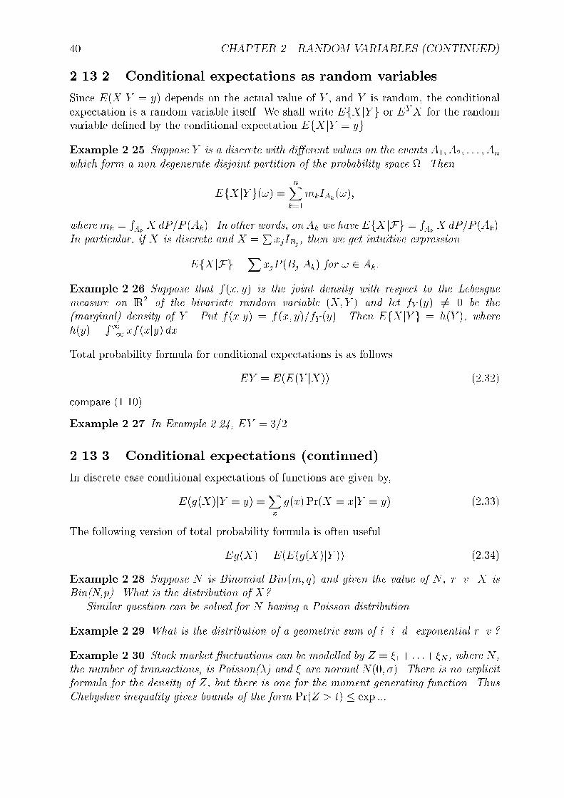
40 CHAPTER 2. RANDOM VARIABLES (CONTINUED)
2.13.2 Conditional expectations as random variables
Since E(XjY = y) depends on the actual value of Y , and Y is random, the conditionalexpectation is a random variable itself. We shall write EfXjY g or EYX for the randomvariable de�ned by the conditional expectation EfXjY = yg.Example 2.25 Suppose Y is a discrete with di�erent values on the events A1; A2; : : : ; An
which form a non-degenerate disjoint partition of the probability space . Then
EfXjY g(!) =nX
k=1
mkIAk(!);
wheremk =RAkX dP=P (Ak). In other words, on Ak we have EfXjFg = R
AkX dP=P (Ak).
In particular, if X is discrete and X =PxjIBj , then we get intuitive expression
EfXjFg =XxjP (BjjAk) for ! 2 Ak:
Example 2.26 Suppose that f(x; y) is the joint density with respect to the Lebesguemeasure on IR2 of the bivariate random variable (X; Y ) and let fY (y) 6= 0 be the(marginal) density of Y . Put f(xjy) = f(x; y)=fY (y). Then EfXjY g = h(Y ), whereh(y) =
R1�1 xf(xjy) dx.
Total probability formula for conditional expectations is as follows.
EY = E(E(Y jX)) (2:32)
compare (1.10).
Example 2.27 In Example 2.24, EY = 3=2.
2.13.3 Conditional expectations (continued)
In discrete case conditional expectations of functions are given by,
E(g(X)jY = y) =Xx
g(x) Pr(X = xjY = y) (2:33)
The following version of total probability formula is often useful.
Eg(X) = E(E(g(X)jY )) (2:34)
Example 2.28 Suppose N is Binomial Bin(m; q) and given the value of N , r. v. X isBin(N,p). What is the distribution of X?
Similar question can be solved for N having a Poisson distribution.
Example 2.29 What is the distribution of a geometric sum of i. i. d. exponential r. v.?
Example 2.30 Stock market uctuations can be modelled by Z = �1+ : : :+�N , where N ,the number of transactions, is Poisson(�) and � are normal N(0; �). There is no explicitformula for the density of Z, but there is one for the moment generating function. ThusChebyshev inequality gives bounds of the form Pr(Z > t) � exp :::.

2.14. BEST NON-LINEAR APPROXIMATIONS 41
2.14 Best non-linear approximations
This section explains the relevance of conditional expectations to the problem of bestmean-square approximation.
Theorem A.2.1 gives geometric interpretation of the conditional expectation Ef�jZg;for square integrable functions Ef:jZg is just the orthogonal projection of the Banach(normed) space L2 onto its closed subspace L2(Z), consisting of all 2-integrable randomvariables of the form f(Z).
Theorem 2.14.1 For square integrable Y the quadratic error E(Y � h(X))2 among allsquare integrable functions h(X) is the smallest if h(x) = E(Y jX = x).
Theorem 2.14.1 implies that the linear approximation from Section 2.11.1 is usuallyless accurate. In Chapter 10 we shall see that linear approximation is the best one canget in the all important normal case. Even in non-normal case linear approximationso�er quick solutions based on simple second order statistics. In contrast, the non-linearapproximations require elaborate numerical schemes to process the empirical data.
2.15 Lack of memory
Conditional probabilities help us to arrive at important classes of densities in modeling. Inthis section we want to analyze an non-aging device, which characteristics do not changewith time.
Suppose T represents a failure time of some device. If the device is working at timet, then the probability of surviving additional s seconds is Pr(T > t + sjT > t). For adevice that doesn't exhibit aging this probability should be the same as for the brandnew device.
Pr(T > t + sjT > t) = Pr(T > s) (2:35)
Problem 2.20 Show that exponential T satis�es (2.35).
Problem 2.21 Show that geometric T satis�es (2.35) for integer t; s.
Equation (2.35) implies Pr(T > t + s) = Pr(T > t) Pr(T > s), an equation that can besolved.
Theorem 2.15.1 If T > 0 satis�es (2.35) for all t; s > 0, then T is exponential.
Proof. The tail distribution function N(x) = P (T > x) satis�es equation
N(x + y) = N(x)N(y) (2:36)
for arbitrary x; y > 0. Therefore to prove the theorem, we need only to solve functionalequation (2.36) for the unknown function N(�) under the conditions that 0 � N(�) � 1,N(�) is left-continuous, non-increasing, N(0+) = 1, and N(x)! 0 as x!1.
Formula (2.36) implies that for all integer n and all x � 0
N(nx) = N(x)n: (2:37)
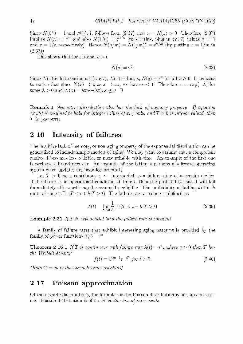
42 CHAPTER 2. RANDOM VARIABLES (CONTINUED)
Since N(0+) = 1 and N(�), it follows from (2.37) that r = N(1) > 0. Therefore (2.37)implies N(n) = rn and also N(1=n) = r1=n (to see this, plug in (2.37) values x = 1and x = 1=n respectively). Hence N(n=m) = N(1=m)n = rn=m (by putting x = 1=m in(2.37)).
This shows that for rational q > 0
N(q) = rq: (2:38)
Since N(x) is left-continuous (why?), N(x) = limq%xN(q) = rx for all x � 0. It remainsto notice that since N(x) ! 0 as x ! 1, we have r < 1. Therefore r = exp(��) forsome � > 0 and N(x) = exp(��x); x � 0. 2
Remark 1 Geometric distribution also has the lack of memory property. If equation(2.36) is assumed to hold for integer values of x; y only, and T > 0 is integer valued, thenT is geometric.
2.16 Intensity of failures
The intuitive lack-of-memory, or non-aging property of the exponential distribution can begeneralized to include simple models of aging. We may want to assume that a componentanalyzed becomes less reliable, or more reliable with time. An example of the �rst oneis perhaps a brand new car. An example of the latter is perhaps a software operatingsystem when updates are installed promptly.
Let T > 0 be a continuous r. v. interpreted as a failure time of a certain device.If the device is in operational condition at time t, then the probability that it will failimmediately afterwards may be assumed negligible. The probability of failing within hunits of time is Pr(T < t+ hjT > t). The failure rate at time t is de�ned as
�(t) = limh!0
1
hPr(T < t+ hjT > t) (2:39)
Example 2.31 If T is exponential then the failure rate is constant.
A family of failure rates that exhibit interesting aging patterns is provided by thefamily of power functions �(t) = ta.
Theorem 2.16.1 If T is continuous with failure rate �(t) = ta, where a > 0 then T hasthe Weibull density:
f(t) = Cta�1e�bta
for t > 0: (2:40)
(Here C = ab is the normalization constant).
2.17 Poisson approximation
Of the discrete distributions, the formula for the Poisson distribution is perhaps mysteri-ous. Poisson distribution is often called the law of rare events.

2.18. QUESTIONS 43
Theorem 2.17.1 Suppose Xn are Bin(n; pn) and npn ! �. Then Pr(Xn = k) !e���k=k!.
Proof. Rewrite the expression (nk)�k
nk(1��
n)n�k = �k=k!(1��=n)n=(1��=n)kQk
j=0(1�j=n).2
Example 2.32 How many raisins should a cookie have on average so that no more thanone cookie in a hundred has no raisins? So that no more than one cookie in a thousandhas no raisins?
Example 2.33 A bag of chocolate chip cookies has 50 cookies. The manufacture claimsthere are a 1,000 chips in a bag. Is it likely to �nd a cookie with 15 or less chips in sucha bag?
2.18 Questions
Problem 2.22 The performance of the algorithm for selecting a random permutation inGetPermutation SUB of RANDTOUR.BAS can be estimated by the following.
From numbers 1; : : : n, select at random k > n numbers. On average, how many ofthese numbers repeat? (and hence should be thrown out)
Problem 2.23 The performance of the algorithm for selecting a random permutationin GetPermutation SUB of RANDTOUR.BAS can be estimated by analyzing the following\worst-case" scenario.
When the algorithm attempts to select last of the random numbers 1; : : : n, then
1. What is the probability if will �nd the \right number" on �rst attempt?
2. How many attempts on average does the algorithm take to �nd the last randomnumber?
Exercise 2.24 What is the probability that in the group of 45 people one can �nd twoborn on the same day of the year? (Compare Example 1.14).
Problem 2.25 For a group of n person, �nd the expected number of days of the yearwhich are birthdays of exactly k people. (Assume 365 days in a year and that all birthdaysare equally likely.)
Problem 2.26 A large number N of people are subject to a blood test. The test can beadministered in one of the two ways:
(i) Each person can be tested separately (N tests are needed).(ii) The blood sample of k people can be pooled (mixed) and analyzed. If the test is
positive, each of the k people must be tested separately and in all k + 1 tests are thenrequired for k people.
Assume the probability p that the test is positive is the same for all people and that thetest results for di�erent people are stochastically independent.

44 CHAPTER 2. RANDOM VARIABLES (CONTINUED)
1. What is the probability that the test for a pooled sample of k people is positive?
2. What is the expected number of tests necessary under plan (ii)?
3. Find the equation for the value of k which will minimize the expected number of testsunder plan (ii).
4. Show that the optimal k is close to 1ppand hence that the minimum expected number
of tests is on average about 2Npp.
Exercise 2.27 Solve Exercise 1.3 on page 5 assuming that the arrival times are expo-nential rather than uniform. Assume independence.
Exercise 2.28 There are 3 stop-lights spaced within 1km of each other and operatingasynchronously. (They are reset at midnight.) Assuming each is red for 1 minute andthen green for one minute, what is the average time to pass through the three lights by acar that can instantaneously accelerate to 60km/h.
This exercise can be developed into a simulation project that may address some of thefollowing questions
� How does the speed change with the number of lights?
� How does the answer change if a car has �nite acceleration?
� Are the answers di�erent, if each green light lasts random amount of time, 1min onaverage?
� How to model/simulate more than one car?
� Can you simulate car tra�c on a square grid with stop-lights at intersections?
More theoretical questions
Problem 2.29 (Hoe�ding) Show that if XY;X; Y are discrete, then
EXY � EXEY =Z 1
�1
Z 1
�1(P (X � t; Y � s)� P (X � t)P (Y � s)) dt ds:
Problem 2.30 Let X � 0 be a random variable and suppose that for every 0 < q < 1there is T = T (q) such that
P (X > 2t) � qP (X > t) for all t > T:
Show that all the moments of X are �nite.
Problem 2.31 If �; U are independent, Pr(� = 0) = Pr(� + 1) = 12and U is uniform
U(0; 1). What is the distribution of U + �?

Chapter 3
Moment generating functions
3.1 Generating functions
Properties of a sequence fang are often re ected in properties of the generating functionh(z) =
Pn anz
n.
3.2 Properties
The moment generating function of a real-valued random variableX is de�ned byMX(t) =Eexp(tX). If X > 0 has the density f(x), the moment generating function is its Laplacetransform: M(t) =
R10 etxf(x) dx.
A moment generating function is non-negative, and convex (concave up). The typicalexample is the moment generating function of the f0; 1g-valued random variable.
`̀̀̀`̀̀̀̀`̀̀̀`̀̀̀̀`̀̀̀`̀̀̀̀`̀̀̀`̀̀̀̀`̀̀̀̀`̀̀̀`̀̀̀̀`̀̀̀`̀̀̀̀`̀̀̀`̀̀̀̀`̀̀̀`̀̀̀̀`̀̀̀`̀̀̀̀`̀̀̀`̀̀̀̀`̀̀̀̀`̀̀̀`̀̀̀̀`̀̀̀`̀̀̀̀`̀̀`̀̀̀̀`̀̀̀`̀̀̀̀`̀̀̀̀`̀̀̀`̀̀̀̀`̀̀̀`̀̀̀̀`̀̀̀`̀̀̀̀`̀̀̀`
`̀̀̀`̀̀̀̀`̀̀̀̀`̀̀̀`̀̀̀̀`̀̀̀`̀`̀̀̀`̀̀̀̀`̀̀̀
`̀̀̀`̀̀̀`̀̀̀`̀̀`̀̀̀`̀̀̀`̀̀̀
`̀̀̀`̀̀̀`̀`̀̀̀̀`̀̀̀
`̀̀̀`̀̀̀`̀̀̀``̀̀̀`̀̀̀̀`̀̀̀`̀̀̀`̀̀̀`̀̀`̀̀̀`̀̀`̀̀`̀̀̀̀``̀̀̀̀``̀̀̀̀`̀̀̀̀`̀̀̀``̀`̀̀̀`̀̀̀`̀̀̀`̀̀̀``̀̀̀`̀̀`̀̀`̀̀̀`̀̀``̀̀`̀̀`̀`̀̀``̀`̀̀`̀`̀`̀̀``̀`̀`̀`̀``̀``̀`̀`̀```̀`̀``
t
M(t)6
-
.75
-4 2
Figure 3.1: Graph of the moment generating function M(t) = 34+ 1
4et.
A linear transformations ofX changes the moment generating function by the following
45
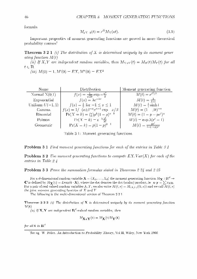
46 CHAPTER 3. MOMENT GENERATING FUNCTIONS
formula.MaX+b(t) = etbMX(at): (3:1)
Important properties of moment generating functions are proved in more theoreticalprobability courses1.
Theorem 3.2.1 (i) The distribution of X is determined uniquely by its moment gener-ating function M(t).
(ii) If X; Y are independent random variables, then MX+Y (t) = MX(t)MY (t) for allt 2 IR.
(iii) M(0) = 1;M 0(0) = EX;M 00(0) = EX2
Name Distribution Moment generating function
Normal N(0,1) f(x) = 1p2�exp�x2
2M(t) = et
2=2
Exponential f(x) = �e��x M(t) = ���t
Uniform U(�1; 1) f(x) = 12for �1 � x � 1 M(t) = 1
tsinh t
Gamma f(x) = 1=�(�)���x��1 exp�x=� M(t) = (1� �t)��
Binomial Pr(X = k) = (nk)pk(1� p)n�k M(t) = (1� p+ pet)n
Poisson Pr(X = k) = e�� �k
k!M(t) = exp �(et � 1)
Geometric Pr(X = k) = p(1� p)k�1 M(t) = pet
1�(1�p)et
Table 3.1: Moment generating functions.
Problem 3.1 Find moment generating functions for each of the entries in Table 3.1.
Problem 3.2 Use moment generating functions to compute EX; V ar(X) for each of theentries in Table 2.4.
Problem 3.3 Prove the summation formulas stated in Theorems 2.24 and 2.25
For a d-dimensional random variable X = (X1; : : : ; Xd) the moment generating functionMX : IRd !CC is de�ned byMX(t) = Eexp(t �X), where the dot denotes the dot (scalar) product, ie. x�y =
Pxkyk.
For a pair of real valued random variablesX;Y , we also writeM(t; s) =M(X;Y )((t; s)) and we callM(t; s)the joint moment generating function of X and Y .
The following is the multi-dimensional version of Theorem 3.2.1.
Theorem 3.2.2 (i) The distribution of X is determined uniquely by its moment generating functionM(t).
(ii) If X;Y are independent IRd-valued random variables, then
MX+Y(t) =MX(t)MY(t)
for all t in IRd.
1See eg. W. Feller, An Introduction to Probability Theory, Vol II, Wiley, New York 1966.
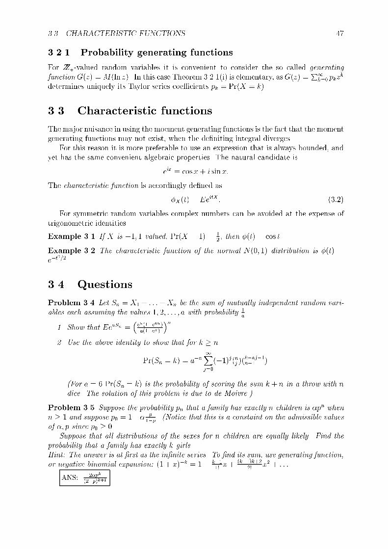
3.3. CHARACTERISTIC FUNCTIONS 47
3.2.1 Probability generating functions
For ZZ+-valued random variables it is convenient to consider the so called generatingfunctionG(z) =M(ln z). In this case Theorem 3.2.1(i) is elementary, asG(z) =
P1k=0 pkz
k
determines uniquely its Taylor series coe�cients pk = Pr(X = k).
3.3 Characteristic functions
The major nuisance in using the moement generating functions is the fact that the momentgenerating functions may not exist, when the de�niting integral diverges.
For this reason it is more preferable to use an expression that is always bounded, andyet has the same convenient algebraic properties. The natural candidate is
eix = cos x + i sinx:
The characteristic function is accordingly de�ned as
�X(t) = EeitX : (3:2)
For symmetric random variables complex numbers can be avoided at the expense oftrigonometric identities.
Example 3.1 If X is �1; 1 valued, Pr(X = 1) = 12, then �(t) = cos t.
Example 3.2 The characteristic function of the normal N(0; 1) distribution is �(t) =e�t
2=2.
3.4 Questions
Problem 3.4 Let Sn = X1 + : : :+Xn be the sum of mutually independent random vari-ables each assuming the values 1; 2; : : : ; a with probability 1
a.
1. Show that EeuSn =�eu(1�eau)a(1�eu)
�n.
2. Use the above identity to show that for k � n
Pr(Sn = k) = a�n1Xj=0
(�1)j(nj )(k�aj�1n�1 )
(For a = 6 Pr(Sn = k) is the probability of scoring the sum k + n in a throw with ndice. The solution of this problem is due to de Moivre.)
Problem 3.5 Suppose the probability pn that a family has exactly n children is �pn whenn � 1 and suppose p0 = 1�� p
1�p . (Notice that this is a constaint on the admissible valuesof �; p since p0 � 0.
Suppose that all distributions of the sexes for n children are equally likely. Find theprobability that a family has exactly k girls.Hint: The answer is at �rst as the in�nite series. To �nd its sum, use generating function,or negative binomial expansion: (1 + x)�k = 1 + k+1
1!x+ (k+1)k+2
2!x2 + : : :.
ANS: 2�pk
(2�p)k+1 .
48 CHAPTER 3. MOMENT GENERATING FUNCTIONS
Problem 3.6 Show that if X � 0 is a random variable such that
P (X > 2t) � 10 (P (X > t))2 for all t > 0;
then Eexp(�jXj) <1 for some � > 0.
Problem 3.7 Show that if Eexp(�X2) = C <1 for some a > 0, then
Eexp(tX) � C exp(t2
2�)
for all real t.
Problem 3.8 Prove that function �(t) := EmaxfX; tg determines uniquely the distribu-tion of an integrable random variable X in each of the following cases:
(a) If X is discrete.
(b) If X has continuous density.
Problem 3.9 Let p > 2. Show that exp(jtjp) is not a moment generating function.

Chapter 4
Normal distribution
Next to a stream in a forest you see a small tree with tiny, bell-shaped, white owers in dropping clusters.The Auborn Society Field Guide to North American Trees.
The predominance of normal distribution is often explained by the Central LimitTheorem, see Section5.4. This theorem asserts that under fairly general conditions thedistribution of the sum of many independent components is approximately normal. Inthis chapter we give another reason why normal distribution might occur. The usual
de�nition of the standard normal variable Z speci�es its density f(x) = 1p2�e�
x2
2 , see
Figure 2.1 on page 24. In general, the so called N(m; �) density is given by
f(x) =1p2��
e�(x�m)2
2�2 :
By completing the square one can check that the moment generating function M(t) =EetZ =
R1�1 eitxf(x) dx of the standard normal r. v. Z is given by
M(t) = et2
2 :
In multivariate case it is more convenient to use moment generating functions directly.For consistency we shall therefore adopt the following de�nition.
De�nition 4.0.1 A real valued random variable X has the normal N(m; �) distributionif its moment generating function has the form
M(t) = exp(tm +1
2�2t2);
where m; � are real numbers.
From Theorem 3.2.1 one can check by taking the derivatives that m = EX and �2 =V ar(X). Using (3.1) it is easy to see that every univariate normal X can be written as
X = �Z +m; (4:1)
49

50 CHAPTER 4. NORMAL DISTRIBUTION
where Z is the standard N(0; 1) random variable with the moment generating function
et2
2 . This is perhaps the most convenient representation1 of the general univariate normaldistribution. Traditionally, it was used to answer questions like
If X has given mean � = 123 and given variance �2 = 456, for what values ofa we have Pr(jXj > a) = :8?
with the help of tabularized values of the cumulative distribution function of standardnormal Z.
Exercise 4.1 (Basketball coach's problem) Collect data on the heights of 25 to 50randomly selected males. Make a histogram of the data, compute the empirical mean andstandard deviation.
� Does it appear that the normal distribution is a good probability distribution for theseheights?
� There are about 200,000 males in Cincinnati area. Assuming normal distributionof heights with the mean and variance as you obtained from the data, estimate thenumber of males taller than 70.
4.1 Herschel's law of errors
The following narrative comes from J. F. W. Herschel2.
\Suppose a ball is dropped from a given height, with the intention that it shallfall on a given mark. Fall as it may, its deviation from the mark is error, andthe probability of that error is the unknown function of its square, ie. of thesum of the squares of its deviations in any two rectangular directions. Now,the probability of any deviation depending solely on its magnitude, and not onits direction, it follows that the probability of each of these rectangular devia-tions must be the same function of its square. And since the observed obliquedeviation is equivalent to the two rectangular ones, supposed concurrent, andwhich are essentially independent of one another, and is, therefore, a com-pound event of which they are the simple independent constituents, thereforeits probability will be the product of their separate probabilities. Thus theform of our unknown function comes to be determined from this condition..."
Ten years after Herschel, the reasoning was repeated by J. C. Maxwell3. The fact thatvelocities are normally distributed is sometimes called Maxwell's theorem.
The beauty of the reasoning lies in the fact that the interplay of two very naturalassumptions: of independence and of rotation invariance, gives rise to the normal law oferrors | the most important distribution in statistics.
1For the multivariate analog, see Theorem 10.4.22J. F. W. Herschel, Quetelet on Probabilities, Edinburgh Rev. 92 (1850) pp. 1{573J. C. Maxwell, Illustrations of the Dynamical Theory of Gases, Phil. Mag. 19 (1860), pp. 19{32.
Reprinted in The Scienti�c Papers of James Clerk Maxwell, Vol. I, Edited by W. D. Niven, Cambridge,University Press 1890, pp. 377{409.

4.1. HERSCHEL'S LAW OF ERRORS 51
Theorem 4.1.1 Suppose random variables X; Y have joint probability distribution�(dx; dy) such that
(i) �(�) is invariant under the rotations of IR2;(ii) X; Y are independent.Then X; Y are normal.
The following technical lemma asserts that moment generating function exists.
Lemma 4.1.2 If X; Y are independent and X + Y;X � Y are independent, thenE exp aX <1 for all a.
Proof. Consider a real function N(x) := P (jXj � x). We shall show that there is x0such that
N(2x) � 8(N(x� x0))2 (4:2)
for each x � x0. By Problem 3.6 this will end the proof.Let X1; X2 be the independent copies of X. Inequality (4.2) follows from the fact that
event fjX1j � 2xg implies that either the event fjX1j � 2xg \ fjX2j � 2x0g, or the eventfjX1 +X2j � 2(x� x0)g \ fjX1 �X2j � 2(x� x0)g occurs.
Indeed, let x0 be such that P (jX2j � 2x0) � 12. If jX1j � 2x and jX2j < 2x0 then
jX1�X2j � jX1j� jX2j � 2(x�x0). Therefore using independence and the trivial boundP (jX1 +X2j � 2a) � P (jX1j � a) + P (jX2j � a), we obtain
P (jX1j � 2x) � P (jX1j � 2x)P (jX2j � 2x0)
+P (jX1 +X2j � 2(x� x0))P (jX1 �X2j � 2(x� x0))
� 1
2N(2x) + 4N2(x� x0)
for each x � x0. 2
Proof of Theorem 4.1.1. Let M(u) = EuX be the moment generating function of X.Since Eeu(X+Y )+v(X�Y ) = Ee(u+v)X+(u�v)Y
M(p2u)M(
p2v) =M(u+ v)M(u� v) (4:3)
This implies that Q(x) = lnM(x) satis�es
Q(p2u) +Q(
p2v) = Q(u+ v) +Q(u� v) (4:4)
Di�erentiating (4.4) with respect to u and then v we get
Q00(u+ v) = Q00(u� v)
Therefore (take u = v) the second derivative Q00(u) = Q00(0) = const � 0. This meansM(u) = exp(�u+ �u2). 2

52 CHAPTER 4. NORMAL DISTRIBUTION
4.2 Bivariate Normal distribution
De�nition 4.2.1 We say that X; Y have jointly normal distribution (bivariate normal),if aX + bY is normal for all a; b 2 IR.
If EX = EY = 0, the moment generating function M(t; s) = EetX+sY is given by
M(t; s) = e12(�21 t
2+2ts��1�2+s2t2)
Clearly �21 = V ar(X); �22 = V ar(Y ); � = Cov(X; Y ).When � 6= �1 the joint density of X; Y exists and is given by
f(x; y) =1q
2�(1� �2)�1�2exp�x
2 � y2 � 2��1�2xy
2�21�22(1� �2)
: (4:5)
Example 4.1 If X; Y are jointly normal with correlation coe�cient � 6= �1 then theconditional distribution of Y given X is normal.
4.3 Questions
Problem 4.2 Show that if X; Y are independent and normal, then X + Y is normal.(Hint: moment generating functions are easier than convolution formula (2.24).)
Problem 4.3 If X; Y are independent normal N(0; 1), �nd the density of X2+Y 2. (Hint:compute cumulative distribution function, integrating in polar coordinates.)
Problem 4.4 For jointly normal X; Y show that E(Y jX) = aX + b is linear.
Problem 4.5 If X; Y are jointly normal then Y � �X�Y =�X and X are independent.
Problem 4.6 If X; Y are jointly normal with variances �2X ; �2Y and the correlation co-
e�cient �, then X = �X( 1 cos � + 2 sin �, Y = �Y ( 1 sin � + 2 cos �, where j areindependent N(0; 1) and sin 2� = �.

Chapter 5
Limit theorems
This is a short chapter on asymptotic behavior of sums and averages of independentobservations. Theorem 5.2.1 justi�es simulations as the means for computing probabilitiesand expected values. Theorem 5.4.2 provides error estimates.
5.1 Stochastic Analysis
There are several di�erent concepts of convergence of random variables.
De�nition 5.1.1 Xn ! X in probability, if Pr(jXn �Xj > �)! 0 for all � > 0
Example 5.1 Let Xn be N(0; � = 1n). Then Xn ! o in probability.
De�nition 5.1.2 Xn ! X almost surely, if Pr(Xn ! X) = 1.
Example 5.2 Let U be the uniform U(0,1) r. v. Then 1nU ! 0 almost surely.
Example 5.3 Let U be the uniform U(0,1) r. v. et Xn =
(0 if U > 1
n
1 otherwise. Then
Xn ! 0 almost surely.
De�nition 5.1.3 Xn ! X in L2 (mean square), if EjXn �Xj2 ! 0 as n!1.
Remark 2 If Xn ! X in L2, then by Chebyshev's inequality Xn ! X in probability.If Xn ! X almost surely, then Xn ! X in probability.
5.2 Law of large numbers
Each law of large numbers (there are many of them) states that empirical averages con-verge to the expected value. In statistical physics the law of large numbers impies thattrajectory averages and population averages are asymptoticaly the same. In simulations,it provides a theoretical foundation, and connects the frequency with the probability ofan event.
53
54 CHAPTER 5. LIMIT THEOREMS
Theorem 5.2.1 Suppose Xk are such that EXk = �; V ar(Xk) = �2, and cov(Xi; Xj) = 0for all i 6= j. Then 1
n
Pnj=1Xj ! � in L2
Proof. To show that 1n
Pnj=1Xj ! � in mean square, compute the variance. 2
Corollary 5.2.2 If Xn is Binomial Bin(n; p) then 1nXn ! p in probability.
5.2.1 Strong law of large numbers
The following method can be used to prove strong law of large numbers for Binomial r. v.
1. If X is Bin(n; p), use moment generating function to show that E(X � np)4 � Cn2
2. Use Chebyshev's inequality and fourth moments to show thatP
n Pr(jXn=n� pj >�) <1.
3. Use the convergence of the series to show that limN!1 Pr(Sn�NfjXn=n�pj > �g) =
0.
4. Use the continuity of the probability measure to show that Pr(TN
Sn�NfjXn=n �
pj > �g) = 0.
5. Show that with probability one for every rational � > 0 there is N = N(�) such thatfor all n > N the inequality jXn=n� pj < � holds. Hint: if Pr(A�) = 1 for rational�, then Pr(
T�A�) = 1.
5.3 Convergence of distributions
In addition to the types of convergence introduced in Section 5.1, we also have the con-vergence in distribution.
De�nition 5.3.1 Xn converges to X in distribution, if Ef(Xn)! Ef(X) for all boundedcontinuous functions f .
Theorem 5.3.1 If Xn ! X in distribution, then Pr(Xn 2 (a; b)) ! Pr(X 2 (a; b)) forall a < b such that Pr(X = a) = Pr(X = b) = 0.
Theorem 5.3.2 If MXn(u)!MX(u) for all u, then Xn ! X in distribution.
Theorem 2.17.1 states convergence in distribution to Poisson limit. Here is a proofthat uses moment generating functions.Proof of Theorem 2.17.1. MXn(u) = (1 + pn(e
u � 1))n ! e�(eu�1). 2
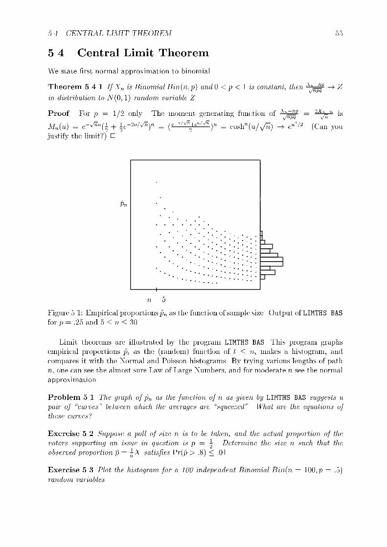
5.4. CENTRAL LIMIT THEOREM 55
5.4 Central Limit Theorem
We state �rst normal approximation to binomial.
Theorem 5.4.1 If Xn is Binomial Bin(n; p) and 0 < p < 1 is constant, then Xn�nppnpq
! Z
in distribution to N(0; 1) random variable Z.
Proof. For p = 1=2 only. The moment generating function of Xn�nppnpq
= 2Xn�npn
is
Mn(u) = e�pnu(1
2+ 1
2e�2u=
pn)n = ( e
�u=pn+eu=pn
2)n = coshn(u=
pn) ! eu
2=2. (Can youjustify the limit?) 2
` ` ` ` ` ` `
``
``
` `
``
`
`
``
`
``
``
`
` ` ` ` ` ` ` `
``
`
``
`
`
`
`
`
``
``
``
`
`
`
`
`
`
`
`
`
`
`
`
`
`
`
`
`
`
`
`
`
`
`
`
`
`
`
`
`
`
`
`
`
`
`
`
`
`
`
`
`
`
`
`
`
`
`
`
`
`
`
`
`
`
`
`
`
`
`
`
`
`
`
`
`
`
`
`
`
`
`
`
`
`
`
`
`
`
`
`
`
`
`
`
`
`
`
`
`
`
`
`
`
`
`
`
`
`
`
`
`
`
`
`
`
`
`
`
`
`
`
`
`
`
`
`
`
`
`
`
`
`
`
``
`
`
`
`
`
`
`
`
`
`
`
`
`
`
`
`
`
`
`
`
`
`
`
`
`
`
`
`
`
`
`
`
``
`
`
`
`
`
``
`
`
``
`
``
``
`
`
`
`
`
`
`
`
`
`
`
`
`
`
`
`
`
`
`
`
`
`
`
`
`
`
`
`
`
`
`
`
`
`
`
`
`
`
`
`
`
`
`
`
`
`
`
``
`
`
` ` `
`
`
`
``
`
`
`
`
`
``
``
``
`
``
``
`
`
`
`
`
`
`
`
`
`
`
`
`
`
`
`
`
`
`
`
`
`
`
``
`
`
`
`
`
`
`
`
`
`
`
`
`
`
`
`
`
`
`
`
`
`
`
``
`
` `
`
`
`
`
`
`
`
`
`
`
`
`
`
`
`
``
`
``
``
``
`
`
`
`
`
`
`
`
``
``
``
`
`
``
`
`
`
``
`
`
`
`
`
`
`
`
`
`
`
`
`
`
`
`
`
`
`
`
`
`
`
`
`
`
`
`
`
`
`
`
`
`
`
`
`
`
`
`
`
`
`
`
`
`
`
``
`
`
`
`
`
`
`
`
`
`
`
`
`
`
`
`
`
`
`
`
`
`
`
`
`
`
`
`
`
`
`
`
`
`
`
`
`
`
`
`
``
`
`
`
`
`
`
`
`
`
`
` ` ` ` ` ` `
``
``
`
`
``
`
`
``
`
``
`
`
`
`
`
`
`
`
`
`
`
`
`
`
`
`
`
`
`
`
`
``
`
`
`
`
`
`
`
`
`
`
`
`
`
`
`
`
`
`
`
`
`
`
`
`
`
`
`
`
`
`
`
`
`
`
`
`
`
`
`
`
`
`
`
`
`
`
`
`
`
`
`
`
`
`
`
`
`
`
`
`
`
`
`
`
`
`
`
`
`
`
`
`
`
`
`
`
`
`
`
`
`
`
`
`
`
`
`
`
`
`
`
`
`
`
`
`
`
`
`
`
`
``
`
`
`
`
`
`
`
`
`
`
`
`
`
`
`
`
`
`
`
`
`
`
`
``
`
`
`
`
`
`
`
`
`
`
`
`
`
`
`
`
`
`
`
`
``
``
``
`
`
`
`
`
`
`
`
`
`
`
`
`
`
`
`
`
`
`
``
`
`
``
`
` `
`
`
`
`
`
`
`
`
`
`
`
`
`
`
`
``
`
``
``
`
`
`
`
`
`
`
`
`
`
`
`
`
`
`
`
`
`
`
`
`
`
`
`
`
``
`
`
`
`
`
`
`
`
`
`
`
`
`
`
`
`
`
`
`
`
`
`
`
`
`
`
`
`
`
`
`
`
`
`
`
`
`
`
`
`
`
`
`
`
`
`
`
`
`
`
`
`
`
`
`
`
`
`
`
`
`
`
`
`
`
`
`
`
`
`
`
`
`
`
` ` `
`
`
`
``
``
`` `
``
``
``
``
``
``
`
`
`
`
`
`
`
`
`
`
`
`
`
`
`
`
`
`
``
`
``
`
`
`
`
`
`
`
`
`
`
`
``
``
``
``
`` `
`` `
`
`
` ` ` ` ` ` `
``
``
``
`
`
`
`
``
`
``
`
``
`
`
`
`
`
`
`
`
`
`
`
`
`
`
`
`
`
`
`
`
`
``
`
`
` ` `
`
`
`
`
`
`
``
``
`
`
`
`
``
`
`
`
``
`
` ` ` ` ` ` ` ` ` ` `
` `` `
`
``
`
`
``
`
``
`
`
`
`
`
`
`
`
`
`
`
`
`
`
`
`
`
`
``
`
`
``
`
`
`
`
`
`
`
`
`
`
`
`
`
`
`
`
`
`
`
`
`
`
`
`
`
`
`
`
`
`
`
`
`
`
`
``
``
`
`
``
``
``
``
` `
`
`
`
`
`
`
`
`
`
`
`
`
`
`
`
`
`
`
`
`
`
`
`
`
`
`
`
`
`
`
`
`
`
`
`
`
`
`
``
``
``
``
``
` `
` ` ` ` ` ` `
``
``
`
`
``
``
``
`
`
`
``
`
`
`
`
`
`
`
`
`
`
`
`
`
`
`
`
`
`
``
`
``
``
`
`
`
`
`
`
`
`
`
`
`
`
`
`
`
`
`
`
`
`
`
`
``
`
`
`
`
`
`
`
`
`
`
`
`
`
`
`
`
`
`
`
`
`
`
`
`
`
`
`
p̂n
n = 5
Figure 5.1: Empirical proportions p̂n as the function of sample size. Output of LIMTHS.BASfor p = :25 and 5 � n � 30
Limit theorems are illustrated by the program LIMTHS.BAS. This program graphsempirical proportions p̂t as the (random) function of t � n, makes a histogram, andcompares it with the Normal and Poisson histograms. By trying various lengths of pathn, one can see the almost sure Law of Large Numbers, and for moderate n see the normalapproximation.
Problem 5.1 The graph of p̂n as the function of n as given by LIMTHS.BAS suggests apair of \curves" between which the averages are \squeezed". What are the equations ofthese curves?
Exercise 5.2 Suppose a poll of size n is to be taken, and the actual proportion of thevoters supporting an issue in question is p = 1
2. Determine the size n such that the
observed proportion p̂ = 1nX satis�es Pr(p̂ > :8) � :01.
Exercise 5.3 Plot the histogram for a 100 independent Binomial Bin(n = 100; p = :5)random variables.

56 CHAPTER 5. LIMIT THEOREMS
Theorem 5.4.2 If Xj are i.i.d. with EX = �; V ar(X) = �2 then
Pn
j=1Xj�n�
�pn
! Z
Proof. For � = 0; � = 1 only.The moment generating function is Mn(u) = (M1(u=
pn))
n= (1 + up
nM 0(0) +
u2
2nM 00(0) +O( 1
n2))n ! eu
2=22
A lesser known aspect of the central limit theorem is that one can actually simulatepaths of certain continuous time processes by taking Xn(t) =
1pn
Pk�nt �k, where �k are
independent mean-zero r. v.The following program uses this to simulate random curves. The program requires a
graphics card on the PC.
PROGRAM firewalk.bas
'
'This program simulates random walk paths (with uniform incerments)
'reflected at the boundaries of a region
'
'declarations of subs
DECLARE SUB CenterPrint (Text$)
' minimal error handling - graphics card is required
ON ERROR GOTO ErrTrap
CLS
'request good graphics (some cards support SCREEN 7, etc)
SCREEN 9
LOCATE 1, 1 'title
CenterPrint "Path of reflected random walk"
LOCATE 9, 1 'timer location
PRINT "Timer"
scale = 10 '
WINDOW (0, 0)-(scale, scale): VIEW (150, 100)-(600, 300)
LINE (0, 0)-(scale, scale), 10, B': LINE (scale, scale)-(2 * scale, 0), 11, B
FOR j = -4 TO 4
LINE (0, scale / 2 + j)-(scale / 50, scale / 2 + j), 2
NEXT j
X = scale / 2
Y = scale / 2
dead = 0
T = 0
col = 14 * RND(1)
speed = scale / 100
WHILE INKEY$ = "" 'infinite loop until a key is pressed
T = T + 1
X0 = X
Y0 = Y
X = X + (RND(1) - 1 / 2) * speed
Y = Y + (RND(1) - 1 / 2) * speed
IF X < 0 THEN X = -X: col = 14 * RND(1)
IF Y < 0 THEN Y = -Y: col = 14 * RND(1)
IF X > scale THEN X = 2 * scale - X: col = 14 * RND(1)

5.5. LIMIT THEOREMS AND SIMULATIONS 57
IF Y > scale THEN Y = 2 * scale - Y: col = 14 * RND(1)
IF X > 2 * scale THEN X = 4 * scale - X: col = 14 * RND(1)
LINE (X0, Y0)-(X, Y), col
LOCATE 10, 1
PRINT T
WEND
END
ErrTrap: 'if there are errors then quit
CLS
PRINT "This error requires graphics card VGA"
PRINT "Error running program"
PRINT "Press any key ...'"
WHILE INKEY$ = ""
WEND
END
SUB CenterPrint (Text$)
' Print text centered in 80 column screen
offset = 41 - LEN(Text$) \ 2
IF offset < 1 THEN offset = 1
LOCATE , offset
PRINT Text$
'
END SUB
5.5 Limit theorems and simulations
One role of limit theorems is to justify the simulations and provide error estimates. Thesimulation presented on page 28 uses the Central Limit Theorem to print out the so called95% con�dence interval.
Central limit theorem is also a basis for a fast simulation of the normal distribution,see Section 6.3.3.
5.6 Large deviation bounds
We begin with the bound for binomial distribution.Recall that the relative entropy is H(qjp) = �q ln q=p� (1� q) ln 1�q
1�p .
Theorem 5.6.1 Suppose Xn is Binomial Bin(n; p). Then for p0 � p
Pr(1
nXn � p0) � exp nH(p0jp) (5:1)
Proof. Use Chebyshev's inequality (2.22) and the moment generating function.
Pr(Xn � np0) = Pr(uXn � unp0) � e�np0uEuXn =
�e�p
0u(1� p+ peu)�n
=�(1� p)e�p
0u + pe(1�p0)u�n.

58 CHAPTER 5. LIMIT THEOREMS
Now the calculus question: for what u � 0 the function f(u) = (1� p)e�p0u+ pe(1�p
0)u
attains a minimum? The answer is u = 0 if p0 � p, or u = ln(1�pp
p0
1�p0 ). Therefore the
minimal value is f(umin) =pp0 e
(1�p0)u = exp(�p0 ln p0=p� (1� p0) ln(1� p0)=(1� p)) 2
Corollary 5.6.2 If p = 1=2 then
Pr(j 1nXn � 1
2j > t) � e�nt
2=2 (5:2)
Proof. This follows from the inequality (1 + x) ln(1 + x) + (1� x) ln(1� x) � x2. 2
5.7 Conditional limit theorems
Suppose Xj are i.i.d. Conditional limit theorems say what is the conditional distributionof X1, given the value of the empirical average 1
n
Pnj=1 h(Xj). Such probabilities are
di�cult to simulate when 1n
Pnj=1 h(Xj) di�ers signi�cantly from Eh(X).
5.8 Questions
Exercise 5.4 A 400-point multiple choice test has four possible responses, one of whichis correct.
� What proportion of students that just guess the answer gets the score of more than100? Of more than 110? Of more than 130?
� What proportion of students that know how to answer corectly 20% of question getsthe score of more than 100? of more than 130? Of more than 180?
� What proportion of problems you know how to answer corectly in order to have a fairshot at A, which requires a score of at least 361? (For the purpose of this exercisea fair shot is 75% chance.)

Part II
Stochastic processes
59


Chapter 6
Simulations
This chapter collects information about how to simulate special distributions.Considerations of machine e�ciency, in particular convenience of doing �xed precision
arithmetics, make the uniform U(0; 1) the fundamental building block of simulations. Wedo not consider in much detail how such sequences are produced { e�cient methods arehardware-dependent. We also assume these are i. i. d., even though the typical randomnumber generator returns the same pseudo-random sequence for each value of the seed,and often the sequence is periodic and correlated. This is again a question of speed andhardware only.
6.1 Generating random numbers
Suppose x0 is an arbitrary number between 0 and 1 with 5 decimal places or more. Letx1 = f147x0g, and xn+1 = f147xng, where fag = a � [a] denotes the fractional part.Here are the questions: Is xn a random sequence? Does it have \enough" propertries ofa random sequence to be used for simulations?
6.1.1 Random digits
The classical Peano curve actually maps the unit interval onto the unit square preservingthe Lebesgue measure. Thus two independent U(0; 1) are as \random" as one!
Experiments with discrete outcomes aren't necessarily less random than continuousmodels. Expansion into binary fractions connects in�nite tosses of a coin with a singleuniform r. v.
Example 6.1 Let U be uniform U(0; 2�). Random variables Xk = sign(sin(2kU)) arei. i. d. symmetric independent.
Theorem 6.1.1 If �j are independent identically distributed discrete random variableswith values f0; 1g and Pr(� = 1) = 1=2 then
P1k=1
12k�k in uniform U(0; 1).
Proof. We show by induction that if U is independent of f�jg uniform U(0; 1) r. v., then12nU +
Pnk=1
12k�k is uniform for all n � 0. For induction step, notice that in distribution
12nU +
Pnk=1
12k�k �= 1
2�1 +
12U . This reduces the proof to n = 1 case.
61
62 CHAPTER 6. SIMULATIONS
The rest of the proof is essentially the solution of Problem 2.31. Clearly Pr(12�1+
12U <
x) = Pr(�1 = 0)Pr(U=2 < x) + Pr(�1 = 1)Pr(12+ U=2 < x) Expression Pr(U=2 < x) is
0; 2x; or 1. Expression Pr(12+ U=2 < x) is 0; 2x� 1; or 1. Their average (check carefully
ranges of x!) is
8><>:
0 if x < 0x if 0 � x � 11 if x > 1
2
Coe�cient 2 does not play any special role. The same fact holds true in any numbersystem - if N > 1 is �xed, and U =
PXjN
�j is expanded in pase N , then Xj areindependent uniform f0; 1; : : : ; N � 1g-valued discrete random variables.
From the mathematical point of view all of the simulations can be based on a sin-gle U(0; 1) random variable. In particular, to generate independently uniform integernumbers1 in the prescribed range 0 : : : N we need to pick any u 2 (0; 1), and de�neXj = N ju mod N .
Clearly Xj is the integer part of NUj, where Uj solve the recurrence
Uj+1 = fUjNg (6:1)
and fg denotes the fractional part. A computer realization of this construction would useUj = nj=M with some M > N , Thus nj+1 = Nnj modM .
Many programs provide access to uniform numbers. These however might be platform-dependent, and are often of \low quality". Often a person performing simulation maywant to use the code they have explicit access to. What is \random enough" for oneapplication may not be random enough for another.
6.1.2 Overview of random number generators
There is good evidence, both theoretical (see (6.1)) and empirical, that the simple multi-plicative congruential algorithm
nj+1 = anj (mod N) (6:2)
can be as good as the more general linear congruential generator. Park & Miller proposea minimal standard generator based on the choices a = 75; N = 231 � 1. The computerimplementation of this method is not obvious due to over ows when multippying largeintegers in �nite computer arithmetics, see Schrage's algorithm in [23].
The linear congruential method has the advantage of being very fast. It has thedisadvantage that it is not free of sequential correlations between successive outputs. Thisshows up clearly in the fact that the consecutive k-points lie in at most N1=k subspacesof dimension k � 1.
Many system-supplied random number generators are linear congruential generators,which generate a sequence of integers n1; n2; : : : each between 0 andN�1 by the recurrencerelation
nj+1 = anj + b mod N (6:3)
1This is all we can hope for in the �nite computer arithmetics. Whenever Uj 2 (0; 1) is selectedand �nite approximation is chosen, Nj = NUj is an integer, where N = 2b is the characteristic of theoperating system.

6.2. SIMULATING DISCRETE R. V. 63
The value of N is the largest integer representable in the machine. This is 216 on 16-bitmachines, unless long integers are used (then it is 232). Value used in C-supplied generatorare a = 1103515245; b = 12345; N = 232.
6.2 Simulating discrete r. v.
6.2.1 Generic Method { discrete case
Section 2.1.2 described the generic method for simulating a discrete random variableswith �nite number of values. Namely, take X = f(U), where f is a suitable piecewiseconstant functions on the interval (0; 1). Let Pr(X = vk) = pk. Then f(x) = vk forx 2 (
Pkj=1 pj;
Pk+1j=1 pj).
This is rather easy to convert into the computer algorithm.
6.2.2 Geometric
A simple method for simulating geometric distribution is to simulate independent binomialtrials until the �rst success.
6.2.3 Binomial
A simple method for simulating Binomial Bin(n; p) random variable is to simulate bino-mial trials with the prescribed probability of success. For a sample program illustratingthis method, see TOSSCOIN.BAS page 7.
6.2.4 Poisson
An exact method to simulate Poisson distribution is based on the fact that it occurs thePoisson process, and that sojourn times in the Poisson process are exponential (see The-orem 11.1.1 on page 103). Therefore, to simulateX with Poiss(�) distribution, simulateindependent exponential r. v. T1; T2; : : : ; with parameter � = 1 and put as the value ofX the �rst value of n such that T1 + : : :+ Tn > �.
A reasonable approximation to Poisson Poiss(�) random variable X is obtained bysimulating binomial Bin(n; p) random variable X 0 with � = np. Since X 0 � n, use nlarge enough to exceed any realistic values of X. Run program LIMTHMS.BAS to comparethe histograms { why is Poisson distribution more spread out than the binomial?
6.3 Simulating continuous r. v.
6.3.1 Generic Method { continuous case
Section 2.2.3 described the generic method for simulating a continuous random variable,similar to the method used in the discrete case. Namely, take X = f(U) where f is theinverse2 of the cumulative distribution functions F (x) = Pr(X � x).
2Actually, we need only a right-inverse, i.e a function such that F (f(u)) = u.

64 CHAPTER 6. SIMULATIONS
Problem 6.1 Given a cumulative distribution function G(x) with inverse H(), and den-sity g(x) = G0(x), let U1; U2 be two independent uniform U(0; 1) random variables. Showthat X = H(U1); Y = U2g(X) are uniformly distributed in the region f(x; y) : 0 < y <g(x)g.
6.3.2 Randomization
If the conditional density of Y given X = x is f(yjx), and the density of X is g(x), thenthe density of Y is
R(f(yjx)g(x) dx.
As an example, suppose Y has density cye�y = CP1
n=0 y(1 � y)n=n!. Let Pr(X =n) = c=n!. Then the conditional distribution is f(yjX = n) = Cy(1� y)n, which is thedistribution of a median from the sample of size 2n.
6.3.3 Simulating normal distribution
By the central limit theorem (Theorem 5.4.2), if U1; : : : ; Un are i. i. d. uniform U(0; 1)
thenq
12n
Pnk=1(Uk� 1
2) is asymptotically normalN(0; 1). In particular a computer-e�cient
approximation to normal distribution is given by
12Xk=1
Uk � 6:
The exact simulation of normal distribution uses the fact that an independent pairX1; X2 of normal N(0; 1) random variables can be written as
X1 = R cos� (6.4)
X2 = R sin� (6.5)
where � is uniform U(0; 2�), R =pX2 + Y 2 is exponential (see Problem 4.3) with
parameter � = 12, and random variables �; R are independent. Clearly R =
p�2 lnU ,see Example 2.4.
We simulate two independent normal N(0; 1) r. v. from two independent uniform r. v.U1; U2 by taking � = 2�U1; R =
p�2 lnU2 and using formulas (6.4)-(6.5).
6.4 Rejection sampling
The idea of rejection method is very simple. In order to simulate a random variable withthe density f(x), select a point X; Y at random uniformly from the region f(x; y) : y <g(x)g. Then Pr(X < x) =
R x�1 f(t) dt is the cumulative distribution function, which we
do not have to know analytically.The name comes from the technique suggested by Problem 6.1. Instead of selecting
points under the graph of f(x), we pick another function g(x) > f(x), which has knownantiderivative with explicitly available inverse. We pick points under the graph of g(x),and "reject" those that didn't make it below the graph of f(x).
Often used density g(x) = c=(1 + x2) leads to X = H(U1), where H(u) = tan(�u=c).

6.5. SIMULATING DISCRETE EXPERIMENTS 65
Rejection sampling can be used to simulate continuous or discrete distributions. Theidea behind using it in discrete case is to convert discrete distribution to a function of con-tinous random variable. For example, to use rejection sampling for Poisson distribution,simulate the density f(x) = e���[x]=[x]! and take the integer part [X] of the resultingrandom variable.
6.5 Simulating discrete experiments
6.5.1 Random subsets
To simulate uniformly selected random subsets of f1; : : : ; ng, de�ne sets by a sequencesS(j) 2 f0; 1g with the interpretation j 2 S if S(j) = 1. Now select independently 0 or 1with probablity 1
2for each of the values of S(j); j = 1; : : : ; n.
SUB RandomSubset( S())
n = UBOUND(S) ' read out the size of array
FOR j = 1 TO n
'select entries at random
S(j) = INT(RND(1) + 1)
NEXT j
For subsets of low dimension, a sequence of 0; 1 can be identi�ed with binary numbers.Set operations are then easily converted to binary operations on integers/long integers.
6.5.2 Random Permutations
Suppose we want to re-arrange elements a(1); : : : ; a(n) into a random order. A quickmethod to accomplish this goal is to pick one element at a time, and set it aside. Thiscan be easily implemented within the same sequence.
SUB Rearrange( A())
n = UBOUND(A) ' read out the size of array
ns = n 'initial size of randomization
FOR j = 1 TO n
'take a card at random and put it away
k = INT(RND(1) * ns + 1)
SWAP A(k), A(ns)
ns = ns - 1 'select from remaining a(j)
NEXT j
Problem 6.2 Let a1; : : : an be numbers such thatP
j aj = 0;P
j a2j = 1 Let X denote the
sum of the �rst half of those numbers, after a random rearrangement.
� Find E(X), V ar(X).
� Under suitable conditions, as n ! 1, the distribution of X is asymptotically nor-mal. Verify by simulations.
� Let Y be the sum of the �rst 14of aj after random rearrangement. Find E(XjY )
and E(Y jX).

66 CHAPTER 6. SIMULATIONS
6.6 Integration by simulations
Program listing on page 28 explains how to perform double integration by simulation. Herewe concentrate on re�ning the procedure for single integrals by reducing the variance.
To evaluate J =R ba f(x) dx we may use the approximation
1N
PNj=1 f(Xj)=g(Xj), where
Xj are i.i.d. with the density g(x) such thatR ba g(x) dx = 1.
The error, as measured by the variance3, is
V ar
0@ 1
N
NXj=1
f(Xj)=g(Xj)
1A =
1pN
Z b
a
f(x)
g(x)� J
!2
dx:
The variance is the smallest if g(x) = Cjf(x)j, therefore a good approximation g to func-tion f will reduce the variance4. This procedure of reducing variance is called importancesampling.
For smooth functions, a better approximation is obtained by selecting points moreuniformly than the pure random choice. The so called Sobol sequences are based onsophisticated mathematics. Cookbook prescriptions can be found eg in Numerical recipes.
Note: The reliability of the Monte Carlo Method, and the associated error boundsdepends on the quality of the random number generator. It is rather unwise to use anunknown random number generator in questions that require large number of randomiza-tions.
Example 6.2 The following problem is a challenge to any numerical integration methoddue to rapid oscillations,
R 10 2 sin
2(1000x) dx = 1� 12000
sin 2000 � 1:0004367
6.6.1 Strati�ed sampling
The idea of strati�ed sampling is to select di�erent number of points from di�erent sub-regions. As a simple example, suppose we want to integrate a smooth function over theinterval [0; 1] using n points. Instead of following with the standard Monte Carlo pre-scription, we can divide [0; 1] into k non-overlapping segments and choose nj points fromthe j-th subinterval Ij. An extreme case is to take k = n and nj = 1 { this becomesa variant of the trapezoidal method. The optimal choice of nj is to select them propor-tional to the local standard deviation of the usual Monte Carlo estimate of
RIjf(x) dx.
Indeed, denoting by Fj the estimator of the integral over Ij, the variance of the answer isV ar(
Pkj=1 Fj) =
Pj V ar(Fj) =
Pj �
2j =nj. The minimum under the constraint
Pj nj = n
is nj � �j.A simple variant of recursive strati�ed sampling is to generate points and subdivisions
based on estimated values of the variances.
6.7 Monte Carlo estimation of small probabilities
Unlikely events happen too rarely to have any reasonable hope of simulating them directly.Under such circumstances a special method of selective sampling5 was developed.
3Why variance?4The smallest possible variance is 0! Why doesn't this happen in the actual application??5See J. S. Sadowski, IEEE Trans. Inf. Th. IT-39 (1993) pp. 119{128, and the references therein.

6.7. MONTE CARLO ESTIMATION OF SMALL PROBABILITIES 67
Example
Suppose we want to �nd Pr(X1 + : : :+Xn > �n) for large n and a given density f(x) ofindependent r. v. X. Consider instead independent random variables Yj with the \tilteddensity" Ce�xf(x), where C is the normalizer, and � is such that EY = �. By the law oflarge numbers (Theorem 5.2.1), the event Y1 + : : : + Yn > �n has large probability, andPr(X1+ : : :+Xn > �n) =
Ry1+:::+yn>�n
e��y1 : : : e��ynf(y1) : : : f(yn) dy1 : : : dyn. This leadsto the following procedure.
� Simulate N independent realizations of the sequence Y1; : : : ; Yn.
� Discard those that do not satisfy the constraint y1 + : : :+ yn > �n.
� Average the expression e��Y1 : : : e��Yn over the remaining realizations to get thedesired estimate.
Example 6.3 Suppose Xj are f0; 1g-valued so that X1 + : : :Xn is binomial Bin(n; p).What is the distribution of Yj? Simplify the expression e��Y1 : : : e��Yn.
Exercise 6.3 Write the program computing by simulation the probability that in a n = 10tosses of a fair coin, at least 8 heads occur. Once you have a program that does for n = 10a comparable job to the \naive" program below, try Exercise 1.13 on page 14.
Here is a naive program, that does the job for n = 10, but not for n = 100. It should beused to test the more complex \tilted density" simulator.
PROGRAM heads.bas
'
'Simulating N fair coins
' declarations
DECLARE FUNCTION NumHeads% (p!, n%)
DEFINT I-N ' declare integer variables
'prepare screen
CLS
PRINT "Simulating toss of n fair coins"
'get users input
n = 10 'number of trials
INPUT "Number of coins n=", n
pr = .5 ' fairness of a coin
frac = .8 ' percentage of heads seeked
' get the frac from the user
PRINT " How often we get more than f heads? (where 0<f<"; n; ")"
INPUT "f=", frac
IF frac >= 1 THEN frac = frac / n 'rescale if too large
'tell user what is going on
PRINT "Hit any key to see the final answer"
LOCATE 20, 10
PRINT "With some patience you may see digits stabilize"
DO 'main loop
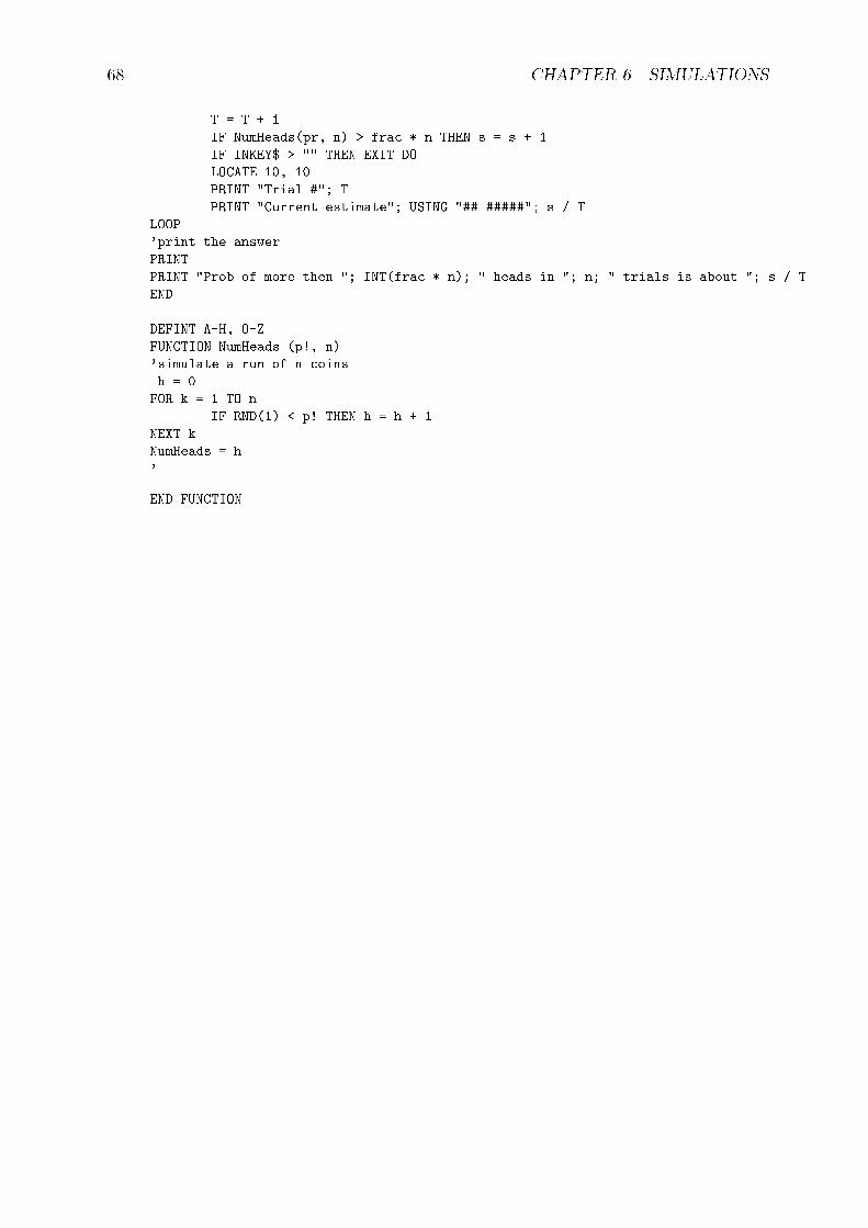
68 CHAPTER 6. SIMULATIONS
T = T + 1
IF NumHeads(pr, n) > frac * n THEN s = s + 1
IF INKEY$ > "" THEN EXIT DO
LOCATE 10, 10
PRINT "Trial #"; T
PRINT "Current estimate"; USING "##.#####"; s / T
LOOP
'print the answer
PRINT "Prob of more then "; INT(frac * n); " heads in "; n; " trials is about "; s / T
END
DEFINT A-H, O-Z
FUNCTION NumHeads (p!, n)
'simulate a run of n coins
h = 0
FOR k = 1 TO n
IF RND(1) < p! THEN h = h + 1
NEXT k
NumHeads = h
'
END FUNCTION

Chapter 7
Introduction to stochastic processes
stochastic, a. conjectural; able to conjectureWebster's New Universal Unabridged Dictionary
Stochastic processes model evolution of systems that either exhibit inherent random-ness, or operate in an unpredictable environment. This unpredictability may have morethan one form, see Section 7.3.
Probability provides models for analyzing random or unpredictable outcomes. Themain new ingredient in stochastic processes is the explicit role of time. A stochasticprocess is described by its position X(t) at time t 2 [0; 1], t 2 [0;1), or t 2 f0; 1; : : :g.
From the conceptual point of view, stochastic processes that use discrete moments oftime t 2 f0; 1; : : :g are the simplest. Since the discrete moments of time can representarbitrarily small time increments, discrete time models are rich enough to model real-worldphenomena. Continuous time versions are convenient mathematical idealizations.
7.1 Di�erence Equations
Mathematical models of time evolution of deterministic systems often involve di�erentialequations.
Di�erence equations are discrete analogues of the di�erential equations. Di�erenceequations occur in applied problems, and also when solving di�erential equations byseries expansions, or by Euler's method. The concepts of numerical versus analyticalsolution, initial values, boundary values, linearity, and superposition of solutions occur inthe discrete setup in complete analogy with the theory of di�erential equations.
A di�erence equation determines unknown sequence (yn) through a recurrence relationthat speci�es the pattern. We will consider only special cases of classes of equation
yn+1 = f(n; yn; yn�1; : : : ; yn�k+1):
Here coe�cient k is the order of the equation. For instance, yn+1 = f(n; yn) is an equationof order 1, yn+1 = f(n; yn; yn�1) is an equation of order 2, etc.
7.1.1 Examples
69

70 CHAPTER 7. INTRODUCTION TO STOCHASTIC PROCESSES
Example 7.1 Suppose a sequence yn is to satisfy
yn+1 = cos(yn); (7:1)
where the cosine function is in radians.
It is easy to write a short program that computes the values of yn. But to compute theactual sequence we need to specify the initial value y0. Table 7.1 gives sample outputs ofsuch a program for several choices of y0.
y0 y1 y2 y3 y4 y5 y6 y7 y8
-1 .5403023 .8575532 .6542898 .7934803 .7013688 .7639596 .7221025 .7504177-.5 .8775826 .6390125 .8026851 .694778 .7681958 .7191654 .7523558 .73008110 1 .5403023 .8575532 .6542898 .7934803 .7013688 .7639596 .7221025.5 .8775826 .6390125 .8026851 .694778 .7681958 .7191654 .7523558 .73008111 .5403023 .8575532 .6542898 .7934803 .7013688 .7639596 .7221025 .7504177
1.5 .0707372 .9974992 .542405 .8564697 .6551088 .7929816 .7017242 .76373032 -.4161468 .9146533 .6100653 .8196106 .6825058 .7759946 .7137247 .7559287
Table 7.1: Sequences yn satisfying equation (7.1) with di�erent initial values y0.
Similar numerical procedures show up in di�erential equations, where they are usedto approximate continuous solutions by discretizing time. The procedure is called Eulermethod, or tangent line method.
Example
Some di�erence equations are simpler than others. Suppose a sequence yn is to satisfy
yn+1 = yn + d; (7:2)
where d is a given number. It is easy to write a short program that computes values ofyn. To compute them we again need to specify the initial value y0.
On the other hand, we may notice that equation (7.2) de�nes the arithmetic progres-sion. Instead of a table like Table 7.1, we can write down the solution for all possiblevalues of y0 and for all n. Namely,
yn = y0 + dn: (7:3)
In general, an analytical solution of the di�erence equation is the formula that expressesyn as the function of n. This should be contrasted with the numerical solution which isan algorithm, or computer program, that computes values of yn. The general solution isthe function of both y0 and n, as contrasted with a particular solution that works for aprescribed initial value1 y0 only.
1Such as y0 = 0.

7.2. LINEAR DIFFERENCE EQUATIONS 71
Example 7.2 Here is another well known di�erence equation with obvious solution. Sup-pose
yn+1 = ryn; (7:4)
where r is a given number. Equation (7.4) de�nes a geometric progression and its solutionis.
yn = y0rn (7:5)
Examples 7.1.1 and 7.2 are deceptively simple. Not every di�erence equation has asimple or easy to guess answer.
Example
The following equation de�nes the Fibonacci sequence
yn+1 = yn + yn�1: (7:6)
In a typical application, yn denotes the number of rabbits at the end of the nth month.In particular, if we buy one newborn rabbit at the beginning of the �rst month then the�rst terms of the sequence are easy2 to write down:1, 1, 2, 3, 5, 8, 13, 21, : : :Without much di�culty this can be converted to a computer program and used to answerquestions likeWhen will the population of rabbits exceed 1 million? The general expression(solution) of the equation corresponding to this situation is given by the following formula.
yn =1p5
1 +
p5
2
!n
� 1p5
1�p5
2
!n
This is the outcome of the standard computation!
7.2 Linear di�erence equations
Many interesting di�erence equations, including (7.2), (7.4), (7.6) fall into the categoryof linear di�erence equations with constant coe�cients. The �rst order linear di�erenceequations with constant coe�cients has the form
yn+1 + ayn = g(n):
The second order linear di�erence equations with constant coe�cients has the form
yn+2 + ayn+1 + byn = g(n):
A method to solve di�erence equation of order 2 consists of the following steps:
2Following good mathematical practise, we simplify the real world and assume that a single mature
rabbit will produce one o�spring every month.

72 CHAPTER 7. INTRODUCTION TO STOCHASTIC PROCESSES
� First we solve the \homogeneous equation" yn+2 + ayn+1 + byn = 0. This is ac-complished through the substitution yn = rn,which leads to the characteristicequation r2 + ar + b = 0 for r. Once two roots are found, the general solu-tion is yn = C1r
n1 + C2r
n2 . The notable exception when the roots are equal is
yn = C1rn0 + C2nr
n0 .
� Secondly, we �nd any solution of the non-homogeneous equation, disregarding initialconditions. This can be accomplished by the method of varying parameters: tryyn = C1(n)r
n1 +C2(n)r
n2 . Or by guessing. In the often encountered polynomial case
g(x) = n` the trial solution yn = ns(u0 + u1n + : : :+ u`n`) will work (s = 0 except
when yn = n solves the homogeneous equation, in which case s = 1).
� In the �nal step the general solution to homogeneous equation is combined with theparticular solution to non-homogeneous equation, and the initial value problem issolved.
Example
Here is an example of the applied problem that leads to a natural, but not obviouslysolvable di�erence equation.
Suppose you borrow y0 dollars on �xed monthly interest rate r. If you do not makeany payments on your loan, then your balance will \balloon" exponentially. Formulayn = (1 + r)ny0 expresses monthly balance after n months when no loan payments aremade. Some people prefer to pay a �xed amount of p dollars at the end of each month.If p is large enough, then the balance may even shrink down! This situations is easilydescribed by a di�erence equation. To write it down, compute the next month balance,if the previous month balance is known:
yn+1 = (1 + r)yn � p: (7:7)
Equation (7.7) and its general solution are of interest to bank o�cers and to their cus-tomers. From the formula for yn, they can determine monthly payments that will pay aloan o� in the prescribed amount of time.
In di�erential equations, we often solve a similar problem in continuous time, withcontinuous compounding and continuous payments schedule. This is a mathematicalsimpli�cation of the actual banking situation, but the answers are reasonably close, andthey are easier to get.
Here is an example of the mathematical problem that leads to a natural, but non-trivial3 di�erence equation.
Example 7.3 Suppose we want to �nd the formula for the sum of all consecutive integersfrom 1 to n. Let the answer by yn. Then the recurrence formula
yn+1 = yn + n + 1 (7:8)
holds.
3Most likely, you know the solution to this one, but the method is useful for other problems as well.
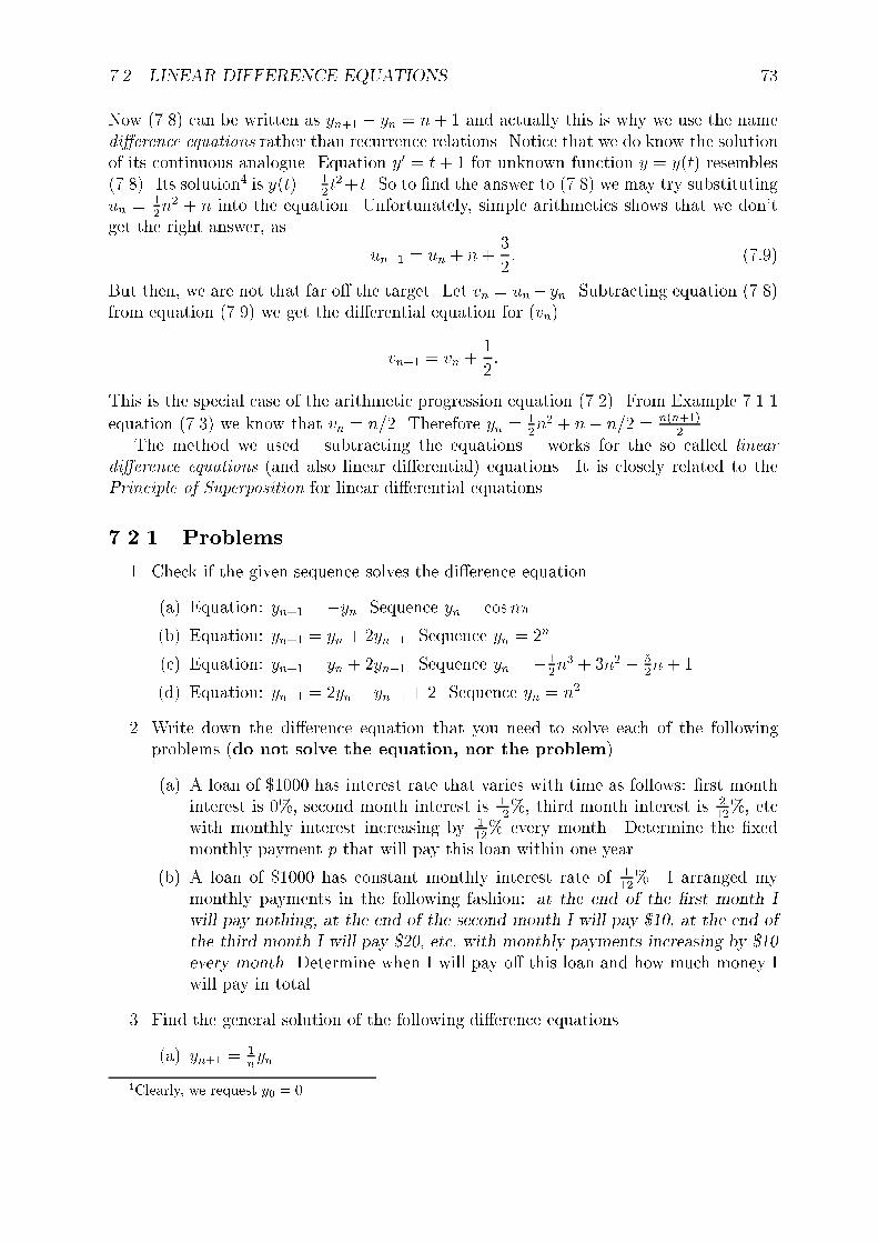
7.2. LINEAR DIFFERENCE EQUATIONS 73
Now (7.8) can be written as yn+1 � yn = n+ 1 and actually this is why we use the namedi�erence equations rather than recurrence relations. Notice that we do know the solutionof its continuous analogue. Equation y0 = t+ 1 for unknown function y = y(t) resembles(7.8). Its solution4 is y(t) = 1
2t2+t. So to �nd the answer to (7.8) we may try substituting
un = 12n2 + n into the equation. Unfortunately, simple arithmetics shows that we don't
get the right answer, as
un+1 = un + n+3
2: (7:9)
But then, we are not that far o� the target. Let vn = un� yn. Subtracting equation (7.8)from equation (7.9) we get the di�erential equation for (vn)
vn+1 = vn +1
2:
This is the special case of the arithmetic progression equation (7.2). From Example 7.1.1
equation (7.3) we know that vn = n=2. Therefore yn =12n2 + n� n=2 = n(n+1)
2
The method we used { subtracting the equations { works for the so called lineardi�erence equations (and also linear di�erential) equations. It is closely related to thePrinciple of Superposition for linear di�erential equations.
7.2.1 Problems
1. Check if the given sequence solves the di�erence equation.
(a) Equation: yn+1 = �yn. Sequence yn = cosn�.
(b) Equation: yn+1 = yn + 2yn�1. Sequence yn = 2n.
(c) Equation: yn+1 = yn + 2yn�1. Sequence yn = �12n3 + 3n2 � 5
2n+ 1.
(d) Equation: yn+1 = 2yn � yn�1 + 2. Sequence yn = n2.
2. Write down the di�erence equation that you need to solve each of the followingproblems (do not solve the equation, nor the problem).
(a) A loan of $1000 has interest rate that varies with time as follows: �rst monthinterest is 0%, second month interest is 1
12%, third month interest is 2
12%, etc
with monthly interest increasing by 112% every month. Determine the �xed
monthly payment p that will pay this loan within one year.
(b) A loan of $1000 has constant monthly interest rate of 112%. I arranged my
monthly payments in the following fashion: at the end of the �rst month Iwill pay nothing, at the end of the second month I will pay $10, at the end ofthe third month I will pay $20, etc, with monthly payments increasing by $10every month. Determine when I will pay o� this loan and how much money Iwill pay in total.
3. Find the general solution of the following di�erence equations.
(a) yn+1 =1nyn
4Clearly, we request y0 = 0.

74 CHAPTER 7. INTRODUCTION TO STOCHASTIC PROCESSES
(b) yn+1 =n
n+1yn
(c) n(n + 1)yn+1 = yn
4. Solve the given initial value problem for the di�erence equation.
(a) yn+1 =1nyn; y0=1
(b) yn+1 =n
n+1yn�1 ; y0 = 1; y1 = 0
(c) n(n + 1)yn+1 = 2yn ;y0 = 1; y1 = 0
5. Find the formula for
(a) yn = 12 + 22 + : : :+ n2
(b) yn = 13 + 23 + : : :+ n3
(c) yn =12+ 1
6+ : : :+ 1
n(n+1)
(d) yn = 1 + r + r2 + : : :+ rn�1
(e) yn = r + 2r2 + 3r3 + : : :+ nrn
6. Each solution of equation (7.1) has the limit limn!1 yn. Show that the �rst digitsof this limit are :739085133.
7.3 Recursive equations, chaos, randomness
Before jumping to models that use explicit randomness in their evolution, it is quiteilluminating to analyze �rst some mathematically simple and well de�ned \deterministicevolutionary processes". The following set of examples describes deterministic evolutionin discrete time of a system described by a single numerical parameter x 2 (0; 1). All ofthe examples fall into the category of (non-linear) di�erence equations: given initial valuex0 2 (0; 1) and a simple evolution equation of the form xn+1 = g(xn), we are supposed tomake inferences about the behavior of the solutions.
There is no randomness in the evolution itself. But since we are allowed to chooseany initial condition, and no initial condition can be measured exactly, we may as wellconsider the initial value to be random.
Example 7.4 Equationxn+1 = cos(xn)
is analyzed numerically in Example 7.1. A useful technique to analyze such equations is tograph function y = g(x) together with line y = x, and represent the sequence xk by points(xk; xk) on the line. The actual proof that xn ! x� may perhaps be not that obvious, butthe geometric argument seems to be quite convincing.
Example 7.5 Let fxg denote the fractional part of x. Equation
xn+1 = f2xnguses discontinuous function g(x). The previous graphical technique is more di�cult toapply here, but the reason for this di�culty might be not apparent. Special initial points,

7.3. RECURSIVE EQUATIONS, CHAOS, RANDOMNESS 75
like x0 = 1=2; x0 = 1=4; x0 = 1=8; x0 = 3=4; : : : are relatively easy to analyze. But theseare exceptional - the majority of the initial points actually doesn't follow this pattern.
Here is a rather surprising fact. Suppose x0 is selected at random. Since xk is afunction of x0, and x0 is random, xk becomes a random variable. It may happen thatxk < 1=2. Call this event Ak. The reasoning presented in Section 6.1.1 implies thatevents fAkg are independent and have the same probability Pr(Ak) = 1=2. Therefore thedeterministic evolution equation contains at least as much randomness as the tosses of acoin.
The last example may perhaps give the impression that it is the discontinuity of theevolution equation that is the source of di�culties. This is not at all the case.
Example 7.6 Equationxn+1 = 4xn(1� xn)
is another example of the "chaotic equation" with solutions exhibiting as much irregularityas the tosses of a coin. Attempts at graphing its solutions do no indicate any patterns.Tiny di�erences in the choice of initial value x0 signi�cantly change the evolution withinshort time.
Example 7.6 indicates that \naive" prediction of the future of a system is unreliableeven within the realm of deterministic evolution equations.
On the other hand, there are aspects of the evolution that we can analyze reliably.These deal with the average behavior of the evolution.
There are two classes of questions that we can answer, but both deal with statisticalnature of the evolution:
� what happens if the same experiment is repeated many times (with slightly di�erentinitial conditions)?
� What is the average behavior of the system over long periods of time?
For instance, we can ask and get reliable answers to questions like:
� What is the average 1n
Pnj=1 xj?
� What is 1n
Pnj=1 U(xj) for a given function U?
� How often xj < 1=2? (Meaning - what proportion of j � T satis�es the conditionfor large T .)
� How often x3 < 1=2 when x0 is selected according to density g(x)? (Meaning - whatproportion of x0 satis�es the condition for large number of initial points x0.)
Theory of stochastic processes uses descriptive rather than casual models. Its primarygoal is to isolate methods that answer questions that can be answered - about the averagesand chances of events. It is setup in the form that makes it more natural to ask the"correct" questions. But in real life, and in simulations, we do have access to aspectsof the phenomenon than what the theory does not expose. In analyzing simulationsit is important to keep in mind the examples above. Avoid collecting data that dealwith instances rather than statistical phenomena. Print out well de�ned statistics of thesimulation only. Do not clutter your simulations with irrelevant details.

76 CHAPTER 7. INTRODUCTION TO STOCHASTIC PROCESSES
7.4 Modeling and simulation
The quick way to get insights into operation of real systems is to model their behavior.Here are examples of enterprises that operate under randomness. Mathematicians devisedmethods of modelling each of these. But it is interesting also to simulate their behavior.Notice that simulations require assumptions, but so do the analytical methods. Regardlessof the method, we have to be careful about what are the questions we can answer.
Example 7.7 Suppose we want to study how much capital is needed to run a casino. Weneed to answer the following.
� How often do people win?
� How likely is the casino to loose money in a day? In a month?
� How much capital should be kept on hand to cover the losses?
There is also a number of questions that we do not want to answer.
Example 7.8 Suppose we want to study how much capital is needed to insure cars. Weneed to answer the following.
� How often do accidents occur? How expensive are repairs/medical costs?
� How likely is that the insurance company looses money in a day? In a month?
� How much capital should be kept on hand to cover losses?
There is also a number of questions that we do not want to answer. For instance we donot want to predict whether I'll �le an insurance claim today, driving back home on I-74without enough sleep since I was preparing this class until 3AM.
Example 7.9 A construction company has n jobs to be performed in the future. Foreach of these jobs, experts provide estimate of the cost. Then, after questioning, theycomplement the estimates by the lower/upper bound for the costs. How much moneyshould be allotted?
Example 7.10 A store averages �(t) customers per hour at time t of the day. Eachcustomer brings some (random) pro�t. However, a customer may just leave the storewithout shopping, if the lines are too long.
� How many cashiers should be available for each shift (time) t?
� What are the pro�ts on average?
7.5 Random walks
A random walk is a process of the form Xn =Pn
j=1 �j, where �j are i. i. d. Random walkshave independent increments , and describe the accumulation of independent contributionsover time.
Random walks are examples of Markov processes which will be studied in detail inChapter 8. Their special structure allows to analyze them independently of the generaltheory.
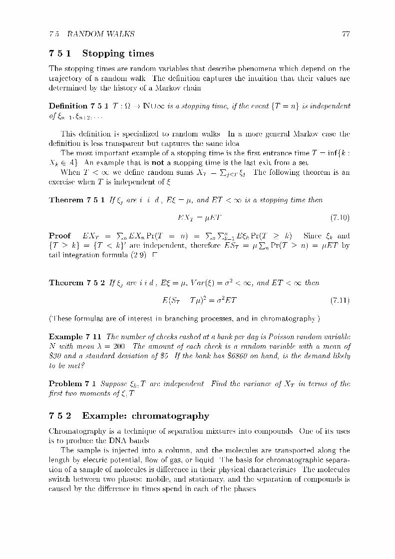
7.5. RANDOM WALKS 77
7.5.1 Stopping times
The stopping times are random variables that describe phenomena which depend on thetrajectory of a random walk. The de�nition captures the intuition that their values aredetermined by the history of a Markov chain.
De�nition 7.5.1 T : ! IN[1 is a stopping time, if the event fT = ng is independentof �n+1; �n+2; : : :.
This de�nition is specialized to random walks. In a more general Markov case thede�nition is less transparent but captures the same idea.
The most important example of a stopping time is the �rst entrance time T = inffk :Xk 2 Ag. An example that is not a stopping time is the last exit from a set.
When T < 1 we de�ne random sums XT =P
j�T �j. The following theorem is anexercise when T is independent of �.
Theorem 7.5.1 If �j are i. i. d., E� = �, and ET <1 is a stopping time then
EXT = �ET (7:10)
Proof. EXT =P
nEXn Pr(T = n) =P
n
Pnk=1E�k Pr(T � k). Since �k and
fT � kg = fT < kg0 are independent, therefore EST = �P
n Pr(T � n) = �ET bytail integration formula (2.9). 2
Theorem 7.5.2 If �j are i.i.d., E� = �, V ar(�) = �2 <1, and ET <1 then
E(ST � T�)2 = �2ET (7:11)
(These formulas are of interest in branching processes, and in chromatography.)
Example 7.11 The number of checks cashed at a bank per day is Poisson random variableN with mean � = 200. The amount of each check is a random variable with a mean of$30 and a standard deviation of $5. If the bank has $6860 on hand, is the demand likelyto be met?
Problem 7.1 Suppose �k; T are independent. Find the variance of XT in terms of the�rst two moments of �; T .
7.5.2 Example: chromatography
Chromatography is a technique of separation mixtures into compounds. One of its usesis to produce the DNA bands.
The sample is injected into a column, and the molecules are transported along thelength by electric potential, ow of gas, or liquid. The basis for chromatographic separa-tion of a sample of molecules is di�erence in their physical characteristics. The moleculesswitch between two phases: mobile, and stationary, and the separation of compounds iscaused by the di�erence in times spend in each of the phases.

78 CHAPTER 7. INTRODUCTION TO STOCHASTIC PROCESSES
Suppose that the molecules of a compound spend random independent amounts oftime Uk in mobile phase and random amount of time Wk in the stationary phase. Thusat time t the position of a molecule is given by a random sum v
PT (t)j=1 Uj, where T (t) =
inffk : Pkj=1 Uj +Wj > tg.
Section 7.5.1 gives formulas for the mean and the variance of the position. Since thenumber of transitions T is likely to be large for a typical molecule, it isn't surprising thatthe actual position has (asymptotically) normal distribution. (The actual Central LimitTheorem for random sums is not stated in these notes.)
Exercise 7.2 Simulate the output of the chromatography column of �xed length separat-ing a pair of substances that have di�erent distributions of mobile and stationary phasesUk;Wk. Select a hundred particles of each substance, and measure the degree of separationat the end of the column.
7.5.3 Ruining a gambler
The following model is a reasonable approximation to some of the examples in Section7.4.
Suppose a gambler can a�ord to loose amount L > 0, while the casino has capitalC < 0. Let �j = �1 be i. i. d. random variables modelling the outcomes of consecutivegames, Sn be the partial sums (representing gains of the gambler), and let T = inffk :Sk � L or Sk � Cg be the total number of games played. Then Pr(T > k) = Pr(C <Sk < L) and thus ET =
Pk Pr(C < Sk < L).
The special case Pr(� = �1) = 1=2 is easily solved, since in this case EST = E�ET =0. Let p = Pr(ST = C) denote the probability of ruining the casino. Since ST is either C,or L we have 0 = EST = pC + (1� p)L, giving p = L=(L�C). This formula means thata gambler has a fair chance of ruining a casino in a fair game, provided he brings withhim enough cash L.
For more general random walks (and less fair games) probability of gambler's ruin canbe found explicitly using the one-step-analysis (Section 8.3). It is also interesting to �ndhow long a game like that would last on average. (The expression for ET given above isnot explicit.)
7.5.4 Random growth model
The following models various growth phenomena like the spread of a disease, where theinfected individual may either die, or infect a number of other individuals. Here we con-centrate on bacteria which have simple reproduction mechanism, and all spatial relationsare neglected.
Let Xt denote the number of bacteria in t-th generation, with X0 = 1. Assume that abacteria can die with probability q > 0, or divide into two cells with probability p = 1�q,and that all deaths occur independently. Our goal here is to �nd the average number ofbacteria m(t) = E(Xt) in the t-th generation. This can be recovered from Theorem 7.5.1.Instead, we show another method based on conditioning.
The number of bacteria in the next generation is determined by binomial probabilities:Pr(Xt+1 = 2kjXt = n) = (nk)p
kqn�k. Therefore E(Xt+1jXt) = 2pXt and the average

7.5. RANDOM WALKS 79
population size m(t) = E(Xt) satis�es di�erence equation m(t + 1) = 2pm(t). We havem(t) = (2p)t. In particular, the population on average grows exponentially when p > 1=2.
It is perhaps surprising that a population of bacteria with p = 3=4, which on averagegrows by 50% per generation, has still a 1
3chance of going extinct. One way to interpret
this is to say that infections by a \deadly" and rapidly developing desease may still havea large survival rate without any intervention of medicine, or immune system. (Themethods to compute such probabilities will be introduced in Section 8.3. The answerabove assumes infection by a single cell.)
Problem 7.3 Find the formula for the variance V ar(Xt) of the number of bacteria int-th generation.
Problem 7.4 What is the probability that an infection by 10 identical bacteria with thedoubling probability p = 3=4 dies out?

80 CHAPTER 7. INTRODUCTION TO STOCHASTIC PROCESSES
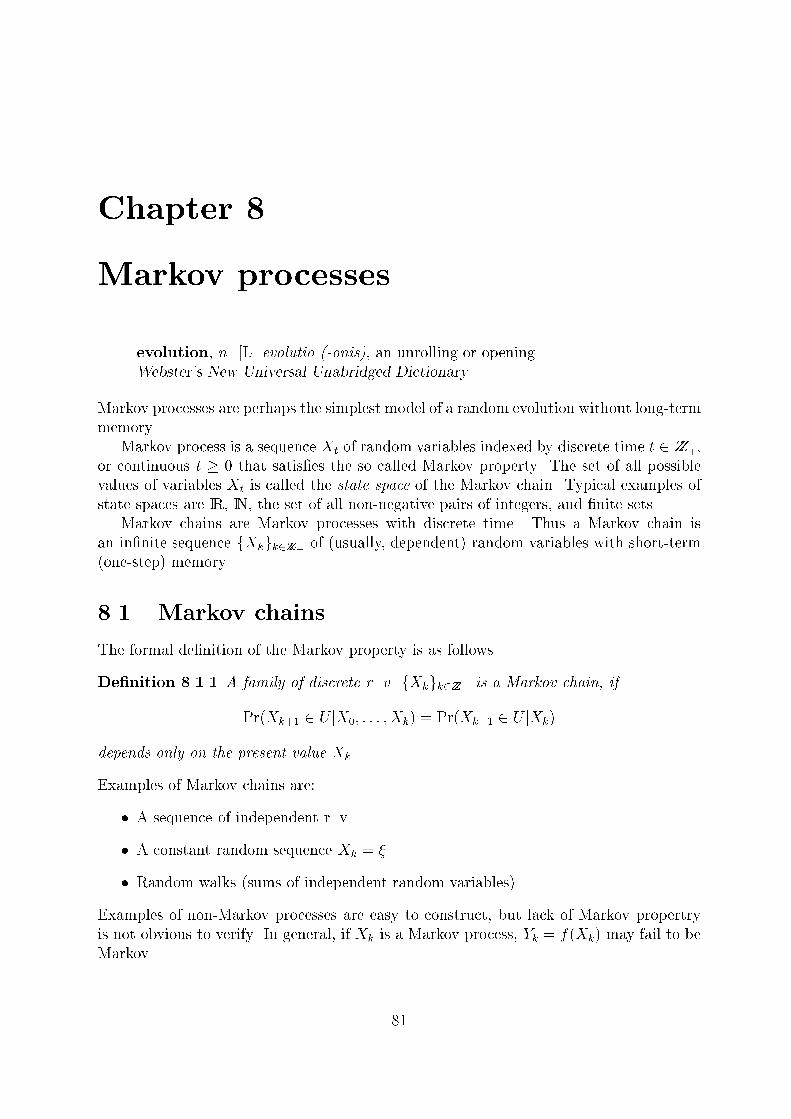
Chapter 8
Markov processes
evolution, n. [L. evolutio (-onis), an unrolling or opening...Webster's New Universal Unabridged Dictionary
Markov processes are perhaps the simplest model of a random evolution without long-termmemory.
Markov process is a sequence Xt of random variables indexed by discrete time t 2 ZZ+,or continuous t � 0 that satis�es the so called Markov property. The set of all possiblevalues of variables Xt is called the state space of the Markov chain. Typical examples ofstate spaces are IR, IN, the set of all non-negative pairs of integers, and �nite sets.
Markov chains are Markov processes with discrete time. Thus a Markov chain isan in�nite sequence fXkgk2ZZ+ of (usually, dependent) random variables with short-term(one-step) memory.
8.1 Markov chains
The formal de�nition of the Markov property is as follows.
De�nition 8.1.1 A family of discrete r. v. fXkgk2ZZ+ is a Markov chain, if
Pr(Xk+1 2 U jX0; : : : ; Xk) = Pr(Xk+1 2 U jXk)
depends only on the present value Xk.
Examples of Markov chains are:
� A sequence of independent r. v.
� A constant random sequence Xk = �.
� Random walks (sums of independent random variables).
Examples of non-Markov processes are easy to construct, but lack of Markov propertryis not obvious to verify. In general, if Xk is a Markov process, Yk = f(Xk) may fail to beMarkov.
81

82 CHAPTER 8. MARKOV PROCESSES
8.1.1 Finite state space
If a Markov chain has a �nite state space, we can always assume1 it consists of integers.Markov condition
Pr(Xk+1 = xjX0; : : : ; Xk) = Pr(Xk+1 = xjXk) (8:1)
implies that probability of reaching x in the next step depends only on the present valueXk. The probabilistic behavior of such a chain is completely determined by the initialdistribution pk = Pr(X0 = k) and the transition matrices Pn(i; j) = Pr(Xn = jjXn�1 = i),see formula (1.11) on page 15. For mathematical convenience we shall assume that onestep transition matrices Pt = P do not depend on time t. Such Markov chains are calledhomogeneous. This assumption isn't realistic, nor always convenient. For instance, theMarkov simulation in Section 8.5 uses a Markov chain with transitions that vary withtime. But homogeneous Markov chains are still exible enough to handle some timedependencies e�ciently through modi�cations to the state space.
Example 8.1 Suppose Xn is a Markov chain with periodic transition probabilities Pn =Pn+T . Then Yn = (Xn+1; Xn+2; : : : ; Xn+T ) is a homogeneous Markov chain.
Problem 8.1 Suppose �j are independent f0; 1g-valued with Pr(� = 1) = p. Let Xn =a�n + b�n+1, where ab 6= 0.
Explain why Xn is a Markov chain.Write the transition matrix for the Markov chain Xn.
Proposition 8.1.1 The probabilities Pr(Xn = jjX0 = i) are given by the i; j-entries ofthe matrix P n
Proof. This is the consequence of Markov property (8.1) and the total probability for-mula (1.10). 2
Powers of moderately sized matrices are easy to compute on the computer. SectionB.9 indicates a mathematical method of computing P n for small dimensions using theCayley-Hamilton theorem. Under certain conditions the powers converge.
Exercise 8.2 Find limn!1 P n for the matrix from Problem 8.1.
Stationary Markov processes
Suppose Pr(X0 = k) = pk, where pk solve stationarity equationsXk
pk = 1 (8.2)
[p1; : : : ; pd] = [p1; : : : ; pd]� P (8.3)
(8.4)
1Notice that this is a mathematical simpli�cation that might be not worth pursuing if the actual statespace has some convenient interpretation.

8.1. MARKOV CHAINS 83
Then the resulting process is stationary: the distribution of each k-tuple(X(t1); : : : ; X(tk)) is invariant under shifts in time, (X(t1 + s); : : : ; X(tk + s)) �=(X(t1); : : : ; X(tk)). This is interpreted as \equilibrium", or \steady state". Notice that\steady state" is a statistical concept, and is not easily visible in a simulation of thesingle trajectory. In order to be able to see it, one has to simulate a large number ofindependently evolving Markov chains that begin with the same initial distribution andhave the same transition matrix.
If Xt is a stationary Markov process and f is a function on its state space, thenY (t) = f(Xt) is also stationary, although not necessarily Markov.
If Xj(t) are independent realizations of the same Markov process and f is a function ontheir state space then Yn(t) = n�1=2
Pnj=1(f(Xj(t))� �) is stationary and approximately
normal random sequence.
8.1.2 Markov processes and graphs
The states of a Markov chain may be represented by vertices of a graph, and one steptransitions may be described by directed edges with weights. Such representation of amarkov chain aids in visualizing a Markov chain.
Classi�cation of states
Graph notions have bearing on properties of the Markov chain. In particular, Markovchain is irreducible, if the corresponding graph is connected. Markov chain is periodic, ifthere is N > 1 (the period) such that all cycles of the graph are multiples of N . If thereis no such N then Markov chain is called aperiodic.
Finite state Markov chain is regular, if there is deterministic number N such that allstates are connected by paths of length at most N .
Problem 8.3 Show that regular Markov chain is aperiodic and irreducible.
Trajectory averages
Additive functionals of a Markov process are expressions of the form 1n
Pn�1j=0 f(Xj). Under
certain conditions, the averages converge and the limit doesn't depend on the initialdistribution. Under certain conditions, partial sums are approximately normal.
Problem 8.4 Let Xk be an irreducible f0; 1g-valued Markov chain with invariant initialdistribution.
� Show that there is C > 0 such V ar(PT
t=0Xt) � CT .
� Use the above to show that the law of large numbers holds.

84 CHAPTER 8. MARKOV PROCESSES
Asymptotic probabilities
Let pk(n) = Pr(Xn = k), and suppose that the limit pk(1) = limn!1 pk(n) exists. Sincepk(n + 1) =
Pdj=1 pj(n)P (j; k), therefore the limit probabilities satisfy the stationarity
equations (8.2)For regular (�nite state space) Markov chains the limit actually exists independently
of the initial state. Therefore the stationarity equations can be used to �nd the limit.
Problem 8.5 Let P =
"1=4 3=43=4 1=4
#.
� Find the initial distribution of X0 that results in a stationary process.
� Find the limiting distribution limn!1 pk(n).
Problem 8.6 Let P =
"0 11 0
#.
� Find the initial distribution of X0 that results in a stationary process.
� Explain why limn!1 pk(n) does not exist.
Problem 8.7 Let P =
"1 00 1
#.
� Find the initial distribution of X0 that results in a stationary process.
� Find the limiting distribution limn!1 pk(n).
Example: two-state Markov chain
Suppose Xk is a Markov chain with transition matrix P =
"1� a ab 1� b
#. Then
P n =1
a+ b
"b ab a
#+(1� a� b)n
a+ b
"a �a�b b
#:
If 0 < a; b < 1
P n !"
ba+b
aa+b
ba+b
aa+b
#
and the rate of convergence is exponentially fast.
Problem 8.8 Suppose Xk is a Markov chain with transition matrix P =
"a 1� a
1� b b
#.
Then Yn = (Xn; Xn+1) is also a Markov process. Find its transition matrix and the sta-tionary distribution.

8.2. SIMULATING MARKOV CHAINS 85
8.2 Simulating Markov chains
Homogeneous and non-homogeneous Markov chains with �nite state space are fairlystraightforward to simulate. A generic prescription is to simulate Xn+1 using the condi-tional distribution determined by Xn. This simulation di�ers very little from the genericmethod described in Section 2.1.2
Example: how long a committee should discuss a topic?
This example involves simulation of a Markov chain. For Markov chains many theoreticalresults are available, but simulation is often the most expedient way to study it.
Exercise 8.9 Suppose n people on a committee discuss a certain issue. When one person�nishes speaking, we assume that it is equally likely that any of the other n � 1 begins.We also assume that each person speaks for exponentially distributed random time. Howlong does it take on average for all participants to take part in the discussion?
8.2.1 Example: soccer
The soccer game2 is played by two teams, each with 10 players in the �eld and a goalkeeper.A modern line-up split the players into between the zones of defence, center, and attack.Thus a con�guration (3-4-4) means 3 defenders (backs), 4 mid�eld link men and 4 strikers(forwards). In the Markov model of soccer we will just watch the position of the ball, andwe assume it can be only in one of the �ve positions: left goal, left defence, mid�eld, rightdefence, right goal. Wee shall assume that at every unit of time the ball has to move leftor right with chances proportional to the number of players lined-up for a given position.
For each possible con�gurations of teams, we could determine the average score, andthus determine which player distribution is the best, if there is one. If there is no bestsingle arrangement that wins against all other arrangements, then we should still be ableto �nd the optimal mixed strategy.
Exercise 8.10 For the Markov chain de�ned above, select a pair of con�gurations anddetermine the following.
� Average time to hit the goal
� Probability of scoring left before right goal
� Long run behavior of the ball.
2Source: football in A. Hornby, Oxford Advanced Learner's Dictionary of Current English , OxfordUniversity Press 1974
86 CHAPTER 8. MARKOV PROCESSES
A brief review of game theory
In game theory, a rational player is supposed to minimize her losses against the best choiceof the opponent. The terminology uses minimax= minimize maximal loss, maximin=maximize minimal gain; the amazing fact is that these are equal and often the optimalstrategies are randomized (mixed).
The optimal strategy in a game is the best (in the above minimax sense) randomizedstrategy against every deterministic strategy of the opponent.
Problem 8.11 What is the \optimal" arrangement of players in soccer?
Modi�cations
As given above, the model of the soccer game is simple enough to be analyzed withoutcomputer. In a more realistic model one could consider additional factors.
� The �eld can be partitioned into more pieces
� The �eld is a two-dimensional rectangle.
� Players can move between neighboring portions of the game �eld.
� Players react to the position of the ball
� Players react to the positions of other players
� Some soccer players are more skilled.
8.3 One step analysis
For homogeneous Markov chains a surprising number of quantities of interest can becomputed using the so called one step analysis. The idea is to �nd out what happens tothe quantity of interest within one step of the evolution, and solve the resulting di�erenceequation.
Example 8.2 In the setup of Section 7.5.3, suppose Pr(� = 1) = p = 1 � Pr(� = �1).Let T be the �rst time random walk reaches L > 0 or C < 0. Find the probability ofwinning (ruining the casino) Pr(XT = CjX0 = 0).
Note that evven though we are interested in a single number Pr(XT = CjX0 = 0),the �st-step analysis requires computing probabilities p(x) = Pr(XT = CjX0 = x) for allinitial positions x.
Example 8.3 Suppose Pr(� = 1) = p;Pr(� = �1)1� p. Let T be the �rst time randomwalk reaches L > 0 or C < 0. Find the average length of the game E0(T ).
Note that the �st-step analysis requires computing m(x) = Ex(T ) for all initial posi-tions x.
Problem 8.12 On average, how long does it take for a symmetric random walk on asquare lattice to exit from a d� d square?
8.3. ONE STEP ANALYSIS 87
Problem 8.13 For the Markov chain de�ned in Section 8.2.1, select a pair of playercon�gurations and determine the following.
� Average time to hit the goal
� Probability of scoring left before right goal
� Long run behavior of the ball.
Problem 8.14 A fair coin is tossed repeatedly until k = 2 successive heads appear. Whatis the average number of tosses required? (Hint: see Problem 8.1, or run a simulation.)
Problem 8.15 One of the quality control rules is to stop the process when on k = 8successive days the process runs above, or below, speci�cation line. On average, how oftena process that does not need any adjustment will be stopped by this rule?
8.3.1 Example: vehicle insurance claims
Suppose that you have an insurance contract for a vehicle. The premium payment is dueyearly in advance and there are four levels P1 > P2 > P3 > P4. The basic premium is P1,unless no claims were made in the previous year. If no claims were made in a given year,then the premium for the following year is upgraded to the next category.
Suppose that the probability of the damage larger than s hundred dollars is e�s (sub-stitute your favorite density for the exponential density used in this example). Becauseof the incentive of lowered premium, not all damage should be reported. The goal of thisexample is to determine numbers s1; s2; s3; s4 above which the claims should be �led; sjis a cuto� used in a year when premium Pj is paid.
Let Xt be the type of premium paid in t-th year. Clearly, the transitions are i 7! 1with probability e�si, 1 7! 2 with probability 1� e�s1, etc.
In the long run, the yearly cost is
C(s1; s2; s3; s4) =X
�j(Pj +mj); (8:5)
where �j are the equilibrium probabilities and mj are average un-reimbursed costs: mj =100
R sj0 se�s ds. The optimal claim limits follow by minimizing expression (8.5).
Exercise 8.16 Find optimal sj when P1 = 800; P2 = 720; P3 = 650; P4 = 600 (about 10%discount).
8.3.2 Example: a game of piggy
In a game of piggy, each player tosses two dice, and has an option of adding the outcometo his score, or rolling again. The game ends when the �rst player exceeds 100 points.
Each player has to toss the dice at least once per turn. The player can choose to tossthe dice as many times as (s)he wishes as long as no ace occurs. However the currenttotal is added to player's score only when the player ends his turn voluntarily.

88 CHAPTER 8. MARKOV PROCESSES
If an ace occurs, then the player's turn is over, and his score is not increased. If twoaces occur then the score is set to zero.
A player chooses the following strategy: toss the dice for as long as an ace occurs, orthe sum of current subtotal+score exceeds number K. (If her score exceeds K she tossesthe dice once, as this is required by the rules.) The quantity to optimize is the averagenumber of turns that takes the player to reach the score of a hundred. The number ofturns under this strategy is the number of aces when the score is less than K, plus thenumber of throws when the score is larger than K.
If Xk denotes players score after the k-th throw, then clearly Xk is a Markov chainwith the �nite number of states, and with chance 1
36of returning to zero at each turn.
Which value of K minimizes the average number of turns that takes the player toreach a hundred?
A simple-minded computation would just take into account the average gain anddisregard the score completely. If the players subtotal is t then after the additional throwthe total is on average 23=36 � (t + 7). This is less then t for t � 12, thus there is nopoint continuing beyond 12. Is this conclusion correct? Should the player choose to stoponce the total on the dice exceeds 12?
Exercise 8.17 What is the average number of turns it takes to reach a 100 under thisstrategy?
A less simple-minded computation would take into account the average gain: If theplayers score is s then after the additional throw his score on average is 1=36� 0+ 1=3�s+23=36� (s+7) which is more then s for s < 7�23. Is this conclusion correct? Shouldthe player always choose to toss again?
Exercise 8.18 What is the average number of turns it takes to reach a 100 under thisstrategy?
Exercise 8.19 What is the average number of turns it takes to reach a 100 under thecautious strategy of no additional tosses?
Another computation would take into account the current score s and current subtotalt. After the additional throw the numbers on average are s1 = 1=36 � 0 + 35=36 � s,t1 = 23=36� (t + 7). On average, t1 + s1 > t + s when t < 12� s=13.
More complicated strategies could depend on current totals of other players, currentscore of the player, and the subtotal in some more complicated fashion. For instance, if sdenotes the score, t denotes current subtotal, one could stop using two-parameter criteriont > A� Bs. This may have seemingly di�erent e�ects than the previous strategy: whenA is large, and score s is close to 0 there is no need for stopping; but if accumulated scores is large, the player may behave more cautiously.
One could optimize the probability of winning against k = 3; 4 players instead of justminimizing the average number of tosses. The latter puts this problem into game theoryframework. Simulations seem to indicate that the strategy based on t < 25 � 1
9s works
well against inexperienced human players.

8.4. RECURRENCE 89
8.4 Recurrence
A state x of Markov chain is recurrent, if with probability one the chain returns back tox. Otherwise it is called transient. If Xt is irreducible then all states are simultaneouslyeither recurrent, or transient.
Theorem 8.4.1 State x is recurrent i�PPx;x(t) =1.
Proof. Let M be the number of times Xt returns to state x.Let f be the probability of returning to x. State x is recurrent i� f = 1. Suppose
f < 1 and let M be the number of returns. Clearly Prx(M � k) = fk, thus Ex(M) =f=(1� f) <1. Since M =
Pt IfXt=xg, Ex(M) =
PPx;x(t).
2
Interesting fact: simple random walks in Rd are recurrent when d < 3, transient whend � 3. However the return times have in�nite average.
Theorem 8.4.2 Let T be a return time, and suppose m(x) = ExT <1. Then Px;x(t)!1=m(x) as t!1.
Problem 8.20 Suppose Markov chain Xt moves to the right k 7! k + 1 with probability1=k or returns to 1 with probability 1 � 1
k, k = 1; 2; : : :. Find its stationary distribution,
and the average return time to state k.
8.5 Simulated annealing
This sections describes a more re�ned method for randomized search of minima of func-tions.
Suppose a �nite set V is given, and we are to minimize a function U : V ! IR.
The �rst step of design is to specify a connected directed graph G = (V;E). In otherwords, for every point u 2 V we need to pick the set of directed edges (u; v) for themarkov chain to follow from state u. (This step is usually performed for computa-tional e�ciency; theoretically, all possible transitions could be admissible.)
The second step is to choose "control parameter" � that will vary as the program isrunning.
The third step is to de�ne transition probabilities:
P (u; v) = C(u)e��(U(v)�U(u))+ ; (8:6)
where C(u; v) =P
v e��(U(v)�U(u))+ is the norming constant, and the only v's con-
sidered are those with (u; v) 2 E. (Can you explain now why G shouldn't be thecomplete graph).
90 CHAPTER 8. MARKOV PROCESSES
Theorem 8.5.1 The invariant measure of transition matrix (8.6) is p�(u) =1Ze�U(u)
Proof. To check the invariance condition, denote N (u) = fv : (u; v) 2 Eg.2
An e�cient realization of the above is to pick v 2 Nu at random and accept it with
probability
(1 if U(v) � U(u)e��U(v) otherwise.
8.5.1 Program listing
The program is available online, or on the disk.
8.6 Solving di�erence equations through simula-
tions
In the example below we limit our attention to the one-dimensional problem. This sim-pli�es the notation, while the basic ideas are the same.
Let u(x; t) be an unknown function of x 2 IRd; t � 0. The di�erence equation we maywant to solve is the following discrete analog of the di�usion equation.
u(x; t+ 1) = u(x; t) + A1
2dX
v=�eku(x+ v; t) (8.7)
u(x; o) = u0(x) (8.8)
The solution is u(x; t) = E(u0(St)), where St =P
j�t �j is the sum of independent
random variables with 2d equally likely values �ek 2 IRd.
8.7 Markov Autoregressive processes
Suppose �k is a stationary Markov chain and let Xn be the solution of the di�erenceequation Xn+1� aXn = �n+1. One can write the transition Matrix for Markov process Xt
and try �nd the stationary distribution for X0.A more direct method is based on the fact that the solution of the di�erence equation
is Xt = atX0 + at�1�1 + : : : + a�t�1 + �t. Therefore if jaj < 1, the stationary initialdistribution is X0 =
Pak�k. Thus Xt =
P1k=0 a
k�t�k
Problem 8.21 Suppose �k are i. i. d. Find the covariance EX0Xk.
Problem 8.22 Suppose �k are i. i. d. Find E(XkjX0).
Solutions of higher order di�erence equations can be easily out into the Markov frame-work, too. If Xn+2 + aXn+1 + bXn = �n+1 then Yn = (Xn+1; Xn) is Markov and satis�esthe corresponding equation in matrix form: Yn+1 = AYn+�n+1. Therefore the stationarysolution exist provided that the eigenvalues of A satisfy inequality j�jj < 1.
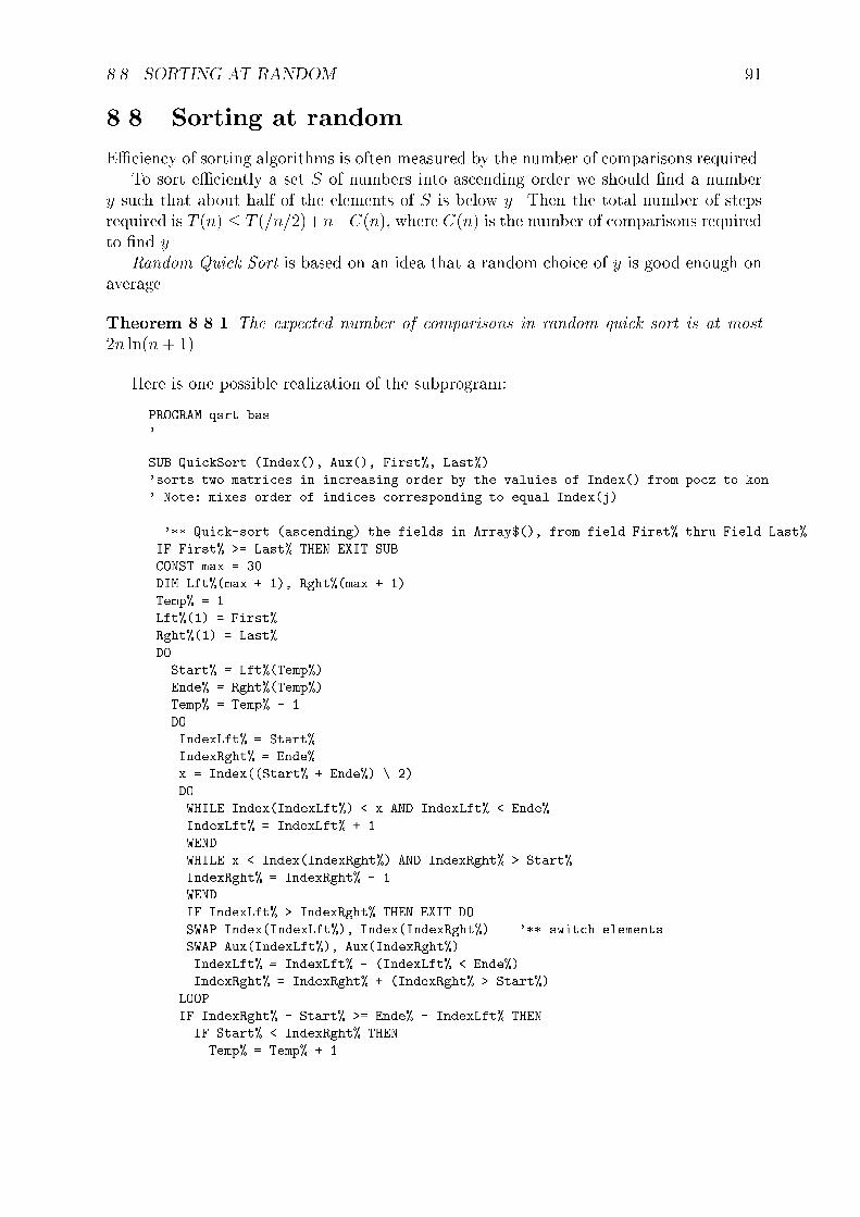
8.8. SORTING AT RANDOM 91
8.8 Sorting at random
E�ciency of sorting algorithms is often measured by the number of comparisons required.To sort e�ciently a set S of numbers into ascending order we should �nd a number
y such that about half of the elements of S is below y. Then the total number of stepsrequired is T (n) � T (=n=2)+n+C(n), where C(n) is the number of comparisons requiredto �nd y.
Random Quick Sort is based on an idea that a random choice of y is good enough onaverage.
Theorem 8.8.1 The expected number of comparisons in random quick sort is at most2n ln(n+ 1).
Here is one possible realization of the subprogram:
PROGRAM qsrt.bas
'
SUB QuickSort (Index(), Aux(), First%, Last%)
'sorts two matrices in increasing order by the valuies of Index() from pocz to kon
' Note: mixes order of indices corresponding to equal Index(j)
'** Quick-sort (ascending) the fields in Array$(), from field First% thru Field Last%
IF First% >= Last% THEN EXIT SUB
CONST max = 30
DIM Lft%(max + 1), Rght%(max + 1)
Temp% = 1
Lft%(1) = First%
Rght%(1) = Last%
DO
Start% = Lft%(Temp%)
Ende% = Rght%(Temp%)
Temp% = Temp% - 1
DO
IndexLft% = Start%
IndexRght% = Ende%
x = Index((Start% + Ende%) \ 2)
DO
WHILE Index(IndexLft%) < x AND IndexLft% < Ende%
IndexLft% = IndexLft% + 1
WEND
WHILE x < Index(IndexRght%) AND IndexRght% > Start%
IndexRght% = IndexRght% - 1
WEND
IF IndexLft% > IndexRght% THEN EXIT DO
SWAP Index(IndexLft%), Index(IndexRght%) '** switch elements
SWAP Aux(IndexLft%), Aux(IndexRght%)
IndexLft% = IndexLft% - (IndexLft% < Ende%)
IndexRght% = IndexRght% + (IndexRght% > Start%)
LOOP
IF IndexRght% - Start% >= Ende% - IndexLft% THEN
IF Start% < IndexRght% THEN
Temp% = Temp% + 1

92 CHAPTER 8. MARKOV PROCESSES
Lft%(Temp%) = Start%
Rght%(Temp%) = IndexRght%
END IF
Start% = IndexLft%
ELSE
IF IndexLft% < Ende% THEN
Temp% = Temp% + 1
Lft%(Temp%) = IndexLft%
Rght%(Temp%) = Ende%
END IF
Ende% = IndexRght%
END IF
LOOP WHILE Start% < Ende%
IF Temp% > max THEN Temp% = 0
LOOP WHILE Temp%
'
END SUB
8.9 An application: �nd k-th largest number
The following theorem occasionally helps to estimate the average time of accomplishinga numerical task.
Theorem 8.9.1 Suppose g(x) is increasing (non-decreasing) function and Xt is a Markovchain on IN that moves left only and E(Xt+1jXt = m) � m+ g(m). Let T be the time ofreaching 1. Then En(T ) � R n
11
g(x)dx.
Proof. By induction En(T ) � 1 + ERX1
dxg(x)
= 1 +R n1
dxg(x)
� ER nX
dxg(x)
� 1 +R n1
dxg(x)
�ER nX
dxg(n)
� 1 +R n1
dxg(x)
+ EX�ng(n)
2
As an application we consider the following algorithm to pick the k-th number in orderfrom a set S of n numbers.
1. Initialize S1 = S; S2 = ;.2. Pick y at random from S1.
3. Revise sets S1 = fx : x < yg; S2 = fx : x > yg.4. If jS1j = k � 1 then y was found.
5. If jS1j > k then repeat the process with new S1.
6. If jS1 < k�1 then swap S1 and S2, replace k by k�jS1j�1, and repeat the process.
Problem 8.23 Estimate the average running time of the above algorithm. (ANS: ET �4 lnn).

Chapter 9
Branching processes
Suppose certain objects multiply independently and in discrete time intervals. Each objectat the end of every period produces a random number � of descendants (o�spring) withthe probability distribution pk = Pr(� = k). Let Xt be the total number of objects at t-thgeneration.
Then in distribution Xt+1 =PXt
j=1 �j. The three questions of interest are the averagesize of the population, its variance, and the probability of extinction.
De�nition 9.0.1 By extinction we mean the event that the random sequence fXtg con-sists of zeros for all but the �nite number of values of t 2 IN.
Probability of extinction by time n can be found directly from the �rst-step-analysis:numbers un = Pr(Xn = 0) satisfy
un+1 =1Xk=0
pk(un)k: (9:1)
9.1 The mean and the variance
Let �n = E(Xn); Vn = V ar(Xn). By Theorem 7.5.1 and induction we have
�n = �n (9.2)
Vn = �2�n�1(1� �n)=(1� �): (9.3)
9.2 Generating functions of Branching processes
Let g(z) =P1
k=0 pkzk be the generating function. Clearly g(z) � p0 + �z for small z.
Equation (9.1) for probabilities un of extinction by the n-th generation is un+1 = g(un).
Theorem 9.2.1 (Watson(1874)) The generating function Hn(z) of Xn is the n-foldcomposition (iteration) of g.
93

94 CHAPTER 9. BRANCHING PROCESSES
Proof. E(zXn+1 jXn = k) = (g(z))k. Thus by total probability formula (2.34) Hn+1(z) =EzXn+1 =
Pk(g(z))
k Pr(Xn = k) = Hn(g(z)). 2
In particular, EXn =ddzg�(n)(z)jz=1 = �n and un = Pr(Xn = 0) = g�(n)(0).
Problem 9.1 Prove (9.2) using moment generating function directly.
9.2.1 Extinction
Notice that if there is a limit of q = limn!1 g�(n)(0), then it has to satisfy the equation
g(s) = s: (9:4)
Since Xt is integer valued and the events An = fXt = 0g are decreasing, by continuity(1.1) the probability of extinction q = limn!1 Pr(Xn = 0) exists.
Theorem 9.2.2 If EX1 � 1, the extinction probability q = 1. If EX1 > 1, the extinctionprobability is the unique nonnegative solution less than 1 of the equation (9.4).
Proof. This is best understood by graphing g(s) and marking the iterates on the diagonal.Check by induction that gn(0) < 1 for all n 2 IN. If there is a solution s0 < 1 of
g(s) = s, then it is the \attractive point" of the iteration.2
9.3 Two-valued case
Below we re-analyzes the growth model presented in Section 7.5.4. Suppose that theprobabilities of o�spring are p0 = �; p2 = 1� �.
The generating function is g(z) = � + (1� �)z2. Asymptotic probability of extinctionsolves quadratic equation (1 � �)z2 � z + � = 0. The roots are z1 = 1 and z2 =
�1�� . In
particular, probability of extinction is 1 when � � 12.
When � = 1=4 probabilities of extinction at n�th generation are u0 = 0; u1 = :25; u2 =:296875; u3 = :3161; u4 = :3249; u5 = :33127; u6 = :3323.
9.4 Geometric case
Suppose that the probabilities of o�spring are p0 = 1� ��; pk = �(1� �)�k.The generating function is g(z) = (1 � ��) + �(1 � �)� z
1��z . The most interestingfeature of this moment generating function is that it can be readily composed.
Lemma 9.4.1 The composition of fractional linear functions f(z) = a+bzc+dz
and g(z) =A+BzC+Dz
is a fractional linear function (with the coe�cients given by the matrix multiplica-tion!).

9.4. GEOMETRIC CASE 95
Asymptotic probability of extinction has to solve quadratic equation 1 � �� + �(1 ��)� z
1��z = z. The roots are z1 = 1 and z2 =�
1�� . In particular, probability of extinction
is 1 when � � 12.
Since the iterates of the generating function can actually be written down explicitly, ingeometric case Pr(Xn = 0) = 1�mn(1� pe)=(m
n � pe) is explicit. Here pe = z2, m = :::.
Problem 9.2 Suppose that in a branching process the number of o�spring of the initialseedling has a distribution with generating function F (z). Each member of the next gen-eration has the number of o�spring whose distribution has generating function G(z). Thedistributions alternate between generations.
� Find the extinction probability in terms of F;G.
� What is the average population size?
Problem 9.3 In a simple model of linear immunological response, the doubling proba-bility p of the population of bacteria changes with time due to the increased number oflymphocytes. If there are X(t) bacteria at t-th generation, then assume p = a=(t + a).Find the probability ut of extinction by t-th generation for infection by 10 bacteria. Whatis the average length of the disease?

96 CHAPTER 9. BRANCHING PROCESSES

Chapter 10
Multivariate normal distribution
Univariate normal distribution, standardization, and its moment generating function wereintroduced in Chapter 4. Below we de�ne multivariate normal distribution.
10.1 Multivariate moment generating function
We follow the usual linear algebra notation. Vectors are denoted by small bold lettersx;v; t, matrices by capital bold initial letters A;B;C and vector-valued random variablesby capital boldface X;Y;Z; by the dot we denote the usual dot product in IRd, ie.x � y :=
Pdj=1 xjyj; kxk = (x � x)1=2 denotes the usual Euclidean norm. For typographical
convenience we sometimes write (a1; : : : ; ak) for the vector
2664a1...ak
3775. By AT we denote the
transpose of a matrix A.Below we shall also consider another scalar product h�; �i associated with the normal
distribution; the corresponding semi-norm will be denoted by the triple bar jjj � jjj.
De�nition 10.1.1 An IRd-valued random variable Z is multivariate normal, or Gaussian(we shall use both terms interchangeably; the second term will be preferred in abstractsituations) if for every t 2 IRd the real valued random variable t � Z is normal.
Example 10.1 Let �1; �2; : : : be i. i. d. N(0; 1). Then X = (�1; �2; : : : ; �d) is multivariatenormal.
Example 10.2 Let � be N(0; 1). Then X = (�; �; : : : ; �) is multivariate normal.
Example 10.3 Let �1; �2; : : : be i. i. d. N(0; 1). Then X = (X1; X2; : : : ; XT ), whereXk =
Pkj=1 �j are partial sums, is multivariate normal.
Clearly the distribution of univariate t �Z is determined uniquely by its mean m = mt
and its standard deviation � = �t. It is easy to see that mt = t �m, where m = EZ.Indeed, by linearity of the expected value mt = Et � Z = t �EZ. Evaluating the moment
97
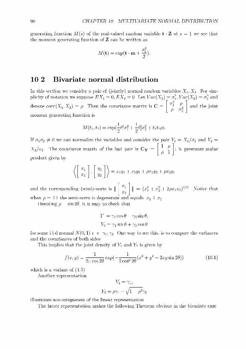
98 CHAPTER 10. MULTIVARIATE NORMAL DISTRIBUTION
generating function M(s) of the real-valued random variable t � Z at s = 1 we see thatthe moment generating function of Z can be written as
M(t) = exp(t �m+�2t2):
10.2 Bivariate normal distribution
In this section we consider a pair of (jointly) normal random variables X1; X2. For sim-plicity of notation we suppose EX1 = 0; EX2 = 0. Let V ar(X1) = �21 ; V ar(X2) = �22 and
denote corr(X1; X2) = �. Then the covariance matrix is C =
"�21 �� �22
#and the joint
moment generating function is
M(t1; t2) = exp(1
2t21�
21 +
1
2t22�
22 + t1t2�):
If �1�2 6= 0 we can normalize the variables and consider the pair Y1 = X1=�1 and Y2 =
X2=�2. The covariance matrix of the last pair is CY =
"1 �� 1
#; it generates scalar
product given by
*"x1x2
#;
"y1y2
#+= x1y1 + x2y2 + �x1y2 + �x2y1
and the corresponding (semi)-norm is jjj"x1x2
#jjj = (x21 + x22 + 2�x1x2)
1=2. Notice that
when � = �1 the semi-norm is degenerate and equals jx1 � x2j.Denoting � = sin 2�, it is easy to check that
Y1 = 1 cos � + 2 sin �;
Y2 = 1 sin � + 2 cos �
for some i.i.d normal N(0; 1) r. v. 1; 2. One way to see this, is to compare the variancesand the covariances of both sides.
This implies that the joint density of Y1 and Y2 is given by
f(x; y) =1
2� cos 2�exp(� 1
2 cos2 2�(x2 + y2 � 2xy sin 2�)) (10:1)
which is a variant of (4.5).Another representation
Y1 = 1;
Y2 = � 1 +q1� �2 2
illustrates non-uniqueness of the linear representation.The latter representation makes the following Theorem obvious in the bivariate case.

10.2. BIVARIATE NORMAL DISTRIBUTION 99
Theorem 10.2.1 Let X;Y be jointly normal.(i) If X;Y are uncorrelated, then they are independent.(ii) E(YjX) =m+ AX is linear(iii) Y � AX and X are independent.
Returning back to random variables X1; X2, we have X1 = 1�1 cos � + 2�1 sin � andX2 = 1�2 sin � + 2�2 cos �; this representation holds true also in the degenerate case.
10.2.1 Example: normal random walk
In this example we analyze a discrete time Gaussian random walk fXkg0�k�T . Let�1; �2; : : : be i. i. d. N(0; 1). We are interested in explicit formulas for the moment generat-ing function and for the density of the IRT -valued random variable X = (X1; X2; : : : ; XT ),where
Xk =kX
j=1
�j (10:2)
are partial sums.Clearly, m = 0. Equation (10.2) expresses X as a linear transformation X = Ag of
the i. i. d. standard normal vector with
A =
2666641 0 : : : 01 1 : : : 0...
. . ....
1 1 : : : 1
377775 :
Therefore from (10.5) we get
M(t) = exp1
2(t21 + (t1 + t2)
2 + : : :+ (t1 + t2 + : : :+ tT )2):
To �nd the formula for joint density, notice that A is the matrix representation of thelinear operator, which to a given sequence of numbers (x1; x2; : : : ; xT ) assigns the sequenceof its partial sums (x1; x1 + x2; : : : ; x1 + x2 + : : :+ xT ). Therefore, its inverse is the �nitedi�erence operator � : (x1; x2; : : : ; xT ) 7! (x1; x2 � x1; : : : ; xT � xT�1). This implies
A�1 =
26666666664
1 0 0 : : : : : : 0�1 1 0 : : : : : : 00 �1 1 : : : : : : 00 0 �1 : : : : : : 0...
. . .. . .
...0 : : : 0 : : : �1 1
37777777775:
Since detA = 1, we get
f(x) = (2�)�n=2 exp�1
2(x21 + (x2 � x1)
2 + : : :+ (xT � xT�1)2): (10:3)
Interpreting X as the discrete time process X1; X2; : : :, the probability density functionfor its trajectory x is given by f(x) = C exp(�1
2k�xk2).
Expression 12k�xk2 can be interpreted as proportional to the kinetic energy of the
motion described by the path x; assigning probabilities by Ce�Energy=(kT ) is a well knownpractice in statistical physics. In continuous time, the derivative plays analogous role.

100 CHAPTER 10. MULTIVARIATE NORMAL DISTRIBUTION
10.3 Simulating a multivariate normal distribution
To simulate any d-dimensional normal distribution we need only to simulate d independentN(0; 1) random variables and use linear representations like in Theorem 10.4.2. For suchsimulation the covariance matrix needs to be inverted and diagonalized, a numericalnuisance in itself. When the multivariate normal distribution occurs as the so-called timeseries, a method based on Fourier expansion is then convenient, see Section 11.4, or theintroductory examples in Chapter 12.
10.3.1 General multivariate normal law
The linear algebra results imply that the moment generating function corresponding to anormal distribution on IRd can be written in the form
M(t) = exp(t �m+1
2Ct � t): (10:4)
10.4 Covariance matrix
Theorem 3.2.2 identi�es m 2 IRd as the mean of the normal random variable Z =(Z1; : : : ; Zd); similarly, double di�erentiation M(t) at t = 0 shows that C = [ci;j] isgiven by ci;j = Cov(Zi; Zj). This establishes the following.
Theorem 10.4.1 The moment generating function corresponding to a normal randomvariable Z = (Z1; : : : ; Zd) is given by (10.4), where m = EZ and C = [ci;j], whereci;j = Cov(Zi; Zj), is the covariance matrix.
From (10.4) and linear algebra we get also
M(t) = exp(t �m+1
2(At) � (At)): (10:5)
We have the following multivariate generalization of (4.1).
Theorem 10.4.2 Each d-dimensional normal random variable Z has the same distribu-tion as m +Ag, where m 2 IRd is deterministic, A is a (symmetric) d � d matrix andg = ( 1; : : : ; d) is a random vector such that the components 1; : : : ; d are independentN(0; 1) random variables.
Proof. Clearly, Eexp(t � (m+Ag)) = exp(t �m)Eexp(t � (Ag)). Since the moment gen-erating function of g is Eexp(x � g) = exp 1
2kxk2 and t � (Ag) = (AT t) � g, therefore we
get Eexp(t � (m+Ag)) = exp t �m exp+12kATtk2, which is another form of (10.5). 2

10.4. COVARIANCE MATRIX 101
10.4.1 Multivariate normal density
Now we consider the multivariate normal density. The density of independent 1; : : : ; inTheorem 10.4.2 is the product of the one-dimensional standard normal densities, ie.
fg(x) = (2�)�d=2 exp(�1
2kxk2):
Suppose that detC 6= 0, which ensures that A is nonsingular. By the change of variableformula, from Theorem 10.4.2 we get the following expression for the multivariate normaldensity.
Theorem 10.4.3 If Z is centered normal with the nonsingular covariance matrix C, thenthe density of Z is given by
fZ(x) = (2�)�d=2(detA)�1 exp(�1
2kA�1xk2);
or
fZ(x) = (2�)�d=2(detC)�1=2 exp(�1
2C�1x � x);
where matrices A and C are related by C = A� AT .
In the nonsingular case the density expression implies strong integrability.
Theorem 10.4.4 If Z is normal, then there is � > 0 such that
Eexp(�kZk2) <1:
Remark 3 Theorem 10.4.4 holds true also in the singular case and for Gaussian random variables
with values in in�nite dimensional spaces.
10.4.2 Linear regression
For general multivariate normal random variablesX andY we have the following linearityof regression result.
Theorem 10.4.5 If (X;Y) has jointly normal distribution on IRd1+d2, then
EfXjYg = a +QY; (10:6)
Random vectors Y �QY and X are stochastically independent.
Vector a =mX�QmY and matrixQ are determined by the expected valuesmX;mY
and by the (joint) covariance matrix C (uniquely if the covariance CY of Y is non-singular). To �nd Q, multiply (10.6) (as a column vector) from the right by (Y � EY)T
and take the expected value. By Theorem A.2.1(i) we get Q = R�C�1Y , where we have
written C as the (suitable) block matrix C =
"CX RRT CY
#.
Problem 10.1 For the random walk from Section 10.2.1, what is E(XkjX1; : : : ; Xk�1; Xk+1; : : : ; Xn)?
Problem 10.2 Suppose X1; : : : ; Xd are jointly normal, EXj = 0; EX2j = 1 and all co-
variances EXiXj = � are the same for i 6= j.Find E(X1jX2; X3; : : : ; Xd). (Notice that in this example � > �1=d.)

102 CHAPTER 10. MULTIVARIATE NORMAL DISTRIBUTION
10.5 Gaussian Markov processes
Suppose (Xt)t=0;1;::: is a Markov chain with multivariate normal distribution. That is,suppose X0 is normal, and the transition probabilities are normal, too.
Without loss of generality we assume EXt = 0; EX2t = 1 and let EX0X1 = �. Then
E(Xt+1jXt) = �Xt and therefore EX0Xt = �t. This means that the covariance matrix ofthe Markov Gaussian process depends on one parameter � only. Comparing the answerwith Section 8.7 we �nd out that all homogeneous Markov Gaussian processes have theform Xt =
P1k=0 k+t�
k, where k are independent normal r. v.

Chapter 11
Continuous time processes
Continuous time processes are the families of random variables Xt, with t � 0 interpretedas time.
11.1 Poisson process
Poisson distribution occurs as an approximation to binomial. Another reason for itsoccurrence is related to exponential random variables and counting customers in queues.The latter is perhaps the most e�cient way of simulating Poisson random variables, seeSection 6.2.4. A related reason for the frequent use of Poisson distribution in modeling isthe law of rare events.
De�nition 11.1.1 A Poisson process of intensity � > 0 is an integer-valued stochasticprocess fNt :g with the following properties.
� N0 = 0
� For s > 0; t > 0 random variable Nt+s�Nt has Poisson distribution with parameter�s.
� Nt has independent increments
Suppose cars pass by an intersection and the times between their arrivals are independentand exponential. Thus we are given i. i. d sequence Tj of exponential r. v. (with parameter�). The number of cars that passed by within time interval (0; t) is a random variable Nt.Clearly, Nt is the �rst integer k such that T1 + : : : Tk > t.
Theorem 11.1.1 For t > 0; s > 0 random variable N(t+ s)�N(t) is independent of Nt
and has Poisson distribution Poiss(s�).
Proof. We will prove only that Nt has the Poisson distribution. To simplify notationassume that exponential r.`v. have parameter � = 1. We prove the formula Pr(Nt = k) =tk
k!e�t by induction.k = 0: Pr(Nt = 0) = Pr(T > t) =
R1t e�x dx = e�t
103

104 CHAPTER 11. CONTINUOUS TIME PROCESSES
Suppose the formula is true for k. Then
Pr(Nt = k + 1) = Pr(T1 + : : :+ Tk+1 > t) =Z 1
t1=�(k + 1)xke�x dx:
Integrating by parts we check that
Pr(Nt = k + 1) =t
k + 1Pr(Nt = k):
2
Similar processes are considered in reliability theory, and in queueing theory, also fornon-exponential sojourn times Tj.
Problem 11.1 Assume a device fails when a cumulative e�ect of k shocks occurs. Ifthe shocks occur according to the Poisson process with parameter �, what is the densityfunction for the life T of the device?
Problem 11.2 Let f(x; t) = Ef(x + Nt), where Nt is the Poisson process of intensity� = 1. Show that @f
@t= f(x+ 1)� f(x).
In particular, pt(k) = Pr(Nt = k) satis�es @pt(k)@t
= pt(k + 1)� pt(k).
Problem 11.3 Customers arrive at a facility at random according to a Poisson processof rate �. The customers are dispatched (processed) in groups at deterministic timesT; 2T; 3T; : : :.
There is a waiting time cost c per customer per unit of time, and a dispatch cost K.
� What is the mean total cost (customer waiting+dispatch cost) per unit of time duringthe �rst cycle?
� What value of T minimizes the mean cost per unit of time?
Problem 11.4 Find the mean ENt, variance V ar(Nt) and the covariance cov(Nt; Ns).
Problem 11.5 Let X(t) = (�1)Nt. Find the mean EXt, variance V ar(Xt) and thecovariance cov(Xt; Xs).
The rate � in the Poisson process has probabilistic interpretation:
� = limh!0
Pr(Nt+h �Nt = 1)
h(11:1)
In many applications we wish to consider rates �(t) that vary with time. The cor-responding process is just a time-change of the Poisson process X(t) = N�(t), where�(t) =
R t0 �(s)ds.

11.1. POISSON PROCESS 105
11.1.1 The law of rare events
Let N(I) denote the number of events that occur in interval I. We make the followingpostulates.
1. If intervals I1; : : : Ir are disjoint, then random variables fN(Ij)g are independent.2. For any t and h > 0 the probability distribution of N((t; t+ h]) does not depend on
t.
3. Pr(N(Ih)�2)h
! 0 as h! 0
4. Pr(N(Ih)=1)h
! � as h! 0
Theorem 11.1.2 Nt = N((0; t]) is the Poisson process of intensity �.
Example 11.1 A careless programmer assigns memory locations to the variables in hisprogram1 at random . Suppose that there are M ! 1 locations and N = �M variables.Let Xi be the number of variables assigned to each location. If each location is equallylikely to be chosen, show that
� Pr(Xi = k)! e���k=k! as N !1� Xi and Xj are independent in the limit for i 6= j.
In the limit, what fraction of memory locations has two or more variables assigned?
Example 11.2 While testing a program, the number of bugs discoverd in the programfollows the Poisson process with intensity � = 5 errors per hour. Tester's �ance entersthe test area and agrees to wait for the tester to �nd just one more bug. How long willshe wait on average: 12 minutes, or 6 minutes?
11.1.2 Compound Poisson process
The Poisson process Nt counts the number of events. If each event results in a random (andindependent) outcome �j, then the total is the compound Poisson process Z(t) =
PNtj=1 �j.
The moments and also the moment generating function of Z(t) can be determinedthrough conditioning. Section 7.5.1 implies that if E� = �, V ar(�) = �2 then E(Z(t)) =��t, V ar(Z(t)) = �(�2 + �2)t.
1Variable aliasing is the mistake of assigning the same location to two or more variables in a program.

106 CHAPTER 11. CONTINUOUS TIME PROCESSES
Examples
1. Risk assessment: Insurance company hasM customers. Suppose claims arrive at aninsurance company in accordance with the Poisson process with rate �M . Let Yk bethe magnitude of the k-th claim. The net pro�t of the company is then Z(t)�M�t,where � is the (�xed in this example) premium.
2. A shock model: Let Nt be the number of shocks to a system up to time t and let �kdenote the damage or wear incurred by the k-th shock.
If the damage accumulates additively, then Z(t) represents the total damage sus-tained up to time t. Suppose that the system continues to operate until this totaldamage is less than some critical value c and fails otherwise. Then the (random)failure time T satis�es T > t if and only if Z(t) < c. Therefore Pr(T > t) =P1
n=0 Pr(Pn
k=1 �k � zjNt = n)(�t)ne��t=n!. Thus ET = 1�
P1n=0 Pr(
Pnj=1 �j � c). In
particular if �k are exponential ET = 1+c��
.
11.2 Continuous time Markov processes
Given a discrete-time Markov chain, there are many ways of \running it" in continuoustime. One particular method is to make the moves at random moments of time. If theseinstances are exponential, then the resulting continuous-time process is Markov, too. Thisis the so-called embedded Markov chain.
Non-pathological continuous time Markov processes with countable state space haveembedded Markov chain representation. In such representation we run a continuous timeclock based on the independent exponential random variables. Once the time comes, weselect the next position according to the transition probabilities of a discrete-time Markovchain.
The theory of continuous time Markov chains (that is | processes with countablestate space) is similar to discrete time theory. The linear �rst-order di�erence equationsfor probabilities are replaced by the systems of �rst-order di�erential equations.
Example 11.3 Suppose Xn is a two-state Markov chain with the following transitions:0 7! 1 with probability a, 1 7! 0 with probability b. From Section 8.1 we know thatP (Xk = 1)! a=(a+ b) as k !1.
Let Tk be i. i. d. exponential r. v. and let Y (t) = Xk when T1 + : : : + Tk < t <T1 + : : :+ Tk+1.
Function p(t) = Pr(Y (t) = 1) satis�es di�erential equation: p0(t) = ��p(t) +�bp(t)+�a(1� p(t). Indeed, Pr(Y (t+ h) = 1) � Pr(Y (t) = 1; T > h) + Pr(Y (t) = 0; T < h).
Therefore p(t) = a=(a + b) + b=(a + b) exp(��(1� b+ a)t).
Here is a slightly di�erent method to run the continuous time �nite-valued Markovchain.
Pick the initial value according to prescribed distribution. Then select an exponentialrandom variable for each of the possible transitions. Each of these can have di�erentparameter �k. Then select the smallest, T = minTj. It can be shown that T is exponential
with parameterP�j and that Pr(T = Tj) =
�jPk�k.
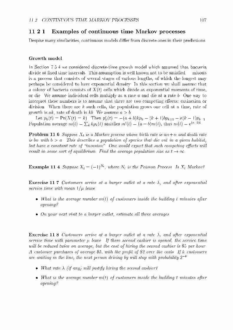
11.2. CONTINUOUS TIME MARKOV PROCESSES 107
11.2.1 Examples of continuous time Markov processes
Despite many similarities, continuous models di�er from discrete ones in their predictions.
Growth model
In Section 7.5.4 we considered discrete-time growth model which assumed that bacteriadivide at �xed time intervals. This assumption is well known not to be satis�ed | mitosisis a process that consists of several stages of various lengths, of which the longest mayperhaps be considered to have exponential density. In this section we shall assume thata colony of bacteria consists of X(t) cells which divide at exponential moments of time,or die. We assume individual cells multiply at a rate a and die at a rate b. One way tointerpret these numbers is to assume that there are two competing e�ects: extinction ordivision. When there are k such cells, the population grows one cell at a time, rate ofgrowth is ak, rate of death is kb. We assume a > b.
Let pk(t) = Pr(X(t) = k). Then p0k(t) = �(a + b)kpk + (k + 1)bpk+1 + a(k � 1)pk�1.Population average m(t) =
Pk kpk(t) satis�es m
0(t) = (a� b)m(t), thus m(t) = e(a�b)t.
Problem 11.6 Suppose Xt is a Markov process whose birth rate is an+� and death rateis bn with b > a. This describes a population of species that die out in a given habitat,but have a constant rate of \invasion". One would expect that such competing e�ects willresult in some sort of equilibrium. Find the average population size as t!1.
Example 11.4 Suppose Xt = (�1)Nt, where Nt is the Poisson Process. Is Xt Markov?
Exercise 11.7 Customers arrive at a burger outlet at a rate �, and after exponentialservice time with mean 1=� leave.
� What is the average number m(t) of customers inside the building t minutes afteropening?
� On your next visit to a burger outlet, estimate all three averages.
Exercise 11.8 Customers arrive at a burger outlet at a rate �, and after exponentialservice time with parameter � leave. If there second cashier is opened, the service timewill be reduced twice on average, but the cost of hiring the second cashier is $5 per hour.A customer purchases of average $5, with the pro�t of $2 over the costs. If k customersare waiting in the line, the next person driving by will stop with probability 2�k.
� What rate � (if any) will justify hiring the second cashier?
� What is the average number m(t) of customers inside the building t minutes afteropening?

108 CHAPTER 11. CONTINUOUS TIME PROCESSES
11.3 Gaussian processes
Continuous-time Markov processes with uncountable state space require more advancedmathematical tools. Only Gaussian case can be brie y mentioned here.
De�nition 11.3.1 A stochastic process fXtg0�t<1 is Gaussian, if the n-dimensional r. v.(Xt1 ; : : : ; Xtn) has multivariate normal distribution for all n � 1 and all t1; : : : ; tn 2[0;1).
11.4 The Wiener process
The simplest way to de�ne the Wiener process is to list its properties as follows.
De�nition 11.4.1 The Wiener process fWtg is a Gaussian process with continuous tra-jectories such that
W0 = 0; (11.2)
EWt = 0 for all t � 0; (11.3)
EWtWs = minft; sg for all t; s � 0: (11.4)
A stochastic process fXtgt2[0;1] has continuous trajectories if it is de�ned by a C[0; 1]-valued random vector, or if all of its paths are continuous2. For in�nite time intervalt 2 [0;1), a stochastic process has continuous trajectories if its restriction to t 2 [0; N ]has continuous trajectories for all N 2 IN.
Conditions (11.2){(11.4) imply that the Wiener process has independent increments,ie. W0;Wt �W0;Wt+s �Wt; : : : are independent.
Series expansions for the Wiener process are available in the literature. One way toobtain these is from Fourier expansion for the covariance function.
Problem 11.9 Let u(x; t) = Ef(Wt + x), where f is a smooth function. Show that usatis�es the parabolic equation @u
@t= 1
2@2u@x2
.
Problem 11.10 What partial di�erential equation is solved by u(x; t) = Ef(aWt+x+bt)when a; b are non-zero constants?
Scaled Wiener process is a good model of di�usion. Use the two-dimensional Wienerprocess to model a two-dimensional di�usion. The two-dimensional Wiener process isobtained from two independent one-dimensional components. The di�usion coe�cienta2 has units [length2/time] and is implemented by scaling the Wiener process: aWt hasdi�usion coe�cient a2.
Exercise 11.11 An eye-irritant pollutant is emitted from a factory chimney located atx = 0; y = 10 on the xy plane, and the wind blows left-to-right with velocity v(y) = yat height y. At a distance L = 100 down-wind, there is a residential building of height15. Which oor of the building is polluted the most? Is there a signi�cant di�erence inpollution level between the oors? (Assume that the distances are in units such that thedi�usion coe�cient is 1.)
2This is a very imprecise statement!

Chapter 12
Time Series
This chapter contains additional topics on discrete time processes. We begin with severalexamples of possible simulations. The resulting random curves are very di�erent, butthey have the same \mean-square" behavior.
Example 12.1 Suppose we wish to pick a curve at random. In other words, we need arandom function X(t) of integer parameter t. Here is one way to do it: take X(t) =P
k kak cos(kt), where k are i. i. d. normal N(0; 1). To ensure the series is convergentwe need
Pk a
2k <1; thus we can assume ak =
R 2�0 g(�) cos(k�) d�. The theory of Fourier
series tells us that ifRg2(�) <1, then the coe�cients ak are square-summable.
Example 12.2 Suppose we wish to pick a curve at random. Here is one way to do it:take X(t) =
Pcj cos(2�t + �j), where �j are independent and uniformly distributed on
the interval (0; 2�). Again select ck =R 2�0 g(�) cos(k�) d�.
Exercise 12.1 Write simulations of the curves as described. Pick as g a trigonometricpolynomial, say g(�) = 1 + cos(�) cos(2�).
12.1 Second order stationary processes
Stationary processes are those that their probabilistic characteristics (distributions, con-ditional distributions, moments, covariances) do not change with time.
Example 12.3 Suppose Xn is a Markov chain, and Pr(X0 = j) = �(j), where �j is itsinvariant distribution. Then (X0; Xk) �= (Xn; Xn+k).
For second-order stationary processes only means, variances, and covariances do notchange with time. That is, m(t) = EX(t) = const; cov(X(t); X(s)) = K(t � s). Thesecond-order theory of processes is a very coarse theory. Nevertheless, it does solve thebest linear prediction problem.
Proposition 12.1.1 In each of the introductory Examples, EX(t) = 0 andcov(X(t); X(s)) = K(t� s), where K(t) =
R 2�0 cos(�t)f(�) d�.
109

110 CHAPTER 12. TIME SERIES
12.1.1 Positive de�nite functions
The covariance K(t) of the weakly stationary process is a positive de�nite function. Thatis,
PcicjK(ti � tj) = EjPj cjX(tj)j2 � 0 for all cj 2 CC; tj 2 IR. In addition, K(t) =
K(�t).Theorem 12.1.2 Given a positive de�nite even function K : ZZ ! IR, there is a (0; 2�)-valued random variable � such that for all integer t
K(t) = K(0)E cos(t�): (12:1)
Proposition 12.1.3 Suppose � from Theorem 12.1.2 has density f(�). Let g(�) =qf(�)
and de�ne Xt as in Example 12.1. Then Xt is Gaussian, mean zero, with covariance(12.1).
12.2 Trajectory averages
When a time series Xt is observed,1n(X1 + : : : + Xn) is the \trajectory average". It is
interesting how does this compare to the \probabilistic" average EX.The following theorem follows immediately from the proof of Theorem 5.2.1. The
assumption holds true in particular when Xn has spectral density.
Theorem 12.2.1 Suppose Xn is weakly stationary. If cov(X0; Xn)! 0 as n!1 then1n(X1 + : : :+Xn)! EX in L2-norm.
Proof. Compute the variance, and use the Cesaro summability result (Theorem B.3.1). 2
The covariance argument can be rewritten in spectral notation. Suppose EX0Xk =(2�)�1
R ��� e
iksf(s) ds. Then E(X1 + : : : + Xn)2 = (2�)�1
R ��� j
Pnk=1 e
iksj2f(s) ds, so
V ar( 1n(X1 + : : :+Xn)) = (2�)�1 1
n2
R ���
sin2( 12ns)
sin2( 12s)f(s) ds! 0 as n!1.
12.3 The general prediction problem
The basic problem in �ltering and prediction is as follows. Given variables X1; : : : ; Xn,�nd the estimator of the value of Y with smallest quadratic error. Case n = 1 is presentedis Sections 2.11.1 and 2.14 for the linear and non-linear case.
In the linear prediction problem we deal with linear estimators a0 +P
j ajXj. Thequadratic error involves variances, covariances and averages only. Thus it is appropriateto handle this in through the second order processes, and the solution should depend onthe density of � - the so called spectral density only.
The general Hilbert space theory tells us that the best linear prediction of Xt+1 basedon the past is
Ptj=0 ajXj with coe�cients aj such that EXj(Xt+1�Pt
j=0 ajXj) = 0 for all0leqj � t. This is a system of t+1 linear equations for t+1 unknown coe�cients. Gramm-Schmidt orthogonalization allows to replace Xj by orthonormal �j. Optimal predictionuses
Ptj=0 �j�j with �j = EX0�t�j.

12.4. AUTOREGRESSIVE PROCESSES 111
12.4 Autoregressive processes
Suppose �k are i. i. d. A stochastic process Xt is an autoregressive process, if it satis�esa linear di�erence equation
Xt+1 =dX
j=0
ajXt�j + �t+1 (12:2)
with random coe�cients �t+1.
Example 12.4 Autoregressive process Xt+1 = aXt + �t+1 is Markov. For jaj < 1 it hasa stationary distribution. What is it? What happens for jaj > 1?
Example 12.5 A moving average Xt+1 =1d
Pdj=1 �t�j is an autoregressive process. What
is the corresponding di�erence equation (12.2)?
For autoregressive process the optimal one-step prediction of Xt+1 is
dXj=0
aja0Xt�j: (12:3)
The spectral theory asserts that this is best linear prediction. However if �j are i. i. d.,then this is actually optimal non-linear prediction as well.
More general autoregressive sequences are de�ned as solutions of
dXj=0
ajXt�j =Xi
bi�t�i (12:4)
These generalize simultaneously autoregressive and moving average processes.

112 CHAPTER 12. TIME SERIES

Chapter 13
Additional topics
13.1 A simple probabilistic modeling in Genetics
First we describe the population at a single instance. We consider the model in whicheach hereditary character is carried by a pair of genes. For simplicity, we assume only one(pair) of a gene, and only one hereditary character corresponding to one locus. There areseveral possible alleles (categories) in a locus { we assume there are only two, denotedby a; A, of which A is dominant. Each individual thus is described by one of the pairsAA;Aa; aa, the so called phenotype . However, a is obstructed from the view by A, thusfor an outside observer individuals AA and Aa are indistinguishable. A statistical studyof such a population can only yield the proportion PA of individuals with "A-feature",and not the actual probabilities of the three possible phenotype.
Now we turn to the modelling of the generation change. Under simple assumptions weshall be able to �nd out what are the frequencies of phenotype and genotypes. Usuallythis information is not directly available. We assume that the next generation occurs byrandom mating. Let pAA(0); pAa(0); paa(0) be the actual (and as yet unknown) probabili-ties of the phenotype. Under random mating with independent selection of parents, theprobability that an o�spring has phenotype AA is pAA(1) = (pAA(0) +
12pAa(0))
2.Denoting by pA(t) = pAA(t) +
12pAa(t) we get the Hardy-Weinberg equilibrium: after
one generation the proportions pA(t) of genotypes stabilize and the phenotype frequenciesbecome
PAA = p2A (13.1)
PAa = 2papA (13.2)
Paa = p2a (13.3)
(13.4)
This determines the actual proportions of the phenotype from the proportion of ob-served A-carriers and a-carriers.
Problem 13.1 Show that PAa = 2(pPaa � Paa).
The next question is to study the e�ects of the selection, where, say phenotype aa hasdi�erent chance of survival. This leads to total probability formula and Markov chains.
113

114 CHAPTER 13. ADDITIONAL TOPICS
13.2 Application: verifying matrix multiplication
Suppose one has an algorithm to multiply large matrices and we want to check if the outputis correct. A possible method is to pick the vector X of 0; 1 and check if ABX = CX.This is the so called Freivalds technique
Theorem 13.2.1 If A;B;C are n � n matrices such that AB 6= C then Pr(ABX =CX) � 1
2.
Proof. For a non-zero v we have Pr(jv �Xj > 0) < 122
13.3 Exchangeability
De�nition 13.3.1 A sequence (Xk) of random variables is exchangeable, if the joint dis-tribution of X�(1); X�(2); : : : ; X�(n) is the same as the joint distribution of X1; X2; : : : ; Xn
for all n � 1 and for all permutations � of f1; 2; : : : ; ng.
The following beautiful theorem due to B. de Finetti points out the role of exchange-ability as a substitute for independence.
Theorem 13.3.1 Suppose that X1; X2; : : : is an in�nite exchangeable sequence. Thenthere exist a �-�eld N such that X1; X2; : : : are N -conditionally i. i. d., that is
P (X1 < a1; X2 < a2; : : : ; Xn < anjN )
= P (X1 < a1jN )P (X1 < a2jN ) : : : P (X1 < anjN )
for all a1; : : : ; an 2 IR and all n � 1.
We will use the following (weak) version of the martingale1 convergence theorem.
Theorem 13.3.2 Suppose Fn is a decreasing family of �-�elds, ie. Fn+1 � Fn for alln � 1. If X is integrable, then EfXjFng ! EfXjFg in L1-norm, where F is theintersection of all Fn.
Proof. Suppose �rst that X is square integrable. Subtracting m = EX if necessary,we can reduce the convergence question to the centered case EX = 0. Denote Xn =EfXjFng. Since Fn+1 � Fn, by Jensen's inequality EX
2n � 0 is a decreasing non-negative
sequence. In particular, EX2n converges.
Let m < n be �xed. Then E(Xn �Xm)2 = EX2
n+EX2m� 2EXnXm. Since Fn � Fm,
by Theorem A.2.1 we have
EXnXm = EEfXnXmjFng = EXnEfXmjFng1A martingale with respect to a family of increasing �-�elds Fn is and integrable sequence Xn such
that E(Xn+1jFn) = Xn. The sequence Xn = E(X jFn) is a martingale. The sequence in the theorem isof the same form, except that the �-�elds are decreasing rather than increasing.

13.3. EXCHANGEABILITY 115
= EXnEfEfXjFmgjFng = EXnEfXjFng = EX2n:
Therefore E(Xn �Xm)2 = EX2
m � EX2n. Since EX
2n converges, Xn satis�es the Cauchy
condition for convergence in L2 norm. This shows that for square integrable X, sequencefXng converges in L2.
If X is not square integrable, then for every � > 0 there is a square integrable Y suchthat EjX � Y j < �. By Jensen's inequality EfXjFng and EfY jFng di�er by at most �in L1-norm; this holds uniformly in n. Since by the �rst part of the proof EfY jFng isconvergent, it satis�es the Cauchy condition in L2 and hence in L1. Therefore for each� > 0 we can �nd N such that for all n;m > N we have EfjEfXjFng�EfXjFmgjg < 3�.This shows that EfXjFng satis�es the Cauchy condition and hence converges in L1.
The fact that the limit is X1 = EfXjFg can be seen as follows. Clearly X1 isFn-measurable for all n, ie. it is F -measurable. For A 2 F (hence also in Fn), wehave EXIA = EXnIA. Since jEXnIA � EX1IAj � EjXn �X1jIA � EjXn �X1j ! 0,therefore EXnIA ! EX1IA. This shows that EXIA = EX1IA and by de�nition,X1 = EfXjFg. 2
Proof of Theorem 13.3.1. Let N be the tail �-�eld, ie.
N =1\k=1
�(Xk; Xk+1; : : :)
and put Nk = �(Xk; Xk+1; : : :). Fix bounded measurable functions f; g; h and denote
Fn = f(X1; : : : ; Xn);
Gn;m = g(Xn+1; : : : ; Xm+n);
Hn;m;N = h(Xm+n+N+1; Xm+n+N+2; : : :);
where n;m;N � 1. Exchangeability implies that
EFnGn;mHn;m;N = EFnGn+r;mHn;m;N
for all r � N . Since Hn;m;N is an arbitrary bounded Nm+n+N+1-measurable function, thisimplies
EfFnGn;mjNm+n+N+1g = EfFnGn+r;mjNm+n+N+1g:Passing to the limit as N !1, see Theorem 13.3.2, this gives
EfFnGn;mjNg = EfFnGn+r;mjNg:Therefore
EfFnGn;mjNg = EfGn+r;mEfFnjNn+r+1gjNg:Since EfFnjNn+r+1g converges in L1 to EfFnjNg as r !1, and since g is bounded,
EfGn+r;mEfFnjNn+r+1gjNgis arbitrarily close (in the L1 norm) to
EfGn+r;mEfFnjNgjNg = EfFnjNgEfGn+r;mjNg

116 CHAPTER 13. ADDITIONAL TOPICS
as r !1. By exchangeability EfGn+r;mjNg = EfGn;mjNg almost surely, which provesthat
EfFnGn;mjNg = EfFnjNgEfGn;mjNg:Since f; g are arbitrary, this proves N -conditional independence of the sequence. Us-ing the exchangeability of the sequence once again, one can see that random variablesX1; X2; : : : have the same N -conditional distribution and thus the theorem is proved. 2
13.4 Distances between strings
A string is a sequence of letters, or symbols from the �nite alphabet. For the purposeof computer modelling, we can assume that a string is a sequence of natural numbersf1; : : : dg, parameter d being the size of the alphabet.
Three simple examples of strings are the words, sentences in, say, English, and DNAmolecules. Here d = 26 (for lower-case words), d = 94 for sentences, and d = 6 for theDNA (there are only four proteins, but extra symbols are used to mark various undecidedcases).
The question of comparing two strings for similarities arises in molecular biology andin designing a spell-checker, or a speech recognition system. Accordingly, one would like tosay which strings are similar, and how likely it is that they are similar due to chance only.Additional complications arise from the fact that two strings compared do not necessarilyhave the same length.
A simple way to compare two strings is to measure the number of symbols that don'tmatch (the hamming distance). For instance abbacd and babacd would then have distance2. But abbacd and bbacda would have distance 6, even though they di�er just by onetransposition.
A less obvious way to compare two strings is to measure the edit distance: how manyediting operations are needed to transform one of the strings into another. Usually theediting operations are:
� insert a symbol
� delete a symbol
� replace a symbol
� transpose two consecutive symbols
These are suitable for spell-checkers, where it is known that about 80% of typing errorsare of the above form, thus most of mistyped words have edit-distance 1 from the original.
Accordingly, the edit distance is set to 0, if the words are identical, 1 if they di�er bya single error of one of the listed types, 2 if there were two such errors, etc. Formally, it isde�ned as the smallest number of elementary \TE" transformations required to transformone of the words into another.
The method of computation is based on recurrence. It is easy to see that a number oftransformations between and empty word and another one is exactly the length2 of the
2Only deletions are required.

13.4. DISTANCES BETWEEN STRINGS 117
word. If the two words U;W are formed from shorter ones U0;W0 by adding letters atthe end, then the distance Dist(U;W ) is the smallest of the numbers
� Dist(U0;W ) + 1 (delete)
� Dist(U;W0) + 1 (add)
� Dist(U0;W0) + 0 or 1 if same letter is added di�erent letter (swap)
� Dist(U00; V 00) + 1, if the last two letters are identical (transpose), where U00; V 00
are U0;W0 with last letter removed.
Here is a complete VB-listing:
Function Dist (U$, V$) As Integer
'Returns the edit distance
'(number of elementary changes: replacement, deletion, insertion,transposition)
'that are required to transform word U$ into V$
'
'Declare auxiliary variables
Dim m As Integer, n As Integer, j As Integer, i As Integer
Dim x As Integer, y As Integer, z As Integer, A$, B$
If Len(U$) < Len(V$) Then A$ = U$: B$ = V$: Else A$ = V$: B$ = U$
m = Len(A$)
n = Len(B$)
'Declare matrix of distances between substrings of i,j characters
ReDim D(m, n) As Integer
'Assign boundary values: distances from empty string
For i = 0 To m: D(i, 0) = i: Next i
For j = 1 To n: D(0, j) = j: Next j
'
'Main recurrence: Compute next distance D(i,j) from previously found values
For i = 1 To m
For j = 1 To n
x = D(i - 1, j) + 1 'delete character
y = D(i, j - 1) + 1 'inserte character
x = Intmin(x, y) 'choose better (Integer Minimum)
y = D(i - 1, j - 1) - (Mid$(A$, i, 1) <> Mid$(B$, j, 1)) 'swap characters i
x = Intmin(x, y) ' choose better
z = 0
If i > 1 And j > 1 Then
'If Mid$(A$, i, 1) <> Mid$(B$, j, 1) Then
z = (Mid$(A$, i, 1) = Mid$(B$, j - 1, 1)) * (Mid$(A$, i - 1, 1) = Mid$(
'End If
y = (1 + D(i - 2, j - 2)) * z + x * (1 - z)
x = Intmin(x, y)
End If
D(i, j) = x

118 CHAPTER 13. ADDITIONAL TOPICS
Next j
Next i
Dist = D(m, n)'current value
End Function
The main problem with edit distance to analyze DNA molecules is processing time.
Exercise 13.2 Write a program computing the edit distance between strings, and anotherone, which does the editing by simulation. (Try the randomization based on randomnumber of edit operations from the currently best candidate)
13.5 A model of cell growth
A cell in its growth goes through several phases, which have di�erent probabilistic char-acteristics. In a simple model, the cell doubles after a random time, which is the sum ofthe exponential and deterministic portion. The average of the exponential phase can beassumed to depend on the external circumstances.
Questions of interest
How does the growth of cells a�ect other cells? How to control mixed populations of cellsto stay within prescribed limits?
13.6 Shannon's Entropy
Let X1; : : :Xn be independent identically distributed (i. i. d.) discrete r. v with k values,say fv1; : : : ; vkg. Put X = (X1; : : : ; Xk).
For a �xed vector y we have thus the joint probability mass function f(x) = Pr(X =x). The average information H(X) contained in X is de�ned as
H(X) = �E log f(X) = �Xx
f(x) log f(x) (13:5)
Problem 13.3 Prove Gibbs' inequalityP
j pj log pj �Ppj log qj for all qj > 0;
Pqj = 1.
Notice that H(X) � 0 and H(X) � log k
13.6.1 Optimal search
Coding
Hu�man's code
Problem 13.4 Suppose you have 15 identical in appearance coins, except that one ofthem has a di�erent weight. Find the optimal3 weighting strategy to identify the odd coinby using a scale.
3That is, �nd the strategy that costs the least if you have to pay for each use of the scale.
13.7. APPLICATION: SPREAD OF EPIDEMIC 119
13.7 Application: spread of epidemic
Modeling of the spread of disease is complicated due to multiple factors that in uenceits development. The birth-and-death process does not seem to be a good model forthe spread of an epidemic in a �nite population, since when a large proportion of thepopulation has been infected, we cannot suppose that the rate of infections is independentof past history.

120 CHAPTER 13. ADDITIONAL TOPICS

Appendix A
Theoretical complements
A.1 Lp-spaces
Inequalities related to expected values are best stated in geometric language of norms andnormed spaces. We say that X 2 Lp, if X is p-integrable, i.e. EjXjp <1. In particular,X is square integrable if EX2 <1.
The Lp norm is
kXkp =(
p
qEjXjp if p � 1;
ess supjXj if p =1:
Notice that kX � EXk2 is just the standard deviation.We say that Xn converges to X in Lp, if kXn �Xkp ! 0 as n!1. If Xn converges
to X in L2, we shall also use the phrase sequence Xn converges to X in mean-square. Anexample of the latter is Theorem 5.2.1.
Several useful inequalities are collected in the following.
Theorem A.1.1 (i) for 1 � p � q � 1 we have Minkowski's inequality
kXkp � kXkq: (A:1)
(ii) for 1=p+ 1=q = 1, p � 1 we have H�older's inequality
EXY � kXkpkY kq: (A:2)
(iii) for 1 � p � 1 we have triangle inequality
kX + Y kp � kXkp + kY kp: (A:3)
Special case p = q = 2 of H�older's inequality (A.2) reads EXY � pEX2EY 2. It is
frequently used and is known as the Cauchy-Schwarz inequality.For the proof of Theorem A.1.1 we need the following elementary inequality.
Lemma A.1.2 For a; b > 0; 1 < p <1 and 1=p+ 1=q = 1 we have
ab � ap=p+ bq=q: (A:4)
121

122 APPENDIX A. THEORETICAL COMPLEMENTS
Proof. Function t 7! tp=p + t�q=q has the derivative tp�1 � t�q�1. The derivative ispositive for t > 1 and negative for 0 < t < 1. Hence the maximum value of the functionfor t > 0 is attained at t = 1, giving
tp=p+ t�q=q � 1:
Substituting t = a1=qb�1=p we get (A.4). 2
Proof of Theorem A.1.1 (ii). If either kXkp = 0 or kY kq = 0, then XY = 0a. s. Therefore we consider only the case kXkpkY kq > 0 and after rescaling we assumekXkp = kY kq = 1. Furthermore, the case p = 1; q = 1 is trivial as jXY j � jXjkY k1.For 1 < p <1 by (A.4) we have
jXY j � jXjp=p+ jY jq=q:Integrating this inequality we get jEXY j � EjXY j � 1 = kXkpkY kq. 2
Proof of Theorem A.1.1 (i). For p = 1 this is just Jensen's inequality; for a moregeneral version see Theorem A.2.1. For 1 < p <1 by H�older's inequality applied to theproduct of 1 and jXjp we have
kXkpp = EfjXjp � 1g � (EjXjq)p=q(E1r)1=r = kXkpq;where r is computed from the equation 1=r + p=q = 1. (This proof works also for p = 1with obvious changes in the write-up.) 2
Proof of Theorem A.1.1 (iii). The inequality is trivial if p = 1 or if kX + Y kp = 0.In the remaining cases
kX + Y kpp � Ef(jXj+ jY j)jX + Y jp�1g = EfjXjjX + Y jp�1g+ EfjY jjX + Y jp�1g:By H�older's inequality
kX + Y kpp � kXkpkX + Y kp=qp + kY kpkX + Y kp=qp :
Since p=q = p� 1, dividing both sides by kX + Y kp=qp we get the conclusion. 2
A.2 Properties of conditional expectations
In more advanced courses conditional expectation E(XjY ) is de�ned as a random variable�(Y ) that satis�es EXf(Y ) = E�(Y )f(Y ) for all bounded measurable (or just continu-ous) functions f .
The next theorem lists useful properties of conditional expectations.
Theorem A.2.1 (i) If Y = f(Z) is such that X and XY are integrable, thenEfXY jZg = Y EfXjZg;

A.2. PROPERTIES OF CONDITIONAL EXPECTATIONS 123
(ii) EXEX;Y = EX;
(iii) If (X; Y ) and Z are independent, then EfXjY; Zg = EfXjY g;(iv) If g(x) is a convex function and Ejg(X)j <1, then g(EfXjY g) � Efg(X)jY g;(v) If Y is non-random, then EfXjY g = EX;
(vi) If X; Y are integrable and a; b 2 IR then EfaX + bY jZg = aEfXjZg+ bEfY jZg;(vii) If X and Y are independent, then EfXjY g = EX.
Remark 4 Inequality (iv) is known as Jensen's inequality and this is how we shall refer to it.
The abstract proof uses the following1.
Lemma A.2.2 If Y1 and Y2 are F-measurable andRA Y1 dP � R
A Y2 dP for all A 2 F ,then Y1 � Y2 almost surely. If
RA Y1 dP =
RA Y2 dP for all A 2 F , then Y1 = Y2.
Proof. Let A� = fY1 > Y2 + �g 2 F . SinceRA� Y1 dP � R
A� Y2 dP + �P (A�), thusP (A�) > 0 is impossible. Event fY1 > Y2g is the countable union of the events A� (with� rational); thus it has probability 0 and Y1 � Y2 with probability one.
The second part follows from the �rst by symmetry. 2
Proof of Theorem A.2.1.(i) This is veri�ed �rst for Y = IB (the indicator function of an event B 2 F).
Let Y1 = EfXY jFg; Y2 = Y EfXjFg. From the de�nition one can easily see that bothRA Y1 dP and
RA Y2 dP are equal to
RA\BX dP . Therefore Y1 = Y2 by the Lemma A.2.2.
For the general case, approximate Y by simple random variables and use (vi).(ii) This follows from Lemma A.2.2: random variables Y1 = EfXjFg, Y2 = EfXjGg
are G-measurable and for A in G bothRA Y1 dP and
RA Y2 dP are equal to
RAX dP .
(iii) Let Y1 = EfXjN WFg; Y2 = EfXjFg. We check �rst thatZAY1 dP =
ZAY2 dP
for all A = B \ C, where B 2 N and C 2 F . This holds true, as both sides of theequation are equal to P (B)
RC X dP . Once equality
RA Y1 dP =
RA Y2 dP is established for
the generators of the �-�eld, it holds true for the whole �-�eld N WF ; this is standardmeasure theory2.
(iv) Here we need the �rst part of Lemma A.2.2. We also need to know that eachconvex function g(x) can be written as the supremum of a family of a�ne functionsfa;b(x) = ax + b. Let Y1 = Efg(X)jFg; Y2 = fa;b(EfXjFg); A 2 F . By (vi) we haveZ
AY1 dP =
ZAg(X) dP � fa;b(
ZAX) dP = fa;b(
ZAEfXjFg) dP =
ZAY2 dP:
Hence fa;b(EfXjFg) � Efg(X)jFg; taking the supremum (over suitable a; b) ends theproof.
(v), (vi), (vii) These proofs are left as exercises. 2
1Readers not familiar with measure theory should skip the proofs.2See � � � Theorem (Theorem 3.3) P. Billingsley, Probability and measure, Wiley, New York 1986.

124 APPENDIX A. THEORETICAL COMPLEMENTS
Problem A.1 Prove part (v) of Theorem A.2.1.
Problem A.2 Prove part (vi) of Theorem A.2.1.
Problem A.3 Prove part (vii) of Theorem A.2.1.
Problem A.4 Prove the following conditional version of Chebyshev's inequality: ifEjXj <1, then
P (jXj > tjY ) � EfjXj jY g=talmost surely.
Problem A.5 Show that if (U; V;X) are such that in distribution (U;X) �= (V;X) thenEfU jXg = EfV jXg almost surely.
Problem A.6 Show that if X; Y are integrable non-degenerate random variables, suchthat
EfXjY g = aY; EfY jXg = bX;
then jabj � 1.
Problem A.7 Show that if X; Y are integrable such that EfXjY g = Y and EfY jXg =X, then X = Y a. s.

Appendix B
Math background
The following sections are short reference on material from general math (calculus, linear algebra, etc).
B.1 Interactive links
The following links are operational as of March 21, 1996. Please note that these may change at any time.
� real analysis1 is available online.
B.2 Elementary combinatorics
The art of counting is called combinatorics. Here is a short listing of the formulas. All are the consequencesof the product rule of counting.
Permutations:Permutation is an arrangement (ordering) of k out of n distinct objects without repetitions. Thenumber of permutations is n!
(n�k)! . In particular, the number of ways to order n objects is n!
Combinations: Combinations are k-element subsets of n distinct elements. The number of combinationsis (nk ).
Variations: Variations are arrangements of k out of n distinct objects with repetitions allowed. Thenumber of variations is nk
B.3 Limits
The following limit can be computed by L'Hospital rule.
limn!1
(1 + a=n)n = ea (B:1)
The Cesaro summability formula is
Theorem B.3.1 If an ! a then 1n (a1 + : : :+ an)! a.
1http://www.shu.edu/projects/reals/reals.html
125

126 APPENDIX B. MATH BACKGROUND
B.4 Power series expansions
The following power series expansions are of interest in this course.
ex =
1Xk=0
xk=k! (B.2)
1
1� x=
1Xk=0
xk (B.3)
They give immediately the expansions
ln 1 + x =1Xk=0
(�1)k xk+1
k + 1(B.4)
ex2=2 =
1Xk=0
(B.5)
Z x
0
e�t2=2 dt =
1Xk=0
(B.6)
(B.7)
In particular for x > 0 we have ln 1 + x < x and ln 1 + x > x� x2=2.
B.5 Multivariate integration
Suppose x = x(u; v); y = y(u; v). The change of variables formula in multivariate case isZ ZU
f(x; y) dxdy =
Z ZV
f(x(u; v); y(u; v))jJ(u; v)j dudv; (B:8)
where the Jacobian J is given by
J = det
�@x@u
@x@v
@y@u
@y@v
�(B:9)
B.6 Di�erential equations
The solution of the linear di�erential equation y0 + ay = g(x) with y(0) = y0 is given by y(x) =y0e
�ax R x0 eatg(t)=; dt.
Second order linear equation y00+ay0+by = g(x) is often solved by the method of varying a constant.The �rst step is to solve the homogenous equation y00 + ay0 + by = 0 �rst using y = erx. The generalsolution of homogenous equation is y = C1e
r1x + C2er2x, or y = C1e
rx + C2xerx if the characteristic
equation has double root.
B.7 Linear algebra
De�nition B.7.1 A scalar product of vectors in V is a bilinear, positive de�nite, non-degenerate mappingh�j�i : V � V! IR.
De�nition B.7.2 Vectors x;y are orthogonal with respect to scalar product hji, if hxjyi = 0.
The length of a vector is kxk =phxjxi. Orthogonal vectors of unit length are called orthonormal..
If ej are the orthonormal vectors and x is in their linear span, then the coe�cients in the expansionx =
Pj ajej are given by aj = hxjeji.
Example B.1 Let V be the vector space of all continuous functions on the interval [��; �]. In the scalarproduct hf jgi = R ��� f(t)g(t) dt the functions fsin kgk2IN; fcosktgk2IN; 1 are orthogonal.

B.8. FOURIER SERIES 127
B.8 Fourier series
The Fourier series for a function f(x) is the expansion f(x) =P
n an sin�nx+bn cos�nx. Every periodiccontinuous function f can be expanded in the Fourier series. The coe�cients are
b0 =1
�
Z �
��f(x) dx (B.10)
bn =1
2�
Z �
��f(x) cosn�x dx for n 6= 0 (B.11)
an =1
2�
Z �
��f(x) sinn�x dx (B.12)
(B.13)
Example B.2 Expand jxj into the Fourier series, and graph the corresponding partial sums.
B.9 Powers of matrices
The Cayley - Hamilton theorem asserts that each d � d matrix A satis�es the polynomial equationQd(A) = 0, where Qd(x) = det(A� xI) is the characteristic polynomial of degree d.
This implies that An = a0(n)I + a1(n)A + : : : + ad�1(n)Ad�1, where xn = D(x)Q(x) + a0(n) +a1(n)x + : : : + ad�1(n)xd�1. If A has n distinct eigenvalues �j , the coe�cients aj(n) can be found bysolving the system of equations �nj = a0(n) + a1(n)�j + : : :+ ad�1(n)�
d�1j .
A quick method that �nds a characteristic polynomial due to K... is to solve the system of linearequations for the coe�cients: pick a vector X at random and solve2 for a0; : : : ; ad�1 the equationsa0X+a1AX+ : : :+ad�1Ad�1X = 0. If the resulting matrix is singular, re-sample X until a non-singularmatrix is found.
2Use Gaussian elimination.

128 APPENDIX B. MATH BACKGROUND

Appendix C
Numerical Methods
Calculators and more sophisticated math-geared software have e�cient numerical methods built-in. Hereare short prescriptions that may be used by general programmer. A more complete source is e.g.NumericalRecipes: The Art of Scienti�c Computing series.
C.1 Numerical integration
To approximate the integralR ba f(x) dx in calculus we use left and right sums: Ln = b�a
n
Pn�1k=0 f(a+
b�an k),
Rn = b�an
Pnk=1 f(a+
b�an k)
The more exact trapezoidal rule usesR baf(x) dx � Sn = 1
2 (Ln +Rn).
Still more powerful and easy to program integration method is the Simpson rule:R ba f(x) dx �
43S2n � 1
3Sn. The Simpson rule is exact for cubic polynomials. Typical way to program it is to call thesubroutine performing trapezoid method integration twice. Many calculators have Simpson rule build in.Before you use it, be sure to check if it is reliable enough. A simple test that catches some poorly written
routines isR 5000
e�x2
dx �p�=2.
C.2 Solving equations
The fast and powerful bisection method requires correct end-points, and �nds one solution only. But ithas virtually no assumptions, except the continuity: If f(x) is continuous and f(a) < 0; f(b) > 0 thenthere is a < x < b such that f(x) = 0 and the interval length can be halved by computing f(a+b2 ).
Three di�culties arise in real applications.
� How to �nd a \correct" initial pair
� How to �nd more than one solution
� How to solve systems of equations in several unknowns
The second point has satisfactory answer for polynomial equations. The third point can be tackledthrough search for minimum. Namely, if equations are f(x; y) = 0; g(x; y) = 0 then we need to �ndminima of f2(x; y) + g2(x; y).
C.3 Searching for minimum
The analog of the bisection method for �nding minima is to begin with three points a < b < c suchthat f(b) is the smallest of the three. The next triple is produced by partitioning the larger of the two
129

130 APPENDIX C. NUMERICAL METHODS
segments in proportion1 3�p5
2 � 0:38197, and comparing the resulting four values to pick the narrowertriplet.
1This is golden section. The explanation why it occurs here can be found in numerical methods books.

Appendix D
Programming Help
Programming help is grouped by the type of software. Currently available (as of March 21, 1996) arepreliminary versions of:
� Help for TI85 Programmable calculator1
D.1 Introducing BASIC
Any DOS-running PC comes also with BASIC. You can start it with the commandQBASIC
from the DOS command line, or from Windows File Manager (click on an entry QBASIC.EXE, usuallylocated in). If you are a devoted Windows user, you may install an Icon in Program Manager to runBASIC with a click of the mouse.
Correctly written programs halt at the end. But not all programs do that, so an \emergency exit" isbuild in.
To stop the execution of any program, press simultaneously Ctrl + Break .
how to use this chapter
This text was written for a complete novice to BASIC. If you �t the description, read the pages below,and type in each of the sample programs. Once you have them in the QBASIC, run them to see thee�ects of various instrunctions.
There is no possibility that by running these programs you will do any harm to your equipment.Experiment, and if something goes realy wrong, you can always turn OFF or restart the computer.
D.2 Computing
The mathematical conventions in QBASIC are 2^(1/2) for 21=2 , SQR(13) forp13, LOG(2) for the
natural logarithm ln 2, etc. With these, one can use QBASIC as a calculator. For instance the instructionPRINT LOG(1+2^(1/2))
will print the decimal value of the expression ln(1+p2). This probably is the simplest program to begin
with. It is so short that there is no point in saving it.The real power comes from repetitive operations explained in Section D.4.
1http://math.uc.edu/~brycw/preprint/ti85
131

132 APPENDIX D. PROGRAMMING HELP
D.3 The structure of a program
BASIC programs are actually text �les. The instructions are read consecutively by the BASIC interpreter.The QBASIC interpreter that comes with DOS is su�cient for our purposes. Sample programs belowintroduce certain more exotic build-in functions.
Example D.1 The following simple program prints current date & time
PRINT "HELLO"
PRINT "Today is "; DATE$
PRINT TIME$
Besides the actual code, programs should contain comments with explanations of instructions andtheir purpose. Comments and explanations in the program can be hidden from the processor through REM
command. Everything in a line after this command is skipped (the only exception being metacommands,which we don't have to concern ourselves with here). The sample2 programs, use a shortcut ' instead ofthe full command REM. This is faster to type and equivalent in action.
Example D.2 Here is the previous program with comments
'Prints current date & time
PRINT "HELLO" 'greet the user
PRINT "Today is "; DATE$ 'print date
PRINT TIME$ ' print time could have printer TIMER=# seconds since 1980
The typical program consists of the main module with fairly general instructions that call subroutinesto perform speci�c jobs, and a number of subprograms that are marked in text by SUB ... END SUB,and are displayed separately by the QBASIC Editor. Subprograms make it easier to write, test, andmaintain the program.
Within QBasic the SUBs are separated, each in each own text window, but the �nal program is savedas one �le with SUBs following the main module. To create a SUB, choose New SUB from the Editmenu. More details follow in Section D.9.
Larger projects often use several modules3 that are compiled and run together.
Example D.3 Here is the revision of the previous program with a simple but useful SUB.
'Prints current date & time in the middle of the screen
CLS 'clear display
CenterPrint "HELLO" 'greet the user
CenterPrint "Today is " & DATE$ 'print date - string has to be concatenated
CenterPrint TIME$ ' print time could have printer TIMER=# seconds since 1980
SUB CenterPrint (Text$)
'**** print text Text$ centered on screen
l=41-LEN(Text$)/2
if l<0 then l=0 'too long text cannot be centered
print TAB(l); Text$
New things: CLS, concatenation of strings, calling SUB, screen positioning by TAB, LEN("hello")
Every subprogram should begin with a (commented) short description of its purpose, and the meaningof parameters.
2The actual sample programs on the disk also contain commented LaTEX typesetting instructions atthe beginning and at the end. Their sole purpose is to insert the listings into this text.
3For example, in many applied math programs there is a need for integration routines. These perhapswould be collected in a separate module to facilitate repeated usage.

D.4. CONDITIONALS AND LOOPS 133
D.4 Conditionals and loops
Loops of �xed size are best handled byFOR j=1 to 10 STEP .5 ... NEXT j.STEP is optional, and if none is given, then 1 is used by default.
Example D.4 Program
FOR j=1 TO 100
S=S+j
NEXT J
PRINT S
computes and prints the total of the �rst 100 integers (5050).
Conditional action is accomplished byIF ... THEN ... ELSE ... END IF
END IF is required only when multiple lines of instructions are to be executed.Selection from several cases is perhaps easiest throughSELECT var ...
CASE 0 ...
CASE .5 ...
CASE ELSE
END SELECT
Conditional loops (the ones that last inde�nitely, unless special circumstance is encountered) can beprogrammed through
WHILE cond ... WEND
or throughDO
....
IF cond THEN EXIT DO
...
LOOP
Other ways of breaking out of DO ... LOOP are available, too.
Example D.5 The following program illustrates several conditional instructions. It �nds consecutivemax = 30000 prime numbers larger than n = 1
n=1
max = 30000
nc = n - 1
WHILE k < max
DO
nc = nc + 1
prime = -1 'TRUE
FOR j = 2 TO SQR(nc)
IF (nc MOD j) = 0 THEN prime = 0: EXIT FOR
NEXT j
IF prime THEN EXIT DO
LOOP
k = k + 1
Print k;"-th prime is "; nc
WEND
Exercise D.1 Write the program solving recurrence (7.1).

134 APPENDIX D. PROGRAMMING HELP
D.5 User input
To stop the execution of any program, press simultaneously Ctrl + Break .
To have user supply a value for variable X , write INPUT "Real number=";X
Note: instruction INPUT stops the program. The user has to hit Enter for the program to
continue.To scan for the key pressed by the user without stopping the program, use INKEY$ function instead
of INPUT. This allows the user to control the program by simple menu functions. For example, embedthe following lines within DO ... LOOP and stop the program by pressing KeyQ.
Key$=INKEY$
SELECT CASE Key$
CASE "Q"
END 'stop the program
CASE "q"
END 'stop the program
CASE "?"
PRINT "Did you ask for help?"
CASE ELSE
BEEP
END SELECT
A simple way to let the user know that something went wrong is to BEEP.
Exercise D.2 Write a program that complains (beeps) when user presses any key.
Exercise D.3 Write a program that will type the text provided by user from the keyboard to screen inupper-case regardless what the user selected. (Hint: Function T2$=UCASE$(T1$) converts to upper-case)
D.6 More about printing
Instruction PRINT is used to print to the screen, and in a slightly modi�ed version, to the �le on the disk.To print to the printer, use LPRINT instead of PRINT. In the latter case, to force the page out of the
printer, end every printing job with LPRINT CHR$(12).
QBASIC provides sophisticated ways of controlling the text output by format, colors, location on thescreen. In addition it does have graphic statements, as long as the computer has graphics card. But theonly thing needed for us is the regular
PRINT "New value is X=";X
which outputs the string (in quotation marks) and the value New value is X=1.234
Occasionally we may want to do minimal \format" through the semi-colon, or TAB().PRINT ".";
To see the e�ect of the semi-colon, run the above statement in a loop4. Then delete the semicolon,and run it again.
For professional formatting of output, look up the instruction PRINT USING "###.##" in any BASICtextbook (your public library is a good source!).
4FOR j=1 TO 1000
PRINT ".";
NEXT J
D.7. ARRAYS AND MATRICES 135
D.7 Arrays and matrices
Vectors and matrices are handled as arrays. They need to be declared to reserve room in memory. Thisis accomplished by the dimensioning statementtt DIM ArrayName (Size1, Size 2, Size 3).For instance DIM A(100) speci�es a vector, DIM A(20,50) de�nes a 20 � 50 matrix. Arrays use up alot of memory, so don't declare arrays larger than what you need, and pay attention to data type, seeSection D.8.
D.8 Data types
QBASIC supports many built in data types. Use declaration like DIM n AS INTEGER, or append thename by the corresponding marker n%.
� Integer (%)
� Long (&)
� Single (!) { default
� Double (#)
� String ($)
These can be combined into more complex user de�ned data structures through Type declaration.If variables are not declared, and the name isn't appended with the symbol indicating type, the
variables are treated as single precision. This is admissible5 in small programs where speed and memoryaren't of major concern.
D.9 User de�ned FUNCTIONs and SUBs
To create a SUB, choose New SUB from the Edit menu. To create a FUNCTION, choose NewFUNCTION from the Edit menu.
User de�ned functions are listed as separate windows within QBASIC. SelectView to switch betweenvarious functions.
Each user=de�ned function starts with BEGIN FUNCTION FunctName (x, y,z) and ends with END
FUNCTION. The code between these two lines is executed whenever the function is envoked from mainprogram, from another function, or SUB, or from itself. FunctName is a name for your function (choosea descriptive one). Arguments (x,y,z) are the variables passed to the function.
Example D.6 The following function soves the linear equation ax+ b = 0
FUNCTION Solution(a, b)
Solution=-b/a
END FUNCTION
Exercise D.4 Write a function that solves quadratic equation ax2 + bx+ c = 0.
There are just a couple things to remember when making functions:
� The function has to be assigned output by FunctionName=value.
� Variables used within function are di�erent from those in the rest of the program, except thosepassed to it as an argument. Thus you can use the same index j for sums in the program, and inthe function. But if a value of a parameter passed is changed within the function, it is changedthroughout the program.
5Use DEFINT I-L to over-ride the default and force all the variables with names that begin with I
though L to be of Integer type.

136 APPENDIX D. PROGRAMMING HELP
� Function can do more than just return the \value". For instance, it can print, and change valuesof all/some/none of its variables, and return value.
Once a function is created, you can use it from within a program in the same way as the build infunctions. The name of the function carries its value, eg x=FunctName(23)+FunctName(24). Notice thatthe function can also change values of the variables in its arguments, and perform any other tasks { thisbehavior is like that of any program.
SUBs act like functions, except that the name doesn't carry \value" and the only change (if any) is tothe variables passed. To invoke SUB from the program, use CALL SubName(Parameters). This methodis recommended as it is more resistant to typographical errors.
You can pass a whole array as an argument of a function. The arrays are recognized by the paren-theses: FuncName(A()) is a function of array A().
Exercise D.5 Write functions SimulateBinomial (p,n), SimulateNormal(n,sigma), SimulateExponential(m)
that simulate a single instance of the Binomial, Normal, Exponential distribution with given parameters.
D.10 Graphics
Graphic commands are available only on computers with a graphics card (all PC's that run Windowshave a graphics card).
It is nice to be able to make simple graphs, but the full topic is beyond the scope of this introduction.Program LIMTHS.BAS draws lines and boxes of various colors, in the display rectangle covering a portionof the screen.
If you are seriously interested in graphing the results of your computations, and printing the outcomes,you may want to switch to Visual Basic in Windows.
D.11 Binary operations
Long integers can be used to represent subsets of an n-element set, for n up to n = 15 (Why?). Singlenumber k corresponds to long integer 2k, the set fj; kg is represented by 2j + 2k, etc.
If S, T are integers representing sets, then S AND T represents the intersection of sets, S OR T is theunion, and S AND NOT T is the di�erence of sets.
To check if j 2 S, verify if 2^j AND T is non-zero.
D.12 File Operations
Beginners in BASIC need no �le operations to solve the exercises.If you want to save your printout to �le, print to the ASCII �le sequentially. This is slower and less
versatile than binary, but easier to master.The syntax is quite rigid. The following example contains the basic idea:
OPEN FileName FOR OUTPUT as #17
PRINT #17, "HELLO"
CLOSE #17
You can print to �le text, numbers, etc. If the �le with the sam name as output �le already exists,it is replaced by the new one (overwritten). To add rows to an existing �le without loosing its contentsuse OPEN FileName FOR APPEND as #17
You can read input from programs back into the program by the corresponding INPUT statements.Beware that the �le has to have the format expected by the INPUT.
The following simple program reads entries from the �le FileName and prints it onto the screen, oneby one.
D.13. GOOD PROGRAMMING 137
OPEN FileName FOR INPUT as #17
WHILE NOT EOF(17)
INPUT #17, H$
PRINT H$
WEND
CLOSE #17
PRINT H$
Change INPUT #17, H$ to LINE INPUT #17, H$ to get full text rather than words.
D.13 Good programming
Adhering to good programming principles pays in clarity of programs, and facilitates debugging (�ndingerrors).
� Get into the habit of structural programming.
{ Be aware of the distinction between main program, and subprograms. The main programshould play di�erent role - it should direct the course of action, not do the actions. Avoidformulas, computations, algorithms in the main part of the program. Have the \subordinate"subprograms do the tasks
{ Split longer subprograms into smaller blocks (also subprograms, or modules), preferably theones you can re-use. As a rule of thumb - subprogram listing should �t within one typedpage (60 lines).
{ Generalize! If you want to average 3 numbers, you can use FUNCTION Average(x1,x2,x3).But you should write tt FUNCTION Average (X()) that averages as many numbers as youask.
� Use comments! Write the purpose of each subprogram before writing the code. Test the operationof the program with \empty", or test subprograms before you write the actual code for yoursubprograms.
� Avoid Label and GoTo instructions. Whenever possible, use While ... End, Do ... Loop, orFor ... ... End constructions.
� Test each sub-program separately, ne at a time, and use only well-tested modules.
Adhering to the principles below is not a guarantee that the programs will work. It is also possible towrite programs that execute correctly without any of the below. Nevertheless, it is a good habit to followthese recommendation. The gain is in clarity of the program, readability of its portions. Consequently, youwill be able to design more complex programs that execute as expected. You will also re-use componentseasier.
If you wrote a program that uses GOTO statement(s), it is a good exercise to re-write it without asingle GOTO instruction!
D.14 Example: designing an automatic card dealer
Modern BASIC is a structural language. The objective of this example is to show how various featuresof BASIC interplay in a design of a card-dealing application.
Here is the description of the situation.
A deck of cards consists of 52 cards. Each card has two attributes:
� Suit (hearts, spades diamonds, and clubs)
� Value (1 through 13)

138 APPENDIX D. PROGRAMMING HELP
Card games require shu�ing the deck, and dealing some number of cards from the top of thedeck. The objective of this example is to write a program that will print out the number ofrequested cards twice. That is, the �rst player will get as many cards as she requests, andthen the second player will get as many cards as he requests (from the rest of the deck!
D.14.1 First Iteration
Once we realize what are the natural steps the real person would go through, the program is very easyto design. Here is the program(!)
'PROGRAM: GIVECARD.BAS
InitializeDeck
ShuffleDeck
'ask first player
n=HowManyCards
DealCards(n)
'ask second player
n=HowManyCards
DealCards(n)
What remains is only to decide what each step should do, and how the information about the cardswill be stored. Since storing the information determines how it is passed between subprograms, we beginwith determining this part.
We may want to use an array Deck(52) which will be of \user de�ned" type. The advantage of thisapproach is that we may modify the information we w \store" with each card with minimal changes inthe program itself.
DEF TYPE Cards
Suite as string
Value as integer ' we may want string here, too!
End type
Afterwards we may declare two shared arrays
Dim Shared Deck(52) as cards
DIM Shared Order(52)
Shared means that every SUB in the program can access values of Order(j), and Deck(j). The �rstcard dealt will be Deck(Order(1)). The de�nition of type says that its value is Deck(Order(1)).valueand its suit is Deck(Order(1)).suit.
SUBS
The simplest way to begin designing SUBS is to describe the purpose of each function/SUB with no code.
SUB InitializeDeck
'Initialize cards to their values.
'
END SUB
The next routine is perhaps not easy to write for a beginner, but we have a good example in thebook.
SUB ShuffleDeck
'Make a random permutation
'Store it in shared array Order()
'Order(1), Order(2) are distinct random numbers range 1,...n,
END SUB

D.14. EXAMPLE: DESIGNING AN AUTOMATIC CARD DEALER 139
The next routine interacts with the user. User interaction should ALWAYS be implemented asa separate SUB. As straightforward as it seems, reliable coding requires extensive checking for errorsresulting from unpredicted user reactions.
'ask first player
FUNCTION HowManyCards
' Ask user how many cards (s)he requests
' store in variable.
' Check for possible errors in input
' return value if enough cards are left.
END FUNCTION
The following routine is in charge of giving out cards. Since the order of cards was already determined,it seems straightforward. But again complications arise, and this portion will be much easier to handleif coded as a separate SUB
SUB DealCards(n)
' Remember how many cards are left
' Check how many cards are left
' Print out Error message if not enough cards
'Print next n cards
' You have to decide here HOW the cards will appear on screen:
'words? pictures? numbers?
' (In this example, it will be numbers)
END SUB
D.14.2 Second Iteration
Rather than beginning to code the actual functions, we may want to double check that the \ ow" of ourprogram is as we expect it. We may write a \dummy" versions of the more di�cult parts of the program,and test its operation. Only after we are sure that the program behaves as expected, we can invest moretime into coding more di�cult parts.
Here is a test program. It was produced from the previously described code; all newly added partsare clearly marked so that they can be removed once not needed.
DEF TYPE Cards
'***test***
REM Suite as string
Suite as integer
'*** end test ***
Value as integer ' we may want string here, too!
End type
Dim Shared Deck(52) as cards
DIM Shared Order(52)
InitializeDeck
ShuffleDeck
'ask first player
n=HowManyCards
DealCards(n)
'ask second player
n=HowManyCards
DealCards(n)
SUB InitializeDeck
'Initialize cards to their values.
'*** test ***

140 APPENDIX D. PROGRAMMING HELP
for j = 1 to 52
Deck(j).value=j mod 13 +1
Deck(j).suit=j mod 4 +1
next j
'*** end test ***
END SUB
SUB ShuffleDeck
'Make a random permutation
'Store it in Order()
'Order(1), Order(2) are distinct random numbers range 1,...n,
'*** test ***
'Factory order
For j= 1 to 52
Order(j)=j
NEXT j
'*** end test ***
END SUB
FUNCTION HowManyCards%
' Ask user how many cards (s)he requests
' store in variable.
' Check how many cards are left
' Print out Error message if not enough cards
' return value if enough cards are left.
'*** test ***
INPUT ``How many cards"; x
' should check for "crazy" answers here
HowManyCards=x
'*** end test ***
END FUNCTION
SUB DealCards(n)
' Remember how many cards are left
'Print next n cards
'*** test ***
' just print first n cards for now
Print "Your cards are:"
FOR j=1 TO n
Print Deck(Order(j)).Value ; " of suit No" ;Deck(Order(j)).Suit
NEXT j
'*** end test ***
END SUB
With this \skeleton" program we can check the following things:
1. Does the program do what we wanted? Are shared variables shared between subprograms?
2. Are there any preliminary coding mistakes/typos? Are the variables of correct type (as declaredin each SUB/FUNCTION)?
3. Does the output routine operate correctly? (Ask for various numberst of cards. Reverse the orderin SUB ShuffleDeck.)
D.14.3 Third iteration
Now we are ready to design/code each SUB. This is left for the reader to do. Here are some hints.

D.14. EXAMPLE: DESIGNING AN AUTOMATIC CARD DEALER 141
� You can use SELECT CASE ... END SELECT in SUB InitializeDeck to assign words to suits, oreven characters CHR$(3) -- CHR$(6).
� Use STATIC variable to remember which card to deal from in SUB DealCards(n)
� Since we have only 52 cards, randomization in SUB ShuffleDeck doesn't have to be fast. But youmay want to implement there a more realistic simulation of shu�ing (cutting deck in half, mixingthe halves, etc.)
� To implement a reasonable error detection in FUNCTION HowManyCards% you may just reject re-quests for negative number of cards, and for more than 52 cards. INPUT statement has someprotection built in { fractional numbers will go through, but strings at least will be stopped.
� SUB DealCards(n) is the best place to check if there is enough cards left. (If not, request FUNCTIONHowManyCards% from there again).

142 APPENDIX D. PROGRAMMING HELP

List of Tables
1.1 Probability assignments for discrete sample spaces. : : : : : : : : : : : : : 61.2 Probabilities Pr(X = n) in 2n Binomial trials. : : : : : : : : : : : : : : : : 18
2.1 Discrete random variables. : : : : : : : : : : : : : : : : : : : : : : : : : : : 222.2 Continuous random variables. : : : : : : : : : : : : : : : : : : : : : : : : : 242.3 Expected values of some random variables. : : : : : : : : : : : : : : : : : : 262.4 Variances of some random variables. : : : : : : : : : : : : : : : : : : : : : : 33
3.1 Moment generating functions. : : : : : : : : : : : : : : : : : : : : : : : : : 46
7.1 Sequences yn satisfying equation (7.1 ) with di�erent initial values y0. : : 70
143

144 LIST OF TABLES

Bibliography
[1] R. Motwani & P. Raghavan, Randomized Algorithms, Cambridge University Press,Cambridge 1995.
[2] N. I. Akhiezer, The Classical Moment Problem, Oliver & Boyd, Edinburgh, 1965.
[3] P. Billingsley, Probability and measure, Wiley, New York 1986.
[4] P. Billingsley, Convergence of probability measures, Wiley New York 1968.
[5] W. Bryc, Normal Distribution, characterizations with applications, Lecture Notesin Statist. v. 100 (1995).
[6] A. Dembo & O. Zeitouni, Large Deviation Techniques and Applications, Jones andBartlett Publ., Boston 1993.
[7] R. Durrett, Probability: Theory and examples, Wadsworth, Belmont, Ca 1991.
[8] K. T. Fang & T. W. Anderson, Statistical inference in elliptically contoured andrelated distributions, Allerton Press, Inc., New York 1990.
[9] K. T. Fang, S. Kotz & K.-W. Ng, Symmetric Multivariate and Related Distributions,Monographs on Statistics and Applied Probability 36, Chapman and Hall, London1990.
[10] W. Feller, An Introduction to Probability Theory, Vol. I, Wiley 196. Vol II, Wiley,New York 1966.
[11] J. F. W. Herschel, Quetelet on Probabilities, Edinburgh Rev. 92 (1850) pp. 1{57.
[12] K. Ito & H. McKean Di�usion processes and their sample paths, Springer, NewYork 1964.
[13] N. L. Johnson & S. Kotz, Distributions in Statistics: Continuous Multivariate Dis-tributions, Wiley, New York 1972.
[14] N. L. Johnson & S. Kotz & A. W. Kemp, Univariate discrete distributions, Wiley,New York 1992.
[15] A. M. Kagan, Ju. V. Linnik & C. R. Rao, Characterization Problems of Mathemat-ical Statistics, Wiley, New York 1973.
145

146 BIBLIOGRAPHY
[16] A. N. Kolmogorov, Foundations of the Theory of Probability, Chelsea, New York1956.
[17] H. H. Kuo, Gaussian Measures in Banach Spaces, Lecture Notes in Math., Springer,Vol. 463 (1975).
[18] J. C. Maxwell, Illustrations of the Dynamical Theory of Gases, Phil. Mag. 19 (1860),pp. 19{32. Reprinted in The Scienti�c Papers of James Clerk Maxwell, Vol. I, Editedby W. D. Niven, Cambridge, University Press 1890, pp. 377{409.
[19] W. Magnus & F. Oberhettinger, Formulas and theorems for the special functionsof mathematical physics, Chelsea, New York 1949.
[20] K. S. Miller, Multidimensional Gaussian Distributions, Wiley, New York 1964.
[21] J. K. Patel & C. B. Read, Handbook of the normal distribution, Dekker, New York1982.
[22] B. L. S. Prakasa Rao, Identi�ability in Stochastic Models Acad. Press, Boston 1992.
[23] W. H. Press, S. A. Teukolsky, W. T. Vetterling, B. P. Flannery, Numerical recipesin C, Cambridge University Press, New York 1992.
[24] M. Rosenblatt, Stationary sequences and random �elds, Birkh�auser, Boston 1985.
[25] R. Sikorski, Advanced Calculus, PWN, Warsaw 1969.
[26] Y. L. Tong, The Multivariate Normal Distribution, Springer, New York 1990.
Index
� � � theorem, 123A model of cell growth, 118A simple probabilistic modeling in Genet-
ics, 113Additional topics, 113Aliasing, 105Almost sure convergence, 55An application: �nd k-th largest number,
94Aperiodic Markov chains, 85Application: length of a random chain,
41Application: scheduling, 36Application: spread of epidemic, 119Application: Traveling salesman prob-
lem, 10Application: verifying matrix multiplica-
tion, 114Arrays and matrices, 135Autoregressive processes, 111Bayes theorem, 15Best linear approximation, 40Best mean-square approximation, 40, 43Best non-linear approximations, 43Binary operations, 136Binomial experiment, 18Binomial trials, 17Binomial, 65Bisection method, 129Bivariate normal distribution, 53, 98Bivariate normal, 53Blind search, 9Branching processes, 95Cauchy-Schwarz inequality, 121, 39Central Limit Theorem, 57Characteristic functions, 49Characteristic function, 49Chebyshev's inequality, 29Chebyshev-Markov inequality, 29
Combinations, 125Combinatorics, 125Compound Poisson process, 105Computing, 131Conditional distributions, 41Conditional expectations (continued), 42Conditional expectations as random vari-
ables, 42Conditional expectations, 41Conditional Expectation, 122Conditional independence, 16Conditional limit theorems, 60Conditional probability, 14Conditionals and loops, 133Consequences of axioms, 5Continuous distribution, 25Continuous r. v., 24Continuous time Markov processes, 106Continuous time processes, 103Convergence in distribution, 56Convergence in probability, 55Convergence of distributions, 56Convolution, 38Correlation coe�cient, 40Covariance matrix, 100Covariance, 35Cumulative distribution function, 17Data types, 135De Finetti, 114Decreasing events, 3Deterministic scheduling problem, 36Di�erence Equations, 71Di�erential equations associated with the
Poisson process, 105Di�erential equations, 126Discrete r. v., 23Disjoint events, 2Distances between strings, 116Distributions of functions, 37
147

148 INDEX
Edit distance, 116Elementary combinatorics, 125Elementary probability models, 5Embedded Markov chain, 106Equality of distributions, 17Events and their chances, 2Events, 2Example: a game of piggy, 89Example: chromatography, 80Example: designing an automatic card
dealer, 137Example: how long a committee should
discuss a topic?, 87Example: soccer, 87Example: vehicle insurance claims, 89Examples of continuous r. v., 25Examples of discrete r. v., 24Exchangeability, 114Exchangeable r. v., 114Exclusive events, 2Expected values and simulations, 30Expected values, 27Extinction probability, 95File Operations, 136Finite state space, 83First Iteration, 138Fourier series, 127Freivalds technique, 114Functions of r. v., 33Further notes about simulations, 19Game theory, 87Gaussian Markov processes, 102Gaussian processes, 108Gaussian process, 108General continuous sample space, 6General multivariate normal law, 100Generating functions, 47, 95Generating function, 49Generating random numbers, 63Generic Method { continuous case, 65Generic Method { discrete case, 65Geometric case, 96Geometric Probability, 4Geometric r. v., 18Geometric, 65Graphics, 136
Herschel's law of errors, 52Herschel, on normal distribution, 52Hoe�ding's Lemma, 46Holder's inequality, 121Homogeneous Markov chains, 84Importance sampling, 68Improving blind search, 12Independent events, 16Independent i. i. d., 33Independent increments, 78Independent random variables, 33Initial value, 72Integration by simulations, 68Intensity of failures, 44Interactive links, 125Introducing BASIC, 131Introduction to stochastic processes, 71Jensens's inequality, 123Joint distributions, 32Jointly (absolutely) continuous, 32Lack of memory, 18, 43Large deviation bounds, 59Law of large numbers, 55Limit theorems and simulations, 59Limit theorems, 55Limits, 125Linear algebra, 126Linear congruential random number gen-
erators, 64Linear regression, 101Markov Autoregressive processes, 92Markov chain for annealing, 91Markov chains, 83Markov chain, 83Markov processes, 83Martingale Convergence Theorem, 114Math background, 125Maxwell, on normal distribution, 52Mean square convergence, 55Mean-square convergence, 121, 39Minkowski's inequality, 121, 39Mixed strategy, 87Modeling and simulation, 77Moment generating function{normal dis-
tribution, 100Moment generating functione, 48

INDEX 149
Moment generating functions, 47Moment generating function, 47, 48, 48Moments of functions, 34Monte Carlo estimation of small proba-
bilities, 68Monte-Carlo methods, 30More about printing, 134Multivariate integration, 126Multivariate moment generating function,
97Multivariate normal density, 101Multivariate normal distribution, 97Multivariate random variables, 17Normal distribution { moment generating
function, 100Normal distribution{bivariate, 98Normal distribution{covariance, 100Normal distribution{multivariate, 0, 97Normal distribution, 51NP-complete, 14Numerical integration, 129Numerical Methods, 129One step analysis, 88Order statistics, 39Orthonormal vectors, 126Overview of random number generators,
64Pairwise disjoint, 5Permutations, 125Phenotype, 113Poisson approximation, 44Poisson process, 103Poisson, 65Positive de�nite functions, 110Power series expansions, 126Powers of matrices, 127Probability density function, 25, 32Probability mass function, 23Probability measure, 2Probability space, 2Programming Help, 131Properties of conditional expectations, 122Properties, 47Pseudo-random numbers, 7Quadratic error, 40Quick Sort, 92
Random digits, 63Random growth model, 80Random Permuatations, 67Random permutations, 13Random permutation, 8Random phenomena, 1Random subsets, 67Random variables (continued), 23Random variables, 17Random walks, 78Randomization, 66Recurrence, 90Recursive equations, chaos, randomness,
76Rejection sampling, 66Reliability function, 17Risk assessment, 106Ruining a gambler, 80Sample space, 2Searching for minimum, 129Second order stationary processes, 109Selective sampling, 68Sequential experiments, 15Shannon's Entropy, 118Shocks, 106Simpson rule, 129Simulated annealing, 12, 91Simulating a multivariate normal distri-
bution, 100Simulating continuous r. v., 65Simulating discrete events, 7Simulating discrete experiments, 67Simulating discrete r. v., 65Simulating Markov chains, 86Simulating normal distribution, 66Simulations of continuous r. v., 26Simulations of discrete r. v., 24Simulations, 63Sobol sequences, 68Solving di�erence equations through sim-
ulations, 91Solving equations, 129Sorting at random, 92Spectral density, 110Square integrable r. v., 121, 39State space, 83

150 INDEX
Stationarity equations, 85Stationary processes, 84Stochastic Analysis, 55Stochastic scheduling problem, 37Stochastically independent r. v., 33Stopping QBASIC, 131Stopping times, 79Strati�ed sampling, 68Strong law of large numbers, 56Subset-Sum Problem, 14Tail integration formulas, 28The general prediction problem, 110The mean and the variance, 95The structure of a program, 132The Wiener process, 108Theoretical complements, 121Time Series, 109Total probability formula, 15, 42Trajectory averages, 110Trapezoidal rule, 129, 30Triangle inequality, 121, 39Trivial events, 16Two-valued case, 96Uncorrelated r. v., 40Univariate normal, 51User de�ned FUNCTIONs and SUBs, 135Variance, 34Variations, 125Venn diagrams, 5Weibull distribution, 44Wiener process, 108Exhaustive events, 15