applied multilevel modelling â€” an introduction

Applied multilevel modelling

— an introduction

James Carpenter

Email: [email protected]

www.missingdata.org.uk

London School of Hygiene & Tropical Medicine

and

Institute for Medical Biometry, Freiburg, Germany

Friday, 16th December 2005slide 1/61

Acknowledgements

• Harvey Goldstein

• Mike Kenward

• Bill Browne

• ESRC funding

slide 2/61

Objectives

By the end of the morning I hope you will:

• understand the key concepts of multilevel modelling;

• be able to relate multilevel modelling to a range ofapplications;

• have an overview of the research area, and

• want to try it yourself!

slide 3/61

I: Multilevel models for continuous data

Outline

• Multilevel structure

• Terminology

• Examples: (i) school effects (ii) asthma trial

• Multilevel models: random effects

• Analysis of schools data

• Modelling stationary correlation: the variogram

• Analysis of asthma data

• Estimation

• Software

• Summary

slide 4/61

II: Extensions

• Multilevel models for discrete data• Marginal vs Conditional models• Example: clinical trial• Estimation issues• Software

• Models for cross-classified data• Notation• Example: Scottish educational data

• Models for multiple membership cross-classified data• Notation• Example: Danish poultry farming

slide 5/61

Multilevel data

Multilevel data arise when some observations are relatedto each other. For example:

• clustering• of children in classes in schools in education

authorities• of patients in cluster randomised clinical trials• of survey respondents in households• ...

• repeated measures (another form of clustering)• of babies’ weights in their first year;• of patients in a clinical trial;• ...

The more you think about it, the more you see multilevelstructures.

slide 6/61

Terminology

Multilevel models have been used in a variety of researchareas, each with their own emphasis.

Thus, a variety of names are used to describe the samebroad class of models:

• Hierarchical models

• Random effect models

• Mixed models

• Longitudinal data models

• · · ·

Most of these are special cases of what I will callmultilevel models.

slide 7/61

Example 1

Effect of school on educational achievement.

Exam scores of 4059 children age 16.

Children belong to one of 65 schools; between 8 and 198students from each school.

We also have a reading test score at age 11, amongstother variables.

Interest focuses on the ‘value added’ by schools.

Level 1:

Level 2:

Exam results, 16 years

Schools

slide 8/61

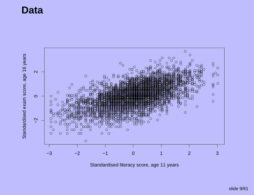
Data

−3 −2 −1 0 1 2 3

−2

02

Standardised literacy score, age 11 years

Sta

ndar

dise

d ex

am s

core

, age

16

year

s

slide 9/61

Plot of results age 16, 11 for each school

−0.8 −0.6 −0.4 −0.2 0.0 0.2 0.4 0.6

−1.

0−

0.5

0.0

0.5

1.0

Mean literacy of students entering a school age 11

Mea

n sc

hool

exa

m s

core

, age

16

slide 10/61

Example 2

471 patients with severe asthma randomised to receiveone of 4 levels of an active drug or placebo.

Each patient was allocated to one of 27 investigators.

Patients were followed up 2, 4, 8 & 12 weeks afterrandomisation; in addition they kept daily diaries.

FEV readings

Patients

Investigators

Level 1:

Level 2:

Level 3:

slide 11/61

Completion by treatment arm

Treatment group No. randomised No. completing

Placebo 91 38A, 100 mcg 91 72A, 200 mcg 92 84A, 400 mcg 99 88A, 800 mcg 98 90

slide 12/61

Data

0 2 4 6 8 10 12

12

34

5

Time from randomisation

FE

V1

(litr

es)

slide 13/61

Mean profiles

0 2 4 6 8 10 12

1.9

2.0

2.1

2.2

2.3

2.4

Weeks since randomisation

FE

V1

(litr

es)

placeboA, 100 mcgA, 200 mcgA, 400 mcgA, 800 mcg

slide 14/61

So

me

patien

tp

rofi

les

24

68

1012

1.0 2.0 3.0

FEV1 (litres) Patient: 5035

24

68

1012

1.0 2.0 3.0


24

68

1012

1.0 2.0 3.0


24

68

1012

1.0 2.0 3.0


24

68

1012

1.0 2.0 3.0


24

68

1012

1.0 2.0 3.0


24

68

1012

1.0 2.0 3.0


24

68

1012

1.0 2.0 3.0


24

68

1012

1.0 2.0 3.0


24

68

1012

1.0 2.0 3.0


24

68

1012

1.0 2.0 3.0


24

68

1012

1.0 2.0 3.0


24

68

1012

1.0 2.0 3.0


24

68

1012

1.0 2.0 3.0


24

68

1012

1.0 2.0 3.0


24

68

1012

1.0 2.0 3.0


24

68

1012

1.0 2.0 3.0


24

68

1012

1.0 2.0 3.0


24

68

1012

1.0 2.0 3.0


24

68

1012

1.0 2.0 3.0


slide15/61

Notation

Focus on two level data for now.

Let i ∈ (1, . . . I) index level 1 units (e.g. students),and j ∈ (1, . . . J) index level 2 units (e.g. schools).

Let yij be the response, with covariate xij .

We will use the (multivariate) normal distribution formodelling.

This is characterised by its mean and variance; our focuswill be on modelling the variance.

slide 16/61

Standard linear regression

A model for a straight line is

yij = β0 + β1xij + eij , eijiid∼N(0, σ2),

which assumes all level 1 units independent.

In other words, if we have I level 1 units for each of J leveltwo units, then writing

y′ = (y11, y21, . . . , yI1, y12, . . . , yI2, . . . , y1J , . . . , yIJ)′,

V y = σ2

1 0 0 . . . 0

0 1 0 . . . 0

0 0. . . . . . 0

0 0 . . . 1 0

0 0 . . . 0 1

, a IJ by IJ matrix.

slide 17/61

Problems when data are multilevel:

1. Standard errors are wrong

Hence so are hypothesis tests, p-values and confidenceintervals.

Subjects within a cluster (level 2 unit) are often similar toeach other, i.e. not independent. They therefore conveyless information about the value of a parameter than anindependent (unclustered) sample of the same size(Goldstein, 2003, p. 23).

Further, we would like to understand the sources ofvariability by modelling the variance. This is not possiblewith standard regression.

slide 18/61

Problems when data are multilevel:

2. Effect estimates can be misleading

Suppose we wish to relate literacy at age 11 to examresults at age 16.

An analysis which does not recognise the likely correlationbetween outcomes from students from the same schoolwill give equal weight to results from all students.

However, given that such correlation exists, and data areunbalanced (different numbers of students in differentschools) it will be better to give relatively more weight tochildren from smaller schools than larger schools.

slide 19/61

Multilevel model

Recall i—level 1 (e.g. student), j—level 2 (e.g. school).

Model: yij = xijβ + errorij.

So, Var yij = Var errorij, as mean x′ijβ constant.

Let y′j = (y1j , y2j , . . . , yIj) — the data for level 2 unit j.

Suppose this has I by I covariance matrix Σ.

The diagonal elements are Var[errorij],

The off diagonal elements are Cov[errorij , errori′j ].

slide 20/61

Block diagonal covariance matrix

The full data can then be written as a IJ length columnvector

y′ = (y′

1,y′2, . . . y

′J).

Key assumption: data from different level 2 units independent

This means the full covariance matrix of y is:

Σfull =

Σ 0 0 . . . 0

0 Σ 0 . . . 0

0 0. . . . . . 0

0 0 . . . Σ 0

0 0 . . . 0 Σ

.

slide 21/61

Unstructured model

We attempt to estimate every one of the I(I + 1)/2parameters in Σ.

For obvious reasons, this is known as an unstructuredcovariance matrix.

Provided we have enough data, this can work well fordesigned studies (where everyone is observed at the sametimes) such as the asthma trial.

For the educational data (and generally in epidemiologyand social sciences) where the children in each schoolhave very different literacy at age 11, it is a non-starter.

We therefore need to consider modelling the variance.

slide 22/61

Variance model

Key idea: Decompose errorij into three independentcomponents:

1. Person specific Random effects, denoted Uj

— captures differences between individuals.

2. Stationary correlation wij

— captures systematic local variation

3. Residual error— everything that’s left over.

So model becomes

yij = x′ijβ + z′

ijUj + wij + eij ,

andΣ = Σu + Σw + Σe.

slide 23/61

Residual error

Denote the residual error by eij .

Model eij ∼ N1(0,Ωe = σ2e), — ie all independent of each

other.

Write e′j = (eij, e2j , . . . , eIj), then ej ∼ NI(0,Σe), where

Σe = σ2e

1 0 0 . . . 0

0 1 0. . . 0

0 0. . . 1 0

0 0 . . . 0 1

is an I by I matrix.

slide 24/61

Random effects

Uj is d length row vector of level 2 (e.g. school) specificrandom effects.

Pre-multiply by d-length column vector zij to give impact oflevel-2 specific effect on observation i.

Example 1: Random intercepts:

Uj = u0j ∼ N(0, σ2u0), zij = 1 for all i.

Var(z′iju0j) = Var(u0j) = σ2

u0; Cov(z′iju0j , z

′i′ju0j) =

Cov(u0j , u0j) = σ2u0.

Thus Σu =

σ2u . . . σ2

u

.... . .

...σ2

u . . . σ2u

.

slide 25/61

Example 2: random intercepts and slopes

Uj =

(

u0j

u1j

)

∼ N

((

0

0

)

,

(

σ2u0 σu0,u1

σu0,u1 σ2u0

))

.

Then zij = (1, xij), so effect of random terms on school j atstudent i is

u0j + xiju1j .

Now,Var(z′

iju0j) = Var(u0j + xiju1j) = σ2u0 + x2

ijσ2u1 + 2xijσu0,u1;

Cov(z′iju0j , z

′i′ju0j) = Cov(u0j + xiju1j , u0j + xi′ju1j) =

σ2u0 + xijxi′jσ

2u1 + (xij + xi′j)σu0u1.

Hence Σu, which is rather messy!

slide 26/61

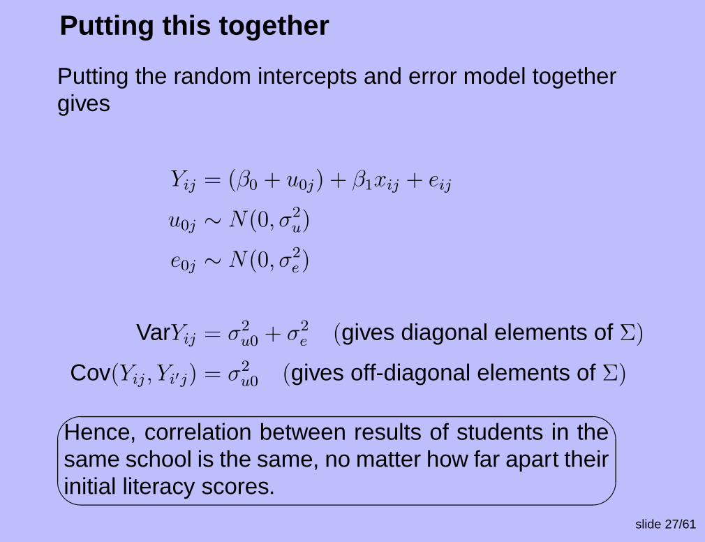
Putting this together

Putting the random intercepts and error model togethergives

Yij = (β0 + u0j) + β1xij + eij

u0j ∼ N(0, σ2u)

e0j ∼ N(0, σ2e)

VarYij = σ2u0 + σ2

e (gives diagonal elements of Σ)

Cov(Yij, Yi′j) = σ2u0 (gives off-diagonal elements of Σ)

Hence, correlation between results of students in thesame school is the same, no matter how far apart theirinitial literacy scores.

slide 27/61

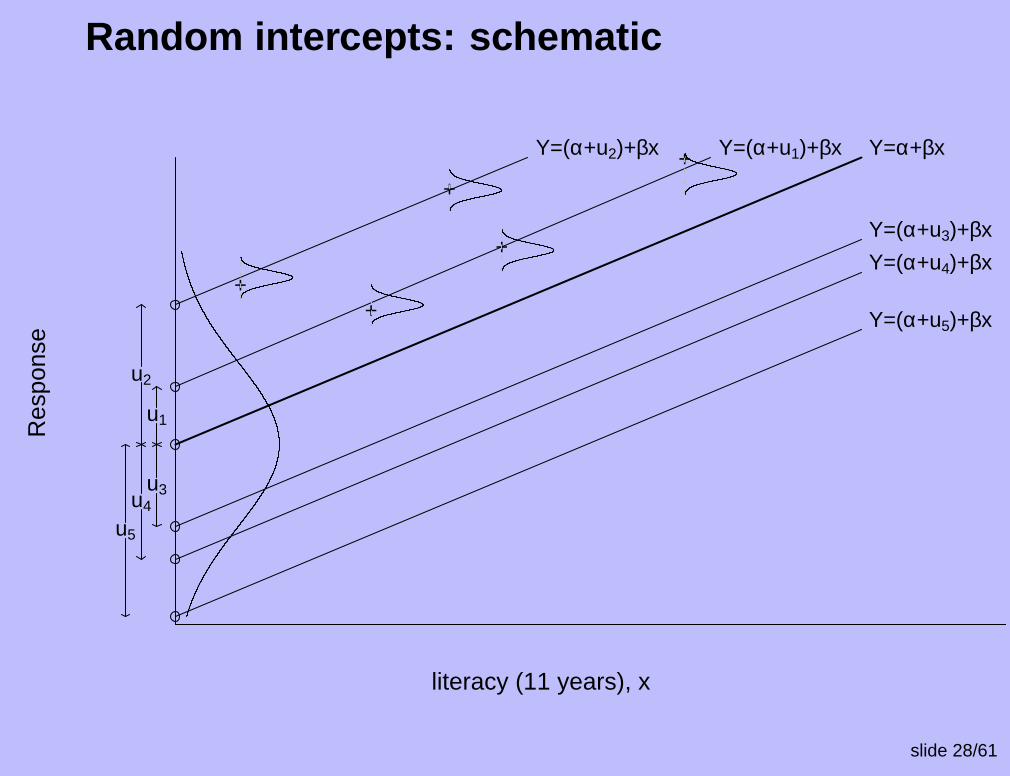
Random intercepts: schematic

literacy (11 years), x

Res

pons

e

+

+

+

+

+

Y=(α+u2)+βx Y=(α+u1)+βx Y=α+βx

Y=(α+u3)+βx

Y=(α+u4)+βx

Y=(α+u5)+βx

u1

u2

u3u4

u5

slide 28/61

And for random intercepts and slopes:

Yij = (β0 + u0j) + (β1 + u1j)xij + eij

(

u0j

u1j

)

∼ N

[(

0

0

)

,

(

σ2u0

σu0u1 σ2u1

)]

e0j ∼ N(0, σ2e)

VarYij = σ2u0 + x2

ijσ2u1 + 2σu0u1xij + σ2

e

(gives diagonal elements of Σ)

Cov(Yij , Yi′j) = σ2u0 + xijxi′jσ

2u1 + (xij + xi′j)σu0u1

(gives off-diagonal elements of Σ)

Now correlation between results of students in thesame school can decline as distance between theirliteracy scores increases.

slide 29/61

Random intercepts & slopes: schematic

literacy (11 years), x

Res

pons

eY=α+βxY=(α+u2)+(β + v2)x

Y=(α+u1)+(β + v1)x

Y=(α+u3)+(β + v3)x

Y=(α+u5)+(β + v5)x

Y=(α+u4)+(β + v4)x

(Note u0j ↔ uj ; u1j ↔ vj.)

slide 30/61

Fitting random intercepts model

slide 31/61

Plotting school level residuals

(Plot shows u0j ±√

2Var u0j)

slide 32/61

Interpretation

Can we deduce that schools at the right hand end arebetter - that they give students with the same 11 yearliteracy a better education? (jargon term: value added)

The UK department of Education does!

BUT

Our model assumed each school has the same slope: thisis equivalent to the correlation between students’ 16 yearresults in a school being the same, no matter how far aparttheir 11 year literacy.

Let’s fit a random intercepts and slopes model to test this.

slide 33/61

Random intercept & slope model

Log likelihood ratio test: 9357.3− 9316.9 = 40; cf χ22,

p = 2.1× 10−9.

slide 34/61

School specific slopes

(Note school lines do not extend out of range of theirstudents’ 11 year literacy intake)

slide 35/61

Interpretation

Picture is complex!

Some schools appear good for students with high literacyat 11, but less good for students with low literacy at 11. Forsome schools it is the reverse.

This may reflect specific teaching strategies.

Some schools are poor overall.

Use of a random intercepts model alone for these data ismisleading for parents and a disservice to schools.

Seehttp://www.mlwin.com/hgpersonal/league_tables_England_2004_commentary.htm

slide 36/61

Back to variance model

We decomposed Σ = Σu + Σw + Σu. Now consider Σw.

If Var yij increases (say with time), such as in growth data,the variance/covariance is non-stationary.

However, if the variance is constant over time and thecovariance depends only on the time betweenobservations, it is stationary.

We have seen that random effects (e.g. random interceptsand slopes) often give good models for non-stationaryprocesses.

However, they are not so good for stationary processes.Even if the variance is non-stationary, there may be astationary component.

slide 37/61

Stationary correlation structure

Again have w′j = (wij, w2j , . . . , wIj).

Recall trials example; see individuals repeatedly over timesi = 1, 2, . . . , I. A stationary covariance process has I by Imatrix Σw =

τ2

0

B

B

B

B

B

B

B

B

B

@

1 ρ(|1 − 2| = 1) . . . ρ(|1 − I| = I − 1)

ρ(|2 − 1| = 1) 1 . . . ρ(|2 − I| = I − 2)

...... . . .

...

ρ(|(I − 1) − 1| = I − 2) . . . 1 ρ(|(I − 1) − I| = 1)

ρ(|I − 1| = I − 1) . . . ρ(|I − (I − 1)| = 1) 1

1

C

C

C

C

C

C

C

C

C

A

where ρ(0) = 1, and ρ(|ω|)→ 0 as |ω| → ∞.

Forms for ρ( . ) include AR(1), exp(−α|ω|), · · ·

slide 38/61

Drawing it together

Recall trials example.For an individual with I measurements, theirvariance/covariance matrix is the I by I matrix

Σ = Σu + Σw + Σe,

Do we need these three components? Depends on dataset

• Some problems (typically growth) observationssufficiently spaced out that Σw = 0.

• Or, perhaps because of a standard manufacturingprocess association will be dominated by Σw andΣu = 0.

Remaining error, Σe 6= 0!

slide 39/61

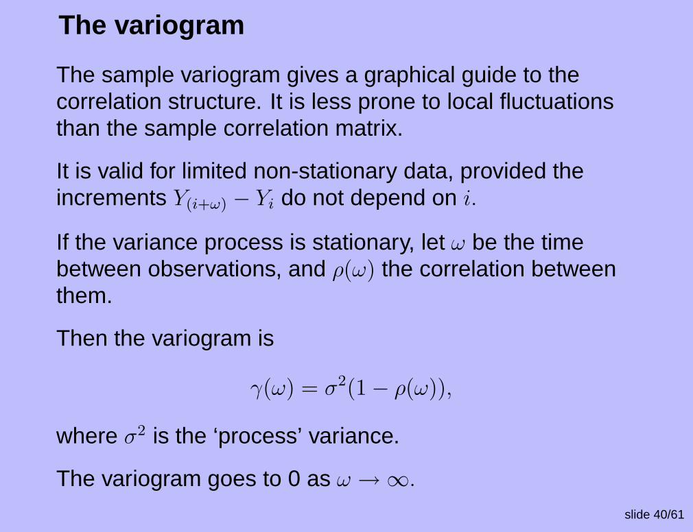
The variogram

The sample variogram gives a graphical guide to thecorrelation structure. It is less prone to local fluctuationsthan the sample correlation matrix.

It is valid for limited non-stationary data, provided theincrements Y(i+ω) − Yi do not depend on i.

If the variance process is stationary, let ω be the timebetween observations, and ρ(ω) the correlation betweenthem.

Then the variogram is

γ(ω) = σ2(1− ρ(ω)),

where σ2 is the ‘process’ variance.

The variogram goes to 0 as ω →∞.

slide 40/61

Estimating the variogram

Fit a ‘full’ model to the data, i.e. a model with the mostgeneral mean and variance structure you are interested in.

Calculate

1. the residuals, eij ;

2. the half-squared differences, νijk = 12(eij − eik)

2.

3. the corresponding time differences, δijk = tij − tik.

Then the sample variogram, γ(ω), is the average of all theνijk corresponding for which δijk = ω.

Finally, estimate the ‘process variance’ by the average of all

1

2(yij − ylk), for which i 6= l.

For more details see Diggle et al. (2002).slide 41/61

Interpreting the variogram

2

2

γ

random intercept variance

error variance

serial correlation

ω

(ω)

processvariance

σu2

σe

τ

slide 42/61

Application to asthma study

We estimate the variogram to guide the choice of variancemodel for the asthma study.

In designed studies, such as this, the choice ‘full model’ or‘unstructured model’ is fairly clear.

We fit a different mean for each treatment group at eachtime, and an unstructured covariance matrix.

We also fit a random term at a 3rd level — investigator.

slide 43/61

Asthma study: model

Let φil = 1 if patient i has treatment l = 1, . . . .5

We have observations at 2, 4, 8 & 12 weeks,corresponding to j = 1, 2, 3, 4.

Let k index investigator. The model is

yijk = φilβjl + uj + νk,

νk ∼ N(0, σ2ν)

u1

u2

u3

u4

∼ N(0,Σ), (unstructured; 10 parameters)

slide 44/61

Unstructured model for asthma data

slide 45/61

Estimated variogram

2 4 6 8 10

0.0

0.2

0.4

0.6

Weeks between observations, ω

γ(ω

)

Correlation virtually constant over time.Error variance ≈ 0.1.Random intercept variance ≈ 0.5.

slide 46/61

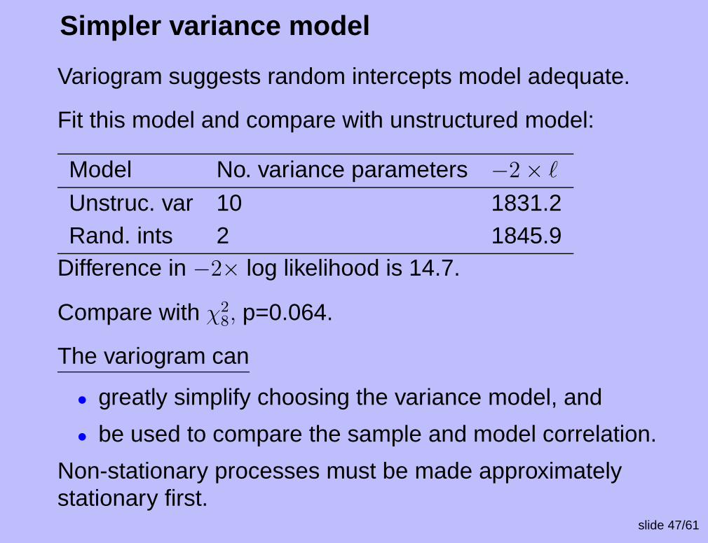
Simpler variance model

Variogram suggests random intercepts model adequate.

Fit this model and compare with unstructured model:

Model No. variance parameters −2× `

Unstruc. var 10 1831.2Rand. ints 2 1845.9

Difference in −2× log likelihood is 14.7.

Compare with χ28, p=0.064.

The variogram can

• greatly simplify choosing the variance model, and

• be used to compare the sample and model correlation.

Non-stationary processes must be made approximatelystationary first.

slide 47/61

Asthma study: fitted vs observed means

0 2 4 6 8 10 12

1.9

2.0

2.1

2.2

2.3

Weeks since randomisation

FE

V1

(litr

es)

raw datamodel Active, 100mcg

Placebo

Estimated means valid if data MAR.Borderline investigator effect vanishes after baseline adjustment.

slide 48/61

(Restricted) maximum likelihood

Our model is y ∼MN(Xβ,Σ),with log-likelihood −0.5log |Σ|+ (y −Xβ)′Σ−1(y−Xβ).

Maximise by direct Newton-Raphson search (e.g.Raudenbush and Bryk (2002), ch. 14). Often, iterativegeneralised least squares is faster (see below).

To correct the downward bias of ML estimators, use REMLlog-likelihood

−0.5log |Σ|+ (y −Xβ)′Σ−1(y −Xβ) + log |X ′Σ−1X|.

See, e.g. Verbeke and Molenberghs (2000), p. 43.

For moderately large data sets the results are similar,though in uncommon situations with many fixedparameters the two can give quite different answers(Verbeke and Molenberghs, 2000, p. 198).

slide 49/61

Testing

Changes in REML log-likelihoods cannot generally be usedto compare nested models unless X is unchanged. Somaximum likelihood may be preferred for model building(Goldstein, 2003, p. 36).

MLwiN always gives non-REML likelihood

Often Wald, or F-tests used for fixed effects, and likelihoodratio tests for random effects.

Asymptotically, fixed effects estimates (β) and varianceterm estimates independent; however, standard errors canbe too small in small data sets.

Kenward and Roger (1997) give an adjustment,implemented in SAS, for this.

slide 50/61

IGLS estimation

Goldstein (1986) showed how to maximise the multivariatenormal likelihood iteratively using two regressions.

Recall:

1. If yi = x′iβ + εi, εi

iid∼ N(0, σ2) then

β = (X ′X)−1X ′Y.

2. If yi = x′iβ + εi, εi not iid

∼ N(0, σ2) but Cov(Y ) = Σ,known

β = (X ′Σ−1X)−1X ′Σ−1Y.

slide 51/61

Model: Yij = β0 + β1xij + u0j + eij

EY =

1 x11

1 x21

......

1 xIJ

(

β0

β1

)

↑ ↑

X β

1. Guess Σ, ie guess Cov(Y ), setβ1 = (X ′Σ−1X)−1X ′Σ−1Y

2. Calculate residuals, R = Y −Xβ

3. IDEA Since E(RR′) = Σ, the covariance matrix of Y,create a regression model to estimate Σ.After estimating Σ, update β is step 1.

Iterate till convergenceslide 52/61

How do we estimate Σ?

E(R′R) =

r211 r12r11 . . .

r21r11 r222 . . .

.... . . . . .

=

σ2u0 + σ2

e σ2u0 . . .

σ2u0 σ2

u0 + σ2e . . .

.... . . . . .

So vec(R′R) =

r211

r21r11

...

=

1 1

0 1

1 1...

...

(

σ2e

σ2u0

)

+ ω

↑ Υ

← Zslide 53/61

Estimation of Σ (ctd)

A regression, BUT r’s not iid; turns out

Cov(vec(RR)) = Σ? = Σ⊗

Σ

ThusΥ = (Z ′Σ?−1Z)Z ′Σ?−1R

Full details in Goldstein and Rasbash (1992).

For discussion of residuals in multilevel modelling see, e.g.Robinson (1991).

slide 54/61

Software

Most packages offer software for continuous data.

Some comments on packages I have tried to use (noimplied judgment on other packages):

SAS, proc MIXED — the commercial airliner (expensive)

Excellent for fitting a wide range of standard models;provides a wide range of (stationary) covariance models.

Kenward-Roger adjustment to standard errors/degrees offreedom for small samples implemented (ddfm=kr). Notintuitive for beginners

Probably the best for regulatory pharma-industry analyses

slide 55/61

Software (ctd)

MLwin — the light aircraft (free to UK academics)

Fast, flexible multilevel modelling package — but you maycrash!

Fits an extremely wide range of models.

Very strong on random effects models; weak on stationarycovariance models.

Intuitive for teaching.

Stata (GLLAMM) — overland travel (∼ 200 USD)

Has a very general, but very slow, multilevel/latent variablemodelling package. A faster package for continuous datawith Stata 9.0.

slide 56/61

Software (ctd)

WinBUGS (free)

Very flexible package for model fitting using MCMC, withR/S+ like syntax.

I like to have a good idea what the answer is before I use it.

R (free)

Non-linear estimation package limited compared with SASand MLwiN;

Trellis graphics and data manipulation awkward.

Syntax hard for teaching

For up-to-date reviews (re)-visit www.mlwin.com

slide 57/61

Summary

• Once you look, multilevel structure is everywhere.

• This is an important aspect of the data; ignoring itleads to misleading results.

• Distinguish between the mean model and thecorrelation model; understand the impact of randomeffects models on the correlation.

• Estimation: REML is usually preferable. Don’t usechanges in REML likelihood for fixed effects inference,though.

• Get started using the tutorial material athttp://tramss.data-archive.ac.uk/Software/MLwiN.asp

• Further references: see Carpenter (2005).

slide 58/61

References

Carpenter, J. R. (2005) Multilevel models. InEncyclopaedic Companion to Medical Statistics (EdsB. Everitt and C. Palmer). London: Hodder andStoughton.

Diggle, P. J., Heagerty, P., Liang, K.-Y. and Zeger, S. L.(2002) Analysis of longitudinal data (second edition).Oxford: Oxford University Press.

Goldstein, H. (1986) Multilevel mixed linear model analysisusing iterative generalized least squares. Biometrika, 73,43–56.

Goldstein, H. (2003) Multilevel statistical models (secondedition). London: Arnold.

slide 59/61

References

Goldstein, H. and Rasbash, J. (1992) Efficientcomputational procedures for the estimation ofparameters in multilevel models based on iterativegeneralised least squares. Computational Statistics andData Analysis, 13, 63–71.

Kenward, M. G. and Roger, J. H. (1997) Small sampleinference for fixed effects from restricted maximumlikelihood. Biometrics, 53, 983–997.

Raudenbush, S. W. and Bryk, A. S. (2002) Hierarchicallinear models: applications and data analysis methods(second edition). London: Sage.

Robinson, G. K. (1991) That BLUP is a good thing: theestimation of random effects. Statistical Science, 6,15–51.

slide 60/61

References

Verbeke, G. and Molenberghs, G. (2000) Linear MixedModels for Longitudinal Data. New York: Springer Verlag.

slide 61/61

II: Extensions

• Multilevel models for discrete data• Marginal vs Conditional models• Example: clinical trial• Estimation issues• Software

• Models for cross-classified data• Notation• Example: Scottish educational data

• Models for multiple membership cross-classified data• Notation• Example: Danish poultry farming

slide 1/53

Review: random intercepts

Suppose j indexes subjects (level 2) and i indexesrepeated observations (level 1).

Recall the random intercepts model:

yij = (β0 + uj) + β1xij + eij

uj ∼ N(0, σ2u)

eij ∼ N(0, σ2e).

If yij is now binary, a natural generalisation is

logit Pr(yij = 1) = (β0 + uj) + β1xij

u0i ∼ N(0, σ2u)

slide 2/53

Interpretation

In the previous model logit Pr(yij = 1) is reallylogit Pr(yij = 1|xij , uj).

Thus, this is a Subject Specific (SS) model;β is the log-odds ratio of the effect of x for a specific uj .

We can also construct Population Averaged (PA) models

logit Pr(yij = 1|xij) = βp0 + βp

1xij

Define expit as the inverse logit function. Then

Euexpit(β0 + β1xij + uj) 6= expit(β0 + β1xij).

So PA estimates do not equal SS estimates.

The exception is the normal model, where expit is replacedby the identity.

slide 3/53

Interpretation (ctd)

Let β denote SS estimates, βp PA estimates. In general

• |βp| < |β|, with equality if σ2u = 0.

• If σ2u is large, the two will be very different.

Exampleyij indicates coronary heart disease for subject j at time ix1ij indicates the subject smokesx2ij indicates one of their parents had CHD

βp1 : effect of smoking on log-odds of CHD in population

β1 : effect of stopping smoking for a given subject

βp2 : Effect of parental CHD in the population

β2 : Effect of change in parental CHD for given individual ??

slide 4/53

Choosing between PA and SS

It depends on the question:SS more appropriate when population averaged effects areimportant:

• In epidemiology & trials, where we are interested in theaverage effect of treatment on a population

• In education, when we are interested in the averageeffects of interventions across populations

BUT: the same process in two populations with differentheterogeneity will lead to different βp.

SS preferable for

• Estimating effects on individuals, schools

• Modelling sources of variability.

slide 5/53

Example: Clinical trial

241 patients randomised to receive either a placebo oractive treatment.

Three treatment periods.

In each period, each patient undergoes a series of tests(the number varying between patients).

Each test has a binary response (1=success).

Dropout Treatment groupPlacebo Active

Period 1 0 0Period 2 10 5Period 3 25 12Completers 82 107

slide 6/53

No. of tests by period and intervention

Period 1 Period 2 Period 3 Period 1 Period 2 Period 3

1020

3040

Placebo Treatment Active Treatment

slide 7/53

SS models

Let k index patient, j period and i test, and δk = 1 if patientk has active treatment. A general model is

Eyijk = µjk,

expit(µjk) = αj + δkβj + basekγj + ωjk,

where either:(i) ωjk = uk, uk ∼ N(0, σ2

u) — random intercepts

(ii) ωjk = (u0k + u1ktj), (u0k, u1k) ∼ N2(0,Ω) — randomintercepts and slopes

(iii) ωjk = ujk and

u1k

u2k

u3k

∼ N

0

0

0

,

σ2u1

σu0u2σ2

u2

σu1u3σu2u3

σ2u3

.

slide 8/53

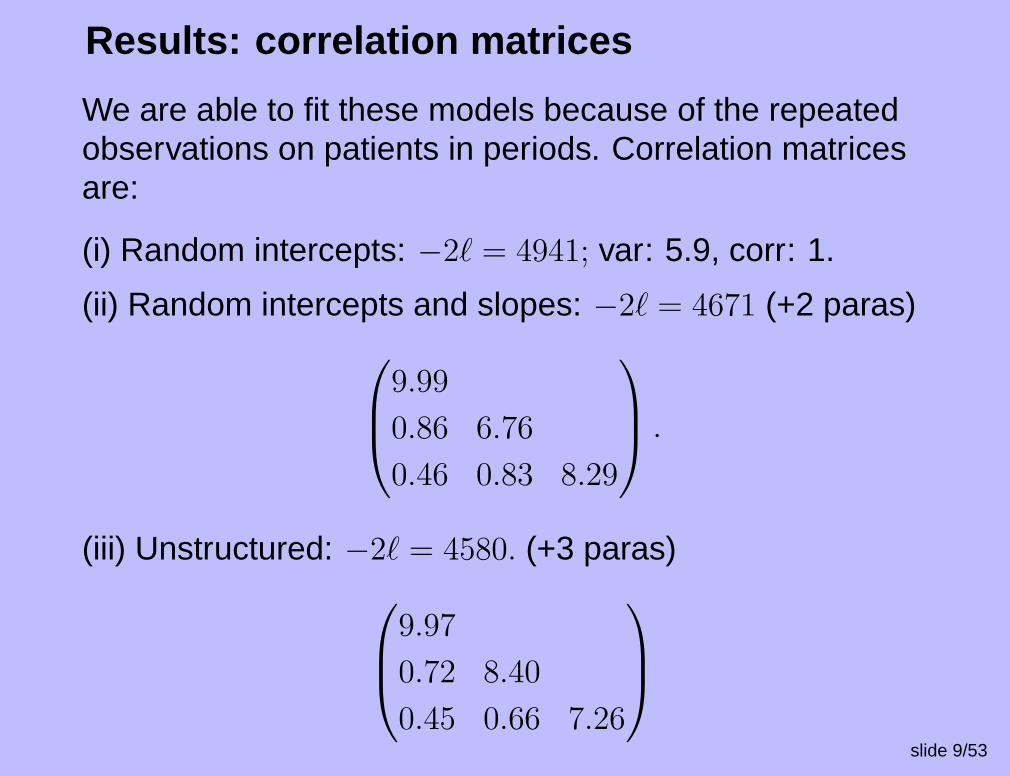
Results: correlation matrices

We are able to fit these models because of the repeatedobservations on patients in periods. Correlation matricesare:

(i) Random intercepts: −2` = 4941; var: 5.9, corr: 1.

(ii) Random intercepts and slopes: −2` = 4671 (+2 paras)

9.99

0.86 6.76

0.46 0.83 8.29

.

(iii) Unstructured: −2` = 4580. (+3 paras)

9.97

0.72 8.40

0.45 0.66 7.26

slide 9/53

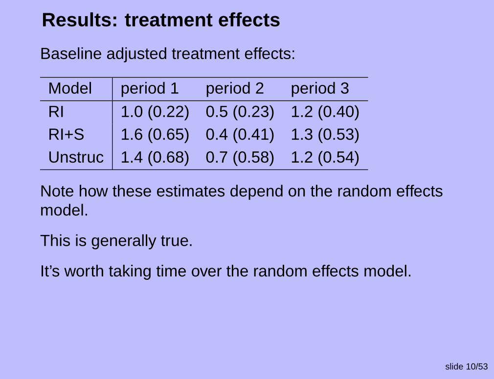
Results: treatment effects

Baseline adjusted treatment effects:

Model period 1 period 2 period 3

RI 1.0 (0.22) 0.5 (0.23) 1.2 (0.40)RI+S 1.6 (0.65) 0.4 (0.41) 1.3 (0.53)Unstruc 1.4 (0.68) 0.7 (0.58) 1.2 (0.54)

Note how these estimates depend on the random effectsmodel.

This is generally true.

It’s worth taking time over the random effects model.

slide 10/53

Getting PA coefficients from SS ones

Sometimes it is useful to obtain PA estimates from SSones (NB can’t go the other way!).

This is particularly easy when we have a designed study,so that the coefficients for the random terms in the modelare the same for each patient at each time.

For simplicity we need to estimate the mean at each time,rather than fitting a slope across time. As before the modelis:

Eyijk = µjk,

h(µjk) = αj + δkβj + basekγj + z′juk

uk ∼ N(0,Σu).

The table below, derived from Zeger et al. (1988), showshow to obtain the PA coefficients.

slide 11/53

Table for obtaining PA from SS effects

Link function, h( . ) Random intercepts,zj = 1 General random structure zj

log αpj = αj + σ2

u/2 αpj = βj + z′

jΣuzj/2

βp

j = βj βp

j = βj

γp

j = γj γp

j = γj

probit αp

j = αj/√

1 + σ2u α

p

j = αj/√

|I + Σzjz′

j |

βpj = βj/

√

1 + σ2u β

pj = βj/

√

|I + Σzjz′

j |

γpj = γj/

√

1 + σ2u γ

pj = γj/

√

|I + Σzjz′

j |

logistic αp

j ≈ αj/√

1 + 0.34584σ2u α

p

j ≈ αj/√

|I + 0.34584Σzjz′

j |

βp

j ≈ βj/√

1 + 0.34584σ2u β

p

j ≈ βj/√

|I + 0.34584Σzjz′

j |

γp

j ≈ γj/√

1 + 0.34584σ2u γ

p

j ≈ γj/√

|I + 0.34584Σzjz′

j |

slide 12/53

Accuracy of logistic approximation

−4 −2 0 2 4

−4

−2

02

4

ηp

η(1

+0.

3458

4×

σ2 )0.5

σ2 = 1σ2 = 8σ2 = 16

slide 13/53

Example

We use data from period 3 of the trial described above,and fit a random intercepts model with (i) probit link and (ii)logistic link.

We compare using the transformation with fitting anindependence GEE (=GLM here) with robust SEs.

Link GLM estimates Transformed SS SSestimates estimates

probit 0.323 (0.190) 0.318 (0.167) 0.544 (0.285)logit 0.636 (0.407) 0.577 (0.301) 1.100 (0.573)

For the logistic model σ2u = 7.6.

Agreement improves as sample size increases.

slide 14/53

Using simulation to obtain PA estimates

Sometimes it is easier to use simulation. Consider therandom intercepts model:

1. Fit the model. Draw M values of the SS random effectfrom from N(0, σ2

u) : u1, . . . , uM .

2. For m = 1, . . . ,M and for a particular x, compute

πm = expit(β0 + β1x + z′um)

3. Mean (population averaged) probability is

πp =1

M

M∑

m=1

πm.

slide 15/53

Estimation: PA models

If Var(yj) were known, we could use the score equation forβ when the data follow a log-linear model:

s(β) =

J∑

j=1

(

∂µj

∂β

)

Var(yj)−1(yj − µj) = 0.

Liang and Zeger (1986) showed that if we write Var(yj) asVar(yj, β, α), then if we use any

√J-consistent estimator

for α, the estimates of β obtained by solving this areasymptotically as efficient as those we would get were αknown.

In practice, usually an estimating equation for α is formedand the resulting Generalised Estimating Equations(GEEs) solved simultaneously (e.g. Prentice (1988)).

slide 16/53

GEEs: notes on estimation

• β is nearly efficient relative to ML estimates providedVar[Eyj ] is reasonably approximated.

• β is consistent as J → ∞ even if the covariancestructure of yj is incorrect.

• Once the mean model is chosen, the robustness ofinferences can be checked by trying variouscovariance structures, and comparing the parameterestimates and their robust standard errors.

• As GEEs are moment-based estimators, they areinvalid with missing data, unless it is missingcompletely randomly.

Further details in Diggle et al. (2002).

slide 17/53

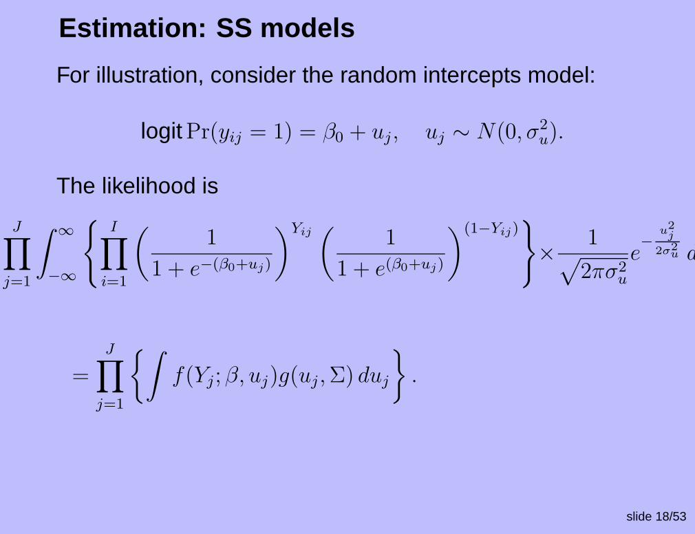
Estimation: SS models

For illustration, consider the random intercepts model:

logit Pr(yij = 1) = β0 + uj , uj ∼ N(0, σ2u).

The likelihood is

J∏

j=1

∫ ∞

−∞

I∏

i=1

(

1

1 + e−(β0+uj)

)Yij(

1

1 + e(β0+uj)

)(1−Yij)

× 1√

2πσ2u

e−

u2

j

2σ2u duj

=J∏

j=1

∫

f(Yj;β, uj)g(uj ,Σ) duj

.

slide 18/53

Obtaining parameter estimates

The likelihood for individual j is

L(β, σ2u|Yj) =

∫

f(Yj|uj , β)g(uj , σ2u) duj .

When f, g normal this integral is the multivariate normaldistribution of the data, maximised as described insession 1.

Otherwise, the integral is intractable. Options are

• Numerical integration (e.g. SAS NLMIXED)(slow for many random effects)

• Quasi likelihood methods

slide 19/53

Penalised Quasi-likelihood

Consider observation ij, and drop subscripts:

y = µ(η) + ε = expit(Xβ + Zu) + ε.

After update t, have βt, ut, say. Expand about true β, u :

yij ≈ µ(Xβt + Zut) +∂µ

∂ηX(β − βt) +

∂µ

∂ηZ(u − ut) + ε.

Re-arrange:

y − µ(Xβt + Zut) +∂µ

∂ηXβt +

∂µ

∂ηZut =

∂µ

∂ηXβ +

∂µ

∂ηZu + ε.

I.e. y? = X?β + Z?u + ε.

Constrain Var ε = µ(1 − µ), and obtain new estimates with1 step of fitting routine for normal data.

slide 20/53

Comments on quasi-likelihood methods

• Estimation at almost the same speed as for normalmodels.

• No estimate of the log-likelihood.

• Estimates can be badly biased if– fitted values close to 0 or 1– some individuals have few observations

• Obvious solution is to try the 2nd order Taylorexpansion — called PQL(2)– bias is substantially reduced, but can’t always be

fitted

• There have been various proposals forsimulation-based bias correction.

Ng et al. (2005) consider these, and concludeSimulated Maximum Likelihood (SML) is best.

slide 21/53

SML method for bias correction

Recall likelihood: L(β,Σ|y) =∫

f(y|u, β)g(u,Σ) du.

Obtain initial estimates β, Σ, from PQL(2). Set Σ = Σ. Then

L(β,Σ) =

∫

f(y|u, β)g(u,Σ)g(u, Σ)

g(u, Σ)du

≈ 1

H

H∑

h=1

f(y|uh, β)g(uh,Σ)

g(uh, Σ)

where u1, . . . , uhiid∼g(u, Σ).

Search for β,Σ that maximise this Monte-Carlo likelihoodestimate (keeping Σ fixed).

slide 22/53

Simulation study

Compare PQL (2) followed by SML with SAS procNLMIXED.

Use example of Kuk (1995). Simulate 100 data sets from

Yij ∼ bin(6, πij

logit(πij) = 0.2 + uj + 0.1xij

uj ∼ N(0, 1)

J = 15 level 2 units with I = 2 level 1 units each.

x = −15,= 14, . . . , 14.

slide 23/53

Results

Values are average estimates (Mean Squared Error)

Parameter β0 β1 σ2

True values 0.2 0.1 1SML (H=500) 0.203 0.099 0.939

(0.136) (0.00134) (0.561)SAS NLMIXED 0.190 0.097 0.927

(0.135) (0.00134) (0.478)NLMIXED needs starting values: gave 0 for β0, β1 and 1 for σ2.NLMIXED had convergence problems on 17/100 data sets: these are excluded.

Conclude(i) SAS NLMIXED larger bias, smaller variance; BUT weonly used H=500(ii) PQL(2) + SML seems to work well.

slide 24/53

Example: Bangladesh data

A sub-sample of the 1988 Bangladesh fertility surveyHuq and Cleland (1990).

All the women had been married at some time.

i = 1, . . . , 1934 women (level 1) from j = 1, . . . , 60 districts(level 2).

2–118 women in each district.

Response: yij =

1 if the women reported contraceptive use0 otherwise

.

Covariates: urban resident; age; no. of children

slide 25/53

Model

Let 1[ ] is an indicator for the event in brackets.

The model is:

logitPr(Yij = 1) = (β0 + u0j) + (β1 + u1j) × 1[urban resident]

+ β2 × (centred age) + β3 × 1[1 child]

+ β4 × 1[2 children] + β5 × 1[≥ 3 children],

(

u0j

u1j

)

∼ N

(

0

0

)

,

(

σ2u0

σu0u1 σ2u1

)

.

slide 26/53

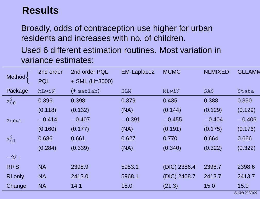
Results

Broadly, odds of contraception use higher for urbanresidents and increases with no. of children.Used 6 different estimation routines. Most variation invariance estimates:

2nd order 2nd order PQL EM-Laplace2 MCMC NLMIXED GLLAMMMethod

PQL + SML (H=3000)

Package MLwiN (+ matlab) HLM MLwiN SAS Stata

σ2

u00.396 0.398 0.379 0.435 0.388 0.390

(0.118) (0.132) (NA) (0.144) (0.129) (0.129)

σu0u1 −0.414 −0.407 −0.391 −0.455 −0.404 −0.406

(0.160) (0.177) (NA) (0.191) (0.175) (0.176)

σ2

u10.686 0.661 0.627 0.770 0.664 0.666

(0.284) (0.339) (NA) (0.340) (0.322) (0.322)

−2` :

RI+S NA 2398.9 5953.1 (DIC) 2386.4 2398.7 2398.6

RI only NA 2413.0 5968.1 (DIC) 2408.7 2413.7 2413.7

Change NA 14.1 15.0 (21.3) 15.0 15.0slide 27/53

Implications: software

• HLM v6: EM-Laplace2: No SE estimated for randomcomponents. In another problem, estimated randomcomponents are smaller than estimates fromSML/NLMIXED.

• HLM v5: Laplace6: convergence problems.

• GLLAMM is slow

• MCMC (Gamma diffuse priors on variances) givesinflated estimates, relative to ML.

• NLMIXED needs starting values (here from PQL(2))

• SML appears to work well

Conclude:PQL(2) plus SML or NLMIXED for ‘bias correction’ usuallygives best answers.

slide 28/53

Cross classified data

So far we have considered only hierarchical structures.

However, social structures are not always hierarchical.People often belong to more than one grouping at a givenhierarchical level.

E.g. neighbourhood and school may both have effects oneducational outcomes:

– a school may contain children from severalneighbourhoods;

– children from one neighbourhood may attend differentschools

Children are nested in a cross classification ofneighbourhood and school.

slide 29/53

Classification diagrams

School

Children

Neighbourhood N1 N2 N3

S1 S2 S3 S4

C1 C2 C3 C4 C5 C6 C7 C8 C9 C10

Neighbourhood

School

Pupil

Neighbourhood School

PupilNested structure Cross classified structure

slide 30/53

Standard notation

Yi(j1j2) is the response for pupil i in neighbourhood j1 andschool j2.

The subscripts j1 and j2 are bracketed together to indicatethat these classifications are at the same level, i.e. pupilsare nested within a cross-classification of neighbourhoodsand schools.

A basic cross-classified model may be written:

yi(j1j2) = β′xi(j1j2) + u1j1 + u2j2 + ei(j1j2).

u1j1 is the random neighbourhood effect

u1j2 is the random school effect

slide 31/53

Alternative notation

For hierarchical models we have one subscript per level,and nesting is implied by reading from left to right.

E.g. ijk denotes the ith level 1 unit within the jth level 2unit within the kth level 3 unit.

For cross-classified models, we can group together indicesfor classifications at the same level using parentheses (seeprevious slide). However, having one subscript perclassification becomes cumbersome.

Using an alternative notation, we have a single subscript,no matter how many classifications there are.

slide 32/53

Data matrix for cross-classification

Single subscript notation.

Let i index children.i Neighbourhood(i) School(i)

1 1 12 2 13 1 14 2 25 1 26 2 37 2 38 3 39 3 4

10 2 4

slide 33/53

Cross classified model

Using the single-subscript notation, yi is the outcome forchild i.

Classification1 is child, 2 is neighbourhood and 3 is school.

yi = β′xi + u(2)nbhd(i) + u

(3)sch(i) + ei

u(2)nbhd(i) ∼ N(0,Ω

(2)u ) Random departure due to neighbourhood

u(3)sch(i) ∼ N(0,Ω

(3)u ) random departure due to school

ei ∼ N(0,Ωe) individual-level residual

Covariates may be defined for any of the 3 classifications

Coefficients may be allowed to vary across neighbourhoodor school.

slide 34/53

Cross-classified model: notation

From the previous slide, the model is:

yi = β′xi + u(2)nbhd(i) + u

(3)sch(i) + ei.

Thus, for pupils 1 and 10 in the data set 2 slides back,

y1 = β′x1 + u(2)1 + u

(3)1 + e1;

y10 = β′x10 + u(2)2 + u

(3)4 + e10.

slide 35/53

Other cross-classified structures

• Pupils within primary schools by secondary schools

• Patients within GPs by hospitals

• Survey respondents within sampling clusters byinterviewers

• Repeated measures within raters by individuals(e.g. patients by nurses)

• Students following modular degree courses, e.g.Simonite and Browne (2003)

slide 36/53

Example: Scottish school children

3435 children who attended 148 primary schools and 19secondary schools in Fife, Scotland.

Classifications: 1 – student; 2 – primary school; 3 –secondary school

yi – overall achievement at age 16 for student i

xi – verbal reasoning at age 12 (mean centred)

2-level cross classified model:

yi = β0 + β1xi + u(2)prim(i) + u

(3)sec(i) + ei

slide 37/53

Results

Hierarchical Cross-classifiedmodel model

Fixedβ0 5.99 5.98β1 0.16 (0.003) 0.16 (0.003)Randomσ

(2)u (primary) — 0.27 (0.06)

σ(3)u (secondary) 0.28 (0.06) 0.01 (0.02)

σe (student residual) 4.26 (0.10) 4.25 (0.10)

Most of the variation in results at 16 years can be attributedto primary schools — an intriguing result for educationalresearchers overlooked without a cross-classified model.

slide 38/53

Cross-classification: covariance matrix

Recall in our hierarchical model, the covariance matrix wasblock diagonal:

Σfull =

Σ 0 0 . . . 0

0 Σ 0 . . . 0

0 0. . . . . . 0

0 0 . . . Σ 0

0 0 . . . 0 Σ

.

With a cross classified model this is no longer true.

E.g. for our example, suppose we first classify pupils withinsecondary schools.

For every student who shares a primary school with astudent from another secondary school, there is an offdiagonal term — Ω(2) (primary).

slide 39/53

Estimation

This makes ML estimation much harder.

Provided the cross-classification is not too widespread,careful ordering of the data can cause the covariancematrix to consist of —much larger— diagonal blocks.

Consequently, estimation is much more memory intensive,and much slower.

MCMC estimation in MLwiN is much more efficient.

See the manual MCMC Estimation in MLwiN by W Browne,downloadable from www.mlwin.com

slide 40/53

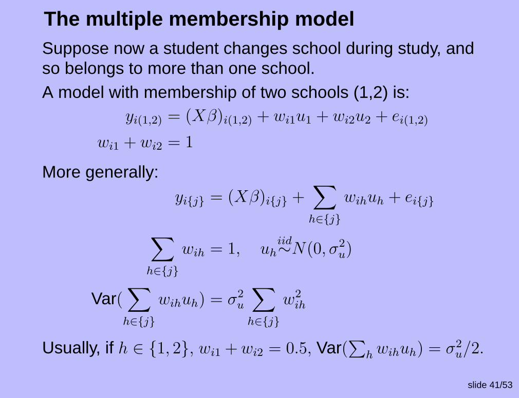
The multiple membership modelSuppose now a student changes school during study, andso belongs to more than one school.A model with membership of two schools (1,2) is:

yi(1,2) = (Xβ)i(1,2) + wi1u1 + wi2u2 + ei(1,2)

wi1 + wi2 = 1

More generally:yij = (Xβ)ij +

∑

h∈j

wihuh + eij

∑

h∈j

wih = 1, uhiid∼N(0, σ2

u)

Var(∑

h∈j

wihuh) = σ2u

∑

h∈j

w2ih

Usually, if h ∈ 1, 2, wi1 + wi2 = 0.5, Var(∑

h wihuh) = σ2u/2.

slide 41/53

Example: Danish poultry farming

Interested in understanding variation in salmonellaoutbreaks in chicken flocks.

Data from salmonella outbreaks in flocks of chickens inDanish poultry farms between 1995 & 1997.

Response is whether or not a ‘child flock’ was infected.

There are two hierarchies in the data: a productionhierarchy and a breeding hierarchy.

Full details:Browne et al. (2001)

slide 42/53

Production hierarchy

Level 1 units are child flocks of chickens.

Child flocks live for only a short time (∼35 days) beforethey are slaughtered for consumption.

Child flocks are kept in houses; in a year a house mayhave a throughput of 10–12 flocks.

Houses are grouped in farms.

Data from 10,127 child flocks, 725 houses, 304 farms.

slide 43/53

Breeding hierarchy

There are 200 parent flocks.

Eggs are taken from parent flocks to 4 hatcheries.

After hatching, chicks are transported to the farms in theproduction hierarchy (previous slide).

Child flocks draw chicks from up to six parent flocks.

slide 44/53

Classification diagram

Production farm

House

Child flock

Parent flock

h1 h2 h1 h2

p1 p2 p5p4p3

f1 f2

Each child flock connected to multiple parent flocks, sochild flocks are multiple members of parent flocks.Parental membership information is known.

Parent flocks are also cross-classified with the house/farmproduction hierarchy.

slide 45/53

Questions

To what extent is variability in child flock infectionattributable to

• production processes (hygiene on houses and farms)?

• hatcheries processes?

• parent flock processes– genetic predisposition to salmonella?– poor parent flock hygiene introducing infected eggs

into the system?

slide 46/53

Model: notation

Let πI = Pr(flock i has salmonella).

Let 1[96], 1[97] indicate data from 1996, 1997.

Let 1[hatch1], . . . , 1[hatch4] indicate the four hatcheries inwhich all the eggs form the parent flocks are hatched.

Let p.flock(i) be the set of parent flocks for child flock i.

We know the exact makeup of each child flock (in terms ofparent flocks). Define weights for each child flock i, wij, torepresent this makeup.

For each child flock, i, these satisfy∑

j∈p.flock(i)

wij = 1

slide 47/53

Model: components of variance

logitπi =β0 + β1 × 1[96] + β2 × 1[97]

+ β3 × 1[hatch2] + β4 × 1[hatch3] + β5 × 1[hatch4]

+ u(2)

house(i)+ u

(3)

farm(i)+

∑

j∈p.flock(i)

wiju(4)j

u(2)

house(i)∼ N(0, σ2

(2))

u(3)

farm(i)∼ N(0, σ2

(3))

u(4)j ∼ N(0, σ2

(2))

u(2) ⊥ u(3) ⊥ u(4)

slide 48/53

ResultsEstimation: PQL unstable; used MCMC

Description Estimate SE

intercept −1.86 0.187

1996 −1.04 (0.131

1997 −0.89 0.151

hatchery 2 −1.47 0.22

hatchery 3 −0.17 0.21

hatchery 4 −0.92 0.29

parent flock variance 1.02 0.22

farm variance 0.59 0.11

house variance 0.19 0.09

ConcludeSome hatcheries better than others;variability dominated by parent flock.

slide 49/53

Summary

• Extended ideas of session 1 to multilevel discrete data.

• Contrasted subject-specific and population-averagedmodels.

• Described random-effects models for discrete data.

• Discussed estimation & software issues for SS models.

• Extended ideas to cross-classified and multiplemembership models.

• Such models can be fitted in MLwiN, with care.

• More examples and documentation at www.mlwin.com

slide 50/53

References

Browne, W. J., Goldstein, H. and Rasbash, J. (2001)Multiple membership multiple classification (mmmc)models. Statistical modelling, pp. 103–124.

Diggle, P. J., Heagerty, P., Liang, K.-Y. and Zeger, S. L.(2002) Analysis of longitudinal data (second edition).Oxford: Oxford University Press.

Huq, N. M. and Cleland, J. (1990) Bangladesh FertilitySurvey 1989: (Main Report). Dhaka: National Institute ofPopulation Research and Training.

Kuk, A. Y. C. (1995) Asymptotically unbiased estimation ingeneralized linear models with random effects. Journal ofthe Royal Statistical Society, Series B (statisticalmethodology), 57, 395–407.

slide 51/53

References

Liang, K.-Y. and Zeger, S. L. (1986) Longitudinal dataanalysis using generalized linear models. Biometrika, 73,13–22.

Ng, E. S. W., Carpenter, J. R., Goldstein, H. and Rasbash,J. (2005) Estimation in generalised linear mexed modelswith binary outcomes by simulated maximum likelihood.

Prentice, R. L. (1988) Correlated binary regression withcovariates specific to each binary observation.Biometrics, pp. 1033–1048.

Simonite, V. and Browne, W. J. (2003) Estimation of a largecross-classified multilevel model to study academicachievement in a modular degree course. Journal of theRoyal Statistical Society, series A, Statistics in Society,116, 1–15.

slide 52/53

References

Zeger, S. L., Liang, K.-Y. and Albert, P. S. (1988) Modelsfor longitudinal data: a generalized estimating equationapproach. Biometrics, 44, 1049–1060.

slide 53/53

applied multilevel modelling â€” an introduction

Documents