applied mathematics and computer science …applied mathematics and computer science collaborations...

Applied Mathematics andApplied Mathematics andComputer Science CollaborationsComputer Science Collaborationsin in TerascaleTerascale Accelerator ModelingAccelerator Modeling

Esmond G. Ng([email protected])

Lawrence Berkeley National Laboratory

1

TerascaleTerascale Accelerator ModelingAccelerator Modeling

q Three components in the Accelerator SciDAC Project.§ Beam Systems Simulations (R. Ryne, LBNL).§ Electromagnetic Systems Simulations (K. Ko, SLAC).§ Advanced Accelerator Systems Simulations (W. Mori, UCLA).

q One of the SciDAC goals is to encourage interactions and collaborations between application scientists and applied mathematicians/computer scientists to advance large-scale high-performance simulations.§ Lots of opportunities in this accelerator project.

2

SciDACSciDAC ISIC’sISIC’s and SAPPand SAPP

q SciDAC Integrated Software Infrastructure Centers (ISIC’s) provide the expertise in applied math and computer science.§ APDEC – Algorithmic and Software Framework for Applied PDEs.§ TOPS – Terascale Optimal PDE Simulations.§ TSTT - Terascale Simulation Tools and Technology.§ CCTTSS – Component Technology for Terascale Simulation

Software.§ PERC – Performance Evaluation Research.

q SciDAC Scientific Application Pilot Program (SAPP) provides the linkage between ISIC’s and applications (in most cases).§ BNL, LANL, LBNL, Stanford, UC Davis.

3

ISIC and SAPP ActivitiesISIC and SAPP Activities

q Linear Algebra – large-scale sparse eigensolvers, sparse linear equations solvers (LBNL, Stanford, SLAC).

q Load Balancing (LBNL, SLAC).q Adaptive Mesh Refinements – particle-in-cell simulations and

advanced accelerators (LBNL).q Meshing – long-term stability in unstructured finite element

meshes (SLAC, SNL) and unstructured mesh refinement (RPI).q Visualization - visualization & animation of large datasets (UC

Davis, SLAC, LBNL).q Statistical Methods (LANL, LBNL).q Wake Field Modeling – modeling interaction of particle beams

with wake fields in high-intensity accelerators (BNL).

4

OutlineOutline

q Electromagnetic Systems§ Omega3P§ Tau3P§ Visualization

q Beam Systems and Advanced Accelerators§ Visualization§ Particle-in-cell simulations§ Gas jet calculations§ Statistical methods

5

CS/AM Efforts Related To Omega3PCS/AM Efforts Related To Omega3P

q Omega3P calculates cavity mode frequencies and field vectors.

§ Large-scale Eigenvalue/Eigenvector Calculations.• G. Golub, Y. Sun (Stanford) – SAPP.• P. Husbands, S. Li, E. Ng, C. Yang (LBNL) – TOPS & SAPP.

§ Parallel Adaptive Mesh Refinement.• I. Malik (Stanford), Z. Li (SLAC) – Accelerator Project.• Y. Luo, M. Shephard (RPI) – TSTT.

6

LargeLarge--scale scale EigenvalueEigenvalue CalculationsCalculations

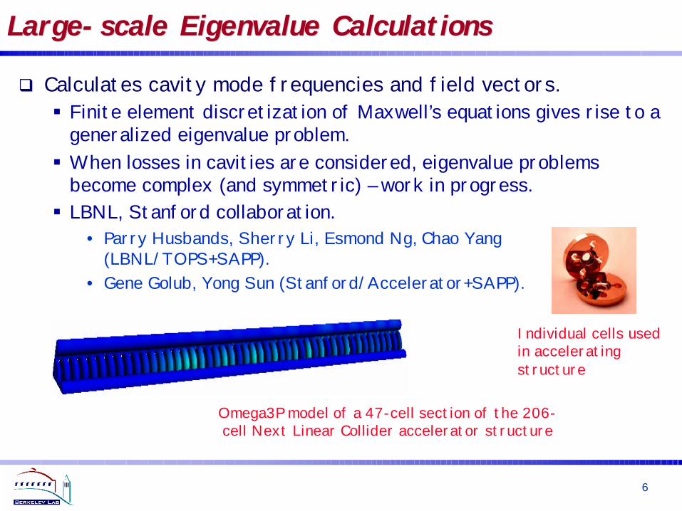
q Calculates cavity mode frequencies and field vectors.§ Finite element discretization of Maxwell’s equations gives rise to a

generalized eigenvalue problem.§ When losses in cavities are considered, eigenvalue problems

become complex (and symmetric) – work in progress.§ LBNL, Stanford collaboration.

• Parry Husbands, Sherry Li, Esmond Ng, Chao Yang (LBNL/TOPS+SAPP).

• Gene Golub, Yong Sun (Stanford/Accelerator+SAPP).

Omega3P model of a 47-cell section of the 206-cell Next Linear Collider accelerator structure

Individual cells used in accelerating structure

7

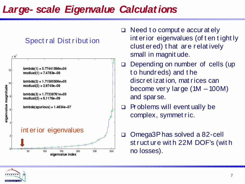
interior eigenvalues

Spectral Distribution


q Need to compute accurately interior eigenvalues (often tightly clustered) that are relatively small in magnitude.

q Depending on number of cells (up to hundreds) and the discretization, matrices can become very large (1M – 100M) and sparse.

q Problems will eventually be complex, symmetric.

q Omega3P has solved a 82-cell structure with 22M DOF’s (with no losses).

8

Two Two EigensolversEigensolvers

q Inexact shift-invert (to get an approximate solution) + Newton-type iterations (to refine the solution) – Golub, Sun (Stanford).§ Investigated and implemented different improvements for inexact shift-

invert: block algorithm, deflation techniques, and restart strategies.§ Started to investigate preconditioning techniques for the Newton-type

iterations.§ Potentially can handle very large problems.

q Exact shift-invert – Husbands, Li, Ng, Yang (LBNL).§ Require complete factorizations of (sparse) matrices.§ Make possible by exploiting work funded by TOPS – SuperLU, a high-

performance scalable parallel sparse linear equations solver.§ Combine SuperLU with PARPACK to obtain parallel implementation of

exact shift-invert Lanczos eigensolver.§ Enable accurate calculation of eigenvalues, allow verification of other

eigensolvers, and provide a baseline for comparisons.

9

TOPS Contribution TOPS Contribution -- SuperLUSuperLU

q SuperLU: direct solution of sparse linear system Ax = b.§ Efficient and portable implementations on modern computer

architectures.§ Support real and complex matrices, fill-reducing orderings,

equilibration, numerical pivoting, condition estimation, iterative refinement, and error bounds.§ New developments/improvements are funded by TOPS and

motivated by the Omega3P application.• Accommodate distributed input matrices (nearly done).

Ø Symbolic factorization still sequential but reduction in memory used.• Improve triangular solution routine (in progress).

Ø Improve management of buffers used for non-blocking operations to make it friendlier to MPI implementations.

Ø Use partial inversion to improve parallelism in the substitution process.

10


q The good news is that both the exact shift-invert and inexact shift-invert solvers produce the same eigenvalues.

q The exact shift-invert solver and inexact shift-invert solver are complementary.

q Exact-shift invert is a serious contender because of memory availability.§ Integrated as a run-time option in Omega3P.§ More comparisons using larger problems in progress.

q The exact shift-invert solver provides a quick solution to the sparse complex symmetric eigenvalue problems.

11

Future TOPS ContributionsFuture TOPS Contributions

q SuperLU:§ Improve the interface with PARPACK.§ Parallelize the remainder of the symbolic factorization routine in

SuperLU – guaranteeing memory scalability, and making the exact shift-invert algorithm much more powerful.§ Fill-reducing orderings of the matrix.

q Need to improve the Newton-type iteration for the correction step, as well as the Jacobi-Davidson algorithm:§ SuperLU has its limitations: memory bottleneck.§ Future plans include joint work (LBNL+Stanford) on the correction

step.• Iterative solvers.• Preconditioning techniques.

12

Results on NERSC SPResults on NERSC SP

48

32

p

12,477.8719,884,3874,859.8dds47 linear (16 eigenvalues)

7,430.2867,709,8514,413.9dds15 linear (14 eigenvalues)

Time(Hybrid)

Nonzeros inL+U-I

Time (ESIL)

Problem

dds47 matrix:n = 1,323,019nnz = 20,127,775

13

Adaptive Mesh Refinement in Omega3PAdaptive Mesh Refinement in Omega3P

q Adaptive mesh refinement is highly desirable to improve accuracy & optimize compute resources.

Entire 206 cell 2D Structure on 206 processors

Parallel AMR in 2D with Omega2P straightforward

Mesh level 1

Mesh level 2

RDDS 12 cell stack on 10 processorsMesh level 1 Mesh level 2

Parallel AMR in 3D with Omega3P is a challenge

14

Omega3P Optimization StrategyOmega3P Optimization Strategy

q Implement h-p adaptive refinement. q Start with coarse grid solution (h=p=E=1), devise refinement

strategy to improve accuracy in an optimal fashion.q Impose error metric used in Omega2P.

q Use RPI framework to deal with mesh partitioning and load balancing issues.

1 (Lanczos)1 (Linear)1

2 (Jacobi-Davison)2 (Quadratic)2

Eigensolverph

222H

2E

2 UdvUr

ee

µ+

ε=⋅∇=∫

15

Parallel AMR in Omega3PParallel AMR in Omega3P

q Collaborate with Y. Luo, M. Shephard (RPI/TSTT).

SolidModel

SCORECMesh Generator

InitialMesh

SCORECMesh Modification

StanfordSLAC

New Mesh

Error Information(Indicator/Estimator)

Provided by StanfordProvided by RPI SCOREC

16

CS/AM Efforts Related To Tau3PCS/AM Efforts Related To Tau3P

q Tau3P is a time domain solver for the electric and magnetic fields.

§ CAD Model/Mesh Generation.• T. Tautges (SNL) – TSTT.

§ Improvement studies for the DSI scheme.• B. Henshaw (LLNL) – TSTT.

§ Quality metrics to identify meshes with improved stability.• P. Knupp (SNL) – TSTT.• N. Folwell (SLAC) – Accelerator Project.

§ Improving parallel performance.• A. Pinar (LBNL) – TOPS; K. Devine (SNL).• A. Guetz, M. Wolf (SLAC) – Accelerator Project.

17

CAD/Meshing for PEPCAD/Meshing for PEP--II IR II IR

q Fixing CAD model and optimizing Tau3P primary/dual mesh.§ T. Tautges (SNL/TSTT).

Worst deviation= 41º

Worst deviation< .001º

18

Tau3P Stability vs. Mesh QualityTau3P Stability vs. Mesh Quality

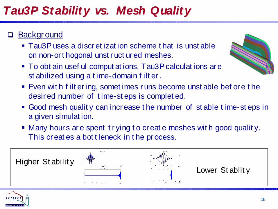
q Background§ Tau3P uses a discretization scheme that is unstable

on non-orthogonal unstructured meshes. § To obtain useful computations, Tau3P calculations are

stabilized using a time-domain filter. § Even with filtering, sometimes runs become unstable before the

desired number of time-steps is completed.§ Good mesh quality can increase the number of stable time-steps in

a given simulation.§ Many hours are spent trying to create meshes with good quality.

This creates a bottleneck in the process.

Higher StabilityLower Stablity

19


q Strategic Approach – Stabilize the Code§ B. Henshaw (LLNL/TSTT).

• The DSI (Discrete Surface Integral) scheme in Tau3P exhibits instabilities for long time integration on non-orthogonal grids that result in non-self-adjoint operator. Explored 3 possible ways to develop a stable algorithm:

1. Spatial artificial dissipation – Initial numerical experiments indicate that a sixth-order dissipation is very effective with very little damping of the energy over long times.

2. Dissipative time integration – Studied the ABS3 (Adams-BashforthStaggered-Grid Order-3) scheme but found it not suitable even though it improves the convergence properties.

3. A symmetric scheme – Developed 2nd-order and fourth-order accurate approximations that are self-adjoint but only for grids that are logically rectangular, not for general unstructured meshes. The fourth-order approximation could be used in the context of overlapping grids to give an accurate and very efficient solver.

20


q Tactical Approach: Improve Mesh Quality

§ P. Knupp (SNL/TSTT), N. Folwell (SLAC).§ It has long been observed qualitatively that the number of time-

steps one can take before going unstable depends strongly on mesh properties.§ How can we create higher quality meshes that will allow a greate

number of time steps before the onset of instability?

21


q Diagnosis of the Problem:

§ Identify specific mesh quality metrics that impact the number oftime steps allowed.§ Determine corresponding critical thresholds for the mesh quality

metrics.

22


q Empirical Approach (completed):

§ Created 25 different meshes on Pillbox § Ran the same Tau3P problem on each to get a

single number-of-time steps vs. mesh quality data point.§ Plotted number of time-steps vs. various

mesh quality metrics. (Result is a scatter plot.) § Most metrics showed low linear correlations,

but 3 were strong: Edge-length (MPES), Shape (MPCN), and Smoothness (PSM).

Strongly Correlated

Weakly Correlated

23


q Remedy (FY03):

§ Numerically optimize existing meshes via node-movement strategy (smoothing),§ Use highly correlated quality metrics (MPCN, MPES, and PSM) to

guide optimization,§ Use Mesquite (Mesh Quality Improvement) Toolkit (TSTT),§ Demonstrate that improved meshes allow larger number of time-

steps.

24

Load Balancing Issues in Tau3PLoad Balancing Issues in Tau3P

q Load balancing problem inTau3P Modeling of NLC Input Coupler.§ The use of unstructured meshes lead to matrices for

which nonzero entries are not evenly distributed.§ Makes work assignment and load balancing

difficult in a parallel setting.§ SLAC’s Tau3P currently uses ParMetis

to partition the domain to minimizecommunication – not a very satisfactory solution.

Matrix Distribution over 14 cpu’sMatrix Sparsity Parallel Speedup

25

Load Balancing Issues in Tau3PLoad Balancing Issues in Tau3P

q Collaboration between LBNL and SLAC (just started).§ Ali Pinar (LBNL/TOPS), Karen Devine (SNL).§ Adam Guetz, Michael Wolf (SLAC).

26

Visualization for Electromagnetic SystemsVisualization for Electromagnetic Systems

q G. Schussman, K. Ma (UC Davis) – SAPP.

q Extreme dense field lines.§ One hundred thousands to millions of

electron paths to visualize.§ Limited resolution of the display.§ Abstraction of the field complexity.

q User interfaces and interaction to reveal structures.

27

Interactive Visualization of Electromagnetic FieldsInteractive Visualization of Electromagnetic Fields

q Self Orienting Surface (SOS) - New representation for 3D field lines through hardware accelerated bump mapping.§ Scalable & excellent texture support.§ Fast transfer and low memory requirement.§ Perceptually correct depth cuing.

1.28(0 MB ! )

0.1240.019SOS withHardware Bump Map

1.82(628 MB ! )

0.1730.027Polygonal tubes display list

5.540.5120.077SOS, Finely tessellated (No HW Bump Map)

38.23.0010.445Polygonal tubesno display list

10k lines800 lines150 lines

SOS Performance

28

Visualizing Particles on Unstructured GridsVisualizing Particles on Unstructured Grids

q Advanced illumination and interactive methods used for displaying particles and fields simultaneously to locate regionsof interest, and multi-resolution techniques deployed to overcome performance bottlenecks.

Bunch propagation in Ptrack3D/Omega3P

29

Visualizing Dark Current SimulationVisualizing Dark Current Simulation

q Simultaneous rendering of field and particle data to study dark current generation and capture (100’s of GB).

Surface electric field magnitude, field vectors & particles

Surface electric field magnitude, & particle trajectories

30

Animation of Dynamic ProcessesAnimation of Dynamic ProcessesSimulating field and secondary emissions in a 5-cell TW-structure. Primary (green) & secondary (red) particles with surface E fields.

31

Visualization for Beam DynamicsVisualization for Beam Dynamics

q K. Ma (UC Davis) – SAPP.

q Modeling a large number of charged particles as they move through the accelerator and respond to various forces.§ Millions to billions of particles.§ Multidimensional (coordinates + momenta).§ Result in huge datasets.§ Current approaches inadequate.

(x, (x, PxPx, y) (x, , y) (x, PxPx, z) (, z) (PxPx, , PyPy, , PzPz))

32

New Hybrid Rendering AlgorithmsNew Hybrid Rendering Algorithms

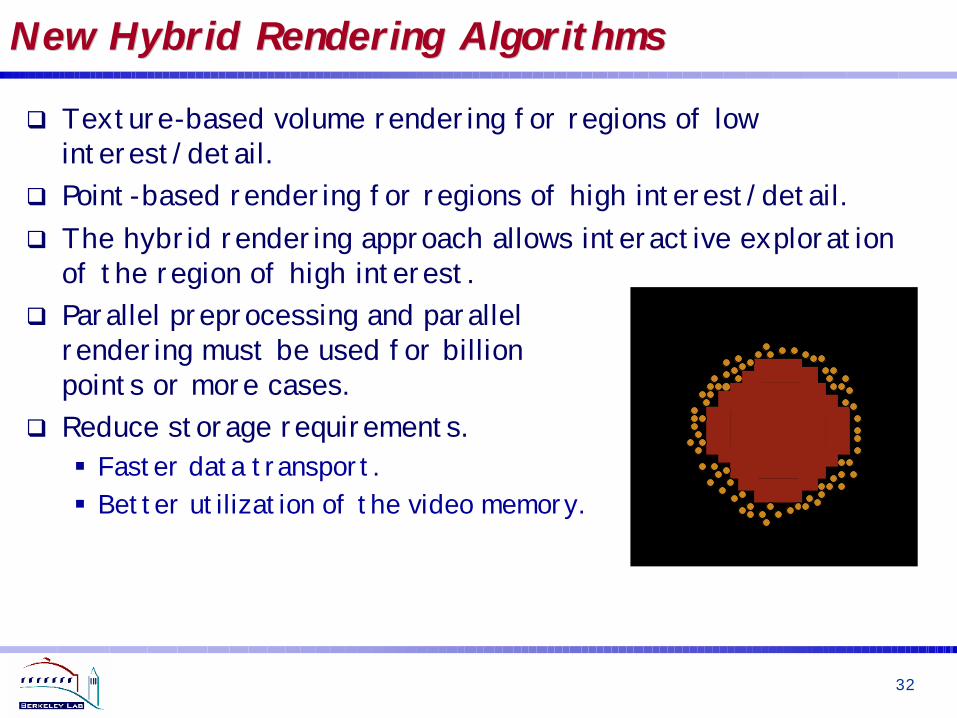
q Texture-based volume rendering for regions of low interest/detail.

q Point-based rendering for regions of high interest/detail.q The hybrid rendering approach allows interactive exploration

of the region of high interest.q Parallel preprocessing and parallel

rendering must be used for billionpoints or more cases.

q Reduce storage requirements.§ Faster data transport.§ Better utilization of the video memory.

33

CS/AM Efforts Related To Beam Dynamics CS/AM Efforts Related To Beam Dynamics

q AMR for particle-in-cell.§ Goal: Develop a flexible suite

of fast solvers for PIC codes, based on ADPEC’s Chomboframework for block-structured adaptive mesh refinement (AMR).

• Block-structured adaptive mesh solvers.

• Fast infinite-domain boundary conditions.

• Flexible specification of interaction between grid and particle data.

• Accurate representation of complex geometries.

34

AMR for PICAMR for PIC

§ Progress to date:• Developed node-centered block-structured AMR codes for Poisson’s

equation, for either rectangular domains or complex geometries.• Implemented standard PIC interpolation of charges to grid, electric

fields to particles on AMR grid.• Single-grid (non-adaptive) Chombo solution for a standard

MaryLIE/IMPACT test case produces essentially identical results.• Multiple-grid (adaptive) Chombo solution is under development.

§ Plans:• Couple Chombo AMR / PIC solver to MaryLie / IMPACT code, other

PIC codes (e.g. QuickPIC). Verification and validation, performance tuning.

• Implement fast infinite-domain boundary condition package.• Begin development of analysis-based minimum-communication solver.

35

CS/AM Efforts Related to Advanced AcceleratorsCS/AM Efforts Related to Advanced Accelerators

q Embedded boundary methods for gas jet calculations.§ Goal: Simulation of gas jets for plasma-wakefield accelerators.

• High-resolution semi-implicit finite difference approximations of time-dependent compressible viscous flows.

• Embedded boundary representation of complex geometries.• Block-structured adaptive mesh refinement.

36

AMR for Gas Jet CalculationsAMR for Gas Jet Calculations

§ Progress:• Developed grid-generation tools based on Cart3D package of

Aftosmis, Berger, and Melton.• Developed embedded-boundary AMR solver for time dependent

inviscid flows. § Plans:

• Complete development of AMR viscous solvers, semi-implicit compressible code.

• Comparisons to gas-jet experiments.• Coupling to laser energy deposition.• Develop volume-of-fluid front tracking capability to represent

boundary between jet and the vacuum more accurately.

37

Collaborations with APDECCollaborations with APDEC

q Collaborators:§ AMR / PIC :

• APDEC: Phillip Colella, Peter McCorquodale, David Serafini (LBNL). • LBNL LDRD: Alex Friedman, David Grote, Jean-Luc Vay (LBNL).• Beam Dynamics: Andreas Adelmann, Robert Ryne (LBNL).

§ Gas Jet : • APDEC: Phillip Colella, Daniel Graves, Terry Ligocki (LBNL); Anders

Petersson (LLNL); Marsha Berger (NYU).• Advanced Accelerators: Eric Esarey, Wim Leemans (LBNL).

38

Statistical MethodsStatistical Methods

q Collaborators:§ Dave Higdon, Kathy Campbell (LANL/SAPP).§ Rob Ryne (LBNL).

q Combining simulations and experimental data for forecasting, calibration, and uncertainty quantification.

q Applications: § characterizing the initial beam configuration; tuning magnetic

settings; assessing value of experimental data.q Statistical strategy/methodology includes:§ Bayesian image analysis; dimension reduction; response surface

modeling; experimental design; trading off between a few high fidelity simulations and many low fidelity simulations.

39

Using CT Data to Characterize Initial Beam ConfigurationUsing CT Data to Characterize Initial Beam Configuration

q Markov random field/wavelet prior model for initial beam.

q Conditioning on data and using many simulation runs yields a posterior distribution that describes the input beam.

q Prior information regarding the initial beam can be incorporated.

40

Supporting Computational InfrastructureSupporting Computational Infrastructure

q LBNL/NERSC§ Time allocation on IBM Power 3 SP (1M hours)§ Access to the Alvarez cluster.§ CVS§ HPSS§ Project web site§ User Services support

q ORNL§ Time allocation on IBM Power 4 SP (1.5M hours)

q Other infrastructure§ UCLA Parallel PIC Framework (Viktor Decyk)

41

Young ResearchersYoung Researchers

q LBNL …§ Parry Husbands, staff – TOPS, SAPP (eigensolvers)§ Chao Yang, staff – TOPS, SAPP (eigensolvers)§ Andreas Adelmann, postdoc – SAPP (beam dynamics)§ Laura Grigori, postdoc – TOPS (sparse matrix computation)§ Ali Pinar, postdoc – TOPS (load balancing)§ Weiguo Gao – TOPS, SAPP (eigensolvers, preconditioning)§ Keita Teranishi, graduate student – TOPS (sparse matrices)§ Summer undergraduate students – TOPS (sparse matrix tools)

q UC Davis (K. Ma) …§ Graduate tudents – SAPP (visualization)

q Stanford University (G. Golub) …§ Graduate students working – SAPP (numerical linear algebra)

applied mathematics and computer science …applied mathematics and computer science collaborations...

Documents