applied deep learning - coms0018: lab3 practical...coms0018: lab3 practical dima damen...

COMS0018: Lab3 Practical

Dima [email protected]

Bristol University, Department of Computer ScienceBristol BS8 1UB, UK

October 20, 2019


COMSM0018: Lab3 Practical Lecture - 2019/2020

Evaluation Metrics

I Let’s look again at the curves you are getting during training



Evaluation Metrics

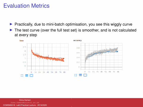
I Optimally, the loss decreases after each iteration



Evaluation Metrics

I Practically, due to mini-batch optimisation, you see this wiggly curveI The test curve (over the full test set) is smoother, and is not calculated

at every step



Evaluation Metrics - What if??

I Training Error starts to go up?!



Evaluation Metrics - What if??

I Training error wiggles A LOT?!



Hyperparameters in this practical

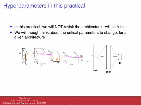
I In this practical, we will NOT revisit the architecture - will stick to itI We will though think about the critical parameters to change, for a

given architecture



Selecting hyperparameter values

I For each hyperparameters, one must understand the relationshipbetween its value and each of the following:I Training error/lossI Testing error/loss (generalisation)I Computational resources (memory and runtime)



1. Learning Rate

I The learning rate is the most important hyperparameter to set

“If you have time to tune only one parameter, tune the learning rate”1

1Goodfellow et al, p 424



1. Learning Rate

Goodfellow et al p 425



1. Learning Rate

http://cs231n.github.io/neural-networks-3/



1. Learning Rate

I You have learnt about decaying the learning rateI Remind yourself about gradient descent with momentum optimiser

from the lectures to use it in the Lab work



2. Batch-size Training

I Recall from lecture on optimisation, that there are two extremes whenperforming gradient descentI Calculating the gradient from a single exampleI Calculating the gradient for the whole dataset

I Neither is ideal, thus we typically calculate the gradient from a numberof data points

I This number is referred to as the ‘batch size’

I To correctly approximate the loss from a batch, it is crucial thatsamples are selected randomly

I However, there are approaches that sample data for a purpose (readabout hard mining)






I This number is referred to as the ‘batch size’I To correctly approximate the loss from a batch, it is crucial that

samples are selected randomly

I However, there are approaches that sample data for a purpose (readabout hard mining)






I This number is referred to as the ‘batch size’I To correctly approximate the loss from a batch, it is crucial that

samples are selected randomlyI However, there are approaches that sample data for a purpose (read

about hard mining)



2. Batch-size TrainingI The effect of changing the batch-size on the accuracy of a dataset,

depends on the datasetI The amount of wiggle in the training loss is related to the batch size.

I However there are general guidelines:I Larger batches indeed provide better approximation of the full-dataset

gradientI However, as batch size increases, the increase in accuracy or the

decrease in training time is NOT linearI Due to parallel processing, the typical limitation to batch size is the GPU

memoryI There’s a minimum size below which the gradient is too noisyI We are always searching for this sweet spot between too small and too

largeI To make the most of the GPU architectures, batches that are a power of

2 provide the best runtime - 128, 256, ...I For small-sized data samples, batches between 32 and 256 are typicalI For large-sized data samples, batches of 8 or 16 are common




depends on the datasetI The amount of wiggle in the training loss is related to the batch size.I However there are general guidelines:

I Larger batches indeed provide better approximation of the full-datasetgradient

I However, as batch size increases, the increase in accuracy or thedecrease in training time is NOT linear

I Due to parallel processing, the typical limitation to batch size is the GPUmemory

I There’s a minimum size below which the gradient is too noisyI We are always searching for this sweet spot between too small and too










I There’s a minimum size below which the gradient is too noisy

I We are always searching for this sweet spot between too small and toolarge

I To make the most of the GPU architectures, batches that are a power of2 provide the best runtime - 128, 256, ...

I For small-sized data samples, batches between 32 and 256 are typicalI For large-sized data samples, batches of 8 or 16 are common









large

I To make the most of the GPU architectures, batches that are a power of2 provide the best runtime - 128, 256, ...











2 provide the best runtime - 128, 256, ...




3. Parameter initialisation

ICML 2013




I The cost function in a DNN is non-convexI Any non-convex optimisation algorithm will depend on the initial

parameters

I In the lab you’ll use random initialisation as a practical way to initialisethe weights in a DNN

I However, more practically, it’s best to start from some pre-trainedmodel on a relevant problem with larger datasets

I In images for example, it’s customary to start from a model pre-trainedon ImageNet

I This gives an informative initial set of parameters to train CNNs whenimages are targeted





parametersI In the lab you’ll use random initialisation as a practical way to initialise

the weights in a DNN

I However, more practically, it’s best to start from some pre-trainedmodel on a relevant problem with larger datasets








the weights in a DNNI However, more practically, it’s best to start from some pre-trained

model on a relevant problem with larger datasets








the weights in a DNNI However, more practically, it’s best to start from some pre-trained

model on a relevant problem with larger datasetsI In images for example, it’s customary to start from a model pre-trained

on ImageNetI This gives an informative initial set of parameters to train CNNs when

images are targeted



4. Batch Normalisation

I Another powerful practical modification to the baseline trainingalgorithm is known as batch normalisation

I Recall the standardisation approach to data

x̂ =x − x̄σ

I The distribution of x̂ would then be zero-meaned with a standarddeviation of 1

I When training using x̂ instead of x, the training converges faster.I You can compensate for that effect on the output by learnt variables

y = λx̂ + β



4. Batch Normalisation

I When applied to each layer in the network, all layers are given thechance to converge faster

I In convolutional layers, you’ll need BatchNorm2d, while in fullyconnected layers you’ll use BatchNorm1d.

I Important: Do not add batch normalisation to your last output forclassification.

I Using batch normalisation, higher learning rates can be used.



And now....

READY....

STEADY....

GO...



applied deep learning - coms0018: lab3 practical...coms0018: lab3 practical dima damen...

Documents