applied dde, chang-yuan cheng

Introduction Delayed Negative Feedback Existence of Solutions Linear Systems and Linearization Examples and Lyapunov Fu

Applied Delayed Differential Equations

Chang-Yuan Cheng

National Pingtung University of Education

[email protected]

NCTS Summer Course on Dynamical Systems, July 17,19, 2012



Outline

1 Introduction

2 Delayed Negative Feedback

3 Existence of Solutions

4 Linear Systems and Linearization

5 Examples and Lyapunov Functions/Functionals

6 Hopf Bifurcation

Exercise :Five take-home problems. Due: Aug. 24.([email protected])



References

H. Smith, An Introduction to Delay Differential Equations withApplications to the Life Sciences, 2011

Y. Kuang, Delay Differential Equations with Applications in PopulationDynamics, Academic Press, New York, 1993.

J. Mallet-Paret and G. Sell, The Poincare-Bendixson theorem formonotone cyclic feedback systems with delay, J. Diff. Eqns. 125 (1996),441-489.

L. Shayer and S. A. Campbell, Stability, bifurcation, and multistability in asystem of two couplrd neurons with multiple time delays, SIAM AM. 61(2000), 673-700.



Examples

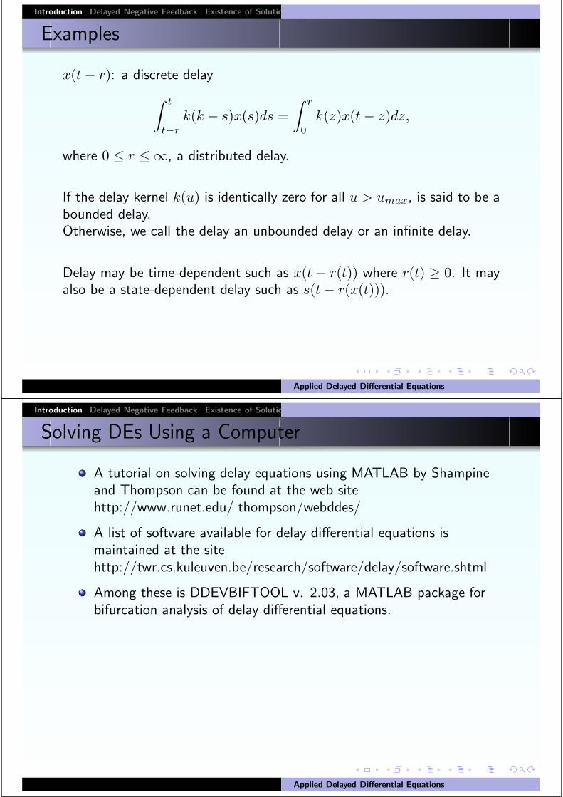
The logistic equation describing the growth of a single population

N ′(t) = N(t)[b − aN(t)].

Population density negatively affects the per capita growth rate,environmental degradation.

Hutchinson: time delay due to developmental and maturation delays.

N ′(t) = N(t)[b − aN(t − r)]

(constant delay)(discrete delay), where a, b, r > 0, r is called the delay.

Wright’s conjecture remains open.

N ′(t) = N(t)[b − a

∫ ∞

0

N(t − s)k(s)ds]

(distributed delay).Normalized,

∫ ∞

0k(s)ds = 1.



Examples

Nicholson’s blowfly equation:

N ′(t) = bN(t − r)exp(−N(t − r)

N0) − δN(t).

Blowfly eggs, larvae, sexually mature flies, for adult flies eggs take exactlyr time units to develop into adults.

The first term: accounts for recruitment of new adults, a product of afecundity term and a probability of survival from egg to adult.

The final term: death.



Examples

Busenberg and Cooke

y′(t) = b(t)y(t − T )[1 − y(t)] − cy(t).

After a delay T during which the infectious agent develops. Seasonalperiodic incidence: 0 ≤ b(t) = b(t + ω). Example:b(t) = b(1 + a sin(2πt/ω)), 0 < a < 1. c is the recovery rate.

A single self-excited neuron with delayed excitation:

x′(t) = −αx(t) + tanh(x(t − τ)).

x(t) encodes the neuron’s activity level. The delay τ represents thetransmission time between output x(t) and input.

y′i(t) = −Aiyi(t) +

n∑j=1

Wijtanh(yj(t − τij)) + Ii(t).

τij is the delay in signal transmission between the jth neuron and ithneuron.

W i d R h th t ill ti f th tApplied Delayed Differential Equations


Examples

x(t − r): a discrete delay

∫ t

t−r

k(k − s)x(s)ds =

∫ r

0

k(z)x(t − z)dz,

where 0 ≤ r ≤ ∞, a distributed delay.

If the delay kernel k(u) is identically zero for all u > umax, is said to be abounded delay.Otherwise, we call the delay an unbounded delay or an infinite delay.

Delay may be time-dependent such as x(t − r(t)) where r(t) ≥ 0. It mayalso be a state-dependent delay such as s(t − r(x(t))).



Solving DEs Using a Computer

A tutorial on solving delay equations using MATLAB by Shampineand Thompson can be found at the web sitehttp://www.runet.edu/ thompson/webddes/

A list of software available for delay differential equations ismaintained at the sitehttp://twr.cs.kuleuven.be/research/software/delay/software.shtml

Among these is DDEVBIFTOOL v. 2.03, a MATLAB package forbifurcation analysis of delay differential equations.



Preliminaries

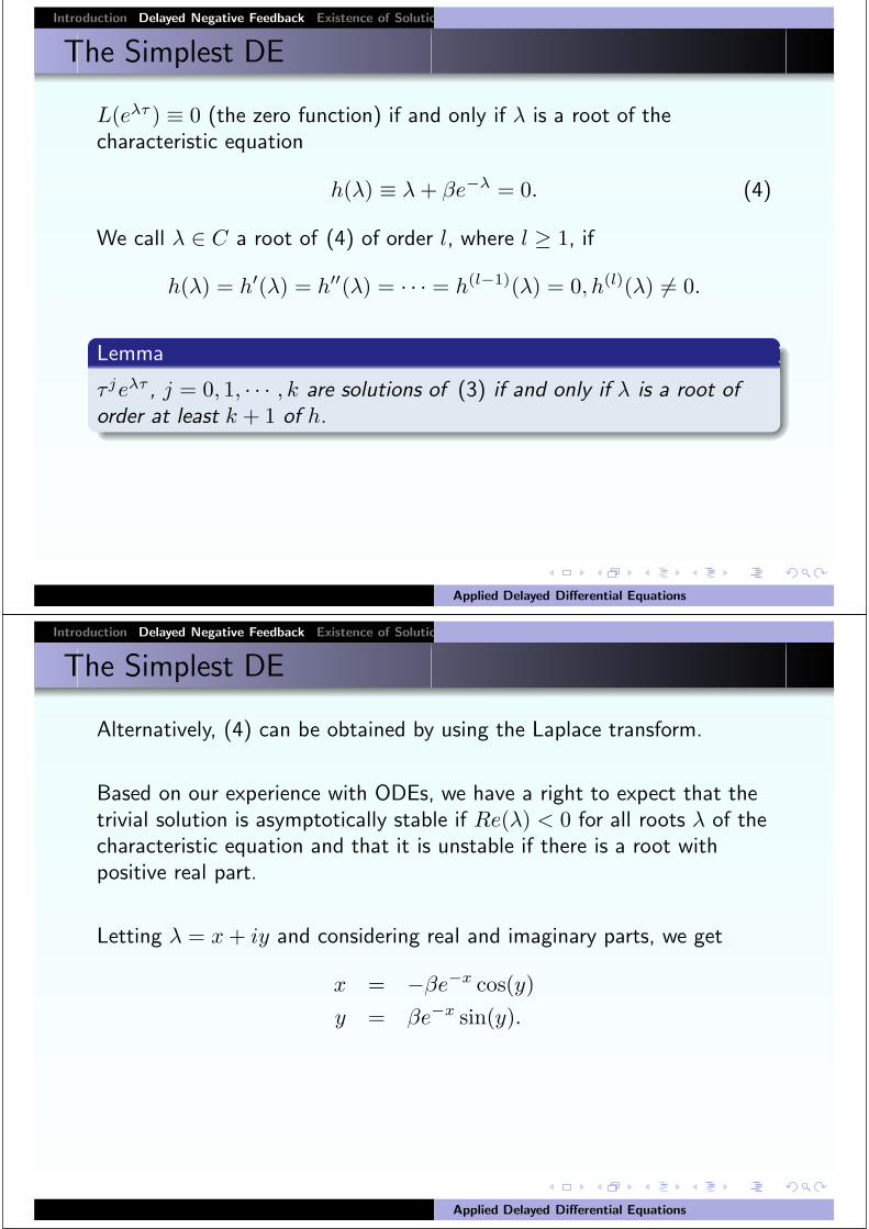
u′(t) = −u(t − τ). (1)

The method of steps.By using the MATLAB DDE23 package.Fig.: Solution of equation (1) with initial data u(θ) = 1, θ ∈ [−1, 0], forvarious τ .

τ = 0.25-no oscillations

τ = 0.6-hint of oscillations

τ = 1.0-damped oscillations

τ = 1.5-barely damped oscillations

τ = 2.0-undamped oscillations

u ≡ 0 is a solution, a steady-state solution. It is stable when τ < π/2and unstable when τ > π/2 ≈ 1.58.



The Simplest DE

u′(t) = −αu(t − r), (2)

r ≥ 0. The case α > 0 is of most interest inasmuch as it corresponds tonegative feedback; α > 0 is the positive feedback case. When r = 0,u = 0 is an asymptotically stable steady state for the case of negativefeedback; it is unstable for positive feedback. What happens when r > 0?U(τ) = u(t). τ = t

r . β = αr.

dU

dτ= −βU(τ − 1). (3)

We seek (complex) values of λ such that U(τ) = exp(λτ) is a solution of(3). It is convenient to introduce the linear operator, defined on thedifferentiable functions, by

L(U) =dU

dτ+ βU(τ − 1).

ThenL(eλτ ) = λeλτ + βeλ(τ−1) = eλτ [λ + βe−λ].



The Simplest DE

L(eλτ ) ≡ 0 (the zero function) if and only if λ is a root of thecharacteristic equation

h(λ) ≡ λ + βe−λ = 0. (4)

We call λ ∈ C a root of (4) of order l, where l ≥ 1, if

h(λ) = h′(λ) = h′′(λ) = · · · = h(l−1)(λ) = 0, h(l)(λ) �= 0.

Lemma

τ jeλτ , j = 0, 1, · · · , k are solutions of (3) if and only if λ is a root oforder at least k + 1 of h.



The Simplest DE

Alternatively, (4) can be obtained by using the Laplace transform.

Based on our experience with ODEs, we have a right to expect that thetrivial solution is asymptotically stable if Re(λ) < 0 for all roots λ of thecharacteristic equation and that it is unstable if there is a root withpositive real part.

Letting λ = x + iy and considering real and imaginary parts, we get

x = −βe−x cos(y)

y = βe−x sin(y).



The Simplest DE

Lemma

The following hold.

If β < 0, then there is exactly one real root and it is positive.

If 0 < β < e−1, then there are exactly two real roots x1 < x2, bothnegative. x1 → −∞ and x2 → 0 as β → 0.

If β = e−1, then there is a single real root of order two, namelyλ = −1

If β > e−1, then there are no real roots.



The Simplest DE

Proposition

The following hold for (4).

1. If 0 < β < π/2, then there exists δ > 0 such that R(λ) ≤ −δ forall roots.

2. If β = π/2, then λ = ±iπ/2 are roots of order one.

3. If β > π/2, there are roots λ = x ± iy with x > 0, y ∈ (π/2, π).

Corollary

The following hold for (2).

If α < 0, then u = 0 is unstable.

If 0 < rα < π/2, u = 0 is asymptotically stable.

If rα = π/2, u = sin(πτ/2), cos(πτ/2) are solutions.

If rα > π/2, u = 0 is unstable.



The Simplest DE

Figure: The stability region in the (r, α)-plane for (2).

Simulation: Simulation of (2) for α = 1, r = 1.4 and 1.58, I.C. = 1.



Oscillation of Solutions

Theorem

For every real α and r > 0 the following are equivalent.

Every solution of (2) is oscillatory.

rα > 1/e.



The Method of Steps

Existence and uniqueness of solutions of discrete-delay differentialequations is established by the method of steps, appealing to classicalODE results.More general delay equations require a more general framework forexistence and uniqueness.

Solutions either extend to the entire half-line or blowup in finite time.Applications to biology require that solutions that start positive, staypositive in the future.Differential inequalities involving delays are important tools with which tobound solutions.

x′(t) = f(t, x(t), x(t − r)) (5)

x(t) = φ(t), s − r ≤ t ≤ s (6)



The Method of Steps

Theorem

Let f(t, x, y) and fx(t, x, y) be continuous on R3, s ∈ R, and let

φ : [s − r, s] → R be continuous. Then there exist σ > s and a uniquesolution of the initial-value problem (5) on [s − r, σ].

The previous theorem provides only a local solution of (5). Just as forODEs, we can often, but not always, extend this solution to be definedfor all t ≥ s.

Theorem

Let f satisfy the hypotheses of The previous theorem and letx : [s − r, σ) → R be the noncontinuable solution of the initial-valueproblem (5). If σ < ∞ then

limt→σ− |x(t)| = ∞



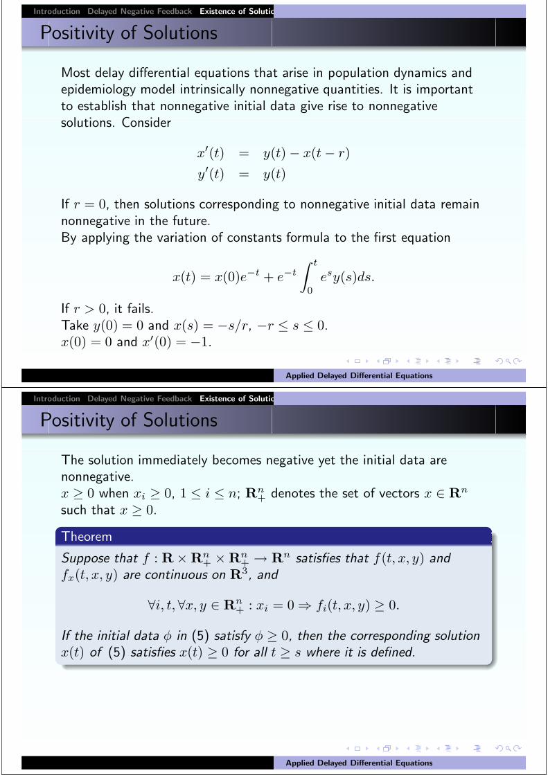
Positivity of Solutions

Most delay differential equations that arise in population dynamics andepidemiology model intrinsically nonnegative quantities. It is importantto establish that nonnegative initial data give rise to nonnegativesolutions. Consider

x′(t) = y(t) − x(t − r)

y′(t) = y(t)

If r = 0, then solutions corresponding to nonnegative initial data remainnonnegative in the future.By applying the variation of constants formula to the first equation

x(t) = x(0)e−t + e−t

∫ t

0

esy(s)ds.

If r > 0, it fails.Take y(0) = 0 and x(s) = −s/r, −r ≤ s ≤ 0.x(0) = 0 and x′(0) = −1.




The solution immediately becomes negative yet the initial data arenonnegative.x ≥ 0 when xi ≥ 0, 1 ≤ i ≤ n; R

n+ denotes the set of vectors x ∈ R

n

such that x ≥ 0.

Theorem

Suppose that f : R × Rn+ × R

n+ → R

n satisfies that f(t, x, y) andfx(t, x, y) are continuous on R

3, and

∀i, t,∀x, y ∈ Rn+ : xi = 0 ⇒ fi(t, x, y) ≥ 0.

If the initial data φ in (5) satisfy φ ≥ 0, then the corresponding solutionx(t) of (5) satisfies x(t) ≥ 0 for all t ≥ s where it is defined.




Example: the discrete-delay predator-prey model

N ′1(t) = N1(t)[b − N2(t)] (7)

N ′2(t) = N2(t)[−c + N1(t − r)],

where b,c > 0 and delay r > 0 reflects a delay in assimilation ofconsumed prey. Nonnegative initial conditions:

N1(t) = φ1(t),−r ≤ t ≤ 0 (8)

N2(0) = N02 .

x = (x1, x2) where xi = Ni(t), y = (y1, y2) where yi = Ni(t − r)

f(t, x, y) = (x1[b − x2], x2[−c + y1])

f ,fx exist and are continuous so it has a unique noncontinuable solutiondefined on some interval [−r, σ) where σ > 0.This solution has nonnegative components.If x,y ≥ 0 and xi = 0 for some i, then fi(t, x, y) = 0, σ = +∞.



Stability Definitions

Considerx′(t) = f(t, xt).

Suppose f(t, 0) = 0, t ∈ R.The solution x = 0 is stable if for any σ ∈ R and ε > 0, there existsδ = δ(σ, ε) > 0 such that φ ∈ C and ‖φ‖ < δ implies that‖xt(σ, φ)‖ < ε, t ≥ σ.

It is asymptotically stable if it is stable and if there exists b(σ) > 0 suchthat whenever φ ∈ C and ‖φ‖ < b(σ), then x(t, σ, φ) → 0, t → ∞.

x = 0 is unstable if it is not stable.

The stability of any other solution can be defined by changing variablessuch that the given solution is the zero solution.



Exercise

Exercise 1: Aiello and Freedman introduce a model of a stage-structuredpopulation consisting of immature x1 and mature x2 individuals:

x′1(t) = rx2(t) − dx1(t) − βe−dτx2(t − τ)

x′2(t) = βe−dτx2(t − τ) − ax2

2(t).

Do nonnegative initial data give rise to nonnegative solution?



Automous Linear Systems

Although the method is similar to that for ODEs, the characteristicequation is more complicated, typically having infinitely many roots.Fortunately, all but finitely many of these roots have real part less thanany given real number.In this chapter, C = C([−r, 0],Cn).A function L:C → C

n is linear if

L(aφ + bψ) = aL(φ) + bL(ψ), φ, ψ ∈ C, a, b ∈ C.

L is said to be bounded if there exists K > 0 such that

|L(φ)| ≤ K‖φ‖, φ ∈ C

x′(t) = L(xt) (9)

Let A and B be n × n matrices and define

L(φ) = Aφ(0) + Bφ(−r).

Then|L(φ)| ≤ |A||φ(0)| + |B||φ(−r)| ≤ (|A| + |B|)‖φ‖

L is bounded.Applied Delayed Differential Equations


Automous Linear Systems

x′(t) = Ax(t) + Bx(t − r)

x′(t) = Ax(t) +

m∑j=1

Bjx(t − rj)

Assume that ri,j > 0, i, j = 1, 2. kij : [0, rij ] → C.

x′1(t) =

∫ r11

0

k11(s)x1(t − s)ds +

∫ r12

0

k12(s)x2(t − s)ds (10)

x′2(t) =

∫ r21

0

k21(s)x1(t − s)ds +

∫ r22

0

k22(s)x2(t − s)ds

Let r = max rij and extend kij to [0,r] if necessary by making itidentically zero on (rij ,r]. k(s) = (kij(s)), x(t) = (x1(t), x2(t)).Then

x′(t) =

∫ r

0

k(s)x(t − s)ds



Laplace Transform and Variation of Constants Formula

x′(t) = Ax(t) + Bx(t − r) + f(t), t ≥ 0, x0 = φ, (11)

where A, B are scalars; the case that they are matrices is treated byanalogy.The Laplace transform:

F (s) = L(f) =

∫ ∞

0

e−stf(t)dt,

where f : [0,∞) → C is an exponentially bounded function,|f(t)| ≤ Mekt for some real M , k.If f , g:[0,∞) → C then their convolution is defined by

(f ∗ g)(t) =

∫ t

0

f(τ)g(t − r)dτ =

∫ t

0

f(t − τ)g(τ)dτ

ThenL(f ∗ g) = F (s)G(s),

where F = L(f) and G = L(g).




Applying the transform to (11)

sX(s) − φ(0) = AX(s) + B[

∫ r

0

e−stφ(t − r)dt +

∫ ∞

r

e−stx(t − r)dt] + F (s

= AX(s) + B[

∫ r

0

e−stφ(t − r)dt + e−srX(s)] + F (s)

= [A + e−srB]X + B

∫ r

0

e−stφ(t − r)dt + F (s)

= [A + e−srB]X + BΦ(s) + F (s), (12

Φ = L(φ(· − r)) and extending φ to [−r,∞) by making it zero for t > 0.

X(s) = K(s)[φ(0) + BΦ(s) + F (s)]

whereK(s) = (s − A − e−srB)−1

k: the inverse transform of K. k is the solution of (11), with f=0, forthe initial data

ξ(θ) =

{1, θ = 00, −r ≤ θ < 0.




In fact, k(t) = eAt, 0 ≤ t < r, and it satisfies the initial value problem:

x′(t) = Ax(t) + BeA(t−r), x(r) = eAr, r ≤ t < 2r.

k is called the fundamental solution of (11).

x(t) = x(t; φ, f) = x(t; φ, 0) + x(t; 0, f)

x(t; 0, f) =

∫ t

0

k(t − τ)f(τ)dτ

x(t; φ, 0) = k(t)φ(0) +

∫ t

0

k(t − τ)Bφ(τ − r)dτ

These formulas hold with minor changes in the case that (11) is a vectorsystem with matrices A, B.



The Characteristic Eq.

We seek exponentially growing solutions of (9),

x(t) = eλtv, v �= 0.

λ is complex, v is a vector whose components are complex on [−r, 0],expλ(θ) = eλθ.

xt(θ) = x(t + θ) = eλ(t+θ)v = eλtexpλ(θ)v

x′(t) = λeλtv = L(xt) = eλtL(expλv)

λv = L(expλv)

Writing v =∑

j vjej where {ej}j is the standard basis for Cn, then

L(expλv) =∑

j vjL(expλej).




Define the n × n matrix

Lλ = (L(expλe1)|L(expλe2)| · · · |L(expλen)) = (Li(expλej)),

where Li(φ) is component i of L(φ).Then L(expλv) = Lλv and x(t) = eλtv is a nonzero solution of (9) if λis a solution of the characteristic eqution:

det(λI − Lλ) = 0.

Lemma

h(λ) = det(λI − Lλ) is an entire function.

Properties of nontrivial entire functions, in particular of h, are:

Each characteristic root has finite order.

There are at most countably many characteristic roots.

The set of characteristic roots has no finite accumulation point.

Remarkably, there are only finitely many characteristic roots with positivereal part.




Lemma

Given σ ∈ R, there are at most finitely many characteristic rootssatisfying Re(λ) > σ. If there are infinitely many distinct characteristicroots {λn}n, then

Re(λn) → −∞, n → ∞

An important implication of the previous lemma is that there existsσ ∈ R and a finite set of “dominant characteristic roots” having maximalreal part equal to σ with all other roots having real part strictly less thanσ.

Proposition

Suppose that L maps real functions to real vectors:L(C([−r, 0],Rn)) ⊂ R

n. Then λ is a characteristic root if and only if λis a characteristic root.




Theorem

Suppose that Re(λ) < µ for every characteristic root λ. Then thereexists K > 0 such that

|x(t, φ)| ≤ Keµt‖φ‖, t ≥ 0, φ ∈ C

where x(t, φ) is the solution of (9) satisfying x0 = φ. In particular,x = 0 is asymptotically stable for (9) if Re(λ) < 0 for everycharacteristic root; it is unstable if there is a root satisfying Re(λ) > 0.



Small Delays Are Harmless

The linear delay system

z′(t) = Az(t) + Bz(t − r)

Nondelayed counterpart

z′(t) = (A + B)z(t)

the characteristic equation:

h(λ, r) = det[λI − A − e−λrB] = 0 (13)

h(λ, 0) = det[λI − A − B] = 0

Theorem

Let z1, z2, · · · , zk be the distinct eigenvalues of A + B, let δ > 0, and lets ∈ R satisfy s < miniRe(zi). Then there exists r0 > 0 such that if0 < r < r0 and h(z, r) = 0 for some z then either Re(z) < s or|z − zi| < δ for some i.



Small Delays Are Harmless

In words, for small enough delay, the characteristic roots of (13) areeither very near the eigenvalues of A + B or have more negative realparts than any of the eigenvalues of A + B.Small delays are harmless in the sense that if asymptotic stability holdswhen τ = 0, then it continues to hold for small delays in as much as wemay choose δ small enough that the δ-ball about each eigenvalue ofA + B belongs to the left half-plane and we may choose s negative.



The Scalar Equation

A and B are real scalars.

x′(t) = Ax(t) + Bx(t − r) (14)

λ = A + Be−λr

z = rλ, α = Ar, β = Br

z = α + βe−z. (15)

If we write z = x + iy, then

0 = x − α − βe−x cos(y)

0 = y + βe−x sin(y)

z = 0 is a root precisely when α + β = 0.



The Scalar Equation

Define F (z, α, β) := z − α − βe−z.Setting x = 0 and solving for α and β gives the “neutral stability curves”in parameter space

α = y cos(y)/ sin(y)

β = −y/ sin(y)

We denote by

C0 := {(α, β) = (y cos(y)/ sin(y),−y/ sin(y)), 0 ≤ y < π}The curve along which z = ±iy, 0 ≤ y < ± are roots.

dα

dy< 0,

dβ

dy< 0, 0 < y < π

Searting from (1,−1) when y = 0, meets the β-axis at (0,−π/2) wheny = π/2.Approaches (−∞,−∞) from below and tangent to the line α = β asy ↗ π because α/β = − cos(y) → 1 whereas both α, β → −∞ asy ↗ π.



The Scalar Equation

We also consider the curves

Cn := {(α, β) = (y cos(y)/ sin(y),−y/ sin(y)), nπ < y < (n+1)π}, n ≥ 1,

where z = ±iy, nπ < y < (n + 1)π are roots.On Cn, dα/dy < 0 but dβ/dy changes sign on (nπ, (n + 1)π) wheretan(y) = y. |β/α| > 1 on Cn implying that C1, C3, · · · lie strictly abovethe graph of β = |α| and C2, C4, · · · lie strictly below the graph ofβ = −|α|.

Figure: Stability region for (15) in the (α, β)-plane lies to the left of thedisplayed curve. Applied Delayed Differential Equations


The Scalar Equation

We assume that A + B �= 0 for otherwise λ = 0 is a root.

Theorem

The following hold for (14)G

If A + B > 0, then x = 0 is unstable.

If A + B < 0 and B ≥ A, then x = 0 is asymptotically stable.

If A + B < 0 and B < A, then there exists r∗ > 0 such that x = 0is asympototically stable for 0 < r < r∗ and unstable for r > r∗.

In case (c), there exist a pair of purely imaginary roots at

r = r∗ =cos−1(−A/B)√

B2 − A2.



Linearized Stability

Consider the nonlinear functional differential equation

x′(t) = f(xt). (16)

Then x(t) = x0 ∈ Rn, r ∈ R is a steady-state solution of (16) if and

only iff(x0) = 0

where x0 ∈ C is the constant function equal to x0.If x(t) is a solution of (16) and

x(t) = x0 + y(t)

theny′(t) = f(x0 + yt).

To understand the behavior of solutions of y′(t) = f(x0 + yt) forsolutions that start near y = 0.




Assume thatf(x0 + φ) = L(φ) + g(φ), φ ∈ C,

where L : C → Rn is a bounded linear function and g : C → R

n is“higher order” in the sense that

limφ→0

|g(φ)|‖φ‖ = 0.

The linear systemz′(t) = L(zt)

is called the linearized (or variational) equation about the equilibrium x0.We must view it on the complex space C = C([−r, 0],Cn).




Theorem

Let ∆(λ) = 0 denote the characteristic equation corresponding toz′(t) = L(zt) and suppose that

−σ := max�(λ)=0

Re(λ) < 0.

Then x0 is a locally asymptotically stable steady state of (16). In fact,there exists b > 0 such that

‖φ − x0‖ < b ⇒ ‖xt(φ) − x0‖ ≤ K‖φ − x0‖e−σt/2, t ≥ 0.

If Re(λ) > 0 for some characteristic root, then x0 is unstable.




Considerx′(t) = F (x(t), x(t − r))

where F : D × D → Rn is continuously differentiable and D ⊂ R

n isopen. If F (x0, x0) = 0 for some x0 ∈ D, then x(t) = x0, t ∈ R is anequilibrium solution. Then f(φ) = F (φ(0), φ(−r)) so

f(x0 + φ) = Aφ(0) + Bφ(−r) + G(φ(0), φ(−r))

where A = fx(x0, x0), B = fy(x0, x0).It follows that the linearized system about x = x0 is

x′(t) = Ax(t) + Bx(t − r)

Consider the scaled version of the delayed chemostat model

S′(t) = 1 − S(t) − f(S(t))x(t) (17)

x′(t) = e−rf(S(t − r))x(t − r) − x(t),

where f(S) = mS/(a + S) and x, S ≥ 0.




Nonnegative equilibria consist of the “washout state” (S, x) = (1, 0) and,if f(1) > er, the “survival state” (S, x) = (S, x), where f(S) = er andx = (1 − S)e−r.

A =

( −1 − xf ′(S) −f(S)0 −1

), B = e−r

(0 0

f ′(S)x f(S)

)

(λ + 1)(λ + 1 + xf ′(S) − e−rf(S)e−λr) = 0

What luck that if factors! λ = −1, and

λ = −1 − xf ′(S) + e−rf(S)e−λr

For the washout state, a = −1 and b = e−rf(1). Hence,a + b = −1 + e−rf(1) and b > a.The washout state is asymptotically stable when e−rf(1) < 1 butunstable if e−rf(1) > 1, when the survival state exists.




For the survival state, a = −1 − xf ′(S) and b = 1, so a + b < 0 andb > a. Therefore, the survival state is asymptotically stable when it exists.

Exercise 2: Show that z = 0 is a double root of z = α + βe−z only whenα = 1 and β = −1. In fact, the only double roots are at z = α − 1 whenα = 1 + log |β|, β < 0. There are no roots of order three or higher.

Exercise 3: Consider the Lotka-Volterra competition system

x′(t) = x(t)[2 − ax(t) − by(t − r)]

y′(t) = y(t)[2 − cx(t − r) − dy(t)]

Determine the stability of the positive steady state when a = d = 2and b = c = 1. How does it depend on r?

Determine the stability of the positive steady state when a = d = 1and b = c = 2. How does it depend on r?



Delayed Logistic Equation

[Hutchinson, 1948], the delayed logistic equation

n′(t) = a[1 − n(t − T )/K]n(t).

Let N(t) = n(t)/K and rescale time, then

N ′(t) = N(t)[1 − N(t − r)], t ≥ 0. (18)

We are primarily interested in nonnegative solutions.

Proposition

Every orbit of (18) with φ ≥ 0 is bounded. In fact, for each such φ,there exists T > 0 such that

0 ≤ N(t, φ) ≤ er, r > T




Putting u = N − 1, it becomes the famous Wright’s equation

u′(t) = −u(t − r)[1 + u(t)]

The steady-state N = 1 is now u = 0, the linear equation

v′(t) = −v(t − r)

will determine the stability of our N = 1 steady state. Recall that ifr < π/2 then v = 0 is asymptotically stable and if r > π/2, then v = 0 isunstable. Wright proved the following.

Theorem

(see [Kuang, 1993]) If r ≤ 3/2, then N(t, φ) → 1, t → ∞ for allsolutions of (18) satisfying φ(0) > 0.

Note that 3/2 = 1.5 < 1.57 · · · = π/2. Wright’s conjecture, stillunsolved, is that the previous theorem holds with π/2 instead of 3/2.




Simulations: Simulations of (18) for different values of r(r = 0.25, 1.52, 1.60); N0 = 0.5.



Liapunov Functions

Considerx′(t) = f(xt),

where f : C → Rn is locally Lipschitz and completely continuous.Let x(t) = x(t, φ) be the solution satisfying x0 = φ.Given V : C → R, define

V (φ) = limh↘0+

1

h[V (xh(φ)) − V (φ)]

if the limit exists.

Theorem

(The LaSalle invariance principle) If V is a Liapunov function on G andxt(φ) is a bounded solution such that xt(φ) ∈ G, t ≥ 0, then ω(φ) �= 0 iscontained in the maximal invariant subset of S ≡ ψ ∈ G : V (ψ) = 0.



Logistic Eq., Instantaneous/Delayed Density Dependence

Considerx′(t) = rx(t)[1 − a1x(t) − a2x(t − τ)]. (19)

We rewrite it as

x′(t) = rx(t)[−a1(x(t) − x∗) − a2(x(t − τ) − x∗)]

Let G = {φ ∈ C : φ ≥ 0, φ(0) > 0} and define V : G → R by

V (φ) = φ(0) − x∗ − x∗ log(φ(0)/x∗) + η

∫ 0

−τ

(φ(s) − x∗)2ds

where η > 0 is to be determined.Exercise 4: Verify that V (φ) satisfies:

V is continuous on G and becomes infinite at a boundary pointwhere φ(0) = 0,

it is positive definite with respect to X∗ ∈ C, the functionidentically equal to x∗, in the sense that

V (φ) > 0 = V (X∗), φ ∈ G, φ �= X∗.




If x(t, φ) is a solution of (19) with φ ∈ G, then xt(φ) ∈ G for t ≥ 0 and

V (xt) = x(t) − x∗ − x∗ log(x(t)/x∗) + η

∫ 0

−τ

(x(t + s) − x∗)2ds

= x(t) − x∗ − x∗ log(x(t)/x∗) + η

∫ t

t−τ

(x(s) − x∗)2ds (20)

d

dtV (xt) =

x(t) − x∗

x(t)x′(t) + η[(x(t) − x∗)2 − (x(t − τ) − x∗)2]

=x(t) − x∗

x(t)rx(t)[−a1(x(t) − x∗) − a2(x(t − τ) − x∗)]

+η[(x(t) − x∗)2 − (x(t − τ) − x∗)2]

= −ra1(x(t) − x∗)2 − ra2(x(t) − x∗)(x(t − τ) − x∗)

+η[(x(t) − x∗)2 − (x(t − τ) − x∗)2]

= −(ra1 − η)(x(t) − x∗)2 − ra2(x(t) − x∗)(x(t − τ) − x∗)

−η(x(t − τ) − x∗)2




If we take η = ra1/2, then

d

dtV (xt) = −(ra1/2)(x(t) − x∗)2 − ra2(x(t) − x∗)(x(t − τ) − x∗)

−(ra1/2)(x(t − τ) − x∗)2

= W (x(t) − x∗, x(t − τ) − x∗) (21)

where

W (u, v) = −(ra1/2)u2 − ra2uv − (ra1/2)v2

= − r

2

(a1 a2

a2 a1

) (uv

)·(

uv

)(22)

The symmetric matrix has eigenvalues a1 ± a2, both positive if a1 > a2,and therefore

d

dtV (xt) = W (x(t) − x∗, x(t − τ) − x∗) ≤ 0, t ≥ 0, φ ∈ G




Theorem

If a1 > a2 and φ ∈ G, then ω(φ) = X∗ and x(t, φ) → x∗ as t → ∞.

Exercise 5: Cooke modeled a vector borne disease by

y′(t) = by(t − r)[1 − y(t)] − cy(t)

where b, r > 0 and c ≥ 0. y(t) denotes the fraction of human populationthat is infected with the disease, c is the recovery rate, r is the delaybetween when a vector (e.g., a mosquito) becomes infected after bitingan infected person until the time when its bite can infect a human, and bis the contact rate. Show that G = {φ ∈ C : 0 ≤ φ(θ) ≤ 1} is positivelyinvariant as the model demands. If c > b > 0, show that the trivialsolution is globally attracting. Hint: the Lyapunov function

V (φ) =1

2cφ(0)2 +

1

2

∫ 0

−r

φ2(θ)dθ.

PS: You may also use the monotone dynamics.



A Canonical Example

Considerx′(t) = x(t − 1)[−v + x2(t) + x2(t − 1)], (23)

where v is a real parameter. 0 is a steady state for all v, ±√

v/2 is asteady state for v > 0. Focus on the steady-state x = 0 first. Linearizingabout x = 0, we get

y′(t) = −vy(t − 1)

Its characteristic equation is

λ = −ve−λ

y = 0 is asymptotically stable for 0 < v < π/2. At v = 0, λ = 0 is theonly root. At v = π/2, λ = ±iπ/2 are roots. Therefore x = 0 isasymptotically stable for (23) when 0 < v < π/2.



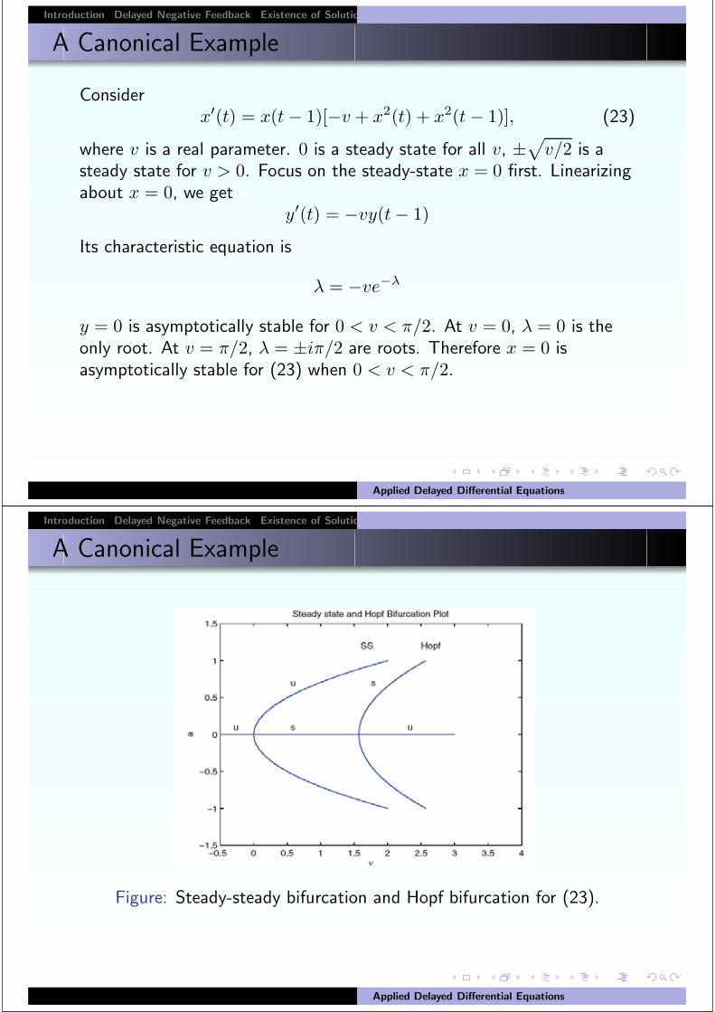
A Canonical Example

Figure: Steady-steady bifurcation and Hopf bifurcation for (23).



A Canonical Example

At v = π/2, y(t) = sin(πt/2), y(t) = cos(πt/2). Try

x(t) = a sin(πt/2)

aπ

2= av − a3

x(t) = ±√

v − π

2· sin(πt/2), v >

π

2

is a periodic solution of (23).



Hopf Bifurcation Theorem

x′(t) = F (xt, µ) (24)

F : C × R → Rn is twice continuously differentiable

F (0, µ) ≡ 0.

F (φ, µ) = L(µ)φ + f(φ, µ)

limφ→0

|f(φ, µ)|‖φ‖ = 0

The characteristic equation

0 = det(λI − A(µ, λ)), Aij(µ) ≡ L(µ)i(eλej)

(H) For µ = 0, the characteristic equation has a pair of simple roots±iω0 with ω0 �= 0 and no other root that is an integer multiple of iω0.




If we express the characteristic equation as h(µ, λ) = 0, then (H) impliesthat the partial derivative hλ(0, iω0) �= 0. λ = λ(µ) = α(µ) + iω(µ) forsmall µ satisfying λ(0) = iω0. In particular, α(0) = 0 and ω(0) = ω0.

Theorem

Let (H) and α′(0) > 0 hold. Then there exists ε0 > 0, real-valued evenfunctions µ(ε) and T (ε) > 0 satisfying µ(0) = 0 and T (0) = 2π/ω0, anda nonconstant T (ε)-periodic function p(t, ε), with all functions beingcontinuously differentiable in ε for |ε| < ε0, such that p(t, ε) is a solutionof (24) and p(t, ε) = εq(t, ε) where q(t, 0) is a 2π/ω0-periodic solutionof q′ = L(0)q.Moreover, there exist µ0,β0,δ > 0 such that if (24) has a nonconstantperiodic solution x(t) of period P for some µ satisfying |µ| < µ0 withmaxt |x(t)| < β0 and |P − 2π/ω0| < δ, then µ = µ(ε) andx(t) = p(t + θ, ε) for some |ε| < ε0 and some θ.




Theorem

(Conti.) If F is five times continuously differentiable then:

µ(ε) = µ1ε2 + O(ε4)

T (ε) =2π

ω0[1 + τ1ε

2 + O(ε4)]

If all other characteristic roots for µ = 0 have strictly negative real partsexcept for ±iω0 then p(t, ε) is asymptotically stable if µ1 > 0 andunstable if µ1 < 0.

µ1 > 0:“supercritical” Hopf bifurcation. µ1 < 0: “subcritical” Hopfbifurcation.



Delayed Negative Feedback

Considerx′(t) = −f(x(t − r))

f(0) = 0, f ′(0) = 1, f ′′(0) = A, f ′′′(0) = B

The equation exhibits negative feedback in view of the negative sign andin the sense that xf(x) > 0, at least for x near zero. In the absence ofthe delay, x = 0 would be an asymptotically stable equilibrium. Bys = t/r.

x(s) = −rf(x(s − 1))

The linearized equation about x = 0 is

v(s) = −rv(s − 1)

with the characteristic equation

λ + re−λ = 0

The roots have negative real part when 0 ≤ r < π/2; λ = ±iπ/2 areroots at r = π/2 and all other roots have negative real part.




Set r = π/2 + µ

F (λ, µ) ≡ λ + (π/2 + µ)e−λ = 0. (25)

F (iπ/2, 0) = 0, Fλ(iπ/2, 0) = 1 + (π/2)i, Fµ(iπ/2, 0) = −i.

the implicit function theorem implies that we can solve F = 0 forλ = λ(µ) = α(µ) + iω(µ) satisfying λ(0) = (π/2)i and

dλ

dµ(0) = −Fµ/Fλ =

π/2 + i

1 + (π/2)2

Consequently,dα

dµ(0) =

π/2

1 + (π/2)2




When µ = 0 there exists δ > 0 such that the roots of the characteristicequation consist of ±i(π/2) and roots λ satisfying Re(λ) < −δ.

By the continuity of the roots with respect to µ, there exists µ0 > 0 suchthat for |µ| < µ0, the roots of (25) consist of α(µ) ± iω(µ) and otherroots satisfy Re(λ) < −δ/2. Thus the hypotheses of the Hopfbifurcation theorem are satisfied.



The Logistic Eq.

N ′(t) = N(t)[1 − N(t − r)]

Has positive equilibrium N = 1. Let

v = N − 1

v′(t) = −v(t − r)(1 + v(t))

LetX = log(1 + v)

x′(t) = −f(x(t − r))

f(x) = ex − 1

A = B = 1

The logistic equation has a supercritical Hopf bifurcation at r = π/2which is asymptotically stable.



A Second-Order Delayed Feedback System

The damped oscillator equation

x′′ + bx′ + ax = F (t), a, b > 0

F (t) = F (x(t − r))

xF (x) < 0, x �= 0

F ′(0) = d < 0.

x′(t) = v(t)

v′(t) = bv(t) − ax(t) + F (x(t − r))

Its only steady-state is x = 0 and the corresponding characteristicequation is

λ2 + bλ + a = deλr (26)

LetX(τ) = x(t), V (τ) = v(t), rτ = t,

X(τ) = rV (τ)

V (τ) = −brV (τ) − arX(τ) + rF (X(τ − 1))




Lemma

There are no real roots satisfying λ ≥ 0

Lemma

There exists R > 0, depending only on a,b,d, such that if λ is a root withRe(λ) ≥ 0, then |λ| < R.

Proposition

Let 0 ≤ r1 < r2. Suppose that for r1 ≤ r ≤ r2 there are no roots of (26)on the imaginary axis. Then

M(r1) = M(r2)




Consider λ = iω where ω > 0.

a − ω2 + ibω = de−iωr

a − ω2 = d cos(ωr)

bω = −d sin(ωr)

ω4 + (b2 − 2a)ω2 + a2 − d2 = 0

Define∆ = (b2 − 2a)2 − 4(a2 − d2)

ω2± =

1

2[2a − b2 ±

√∆]

Then

∆ < 0 implies no purely imaginary roots.

∆ > 0, 2a − b2 < 0, a2 > d2 implies no purely imaginary roots.

∆ > 0, 2a − b2 < 0, a2 < d2 implies one root iω+.

∆ > 0 2a − b2 > 0 a2 < d2 implies one root iω+Applied Delayed Differential Equations


Rich Dynamics in low-dim systems

Delayed two-neuron model, [Shayer and Campbell, 2000, SIAM AM]:

x1(t) = −kx1(t) + β tanh(x1(t − τs)) + a12 tanh(x2(t − τ2)),

x2(t) = −kx2(t) + β tanh(x2(t − τs)) + a21 tanh(x1(t − τ1)).

Delayed gene regulation networks, [Chen, Cheng, submitted]:

du(t)

dt= −µ1u(t) + α1f1(v(t))

dv(t)

dt= −µ2v(t) + α2f2(w(t))

dw(t)

dt= −µ3w(t) + α3f3(u(t − s)) + α4f4(v(t − r)),


applied dde, chang-yuan cheng

Documents