applied computational fluid dynamics with sediment...
TRANSCRIPT
Applied Computational Fluid Dynamicswith Sediment Transport in a Sharply
Curved Meandering Channel
- Diploma Thesis / Diplomarbeit -
at / am
Institute for HydromechanicsUniversity of Karlsruhe (TH)
in close collaboration with / in Zusammenarbeit mit
Department of Hydraulic and Environmental EngineeringNorwegian University of Science and Technology (NTNU)
submitted by / vorgelegt von
Jorn Wildhagen∗
Matrikelnummer: 995044
September 29, 2004
Supervision : Dipl.-Ing. Nils Ruther (NTNU): Dipl.-Ing. Martin Detert (TH KA)
University of Karlsruhe (TH)Institute for HydromechanicsKaiserstraße 12D–76131 Karlsruhe
∗[email protected]@web.de
Statement / Erklarung
This thesis has been submitted to Institute for Hydromechanics, University of Karls-ruhe (TH), in fulfillment of the requirements for achieving academic degree. I herebytestify that the work is original. Other used sources are well identified throughreferences within this text and summerized in the last chapter. I agree, that thisthesis is exhibited at a library and can be duplicated by photocopies.
Diese Diplomarbeit wurde dem Institut fur Hydromechanik an der Universitat Karls-ruhe (TH) zur Erreichung des akademischen Grades des Diplomingenieurs vorgelegt.Ich versichere, dass ich diese Diplomarbeit selbstandig verfasst, noch nicht ander-weitig fur andere Prufungszwecke vorgelegt, keine anderen als die angegebenen Quel-len und Hilfsmittel benutzt sowie wortliche und sinngemaße Zitate als solche gekenn-zeichnet habe. Ich erklare mich damit einverstanden, dass meine Diplomarbeit ineine Bibliothek eingestellt sowie kopiert wird.
Karlsruhe, September 29, 2004
Jorn Wildhagen
Abstract
This thesis contains results from a numerical simulation of sediment transport in asharply curved meandering channel. These results were performed by the numer-ical model SSIIM. The numerical results are tested against the measurement datataken from a physical experiment with steady flow conditions, gained after a dura-tion time of ∆t = 4 h. The results are analyzed in order to determine the capabilitiesand limitations of the SSIIM model to reproduce the physical processes of sedimenttransport.
The comparison of the numerical simulation by SSIIM and the measurement datashow that the overall trends in deposition and formation of point bars agree onthe main points. Concerning erosion, the numerical model predicts the same spotof erosion zone as observed in the experiment, but SSIIMs quantitative calculationof erosion is highly overpredicted in comparison to the experimental results. Thenumerical model results have been proved to be independent of the time step ∂t, butshow some dependency on the grid size. Nevertheless, the results correspond withobservations of the conducted experiment.
Deviations between model and experimental results are discussed as well as uncer-tainties in numerical modelling.
Kurzfassung
In dieser Diplomarbeit werden nummerische Simulationen zum Sedimenttransportin einem eng maandrierenden Kanal mit dem Simulationsprogramm SSIIM durch-gefuhrt. Ein Experiment mit stationarem Abfluss wird nachgebildet. Die Ergeb-nisse der nummerischen Simulation werden mit experimentellen Daten nach einerDurchfuhrungsdauer von ∆t = 4 h verglichen. Die Ergebnisse werden analysiert, umdie Fahigkeiten und Grenzen des nummerischen Modells SSIIM im Hinblick auf dieReproduzierbarkeit der physikalischen Prozesse des Sedimenttransportes aufzeigen zukonnen.
Der Vergleich zwischen den Simulationsergebnissen von SSIIM und den Messergeb-nissen zeigt, dass die Ablagerung von Sedimenten und die Formation von Anhau-fungspunkten weitgehend ubereinstimmen. Das nummerische Modell ermittelt dengleichen Erosionsbereich wie im Experiment beobachtet. Allerdings wird die quan-titative Berechnung der Erosion von SSIIM uberbewertet, wie ein Vergleich mit denvorliegenden Messdaten zeigt. Die nummerischen Ergebnisse zeigen, dass sie un-abhangig von der Wahl des Zeitschrittes ∂t sind, aber eine leichte Abhangigkeit inder Rechengittergroße besteht. Die Ergebnisse liefern insgesamt eine zufrieden stel-lende Ubereinstimmung mit weiteren Beobachtungen aus dem Experiment.
Abweichungen zwischen den Modell- und Experimentergebnissen werden diskutiertsowie Unsicherheiten bei nummerischen Berechnungen aufgezeigt.

Nomenclature
Symbol Unit ExplanationA m2 flow cross–sectional areaa m reference levelB m widthC kg/m3 concentrationca ppm reference concentrationcµ,c1,c2,σk,σε − k–ε turbulence model constantD, d m particle diameterD∗ − dimensionless particle diameterDH m hydraulic diameterEt
m/s2 turbulent diffusion coefficientEm
m/s2 molecular diffusion coefficientFr − Froude–numberFr∗ − particle Froude–numberg m/s2 acceleration due to gravityh m flow depthIe − energy slopeIo − channel slopek m2/s2 turbulent kinetic energyK 1/day or 1/s reaction coefficientks m equivalent sand roughness
kStm
1/3/s Strickler–coefficientL m length scale of turbulencep N/m2 pressurePw m wetted perimeterQ m3/s dischargeqb
m3/ms bed–load transport rateRe − Reynolds–numberRe∗ − particle Reynolds–numbers − specific densityT − transport stage parametert s timeu∗ m/s bed shear velocityu′∗
m/s bed shear velocity related to grains
V m/s velocity scale of the turbulent motionx, y, z m cartesian coordinatesZ − suspension parameteru, v, w m/s velocity components in x,y,z–direction
v
Greek Symbols
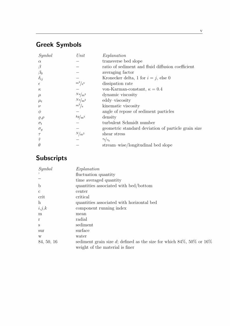
Symbol Unit Explanationα − transverse bed slopeβ − ratio of sediment and fluid diffusion coefficientβ0 − averaging factorδij − Kronecker delta, 1 for i = j, else 0ε m2/s3 dissipation rateκ − von-Karman-constant, κ = 0.4µ Ns/m2 dynamic viscosityµt
Ns/m2 eddy–viscosityν m2/s kinematic viscosityφ − angle of repose of sediment particles%,ρ kg/m3 densityσt − turbulent Schmidt numberσg − geometric standard deviation of particle grain sizeτ N/m2 shear stressτ − τb/τh
θ − stream–wise/longitudinal bed slope
Subscripts
Symbol Explanation’ fluctuation quantity
time averaged quantityb quantities associated with bed/bottomc centercrit criticalh quantities associated with horizontal bedi,j,k component running indexm meanr radials sedimentsur surfacew water84, 50, 16 sediment grain size d; defined as the size for which 84%, 50% or 16%
weight of the material is finer

vi
Abbreviations
Symbol Explanationcf. conferCFD Computational Fluid Dynamicse.g. exempli gratia (lat.) = for instanceeqn. equationet al. et alii (lat.) = et al.fig. figurei.e. id est (lat.) = that is to sayno. numberresp. respectivelySSIIM Sediment Simulation In Intakes with Multiblock optionSIMPLE Semi–Implicit Method for Pressure–Linked Equations
Contents
Statement ii
Abstract iii
Nomenclature iv
List of Figures ix
List of Tables ix
Acknowledgement x
1 Introduction 1
2 Fundamentals 22.1 Governing Equations for Water Flow Calculation . . . . . . . . . . . 22.2 Assumptions and Approximations . . . . . . . . . . . . . . . . . . . . 32.3 Governing Equations in Simplified Form . . . . . . . . . . . . . . . . 42.4 Turbulence Modelling . . . . . . . . . . . . . . . . . . . . . . . . . . . 5
2.4.1 Remarks . . . . . . . . . . . . . . . . . . . . . . . . . . . . . . 52.4.2 Reynold Stress Terms . . . . . . . . . . . . . . . . . . . . . . . 52.4.3 Boussinesq’s Approximation and Eddy–Viscosity . . . . . . . . 52.4.4 Eddy–diffusivity Concept . . . . . . . . . . . . . . . . . . . . . 62.4.5 The k–ε Turbulence Model . . . . . . . . . . . . . . . . . . . . 6
3 Sediment Transport Mechanism 83.1 Shields Parameter . . . . . . . . . . . . . . . . . . . . . . . . . . . . . 83.2 Incipient Motion of Sediment Particles on Generalized Sloping Fluvial
Beds . . . . . . . . . . . . . . . . . . . . . . . . . . . . . . . . . . . . 93.3 Transport Modes and Particle Motion Modes . . . . . . . . . . . . . . 103.4 Computation of Transport Quantities . . . . . . . . . . . . . . . . . . 11
3.4.1 Bed–Load Transport . . . . . . . . . . . . . . . . . . . . . . . 113.4.2 Suspended Load . . . . . . . . . . . . . . . . . . . . . . . . . . 13
4 Flow in Curved Open Channels 154.1 Secondary Flows . . . . . . . . . . . . . . . . . . . . . . . . . . . . . 154.2 Formation of Secondary Flows . . . . . . . . . . . . . . . . . . . . . . 154.3 Distribution of Longitudinal Velocity . . . . . . . . . . . . . . . . . . 174.4 Distribution of Vertical Velocity . . . . . . . . . . . . . . . . . . . . . 174.5 Effects on Sediment Transport . . . . . . . . . . . . . . . . . . . . . . 17
5 Numerical Model SSIIM 19
Contents viii
6 Description of Physical Model 206.1 Geometry and Flow Parameters . . . . . . . . . . . . . . . . . . . . . 206.2 Sediment Parameters . . . . . . . . . . . . . . . . . . . . . . . . . . . 22
7 Numerical Simulation 247.1 Represented Domain . . . . . . . . . . . . . . . . . . . . . . . . . . . 247.2 Presentation of Water Flow Results . . . . . . . . . . . . . . . . . . . 24
7.2.1 Basic Flow Configuration . . . . . . . . . . . . . . . . . . . . . 257.2.2 Secondary Flow . . . . . . . . . . . . . . . . . . . . . . . . . . 257.2.3 Distribution of Longitudinal Velocity . . . . . . . . . . . . . . 267.2.4 Distribution of Vertical Velocity . . . . . . . . . . . . . . . . . 287.2.5 Stream Separation and Formation of Recirculation Zone . . . 287.2.6 Concluding Remarks . . . . . . . . . . . . . . . . . . . . . . . 32
7.3 Presentation of Sediment Transport Results . . . . . . . . . . . . . . 327.3.1 Basic Sediment Configuration . . . . . . . . . . . . . . . . . . 337.3.2 Default Case . . . . . . . . . . . . . . . . . . . . . . . . . . . 337.3.3 Base Case . . . . . . . . . . . . . . . . . . . . . . . . . . . . . 357.3.4 Parameter Variation . . . . . . . . . . . . . . . . . . . . . . . 35
7.4 Uncertainties in Numerical Modelling . . . . . . . . . . . . . . . . . . 39
8 Conclusions and Outlook 41
A Listing C++ Subroutine 42
B Listing of Sediment Calculation Input File 44
C Photos 46
Bibliography 48
List of Figures
1 Definition sketch of angles θ and α . . . . . . . . . . . . . . . . . . . 102 Variation of τ with α according to Deys empirical equation . . . . . . 113 Dimensionless particle motion diagram . . . . . . . . . . . . . . . . . 124 Vertical distribution of sediment concentration according to Rouse [20] 145 Definition sketch of transverse inclination of surface and transverse
circulation at bend in channel . . . . . . . . . . . . . . . . . . . . . . 166 Definition sketch of channel shape seen from above . . . . . . . . . . 217 Definition sketch of channel shape seen from side . . . . . . . . . . . 218 Particle size distribution . . . . . . . . . . . . . . . . . . . . . . . . . 239 Definition sketch of mesh, top view . . . . . . . . . . . . . . . . . . . 2410 Definition sketch of cross–section, seen looking upstream . . . . . . . 2511 Velocity vector plot at cross-section no. F243 . . . . . . . . . . . . . . 2612 Position sketch of cross–sections . . . . . . . . . . . . . . . . . . . . . 2713 Longitudinal velocity distribution . . . . . . . . . . . . . . . . . . . . 2914 Horizontal velocity distribution (begin) . . . . . . . . . . . . . . . . . 3014 Horizontal velocity distribution (end) . . . . . . . . . . . . . . . . . . 3115 Sediment transport results conducting default case . . . . . . . . . . . 3416 Comparison of bed elevation changes between base case and experiment 3617 Bed elevation changes with regard to different bed roughness heights 3718 Sediment calculation with refined mesh and ∂t = 60s . . . . . . . . . 3819 Sediment calculations with distorted mesh at different time steps . . . 3920 Channel before experimental run . . . . . . . . . . . . . . . . . . . . 4621 Photo of channel bend showing one point bar . . . . . . . . . . . . . 4722 Photo of channel bend showing separated point bars . . . . . . . . . . 47
List of Tables
1 The values of the k–ε turbulence model [19]. . . . . . . . . . . . . . . 72 Computation time for a simulation time of ∆t = 4 h . . . . . . . . . . 37

Acknowledgement
This diploma thesis is the result of collaboration between the author, presently atthe Department of Hydraulic and Environmental Engineering in the Norwegian Uni-versity of Science and Technology (NTNU) and the author’s home department, theInstitute for Hydromechanics at the University of Karlsruhe (TH). The study hasbeen carried out at the Department of Hydraulic and Environmental Engineering,NTNU in summer 2004.
First of all I would like to thank both my supervisors at NTNU, Prof. Nils Rei-dar B. Olsen and Nils Ruther for their advice and support. They have always beenavailable and took time for discussion. Their help guided me through this work andled me to a deeper understanding of sediment engineering and computational fluiddynamics, which I appreciated very much. It has been a pleasure to work with them.
I would also like to mention with thanks the help of Ian Guymer and RichardDutton from the Department of Civil and Structural Engineering at the Universityof Sheffield. They provided me with all requested data from the physical experimentin order to carry out reasonable simulations and gave me advice during my work.
Furthermore, I would like to thank all the people at my working place and all themaster’s thesis students I met at the ’brakka’ during lunch time. I really enjoyedtheir warm welcome.
I also want to express my gratitude to all the people who encouraged and supportedmy request to go abroad during my final thesis at a foreign university.
And finally I am deeply indebted to my parents, who provided me with both moraland financial support during my period of study.
1 Introduction
Natural meandering rivers are very complex in their water flow situation. The streamis characterized by turbulent, strongly three-dimensional and irregular channel topog-raphy. Due to spiral motion, which is also known as secondary current or transversecirculation, the river tends to erode the outer bank, yielding deposits at the innerbank. These phenomena cause local scouring and local pooling. Important engi-neering efforts have been undertaken on rivers of all scales to stabilize the banklines.Therefore quantitative information with respect to erosion and deposition must bemade available for sound river management, e.g. for navigable river systems. Depo-sition of sediment in rivers may decrease the water depth, making navigation difficultor even impossible. But also erosion causes problems. For example, the Iffezheimbarrage on the Rhine River near Karlsruhe needs about 170, 000 m3 of sedimentsper year added artificially to avoid erosion in the downstream river bed. The costsamount to 5 million Euro each year [1].
Sediment transport modelling is an important tool for prediction as well as diagno-sis. Computer models permit the simulation and prediction of environmental impactssuch as river discharge, sediment grain size and its distribution and bed and bankformation.
In this thesis, the numerical sediment transport model SSIIM will be examined.The numerical results are tested against the measurement data taken from a physicalexperiment. A new algorithm to calculate the incipient motion of sediment particleson generalized sloping fluvial beds will be introduced as this is indispensable for arealistic simulation. This algorithm can adequately describe the threshold of sedimentmotion on a combined transverse and longitudinal sloping bed Dey [5]. Numericalparameters will be varied to test the sensitivity to the model results.
The results will be compared to measurements of the experimental run in order todetermine the capabilities and limitations of the numerical model SSIIM. Advantagesand disadvantages of SSIIM with respect to the reproduction of the physical processesand practical applications will be discussed.
The implementation of the additional sediment transport algorithm with the exist-ing CFD-code constitutes an improvement with regard to the prediction of sedimenttransport problems. SSIIM is able to make more reliable predictions and is thereforea useful tool for river, environmental and sedimentation engineering.
2 Fundamentals
2.1 Governing Equations for Water Flow Calculation
Conservation of Mass The law of conservation of mass states that mass can neitherbe destroyed nor created, but it can only be transformed by physical, chemical orbiological processes. All mass flow rates into a control volume through its controlsurface is equal to all mass flow rates out of the control volume plus the time changein mass inside the control volume. Written out fully in cartesian coordinates
∂%
∂t+
∂(%u)
∂x+
∂(%v)
∂y+
∂(%w)
∂z= 0, (2.1)
or generalizing to three dimensions, it can be written in Einsteinian notation ofrepeated indices
∂%
∂t+
∂(%ui)
∂xi
= 0, (2.2)
where % is the fluid density, t the time, ui the fluid velocity vector and xi is the positionvector. The index i replaces all three spatial dimensions and must be summed overall directions.
Conservation of Momentum The following Navier-Stokes equation represents the dif-ferential form of the law of conservation of momentum. It describes the motion of aflow particle at any time at any given position in the flow field. The equation canbe found in many textbooks [19, 22]. Using the Einsteinian notation and introduc-ing an additional index j, which again represents all three spatial dimensions, theNavier-Stokes equation can be written as
∂(%ui)
∂t+
∂(%uiuj)
∂xi
= − ∂p
∂xi
+∂τij
∂xi
+ fi, (2.3)
where p is the pressure and τij are the viscous stresses. Source and sink terms aresummerized in fi. These are acceleration due to gravity, buoyancy and external forcesby hydraulic structures, wave stresses, etc.
Transport Equation In a general flow, transport of solutes, salinity or heat are dueto advection and diffusion
∂C
∂t+
∂
∂xi
(uiC) = Em,i∂2C
∂x2i
+ Et,i∂2C
∂x2i
±KC, (2.4)
where C is the concentration of the dissolved substance or heat, Em is the molecular,Et the turbulent diffusion coefficient and KC represents a first-order reaction process.It should be mentioned that the diffusion coefficients have a constant value in each
2 Fundamentals 3
direction, but are not homogeneous with respect to their spatial direction and aretherefore non-isotropic. A derivation of (2.4) by using Fick’s law is given in Fischeret al. [7] and Socolofsky and Jirka [24].
Equation of State For sea water containing dissolved salt, the density % is a functionof temperature T , salinity S and the pressure p
% = f(T, S, p). (2.5)
2.2 Assumptions and Approximations
The following assumptions and approximations are applied in this study.
Incompressibility In river, environmental and sedimentation engineering, water flowsat low mach values. The effects of compressibility can be neglected.
Equation of state At a given temperature T and salinity S the fluid density is con-stant, assuming an incompressible fluid and small variations in topography. Also thedynamic viscosity µ is of constant value within the flow field.
Newtonian fluid For Newtonian isotropic fluids –like water considered in this study–the viscous stresses τij in (2.3) depend on the velocity gradients and can be formulatedas [22]
τij = µ
(∂ui
∂xj
+∂uj
∂xi
− 2
3δij
∂uk
∂xk
), (2.6)
where µ is a proportional factor called dynamic viscosity. The kinematic viscosityof the fluid, which is defined as the ratio of dynamic viscosity and the density, ν =µ%, depends also on the temperature T and pressure p. In the SSIIM software the
kinematic viscosity ν is hard–coded and can not be changed. It is equivalent to waterat 20°C, i.e. ν = 1.006 ·10−6 m2
s.
Reynolds decomposition With regard to turbulent flows, the instantaneous velocityui(xi, t) and pressure p(xi, t) can be decomposed in time–averaged mean velocityplus turbulent fluctuation, respectively in mean pressure plus turbulent fluctuation.Therefore, the resulting flow has a velocity and pressure such as
ui(xi, t) = ui(xi) + u′i(xi, t), (2.7a)
p(xi, t) = p(xi) + p′(xi, t), (2.7b)
where the overbar indicates the time–averaged mean and the prime the turbulentfluctuation quantities.
2 Fundamentals 4
The Reynolds-averaged equations are obtained if the Reynolds decomposition issubstituted into the basic equations (2.2) and (2.3). The resulting equations containfurther unknowns, namely the Reynolds stresses. These are new statistical correla-tions uiuj between different fluctuation velocities. A turbulence closure model de-scribes these quantities, which is introduced in more detail in chapter 2.4.Analogously, the other instantaneous quantities are also separated into their meanparts and a fluctuation from the mean. C(xi, t) = C(xi) + C ′(xi, t) is substitutedin (2.4). In natural streams, the magnitude for turbulent diffusion is several ordersgreater than molecular diffusion and can safely be removed from (2.4) (cf. Socolofskyand Jirka [24]). In this thesis, no reaction processes are considered and K is set atzero.
2.3 Governing Equations in Simplified Form
Invoking the restrictive conditions in chapter 2.2, the equations (2.2), (2.3) and (2.4)can be reduced to the following:
Conservation of Mass∂ui
∂xi
= 0 (2.8)
Momentum Equations or Reynolds Equations
∂ui
∂t+ uj
∂ui
∂xj
= − 1
%0
∂p
∂xi
+1
%0
∂
∂xj
(µ
∂ui
∂xj
− %0u′iu
′j
)+
fi
%0
(2.9)
where %0 is the reference density.
Transport Equation∂C
∂t+
∂
∂xi
(uiC) = Ei∂2C
∂x2i
(2.10)
Equation of state% = %0 = const. (2.11)
2.4 Turbulence Modelling
2.4.1 Remarks
Most flows which occur in practical river, environmental and sedimentation engineer-ing are turbulent, which means irregular fluctuation is superimposed on the mainmotion. Turbulence involves disorder, is irreproducable in detail, performs efficientmixing and transport and vorticity is irregularly distributed in all three spatial di-mensions. The large eddies are the main carriers of kinetic energy in the fluctuations.They obtain their energy from the mean motion. In a cascade process they decayand pass on their energy to several small eddies. At these smaller scales of motion,energy is dissipated by the action of viscosity, i.e. a transfer from mechanical en-ergy to internal energy. This observation is of great importance for the numericalmodelling of turbulence. To resolve these effects, a very fine grid is required. Thegrid represents the investigated natural hydraulic system in a numerical model. Forthat purpose the domain must be divided into cells. Because of the huge amount ofdata involved, it is only possible today to resolve the small-scale motions by directnumerical simulation (DNS) and the use of super-computers, which is not feasible forpractical engineering purposes. For this reason the effects of the smaller-scale motionon the main flow must be modelled.
2.4.2 Reynold Stress Terms
As already indicated in chapter 2.2, in computing a turbulent flow it is useful todecompose the instantaneous motion into mean and fluctuation velocity. The sameis done with the instantaneous pressure (cf. eqn. 2.7b). Substituting (2.7) into theNavier-Stokes Equation given in chapter (2.1) leads to the Reynolds-Equations (2.8)and (2.9). The only difference between these equations and (2.3) is the fluctuationpart; the term −%0u′
iu′j on the right side of (2.9). They cause an enhanced turbulent
momentum transport compared to the laminar flows and thus act like stresses. Theseterms are called Reynold stresses and are unknown. In order to be able to calculateturbulent flow, the system of equation must be supplemented by additional equationsfor these occurring unknowns. With regard to Schlichting and Gersten [22], trying toadd new terms for the unknowns will unfortunately lead to further unknowns in formof higher correlations, which would mean that closure of the system of equationsis never achieved. This is the so–called ’closure problem’ [22]. Therefore, modelequations must be used to connect the Reynold stresses to quantities of the meanflow.
2.4.3 Boussinesq’s Approximation and Eddy–Viscosity
Boussinesq’s eddy–viscosity concept suggested that in analogy to Newton’s law offriction, the turbulent stresses are proportional to the mean velocity gradients. For
2 Fundamentals 6
general flow situations, the turbulent stresses may be expressed as [19]
τij = −%uiuj = µt
(∂ui
∂xj
+∂uj
∂xi
)− 2
3%kδij (2.12)
It should be pointed out that µt(x, y, z, t) is not a physical property and not ofconstant value, but rather a function of position and time, i.e. it depends on the flowunder consideration. Consequently, the distribution of µt across the flow field mustbe estimated.
From dimensional analysis [19], the eddy–viscosity is proportional to three param-eters, namely
µt ∝ %V L, (2.13)
where V is a velocity-scale and L characterizes the large-scale turbulent motion. Thedistribution of these scales can be approximated reasonably well in many flows. Thecalculation of µt from the given parameters is described in chapter 2.4.5.
2.4.4 Eddy–diffusivity Concept
The relation between the eddy–viscosity and the turbulent diffusion coefficient Et isdescribed by the following equation
Et =µt
%σt
, (2.14)
where σt is the turbulent Schmidt–number.
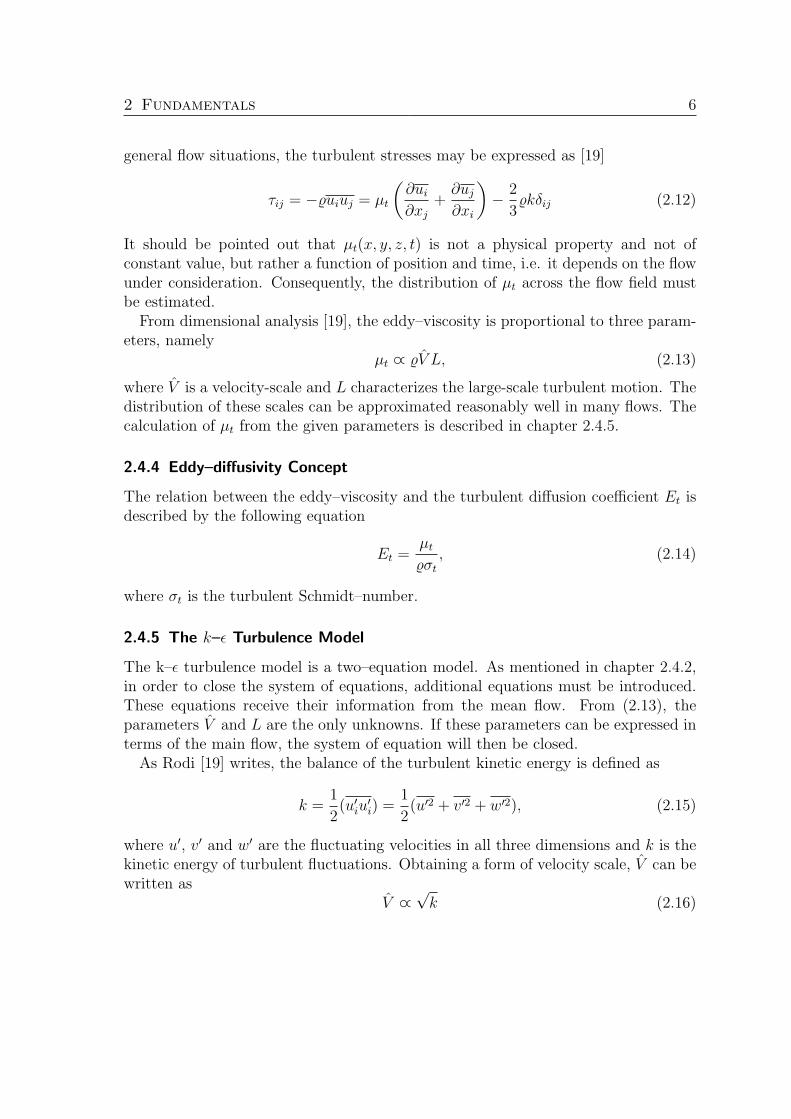
2.4.5 The k–ε Turbulence Model
The k–ε turbulence model is a two–equation model. As mentioned in chapter 2.4.2,in order to close the system of equations, additional equations must be introduced.These equations receive their information from the mean flow. From (2.13), theparameters V and L are the only unknowns. If these parameters can be expressed interms of the main flow, the system of equation will then be closed.
As Rodi [19] writes, the balance of the turbulent kinetic energy is defined as
k =1
2(u′
iu′i) =
1
2(u′2 + v′2 + w′2), (2.15)
where u′, v′ and w′ are the fluctuating velocities in all three dimensions and k is thekinetic energy of turbulent fluctuations. Obtaining a form of velocity scale, V can bewritten as
V ∝√
k (2.16)
2 Fundamentals 7
Table 1: The values of the k–ε turbulence model [19].
cµ c1 c2 σk σε
0.09 1.44 1.92 1.0 1.3
Dimensional considerations also allow defining a dissipation rate of turbulent en-ergy given by
ε ∝k
32
l∝
µ
%
∂u′i∂u′
i
∂xj∂xj
. (2.17)
Substituting (2.15) and (2.17) into (2.13), the k–ε model calculates the viscosityµt by
µt = f(k, ε) = cµ%k2
ε, (2.18)
where cµ is an empirical constant.In order to estimate the eddy–viscosity µt from (2.18), the distribution of k and
ε across the flow field must be known. The distribution can be calculated by themeans of transport equations k and ε. The modelled form according to Rodi [19] forthe turbulent kinetic energy k is
%∂k
∂t+ %ui
∂k
∂xi
=∂
∂xi
(µt
σk
∂k
∂xi
)+
∂ui
∂xj
(µt
(∂ui
∂xj
+∂uj
∂xi
))− %ε (2.19)
and the dissipation of k is denoted ε and modelled as
%∂ε
∂t+ %ui
∂ε
∂xi
=∂
∂xi
(µt
σε
∂ε
∂xi
)+ c1%
ε
k
∂ui
∂xj
(µt
(∂ui
∂xj
+∂uj
∂xi
))− c2%
ε2
k. (2.20)
The empirical constants given by Rodi [19] are shown in Table 1.The equations (2.19) and (2.20) in conjunction with (2.12), (2.9) and (2.10) describe
completely the k–ε model and allow the system of equations to be closed. Theempirical constants in Table 1 are determined by experiments. They are universalfor a wide range of flow situations. For this reason, the k–ε model is de–facto–standard in all industrial applications. Furthermore, the k–ε model shows a verystabil behaviour in numerical applications.
3 Sediment Transport Mechanism
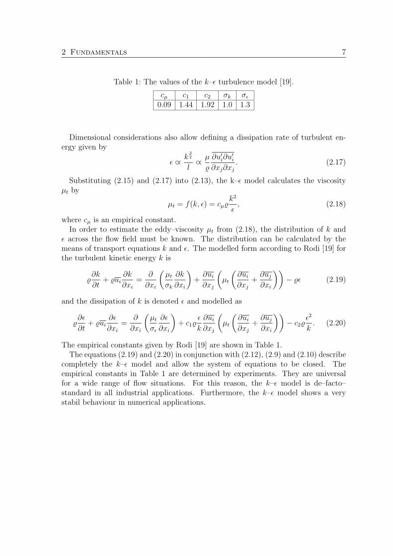
3.1 Shields Parameter
The river bed experiences shear stresses due to the flow of water. The classicaldeviation of the shear stress balances all forces acting on an element of the river.Taking all forces into account, produces the following equation (Zanke [29])
τ = %wgIeh, (3.1)
where τ is the shear stress, %w the density of water, g is acceleration due to gravity,Ie represents the energy slope and h is the flow depth.
A particle motion may be initiated by shear stress τ exceeding a critical value ofthe bed–shear stress τcrit, which is a function of sediment and hydraulic parameters[29],
τcrit = f(%s, %w, D, h, ν, g, I0), (3.2)
where %s the density of a sediment particle, %w is the density of water and ν itsviscosity coefficient, D the mean particle size, h water depth and I0 represents thechannel slope. Since the flow under consideration is uniform and steady, the energy-and channel slope are of equal value, Ie=I0.
Shields [23] investigated the value of τcrit by the means of flume experiments, usingbed material of uniform size. Applying the Buckingham Π–Theorem (cf. Zanke [29]),these seven basic parameters can be reduced to a set of four dimensionless parameters,which are:
1. Specific density parameter
s =%s
%w
, (3.3)
2. depth-particle size ratioh
D, (3.4)
3. particle Reynolds–number
Re∗ =u∗D
ν, (3.5)
where u∗ is the bed–shear velocity, defined as u∗ =√
τ%w
, and
4. particle Froude–number, defined as the ratio of the frictional load on the grainto the gravitational force on the grain that resists movement
τ∗ = Fr∗ =u2∗
(s− 1)gD=
τ
(%s − %w)gD. (3.6)
3 Sediment Transport Mechanism 9
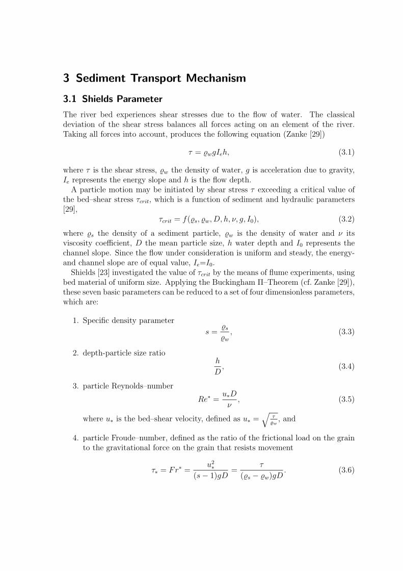
The empirical dimensionless parameter Fr∗ can be taken from the Shields’ diagramfound in many textbooks [9, 10, 23], where Fr∗ is a function of Re∗. The Shields’relationship between dimensionless shear stress Fr∗ (or Shields parameter τ∗) andparticle Reynolds–number Re∗ can be applied for predicting whether or not a particlewill move. The dimensionless value of τ∗,crit = 0.03 to 0.06 is often used as a limitfor bed protection. If the value of bed–shear τ exceeds the critical value τcrit, motionwill be initiated, expressed by following dimensionless expression
τ∗ > τ∗,crit. (3.7)
3.2 Incipient Motion of Sediment Particles on GeneralizedSloping Fluvial Beds
The above chapter describes the forces induced by the flow acting on sediment parti-cles and its prediction of initial movement. The Shields’ curve has been introduced.Shields was the pioneer who described the incipient motion of uniform sediment par-ticles. For his investigations he used two different types of rectangular flow channels.On the one hand a wooden channel 0.8m in width, on the other hand a channel madeout of glass and 0.4m in width. This one could be inclined in a longitudinal direc-tion [9]. Although Shields’ approach is widely used, it has disadvantages. Shields’diagram is limited to bed slopes close to zero and can not be used in channels havingsubstantial bed slope [6]. It is also limited to stream flows without transverse incli-nation.In the further study of this thesis a flow in a trapezoidal channel bed is investigated.The geometry is not rectangular because of the inclination of the inner and outerbank. A modified form of the Shields’ approach has to be found, in order to take theeffects of a combined transverse and longitudinal sloping bed on a sediment particleinto account.
Dey [5] reports experimental results on incipient motion of non–cohesive, uniformsediment particles under an unidirectional steady–uniform flow on generalized slopingbeds. He gives a formulation of particle stability by presenting the non–dimensionalratio τ of critical shear stress on a generalized sloping bed τb compared with thecritical shear stress on a horizontal bed τh, yielding
τ =τb
τh
. (3.8)
From dimensional analysis it can be shown:
τ = f(φ, θ, α), (3.9)
where φ is the angle of repose of sediment particles, θ is the stream–wise bed slopeand α is the transverse bed slope, as depicted in Fig. 1. Conducting experiments,
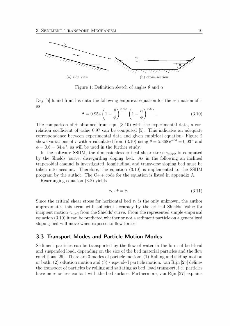
3 Sediment Transport Mechanism 10
(a) side view (b) cross–section
Figure 1: Definition sketch of angles θ and α
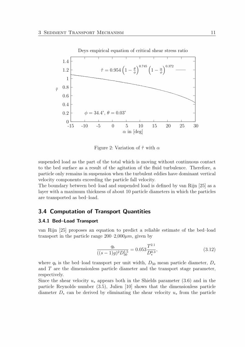
Dey [5] found from his data the following empirical equation for the estimation of τas
τ = 0.954
(1− θ
φ
)0.745(1− α
φ
)0.372
. (3.10)
The comparison of τ obtained from eqn. (3.10) with the experimental data, a cor-relation coefficient of value 0.97 can be computed [5]. This indicates an adequatecorrespondence between experimental data and given empirical equation. Figure 2shows variations of τ with α calculated from (3.10) using θ = 5.368 e−04 = 0.03 ◦ andφ = 0.6 = 34.4 ◦, as will be used in the further study.
In the software SSIIM, the dimensionless critical shear stress τ∗,crit is computedby the Shields’ curve, disregarding sloping bed. As in the following an inclinedtrapezoidal channel is investigated, longitudinal and transverse sloping bed must betaken into account. Therefore, the equation (3.10) is implemented to the SSIIMprogram by the author. The C++ code for the equation is listed in appendix A.
Rearranging equation (3.8) yields
τh · τ = τb. (3.11)
Since the critical shear stress for horizontal bed τh is the only unknown, the authorapproximates this term with sufficient accuracy by the critical Shields’ value forincipient motion τ∗,crit from the Shields’ curve. From the represented simple empiricalequation (3.10) it can be predicted whether or not a sediment particle on a generalizedsloping bed will move when exposed to flow forces.
3.3 Transport Modes and Particle Motion Modes
Sediment particles can be transported by the flow of water in the form of bed–loadand suspended load, depending on the size of the bed material particles and the flowconditions [25]. There are 3 modes of particle motion: (1) Rolling and sliding motionor both, (2) saltation motion and (3) suspended particle motion. van Rijn [25] definesthe transport of particles by rolling and saltating as bed–load transport, i.e. particleshave more or less contact with the bed surface. Furthermore, van Rijn [27] explains
3 Sediment Transport Mechanism 11
0
0.2
0.4
0.6
0.8
1
1.2
1.4
-15 -10 -5 0 5 10 15 20 25 30
τ
α in [deg]
Deys empirical equation of critical shear stress ratio
φ = 34.4°, θ = 0.03°
τ = 0.954(1− θ
φ
)0.745 (1− α
φ
)0.372
Figure 2: Variation of τ with α
suspended load as the part of the total which is moving without continuous contactto the bed surface as a result of the agitation of the fluid turbulence. Therefore, aparticle only remains in suspension when the turbulent eddies have dominant verticalvelocity components exceeding the particle fall velocity.The boundary between bed–load and suspended load is defined by van Rijn [25] as alayer with a maximum thickness of about 10 particle diameters in which the particlesare transported as bed–load.
3.4 Computation of Transport Quantities
3.4.1 Bed–Load Transport
van Rijn [25] proposes an equation to predict a reliable estimate of the bed–loadtransport in the particle range 200–2,000µm, given by
qb
((s− 1)g)2D1.550
= 0.053T 2.1
D0.3∗
, (3.12)
where qb is the bed–load transport per unit width, D50 mean particle diameter, D∗and T are the dimensionless particle diameter and the transport stage parameter,respectively.Since the shear velocity u∗ appears both in the Shields parameter (3.6) and in theparticle Reynolds–number (3.5), Julien [10] shows that the dimensionless particlediameter D∗ can be derived by eliminating the shear velocity u∗ from the particle
3 Sediment Transport Mechanism 12
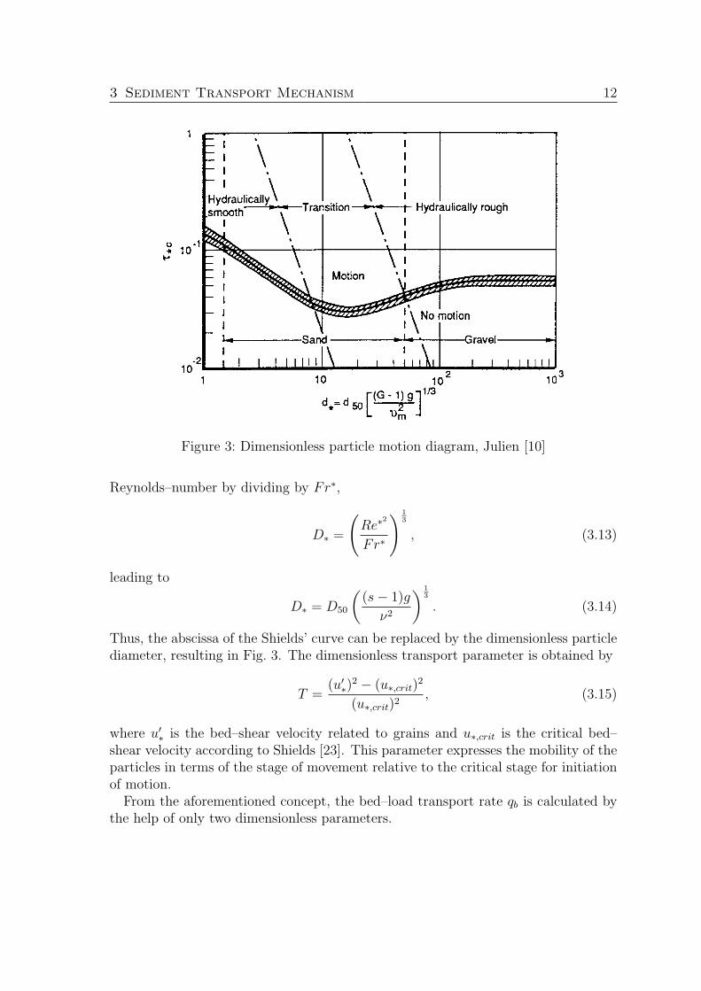
Figure 3: Dimensionless particle motion diagram, Julien [10]
Reynolds–number by dividing by Fr∗,
D∗ =
(Re∗
2
Fr∗
) 13
, (3.13)
leading to
D∗ = D50
((s− 1)g
ν2
) 13
. (3.14)
Thus, the abscissa of the Shields’ curve can be replaced by the dimensionless particlediameter, resulting in Fig. 3. The dimensionless transport parameter is obtained by
T =(u′
∗)2 − (u∗,crit)
2
(u∗,crit)2, (3.15)
where u′∗ is the bed–shear velocity related to grains and u∗,crit is the critical bed–
shear velocity according to Shields [23]. This parameter expresses the mobility of theparticles in terms of the stage of movement relative to the critical stage for initiationof motion.
From the aforementioned concept, the bed–load transport rate qb is calculated bythe help of only two dimensionless parameters.
3 Sediment Transport Mechanism 13
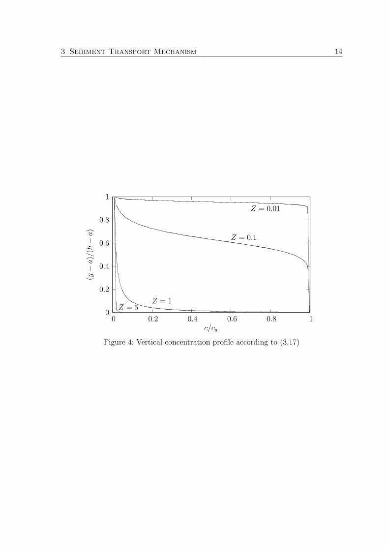
3.4.2 Suspended Load
Sediment particles are transported as suspended load, if the upward turbulent fluidforces exceed the downward gravitational forces. van Rijn [26] uses the suspensionparameter Z by Rouse [20], expressing the influence of the above–mentioned forces,yielding
Z =ws
βκu∗, (3.16)
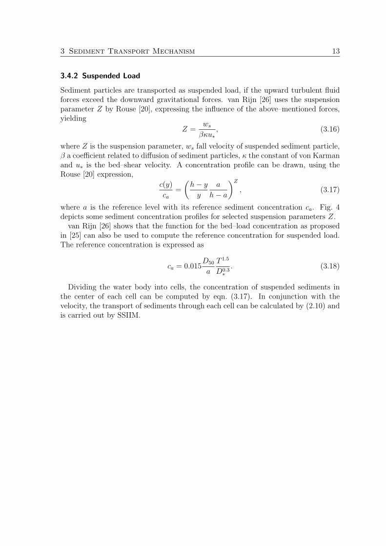
where Z is the suspension parameter, ws fall velocity of suspended sediment particle,β a coefficient related to diffusion of sediment particles, κ the constant of von Karmanand u∗ is the bed–shear velocity. A concentration profile can be drawn, using theRouse [20] expression,
c(y)
ca
=
(h− y
y
a
h− a
)Z
, (3.17)
where a is the reference level with its reference sediment concentration ca. Fig. 4depicts some sediment concentration profiles for selected suspension parameters Z.
van Rijn [26] shows that the function for the bed–load concentration as proposedin [25] can also be used to compute the reference concentration for suspended load.The reference concentration is expressed as
ca = 0.015D50
a
T 1.5
D0.3∗
. (3.18)
Dividing the water body into cells, the concentration of suspended sediments inthe center of each cell can be computed by eqn. (3.17). In conjunction with thevelocity, the transport of sediments through each cell can be calculated by (2.10) andis carried out by SSIIM.
3 Sediment Transport Mechanism 14
0
0.2
0.4
0.6
0.8
1
0 0.2 0.4 0.6 0.8 1
(y−
a)/
(h−
a)
c/ca
Z = 5Z = 1
Z = 0.1
Z = 0.01
Figure 4: Vertical concentration profile according to (3.17)
4 Flow in Curved Open Channels
4.1 Secondary Flows
Secondary flows are defined as currents that occur in the plane normal to the primaryflow direction. Their velocities are typically one order of magnitude smaller than thebulk primary velocity [2]. Ciray [4] gives a rather functional definition on secondaryflows as follows: ”When the magnitude of the vector composed by any two compo-nents [of] the local velocity vector[s] in a three dimensional flow is small comparedwith the magnitude of the third component, the latter forms the main flow whereasthe remaining two form the secondary.”
Nevertheless, secondary currents strongly influence the velocity pattern of thestream. Different velocity patterns in cross–streamwise and vertical direction of theflow will be found. Secondary currents combined with the primary flow produce aspiral flow rotating around the primary flow direction and therefore affect the pro-cesses of flow resistance, sediment transport, bed and bank erosion and developmentof channel morphology [2].
Prandtl et al. [18] distinguishes three modes of secondary flows by the releasingforces. In the present study the secondary flow of the first type will be discussed asit is of interest to flows under consideration. These secondary flows of the first modeare provoked by differences in centrifugal forces.
4.2 Formation of Secondary Flows
Rozovskii [21] gives an explanation of the formation of secondary currents. He con-siders an open stream that moves first in a straight channel and then passes into acurvature. From currents being curved on a plane, the appearance of a transverseinclination of the free surface can be observed. To evaluate approximately the extentof this inclination Ir, centrifugal-, pressure- and friction forces are balanced, yielding
Ir =dh
dr= βo
v2cm
grc
+τrb
%gh, (4.1)
where h is the water depth, rc is the radius at the center of the bend, τrb the radialcomponent of the friction stress at the bottom and vcm is the mean velocity. Sincethe vertical velocity is unevenly distributed over the depth, an averaging factor β0 isintroduced to estimate the average velocity in streamwise direction.As the friction term τrb
%ghon the right side of (4.1) is in many cases of small quantity,
it can be omitted. Thus the approximate equation for the inclination of the watersurface is obtained as
Ir =dh
dr= βo
v2cm
grc
. (4.2)
4 Flow in Curved Open Channels 16
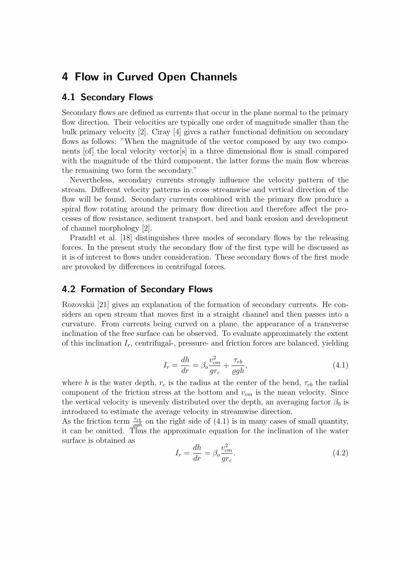
Figure 5: Definition sketch of transverse inclination of surface and transverse circu-lation at bend in channel [21], a–section AB; b–plan
Eqn. (4.2) shows that at any bending of a stream on a plane, a transverse inclinationinevitable appears. The level of the free surface at the inner bank, which is nearest tothe center of the turn, will decrease. The reverse at the outer bank, which is farthestfrom the center of the turn, will have an increasing water level. To conform to thetechnical literature, the inner bank will be termed in the rest of this text the ”convexbank”, and the outer bank the ”concave bank”.
Another characteristic property of a flow passing a bend is the presence of trans-verse circulation. Rozovskii [21] considers a volume element at a distance z from thebottom, which moves along the circular trajectories of an equal radius r as shown inFigure 5. With the absence of radial velocity components, the friction force is takenas zero. Again, balancing all forces acting on the volume element leads to
Ir =dh
dr=
v2
gr. (4.3)
As (4.2) and (4.3) describe the identical phenomena, Ir must be equal in both cases.This is achieved only in two cases: first, in a straight channel, where r = ∞, andsecond, where v2 of (4.3) is of constant value and equals β0v
2cm of (4.2), i.e. a uniform
distribution of the velocity along the vertical. It is well known that due to frictionat the boundaries of the stream, the velocity at the bottom and at the walls areminimum. Close to the water surface they are maximum. The velocities thereforecan not be of constant value, but deviate from the mean, depending on their positionin the flow. Owing to variations in vertical velocity, the averaging factor β0 wasintroduced in (4.1), so the term v2 can not be of constant value. For particles movingnear the upper surface with a velocity faster than the mean of the flow, centrifugalforces will be greater than the pressure forces. These particles will consequentlybe displaced in a radial direction towards the concave bank. For the same reason,particles in the lower part of the stream will move toward the convex bank. Particlesreaching the wall will move in a down- or upward direction, producing a circulation.
4 Flow in Curved Open Channels 17
To conclude, simultaneously with the radial displacement, a vertical velocity com-ponent also appears, i.e. a flow in the transverse direction, also called transversecirculation. It is obvious from the above–mentioned that in bending streams, atransverse circulation is superimposed on the main flow direction and a flow passinga bend is of a complex spatial character.
4.3 Distribution of Longitudinal Velocity
Owing to basic flow superimposed by a transverse circulation, the velocity structureof a stream within a bend is subjected to strong changes. A stream which movesfirst in a straight, uniform channel will have its maximum longitudinal velocity inthe middle of the channel width. Entering the bend, the maximum velocity movestowards the convex bank [21]. As aforementioned, by virtue of centrifugal forcesacting on fluid elements in the same way, but varying in its magnitude at differentdepths, a transverse slope on the free surface appears. The level at the convex banklowers, while rising at the concave bank. The amount of transverse slope can bedetermined with sufficient accuracy from (4.2), taking β0 = 1.
By lowering the free surface at the convex bank, the velocity is increased due to asmaller flow area perpendicular to the main flow direction. This is stated by the lawof conservation of mass in (2.1). If the level of the free surface rises, a simultaneousdecrease in velocity must take place.
If the secondary flow fully develops in the bend, an interchange of momentumbetween horizontal currents takes place by reason of transverse circulation. As aconsequence, the maximum velocity moves from the convex to the concave bank [21].
4.4 Distribution of Vertical Velocity
A change in current velocity is not only limited to longitudinal direction. Also in thevertical direction, a movement of the velocity maximum can be observed. It tendsto compensate the velocity differences in the vertical direction, so that the maximumvelocity in the longitudinal direction not only moves from the convex to the concavebank, but also from the near-surface to the near-bottom. It is also worth mentioningthat the typical logarithmic velocity profile as found in straight channels does nothold true in bends [13].
4.5 Effects on Sediment Transport
From a morphological point of view, high bed–shear stresses, high velocities and itsinhomogenity of distribution exert great influence on the water and material transportproperties of a stream.Increasing velocity near the bed in the direction of primary flow are responsible forenhanced sediment transport in bends. The direction of sediment motion follows the

4 Flow in Curved Open Channels 18
resulting force of primary and transverse shear stress components. The secondary flownear the bed leads to erosion at the concave bank and to deposition at the convexbank, resulting in a scour and a point bar. Owing to these effects, the transversebed slope increases and stability of bed material decreases as threshold conditionsfor incipient motion changes (cf. chapter 3.2). The morphological processes showdynamical behaviour. Secondary flows, with their complex structure in time andspace, need three–dimensional models if investigated in more detail.
5 Numerical Model SSIIM 19
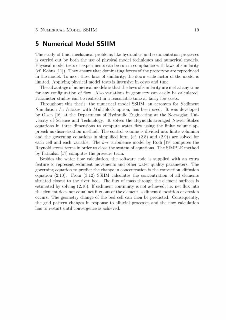
5 Numerical Model SSIIM
The study of fluid mechanical problems like hydraulics and sedimentation processesis carried out by both the use of physical model techniques and numerical models.Physical model tests or experiments can be run in compliance with laws of similarity(cf. Kobus [11]). They ensure that dominating forces of the prototype are reproducedin the model. To meet these laws of similarity, the down-scale factor of the model islimited. Applying physical model tests is intensive in costs and time.
The advantage of numerical models is that the laws of similarity are met at any timefor any configuration of flow. Also variations in geometry can easily be calculated.Parameter studies can be realized in a reasonable time at fairly low costs.
Throughout this thesis, the numerical model SSIIM, an acronym for SedimentS imulation In Intakes with Multiblock option, has been used. It was developedby Olsen [16] at the Department of Hydraulic Engineering at the Norwegian Uni-versity of Science and Technology. It solves the Reynolds-averaged Navier-Stokesequations in three dimensions to compute water flow using the finite volume ap-proach as discretization method. The control volume is divided into finite voluminaand the governing equations in simplified form (cf. (2.8) and (2.9)) are solved foreach cell and each variable. The k–ε turbulence model by Rodi [19] computes theReynold stress terms in order to close the system of equations. The SIMPLE methodby Patankar [17] computes the pressure term.
Besides the water flow calculation, the software code is supplied with an extrafeature to represent sediment movements and other water quality parameters. Thegoverning equation to predict the change in concentration is the convection–diffusionequation (2.10). From (3.12) SSIIM calculates the concentration of all elementssituated closest to the river–bed. The flux of mass through the element surfaces isestimated by solving (2.10). If sediment continuity is not achieved, i.e. net flux intothe element does not equal net flux out of the element, sediment deposition or erosionoccurs. The geometry change of the bed cell can then be predicted. Consequently,the grid pattern changes in response to alluvial processes and the flow calculationhas to restart until convergence is achieved.
6 Description of Physical Model
6.1 Geometry and Flow Parameters
The physical model was originally used for experimental studies on longitudinal dis-persion tests at the University of Sheffield. Besides this main research, at differentlocations in the channel, measurements of the geometry have been registered andrepeated at different time intervals, in order to document the evolution of the bedtopography. Collected data [8]are unpublished and have been kindly contributed tothe author. These data are of great interest. It is indispensable to compare resultspredicted by SSIIM with experimental data to validate the sediment transport fea-ture of the program. Because of the availability of experimental data, this case ischosen to test the sediment transport prediction of SSIIM.
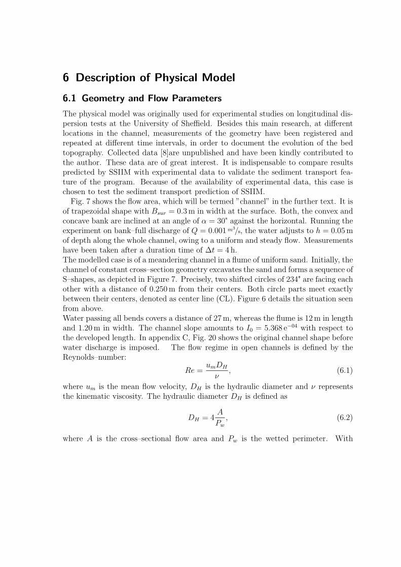
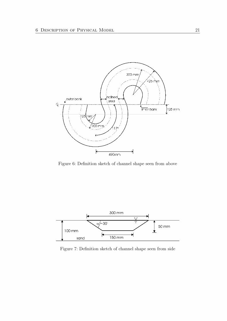
Fig. 7 shows the flow area, which will be termed ”channel” in the further text. It isof trapezoidal shape with Bsur = 0.3 m in width at the surface. Both, the convex andconcave bank are inclined at an angle of α = 30° against the horizontal. Running theexperiment on bank–full discharge of Q = 0.001 m3/s, the water adjusts to h = 0.05 mof depth along the whole channel, owing to a uniform and steady flow. Measurementshave been taken after a duration time of ∆t = 4 h.The modelled case is of a meandering channel in a flume of uniform sand. Initially, thechannel of constant cross–section geometry excavates the sand and forms a sequence ofS–shapes, as depicted in Figure 7. Precisely, two shifted circles of 234° are facing eachother with a distance of 0.250 m from their centers. Both circle parts meet exactlybetween their centers, denoted as center line (CL). Figure 6 details the situation seenfrom above.Water passing all bends covers a distance of 27 m, whereas the flume is 12 m in lengthand 1.20 m in width. The channel slope amounts to I0 = 5.368 e−04 with respect tothe developed length. In appendix C, Fig. 20 shows the original channel shape beforewater discharge is imposed. The flow regime in open channels is defined by theReynolds–number:
Re =umDH
ν, (6.1)
where um is the mean flow velocity, DH is the hydraulic diameter and ν representsthe kinematic viscosity. The hydraulic diameter DH is defined as
DH = 4A
Pw
, (6.2)
where A is the cross–sectional flow area and Pw is the wetted perimeter. With
6 Description of Physical Model 21
Figure 6: Definition sketch of channel shape seen from above
Figure 7: Definition sketch of channel shape seen from side
6 Description of Physical Model 22
h = 0.05 m, α = 30° and Bb = 0.1268 m,
A = h(Bb + h cot α) = 0.01067 m2 (6.3a)
and Pw = Bb +2h
sin α= 0.3268 m (6.3b)
resulting in DH = = 0.1306 m, (6.3c)
the mean Reynolds–number is calculated to
Re ≈ 12.000 > 2000, (6.4)
with um = Q/A = 0.093721 m/s. The flow under consideration is therefore turbulent.Introducing the Froude–number as
Fr =um√
g (A/Bsur), (6.5)
where Bsur is the width of the water surface, yields in
Fr = 0.16 < 1, (6.6)
low kinetic energy or subcritical flow.
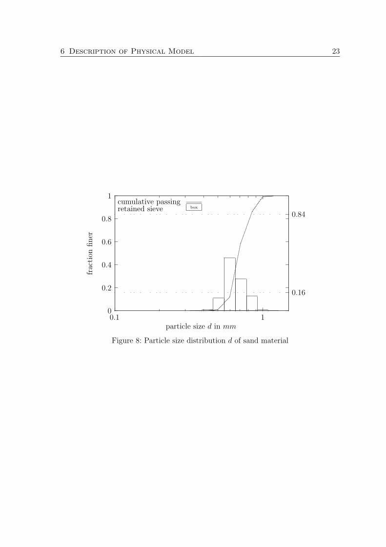
6.2 Sediment Parameters
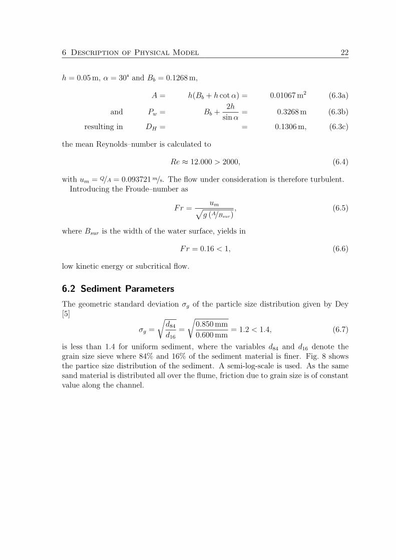
The geometric standard deviation σg of the particle size distribution given by Dey[5]
σg =
√d84
d16
=
√0.850 mm
0.600 mm= 1.2 < 1.4, (6.7)
is less than 1.4 for uniform sediment, where the variables d84 and d16 denote thegrain size sieve where 84% and 16% of the sediment material is finer. Fig. 8 showsthe partice size distribution of the sediment. A semi-log-scale is used. As the samesand material is distributed all over the flume, friction due to grain size is of constantvalue along the channel.
6 Description of Physical Model 23
0
0.2
0.4
0.6
0.8
1
0.1 1
0.84
0.16
frac
tion
finer
particle size d in mm
cumulative passingretained sieve box
Figure 8: Particle size distribution d of sand material
7 Numerical Simulation
7.1 Represented Domain
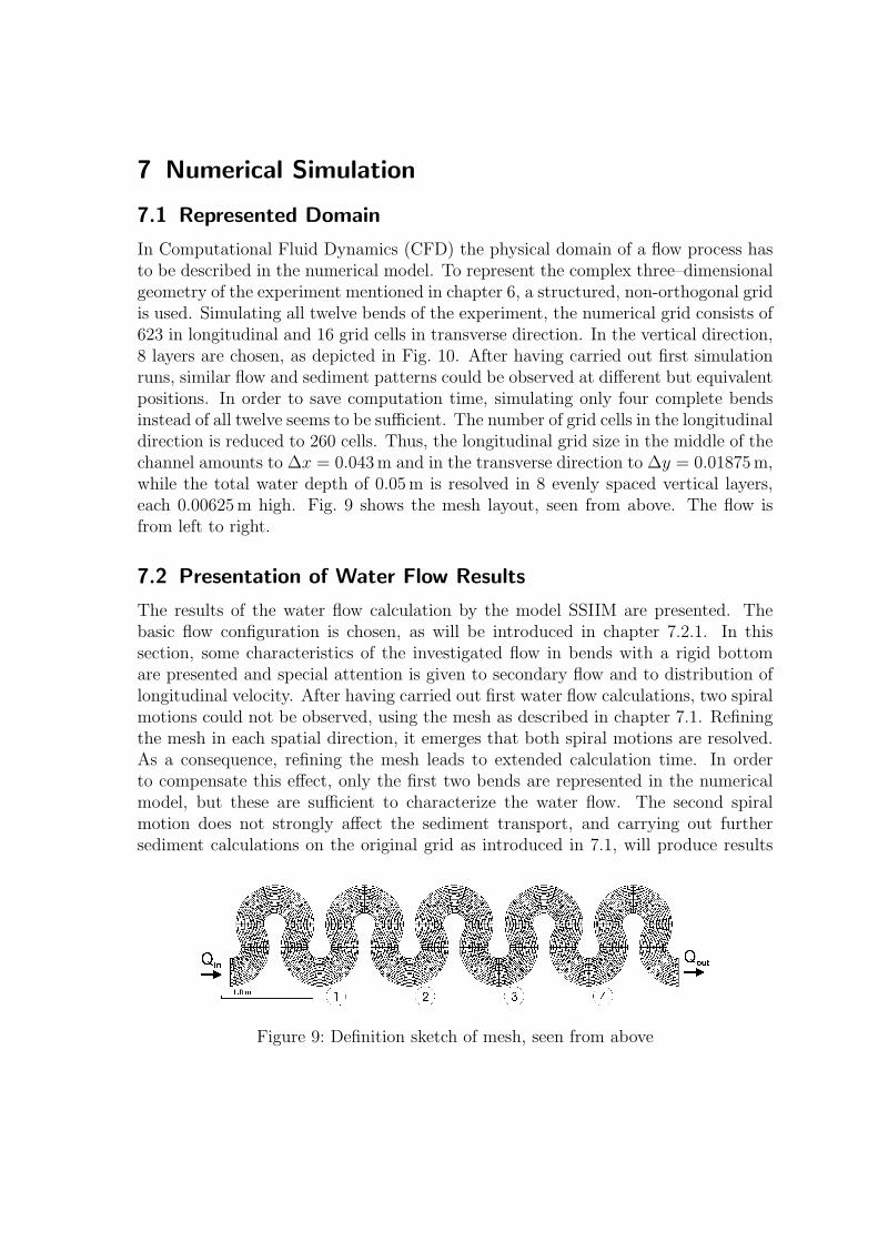
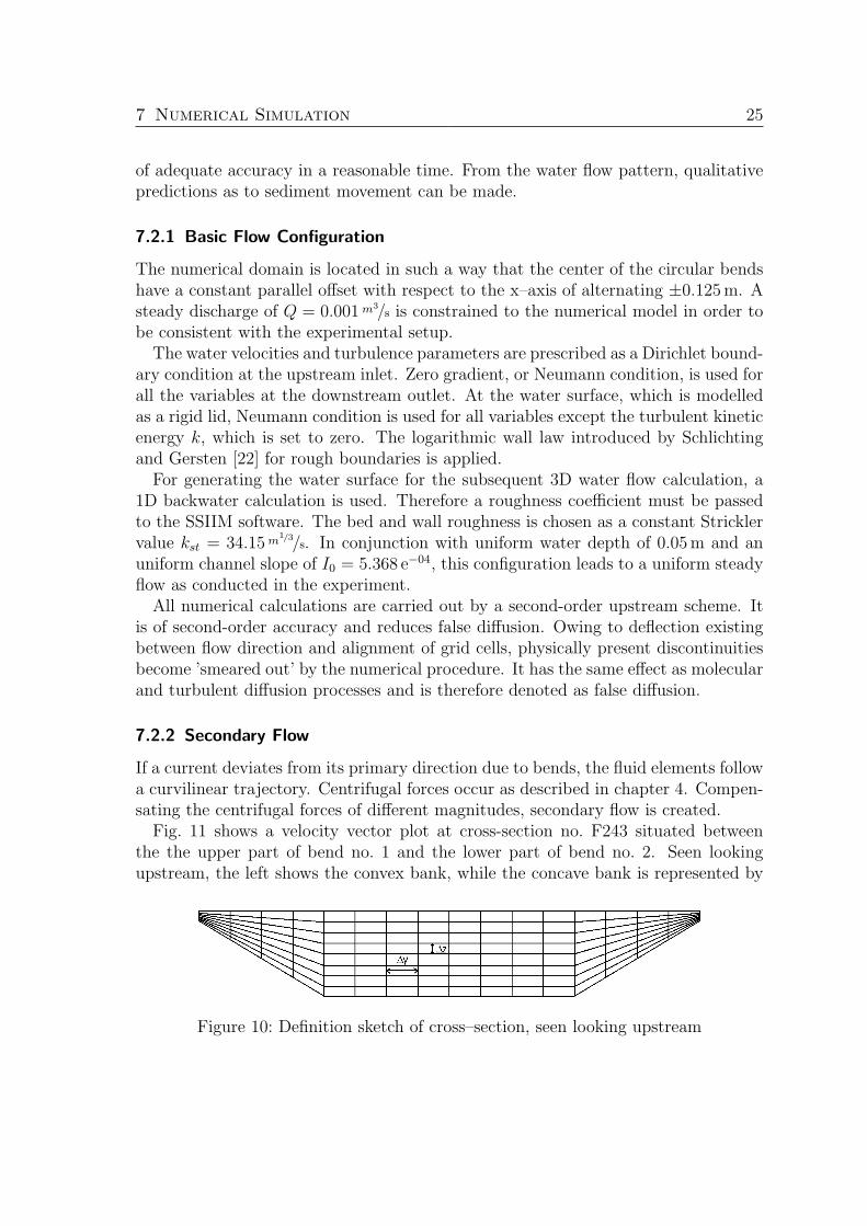
In Computational Fluid Dynamics (CFD) the physical domain of a flow process hasto be described in the numerical model. To represent the complex three–dimensionalgeometry of the experiment mentioned in chapter 6, a structured, non-orthogonal gridis used. Simulating all twelve bends of the experiment, the numerical grid consists of623 in longitudinal and 16 grid cells in transverse direction. In the vertical direction,8 layers are chosen, as depicted in Fig. 10. After having carried out first simulationruns, similar flow and sediment patterns could be observed at different but equivalentpositions. In order to save computation time, simulating only four complete bendsinstead of all twelve seems to be sufficient. The number of grid cells in the longitudinaldirection is reduced to 260 cells. Thus, the longitudinal grid size in the middle of thechannel amounts to ∆x = 0.043 m and in the transverse direction to ∆y = 0.01875 m,while the total water depth of 0.05 m is resolved in 8 evenly spaced vertical layers,each 0.00625 m high. Fig. 9 shows the mesh layout, seen from above. The flow isfrom left to right.
7.2 Presentation of Water Flow Results
The results of the water flow calculation by the model SSIIM are presented. Thebasic flow configuration is chosen, as will be introduced in chapter 7.2.1. In thissection, some characteristics of the investigated flow in bends with a rigid bottomare presented and special attention is given to secondary flow and to distribution oflongitudinal velocity. After having carried out first water flow calculations, two spiralmotions could not be observed, using the mesh as described in chapter 7.1. Refiningthe mesh in each spatial direction, it emerges that both spiral motions are resolved.As a consequence, refining the mesh leads to extended calculation time. In orderto compensate this effect, only the first two bends are represented in the numericalmodel, but these are sufficient to characterize the water flow. The second spiralmotion does not strongly affect the sediment transport, and carrying out furthersediment calculations on the original grid as introduced in 7.1, will produce results
Figure 9: Definition sketch of mesh, seen from above
7 Numerical Simulation 25
of adequate accuracy in a reasonable time. From the water flow pattern, qualitativepredictions as to sediment movement can be made.
7.2.1 Basic Flow Configuration
The numerical domain is located in such a way that the center of the circular bendshave a constant parallel offset with respect to the x–axis of alternating ±0.125 m. Asteady discharge of Q = 0.001 m3/s is constrained to the numerical model in order tobe consistent with the experimental setup.
The water velocities and turbulence parameters are prescribed as a Dirichlet bound-ary condition at the upstream inlet. Zero gradient, or Neumann condition, is used forall the variables at the downstream outlet. At the water surface, which is modelledas a rigid lid, Neumann condition is used for all variables except the turbulent kineticenergy k, which is set to zero. The logarithmic wall law introduced by Schlichtingand Gersten [22] for rough boundaries is applied.
For generating the water surface for the subsequent 3D water flow calculation, a1D backwater calculation is used. Therefore a roughness coefficient must be passedto the SSIIM software. The bed and wall roughness is chosen as a constant Stricklervalue kst = 34.15 m
1/3/s. In conjunction with uniform water depth of 0.05 m and anuniform channel slope of I0 = 5.368 e−04, this configuration leads to a uniform steadyflow as conducted in the experiment.
All numerical calculations are carried out by a second-order upstream scheme. Itis of second-order accuracy and reduces false diffusion. Owing to deflection existingbetween flow direction and alignment of grid cells, physically present discontinuitiesbecome ’smeared out’ by the numerical procedure. It has the same effect as molecularand turbulent diffusion processes and is therefore denoted as false diffusion.
7.2.2 Secondary Flow
If a current deviates from its primary direction due to bends, the fluid elements followa curvilinear trajectory. Centrifugal forces occur as described in chapter 4. Compen-sating the centrifugal forces of different magnitudes, secondary flow is created.
Fig. 11 shows a velocity vector plot at cross-section no. F243 situated betweenthe the upper part of bend no. 1 and the lower part of bend no. 2. Seen lookingupstream, the left shows the convex bank, while the concave bank is represented by
Figure 10: Definition sketch of cross–section, seen looking upstream
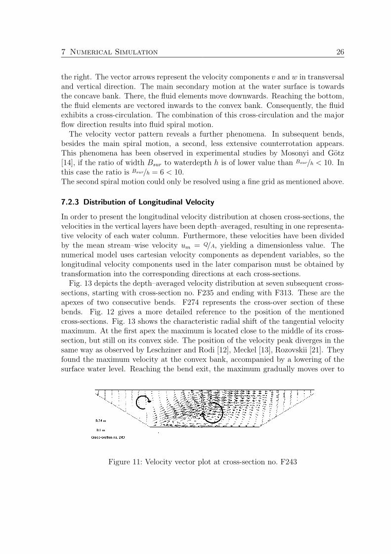
7 Numerical Simulation 26
the right. The vector arrows represent the velocity components v and w in transversaland vertical direction. The main secondary motion at the water surface is towardsthe concave bank. There, the fluid elements move downwards. Reaching the bottom,the fluid elements are vectored inwards to the convex bank. Consequently, the fluidexhibits a cross-circulation. The combination of this cross-circulation and the majorflow direction results into fluid spiral motion.
The velocity vector pattern reveals a further phenomena. In subsequent bends,besides the main spiral motion, a second, less extensive counterrotation appears.This phenomena has been observed in experimental studies by Mosonyi and Gotz[14], if the ratio of width Bsur to waterdepth h is of lower value than Bsur/h < 10. Inthis case the ratio is Bsur/h = 6 < 10.The second spiral motion could only be resolved using a fine grid as mentioned above.
7.2.3 Distribution of Longitudinal Velocity
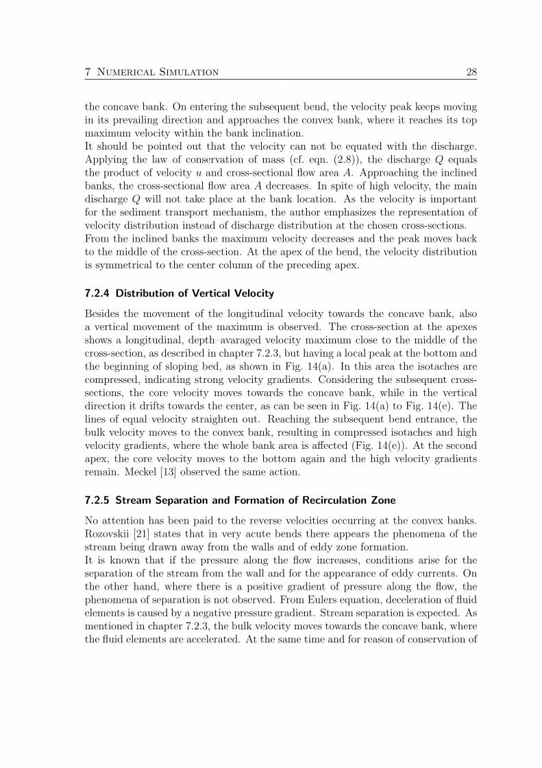
In order to present the longitudinal velocity distribution at chosen cross-sections, thevelocities in the vertical layers have been depth–averaged, resulting in one representa-tive velocity of each water column. Furthermore, these velocities have been dividedby the mean stream–wise velocity um = Q/A, yielding a dimensionless value. Thenumerical model uses cartesian velocity components as dependent variables, so thelongitudinal velocity components used in the later comparison must be obtained bytransformation into the corresponding directions at each cross-sections.
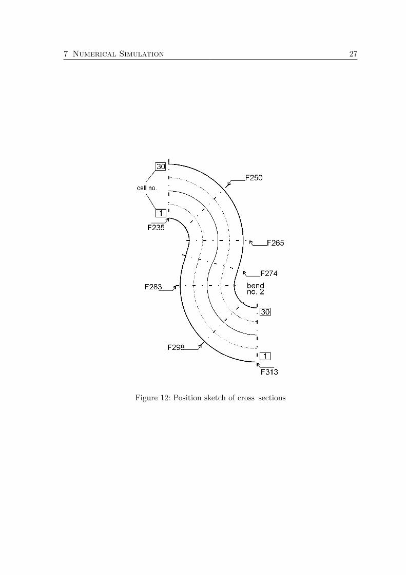
Fig. 13 depicts the depth–averaged velocity distribution at seven subsequent cross-sections, starting with cross-section no. F235 and ending with F313. These are theapexes of two consecutive bends. F274 represents the cross-over section of thesebends. Fig. 12 gives a more detailed reference to the position of the mentionedcross-sections. Fig. 13 shows the characteristic radial shift of the tangential velocitymaximum. At the first apex the maximum is located close to the middle of its cross-section, but still on its convex side. The position of the velocity peak diverges in thesame way as observed by Leschziner and Rodi [12], Meckel [13], Rozovskii [21]. Theyfound the maximum velocity at the convex bank, accompanied by a lowering of thesurface water level. Reaching the bend exit, the maximum gradually moves over to
Figure 11: Velocity vector plot at cross-section no. F243
7 Numerical Simulation 27
Figure 12: Position sketch of cross–sections
7 Numerical Simulation 28
the concave bank. On entering the subsequent bend, the velocity peak keeps movingin its prevailing direction and approaches the convex bank, where it reaches its topmaximum velocity within the bank inclination.It should be pointed out that the velocity can not be equated with the discharge.Applying the law of conservation of mass (cf. eqn. (2.8)), the discharge Q equalsthe product of velocity u and cross-sectional flow area A. Approaching the inclinedbanks, the cross-sectional flow area A decreases. In spite of high velocity, the maindischarge Q will not take place at the bank location. As the velocity is importantfor the sediment transport mechanism, the author emphasizes the representation ofvelocity distribution instead of discharge distribution at the chosen cross-sections.From the inclined banks the maximum velocity decreases and the peak moves backto the middle of the cross-section. At the apex of the bend, the velocity distributionis symmetrical to the center column of the preceding apex.
7.2.4 Distribution of Vertical Velocity
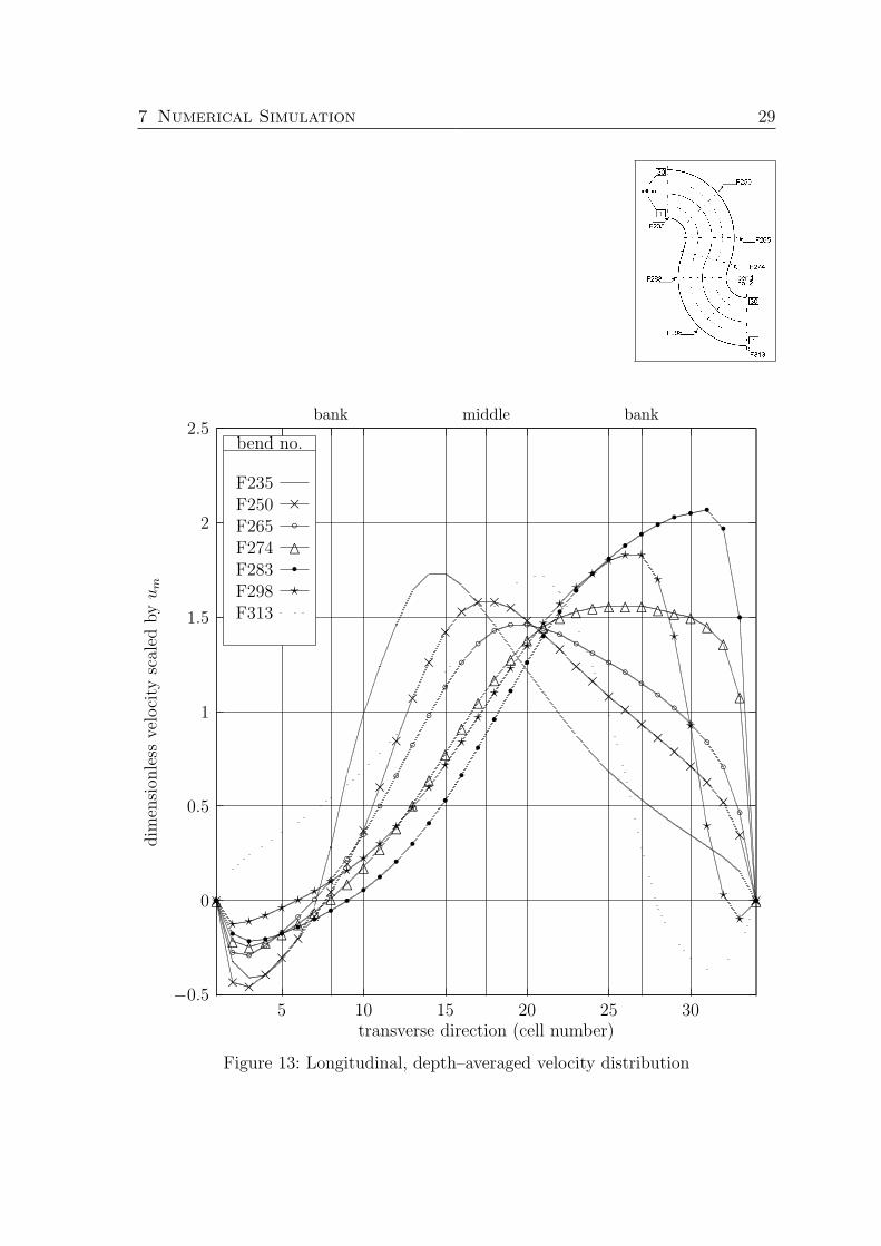
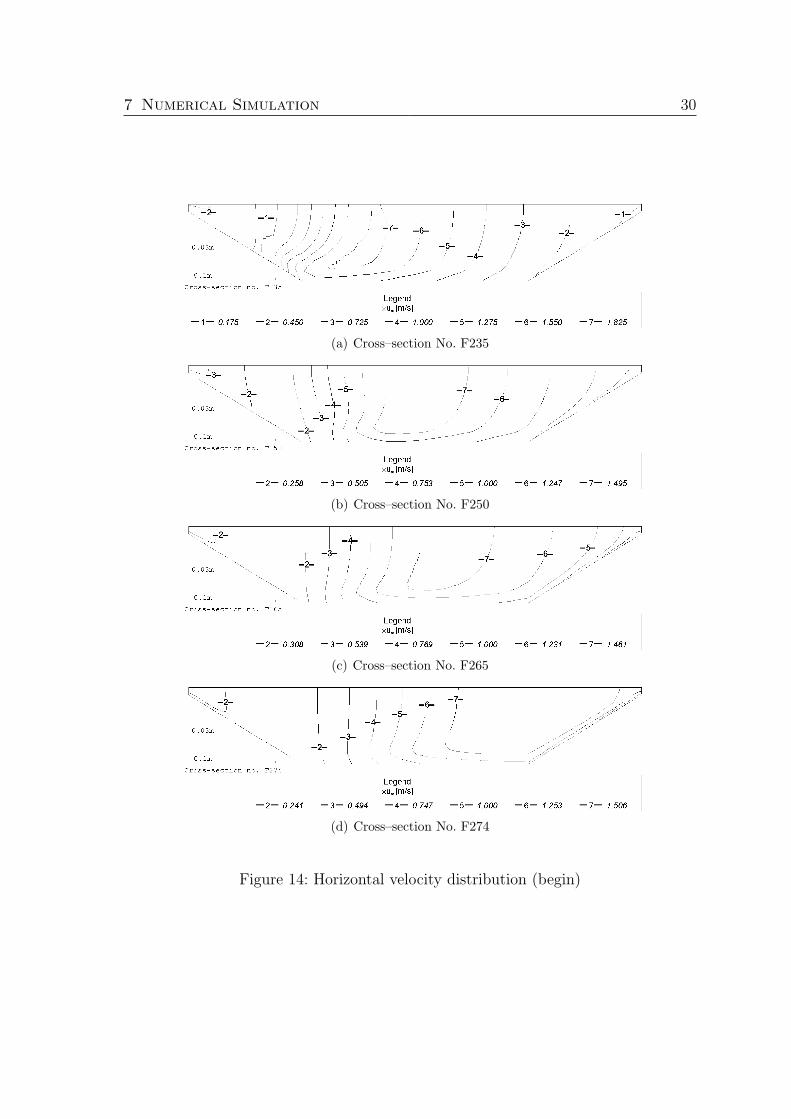
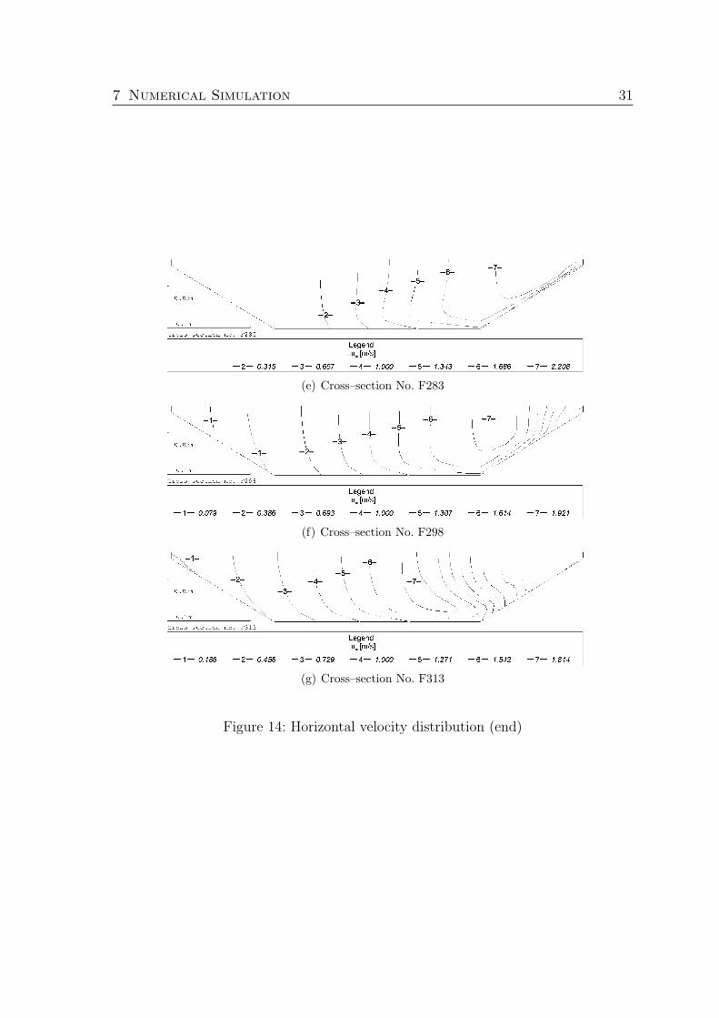
Besides the movement of the longitudinal velocity towards the concave bank, alsoa vertical movement of the maximum is observed. The cross-section at the apexesshows a longitudinal, depth–avaraged velocity maximum close to the middle of thecross-section, as described in chapter 7.2.3, but having a local peak at the bottom andthe beginning of sloping bed, as shown in Fig. 14(a). In this area the isotaches arecompressed, indicating strong velocity gradients. Considering the subsequent cross-sections, the core velocity moves towards the concave bank, while in the verticaldirection it drifts towards the center, as can be seen in Fig. 14(a) to Fig. 14(e). Thelines of equal velocity straighten out. Reaching the subsequent bend entrance, thebulk velocity moves to the convex bank, resulting in compressed isotaches and highvelocity gradients, where the whole bank area is affected (Fig. 14(e)). At the secondapex, the core velocity moves to the bottom again and the high velocity gradientsremain. Meckel [13] observed the same action.
7.2.5 Stream Separation and Formation of Recirculation Zone
No attention has been paid to the reverse velocities occurring at the convex banks.Rozovskii [21] states that in very acute bends there appears the phenomena of thestream being drawn away from the walls and of eddy zone formation.It is known that if the pressure along the flow increases, conditions arise for theseparation of the stream from the wall and for the appearance of eddy currents. Onthe other hand, where there is a positive gradient of pressure along the flow, thephenomena of separation is not observed. From Eulers equation, deceleration of fluidelements is caused by a negative pressure gradient. Stream separation is expected. Asmentioned in chapter 7.2.3, the bulk velocity moves towards the concave bank, wherethe fluid elements are accelerated. At the same time and for reason of conservation of
7 Numerical Simulation 29
−0.5
0
0.5
1
1.5
2
2.5
5 10 15 20 25 30
bank middle bank
dim
ensi
onle
ssve
loci
tysc
aled
by
um
transverse direction (cell number)
bend no.
F235F250
×
××××××××
×
×
×
×
×××××××
××××××××××××
×
×
×F265
bb b b b b b b b b b
bb b b b b b b b b b b b b b b b b b b b
b
b
bF274
M
M M M MM
MM
MM
MM
M
M
M
M
MM
MM
M M M M M M M M M M MM
M
M
MF283
rr r r r r r r r r r r r r r r r r r r r r r r r r r r r r r r
r
r
rF298
?
? ? ? ? ??
??
??
??
?
?
?
?
?
?
?
??
??
? ? ?
?
?
?
?
?
??
?
F313
Figure 13: Longitudinal, depth–averaged velocity distribution
7 Numerical Simulation 30
(a) Cross–section No. F235
(b) Cross–section No. F250
(c) Cross–section No. F265
(d) Cross–section No. F274
Figure 14: Horizontal velocity distribution (begin)
7 Numerical Simulation 31
(e) Cross–section No. F283
(f) Cross–section No. F298
(g) Cross–section No. F313
Figure 14: Horizontal velocity distribution (end)
7 Numerical Simulation 32
mass, the fluid elements at the convex bank are decelerated and a negative pressuregradient established, leading to a separation zone, expanding until the following apex.Rozovskii [21] found from experimental results that formation of separation zones areunlikely, even at sharp bends with a small ratio of center line curvature rc to widthB of rc/B = 1. In the investigated case the ratio equals rc/B = 0.916 < 1. To theextent that stream separation is connected to the negative acceleration effect of fluidelements at the side wall, Rozovskii [21] asserts that conditions for the appearanceof separation will also depend on the angle of bank slope. He concludes that thepossibility of separation increases, the gentler the bank slope is, or in short, the greaterthe influence of friction of the stream against the bank. As in the case consideredthe transverse bed slope angle equals α = 30 ◦, the calculated flow separation zone islikely, even in the case of a center line curvature radius to a width ratio close to one.
7.2.6 Concluding Remarks
Owing to a lack of measurement data, experimental verification for the water flowcalculation could not be obtained. Therefore, the absolute values of SSIIM resultspresented in this chapter can hardly be judged as right or wrong. Rather, the aimhere is limited to identifying a trend. The author must depend on experimental runsconducted and documented by researchers. The author has reviewed the literaturein order to verify the numerical results.
Since the flow pattern is sensitive to the presence of any preexisting circulation [2],only experiments with subsequent bends qualify for drawing comparisons.
The numerical calculation of SSIIM seems to qualitatively correspond to the resultsobtained in experiments by authors cited in this chapter, even considering differencesin geometry, roughness and flow parameters.
Proceeding from the assumption of physically correct numerical results, the waterflow calculation is the basis for the subsequent sediment transport calculation.
7.3 Presentation of Sediment Transport Results
The sediment transport simulation was carried out after having finished the calcula-tion of the water flow field as the initial condition. The basic sediment configuration,which will be referred to as the Base Case, is applied by the SSIIM program accord-ing to chapter 7.3.1. Roughness parameter, grid size as well as the time step arechanged afterwards. The results are analyzed in order to determine the sensitivityof the model to the specific changes and the capability of SSIIM to yield universallyvalid predictions.
7 Numerical Simulation 33
7.3.1 Basic Sediment Configuration
In the numerical simulation of sediment transport both bed–load and suspendedload transport must be considered as described in chapter 3.4. Applying a roughcalculation of the suspension parameter, Z is estimated to Z ≈ 13. From Fig. 4one can conclude that almost no sediment particles will be found in the water bodyabove the bed elements, if Z > 5. Furthermore, absence of suspended sedimentsduring the experimental run justifies the approximation of simulating the bed–loadtransport only. The SSIIM program is assigned to ignore the suspended load, havingthe positive effect of reducing computation time.
Several parameters must be passed to the SSIIM software and are kept constantin all presented numerical simulations, unless otherwise noted.The density of quartz minerals is typically ρs = 2650 kg/m3 and taken for calculation.Most natural sediments have densities similar to that of quartz. Another propertyof a sediment particle is its characteristic size d or D. The channel is formed inuniform sand of d50 = 0.7 mm diameter. The fall velocity in vertical direction of asediment particle is mostly important for suspended particle motion. van Rijn [25]assumes the bed–load particles are dominated by gravitational forces, while the effectof turbulence on the overall trajectory is supposed to be of minor importance. But hedoes not rule out particles jumping and leaving the bed surface for a short distanceand height. Therefore, the particle fall velocity must also be included even thoughbed–load is the major transport mode. The fall velocity is taken from Chanson [3,Table 7.3] to ws = 0.09 m/s and added to the second term on the left side of (2.10).The angle of repose φ must be specified as it is important for the incipient motion of aparticle as discussed in chapter 3.2. It depends on the grain size d, density ρs and itsdegree of saturation with water. In the vicinity of water a particle becomes unstable ascompared to a dry environment. Owing to buoyancy force, the density of a sedimentparticle is reduced to submerged sediment density. In the basic configuration theangle of repose is set to φ = 34.4 ◦.
The bed elevation changes over a time period because of erosion and/or deposition.The sediment calculation is transient and a time step ∂t has to be chosen. The timestep chosen must not be so large that changes in geometry cause the flow patternto change significantly. The shorter the time step ∂t, the more iterations have tobe calculated in order to carry out a simulation time of 4 h, which results in a longcomputation time. A time step of ∂t = 20 s is deemed to be a satisfactory compromisebetween numerical accuracy and computation time.
No sediment inflow is specified.
7.3.2 Default Case
A sediment transport calculation is carried out using the sediment transport approachof van Rijn [25] in conjunction with the standard computation of the dimensionless
7 Numerical Simulation 34
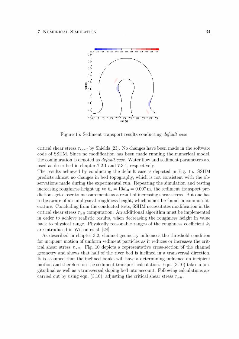
Figure 15: Sediment transport results conducting default case
critical shear stress τ∗,crit by Shields [23]. No changes have been made in the softwarecode of SSIIM. Since no modification has been made running the numerical model,the configuration is denoted as default case. Water flow and sediment parameters areused as described in chapter 7.2.1 and 7.3.1, respectively.The results achieved by conducting the default case is depicted in Fig. 15. SSIIMpredicts almost no changes in bed topography, which is not consistent with the ob-servations made during the experimental run. Repeating the simulation and testingincreasing roughness height up to ks = 10d50 = 0.007 m, the sediment transport pre-dictions get closer to measurements as a result of increasing shear stress. But one hasto be aware of an unphysical roughness height, which is not be found in common lit-erature. Concluding from the conducted tests, SSIIM necessitates modification in thecritical shear stress τcrit computation. An additional algorithm must be implementedin order to achieve realistic results, when decreasing the roughness height in valueback to physical range. Physically reasonable ranges of the roughness coefficient ks
are introduced in Wilson et al. [28].As described in chapter 3.2, channel geometry influences the threshold condition
for incipient motion of uniform sediment particles as it reduces or increases the crit-ical shear stress τcrit. Fig. 10 depicts a representative cross-section of the channelgeometry and shows that half of the river bed is inclined in a transversal direction.It is assumed that the inclined banks will have a determining influence on incipientmotion and therefore on the sediment transport calculation. Eqn. (3.10) takes a lon-gitudinal as well as a transversal sloping bed into account. Following calculations arecarried out by using eqn. (3.10), adjusting the critical shear stress τcrit.
7 Numerical Simulation 35
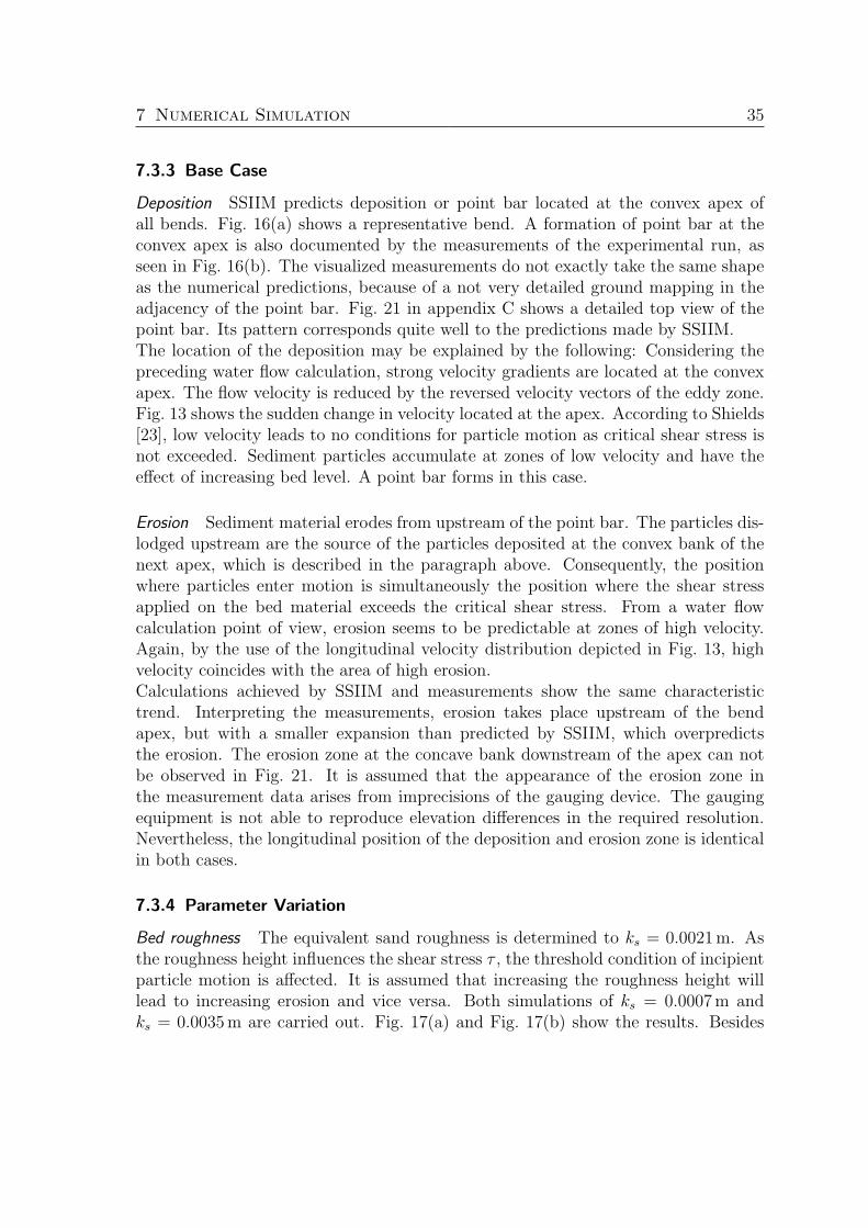
7.3.3 Base Case
Deposition SSIIM predicts deposition or point bar located at the convex apex ofall bends. Fig. 16(a) shows a representative bend. A formation of point bar at theconvex apex is also documented by the measurements of the experimental run, asseen in Fig. 16(b). The visualized measurements do not exactly take the same shapeas the numerical predictions, because of a not very detailed ground mapping in theadjacency of the point bar. Fig. 21 in appendix C shows a detailed top view of thepoint bar. Its pattern corresponds quite well to the predictions made by SSIIM.The location of the deposition may be explained by the following: Considering thepreceding water flow calculation, strong velocity gradients are located at the convexapex. The flow velocity is reduced by the reversed velocity vectors of the eddy zone.Fig. 13 shows the sudden change in velocity located at the apex. According to Shields[23], low velocity leads to no conditions for particle motion as critical shear stress isnot exceeded. Sediment particles accumulate at zones of low velocity and have theeffect of increasing bed level. A point bar forms in this case.
Erosion Sediment material erodes from upstream of the point bar. The particles dis-lodged upstream are the source of the particles deposited at the convex bank of thenext apex, which is described in the paragraph above. Consequently, the positionwhere particles enter motion is simultaneously the position where the shear stressapplied on the bed material exceeds the critical shear stress. From a water flowcalculation point of view, erosion seems to be predictable at zones of high velocity.Again, by the use of the longitudinal velocity distribution depicted in Fig. 13, highvelocity coincides with the area of high erosion.Calculations achieved by SSIIM and measurements show the same characteristictrend. Interpreting the measurements, erosion takes place upstream of the bendapex, but with a smaller expansion than predicted by SSIIM, which overpredictsthe erosion. The erosion zone at the concave bank downstream of the apex can notbe observed in Fig. 21. It is assumed that the appearance of the erosion zone inthe measurement data arises from imprecisions of the gauging device. The gaugingequipment is not able to reproduce elevation differences in the required resolution.Nevertheless, the longitudinal position of the deposition and erosion zone is identicalin both cases.
7.3.4 Parameter Variation
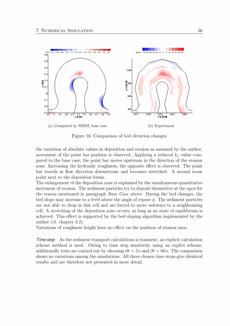
Bed roughness The equivalent sand roughness is determined to ks = 0.0021 m. Asthe roughness height influences the shear stress τ , the threshold condition of incipientparticle motion is affected. It is assumed that increasing the roughness height willlead to increasing erosion and vice versa. Both simulations of ks = 0.0007 m andks = 0.0035 m are carried out. Fig. 17(a) and Fig. 17(b) show the results. Besides
7 Numerical Simulation 36
(a) Computed by SSIIM, base case (b) Experiment
Figure 16: Comparison of bed elevation changes
the variation of absolute values in deposition and erosion as assumed by the author,movement of the point bar position is observed. Applying a reduced ks–value com-pared to the base case, the point bar moves upstream in the direction of the erosionzone. Increasing the hydraulic roughness, the opposite effect is observed. The pointbar travels in flow direction downstream and becomes stretched. A second scourpoint next to the deposition forms.The enlargement of the deposition zone is explained by the simultaneous quantitativeincrement of erosion. The sediment particles try to deposit themselves at the apex forthe reason mentioned in paragraph Base Case above. During the bed changes, thebed slope may increase to a level above the angle of repose φ. The sediment particlesare not able to drop in this cell and are forced to move sideways to a neighbouringcell. A stretching of the deposition zone occurs, as long as no state of equilibrium isachieved. This effect is supported by the bed sloping algorithm implemented by theauthor (cf. chapter 3.2).Variations of roughness height have no effect on the position of erosion area.
Time step As the sediment transport calculations is transient, an explicit calculationscheme method is used. Owing to time step sensitivity using an explict scheme,additionally tests are carried out by choosing ∂t = 5 s and ∂t = 60 s. The comparisonshows no variations among the simulations. All three chosen time steps give identicalresults and are therefore not presented in more detail.
7 Numerical Simulation 37
(a) ks = 0.0007m (b) ks = 0.0035m
Figure 17: Bed elevation changes with regard to different bed roughness heights
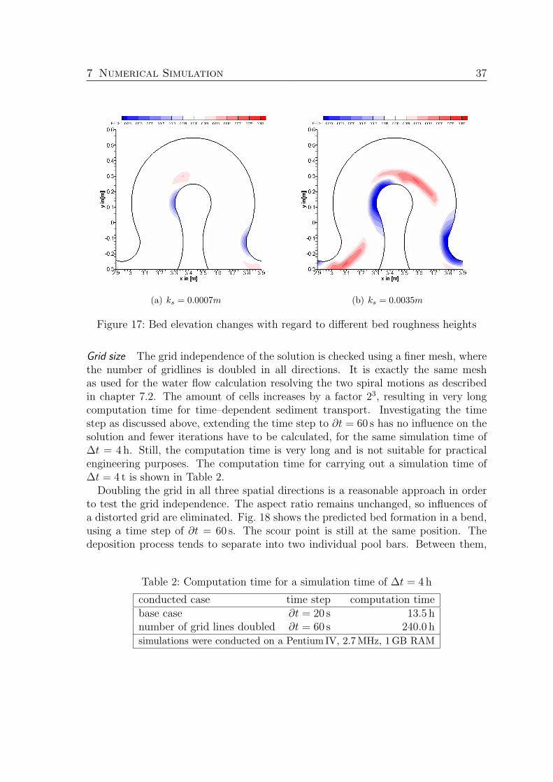
Grid size The grid independence of the solution is checked using a finer mesh, wherethe number of gridlines is doubled in all directions. It is exactly the same meshas used for the water flow calculation resolving the two spiral motions as describedin chapter 7.2. The amount of cells increases by a factor 23, resulting in very longcomputation time for time–dependent sediment transport. Investigating the timestep as discussed above, extending the time step to ∂t = 60 s has no influence on thesolution and fewer iterations have to be calculated, for the same simulation time of∆t = 4 h. Still, the computation time is very long and is not suitable for practicalengineering purposes. The computation time for carrying out a simulation time of∆t = 4 t is shown in Table 2.
Doubling the grid in all three spatial directions is a reasonable approach in orderto test the grid independence. The aspect ratio remains unchanged, so influences ofa distorted grid are eliminated. Fig. 18 shows the predicted bed formation in a bend,using a time step of ∂t = 60 s. The scour point is still at the same position. Thedeposition process tends to separate into two individual pool bars. Between them,
Table 2: Computation time for a simulation time of ∆t = 4 h
conducted case time step computation timebase case ∂t = 20 s 13.5 hnumber of grid lines doubled ∂t = 60 s 240.0 hsimulations were conducted on a Pentium IV, 2.7 MHz, 1 GB RAM
7 Numerical Simulation 38
Figure 18: Sediment calculation with refined mesh and ∂t = 60s
a scour point develops. Comparing the numerical result to another photo taken ofa bend during the experimental run, similarities are observed. At a different benda different bed formation pattern appears as presented in Fig. 22. To gather fromthis observation, neither the experimental run nor the numerical simulation seemsto tend to a prefered solution. The predictions show variations in detail, but themain characteristic, which is the formation of a pool bar at the convex apex, remainsunchanged.
Wilson et al. [28] conducts numerical water flow simulations of a pseudo–naturalmeandering flow, using a distorted computation mesh in a longitudinal direction.To check if the result is mesh independent, a simulation is conducted using a meshwith double the number of gridlines in a longitudinal direction, making the mesh lessdistorted. The computed velocities from the two grids were found to be reasonably inagreement. Mesh independence is confirmed and even a distorted mesh gives accurateresults.Also a distorted mesh was tested for sediment transport calculations in this study.Therefore, the number of grid cells in only the transversal and vertical direction wasdoubled. Simulations having a time step of ∂t = 20 s and ∂t = 60 s were carried out.The sediment calculation results are presented in Fig. 19. Considering a time step of∂t = 60 s of the fine mesh calculation and comparing the results achieved by a finebut distorted mesh, the bed formation pattern is quite similar. This observation leadsto the conclusion that the accuracy of the solution is not affected by a refinement ofthe grid in a longitudinal direction.
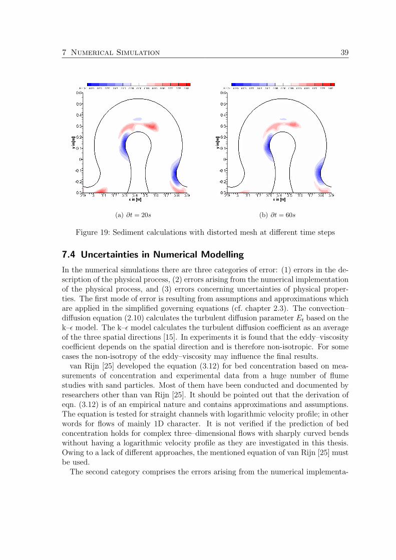
7 Numerical Simulation 39
(a) ∂t = 20s (b) ∂t = 60s
Figure 19: Sediment calculations with distorted mesh at different time steps
7.4 Uncertainties in Numerical Modelling
In the numerical simulations there are three categories of error: (1) errors in the de-scription of the physical process, (2) errors arising from the numerical implementationof the physical process, and (3) errors concerning uncertainties of physical proper-ties. The first mode of error is resulting from assumptions and approximations whichare applied in the simplified governing equations (cf. chapter 2.3). The convection–diffusion equation (2.10) calculates the turbulent diffusion parameter Et based on thek–ε model. The k–ε model calculates the turbulent diffusion coefficient as an averageof the three spatial directions [15]. In experiments it is found that the eddy–viscositycoefficient depends on the spatial direction and is therefore non-isotropic. For somecases the non-isotropy of the eddy–viscosity may influence the final results.
van Rijn [25] developed the equation (3.12) for bed concentration based on mea-surements of concentration and experimental data from a huge number of flumestudies with sand particles. Most of them have been conducted and documented byresearchers other than van Rijn [25]. It should be pointed out that the derivation ofeqn. (3.12) is of an empirical nature and contains approximations and assumptions.The equation is tested for straight channels with logarithmic velocity profile; in otherwords for flows of mainly 1D character. It is not verified if the prediction of bedconcentration holds for complex three–dimensional flows with sharply curved bendswithout having a logarithmic velocity profile as they are investigated in this thesis.Owing to a lack of different approaches, the mentioned equation of van Rijn [25] mustbe used.
The second category comprises the errors arising from the numerical implementa-
7 Numerical Simulation 40
tion of the physical processes, e.g. false diffusion generated by the numerical grid ornon-orthogonal diffusive terms, which are neglected for the calculation of the sedi-ment concentrations. An injudicious parameter choice can produce highly erroneousresults, even if remaining parameters are set correctly. On the other hand, a reason-able diligence in the model establishment by the user may minimize these errors.The remedy to prevent false diffusion is to align the grid with the fluid directionand/or increase the number of elements in the grid [15]. The author has tested thesecond approach. As described in chapter 7.3.4, doubling the number of cells in eachdirection does not change the accuracy of the solution. Consequently, inaccuracy isnot caused by false diffusion. Another alternative is to use a second-order method asapplied throughout all simulations.
The third category of error mentioned concerns the uncertainty of physical prop-erties, e.g. roughness height and angle of repose φ. The latter is set to a constantvalue as recommended by the literature for submerged sand particles. During theexperimental runs, φ varies with time. At the beginning of the experiment the sandis dry and becomes saturated with water gradually. The variation of φ during theexperiment is time-dependent and is not reproduceable in SSIIM.Special attention is paid to the equivalent sand roughness coefficient ks as it influencesthe bed friction and therefore the bed–load transport. In the numerical simulation,the ks–value is adjusted until the model output matches the measured conditionsby the experiment. This is achieved using an equivalent sand roughness height ofks = 0.0021 m, which corresponds to ks = 2.3d90, if d90 = 0.0009 m as seen in Fig. 8.The value found from this calibration is in the range of empirically found values pre-sented by Wilson et al. [28].Fig. 16(a) shows an overprediction in erosion by the SSIIM software. The sedimentmaterial located at the convex bank is carried away by current force. The photosshown in Fig. 21 and Fig. 22 taken from the bend do not exhibit such strong erosion,but rather demonstrate resistance to the acting force. Speculating about this observa-tion, the sediment particles could exercise cohesion forces and stick together, havingthe effect of variation in threshold condition for incipient sediment motion. Besidesthis explanation, there could also be a compaction of the sediment material duringthe formation of the trapezoidal shape. The mentioned influences are very uncertainand almost impossible to quantify or to consider in the numerical simulation.
8 Conclusions and Outlook
This thesis presents a comparison of simulations performed in the numerical modelSSIIM and a physical model. The objective is to examine the modelling resultswith respect to the sediment processes observed in the experimental run in order todetermine whether or not the numerical model SSIIM is able to predict sedimenttransport correctly.
The physical process of sediment transport and its implementation in the numericalmodel was described. Furthermore, the software code was extended by a subroutinetaking generalized sloping bed for incipient particle motion into account [5]. The sub-routine emerges as the key for achieving improved results, reproducing the sedimentprocesses as closely as possible to the experiment.
Influencing factors are the calibration coefficients, i.e. the equivalent sand rough-ness height. Suggestions from the literature were adopted, but further simulationshave shown that small variations in roughness will strongly effect the bed formationpattern. The time step variation shows minor change, so that this parameter shouldnot be taken as a calibration coefficient of the numerical model. The degree of itsinfluence on the results in combination with changes in grid size could be an interest-ing topic for further studies. But due to long computation times, such investigationscan not be carried out in a reasonable time with present computer capacity.
The numerical model results have proved to be grid size independent in combinationwith the time steps chosen by the author. A refined grid shows separation of the pointbar, reflecting observations documented by photos but not by measurements.
The software SSIIM performs capably in reproducing sediment transport processesin a realistic way, even with regard to sharply curved bends. The calculation can becarried out if the user establishes reasonable model assumptions and approximations.In this thesis, results in good agreement to the experiment have been achieved evenwith the coarsest grid tested and a time step of ∂t = 60 s for a simulation timeof ∆t = 4 t. The computation time is as long as it is appropriate for practicalengineering purpose. Refining the computational mesh or decreasing the time stepmeans extending computation time, which is not feasible with the power of present–day personal computers (cf. Table 2). Conducted calculations concerning variationof the mentioned numerical parameters do not yield any improvement of the resultaccuracy. They show variations of the bed formation pattern as also observed inthe experiment. However, without having field data, running reliable simulations ishardly not possible. But even if applying unphysical parameters, SSIIM is able toindicate the trend of pool- resp. point bar formation.
SSIIM’s extension by the implemented subroutine shows that the software is a re-liable instrument in river, environmental and sedimentation engineering. The abilityto run the software on standard personal computers will promote its distributionamong practical working hydraulic engineers and will cause it to be accepted as adesign tool for water and environmental related engineering.
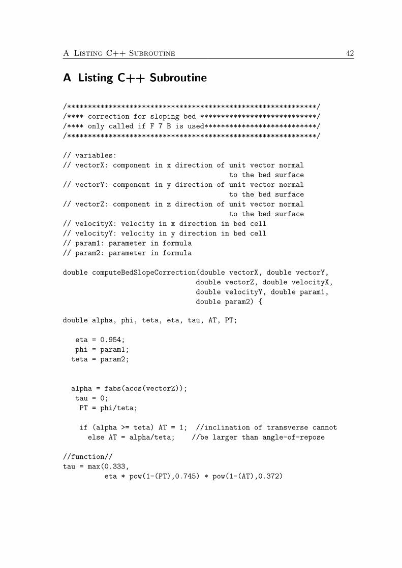
A Listing C++ Subroutine 42
A Listing C++ Subroutine
/************************************************************/
/**** correction for sloping bed ****************************/
/**** only called if F 7 B is used***************************/
/************************************************************/
// variables:
// vectorX: component in x direction of unit vector normal
to the bed surface
// vectorY: component in y direction of unit vector normal
to the bed surface
// vectorZ: component in z direction of unit vector normal
to the bed surface
// velocityX: velocity in x direction in bed cell
// velocityY: velocity in y direction in bed cell
// param1: parameter in formula
// param2: parameter in formula
double computeBedSlopeCorrection(double vectorX, double vectorY,
double vectorZ, double velocityX,
double velocityY, double param1,
double param2) {
double alpha, phi, teta, eta, tau, AT, PT;
eta = 0.954;
phi = param1;
teta = param2;
alpha = fabs(acos(vectorZ));
tau = 0;
PT = phi/teta;
if (alpha >= teta) AT = 1; //inclination of transverse cannot
else AT = alpha/teta; //be larger than angle-of-repose
//function//
tau = max(0.333,
eta * pow(1-(PT),0.745) * pow(1-(AT),0.372)

A Listing C++ Subroutine 43
); //max, barrier for alpha-->teta
return tau;}
//************ from Joern ****************//
B Listing of Sediment Calculation Input File 44
B Listing of Sediment Calculation Input File
T sed_shf_.21mm_20s_NNN_9degree title field
F 1 CD
F 2 RIS run option (result, initialize, sediment)
F 4 0.5 50 0.001 concentration calculation, relaxation,
iterations, convergence
F 7 B correction sloping bed
F 11 2.65 -0.03 density and shield coefficient
F 16 0.0021 roughness coef. of walls and bed
F 33 20.0 100 time step 20sec, inner iterations
F 37 1 tcs algorith
F 48 9 tecplot option
F 54 0.001 residual during transient calculation convergence criteria
F 56 10 0.5 number iterations, angle of response
f 78 1 0.0 sediments not follow flow vectors
F 84 1 v rijn bed load formular
F 109 5.368e-04 0.6 0.0 bed slope phi teta 0.0
F 111 1 beddll.dll
F 155 2.0 0 different sediment distribution at banks
G 1 261 17 9 1 grid and array sizes
G 3 0.000 12.5 25.00 37.5 50.0 62.50 75.00 87.50 100.00
vertical grid distribution
G 7 0 1 2 17 2 9 0 0 0.001 1 0 0.0 inflow
G 7 1 -1 2 17 2 9 0 0 0.001 1 0 0 outflow
P 10 1 number of iterations between printing results tecplot
S 1 0.0007 0.09 sediments_size and fall velocity
N 0 1 1 composition of sieve line
I 1 0.00 sediment inflow kg/s
B 0 0 0 0 0 spatial distribution of sediment
W 1 34.15 0.001 0.04397 kst, discharge, downstream water level
W 2 8 1 40 80 120 160 200 240 261 backwater calculation
K 1 720 60000 iteration options 4hours
B Listing of Sediment Calculation Input File 45
K 2 0 1 sidewall/surface 0=wall law/1=free surface
K 3 0.8 0.8 0.8 0.3 0.5 0.5 relaxation factors
K 6 1 1 1 0 0 0 1-->2nd order up-w.scheme, u,v,w,p,k,e
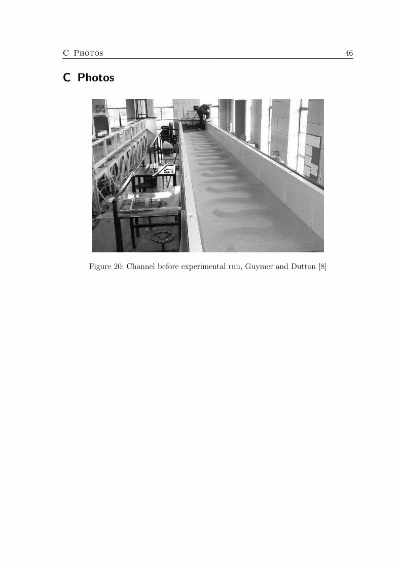
C Photos 46
C Photos
Figure 20: Channel before experimental run, Guymer and Dutton [8]
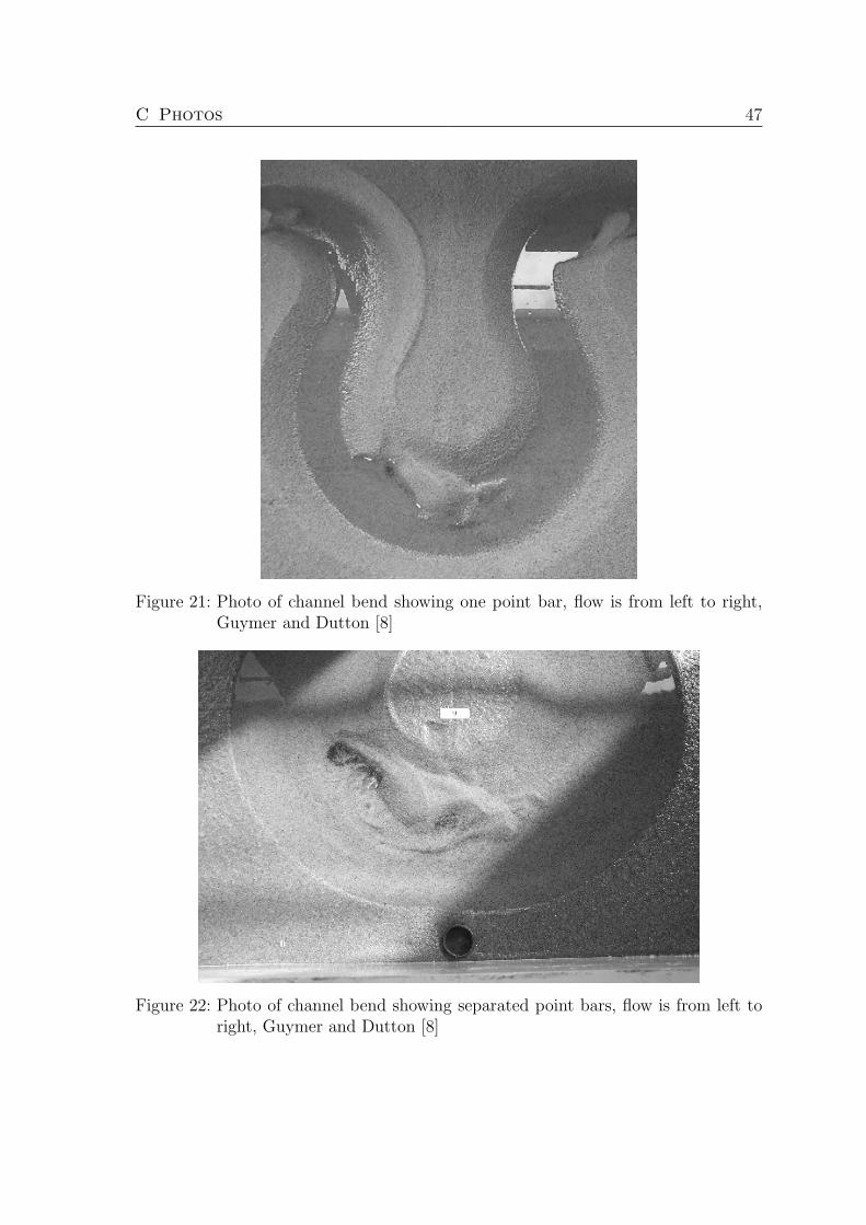
C Photos 47
Figure 21: Photo of channel bend showing one point bar, flow is from left to right,Guymer and Dutton [8]
Figure 22: Photo of channel bend showing separated point bars, flow is from left toright, Guymer and Dutton [8]
References 48
References
[1] Wasser- und Schifffahrtsamt Freiburg. Information Flyer, 2004.
[2] Bathurst, James C., Thorne, Colin R., and Hey, Richard D. Secondary flow andshear stress at river bends. Journal of the Hydraulics Division, 10:1277–1295,October 1979.
[3] Chanson, Hubert. The Hydraulics of Open Channel Flow: An Introduction. El-sevier Butterworth–Heinemann, Amsterdam, Bosten, Heidelberg, London, NewYork, Oxford, 2 edition, 2004. ISBN 0–7506–5978–5.
[4] Ciray, Cahit. On secondary currents. The International Association for Hy-draulic Research, 1:408–413, September 1967. 12th IAHR–Congress, FortCollins, 11–14. September 1967.
[5] Dey, Subhasish. Experimental study on incipient motion of sediment particleson generalized sloping fluvial beds. International Journal of Sediment Research,16:391–398, 2001. No. 3.
[6] Dey, Subhasish. Threshold of sediment motion on combined transverse andlongitudinal sloping beds. Journal of Hydraulic Research, 41:405–415, 2003.No. 4.
[7] Fischer, Hugo B., List, E. John, Koh, Robert C. Y., Imberger, Joerg, and Brooks,Norman H. Mixing in Inland and Coastal Waters. Academic Press, New York,London, Toronto, Sydney, San Francisco, 1979. ISBN 0-12-258150-4.
[8] Guymer, Ian and Dutton, Richard. Measurement data and photographs of phys-ical experiment. unpublished, 2003. kindly left to the author.
[9] Imiela, Manfred. Langfristige mehrdimensionale Feststofftransportmodellierungzum morphologischen Gleichgewichtszustand anhand von Modellversuchen undeiner Renaturierungsmaßnahme an der Enz. Master’s thesis, Universitat Karls-ruhe, 2004. Institut fur Hydromechanik.
[10] Julien, Pierre Y. Erosion and Sedimentation. Cambridge University Press, Cam-bridge, United Kingdom, 1989. ISBN 0–521–63639–6.
[11] Kobus, Helmut. Wasserbauliches Versuchswesen, volume 4. DVWW, Essen,1978. Mitteilungsheft.
[12] Leschziner, Michael A. and Rodi, Wolfgang. Calculation of strongly curved openchannel flow. Journal of the Hydraulics Division, 10:1297–1314, October 1979.
References 49
[13] Meckel, Hermann. Spiralstromung und Sedimentbewegung in Fluss– undKanalkrummungen. Wasserwirtschaft, 10:287–294, Oktober 1978. Heft 10.
[14] Mosonyi, Emil and Gotz, Werner. Secondary currents in subsequent modelbends. International Symposium on River Mechanics, 1:191–201, January 1973.Proceedings of the International Association for Hydraulic Research, 9–12 Jan-uary 1973, Asian Institute of Technology, Bangkok, Thailand.
[15] Olsen, Nils Reidar B. A three-dimensional numerical model for simulation ofsediment movements in water intakes. PhD thesis, Division of Hydraulic En-gineering, University of Trondheim, Norwegian Institute of Technology, 1991.59.
[16] Olsen, Nils Reidar B. A Three–Dimensional Numerical Model for Simulationof Sediment Movements in Water Intakes with Multiblock Option. Departmentof Hydraulic and Environmental Engineering, The Norwegian University of Sci-ence and Technology, 2002. URL http://www.ntnu.no/~nilsol/ssiimwin/
manual3.pdf. user’s manual.
[17] Patankar, Suhas V. Numerical heat transfer and fluid flow. HemispherePubl. Corp., New York, 1980. ISBN 0-89116-522-3.
[18] Prandtl, Ludwig, Oswatitsch, Klaus, and Wieghardt, Karl. Fuhrer durch dieStromungslehre. Friedr. Vieweg & Sohn, Braunschweig, Wiesbaden, 1984. ISBN3–528-18209–5. 8. vollstandig uberarbeitete Auflage.
[19] Rodi, Wolfgang. Turbulence Models and Their Application in Hydraulics. Inter-national Association for Hydraulics Research, Balkema, Rotterdam, 3rd edition,1993. ISBN 90 5410 150 4. A state–of–the–art review.
[20] Rouse, Hunter. Hydraulics, Mechanics of Fluids, Engineering Education, pages57–61. Selected Writings of Hunter Rouse. Dover Publications, Inc., New York.Institute of Hydraulic Research, University of Iowa.
[21] Rozovskii, I. L. Flow of Water in Bends of Open Channels, volume PST Cat.No. 363. Academy of Sciences of the Ukrainian SSR, Kiev, 1957. translation byY. Prushansky, Israel Program for Scientific Translation, 1961.
[22] Schlichting, Herrmann and Gersten, Klaus. Boundary Layer Theory. SpringerVerlag, Berlin, Heidelberg, New York, 8th revised and enlarged edition, 2000.ISBN 3-540-66270-7.
[23] Shields, Albert. Anwendung der Ahnlichkeitsmechanik und der Turbulenz-forschung auf die Geschiebebewegung. Mitteilungen der Preußischen Versuch-sanstalt fur Wasserbau und Schiffbau, 26:26, 1936. (in German).
[24] Socolofsky, Scott A. and Jirka, Gerhard H. Environmental Fluid MechanicsPart I, Mass Transfer and Diffusion. Class notes, 2002. Institut for Hydrome-chanics, University of Karlsruhe.
[25] van Rijn, Leo C. Sediment Transport, Part I: Bed Load Transport. Journalof Hydraulic Engineering, American Society of Civil Engineers, 110:1431–1456,October 1984. No. 10.
[26] van Rijn, Leo C. Sediment Transport, Part II: Suspended Load Transport.Journal of Hydraulic Engineering, American Society of Civil Engineers, 110:1613–1641, November 1984. No. 11.
[27] van Rijn, Leo C. Sediment Transport, Part III: Bed Forms and Alluvial Rough-ness. Journal of Hydraulic Engineering, American Society of Civil Engineers,110:1733–1755, December 1984. No. 12.
[28] Wilson, C.A.M.E., Boxall, J.B., Guymer, I., and Olsen, N.R.B. Validation of athree–dimensional numerical code in the simulation of pseudo–natural meander-ing flows. Journal of the Hydraulic Engineering, 10:758–768, October 2003.
[29] Zanke, Ulrich. Grundlagen der Sedimentbewegung. Springer Verlag, Berlin, Hei-delberg, New York, 1982. ISBN 3–540–11672–9.