applied bayesian inference - kit · 1 introduction 1.1 course overview computing i r – mostly...
TRANSCRIPT

Applied Bayesian Inference
Prof. Dr. Renate Meyer1,2
1Institute for Stochastics, Karlsruhe Institute of Technology, Germany2Department of Statistics, University of Auckland, New Zealand
KIT, Winter Semester 2010/2011
Prof. Dr. Renate Meyer Applied Bayesian Inference 1 Prof. Dr. Renate Meyer Applied Bayesian Inference 2
1 Introduction 1.1 Course Overview
Overview: Applied Bayesian Inference A
I Bayes theorem, discrete – continuousI Conjugate examples: Binomial, ExponentialI Introduction to RI Simulation-based posterior computationI Introduction to WinBUGSI Regression, ANOVA, GLM, hierarchical models, survival analysis,
state-space models for time series, copulasI Basic model checking with WinBUGSI Convergence diagnostics with CODA
Prof. Dr. Renate Meyer Applied Bayesian Inference 3
1 Introduction 1.1 Course Overview
Overview: Applied Bayesian Inference B
I Conjugate examples: Poisson, Normal, Exponential FamilyI Specification of prior distributionsI Likelihood PrincipleI Multivariate and hierarchical modelsI Techniques for posterior computationI Normal approximationI Non-iterative SimulationI Markov Chain Monte CarloI Bayes Factors, model checking and determinationI Decision-theoretic foundations of Bayesian inference
Prof. Dr. Renate Meyer Applied Bayesian Inference 4

1 Introduction 1.1 Course Overview
Computing
I R – mostly covered in classI WinBUGS – completely covered in classI Other – at your own risk
Prof. Dr. Renate Meyer Applied Bayesian Inference 5
1 Introduction 1.2 Why Bayesian Inference?
Why Bayesian Inference?
Or: What is wrong with standard statistical inference?
The two mainstays of standard/classical statistical inference areI confidence intervals andI hypothesis tests.
Anything wrong with them?
Prof. Dr. Renate Meyer Applied Bayesian Inference 6
1 Introduction 1.2 Why Bayesian Inference?
Example: Newcomb’s Speed of Light
Example 1.1Light travels fast, but it is not transmitted instantaneously. Light takesover a second to reach us from the moon and over 10 billion years toreach us from the most distant objects yet observed in the expandinguniverse. Because radio and radar also travel at the speed of light, anaccurate value for that speed is important in communicating withastronauts and orbiting satellites. An accurate value for the speed oflight is also important to computer designers because electrical signalstravel only at light speed.The first reasonably accurate measurements of the speed of light weremade by Simon Newcomb between July and September 1882. Hemeasured the time in seconds that a light signal took to pass from hislaboratory on the Potomac River to a mirror at the base of theWashington Monument and back, a total distance of 7400m. His firstmeasurement was 24.828 millions of a second.
Prof. Dr. Renate Meyer Applied Bayesian Inference 7
1 Introduction 1.2 Why Bayesian Inference?
Newcomb’s Speed of Light: CI
Let us assume that the individual measurementsXi ∼ N(µ, σ2 = 0.0052) with known measurement varianceσ2 = 0.0052. We want to find a 95% confidence interval for µ.
Answer: x ± 1.96× σ/√
n
Because asX − µσ/√
n∼ N(0,1):
P(−1.96 <
X − µσ/√
n< 1.96
)= 0.95
P(X − 1.96σ/
√n < µ < X − 1.96σ/
√n)
= 0.95P(24.8182 < µ < 24.8378) = 0.95
This means that µ is in this interval with 95% probability.Certainly NOT!Prof. Dr. Renate Meyer Applied Bayesian Inference 8

1 Introduction 1.2 Why Bayesian Inference?
Newcomb’s Speed of Light: CI
After collecting the data and computing the CI, this interval eithercontains the true mean or it does not. Its coverage probability is not0.95 but either 0 or 1.
Then where does our 95% confidence come from?
Let us do an experiment:I draw 1000 samples of size 10 each from N(24.828,0.0052)
I for each sample calculate the 95% CII check whether the true µ = 24.828 is inside or outside the CI
Prof. Dr. Renate Meyer Applied Bayesian Inference 9
1 Introduction 1.2 Why Bayesian Inference?
Newcomb’s Speed of Light: Simulation
S1
Coverage to dateSample
90.0%10th
88.9%
100%
100%
100%
100%
100%
100%
9th
8th
7th
6th
5th
4th
3rd
100%2nd
100%1st
94.0%100th
……. …….
The Level of ConfidenceTrue mean
95.2%991st……. …….
95.2%1000th……. …….
24.8
Figure 1: Coverage over repeated sampling.
Prof. Dr. Renate Meyer Applied Bayesian Inference 10
1 Introduction 1.2 Why Bayesian Inference?
Newcomb’s Speed of Light: CI
I 952 of the 1000 CIs include the true mean.I 48 of the 1000 CIs do not include the true mean.I In reality, we don’t know the true mean.I We do not sample repeatedly, we only take one sample and
calculate one CI.I Will this CI contain the true value?I It either will or will not but we do not know.I We take comfort in the fact that the method works 95% of the time
in the long run, i.e. the method produces a CI that contains theunknown mean 95% of the time that the method is used in thelong run.
Prof. Dr. Renate Meyer Applied Bayesian Inference 11
1 Introduction 1.2 Why Bayesian Inference?
Newcomb’s Speed of Light: CI
By contrast, Bayesian confidence intervals, known as credible intervalsdo not require this awkward frequentist interpretation.
One can make the more natural and direct statement concerning theprobability of the unknown parameter falling in this interval.
One needs to provide additional structure to make this interpretationpossible.
Prof. Dr. Renate Meyer Applied Bayesian Inference 12

1 Introduction 1.2 Why Bayesian Inference?
Newcomb’s Speed of Light: Hypothesis Test
H0 : µ ≤ µ0(= 24.828) versus H1 : µ > µ0
I Test statistic:
U =X − µ0
σ/√
n∼ N(0,1) if µ = µ0
I Small values of uobs are consistent with H0, large values favour H1
I P-value:p = P(U > uobs|µ = µ0) = 1− Φ(u0)
I if P-value < 0.05 (= usual type I error rate), reject H0
The P-value is the probability that H0 is true.Certainly NOT.
Prof. Dr. Renate Meyer Applied Bayesian Inference 13
1 Introduction 1.2 Why Bayesian Inference?
Newcomb’s Speed of Light: Hypothesis Test
The P-value is the probability to observe a value of the test statisticthat is more extreme than the actually observed value uobs if the nullhypothesis were true (under repeated sampling).
We can do another thought experimentI imagine we take 1000 samples of size 10 from a Normal
distribution with mean µ0.I we calculate the P-value for each sample.I it will only we smaller than 0.05 in about 5% of the samples, in
about 50 samples.I we take comfort in the fact that this test works 95% of the time in
the long run, i.e. rejects H0 even though H0 is true only in 5% ofthe cases that this method is used.
Prof. Dr. Renate Meyer Applied Bayesian Inference 14
1 Introduction 1.2 Why Bayesian Inference?
Newcomb’s Speed of Light: Hypothesis Test
I It can only offer evidence against the null hypothesis. A largeP-value does not offer evidence that H0 is true.
I P-value cannot be directly interpreted as "weight of evidence" butonly as a long-term probability (in a hypothetical repetition of thesame experiment) of obtaining data at least as unusual as whatwas actually observed.
I Most practitioners are tempted to say that the P-value is theprobability that H0 ist true.
I P-values depend not only on the observed data but also thesampling probability of certain unobserved datapoints. Thisviolates the Likelihood Principle.
I This has serious practical implications for instance for the analysisof clinical trials, where often interim analyses and unexpecteddrug toxicities change the original trial design.
Prof. Dr. Renate Meyer Applied Bayesian Inference 15
1 Introduction 1.2 Why Bayesian Inference?
Newcomb’s Speed of Light: Hypothesis Test
By contrast, the Bayesian approach to hypothesis testing, dueprimarily to Jeffreys (1961) is much simpler and avoids the pitfalls ofthe traditional Neyman-Pearson-based approach.
It allows the direct calculation of the probability that a hypothesis istrue and thus a direct and straightforward interpretation.
Again, as in the case of CIs, we need to add more structure to theunderlying probability model.
Prof. Dr. Renate Meyer Applied Bayesian Inference 16

1 Introduction 1.3 Historical Overview
Historical Overview
Figure 2: From William Jefferys’ webpage, Univ. of Texas at Austin.
Prof. Dr. Renate Meyer Applied Bayesian Inference 17
1 Introduction 1.3 Historical Overview
Inverse Probability
I Bayes and Laplace (late 1700’s) – inverse probabilityI Example: Given x successes in n iid trials with success probabilityθ
I probability – statements about observables given assumptionsabout unknown parameters
P(9 ≤ X ≤ 12|θ)
deductive
I inverse probability – statements about unknown parameters givenobserved data values
P(a < θ < b|X = 9)
inductive
Prof. Dr. Renate Meyer Applied Bayesian Inference 18
1 Introduction 1.3 Historical Overview
Thomas Bayes
(b. 1702, London – d. 1761, Tunbridge Wells, Kent)
Bellhouse, D.R. (2004) The Reverend Thomas Bayes: FRS: ABiography to Celebrate the Tercentenary of His Birth. StatisticalScience 19(1):3-43.
Figure 3: Reverend Thomas Bayes 1702-1761.
Prof. Dr. Renate Meyer Applied Bayesian Inference 19
1 Introduction 1.3 Historical Overview
Bayes’ Biography
Presbyterian minister and mathematician
Son of one of the first 6 Nonconformist ministers in England
Private education (by De Moivre?)
Ordained as Nonconformist minister and took the position as ministerat the Presbyterian Chapel, Tunbridge Wells
Educated and interested in mathematics, probability and statistics,believed to be the first to use probability inductively, defended theviews and philosophy of Sir Isaac Newton against criticism by BishopBerkeley
Two papers published while he was still living:I Divine Providence and Government is the Happiness of His
Creatures (1731)I An Introduction to the Doctrine of Fluxions, and a Defense of the
Analyst (1736)Prof. Dr. Renate Meyer Applied Bayesian Inference 20

1 Introduction 1.3 Historical Overview
Bayes’ Biography
Elected Fellow of the Royal Society in 1742Most well-known paper published posthumously, submitted by hisfriend Richard Price,”Essay Towards Solving a Problem in the Doctrine of Chances" (1763),Philosophical Trans. of the Royal Society of Londonbegins with :
Given the number of times in which an unknown eventhas happened and failed: Required the chance that theprobability of its happening in a single trial liessomewhere between any two degrees of probability thatcan be named.
Prof. Dr. Renate Meyer Applied Bayesian Inference 21
1 Introduction 1.3 Historical Overview
Bayes’ Biography
Figure 4: Bayes’ vault at Bunhill Fields, London
Prof. Dr. Renate Meyer Applied Bayesian Inference 22
1 Introduction 1.3 Historical Overview
18 and 19th Century
Bayes laid the foundations of modern Bayesian statistics
Pierre Simon Laplace (1749-1827), French mathematician andastronomer, developed mathematical astronomy and statisticsrefined inverse probablity, acknowledging Bayes’ work in a monographin 1812
George Boole challenged inverse probability in his Laws of Thought in1854. The Bayesian approach has been controversial ever since butwas predominent in practical applications until the early 20th centurybecause of a lack of a frequentist alternative. Inverse probabilitybecame an integral part of the Universities’ statistics curriculum.
Prof. Dr. Renate Meyer Applied Bayesian Inference 23
1 Introduction 1.3 Historical Overview
20th Century
Sir R.A. Fisher (1890-1962) was a lifelong critic of inverse probability.and one of the most important persons involved in the demise ofinverse probability.
Figure 5: Sir Ronald A. Fisher (1890-1962) .Prof. Dr. Renate Meyer Applied Bayesian Inference 24

1 Introduction 1.3 Historical Overview
20th Century
Fisher’s (1922) paper revolutionized statistical thinking by introducingthe notions of "maximum likelihood", "sufficiency", and "efficiency". Hismain argument was that one needed to look at the likelihood of thedata given the theory NOT the likelihood of the theory given the data.He thus advocated an "indirect" approach to statistical inference basedon ideas of logic called "proof by contradiction".His work impressed two young statisticians at University CollegeLondon: J. Neyman and E. Pearson. They developed the mathematicaltheory of significance testing and confidence intervals which had ahuge influence on statistical applications (for good or bad).
Prof. Dr. Renate Meyer Applied Bayesian Inference 25
1 Introduction 1.3 Historical Overview
Rise of Subjective Probability
Inverse probability ideas were studied by Keynes (1921), Borel (1921)and Ramsay (1926).In 1930’s Harold Jeffreys engaged in a published exchange with R.A.Fisher on Fisher’s fiducial argument and Jeffreys’ inverse probability.Jeffreys’ (1939) book on "Theory of Probability" is the most cited in thecurrent "objective Bayesian" literature.In Italy in the 1930s, Bruno de Finetti gave a different justification forsubjective probability, introducing the notion of "exchangeability".Neo-Bayesian revival in 1950s (Savage, Good, Lindley. . . ).Current huge popularity of Bayesian methods is due to fast computersand MCMC methods.Syntheses of Bayesian and non-Bayesian methods? see e.g. Efron(2005) "Bayesians, frequentists, and scientists"
Prof. Dr. Renate Meyer Applied Bayesian Inference 26
1 Introduction 1.4 Bayesian and Frequentist Inference
Two main approaches to statistical inference
I the Bayesian approach
- parameters are random variables- subjective probability (for some)
I the frequentist/conventional/classical/orthodox approach
- parameters are fixed but unknown quantities- probability as long-run relative frequency
I Some controversy in the past (and present)
I In this course: not adversarial
Prof. Dr. Renate Meyer Applied Bayesian Inference 27
1 Introduction 1.4 Bayesian and Frequentist Inference
Motivating Example: CPCRA AIDS Trial
Carlin and Hodges (1999), BiometricsI Compare two treatments for Mycobacterium avium complex, a
disease common in late-stage HIV-infected peopleI Total of 69 patientsI In 11 clinical centersI 5 deaths in treatment group 1I 13 deaths in treatment group 2
Prof. Dr. Renate Meyer Applied Bayesian Inference 28

1 Introduction 1.4 Bayesian and Frequentist Inference
Primary Endpoint Data
Unit Treatm. Time Unit Treatm. Time Unit Treatm. TimeA 1 74+ B 2 4+ F 1 6A 2 248 B 1 156+ F 2 16+A 1 272+ F 1 76A 2 244 C 2 20+ F 2 80D 2 20+ E 1 50+ F 2 202D 2 64 E 2 64+ F 1 258+D 2 88 E 2 82 F 1 268+D 2 148+ E 1 186+ F 2 368+D 1 162+ E 1 214+ F 1 380+D 1 184+ E 1 214 F 1 424+D 1 188+ E 2 228+ F 2 428+D 1 198+ E 2 262 F 2 436+D 1 382+D 1 436+G 2 32+ H 2 22+ I 2 8G 1 64+ H 1 22+ I 2 16+G 2 102 H 1 74+ I 2 40G 2 162+ H 1 88+ I 1 120+G 2 182+ H 1 148+ I 1 168+G 1 364+ H 2 162 I 2 174+J 1 18+ K 1 28+ I 1 268+J 1 36+ K 1 70+ I 2 276J 2 160+ K 2 106+ I 1 286+J 2 254 I 1 366
I 2 396+I 2 466+I 1 468+
Prof. Dr. Renate Meyer Applied Bayesian Inference 29
1 Introduction 1.4 Bayesian and Frequentist Inference
Data Safety and Monitoring Board
Decision based on:I Stratified Cox proportional hazards model
relative risk r =1.9 with 95%-CI [0.6,5.9],P-value 0.24
I Unstratified Cox proportional hazards modelrelative risk r =3.1 with 95%-CI [1.1,8.7],P-value 0.02
On the basis of the stratified analysis, the Board would have had tocontinue the trial.The P-value of the unstratified analysis was small enough to convincethe Board to stop the trial.
Prof. Dr. Renate Meyer Applied Bayesian Inference 30
1 Introduction 1.4 Bayesian and Frequentist Inference
Stratified Cox PH Model
Why does the stratified analysis fail to detect the treatment difference?Contribution of i th stratum to partial likelihood:
Li(β) =
di∏k=1
(eβ
′xik∑j∈Rik
eβ′xik
)
If the largest time in i th stratum is a death, then the partial likelihoodderives no information from this event.
This is the case in the study: 4 deaths that have largest survival timeper stratum and these are all in treatment group 2.
Prof. Dr. Renate Meyer Applied Bayesian Inference 31
1 Introduction 1.4 Bayesian and Frequentist Inference
Compromise Stratified-Unstratified Analysis?
Stratified: Unstratified:hi(t) = h0i(t) exp(β′x) hi(t) = h0(t) exp(β′x)
I unit-specific dummy variablesI frailty modelI stratum-specific baseline hazards are random draws from a
certain population of hazard functions
Bayesian analysis offers a flexibility in modelling, that is not possiblewith the frequentist approach.We will analyze this example in a Bayesian way in Chapter 4.
Prof. Dr. Renate Meyer Applied Bayesian Inference 32

1 Introduction 1.4 Bayesian and Frequentist Inference
Some Advantages of Bayesian Inference
I Highly nonlinear models with many parameters can be analyzedI Offers hitherto unknown flexibility in statistical modellingI Can handle "nuisance" parameters that pose problems for
frequentist inferenceI Does not rely on large sample asymptotics, but gives valid
inference also for small sample sizesI Possibility to incorporate prior knowledge and expert judgementI Adheres to the Likelihood Principle
Prof. Dr. Renate Meyer Applied Bayesian Inference 33
1 Introduction 1.4 Bayesian and Frequentist Inference
Prof. Dr. Renate Meyer Applied Bayesian Inference 34
1 Introduction 1.5 Discrete Version of Bayes’ Theorem
Reminder of Bayes’ Theorem: Discrete Case
Theorem 1.2Let A1,A2, . . . ,An be a set of mutually exclusive and exhaustive events.Then
P(Ai |B) = P(Ai)P(B|Ai)/P(B)
=P(Ai)P(B|Ai)∑nj=1 P(Aj)P(B|Aj)
.
Prof. Dr. Renate Meyer Applied Bayesian Inference 35
1 Introduction 1.5 Discrete Version of Bayes’ Theorem
Chess Example
Example 1.3You are in a chess tournament and will play your next game againsteither Jun or Martha, depending on results of some other games.Suppose your probability of beating Jun is 7
10 , but of beating Martha isonly 2
10 . You assess your probability of playing Jun as 14 .
I How likely is it that you win your next game?Given:P(W |J) = 7
10 , P(W |M) = 210
P(J) = 14 , P(M) = 3
4Then P(W )= P(W |J)P(J) + P(W |M)P(M)= 7
1014 + 2
1034 = 13
40 = 0.325.
Prof. Dr. Renate Meyer Applied Bayesian Inference 36

1 Introduction 1.5 Discrete Version of Bayes’ Theorem
Chess Example
I Now suppose that you tell me you won your next chess game.Who was your opponent?
P(J|W )
=P(W |J)P(J)
P(W |J)P(J) + P(W |M)P(M)=
713
Prof. Dr. Renate Meyer Applied Bayesian Inference 37
1 Introduction 1.5 Discrete Version of Bayes’ Theorem
Diagnostic Testing
Example 1.4A new home HIV test is claimed to have 95% sensitivity and 98%
specificity. In a population with an HIV prevalence of 1/1000, what isthe chance that someone testing positive actually has HIV? Let A be
the event that the individual is truly HIV positive and A be the eventthat the individual is truly HIV negative.P(A) = 0.001.Let B be the event that the test is positive. We want P(A|B).“95% sensitivity" means thatP(B|A) = 0.95.“98% specificity" means thatP(B|A) = 0.98 or P(B|A) = 0.02.
Prof. Dr. Renate Meyer Applied Bayesian Inference 38
1 Introduction 1.5 Discrete Version of Bayes’ Theorem
Diagnostic Testing
Now Bayes theorem says P(A|B)
=P(B|A)P(A)
P(B|A)P(A) + P(B|A)P(A)
=.95× .001
.95× .001 + .02× .999= .045.
Thus, over 95% of those testing positive will, in fact, not have HIV.
The following example caused a stir in 1991 after a US columnist, whocalls herself Marilyn Vos Savant, used it in her column. She gave thecorrect answer. A surprising number of mathematicians wrote to hersaying that she was wrong.
Prof. Dr. Renate Meyer Applied Bayesian Inference 39
1 Introduction 1.5 Discrete Version of Bayes’ Theorem
Monty Hall Problem
Example 1.5You are a contestant on the TV show “Let’s Make a Deal" and giventhe choice of three doors. Two of the doors have a goat behind themand one a car. You choose a door, say door 2, but before opening thechosen door, the emcee, Monty Hall, opens a door that has a goatbehind it (e.g. door 1). He gives you the option of revising your choiceor sticking to your first choice. What do you do?
Since either box 2 or box 3 must contain the key, he claimed that herprobability of winning had increased to 1
2 .
Obviously, choose box 3. The probability of finding the prize in eitherbox 1 or 3 is 2/3. As the emcee showed you that it is not in box 1, theprobability that it is in box 2 is 2/3.
Prof. Dr. Renate Meyer Applied Bayesian Inference 40

1 Introduction 1.5 Discrete Version of Bayes’ Theorem
Monty Hall Problem
With Bayes theorem:Let Ai = “car behind door No. i", i = 1,2,3.These form a partition.P(Ai) = 1
3 are the prior probabilities for i = 1,2,3.
Let B = “Monty Hall opens door 1 (with goat)"
P(B|A1) = 0 likelihood of A1P(B|A2) = 1
2 likelihood of A2P(B|A3) = 1 likelihood of A3
We want P(A3|B)
=P(B|A3)P(A3)
P(B|A1)P(A1) + P(B|A2)P(A2) + P(B|A3)P(A3)
=1× 1
3
0× 13 + 1
2 ×13 + 1× 1
3= 2
3 .Prof. Dr. Renate Meyer Applied Bayesian Inference 41
1 Introduction 1.5 Discrete Version of Bayes’ Theorem
Bayes’ Theorem again
Let H1,H2, . . . ,Hn denote n hypotheses (mutually disjoint) and Dobserved data. Then Bayes theorem says:
P(Hi |D) =P(Hi)P(D|Hi)∑nj=1 P(Hj)P(D|Hj)
.
I P(D|Hi) are known as likelihoods, the likelihoods given to Hi by D,or statisticians usually say the “likelihood of Hi given D”. (Thisnotion is used extensively in frequentist statistical inference/method of maximum likelihood means finding the hypothesisunder which the observations are most likely to have occurred.)
I P(Hi) are prior probabilities.I P(Hi |D) are posterior probabilities.
Prof. Dr. Renate Meyer Applied Bayesian Inference 42
1 Introduction 1.5 Discrete Version of Bayes’ Theorem
Importance of Prior Plausibility
Example 1.6D = event that I look through my window and see a tall, branched thingwith green blobs covering its branches.
Why do I think it is a tree?
H1 = treeH2 = manH3 = something else
P(D|H1) is close to 1, whereas P(D|H2) is close to 0.But likelihood is not the only consideration in this reasoning.More specifically, let H3 = cardboard replica of a tree.Then P(D|H3) is close to 1.H3 has the same likelihood as H1, but it is not a plausible hypothesisbecause it has a very much lower prior probability.
Prof. Dr. Renate Meyer Applied Bayesian Inference 43
1 Introduction 1.5 Discrete Version of Bayes’ Theorem
Importance of Prior Plausibility
P(H1) has a high prior probability.P(H2) has a high prior probability.P(H3) has a low prior probability.Bayes theorem is in complete accord with this natural reasoning. Theposterior probabilities of the various hypotheses are in proportion tothe products of their prior probabilities and their likelihoods:
P(Hi |D) ∝ P(Hi)P(D|Hi)
Bayes theorem thus combines two sources of information:
prior information represented by prior probabilitiesnew information represented by likelihoodsThese together “add up” to the total information represented byposterior probabilities.
Prof. Dr. Renate Meyer Applied Bayesian Inference 44

2 Bayesian Inference 2.1 Statistical Model
Notation and Definitions
Here, we only consider parametric models.We assume that the observations X1, . . . ,Xn have been generatedfrom a parametrized probability distribution, i.e., Xi (1 ≤ i ≤ n) has adistribution with probability density function (pdf) f (xi |θ) on IR, such thatthe parameters θ = (θ1, . . . , θp) are unknown and the pdf f is known.This model can then be represented more simply by X ∼ f (x|θ), wherex is the vector of observations and θ the vector of parameters.
Example: Xi ∼ N(µ, σ2) iid for i = 1, . . . ,n, Then
f (x|µ, σ2) =∏n
i=1 f (xi |µ, σ2) =∏n
i=11√2πσ
e−1
2σ2 (xi−µ)2
θ = (µ, σ2)
Prof. Dr. Renate Meyer Applied Bayesian Inference 45
2 Bayesian Inference 2.1 Statistical Model
Notation and Definitions
Definition 2.1A parametric statistical model consists of the observation of a randomvariable X, distributed according to f (x|θ) where only the parameter θis unknown and belongs to a vector space Θ ⊂ IRp of finite dimension.
We are usually interested in questions of the form:
What is the value of θ1? −→ parameter estimationIs θ1 larger than θ3? −→ hypothesis testingWhat is the most likely value of a future event, whose distributiondepends on θ? −→ prediction
Prof. Dr. Renate Meyer Applied Bayesian Inference 46
2 Bayesian Inference 2.2 Likelihood-based Functions
Overview
In this section, we will introduce (or remind you of)
I likelihood functionI maximum likelihood estimationI information criteriaI score functionI Fisher information
Prof. Dr. Renate Meyer Applied Bayesian Inference 47
2 Bayesian Inference 2.2 Likelihood-based Functions
Likelihood Function
Definition 2.2The likelihood function of θ is the function that associates the valuef (x|θ) to each θ. This function is denoted by l(θ; x). Other commonnotations are lx(θ), l(θ|x) and l(θ). It is defined by
l(θ; x) = f (x|θ) (θ ∈ Θ) (2.1)
where x is the observed value of X.
The likelihood function associates to each value of θ, the probability ofan observed value x for X (if X is discrete). Then, the larger the valueof l the greater are the chances associated to the event underconsideration, using a particular value of θ. Therefore, by fixing thevalue of x and varying θ we observe the plausibility (or likelihood) ofeach value of θ. The likelihood function is of fundamental importancein many theories of statistical inference.
Prof. Dr. Renate Meyer Applied Bayesian Inference 48

2 Bayesian Inference 2.2 Likelihood-based Functions
Maximum Likelihood Estimate
Definition 2.3Any vector θ maximizing (2.1) as a function of θ ∈ Θ, with x fixed,provides a maximum likelihood (ML) estimate of θ.
In intuitive terms, this gives the realization of θ most likely to havegiven rise to the current data set, an important finite sample property.
Note that even though∫
IRn f (x|θ)dx = 1,∫
Θ l(θ; x)dθ 6= 1, in general.
Prof. Dr. Renate Meyer Applied Bayesian Inference 49
2 Bayesian Inference 2.2 Likelihood-based Functions
General Information Criteria
Modeling process: Suppose f belongs to some family F of meaningfulfunctional forms, but where the dimension p of the parameter may varyamong members of the family. Then choose f ∈ F to maximize
GIC = General Information Criterion = log l(θ; x)− αp2.
Here log l(θ; x) denotes the maximum of the log-likelihood function,and α
2 provides a penalty per parameter in the model.2 choices
I α = 2 (Akaike, 1978)
AIC = Akaike Information Criterion = log l(θ; x)− p
I α = log(n/2π) (Schwarz, 1978)
BIC = Bayesian Information Criterion = log l(θ; x)− p2
logn
2π
Prof. Dr. Renate Meyer Applied Bayesian Inference 50
2 Bayesian Inference 2.2 Likelihood-based Functions
Binomial Example
Example 2.4X ∼ Binomial(2, θ). Then
f (x |θ) = l(θ; x)
=
(2x
)θx (1− θ)2−x , x = 0,1,2; θ ∈ Θ = (0,1)
and∑
x
f (x |θ) = 1
but∫ 1
0l(θ; x)dθ
=
(2x
)∫ 1
0θx (1− θ)2−xdθ =
(2x
)B(x + 1,3− x) =
136= 1.
Prof. Dr. Renate Meyer Applied Bayesian Inference 51
2 Bayesian Inference 2.2 Likelihood-based Functions
Binomial Example
Note that:1. if x = 1 then l(θ; x = 1)= 2θ(1− θ).
The value of θ that gives highest likelihood to x = 1 or, in otherwords, the most likely value of θ is 0.5
2. If x = 2 then l(θ; x = 2)= θ2. The most likely value of θ is 1.3. If x = 0 then l(θ; x = 0)= (1− θ)2. The most likely value is 0.
Prof. Dr. Renate Meyer Applied Bayesian Inference 52

2 Bayesian Inference 2.2 Likelihood-based Functions
Binomial Example
0.0 0.2 0.4 0.6 0.8 1.0
0.00.2
0.40.6
0.81.0
theta
likeliho
od
l(theta;x=0)l(theta;x=1)l(theta;x=2)
Figure 6: Likelihood function for different values of x .
Prof. Dr. Renate Meyer Applied Bayesian Inference 53
2 Bayesian Inference 2.2 Likelihood-based Functions
Geometric Example
Example 2.5Let X1,X2, . . . ,Xn denote a random sample from a geometricdistribution with pdf
f (Xi = xi |θ) = θ(1− θ)xi−1 (xi = 1,2, . . .).
a) Find the likelihood function of θ.l(θ; x)
= P(X1 = x1,X2 = x2, . . . ,Xn = xn|θ) = f (x1, . . . xn|θ)
=∏n
i=1 f (xi |θ) =∏n
i=1 θ(1− θ)xi−1
= θn(1− θ)∑n
i=1(xi−1) = θn(1− θ)n(x−1)
(This is a Beta curve as a function of θ.)
Prof. Dr. Renate Meyer Applied Bayesian Inference 54
2 Bayesian Inference 2.2 Likelihood-based Functions
Geometric Example
b) The maximum likelihood estimate θ of θ maximizes the probabilityof obtaining the observations actually observed. Find θ.Easier to maximize the log-likelihood.log l(θ; x) = n log θ + n(x − 1) log(1− θ)
ddθ log l(θ; x) = n
θ −n(x−1)
1−θ = 0 ⇐⇒nθ
= n(x−1)
1−θ⇐⇒
θ = 1x
d2
dθ2 = − nθ2 −
n(x−1)(1−θ)2 < 0 ∀θ
Thus θ is a global maximum.
Prof. Dr. Renate Meyer Applied Bayesian Inference 55
2 Bayesian Inference 2.2 Likelihood-based Functions
Geometric Example
c) The invariance property of maximum likelihood estimates tells thatfor any function η = g(θ) of θ, η = g(θ) is the ML estimate of g(θ).Find the ML estimate of η = θ(1− θ) = P(X1 = 2).
η = θ(1− θ) = 1x
(1− 1
x
).
Prof. Dr. Renate Meyer Applied Bayesian Inference 56

2 Bayesian Inference 2.2 Likelihood-based Functions
Exponential Example
Example 2.6Let X1,X2, . . .Xn denote a random sample from the exponentialdistribution with unknown location parameter θ, unknown scaleparameter λ, and pdf
f (x |θ, λ) = λexp{−λ(x − θ)} (θ < x <∞),
where −∞ < θ <∞ and 0 < λ <∞.The common mean and variance of the Xi are µ = θ + λ−1 andσ2 = λ−2. Find the likelihood function of θ and λ and the ML estimatesof µ and σ2, in situations where the observed values x1, x2, . . . , xn arenot all equal.
Prof. Dr. Renate Meyer Applied Bayesian Inference 57
2 Bayesian Inference 2.2 Likelihood-based Functions
Exponential Example
The joint pdf of X1, . . . ,Xn is
f (x1, . . . , xn|θ, λ) =n∏
i=1
f (xi |θ, λ)
=n∏
i=1
λexp{−λ(xi − θ)}I(θ ≤ xi)
Thus, the likelihood of θ and λ when x1, . . . , xn are observed is
l(θ, λ; x1, . . . , xn) = λn exp
{−λ
n∑i=1
(xi − θ)
}n∏
i=1
I(θ ≤ xi)
Prof. Dr. Renate Meyer Applied Bayesian Inference 58
2 Bayesian Inference 2.2 Likelihood-based Functions
Exponential Example
Defining z = min(x1, . . . , xn)
l(θ, λ; x1, . . . , xn) = λn exp{−λn(x − θ)}I(θ ≤ z)
As a function of θ
l(θ, λ; x1, . . . , xn) ∝{
exp(nλθ), θ ≤ z,0 otherwise.
This is maximized when θ = θ = z.Now as a function of λ, the likelihood is proportional to
g(λ) = λn exp{−aλ}
with a = n(x − θ) > 0 (if x1, . . . , xn are not all equal).
Prof. Dr. Renate Meyer Applied Bayesian Inference 59
2 Bayesian Inference 2.2 Likelihood-based Functions
Exponential Example
Thenlog g(λ) = n logλ− aλ.
d log g(λ)
dλ=
nλ− a = 0⇐⇒
λ = λ =na
=1
x − z.
This is a global maximum as the 2. derivative is always negative.By the invariance property of ML estimators:
µ = θ + λ−1 = z + (x − z) = x ,σ2 = λ−2 = (x − z)2.
Prof. Dr. Renate Meyer Applied Bayesian Inference 60

2 Bayesian Inference 2.2 Likelihood-based Functions
Fisher Information
Definition 2.7Let X be a random vector with pdf f (x|θ) depending on a 1-dim.parameter θ.The expected Fisher information measure of θ through X is defined by
I(θ) = EX|θ
[−∂
2 log f (X|θ)
∂θ2
].
If θ = (θ1, . . . , θp) is a vector then the expected Fisher informationmatrix of θ through X is defined by
I(θ) = EX|θ
[−∂
2 log f (X|θ)
∂θ∂θ′
]with elements Iij(θ) given by
Iij(θ) = EX|θ
[−∂
2 log f (X|θ)
∂θi∂θj
], i , j = 1, . . . ,p.
Prof. Dr. Renate Meyer Applied Bayesian Inference 61
2 Bayesian Inference 2.2 Likelihood-based Functions
Fisher InformationThe information measure defined this way is related to the mean valueof the curvature of the likelihood. The larger this curvature is, thelarger is the information content summarized in the likelihood functionand so the larger will I(θ) be. Since the curvature is expected to benegative, the information value is taken as minus the curvature. Theexpectation is taken with respect to the sample distribution. Theobserved Fisher information corresponds to minus the secondderivative of the log likelihood:
JX(θ) =
[−∂
2 log f (X|θ)
∂θ∂θ′
]and is interpreted as a local measure of the information content whileits expected value, the expected Fisher information, is a globalmeasure.
Prof. Dr. Renate Meyer Applied Bayesian Inference 62
2 Bayesian Inference 2.2 Likelihood-based Functions
Fisher Information Example
Example 2.8Let X ∼ N(θ, σ2) with σ2 known. It is easy to get I(θ) = JX(θ) = σ−2,the normal precision. Verify!
log f (X |θ) = log{ 1√2πσ
e−1
2σ2 (X−θ)2} = const .− 1
2σ2 (X − θ)2
ddθ
log f (X |θ) =2
2σ2 (X − θ) =X − θσ2
d2
dθ2 log f (X |θ) = − 1σ2
I(θ) = E[− d2
dθ2 log f (X |θ)
]= E
[1σ2
]=
1σ2 = JX (θ)
i.e. the normal precision
Prof. Dr. Renate Meyer Applied Bayesian Inference 63
2 Bayesian Inference 2.2 Likelihood-based Functions
Fisher Information
One of the most useful properties of the Fisher information is theadditivity of the information with respect to independent observations.This means if X = (X1, . . . ,Xn) are independent random variables withdensities fi(x |θ) and I and Ii the expected Fisher information measuresobtained through X and Xi , respectively, then
I(θ) =n∑
i=1
Ii(θ).
This states that the total information obtained from independentobservations is the sum of the information of the individualobservations.
Prof. Dr. Renate Meyer Applied Bayesian Inference 64

2 Bayesian Inference 2.2 Likelihood-based Functions
Score Function
Definition 2.9The score function of X, is defined as
U(X;θ) =∂ log f (X|θ)
∂θ.
One can show that under certain regularity conditions:
I(θ) = EX|θ[U2(X;θ)].
In a large number of situations, θ will, for large n, possess adistribution that is approximately multivariate normal with mean vectorθ and covariance matrix I(θ)−1.The vector I(θ)
12 (θ − θ) is said to converge in distribution, as n −→∞,
with p fixed, to a standard spherical normal distribution (i.e. amultivariate normal distribution N(0, Ip) with zero mean vector andcovariance matrix equal to the p × p identity matrix).
Prof. Dr. Renate Meyer Applied Bayesian Inference 65
2 Bayesian Inference 2.2 Likelihood-based Functions
Example: Fisher Info for Binomial
Example 2.10Let X1, . . . ,Xn ∼ Binomial(1, θ). Show that the ML estimate of θ has anasymptotic N(θ, θ(1−θ)
n ) distribution.
Xi |θiid∼ Binomial(1, θ) with
E(Xi) = θ and Var(Xi) = θ(1− θ)
l(θ; x1, . . . , xn) =n∏
i=1
f (xi |θ) =n∏
i=1
θxi (1− θ)1−xi
= θ∑
xi (1− θ)n−∑
xi = θx (1− θ)n−x
where x =∑n
i=1 xi .log l(θ; x1, . . . , xn) = x log θ + (n − x) log(1− θ)
Prof. Dr. Renate Meyer Applied Bayesian Inference 66
2 Bayesian Inference 2.2 Likelihood-based Functions
Example: Fisher Info for Binomial
ddθ
log l(θ; x1, . . . , xn) =xθ− n − x
1− θ= 0 ⇐⇒
θ = θ =xn
U(Xi ; θ) =ddθ
log f (Xi |θ) =Xi
θ− 1− Xi
1− θ=
Xi − θθ(1− θ)
U2(Xi ; θ) =(Xi − θ)2
θ2(1− θ)2
Ii(θ) = E [U2(Xi ; θ)] =Var(Xi)
θ2(1− θ)2 =θ(1− θ)
θ2(1− θ)2 =1
θ(1− θ)
I(θ) =n∑
i=1
Ii(θ) =n
θ(1− θ).
Prof. Dr. Renate Meyer Applied Bayesian Inference 67
2 Bayesian Inference 2.3 Bayes’ Theorem: Continuous Case
Bayesian Statistical Model
Given data x whose distribution depends on an unknown parameter θ.We require inference about θ. (x and θ can be vectors, but we assumefor ease of notation that they are 1-dim.)
Definition 2.11A Bayesian statistical model consists of a parametric statistical model(the “sampling distribution” or “likelihood”), f (x |θ), and a priordistribution on the parameters f (θ).
Prof. Dr. Renate Meyer Applied Bayesian Inference 68

2 Bayesian Inference 2.3 Bayes’ Theorem: Continuous Case
Bayes’ theorem
Theorem 2.12Continuous version of Bayes’ theorem:
Given a Bayesian statistical model, we can update the prior pdf of θ tothe posterior pdf of θ given the data x :
f (θ|x) = f (θ)f (x |θ)/f (x)
=f (θ)f (x |θ)∫f (θ)f (x |θ)dθ
∝ prior× likelihood
Prof. Dr. Renate Meyer Applied Bayesian Inference 69
2 Bayesian Inference 2.3 Bayes’ Theorem: Continuous Case
Essential Distributions
Given a complete Bayesian model, we can construct:a) the joint distribution of (θ,X ),
f (θ, x) = f (x |θ)f (θ);
b) the marginal or prior predictive distribution of X ,
f (x) =
∫f (θ, x)dθ =
∫f (x |θ)f (θ)dθ;
c) the posterior distribution of θ
f (θ|x) =f (θ)f (x |θ)∫f (θ)f (x |θ)dθ
=f (θ)f (x |θ)
f (x);
d) the posterior predictive distribution for a future obs. Y given x ,
f (y |x) =
∫f (y , θ|x)dθ =
∫f (y |θ)f (θ|x)dθ.
Prof. Dr. Renate Meyer Applied Bayesian Inference 70
2 Bayesian Inference 2.3 Bayes’ Theorem: Continuous Case
Presentation of Posterior Distribution
After seeing the data x , what do we now know about the parameter θ?
I plot of posterior density functionI summary statistics like measures of location and
dispersion/precision(analogue to frequentist point estimates: e.g. posterior mean,median, mode)
I hypothesis test, e.g. H0 : θ ≤ θ0:
Pr(H0 true|x) = Pr(θ ≤ θ0|x) =
∫ θ0
−∞f (θ|x)dθ
Prof. Dr. Renate Meyer Applied Bayesian Inference 71
2 Bayesian Inference 2.3 Bayes’ Theorem: Continuous Case
Presentation of Posterior DistributionI analogue to frequentist confidence intervals:
central posterior interval andhighest posterior density region.
If F (θ|x) is the posterior cdf and ifF (θ1|x) = p1,F (θ2|x) = p2 > p1, then the interval (θ1, θ2] is aposterior interval of θ with coverage probability p2 − p1 (credibleinterval).If exactly 100(α/2)% of the posterior probability lies above andbelow the posterior interval, it is called a central posterior intervalwith coverage probability 1− α = p2 − p1.It is sometimes desirable to find an interval/region which is asshort as possible for a given coverage probability. This is called ahighest posterior density region (HPD).
Prof. Dr. Renate Meyer Applied Bayesian Inference 72

3 Conjugate Distributions
Conjugate Distributions
The term conjugate refers to cases where the posterior distribution isin the same family as the prior distribution.In Bayesian probability theory, if the posterior distributions f (θ|x) are inthe same family as the prior distributions f (θ) for all θ ∈ Θ, the priorand posterior are called conjugate distributions, and the prior is calleda conjugate prior.The concept, as well as the term "conjugate prior", were introduced byHoward Raiffa and Robert Schlaifer in their work on Bayesian decisiontheory (1961).
Prof. Dr. Renate Meyer Applied Bayesian Inference 73
3 Conjugate Distributions 3.1 Bernoulli Distribution – Discrete Prior
Bernoulli Trials – Discrete Prior
Assume a drug may have response rate θ of 0.2, 0.4, 0.6, 0.8, each ofequal prior probability. If we observe a single positive response(x = 1), how is our prior revised?
Likelihood:f (x |θ) = θx (1− θ)1−x
f (x = 1|θ) = θ
f (x = 0|θ) = 1− θ
Posterior:
f (θ|x) =f (x |θ)f (θ)∑j f (x |θj)f (θj)
∝ f (x |θ)f (θ)
Prof. Dr. Renate Meyer Applied Bayesian Inference 74
3 Conjugate Distributions 3.1 Bernoulli Distribution – Discrete Prior
Calculating the Posterior
θ prior likelihood × prior posteriorf (θ) f (x = 1|θ)f (θ) f (θ|x = 1)
.2 0.25 0.2 × 0.25 = 0.05 0.10
.4 0.25 0.4 × 0.25 = 0.10 0.20
.6 0.25 0.6 × 0.25 = 0.15 0.30
.8 0.25 0.8 × 0.25 = 0.20 0.40∑1.0 0.50 1.00
Note: a single positive response makes it 4 times as likely that the trueresponse rate is 80% rather than 20%.
Prof. Dr. Renate Meyer Applied Bayesian Inference 75
3 Conjugate Distributions 3.1 Bernoulli Distribution – Discrete Prior
Prior Predictive Distribution
With a Bayesian approach, prediction is straightforward.The prior predictive distribution of X is given by:
P(X = 1)= f (x = 1) =∑
j
f (x = 1|θj)f (θj) = 0.5
P(X = 0) = f (x = 0) = 1− f (x = 1) = 0.5
The prior predictive probability is thus a weighted average of thelikelihoods under the 4 possible values of θ:
f (x) =∑
j
wj f (x |θj) with ‘prior weights’ given by wj = f (θj).
Furthermore:
f (x = 1) =∑
j
θjwj = prior mean of θ = E [θ]
Prof. Dr. Renate Meyer Applied Bayesian Inference 76

3 Conjugate Distributions 3.1 Bernoulli Distribution – Discrete Prior
Posterior Predictive Distribution
Suppose we wish to predict the outcome of a new observation z, givenwhat we have already observed.
For discrete θ we have the posterior predictive distribution:
f (z|x) =∑
j
f (z, θj |x)
which, since z is usually conditionally independent of x given θ, isgenerally equal to
f (z|x) =∑
j f (z|θj , x)f (θj |x) =∑
j f (z|θj)wj(x)
where the wj(x) = f (θj |x) are ‘posterior weights’.
Prof. Dr. Renate Meyer Applied Bayesian Inference 77
3 Conjugate Distributions 3.1 Bernoulli Distribution – Discrete Prior
Posterior Predictive Distribution
Example: The posterior predictive probability that the next treatment issuccessful:
f (z = 1|x = 1)
=∑
j f (z|θj)f (θj |x)
=∑
j θj f (θj |x) = posterior mean of θ
= 0.2× 0.1 + 0.4× 0.2 + 0.6× 0.3 + 0.8× 0.4 = 0.6
Prof. Dr. Renate Meyer Applied Bayesian Inference 78
3 Conjugate Distributions 3.2 Binomial Distribution – Discrete Prior
Binomial response – Discrete Prior
If we observe r responses out of n patients, how is our prior revised?
Likelihood
f (x = r |θ) =
(nr
)θr (1− θ)n−r ∝ θr (1− θ)n−r
Suppose n = 20, r = 15
f (x = 15||θ) = θ15(1− θ)5
Prof. Dr. Renate Meyer Applied Bayesian Inference 79
3 Conjugate Distributions 3.2 Binomial Distribution – Discrete Prior
Binomial response – Discrete Prior
θ prior likelihood × prior posteriorf (θ) f (x = r |θ)f (θ) f (θ|x = r)
(×10−7)
.2 .25 0.0 0.0
.4 .25 0.2 0.005
.6 .25 12.0 0.298
.8 .25 28.1 0.697∑1.0 40.3 1.0
Prof. Dr. Renate Meyer Applied Bayesian Inference 80

3 Conjugate Distributions 3.2 Binomial Distribution – Discrete Prior
Binomial response – discrete Prior
After observing x = 15 successes, what is the posterior predictiveprobability of a positive response for patient No. 21?
f (z = 1|x = 15)
=∑
i f (z = 1|θi)f (θi |x = 15)
= 0.2× 0.0 + 0.4× 0.005 + 0.6× 0.298 + 0.8× 0.697
= 0.7384
Prof. Dr. Renate Meyer Applied Bayesian Inference 81
3 Conjugate Distributions 3.2 Binomial Distribution – Discrete Prior
Summary and Terminology (Discrete Prior)
Two random variables: X (observable), θ (unobservable).
Let X |θ ∼ Binomial(n, θ)(or Xj |θ ∼ Bernoulli(θ) conditionally independent for j = 1, . . . ,n),where the unknown parameter θ can attain I different values θi , with apriori probabilities f (θi), i = 1, . . . , I, respectively.
X |θ ∼ Binomial(n, θ) is called the sampling distribution.
f (θi), i = 1, . . . , I is called the prior distribution.
The likelihood function:
f (x |θ) =
(nx
)θx (1− θ)n−x ∝ θx (1− θ)n−x θ = θ1, . . . , θI
NOTE: This is considered as a function of θ only; x is considered fixed.
Prof. Dr. Renate Meyer Applied Bayesian Inference 82
3 Conjugate Distributions 3.2 Binomial Distribution – Discrete Prior
Summary and Terminology (Discrete Prior)
Prior predictive pdf of X :
f (x) =I∑
i=1
f (x |θi)f (θi) for x = 0,1, . . . ,n
(mean or weighted average of f (x |θ) with weights given by the priorprobabilities for θ, f (θi))
Posterior pdf of θ:
f (θi |x) =f (θi)f (x |θi)∑Ij=1 f (θj)f (x |θj)
=f (θi)f (x |θi)
f (x)
∝ f (θi)f (x |θi) i = 1, . . . , I
Prof. Dr. Renate Meyer Applied Bayesian Inference 83
3 Conjugate Distributions 3.2 Binomial Distribution – Discrete Prior
Summary and Terminology (Discrete Prior)
Posterior predictive pdf for another future observation Y of theBernoulli experiment:
f (y |x) =I∑
i=1
f (y |θi)f (θi |x)
(mean or weighted average of f (x |θ) with weights given by theposterior probabilities for θ, f (θi |x))
As Y can attain only the values 0, 1 this gives:
f (1|x) =I∑
I=1
θi f (θi |x) = posterior mean of θ
f (0|x) = 1− f (1|x)
Prof. Dr. Renate Meyer Applied Bayesian Inference 84

3 Conjugate Distributions 3.3 Binomial Distribution – Continuous Prior
Binomial Response – Continuous Prior
Data: x successes from n independent trials
Likelihood:
f (x |θ) =
(nx
)θx (1− θ)n−x ∝ θx (1− θ)n−x
Prior: flexible ‘conjugate’ beta family
θ ∼ Beta(α, β)
f (θ) =Γ(α + β)
Γ(α)Γ(β)θα−1(1− θ)β−1
∝ θα−1(1− θ)β−1
Prof. Dr. Renate Meyer Applied Bayesian Inference 85
3 Conjugate Distributions 3.3 Binomial Distribution – Continuous Prior
Calculating Posterior
Posterior:
f (θ|x)
∝ f (x |θ)f (θ)
∝ θx (1− θ)n−xθα−1(1− θ)β−1
∝ θα+x−1(1− θ)β+n−x−1
∼ Beta(α + x , β + n − x)
Note: the Binomial and Beta distributions are conjugate distributions
Prof. Dr. Renate Meyer Applied Bayesian Inference 86
3 Conjugate Distributions 3.3 Binomial Distribution – Continuous Prior
Posterior Moments
For a beta(α, β) distribution:
mode m = (α− 1)/(α + β − 2)
mean µ = α/(α + β)
variance σ2 = µ(1− µ)/(α + β + 1) = αβ/[(α + β)2(α + β + 1)]
Suppose our prior estimate of the response rate is 0.4 with a standarddeviation of 0.1.
Solving µ = 0.4 and σ2 = 0.12 gives α = 9.2, β = 13.8.
Convenient to think of this as equivalent to having observed 9.2successes in α + β = 23 patients.
prior likelihood posteriorsuccesses 9.2 15 24.2
failures 13.8 5 18.8
Prof. Dr. Renate Meyer Applied Bayesian Inference 87
3 Conjugate Distributions 3.3 Binomial Distribution – Continuous Prior
Prior and Posterior Densities
theta
dens
ity
0.0 0.2 0.4 0.6 0.8 1.0
01
23
45
likelihoodpriorposterior
Figure 7: Prior, likelihood, and posterior density of θ.
Prof. Dr. Renate Meyer Applied Bayesian Inference 88

3 Conjugate Distributions 3.3 Binomial Distribution – Continuous Prior
Prior and Posterior Means and Modes
Compare modes of prior, likelihood and posterior:
prior mode:8.221
= 0.39
mode of likelihood:1520
= 0.75
posterior mode:23.241
= 0.57
Compare means of prior, data and posterior:
prior mean:9.223
= 0.4
data mean:1520
= 0.75
posterior mean:24.243
= 0.56
Prof. Dr. Renate Meyer Applied Bayesian Inference 89
3 Conjugate Distributions 3.3 Binomial Distribution – Continuous Prior
Compromise
In general, the posterior mean is a compromise between prior meanand data mean, i.e. for some w , 0 ≤ w ≤ 1:
posterior mean = wprior mean + (1− w) data mean
x + α
n + α + β= w
α
α + β+ (1− w)
xn
Solve w.r.t. w :
x + α
n + α + β=
α + β
n + α + β
α
α + β+
nn + α + β
xn
i.e.w =
α + β
n + α + β
prior gets weight α+βn+α+β −→ 0 for n→∞
data gets weight nn+α+β −→ 1 for n→∞
Prof. Dr. Renate Meyer Applied Bayesian Inference 90
3 Conjugate Distributions 3.3 Binomial Distribution – Continuous Prior
Compromise
"A Bayesian is one who, vaguely expecting a horse, and catching aglimpse of a donkey, strongly believes he has seen a mule. "
Prof. Dr. Renate Meyer Applied Bayesian Inference 91
3 Conjugate Distributions 3.3 Binomial Distribution – Continuous Prior
Hypothesis Test
H0 : θ > θ0 = 0.4
Calculate prior and posterior probability of H0:
P(θ > θ0) =
∫ 1
θ0
f (θ)dθ = 1−∫ θ0
0f (θ)dθ = 1− FBeta(α,β)(θ0)
P(θ > θ0|x) =
∫ 1
θ0
f (θ|x)dθ = 1−∫ θ0
0f (θ|x)dθ = 1−FBeta(α+x ,β+n−x)(θ0)
For θ0 = 0.4, use R function
> priorprob=1-pbeta(0.4,9.2,13.8)> priorprob[1] 0.4886101> postprob=1-pbeta(0.4,24.2,18.8)> postprob[1] 0.9842593
Prof. Dr. Renate Meyer Applied Bayesian Inference 92

3 Conjugate Distributions 3.3 Binomial Distribution – Continuous Prior
Analogue to Confidence Interval
Posterior Credible Interval95% central posterior credible interval for θ: (θl , θu)
where
0.95 =
∫ θu
θl
f (θ|x)dθ
θl and θu are 2.5% and 97.5% quantiles of posterior
Use R function
> l=qbeta(0.025,24.2,18.8)l[1] 0.4142266> u=qbeta(0.975,24.2,18.8)> u[1] 0.7058181
Prof. Dr. Renate Meyer Applied Bayesian Inference 93
3 Conjugate Distributions 3.3 Binomial Distribution – Continuous Prior
Posterior Predictive Distribution
What is the posterior predictive success probability for a furthern + 1 = 21st patient entering the trial?
P(Xn+1 = 1|x) =
∫ 1
0f (xn+1 = 1|θ)f (θ|x1, . . . , xn)dθ
=
∫ 1
0θ
Γ(n + α + β)
Γ(α + x)Γ(β + n − x)θα+x−1(1− θ)β+n−x−1dθ
=Γ(n + α + β)
Γ(α + x)Γ(β + n − x)
∫ 1
0θα+x (1− θ)β+n−x−1dθ
=Γ(n + α + β)
Γ(α + x)Γ(β + n − x)
Γ(α + x + 1)Γ(β + n − x)
Γ(n + α + β + 1)
=Γ(n + α + β)
Γ(α + x)Γ(β + n − x)
(α + x)Γ(α + x)Γ(β + n − x)
(n + α + β)Γ(n + α + β)
=α + x
α + β + n=
9.2 + 1523 + 20
= 0.562797
Prof. Dr. Renate Meyer Applied Bayesian Inference 94
3 Conjugate Distributions 3.3 Binomial Distribution – Continuous Prior
Posterior Predictive Distribution
If N = 100 further patients enter the trial, what is the posteriorpredictive distribution of the number of successes?Let Y |θ) ∼ Binomial(N, θ). Then for y = 0,1, . . . ,N, f (y |x)
=
∫ 1
0f (y |θ)f (θ|x)dθ
=
∫ 1
0
(Ny
)θy (1− θ)N−y Γ(n + α + β)
Γ(α + x)Γ(β + n − x)θα+x−1(1− θ)β+n−x−1dθ
=
(Ny
)Γ(n + α + β)
Γ(α + x)Γ(β + n − x)
∫ 1
0θy+α+x−1(1− θ)N−y+β+n−x−1dθ
=
(Ny
)Γ(n + α + β)
Γ(α + x)Γ(β + n − x)
Γ(α + β + n + N)
Γ(α + x + y)Γ(β + n − x + N − y)
This is called a Beta-Binomial distribution.
Prof. Dr. Renate Meyer Applied Bayesian Inference 95
3 Conjugate Distributions 3.3 Binomial Distribution – Continuous Prior
Prof. Dr. Renate Meyer Applied Bayesian Inference 96

3 Conjugate Distributions 3.4 Exchangeability
Independence?
A common statement in statistics:Assume X1, . . . ,Xn are iid random variables
In Bayesian statistics, we need to think hard about independence.Why?
I Consider two ”independent" Bernoulli trials with probability ofsuccess θ.
I It is true that
f (x1, x2|θ) = θx1+x2(1− θ)2−x1−x2 ∝ f (x1|θ)f (x2|θ)
so that X1 and X2 are independent given θ.I But f (x1, x2) =
∫f (x1, x2|θ)f (θ)dθ may not factor.
Prof. Dr. Renate Meyer Applied Bayesian Inference 97
3 Conjugate Distributions 3.4 Exchangeability
Marginal Bivariate Distribution
I If f (θ) = Unif(0,1), then
f (x1, x2) =
∫f (x1, x2|θ)f (θ)dθ
=
∫ 1
0θx1+x2(1− θ)2−x1−x2dθ
=Γ(x1 + x2 + 1)Γ(3− x1 − x2)
Γ(4)
Prof. Dr. Renate Meyer Applied Bayesian Inference 98
3 Conjugate Distributions 3.4 Exchangeability
Exchangeability
If independence is no longer the key, then what is?Exchangeability
I Informal definition: subscripts don’t matterI More formally: Given events A1,A2, . . . ,An, we say they are
exchangeable if
P(A1,A2, . . .Ak ) = P(Ai1 ,Ai2 , . . .Aik )
for every k where i1, i2, . . . , in are permutations of the indicesI Similarly, given random variables X1,X2, . . . ,Xn, we say that they
are exchangeable if
P(X1 ≤ x1, . . . ,Xk ≤ xk ) = P(Xi1 ≤ xi1 , . . . ,Xik ≤ xik )
for every k .
Prof. Dr. Renate Meyer Applied Bayesian Inference 99
3 Conjugate Distributions 3.4 Exchangeability
Relationship between exchangeability and independence
I rv’s that are iid given θ are exchangeableI an infinite sequence of exchangeable rv’s can always be thought
of as iid given some parameter(DeFinetti’s theorem)
I note previous point requires an infinite sequence
What is not exchangeable?I time series, spatial dataI may become exchangeable if we explicitly include time in the
analysisi.e. x1, x2, . . . , xt , . . . are not exchangeable but(t1, x1), (t2, x2), . . . may be
Prof. Dr. Renate Meyer Applied Bayesian Inference 100
3 Conjugate Distributions 3.5 Sequential Learning
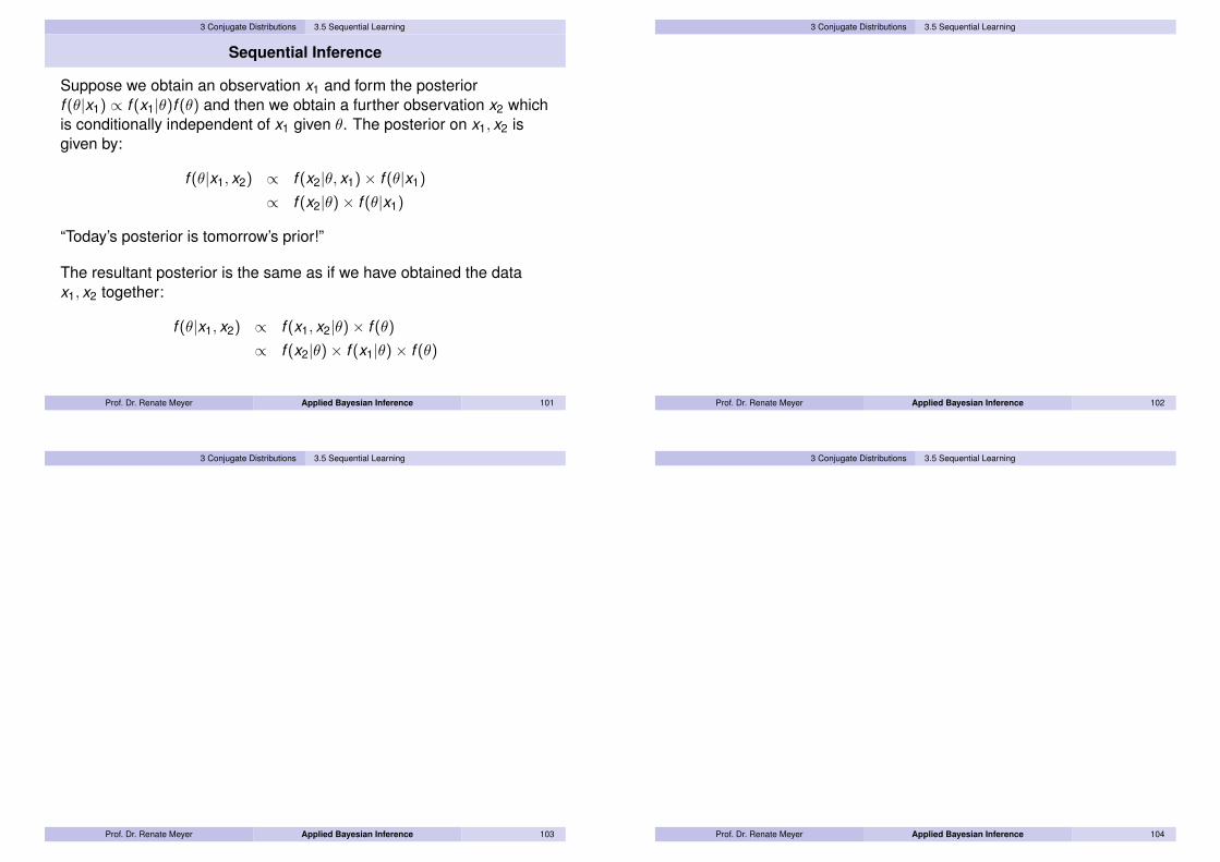
Sequential Inference
Suppose we obtain an observation x1 and form the posteriorf (θ|x1) ∝ f (x1|θ)f (θ) and then we obtain a further observation x2 whichis conditionally independent of x1 given θ. The posterior on x1, x2 isgiven by:
f (θ|x1, x2) ∝ f (x2|θ, x1)× f (θ|x1)
∝ f (x2|θ)× f (θ|x1)
“Today’s posterior is tomorrow’s prior!”
The resultant posterior is the same as if we have obtained the datax1, x2 together:
f (θ|x1, x2) ∝ f (x1, x2|θ)× f (θ)
∝ f (x2|θ)× f (x1|θ)× f (θ)
Prof. Dr. Renate Meyer Applied Bayesian Inference 101
3 Conjugate Distributions 3.5 Sequential Learning
Prof. Dr. Renate Meyer Applied Bayesian Inference 102
3 Conjugate Distributions 3.5 Sequential Learning
Prof. Dr. Renate Meyer Applied Bayesian Inference 103
3 Conjugate Distributions 3.5 Sequential Learning
Prof. Dr. Renate Meyer Applied Bayesian Inference 104

3 Conjugate Distributions 3.6 Comparing Bayesian and Frequentist Inference for Proportion
Comparing Bayesian and Frequentist Inference for Proportion
Frequentist inference is concerned withI point estimation,I interval estimation,I and hypothesis testing.
Prof. Dr. Renate Meyer Applied Bayesian Inference 105
3 Conjugate Distributions 3.6 Comparing Bayesian and Frequentist Inference for Proportion
Point Estimation
A single statistic is calculated from the sample data and used toestimate the unknown parameter.The statistic depends on the random sample, so it is random, and itsdistribution is called its sampling distribution.We call the statistic an estimator of the parameter and the value ittakes for the actual sample data an estimate.There are various frequentist approaches for finding estimators, suchas
I Least Squares (LS),I maximum likelihood estimation (MLE) andI uniformly minimum variance unbiased estimation (UMVUE).
For estimating the binomial parameter θ, the LS, MLE and UMVUE ofthe population proportion is the sample proportion.
Prof. Dr. Renate Meyer Applied Bayesian Inference 106
3 Conjugate Distributions 3.6 Comparing Bayesian and Frequentist Inference for Proportion
Bias
From a Bayesian perspective, point estimation means summarizing theposterior distribution by a single statistic, such as the posterior mean,median or mode. Here, we will use the posterior mean as the Bayesianpoint estimate (it minimizes the posterior mean squared error to give adecision-theoretic justification).
An estimator is said to be unbiased if the mean of its samplingdistribution is the true parameter, i.e. θ is unbiased if
E [θ] =
∫θf (θ|θ)d θ = θ,
where f (θ|θ) is the sampling distribution of the estimator θ given theparameter θ. The bias of an estimator θ is
bias(θ) = E [θ]− θ.
(Bayes estimators are usually biased.)Prof. Dr. Renate Meyer Applied Bayesian Inference 107
3 Conjugate Distributions 3.6 Comparing Bayesian and Frequentist Inference for Proportion
Mean Squared Error
An estimator is said to be a minimum variance unbiased estimator if noother unbiased estimator has a smaller variance. However, it ispossible that there may be a biased estimator that, on average, iscloser to the true value than the unbiased estimator. We need to lookat the possible trade-off between bias and variance.The (frequentist) mean squared error of an estimator θ is the averagesquared distance the estimator is away from the true value:
MS(θ) = E [(θ − θ)2] =
∫(θ − θ)2f (θ|θ)d θ.
One can show that
MS(θ) = bias(θ)2 + Var(θ).
Thus, it gives a better frequentist criterion for judging estimators thanthe bias or the variance alone.
Prof. Dr. Renate Meyer Applied Bayesian Inference 108

3 Conjugate Distributions 3.6 Comparing Bayesian and Frequentist Inference for Proportion
MSE Comparison
We will now compare the mean squared error of the Bayesian and thefrequentist estimator of the population proportion θ.The frequentist estimator for θ is
θf =Xn,
where X , the number of successes in n trials, has the Binomial(n, θ)distribution with mean and variance given by
E(X ) = nθ and Var(X ) = nθ(1− θ)
Thus,
E [θf ] = θ
Var(θf ) =θ(1− θ)
nMS(θf ) = 02 +
θ(1− θ)
nProf. Dr. Renate Meyer Applied Bayesian Inference 109
3 Conjugate Distributions 3.6 Comparing Bayesian and Frequentist Inference for Proportion
MSE Comparison
Suppose we use the posterior mean as the Bayesian estimate for θ,where we use the Beta(1,1) prior (uniform prior), thenθB = 1+x
n+2 = xn+2 + 1
n+2
Thus, the mean of its sampling distribution is
E [θB] = nθn+2 + 1
n+2
and the variance of its sampling distribution is
Var(θB) = 1(n+2)2 nθ(1− θ)
Hence, the mean squared error is
MS(θB) =
(nθ
n + 2+
1n + 2
− θ)2
+1
(n + 2)2 nθ(1− θ)
=
[1− 2θn + 2
]2
+1
(n + 2)2 nθ(1− θ)
Prof. Dr. Renate Meyer Applied Bayesian Inference 110
3 Conjugate Distributions 3.6 Comparing Bayesian and Frequentist Inference for Proportion
MSE ComparisonFor example, suppose θ = 0.4 and the sample size is n = 10. Then
MS(θf ) = 0.4×0.610 = 0.024
and
MS(θB) = 0.0169
Next, suppose θ = 0.5 and n = 10. Then
MS(θf ) = 0.025
and
MS(θB) = 0.01736
Prof. Dr. Renate Meyer Applied Bayesian Inference 111
3 Conjugate Distributions 3.6 Comparing Bayesian and Frequentist Inference for Proportion
MSE Comparison
Figure 8 shows the mean squared error for the Bayesian and thefrequentist estimator as a function of θ. Over most (but not all) of therange, the Bayesian estimator (using uniform prior) performs betterthat the frequentist estimator.
theta
MSE
0.0 0.2 0.4 0.6 0.8 1.0
0.00.0
050.0
100.0
150.0
200.0
25
Bayesfrequentist
Figure 8: Mean squared error for the two estimates.
Prof. Dr. Renate Meyer Applied Bayesian Inference 112

3 Conjugate Distributions 3.6 Comparing Bayesian and Frequentist Inference for Proportion
Interval Estimation
The aim is to find an interval (l ,u) that has a predetermined probabilityof containing the parameter
P(l ≤ θ ≤ u) = 1− α.
In the frequentist interpretation, the parameter is fixed but unknownand, before the sample is taken, the interval endpoints are randombecause they depend on the data. After the sample is taken, and theendpoints are calculated, there is nothing random, so the interval iscalled a confidence interval for the parameter. Under the frequentistparadigm, the correct interpretation for a (1− α)× 100% confidenceinterval is that (1− α)× 100% of the random intervals calculated thisway will contain the true value. Often, the sampling distribution of theestimator is approximately normal or tn−1 distributed with mean equalto the true value.
Prof. Dr. Renate Meyer Applied Bayesian Inference 113
3 Conjugate Distributions 3.6 Comparing Bayesian and Frequentist Inference for Proportion
Confidence – Credible Interval
In this case, the confidence interval has the form
estimator ± critical value × stdev of estimator ,
where the critical value comes from the normal or t table. For thesample proportion, an approximate (1− α)× 100% confidence intervalfor θ is given by:
θf ± tn−1(α/2)
√θf (1− θf )
n.
A Bayesian credible interval for the parameter θ on the other hand, hasthe natural interpretation that we want. Because it is found from theposterior distribution of θ, it has the coverage probability we want forthis specific data.
Prof. Dr. Renate Meyer Applied Bayesian Inference 114
3 Conjugate Distributions 3.6 Comparing Bayesian and Frequentist Inference for Proportion
Example: Interval Estimation
Example 3.1Out of a random sample of 100 Hamilton residents, x = 26 said theysupport a casino in Hamilton. Compare the frequentist 95% confidenceinterval with the Bayesian credible interval (using a uniform prior).
Frequentist 95% confidence interval:
0.26± 1.96×√
0.26× 0.74100
= (0.174,0.346)
Bayesian 95% credible interval:prior: Beta(1,1) posterior: Beta(1 + 26,1 + 74) =Beta(27,75)
> lu=qbeta(c(0.025,0.975),27,75)> lu[1] 0.1841349 0.3540134
Prof. Dr. Renate Meyer Applied Bayesian Inference 115
3 Conjugate Distributions 3.6 Comparing Bayesian and Frequentist Inference for Proportion
Hypothesis Testing
Example 3.2Suppose we wish to determine whether a new treatment is better thanthe standard treatment. If so, θ, the proportion of patients who benefitfrom the new treatment, should be higher than θ0, the proportion whobenefit from the standard treatment. It is known from historical recordsthat θ0 = .6. A random group of 10 patients are given the newtreatment. X , the number who benefit from the treatment will beBinomial(n, θ). We observe x = 8 patients benefit. This is better thanwe would expect if θ = 0.6. But, is it sufficiently better for us toconclude that θ > 0.6 at the 5% level of significance?The following table gives the null distribution of X :
x 0 1 2 3 4 5 6 7 8 9 10f (x|θ0) .001 .0016 .0106 .0425 .1115 .2007 .2508 .2150 .1209 .0403 .0060
Prof. Dr. Renate Meyer Applied Bayesian Inference 116

3 Conjugate Distributions 3.6 Comparing Bayesian and Frequentist Inference for Proportion
Frequentist Test
H0 : θ ≤ 0.6 H1 : θ > 0.6
Under H0: X |θ = 0.6 ∼ Binomial(10,0.6)
P-value
= P(X ≥ 8|H0 true)= P(X ≥ 8|θ = 0.6)= 1− pbinom(7,10,0.6)= 0.1209 + 0.0403 + 0.0060 = 0.1672 > 0.05 =⇒ not reject H0
Prof. Dr. Renate Meyer Applied Bayesian Inference 117
3 Conjugate Distributions 3.6 Comparing Bayesian and Frequentist Inference for Proportion
Bayesian Test
prior: Beta(1,1)data: x = 8, n − x = 2posterior: Beta(9,3)
P(H0|x = 8) = P(θ ≤ 0.6|x = 8)
= pbeta(0.6,9,3)
= 0.1189
Prof. Dr. Renate Meyer Applied Bayesian Inference 118
3 Conjugate Distributions 3.6 Comparing Bayesian and Frequentist Inference for Proportion
Prof. Dr. Renate Meyer Applied Bayesian Inference 119
3 Conjugate Distributions 3.6 Comparing Bayesian and Frequentist Inference for Proportion
Prof. Dr. Renate Meyer Applied Bayesian Inference 120
3 Conjugate Distributions 3.7 Exponential Distribution
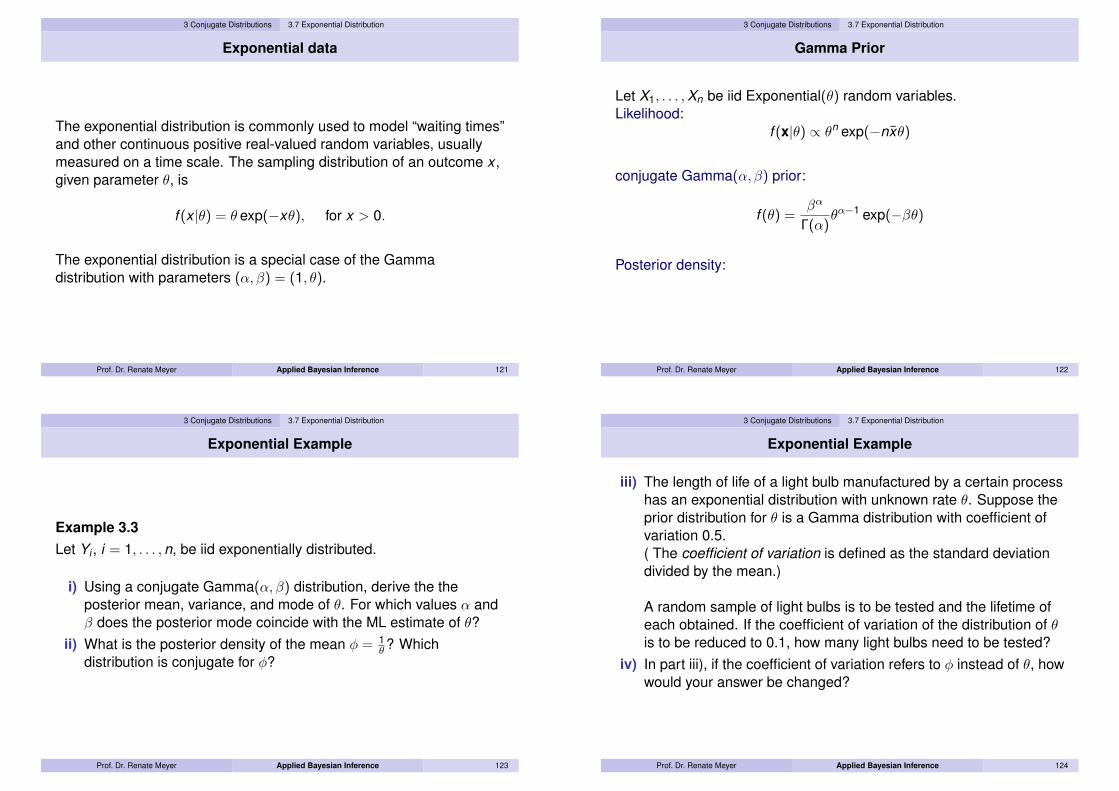
Exponential data
The exponential distribution is commonly used to model “waiting times”and other continuous positive real-valued random variables, usuallymeasured on a time scale. The sampling distribution of an outcome x ,given parameter θ, is
f (x |θ) = θ exp(−xθ), for x > 0.
The exponential distribution is a special case of the Gammadistribution with parameters (α, β) = (1, θ).
Prof. Dr. Renate Meyer Applied Bayesian Inference 121
3 Conjugate Distributions 3.7 Exponential Distribution
Gamma Prior
Let X1, . . . ,Xn be iid Exponential(θ) random variables.Likelihood:
f (x|θ) ∝ θn exp(−nxθ)
conjugate Gamma(α, β) prior:
f (θ) =βα
Γ(α)θα−1 exp(−βθ)
Posterior density:
f (θ|x) ∝ θn+α−1 exp(−θ(nx + β)) ∼ Gamma(α + n, β + nx)
Prof. Dr. Renate Meyer Applied Bayesian Inference 122
3 Conjugate Distributions 3.7 Exponential Distribution
Exponential Example
Example 3.3Let Yi , i = 1, . . . ,n, be iid exponentially distributed.
i) Using a conjugate Gamma(α, β) distribution, derive the theposterior mean, variance, and mode of θ. For which values α andβ does the posterior mode coincide with the ML estimate of θ?
ii) What is the posterior density of the mean φ = 1θ? Which
distribution is conjugate for φ?
Prof. Dr. Renate Meyer Applied Bayesian Inference 123
3 Conjugate Distributions 3.7 Exponential Distribution
Exponential Example
iii) The length of life of a light bulb manufactured by a certain processhas an exponential distribution with unknown rate θ. Suppose theprior distribution for θ is a Gamma distribution with coefficient ofvariation 0.5.( The coefficient of variation is defined as the standard deviationdivided by the mean.)
A random sample of light bulbs is to be tested and the lifetime ofeach obtained. If the coefficient of variation of the distribution of θis to be reduced to 0.1, how many light bulbs need to be tested?
iv) In part iii), if the coefficient of variation refers to φ instead of θ, howwould your answer be changed?
Prof. Dr. Renate Meyer Applied Bayesian Inference 124

3 Conjugate Distributions 3.7 Exponential Distribution
Prof. Dr. Renate Meyer Applied Bayesian Inference 125
3 Conjugate Distributions 3.7 Exponential Distribution
Prof. Dr. Renate Meyer Applied Bayesian Inference 126
3 Conjugate Distributions 3.7 Exponential Distribution
Prof. Dr. Renate Meyer Applied Bayesian Inference 127
3 Conjugate Distributions 3.7 Exponential Distribution
Prof. Dr. Renate Meyer Applied Bayesian Inference 128

3 Conjugate Distributions 3.8 Poisson Distribution
Poisson Data
Let X be the number of times a certain event occurs in a unit interval oftime and the following conditions hold
I The events are occurring at a constant average rate of θ per unittime.
I The number of events in any one interval of time is statisticallyindependent of the number in any other nonoverlapping interval.
I The probability of more than one event occurring in an interval oflength d goes to zero as d goes to zero.
Any process producing events which satisfy the above three axioms iscalled a Poisson process and X , the number of events in a unit timeinteral, is distributed as Poisson(θ).
Prof. Dr. Renate Meyer Applied Bayesian Inference 129
3 Conjugate Distributions 3.8 Poisson Distribution
Gamma Prior
Let X be a Poisson(θ) random variable and we observe X = x .Likelihood:
f (x |θ) =θx e−θ
x!
∝ θx e−θ
Conjugate Gamma(α, β) prior:
f (θ) =βα
Γ(α)θα−1 exp(−βθ)
∝ θα−1 exp(−βθ)
Prof. Dr. Renate Meyer Applied Bayesian Inference 130
3 Conjugate Distributions 3.8 Poisson Distribution
Calculating Posterior
Posterior density:
f (θ|x) ∝ f (θ)f (x |θ)
∝ θα−1e−βθθx e−θ
∝ θα+x−1e−θ(β+1)
i.e. pdf of Gamma(α + x , β + 1)
Prof. Dr. Renate Meyer Applied Bayesian Inference 131
3 Conjugate Distributions 3.8 Poisson Distribution
Prior Predictive Distribution
Prior predictive distribution for X : f (x)
f (x) =
∫ ∞0
f (x |θ)f (θ)dθ
=
∫ ∞0
θx e−θ
x!
βα
Γ(α)θα−1e−βθdθ
=βα
Γ(α)
1x!
∫ ∞0
θα+x−1e−(β+1)θdθ
=βα
Γ(α)
1x!
Γ(α + x)
(β + 1)α+x
=βα
(β + 1)α(β + 1)x(α + x − 1)!
(α− 1)!x!
=
(β
β + 1
)α( 1β + 1
)x (α + x − 1
x
)Prof. Dr. Renate Meyer Applied Bayesian Inference 132

3 Conjugate Distributions 3.8 Poisson Distribution
Negative Binomial
i.e. Negative-Binomial(α, β)
i.e. the no. of Bernoulli failures obtained before the α’th success whenthe success probability is p = β
β+1
which shows
Neg-bin(x |α, β) =
∫Poisson(x |θ)Gamma(θ|α, β)dθ
Prof. Dr. Renate Meyer Applied Bayesian Inference 133
3 Conjugate Distributions 3.8 Poisson Distribution
Multiple Poisson Data
Now let X1, . . . ,Xn be iid Poisson(θ) random variables. Suppose weobserve x = (x1, . . . , xn).
Likelihood:
f (x|θ) =n∏
i=1
f (xi |θ)
=n∏
i=1
θxi e−θ
xi !
=1∏n
i=1 xi !θ∑n
i=1 xi e−nθ
∝ θnx e−nθ
Prof. Dr. Renate Meyer Applied Bayesian Inference 134
3 Conjugate Distributions 3.8 Poisson Distribution
Multiple Poisson Data
Conjugate Gamma(α, β) prior:
f (θ) ∝ θα−1 exp(−βθ)
Posterior density:
f (θ|x) ∝ f (θ)f (x |θ)
∝ θα−1e−βθθnx e−nθ
∝ θα+nx−1e−θ(β+n)
i.e. pdf of Gamma(α + nx , β + n)
Prof. Dr. Renate Meyer Applied Bayesian Inference 135
3 Conjugate Distributions 3.8 Poisson Distribution
Poisson Example
Example 3.4Suppose that causes of death are reviewed in detail for a city in the USfor a single year. It is found that 3 persons, out of a population of200,000, died of asthma, giving a crude estimated asthma mortalityrate in the city of 1.5 per 100,000 persons per year. A Poissonsampling model is often used for epidemiological data of this form. Letθ represent the true underlying long-term asthma mortality rate in thecity (measured in cases per 100,000 persons per year). Reviews ofasthma mortality rates around the world suggest that mortality ratesabove 1.5 per 100,000 people are rare in Western countries, withtypical asthma mortality rates around 0.6 per 100,000.
a) Construct a conjugate prior density and derive the posteriordistribution of θ.
Prof. Dr. Renate Meyer Applied Bayesian Inference 136

3 Conjugate Distributions 3.8 Poisson Distribution
Poisson Example
b) What is the posterior probability that the long-term death rate fromasthma in the city is more than 1.0 per 100,000 per year?
c) What is the posterior predictive distribution of a future observationY ?
d) To consider the effect of additional data, suppose that ten years ofdata are obtained for the city in this example with y = 30 deathsover 10 years. Assuming the population is constant at 200,000,and assuming the outcomes in the ten years are independent withconstant long-term rate θ, derive the posterior distribution of θ.
e) What is the posterior probability that the long-term death rate fromasthma in the city is more than 1.0 per 100,000 per year?
Prof. Dr. Renate Meyer Applied Bayesian Inference 137
3 Conjugate Distributions 3.8 Poisson Distribution
Poisson Example
Prof. Dr. Renate Meyer Applied Bayesian Inference 138
3 Conjugate Distributions 3.8 Poisson Distribution
Poisson Example
Prof. Dr. Renate Meyer Applied Bayesian Inference 139
3 Conjugate Distributions 3.8 Poisson Distribution
Poisson Example
Prof. Dr. Renate Meyer Applied Bayesian Inference 140

3 Conjugate Distributions 3.9 Normal Distribution
Normal data, known variance, single data
A random variable X has a Normal distribution with mean µ andvariance σ2 if X has a continuous distribution with pdf
f (x) =1√2πσ
exp
[−1
2
(x − µσ
)2]
for −∞ < x <∞.
Prof. Dr. Renate Meyer Applied Bayesian Inference 141
3 Conjugate Distributions 3.9 Normal Distribution
Normal Example
Example 3.5According to Kennett and Ross (1983), Geochronology, London:Longmans, the first apparently reliable datings for the age of Ennerdalegranophyre were obtained from the K/Ar method (which depends onobserving the relative proportions of potassium-40 and argon-40 in therock) in the 1960s and early 1970s, and these resulted in an estimateof 370± 20 million years. Later in the 1970s, measurements based onthe Rb/Sr method (depending on the relative proportions ofrubidium-87 and strontium-87) gave an age of 421± 8 million years. Itappears that the errors marked are meant to be standard deviations,and it seems plausible that the errors are normally distributed. If then ascientist had the K/Ar measurements available in the early 1970s, thiscould be the basis of her prior beliefs about the age of these rocks.
Prof. Dr. Renate Meyer Applied Bayesian Inference 142
3 Conjugate Distributions 3.9 Normal Distribution
Normal Prior
Likelihood: X |µ ∼ N(µ, σ2), σ2 known
f (x |µ) =1√2πσ
exp(− 1
2σ2 (x − µ)2)∝ exp
(− 1
2σ2 (x − µ)2)
Conjugate prior: µ ∼ N(µ0, σ20), µ0, σ
20 are hyperparameters
f (µ) =1√
2πσ0exp
(− 1
2σ20
(µ− µ0)2
)∝ exp
(− 1
2σ20
(µ− µ0)2
)
Prof. Dr. Renate Meyer Applied Bayesian Inference 143
3 Conjugate Distributions 3.9 Normal Distribution
Calculating Posterior
Posterior: µ|x ∼ N(µ1, σ21)
where
µ1 =
1σ2
0µ0 + 1
σ2 x1σ2
0+ 1
σ2
1σ2
1=
1σ2
0+
1σ2
NB: posterior precision = prior precision + data precisionposterior mean = weighted average of prior mean and observation
Prof. Dr. Renate Meyer Applied Bayesian Inference 144

3 Conjugate Distributions 3.9 Normal Distribution
Calculating Posterior
f (µ|x)∝ f (x |µ)f (µ)
∝ exp
(−1
2
[(x − µ)2
σ2 +(µ− µ0)2
σ20
])
∝ exp
(− 1
2σ2 (x2 − 2xµ+ µ2)− 12σ2
0(µ2 − 2µµ0 + µ2
0)
)
∝ exp
(−1
2
[µ2
(1σ2 +
1σ2
0
)− 2µ
(xσ2 +
µ0
σ20
)+ const .
])
∝ exp
−12
1(1σ2 + 1
σ20
)−1
µ2 − 2µ
xσ2 + µ0
σ20
1σ2 + 1
σ20
+ const .
∝ exp
−12
1(1σ2 + 1
σ20
)−1
µ− xσ2 + µ0
σ20
1σ2 + 1
σ20
2
Prof. Dr. Renate Meyer Applied Bayesian Inference 145
3 Conjugate Distributions 3.9 Normal Distribution
Posterior Mean Expressions
Alternative expressions for posterior mean:
µ1 = µ0 + (x − µ0)σ2
0
σ2 + σ20
prior mean adjusted towards observed value
µ1 = x − (x − µ0)σ2
σ2 + σ20
data shrunk towards prior mean
Prof. Dr. Renate Meyer Applied Bayesian Inference 146
3 Conjugate Distributions 3.9 Normal Distribution
Prior Predictive Distribution
Prior predictive distribution of X : X ∼ N(µ0, σ2 + σ2
0)
Because:
f (x) =∫
f (x |µ)f (µ)dµ
f (x , µ) = f (x |µ)f (µ) ∝ exp(− 1
2σ2 (x − µ)2 − 12σ2
0(µ− µ0)2
)i.e. (X , µ) have a bivariate normal distributionthen the marginal distribution of X is normal
Now:
E [X ] = E [E [X |µ]] = E [µ] = µ0
Var(X ) = E [Var(X |µ)] + Var(E [X |µ])
= E [σ2] + Var(µ) = σ2 + σ20
Prof. Dr. Renate Meyer Applied Bayesian Inference 147
3 Conjugate Distributions 3.9 Normal Distribution
Reminder: Conditional Mean and Variance
If U and V are random variables, then
E [U] = E [E [U|V ]]
Var(U) = E [Var(U|V )] + Var(E [U|V ])
Prof. Dr. Renate Meyer Applied Bayesian Inference 148

3 Conjugate Distributions 3.9 Normal Distribution
Posterior Predictive Distribution
Posterior predictive distribution of future Y :Y |x ∼ N(µ1, σ
2 + σ21) Because:
f (y |x) =∫
f (y |µ)f (µ|x)dµ
f (y , µ|x) = f (y |µ)f (µ|x) ∝ exp(− 1
2σ2 (y − µ)2 − 12σ2
1(µ− µ1)2
)i.e. (Y , µ)|x have a bivariate normal distributionthen the marginal distribution of Y |x is normalNow:E [Y |x ] = E [E [Y |µ]|x ] = E [µ|x ] = µ1
Var(Y |x) = E [Var(Y |µ)|x ] + Var(E [Y |µ]|x)
= E [σ2|x ] + Var(µ|x) = σ2 + σ21
Prof. Dr. Renate Meyer Applied Bayesian Inference 149
3 Conjugate Distributions 3.9 Normal Distribution
Normal Example
Now back to Example 3.5:
Single Normal observation, Normal prior
mu
dens
ity
300 350 400 450
0.00.0
10.0
20.0
30.0
40.0
5
priorposteriorlikelihood
Figure 9: Conjugate Normal prior and single observation.
Prof. Dr. Renate Meyer Applied Bayesian Inference 150
3 Conjugate Distributions 3.9 Normal Distribution
Normal data, known variance, multiple data
Example 3.6What is now called the National Institute of Standards and Technology(NIST) in Washington DC conducts extremely high precisionmeasurement of physical constants, such as the actual weight ofso-called check-weights that are supposed to serve as referencestandards (like the official kg). In 1962-63, for example, n = 100weighings of a block of metal called NB10, which was supposed toweigh exactly 10g, were made under conditions as close to iid aspossible. The 100 measurements x1, . . . , xn (the units are microgramsbelow 10g) have a mean of x = 404.6 and a SD of s = 6.5.
Prof. Dr. Renate Meyer Applied Bayesian Inference 151
3 Conjugate Distributions 3.9 Normal Distribution
Normal Example
weight frequency weight frequency375 1 406 12392 1 407 8393 1 408 5397 1 409 5398 2 410 4399 7 411 1400 4 412 3401 12 413 1402 8 415 1403 6 418 1404 9 423 1405 5 437 1
Prof. Dr. Renate Meyer Applied Bayesian Inference 152

3 Conjugate Distributions 3.9 Normal Distribution
Normal Example
Questions:
1. How much does NB10 really weigh?2. How certain are you given the data that the true weight of NB10 is
less than 405.25 µ g below 10g?3. What is the underlying accuracy of the NB10 measuring process?4. How accurately can you predict the 101st measurement?
A Normal qqplot shows that a Normal sampling distribution isappropriate. We first assume that σ2 is known.
Prof. Dr. Renate Meyer Applied Bayesian Inference 153
3 Conjugate Distributions 3.9 Normal Distribution
Calculting Posterior
Likelihood: Xi |µiid∼ N(µ, σ2), i = 1, . . . ,n, σ2 known
Conjugate prior: µ ∼ N(µ0, σ20), µ0, σ
20
Posterior: µ|x ∼ N(µn, σ2n)
where
µn =
1σ2
0µ0 + n
σ2 x1σ2
0+ n
σ2
1σ2
n=
1σ2
0+
nσ2
Prof. Dr. Renate Meyer Applied Bayesian Inference 154
3 Conjugate Distributions 3.9 Normal Distribution
Calculating Posterior
Why?
Reduction to the case of single data point of previous section:
If X1, . . . ,Xn|µiid∼ N(µ, σ2)
Likelihood: f (x1, . . . , xn|θ)
=∏n
i=1 f (xi |µ)=∏n
i=11√2πσ
exp[−1
2
(xi−µσ
)2]
= const. × exp[−1
2∑n
i=1( xi−µ
σ
)2]∝ . . . ∝exp
[−1
2
(x−µσ/√
n
)2]
Prof. Dr. Renate Meyer Applied Bayesian Inference 155
3 Conjugate Distributions 3.9 Normal Distribution
Calculating Posterior
∝ f (x |µ)
The likelihood depends on data x1, . . . , xn only through the sufficientstatistic x
and X |µ ∼ N(µ, σ2/n).
Thus, in previous section 3.9, simply substitute σ2 by σ2/n and x by x .
Prof. Dr. Renate Meyer Applied Bayesian Inference 156

3 Conjugate Distributions 3.9 Normal Distribution
Remarks
1. If σ20 = σ2 then
µn =µ0 + nxn + 1
=µ0 +
∑xi
n + 11σ2
n=
n + 1σ2
i.e. prior has weight of one additional observation with value µ0.
2. If n large, the posterior is determined by x and σ2.
3. If σ20 −→∞ (diffuse prior) and n fixed, then
µ|x ∼ N(x , σ2/n)
posterior mean = MLE
Prof. Dr. Renate Meyer Applied Bayesian Inference 157
3 Conjugate Distributions 3.9 Normal Distribution
Remarks
4. The prior info is equivalent to σ2
σ20
additional observations all equalto µ0 since
µn =
1σ2
0µ0 + n
σ2 x1σ2
0+ n
σ2
=
σ2
σ20µ0 +
∑xi
σ2
σ20
+ n
Prof. Dr. Renate Meyer Applied Bayesian Inference 158
3 Conjugate Distributions 3.9 Normal Distribution
Back to Normal Example
Prof. Dr. Renate Meyer Applied Bayesian Inference 159
3 Conjugate Distributions 3.9 Normal Distribution
Back to Normal Example
Prof. Dr. Renate Meyer Applied Bayesian Inference 160

3 Conjugate Distributions 3.9 Normal Distribution
Back to Normal Example
Multiple Normal observations, Normal prior
mu
dens
ity
360 380 400 420 440
0.00.1
0.20.3
0.40.5
0.6
priorposteriorlikelihood
Figure 10: Conjugate Normal prior and several observations.
Prof. Dr. Renate Meyer Applied Bayesian Inference 161
3 Conjugate Distributions 3.9 Normal Distribution
Normal data, known variance, noninformative prior
Example 3.7Changes in blood pressure (in mmHg) were recorded for each of 100
patients, where negative numbers are decreases while on the drugand positive numbers are increases:
+3.7− 6.7− 10.5 . . .− 16.7− 7.2
with sample mean x = −7.99 and standard deviation s = 4.33.
We will assume that the change in blood pressure X has a Normaldistribution with unknown mean µ and known variance σ2 = 4.332.
Prof. Dr. Renate Meyer Applied Bayesian Inference 162
3 Conjugate Distributions 3.9 Normal Distribution
Example
Let us assume that we don’t know anything about the mean change inblood pressure induced by the new drug and thus assume that θ canattain any real value with equal probability. This gives a flat priordistribution for µ on (−∞,∞), i.e.
f (µ) ∝ 1.
(There is no “proper” continuous uniform distribution on (−∞,∞), butyou can think of µ being uniform on some finite interval (−a,a), forsome large a and ignore the normalization constant, as it is notneeded for the application of Bayes’ theorem).
What is the posterior distribution of µ?
Prof. Dr. Renate Meyer Applied Bayesian Inference 163
3 Conjugate Distributions 3.9 Normal Distribution
Calculating Posterior
Posterior pdf: f (µ|x)
∝ prior × likelihood
∝ f (µ)f (x |µ)
∝ 1× exp[−1
2
(x−µσ/√
n
)2]
∝ exp[−1
2
(µ−xσ/√
n
)2]
∝ pdf of Normal(x , σ2/n)
Prof. Dr. Renate Meyer Applied Bayesian Inference 164

3 Conjugate Distributions 3.9 Normal Distribution
Simple Updating Rule
If Xiiid∼ Normal(µ, σ2), i = 1, . . . ,n and a flat prior is used, then the
posterior distribution of µ|x is
Normal(θn, σ2n) with
θn = x and
σ2n = σ2/n.
In Example 3.7
θn = −7.99
σ2n = 4.332/100 = 0.187489
Prof. Dr. Renate Meyer Applied Bayesian Inference 165
3 Conjugate Distributions 3.9 Normal Distribution
Credible Intervals
95% posterior probability interval for µ:
µL = 2.5% quantile of N(−7.99,0.187489)
µU = 97.5% quantile of N(−7.99,0.187489)
In R:
> lu=qnorm(c(0.025,0.975),-7.99,sqrt(0.187489))> lu[1] -8.838664 -7.141336
Prof. Dr. Renate Meyer Applied Bayesian Inference 166
3 Conjugate Distributions 3.9 Normal Distribution
Hypothesis Test
Test the null hypothesis H0 : µ ≤ −7.0.
P(H0|x) = P(µ ≤ −7.0|x)
In R:
> p=pnorm(-7,-7.99,sqrt(0.187489))> p[1] 0.9888838
Prof. Dr. Renate Meyer Applied Bayesian Inference 167
3 Conjugate Distributions 3.9 Normal Distribution
Prof. Dr. Renate Meyer Applied Bayesian Inference 168

3 Conjugate Distributions 3.9 Normal Distribution
2-Parameter Normal with Conjugate Prior
prior distribution:
µ|σ2 ∼ N(µ0, σ2/κ0)
σ2 ∼ Inv-χ2(ν0, σ20)
where Inv-χ2(ν0, σ20) denotes the scaled inverse χ2-distribution with
scale σ20 and ν0 degrees of freedom, i.e. the distribution of σ2
0ν0/Zwhere Z is a χ2 random variable with ν0 degrees of freedom.joint prior density:
f (µ, σ2) ∝ σ−1(σ2)−(ν0/2+1) exp(− 1
2σ2 [ν0σ20 + κ0(µ0 − µ)2]
)∼ N-Inv-χ2(µ0, σ
20/κ0, ν0, σ
20)
Prof. Dr. Renate Meyer Applied Bayesian Inference 169
3 Conjugate Distributions 3.9 Normal Distribution
2-Parameter Normal with Conjugate Prior
joint posterior density:
f (µ, σ2|x) ∝ σ−1(σ2)−(ν0/2+1) exp(− 1
2σ2 [ν0σ20 + κ0(µ0 − µ)2]
)×(σ2)−n/2 exp
(− 1
2σ2 [(n − 1)s2 + n(x − µ)2]
)∼ N-Inv-χ2(µn, σ
2n/κn, νn, σ
2n)
where
µn =κ0
κ0 + nµ0 +
nκ0 + n
x
κn = κ0 + nνn = ν0 + n
νnσ2n = ν0σ
20 + (n − 1)s2 +
κ0nκ0 + n
(x − µ0)2.
Prof. Dr. Renate Meyer Applied Bayesian Inference 170
3 Conjugate Distributions 3.9 Normal Distribution
2-Parameter Normal with Conjugate Prior
conditional posterior of µ:
µ|σ2,x ∼ N(µn, σ2/κn)
= N
(κ0σ2µ0 + n
σ2 xκ0σ2 + n
σ2
,1
κ0σ2 + n
σ2
)
marginal posterior of σ2:
σ2|x ∼ Inv-χ2(νn, σ2n)
marginal posterior of µ:
f (µ|x) ∝[1 +
κn(µ− µn)2
νnσ2n
]−(νn+1)/2
∼ tνn (µ|µn, σ2n/κn)
Prof. Dr. Renate Meyer Applied Bayesian Inference 171
3 Conjugate Distributions 3.9 Normal Distribution
Prof. Dr. Renate Meyer Applied Bayesian Inference 172
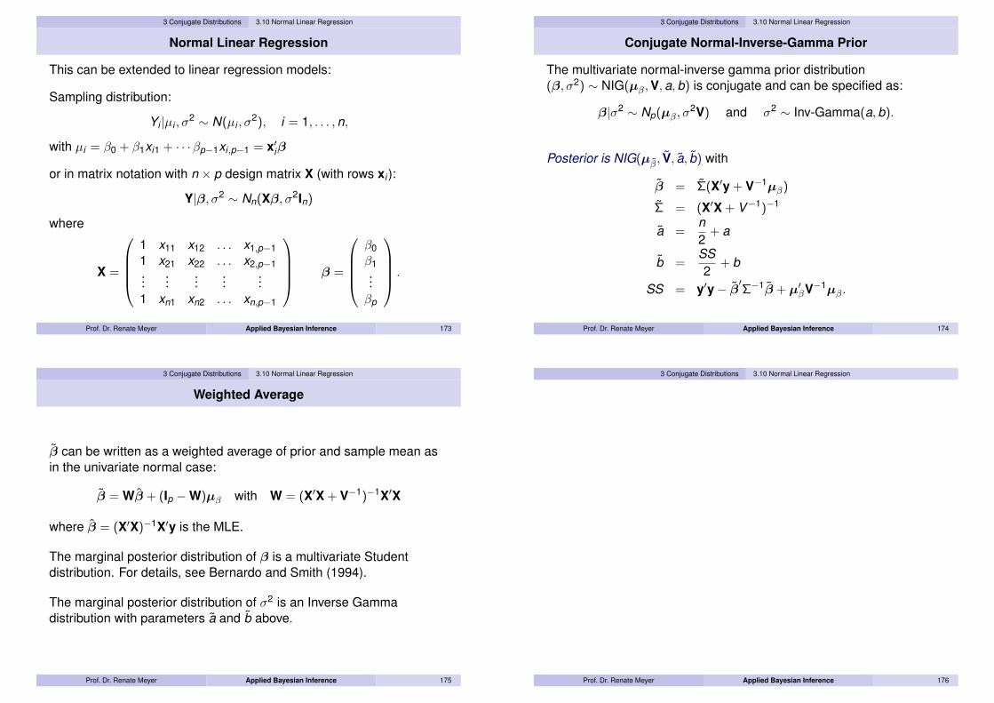
3 Conjugate Distributions 3.10 Normal Linear Regression
Normal Linear Regression
This can be extended to linear regression models:
Sampling distribution:
Yi |µi , σ2 ∼ N(µi , σ
2), i = 1, . . . ,n,
with µi = β0 + β1xi1 + · · ·βp−1xi,p−1 = x′iβ
or in matrix notation with n × p design matrix X (with rows xi ):
Y|β, σ2 ∼ Nn(Xβ, σ2In)
where
X =
1 x11 x12 . . . x1,p−11 x21 x22 . . . x2,p−1...
......
......
1 xn1 xn2 . . . xn,p−1
β =
β0β1...βp
.
Prof. Dr. Renate Meyer Applied Bayesian Inference 173
3 Conjugate Distributions 3.10 Normal Linear Regression
Conjugate Normal-Inverse-Gamma Prior
The multivariate normal-inverse gamma prior distribution(β, σ2) ∼ NIG(µβ,V,a,b) is conjugate and can be specified as:
β|σ2 ∼ Np(µβ, σ2V) and σ2 ∼ Inv-Gamma(a,b).
Posterior is NIG(µβ, V, a, b) with
β = Σ(X′y + V−1µβ)
Σ = (X′X + V−1)−1
a =n2
+ a
b =SS2
+ b
SS = y′y− β′Σ−1β + µ′βV−1µβ.
Prof. Dr. Renate Meyer Applied Bayesian Inference 174
3 Conjugate Distributions 3.10 Normal Linear Regression
Weighted Average
β can be written as a weighted average of prior and sample mean asin the univariate normal case:
β = Wβ + (Ip −W)µβ with W = (X′X + V−1)−1X′X
where β = (X′X)−1X′y is the MLE.
The marginal posterior distribution of β is a multivariate Studentdistribution. For details, see Bernardo and Smith (1994).
The marginal posterior distribution of σ2 is an Inverse Gammadistribution with parameters a and b above.
Prof. Dr. Renate Meyer Applied Bayesian Inference 175
3 Conjugate Distributions 3.10 Normal Linear Regression
Prof. Dr. Renate Meyer Applied Bayesian Inference 176

4 WinBUGS Applications 4.1 WinBUGS Handouts
WinBUGS Applications: Overview
Calculation of the posterior distribution is difficult in situations with:I nonconjugate priorsI multiple parameters
as we need to calculate summary statistics, like mean and variance,and in high-dim. problems, calculate marginal posterior distributions.All this involves integration, which has been a very big hurdle forBayesian inference in the past.
For low parameter dimensions, say 2,3,4,5 numerical integrationtechniques, asymptotic approximations etc may be used but thesebreak down for higher dimensions.
Prof. Dr. Renate Meyer Applied Bayesian Inference 177
4 WinBUGS Applications 4.1 WinBUGS Handouts
WinBUGS Applications: Overview
The most successful approach, for reasons that we will discuss in thesubsequent sections, is based on simulation. That means, instead ofexplicitly calculating the posterior and performing integrations, wegenerate a sample from the posterior distribution and use that sampleto approximate any quantity of interest, e.g. approximate the posteriormean by the sample mean etc.A very versatile software to do these posterior simulations isWinBUGS, the Windows version of BUGS (Bayesian inference UsingGibbs Sampling), developed by David Spiegelhalter and colleagues atthe MRC Biostatistics Unit of Cambridge University, England.
Prof. Dr. Renate Meyer Applied Bayesian Inference 178
4 WinBUGS Applications 4.1 WinBUGS Handouts
WinBUGS Applications: Overview
WinBUGS uses the Gibbs sampler to generate samples from theposterior distribution of parameters of a Bayesian model. We willdiscuss the Gibbs sampler and other Markov chain Monte Carlotechniques in detail in Chapter 6. For now, we simply consider thesimulation method used in WinBUGS as a black box but simply keep inmind, that the samples generated are not independent but dependent,i.e. they are samples from a Markov chain that converges towards theposterior distribution. Therefore, we can use the samples only from apoint in time where convergence has set in and need to discard theinitial so-called burn-in samples.
Prof. Dr. Renate Meyer Applied Bayesian Inference 179
4 WinBUGS Applications 4.1 WinBUGS Handouts
WinBUGS Handouts
We illustrate this sampling-based approach using our familiar exampleof Binomial data with a conjugate prior distribution and refer to thehandout
Brief Introduction to WinBUGS
Other handouts will discuss running WinBUGS in batch mode, fromwithin R using R2WinBUGS and how to use the R package CODA forconvergence diagnostics.Once familiar with WinBUGS, we will look at the huge range ofBayesian models, especially Bayesian hierarchical models, that can behandled with WinBUGS and concentrate on practical implementationissues rather than theory. The underlying theory will be recouped inthe subsequent chapters.
Prof. Dr. Renate Meyer Applied Bayesian Inference 180

4 WinBUGS Applications 4.2 Bayesian Linear Regression
Simple Linear Regression
In regression analysis, we look at the conditional distribution of theresponse variable at different levels of a predictor variable
I Response variable YI also called dependent or outcome variableI what we want to explain or predictI in simple linear regression, the response variable is continuous
I Predictor variables X1, . . . ,XpI also called independent variables or covariatesI in simple linear regression, the predictor variable is usually
continuousI which variable is response and which is predictor depends on our
research question
Prof. Dr. Renate Meyer Applied Bayesian Inference 181
4 WinBUGS Applications 4.2 Bayesian Linear Regression
Example
Example 4.1This example investigates the quality of the delivery system network ofa softdrink company, see Example 5.1 in Ntzoufras (2009). One isinterested in estimating the time each employee needs to refill anautomatic vending machine owned and served by the company. Forthis reason, a small quality assurance study was set up by an industrialengineer of the company. The response variable is the total servicetime (measured in minutes) of each machine, including its stockingwith beverages and any required maintenance or housekeeping. Afterexamining the problem, the industrial engineer recommends twoimportant variables that affect delivery time: the number of cases ofstocked products and the distance walked by the employee (measuredin feet). A dataset of 25 observations was finally collected.
Prof. Dr. Renate Meyer Applied Bayesian Inference 182
4 WinBUGS Applications 4.2 Bayesian Linear Regression
Data: Softdrink Delivery Times
Delivery Time Cases Distance16.68 7 56011.5 3 22012.03 3 34014.88 4 8013.75 6 15018.11 7 3308 2 11017.83 7 21079.24 30 146021.5 5 60540.33 16 68821 10 21513.5 4 25519.75 6 46224 9 44829 10 77615.35 6 20019 7 1329.5 3 3635.1 17 77017.9 10 14052.32 26 81018.75 9 45019.83 8 63510.75 4 150
Prof. Dr. Renate Meyer Applied Bayesian Inference 183
4 WinBUGS Applications 4.2 Bayesian Linear Regression
Model Assumptions
The explanatory variables are assumed fixed, their values denoted byxi1, . . . , xip for i = 1, . . . ,n. Given the values of the explanatoryvariables, the observations of the response variable are assumedindependent, normally distributed
Yi |xi1, . . . , xip ∼ N(µi , σ2) with
µi = β0 + β1xi1 + · · ·+ βpxip for i = 1, . . . ,n
or in matrix notation:
Y|x ∼ Nn(µ, σ2I) withµ = Xβ
where σ2 and β = (β0, β1, . . . , βp) is the set of regression parameters, Idenotes the identity matrix, Y the vector of observations and X = (xij)the n × (p + 1) design matrix.
Prof. Dr. Renate Meyer Applied Bayesian Inference 184

4 WinBUGS Applications 4.2 Bayesian Linear Regression
Likelihood Specification in WinBUGS
Note that in WinBUGS the normal distribution is parametrized in termsof the precision τ = 1
σ2 . The likelihood is thus specified by:
for (i in 1:n){y[i] ~ dnorm(mu[i],tau)mu[i] <- beta0 + beta1*x1[i] + ... + betap*xp[i]
}sigma2 <- 1/tausigma <- sqrt(sigma2)
Prof. Dr. Renate Meyer Applied Bayesian Inference 185
4 WinBUGS Applications 4.2 Bayesian Linear Regression
Prior Specification
In normal regression models, the simplest approach is to assume thatall parameters are a priori independent, i.e.
f (β, τ) =
p∏j=0
f (βj)f (τ)
βj ∼ N(µj , c2j ) for j = 0, . . . ,p
τ ∼ Gamma(a,b)
Thus, the precision has a prior mean of E(τ) = ab and prior variance
Var(τ) = ab2 . This corresponds to an Inverse Gamma prior distribution
for σ2 with E(σ2) = ba−1 and Var(σ2) = b2
(a−1)2(a−2).
No info about βj : µj = 0 and c2j = 10000.
No info about τ : a = b = 0.001
Prof. Dr. Renate Meyer Applied Bayesian Inference 186
4 WinBUGS Applications 4.2 Bayesian Linear Regression
Prior Specification in WinBUGS
beta0 ~ dnorm(0.0,1.0E-4)beta1 ~ dnorm(0.0,1.0E-4)....betap ~ dnorm(0.0,1.0E-4)tau ~ dgamma(0.001,0.001)
Prof. Dr. Renate Meyer Applied Bayesian Inference 187
4 WinBUGS Applications 4.2 Bayesian Linear Regression
Interpretation of Regression Coefficients
Each regression coefficient βj measures the effect of the explanatoryvariable Xj on the expected value of the response variable Y adjustedfor the remaining covariates.Questions of interest are
1. Is the effect of Xj important for the description of Y ?2. What is the association between Y and Xj (positive or negative)?3. What is the magnitude of the effect of Xj on Y?
Prof. Dr. Renate Meyer Applied Bayesian Inference 188

4 WinBUGS Applications 4.2 Bayesian Linear Regression
Interpretation of Regression Coefficients
Answers:1. Look at posterior distribution of βj and its credible interval. Does
the credible interval contain 0?
2. Calculate the posterior probability P(βj > 0) and P(βj < 0).In WinBUGS, use the step function
p.betaj <- step(betaj)
which creates a binary node p.betaj taking values 1 if βj > 0and 0 otherwise.
3. Posterior mean/median of βj is a measure of the posteriorexpected change of the response variable Y if Xj increases by 1unit and all other covariates are fixed.
Prof. Dr. Renate Meyer Applied Bayesian Inference 189
4 WinBUGS Applications 4.2 Bayesian Linear Regression
Interpretation of β0
β0 measures the posterior expected value of Y if all covariates arezero. Often, zero is not in the range of the covariates, and thus theinterpretation of β0 is not meaningful.Example: response: heart rate, covariate: body temperature indegrees CBetter: Center the covariates at their mean xc
ij = xij − xj
µi = βc0 + βc
1(xi1 − x1) + · · ·+ βc1(xip − xp)
βc0 = expected value of Y when all covariates are equal to their means
Centering the covariates is also advisable from a computational pointof view: it decreases the posterior correlation between parameters andthus improves convergence of the Gibbs sampler. We will show this inSection 6.
Prof. Dr. Renate Meyer Applied Bayesian Inference 190
4 WinBUGS Applications 4.2 Bayesian Linear Regression
Regression Example in WinBUGS
Prepare the data file by including variable names to be used byWinBUGS at the top of each column and END at the end and save asplain text file softdrinkdata.txt in your working directory.
time[] cases[] distance[]16.68 7 56011.5 3 22012.03 3 34014.88 4 8013.75 6 150...
......
35.1 17 77017.9 10 14052.32 26 81018.75 9 45019.83 8 63510.75 4 150END
For some odd reason (bug in WinBUGS?), make sure there is a blankline after END.
Prof. Dr. Renate Meyer Applied Bayesian Inference 191
4 WinBUGS Applications 4.2 Bayesian Linear Regression
Regression Example in R
Alternatively, if we want to fit a linear model in the frequentist way in Rfirst, to compare later on with the Bayesian results in WinBUGS, weread in the data, fit a linear model and output a list using dput(),using the following R commands:
softdrink <- read.table(file="softdrinkdata.txt",header=TRUE, sep="")attach(softdrink)cases_cent<- cases - mean(cases)distance_cent <- distance - mean(distance)summary(lm(time ~ cases_cent + distance_cent))dput(list(time=time,cases=cases,distance=distance)
"softdrinkdatalist.txt")
Prof. Dr. Renate Meyer Applied Bayesian Inference 192

4 WinBUGS Applications 4.2 Bayesian Linear Regression
Regression Output in R
Call:lm(formula = time ~ cases_cent + distance_cent)Residuals:
Min 1Q Median 3Q Max-5.7880 -0.6629 0.4364 1.1566 7.4197
Coefficients:Estimate Std. Error t value Pr(>|t|)
(Intercept) 22.384000 0.651895 34.337 < 2e-16 ***cases_cent 1.615907 0.170735 9.464 3.25e-09 ***distance_cent 0.014385 0.003613 3.981 0.000631 ***---Signif. codes: 0 ’***’ 0.001 ’**’ 0.01 ’*’ 0.05 ’.’ 0.1 ’ ’ 1
Residual standard error: 3.259 on 22 degrees of freedomMultiple R-squared: 0.9596, Adjusted R-squared: 0.9559F-statistic: 261.2 on 2 and 22 DF, p-value: 4.687e-16
Prof. Dr. Renate Meyer Applied Bayesian Inference 193
4 WinBUGS Applications 4.2 Bayesian Linear Regression
Regression Model in WinBUGS
model{# likelihoodfor (i in 1:n){
time[i] ~ dnorm( mu[i],tau)mu[i] <- beta0 + beta1*(cases[i]-mean(cases[])) +
beta2* (distance[i]-mean(distance[]))}
# prior distributionstau ~ dgamma(0.001,0.001)beta0 ~ dnorm(0.0,1.0E-4)beta1 ~ dnorm(0.0,1.0E-4)beta2 ~ dnorm(0.0,1.0E-4)
Prof. Dr. Renate Meyer Applied Bayesian Inference 194
4 WinBUGS Applications 4.2 Bayesian Linear Regression
Regression Model in WinBUGS
# definition of sigma, sigma2, and sd(Y)sigma2 <- 1/tausigma <- sqrt(sigma2)#calculation of Bayesian version of RsquaredR2B <- 1-sigma2/pow(sd(time[]),2)#posterior probabilitiesp.beta0 <- step(beta0)p.beta1 <- step(beta1)p.beta2 <- step(beta2)}#initslist(tau=1,beta0=1, beta1=0, beta2=0)
Prof. Dr. Renate Meyer Applied Bayesian Inference 195
4 WinBUGS Applications 4.2 Bayesian Linear Regression
Regression Output in WinBUGS
node mean sd MC error 2.5% median 97.5% start sampleR2B 0.9516 0.01732 7.742E-4 0.9063 0.9551 0.9737 1001 1000beta0 22.37 0.6681 0.02255 21.15 22.35 23.78 1001 1000beta1 1.61 0.1851 0.005237 1.254 1.606 1.992 1001 1000beta2 0.01447 0.003931 1.263E-4 0.006683 0.0144 0.02251 1001 1000p.beta0 1.0 0.0 3.162E-12 1.0 1.0 1.0 1001 1000p.beta1 1.0 0.0 3.162E-12 1.0 1.0 1.0 1001 1000p.beta2 1.0 0.0 3.162E-12 1.0 1.0 1.0 1001 1000sigma2 11.67 4.175 0.1866 6.364 10.82 22.7 1001 1000
Prof. Dr. Renate Meyer Applied Bayesian Inference 196

4 WinBUGS Applications 4.2 Bayesian Linear Regression
Bayesian Coefficient of Variation
A high value of the precision τ (low σ2) indicates that the model canaccurately predict the expected value of Y . We can rescale thisquantity using the sample variance of the response variable Y , s2
Y ,using the R2
B statistic given by:
R2B = 1− τ1
s2Y
= 1− σ2
s2Y.
This quantity can be interpreted as the proportional reduction ofuncertainty concerning the response variable Y achieved byincorporating the explanatory variables Xj in the model.
Prof. Dr. Renate Meyer Applied Bayesian Inference 197
4 WinBUGS Applications 4.2 Bayesian Linear Regression
Bayesian Coefficient of Variation
It can be regarded as the Bayesian analog of the adjusted coefficientof determination
R2adj = 1− σ2
s2Y,
where
σ2 =1
n − p
n∑i=1
(yi − yi)2 with yi = β0 +
p∑i=1
xij βj ,
where βj are the maximum likelihood estimates of βj .
Prof. Dr. Renate Meyer Applied Bayesian Inference 198
4 WinBUGS Applications 4.2 Bayesian Linear Regression
Missing Data
Missing data are easily incorporated in a Bayesian analysis.They are treated as unknown parameters to be estimated.Assume for instance, that observation 21 in the linear regressionExample 4.1 was missing, i.e. time[21] for cases[21]=10 anddistance[21]=140 was missing.In WinBUGS, missing values are denoted by NA in the dataset.Substituting 17.9 in the dataset by NA and running the code again, nowmonitoring the node time[21], we get the output
node mean sd MC error 2.5% median 97.5% start sampletime[21] 21.06 3.696 0.0821 13.71 21.02 28.4 1001 2000
Prof. Dr. Renate Meyer Applied Bayesian Inference 199
4 WinBUGS Applications 4.2 Bayesian Linear Regression
Prediction in WinBUGS
Predicting future observations that follow the same distributionalassumptions as the observed data is straightforward. In the regressioncontext, we are interested in the posterior predictive distribution of afuture observation Yn+1|y1, . . . , yn with certain values of the predictorsx. Its posterior predictive pdf is
f (yn+1|y,x) =
∫f (yn+1|β,x)f (β|y,x)dβ
or ignoring the dependence on x:
f (yn+1|y) =
∫f (yn+1|β)f (β|y)dβ
and we can use the mixture method (to be discussed in Chapter 7) tosimulate from this distribution. This is easily implemented in WinBUGS.
Prof. Dr. Renate Meyer Applied Bayesian Inference 200

4 WinBUGS Applications 4.2 Bayesian Linear Regression
Prediction in WinBUGS
In the linear regression Example 4.1, this means defining anothervariable in the code with the same distribution as the original data andvalues for the predictor variables for which we want to forecast, e.g.cases=20 and distance=1000, and including this variable in thedataset with value NA:
pred.time ~ dnorm( pmu,tau)pmu<- beta0 + beta1*(20-mean(cases[])) +
beta2* (1000-mean(distance[]))
Running the model again and monitoring pred.time gives theposterior predictive summary:
node mean sd MC error 2.5% median 97.5% start samplepred.time 48.98 3.71 0.07796 41.73 49.0 56.56 1001 2000
Prof. Dr. Renate Meyer Applied Bayesian Inference 201
4 WinBUGS Applications 4.2 Bayesian Linear Regression
Prof. Dr. Renate Meyer Applied Bayesian Inference 202
4 WinBUGS Applications 4.3 Model Checking
Model Assessment
Having successfully fit a model to a given dataset, the statistician mustbe concerned with whether the fit is adequate, and whether theassumptions made by the model are justified. For example, in standardlinear regression, the assumptions of normality, independence,linearity, and homogeneity of variance must all be investigated.
Several authors have suggested using the marginal distribution of thedata, p(y), in this regard. Observed yi values for which p(yi) is smallare “unlikely", and therefore may be considered outliers under theassumed model. Too many small values of p(yi) suggest the modelitself is inadequate, and should be modified and expanded.
Prof. Dr. Renate Meyer Applied Bayesian Inference 203
4 WinBUGS Applications 4.3 Model Checking
Model Assessment
A problem, with this approach is the difficulty in defining how small is“small" and how many outliers are “too many". In addition, we have theproblem of the possible impropriety of p(y) under noninformativepriors.As such, we might work with the predictive distributions, since they willbe proper whenever the posterior is.
Prof. Dr. Renate Meyer Applied Bayesian Inference 204

4 WinBUGS Applications 4.3 Model Checking
Model Checking
Checking validity of model assumptions:I examination of individual observationsI comparison between two or more competitor models (later)I global goodness-of-fit checks
Prof. Dr. Renate Meyer Applied Bayesian Inference 205
4 WinBUGS Applications 4.3 Model Checking
Examination of Individual Observations
Consider data y1, . . . , yn and parameters θ under the assumed model.Gelfand et al. (1992) suggest a series of "checking functions". Theseare based on comparing a predictive distribution p(Y rep
i ) (to be madeprecise in the following) with the actual observed yi :
1. the residuals: yi − E [Y repi ]
2. the standardised residuals:yi − E [Y rep
i ]√Var(Y rep
i )
3. the chance of getting a more extreme observation:
min(P(Y repi < yi),P(Y rep
i ≥ yi))
4. the chance of getting more ’surprising’ observation:
P(Y repi : f (Y rep
i ) ≤ f (yi))
5. the predictive ordinate of the observation: f (y repi )
Prof. Dr. Renate Meyer Applied Bayesian Inference 206
4 WinBUGS Applications 4.3 Model Checking
Separate Evaluation Data Available
Assume the data has been divided into a ’training set’ z and an’evaluation set’ y. Then the posterior distribution of θ is based on z andthe predictive distribution above is given by
f (yi |z) =
∫f (yi |z, θ)f (θ|z)dθ
As usually the yi ’s are conditionally independent of the zis given θ, thisbecomes
f (yi |z) =
∫f (yi |θ)f (θ|z)dθ
Prof. Dr. Renate Meyer Applied Bayesian Inference 207
4 WinBUGS Applications 4.3 Model Checking
Separate Evaluation Data Available
In WinBUGS, calculating the predictive distribution just requiresdefining an additional node of each Y rep
i with the appropriate parentsand monitoring the Y rep
i ’s.The observed yi can then be compared with their predictive distributionthrough the residuals or standardized residuals
ri = yi − E [Y repi |z] and sri =
yi − E [Y repi |z]√
Var(Y repi |z)
I Plotting these residuals versus fitted values might reveal failure ina normality or homogeneity of variance assumption.
I Plotting them versus time could reveal a failure of independence.
I Summing their squares or absolute values could provide anoverall measure of fit.
Prof. Dr. Renate Meyer Applied Bayesian Inference 208

4 WinBUGS Applications 4.3 Model Checking
No Separate Evaluation Data Available
The above discussion assumes the existence of two independent datasamples, which may well be unavailable in many problems. As such,Gelfand et al. (1992) suggested a cross-validation approach, whereinthe fitted value for y rep
i is computed conditionally on all the data exceptyi , namely y(i) = (y1, . . . , yi−1, yi+1, . . . , yn).That is, the i th residualbecomes
ri = yi − E [Y repi |y(i)],
and the i th standardized residual
sri =yi − E [Y rep
i |y(i)]√Var(Y rep
i |y(i)).
Prof. Dr. Renate Meyer Applied Bayesian Inference 209
4 WinBUGS Applications 4.3 Model Checking
Cross-Validation Approach
Note that in this cross-validatory approach we compute the posteriormean and variance with respect to the conditional predictivedistribution,
p(yi |y(i)) =p(y)
p(y(i))=
∫p(yi |θ,y(i))p(θ|y(i))dθ,
which gives the likelihood of each point given the remainder of thedata.The actual values of p(yi |y(i)), referred to as the conditional predictiveordinate, or CPO, can be plotted versus i as an outlier diagnostic,since data values having low CPO are poorly fit by the model.
Prof. Dr. Renate Meyer Applied Bayesian Inference 210
4 WinBUGS Applications 4.3 Model Checking
Cross-Validation Approach
Unfortunately, this is generally difficult to do within WinBUGS.But an approximation to the cross-validatory method is to use themethods for a separate evaluation set, but replacing z by y. Hence ourpredictive distribution becomes the posterior predictive density withoutcase omission
f (y repi |y) =
∫f (y rep
i |y, θ)f (θ|y)dθ
=
∫f (y rep
i |θ)f (θ|y)dθ
If we do wish to sample from the correct cross-validatory predictivedistribution, this can be carried out using an additional importancesampling step to remove the effect of yi when repredicting Y rep
i(Gelfand et al., 1992), although this would have to be carried outexternal to WinBUGS.
Prof. Dr. Renate Meyer Applied Bayesian Inference 211
4 WinBUGS Applications 4.3 Model Checking
WinBUGS Cross-Validation
Let us implement checking functions 1 and 2 in WinBUGS for theExample 4.1 using the approximate cross-validatory method.Note that
E [Y repi |y] =
∫y rep
i f (y repi |y)dy rep
i
=
∫y rep
i
(∫f (y rep
i |θ)f (θ|y)dθ)
dy repi
=
∫ (∫y rep
i f (y repi |θ)dy rep
i
)f (θ|y)dθ
= E [µi |y]
i.e. the posterior mean of µi = β0 + β1xi1 + β2 ∗ xi2. Similarly,Var(Y rep
i |y) = posterior mean of τ .
Prof. Dr. Renate Meyer Applied Bayesian Inference 212

4 WinBUGS Applications 4.3 Model Checking
WinBUGS Cross-Validation
Thus, in WinBUGS we only need to define the following nodes:
for (i in 1:n){r[i]<- time[i]-mu[i]sr[i]<- (time[i]-mu[i])*sqrt(tau)}
Prof. Dr. Renate Meyer Applied Bayesian Inference 213
4 WinBUGS Applications 4.3 Model Checking
Examination of Individual Observations in WinBUGS
Monitoring these vectors r and sr, we can look at summary statisticsetc. However, we get a better overview by using the comparison tool ofthe Inference menu and clicking on "boxplot":
[1]
[2][3]
[4]
[5] [6]
[7] [8]
[9]
[10]
[11]
[12]
[13] [14][15] [16] [17]
[18]
[19]
[20]
[21]
[22]
[23][24]
[25]
box plot: sr
-4.0
-2.0
0.0
2.0
4.0
Figure 11: Boxplot of standardized residuals.
Prof. Dr. Renate Meyer Applied Bayesian Inference 214
4 WinBUGS Applications 4.3 Model Checking
Checking Function 3 in WinBUGS
To compute P(Y repi < yi), we first need to obtain sample values of the
random variable Y repi by generating a replicate dataset time.rep[i]
which depends on the current values of mu[i] and tau at eachiteration.The step() function is then used to calculate the variablep.smaller[i] which takes the value 1 if time[i]-time.rep[i]≥ 0 and zero otherwise.The posterior mean of p.smaller[i] is simply the proportion ofiterations for which time.rep[i] < time[i].P(Yi ≥ yi) = 1− posterior mean of p.smaller. The chance ofobserving a more extreme value for Yi is thus the minimum of thesetwo probabilities.
Prof. Dr. Renate Meyer Applied Bayesian Inference 215
4 WinBUGS Applications 4.3 Model Checking
Checking Function 3 in WinBUGS
node mean sd MC errorp.smaller[1] 0.077 0.2666 0.005964p.smaller[2] 0.626 0.4839 0.01051p.smaller[3] 0.4875 0.4998 0.01109p.smaller[4] 0.9275 0.2593 0.006629p.smaller[5] 0.449 0.4974 0.009629p.smaller[6] 0.459 0.4983 0.009853p.smaller[7] 0.5915 0.4916 0.01047p.smaller[8] 0.6325 0.4821 0.01033p.smaller[9] 0.9555 0.2062 0.004386p.smaller[10] 0.7575 0.4286 0.01117p.smaller[12] 0.431 0.4952 0.009716p.smaller[13] 0.631 0.4825 0.009968p.smaller[14] 0.633 0.482 0.0116p.smaller[15] 0.591 0.4916 0.009021p.smaller[16] 0.4285 0.4949 0.012p.smaller[17] 0.571 0.4949 0.01115p.smaller[18] 0.8505 0.3566 0.007033p.smaller[19] 0.712 0.4528 0.009266p.smaller[20] 0.052 0.222 0.004984p.smaller[21] 0.235 0.424 0.008387p.smaller[22] 0.175 0.38 0.008043p.smaller[23] 0.093 0.2904 0.006644p.smaller[24] 0.09 0.2862 0.007328p.smaller[25] 0.4685 0.499 0.01068
Prof. Dr. Renate Meyer Applied Bayesian Inference 216

4 WinBUGS Applications 4.3 Model Checking
Checking Function 5 in WinBUGS
The CPO, checking function 5, can be explicitly calculated inWinBUGS using the relationship
1f (y rep
i |y(i))=
f (y(i))
f (y)
=
∫ f (y(i)|θ)f (θ)
f (y)dθ
=
∫1
f (yi |θ)
f (y|θ)f (θ)
f (y)dθ
=
∫1
f (yi |θ)f (θ|y)dθ
= Eθ|y
[1
f (yi |θ)
]
Prof. Dr. Renate Meyer Applied Bayesian Inference 217
4 WinBUGS Applications 4.3 Model Checking
Checking Function 5 in WinBUGS
Thus, the i th CPO can be estimated from the inverse of the samplemean of the inverse likelihood of yi for each θ generated from the fullposterior distribution.I.e. a Monte Carlo estimate of CPOi is
ˆCPOi =
(1N
N∑n=1
1f (yi |θ(n))
)−1
which is the harmonic mean of the likelihood function. But note thatharmonic means are notoriously unstable so care is required regardingconvergence!In WinBUGS:like[i] <- sqrt(tau/(2*PI))*exp(-0.5*pow(sr[i],2))p.inv[i] <- 1/like[i]
Prof. Dr. Renate Meyer Applied Bayesian Inference 218
4 WinBUGS Applications 4.3 Model Checking
Checking Function 5 in WinBUGS
node mean sd MC errorp.inv[1] 34.12 27.03 0.7646p.inv[2] 9.383 1.698 0.04268p.inv[3] 8.959 1.627 0.03359p.inv[4] 31.2 20.32 0.4766p.inv[5] 8.929 1.512 0.03761p.inv[6] 8.712 1.41 0.03228p.inv[7] 9.184 1.669 0.042p.inv[8] 9.37 1.669 0.0396p.inv[9] 6273.0 154700.0 3500.0p.inv[10] 13.03 6.565 0.1362p.inv[11] 11.38 2.956 0.0671p.inv[12] 9.211 1.792 0.04563p.inv[13] 9.213 1.586 0.03934p.inv[14] 9.338 1.699 0.0409p.inv[15] 8.846 1.423 0.03416p.inv[16] 9.538 2.268 0.0458p.inv[17] 8.844 1.473 0.03562p.inv[18] 16.44 6.838 0.1572p.inv[19] 10.51 2.532 0.06173p.inv[20] 53.19 49.06 1.06p.inv[21] 13.66 7.111 0.1599p.inv[22] 30.14 53.81 1.025p.inv[23] 24.4 9.003 0.237p.inv[24] 27.73 21.34 0.5858p.inv[25] 8.82 1.473 0.03519
Prof. Dr. Renate Meyer Applied Bayesian Inference 219
4 WinBUGS Applications 4.3 Model Checking
Global Goodness-of-fit Checks
The idea of global goodness-of-fit checks goes back to Rubin (1984).One constructs test statistics or other “discrepancy measures” D(y)that attempt to measure departures of the observed data from theassumed model (likelihood and prior distribution).For example, suppose we have fit a normal distribution to a sample ofunivariate data, and wish to investigate the model’s fit in the lower tail.We might compare the observed value of the discrepancy measure
D(y) = ymin
with its posterior predictive distribution, p(D(yrep)|y), where yrep
denotes a hypothetical future value of y. If the observed value isextreme relative to this reference distribution, doubt is cast on someaspect of the model.
Prof. Dr. Renate Meyer Applied Bayesian Inference 220

4 WinBUGS Applications 4.3 Model Checking
Posterior Predictive Model Checks
In order to be computable in the classical framework, test statisticsmust be functions of the observed data alone. But as pointed out byGelman et al. (1996), basing Bayesian model checking on theposterior predictive distribution allows generalized test statistics D(y, θ)that depend on the parameters as well as the data.For example, as an omnibus goodness-of-fit measure, Gelman et al.(1996) recommend
D(y, θ) =n∑
i=1
(yi − E [Yi |θ])2
Var(Yi |θ).
With θ varying according to its posterior distribution, we would nowcompare the distribution of D(y, θ) for the observed y with that ofD(y∗, θ) for a future observation y∗.
Prof. Dr. Renate Meyer Applied Bayesian Inference 221
4 WinBUGS Applications 4.3 Model Checking
Posterior Predictive Model Checks
A convenient summary measure of the extremeness of the former withrespect to the latter is the tail area
pD = P [D(yrep, θ) > D(y, θ)|y]
=
∫P [D(yrep, θ) > D(y, θ)|θ] p(θ|y)dθ.
In the case where D(y∗, θ)’s distribution is free of θ, pD is exactly equalto the frequentist P-value, or the probability of seeing a test statistic asextreme as the one actually observed.
As such, pD is sometimes referred to as the Bayesian P-value.
Prof. Dr. Renate Meyer Applied Bayesian Inference 222
4 WinBUGS Applications 4.3 Model Checking
Posterior Predictive Model Checks in WinBUGS
In Example 4.1, we consider 2 different statistics for D(y , θ) which maybe sensitive to outlying observations in a Normal model. These are
I coefficient of skewness: E
[(X − µσ
)3]
measure of asymmetry, skewness of Normal rv is zero
I coefficient of kurtosis: E
[(X − µσ
)4]
measure of peakedness, kurtosis of Normal rv is 3
Prof. Dr. Renate Meyer Applied Bayesian Inference 223
4 WinBUGS Applications 4.3 Model Checking
Posterior Predictive Model Checks in WinBUGS
for (i in 1:n){#residuals and moments for observed data
r[i]<- time[i]-mu[i]sr[i]<- (time[i]-mu[i])*sqrt(tau)m3[i] <- pow(sr[i],3)m4[i] <- pow(sr[i],4)
# residuals and moments of replicates for Bayesian p-valuestime.rep[i] ~ dnorm(mu[i], tau)resid.rep[i] <- time.rep[i]-mu[i]sresid.rep[i] <- resid.rep[i]*sqrt(tau)m3.rep[i] <- pow(sresid.rep[i],3)m4.rep[i] <- pow(sresid.rep[i],4) }
Prof. Dr. Renate Meyer Applied Bayesian Inference 224

4 WinBUGS Applications 4.3 Model Checking
Posterior Predictive Model Checks in WinBUGS
# Bayesian p-value:
skew.obs <- sum(m3[])/nskew.rep <- sum(m3.rep[])/np.skew <- step(skew.rep-skew.obs)
kurtosis.obs <- sum(m4[])/nkurtosis.rep <- sum(m4.rep[])/np.kurtosis <- step(kurtosis.rep-kurtosis.obs)
Prof. Dr. Renate Meyer Applied Bayesian Inference 225
4 WinBUGS Applications 4.3 Model Checking
Bayesian P-values in WinBUGS
node mean sd MC errorskew.obs 0.09787 0.8858 0.0185skew.rep -0.02244 0.7959 0.01879p.skew 0.4685 0.499 0.01028kurtosis.obs 3.783 2.754 0.05979kurtosis.rep 3.045 2.023 0.04379p.kurtosis 0.417 0.4931 0.01081
Prof. Dr. Renate Meyer Applied Bayesian Inference 226
4 WinBUGS Applications 4.3 Model Checking
Prof. Dr. Renate Meyer Applied Bayesian Inference 227
4 WinBUGS Applications 4.3 Model Checking
Prof. Dr. Renate Meyer Applied Bayesian Inference 228

4 WinBUGS Applications 4.4 Model Comparison via DIC
Model Comparison via DIC
In general, for model comparison we need:I measure of fitI measure of complexity
e.g.
AIC = −2 log p(y |θ) + 2pBIC = −2 log p(y |θ) + p log n
Prof. Dr. Renate Meyer Applied Bayesian Inference 229
4 WinBUGS Applications 4.4 Model Comparison via DIC
Problems with Classical Information Criteria
Problems:I χ2-approximation for small samplesI p = no. of parameters in hierarchical modelsI n = no. of observations in hierarchical models
Prof. Dr. Renate Meyer Applied Bayesian Inference 230
4 WinBUGS Applications 4.4 Model Comparison via DIC
Deviance
Suggestion by Dempster (1974):
Base model assessment on posterior distribution of the log-likelihoodof the data.
This is equivalent to posterior distribution of the deviance:
D(θ) = −2 log p(y |θ) + 2 log p(y |θsat )
Prof. Dr. Renate Meyer Applied Bayesian Inference 231
4 WinBUGS Applications 4.4 Model Comparison via DIC
Deviance Information Criterion
Suggestion by Spiegelhalter et al. (2002)
measure of fit: D = Eθ|y [D]posterior mean of deviance
measure of complexity: pD = D − D(θ)effective no. of parameters
DIC = D + pD = D(θ) + 2pD
The model with the smallest DIC value is preferred. DIC calculation isimplemented in WinBUGS.
Prof. Dr. Renate Meyer Applied Bayesian Inference 232

4 WinBUGS Applications 4.4 Model Comparison via DIC
DIC Example: Multiple Linear Regression
We will illustrate the use of DIC for comparing four different models forthe softdrink Example 4.1
1. Model 1: intercept only2. Model 2: cases3. Model 3: distance4. Model 4: cases and distance
We run each model in WinBUGS and set the DIC tool in the Inferencemenu.
Prof. Dr. Renate Meyer Applied Bayesian Inference 233
4 WinBUGS Applications 4.4 Model Comparison via DIC
DIC Output
Dbar = post.mean of -2logL;Dhat = -2LogL at post.mean of stochastic nodes
Model Dbar Dhat pD DICIntercept 209.092 207.061 2.031 211.123Cases 143.549 140.477 3.072 146.622Distance 170.575 167.503 3.072 173.647Cases + Distance 131.289 127.030 4.259 135.547
Prof. Dr. Renate Meyer Applied Bayesian Inference 234
4 WinBUGS Applications 4.4 Model Comparison via DIC
Prof. Dr. Renate Meyer Applied Bayesian Inference 235
4 WinBUGS Applications 4.4 Model Comparison via DIC
Prof. Dr. Renate Meyer Applied Bayesian Inference 236

4 WinBUGS Applications 4.5 Analysis of Variance
ANOVA Models
NowI response variable Y : continuousI explanatory variable X : discrete
X is called a factor with levels i = 1, . . . , IANOVA Model
Yij ∼ N(µi , σ2) i = 1, . . . , I, j = 1, . . . ,ni
whereI Yij is j th observation of Y at level i of XI µi = β0 + βiβ0 overall common meanβi group-specific parameter
Prof. Dr. Renate Meyer Applied Bayesian Inference 237
4 WinBUGS Applications 4.5 Analysis of Variance
Parametrizations and Interpretations
Need a constraint to make I + 1 parameters β0, β1, . . . , βI identifiable.Either:
Corner Constraint:Effect of baseline level (or reference category) is set to 0: β1 = 0µ1 = β0
µi = β0 + βi , i = 2, . . . , I
or
Sum-to-zero Constraint:
I∑i=1
βi = 0 or β1 = −I∑
i=2
βi
β0 = 1I∑I
i=1 µi overall mean effectβi deviation of each level from this overall mean effect
Prof. Dr. Renate Meyer Applied Bayesian Inference 238
4 WinBUGS Applications 4.5 Analysis of Variance
ANOVA in WinBUGS
Assume data are given in pairs (xi , yi), i = 1, . . . ,n (n =∑
i ni )
#likelihoodfor (i in 1:n){
y[i] ~ dnorm(mu[i],tau)mu[i] ~ beta0 + beta[x[i]]}
#corner constraintbeta[1] <- 0.0#sum-to-zero constraint#beta[1] <- - sum( beta[2:I] )#priorbeta0 ~ dnorm(0.0,1.0E-4)for (i in 2:I){
beta[i] ~ dnorm(0.0,1.0E-4)}
Prof. Dr. Renate Meyer Applied Bayesian Inference 239
4 WinBUGS Applications 4.5 Analysis of Variance
ANOVA Example
Example 4.2McCarthy (2007) describes a dataset of weights of starlings at fourdifferent locations.
Location 1 Location 2 Location 3 Location 478 78 79 7788 78 73 6987 83 79 7588 81 75 7083 78 77 7482 81 78 8381 81 80 8080 82 78 7580 76 83 7689 76 84 75
Prof. Dr. Renate Meyer Applied Bayesian Inference 240

4 WinBUGS Applications 4.5 Analysis of Variance
Classical ANOVA
Frequentist analysis in R:
star.df <- read.table("starlingdata.txt", header=TRUE)attach(star.df)loc<- factor(location)star.aov<-aov(Y~loc)anova(star.aov)summary.lm(star.aov)$coef
Prof. Dr. Renate Meyer Applied Bayesian Inference 241
4 WinBUGS Applications 4.5 Analysis of Variance
R-Output
Analysis of Variance Table
Response: YDf Sum Sq Mean Sq F value Pr(>F)
loc 3 341.90 113.97 9.0053 0.0001390 ***Residuals 36 455.60 12.66---
> summary.lm(star.aov)$coefEstimate Std. Error t value Pr(>|t|)
(Intercept) 83.6 1.124969 74.313150 5.325939e-41loc2 -4.2 1.590947 -2.639938 1.218170e-02loc3 -5.0 1.590947 -3.142783 3.342926e-03loc4 -8.2 1.590947 -5.154164 9.372412e-06
Prof. Dr. Renate Meyer Applied Bayesian Inference 242
4 WinBUGS Applications 4.5 Analysis of Variance
WinBUGS Code
model{ for (i in 1:40) {
mu[i] <- beta0 + beta[location[i]]Y[i] ~ dnorm(mu[i], tau)}
#prior, corner constraintbeta[1] <- 0beta0 ~ dnorm(0.0,1.0E-4)
for (i in 2:4){beta[i] ~ dnorm(0.0, 1.0E-6)}
tau ~ dgamma(0.001, 0.001) # uninformative prio precision}#initslist(beta0=70, beta=c(NA, 70, 70, 70), tau=1)
Prof. Dr. Renate Meyer Applied Bayesian Inference 243
4 WinBUGS Applications 4.5 Analysis of Variance
WinBUGS Code
#datalocation[] Y[]1 78...1 892 78...2 763 79...3 844 77...4 75END
Prof. Dr. Renate Meyer Applied Bayesian Inference 244

4 WinBUGS Applications 4.5 Analysis of Variance
WinBUGS Results
node mean sd MC error 2.5% median 97.5% start sample
beta[2] -4.204 1.65 0.03838 -7.302 -4.162 -0.9981 1001 2000beta[3] -4.963 1.597 0.04041 -7.977 -4.964 -1.699 1001 2000beta[4] -8.143 1.61 0.03213 -11.26 -8.168 -5.014 1001 2000beta0 83.58 1.142 0.02757 81.31 83.59 85.7 1001 2000tau 0.07878 0.01887 4.333E-4 0.04582 0.07712 0.1183 1001 2000
Prof. Dr. Renate Meyer Applied Bayesian Inference 245
4 WinBUGS Applications 4.5 Analysis of Variance
WinBUGS Results
Using the comparison tool of the Inference menu and clicking on"boxplot" for beta:
[2]
[3]
[4]
box plot: beta
-15.0
-10.0
-5.0
0.0
Figure 12: Boxplot of location effects.
Prof. Dr. Renate Meyer Applied Bayesian Inference 246
4 WinBUGS Applications 4.5 Analysis of Variance
Model Comparison
Let us compare the fit of this one-way ANOVA model with a model thatassumes no differences in the expected weights at the differentlocations:
for (i in 1:40) {Y[i] ~ dnorm(beta0, tau)}
Model Dbar Dhat pD DICANOVA 216.156 211.053 5.103 221.259Same Mean 235.316 233.229 2.087 237.402
Prof. Dr. Renate Meyer Applied Bayesian Inference 247
4 WinBUGS Applications 4.5 Analysis of Variance
Prof. Dr. Renate Meyer Applied Bayesian Inference 248

4 WinBUGS Applications 4.6 Generalized Liner Models
Generalized Linear Models
Generalized Linear Models (GLMs) are a generalization of the linearmodel for modelling of random variables from the exponential family,thus including the Normal, Binomial, Poisson, Exponential and Gammadistributions.GLMs are one of the most important components of modern statisticaltheory, unifying an approach to statistical modellingDetails on GLMs can be found in McCullagh and Nelder (1989),Fahrmeir and Tutz (2001), and Dey, Ghosh, Mallick (2000)
Prof. Dr. Renate Meyer Applied Bayesian Inference 249
4 WinBUGS Applications 4.6 Generalized Liner Models
Generalized Linear Models
3 components of a LM:I stochastic component: Yi ∼ N(µi , σ
2), i.e. E [Yi ] = µi
I systematic component: µi = x′iβ (linear predictor)I link function: g(µi) = µi identity
3 components of a GLM:I stochastic component: Yi ∼ Exponential family with location
parameter θ, dispersion parameter φI stystematic component: ηi = x′iβI link function: g(θi) = ηi
Prof. Dr. Renate Meyer Applied Bayesian Inference 250
4 WinBUGS Applications 4.6 Generalized Liner Models
Models for Binary Response
Example 4.3Fahrmeir and Tutz (1994) describe data provided by the KlinikumGrosshadern, Munich, on infection from births by Caesarean section.The response variable of interest is the occurrence or nonoccurrenceof infection, with three dichotomous covariates: whether theCaesarean section was planned or not, whether any risk factors suchas diabetes, being overweight etc were present or not and whetherantibiotics were given as a prophylaxis. The aim was to analyse theeffects of the covariates on the risk of infection, especially whetherantibiotics can decrease the risk of infection.
Prof. Dr. Renate Meyer Applied Bayesian Inference 251
4 WinBUGS Applications 4.6 Generalized Liner Models
Models for Binary Response
The binary data are summarized in the following table:
Caesarean planned Not plannedInfection Infection
yes no yes noAntibioticsRisk factors 1 17 11 87No risk factors 0 2 0 0
No antibioticsRisk factors 28 30 23 3No risk factors 8 32 0 9
Prof. Dr. Renate Meyer Applied Bayesian Inference 252

4 WinBUGS Applications 4.6 Generalized Liner Models
Models for Binary Response
Let Yi = 1 if infection occurs for i th patient, 0 otherwise and xi denotethe corresponding vector of covariate values.
I Yi |xi , θi ∼ Bernoulli(θi )I ηi = x′iβ = β0 + β1xi1 + β2xi2 + β3xi3
I link function η = g(θ) or θ = F (η) where F cdf
I logit model: g(θ) = log(
θ
1− θ
)θ =
eη
1 + eηlogistic cdf
I probit model: g(θ) = Φ−1(θ),θ = Φ(η) Normal cdf
I complimentary log-log model: g(θ) = log(− log(1− θ))
θ = 1− exp(−exp(η))extreme-minimal-value cdf
Prof. Dr. Renate Meyer Applied Bayesian Inference 253
4 WinBUGS Applications 4.6 Generalized Liner Models
Interpretation of Logit Parameters
log(
θ
1− θ
)= β0 + β1x
θ
1− θ= exp(β0) exp(β1x)
Exponentials of covariate effects have a multiplicative effect on theodds/relative risk.
ORx ,x+1 =odds(x + 1)
odds(x)=
exp(β0) exp(β1(x + 1)
exp(β0) exp(β1x)= exp(β1)
If x increase by 1 unit, odds ratio increases by exp(β1) units.For other link functions
I Interpret covariate effects on linear predictor η = x′β.I Transform this linear effect on η into a nonlinear effect on θ (with
the aid of a graph of the response function θ = g−1(η).Prof. Dr. Renate Meyer Applied Bayesian Inference 254
4 WinBUGS Applications 4.6 Generalized Liner Models
Logit WinBUGS Code
model{for( i in 1 : N ) {
y[i] ~ dbern(p[i])logit(p[i]) <- beta0 + beta[1] *plan[i] +
beta[2]*factor[i] + beta[3]*antib[i]# centered covariates# logit(p[i])<-beta0 + beta[1] *(plan[i]-mean(plan[])) +# beta[2]*(factor[i]-mean(factor[])) +# beta[3]*(antib[i]-mean(antib[]))
}beta0 ~ dnorm(0.0,0.001)for (i in 1:3){
beta[i] ~ dnorm(0.0,0.001)or[i] <- exp(beta[i])}
}list(beta0=0,beta=c(0,0,0)) #initslist(N=251) #dataProf. Dr. Renate Meyer Applied Bayesian Inference 255
4 WinBUGS Applications 4.6 Generalized Liner Models
WinBUGS Output
beta[1]
iteration
1001 1500 2000 2500 3000
-3.0
-2.0
-1.0
0.0
1.0
beta[2]
iteration
1001 1500 2000 2500 3000
0.0
1.0
2.0
3.0
4.0
beta[3]
iteration
1001 1500 2000 2500 3000
-6.0 -5.0 -4.0 -3.0 -2.0 -1.0
beta0
iteration
1001 1500 2000 2500 3000
-3.0
-2.0
-1.0
0.0
1.0
Figure 13: Traceplots for uncentered covariates.
Prof. Dr. Renate Meyer Applied Bayesian Inference 256

4 WinBUGS Applications 4.6 Generalized Liner Models
WinBUGS Output
beta[1]
iteration
1001 1500 2000 2500 3000
-4.0 -3.0 -2.0 -1.0 0.0 1.0
beta[2]
iteration
1001 1500 2000 2500 3000
0.0
1.0
2.0
3.0
4.0
beta[3]
iteration
1001 1500 2000 2500 3000
-6.0 -5.0 -4.0 -3.0 -2.0 -1.0
beta0
iteration
1001 1500 2000 2500 3000
-2.5
-2.0
-1.5
-1.0
-0.5
Figure 14: Traceplots for centered covariates.
Prof. Dr. Renate Meyer Applied Bayesian Inference 257
4 WinBUGS Applications 4.6 Generalized Liner Models
WinBUGS Output
Centered Covariates
beta[1]
lag
0 20 40
-1.0 -0.5 0.0 0.5 1.0
beta[2]
lag
0 20 40
-1.0 -0.5 0.0 0.5 1.0
beta[3]
lag
0 20 40
-1.0 -0.5 0.0 0.5 1.0
beta0
lag
0 20 40
-1.0 -0.5 0.0 0.5 1.0
Uncentered Covariates
beta[1]
lag
0 20 40
-1.0 -0.5 0.0 0.5 1.0
beta[2]
lag
0 20 40
-1.0 -0.5 0.0 0.5 1.0
beta[3]
lag
0 20 40
-1.0 -0.5 0.0 0.5 1.0
beta0
lag
0 20 40
-1.0 -0.5 0.0 0.5 1.0
Figure 15: Autocorrelation plots.
Prof. Dr. Renate Meyer Applied Bayesian Inference 258
4 WinBUGS Applications 4.6 Generalized Liner Models
WinBUGS Output
Summary Statistics for model with uncentered covariates:
node mean sd MC error 2.5% median 97.5%beta[1] -1.116 0.4392 0.02788 -1.993 -1.114 -0.2388beta[2] 2.069 0.4982 0.03463 1.157 2.055 3.057beta[3] -3.333 0.4921 0.02534 -4.346 -3.316 -2.393beta0 -0.8242 0.5331 0.04337 -1.961 -0.8118 0.1738or[1] 0.3604 0.1639 0.009911 0.1362 0.3282 0.7878or[2] 8.988 4.894 0.3246 3.181 7.804 21.26or[3] 0.04017 0.02009 0.001003 0.01295 0.03628 0.09139
None of the 95% credible intervals of covariate effects contains 0.
Antibiotics lower the odds of infection by a factor of 0.04. When theCaesarean is planned, the odds of infection decreases by a factor of0.36, and when risk factors are present, the odds of infection is 8.988higher.
Prof. Dr. Renate Meyer Applied Bayesian Inference 259
4 WinBUGS Applications 4.6 Generalized Liner Models
Comparing Model Fits
Consider 3 different models with 3 different link functions. Comparethe fit with DIC.
Dbar Dhat pD DICLogit 230.621 226.588 4.033 234.654Probit 231.221 227.041 4.180 235.400Cloglog 228.101 224.152 3.949 232.050
The complementary log-log link seems to give a better fit but there areonly minor differences in the values of DIC.
Prof. Dr. Renate Meyer Applied Bayesian Inference 260

4 WinBUGS Applications 4.7 Hierarchical Models
Hierarchical Models
In many statistical applications, model parameters are related by thestructure of the problem.For example, in a study of the effectiveness of cardiac treatments, it isassumed that patients in hospital j have survival probability θj .Estimating each of these θj separately, might result in large standarderrors for hospitals with few patients. It can also lead to overfitting andlead to models that cannot predict new data well.Assuming all survival probabilities are the same θ will ignore potentialtreatment differences between hospitals and will not fit the dataaccurately.It might be reasonable to expect that the θj ’s are related and should beestimated jointly. This is achieved in a natural way by assuming thatthe θj ’s come from a common population distribution. This populationdistribution can depend on a further parameter.
Prof. Dr. Renate Meyer Applied Bayesian Inference 261
4 WinBUGS Applications 4.7 Hierarchical Models
Hierarchical Models
Hierarchical model with hyperparameters:
Yij |θj ∼ f (yij |θj)
θj |φ ∼ f (θj |φ)
φ ∼ f (φ)
Prof. Dr. Renate Meyer Applied Bayesian Inference 262
4 WinBUGS Applications 4.7 Hierarchical Models
Hierarchical Models: Rat Tumor Example
Example 4.4This example in the context of drug evaluation for possible clinical trial
application is taken from Gelman et al. (2004). A control group of 14laboratory rats of type ’F344’ is given a zero dose of a certain drug.The aim is to estimate the probability θ of developing endometrialstromal polyps (a certain tumor). The outcome is that 4 out of 14 ratsdeveloped this tumor.
1. Approach: Bayesian model with fixed prior
Yi |θ ∼ Binomial(14, θ)
θ ∼ Beta(α, β)
Assume that we know from historical data the mean and sd of tumorprobabilities among female lab rats of type ’F344’. We find values of αand β of the beta distribution with this mean and sd. This yields aBeta(α + 4, β + 14) posterior distribution for θ.
Prof. Dr. Renate Meyer Applied Bayesian Inference 263
4 WinBUGS Applications 4.7 Hierarchical Models
Hierarchical Models: Rat Tumor Example
Historical Data: 70 previous experiments on same type of rats
0/20 0/20 0/20 0/20 0/20 0/20 0/20 0/19 0/19 0/190/19 0/18 0/18 0/17 1/20 1/20 1/20 1/20 1/19 1/191/18 1/18 2/25 2/24 2/23 2/20 2/20 2/20 2/20 2/202/20 1/10 5/49 2/19 5/46 3/37 2/17 7/49 7/47 3/203/20 2/13 9/48 10/50 4/20 4/20 4/20 4/20 4/20 4/204/20 10/48 4/19 4/19 4/19 5/22 11/46 12/49 5/20 5/206/23 5/19 6/22 6/20 6/20 6/20 16/52 15/47 15/46 9/24
Observed sample mean and sd of yj/nj is 0.136 and 0.103,respectively. Setting
0.136 =α
α + β
0.1032 =αβ
(α + β)2(α + β + 1)
yields α = 1.4 and β = 8.6Prof. Dr. Renate Meyer Applied Bayesian Inference 264

4 WinBUGS Applications 4.7 Hierarchical Models
Hierarchical Models: Rat Tumor Example
Using a Beta(1.4,8.6) prior for θ yields a Beta(5.4,18.6) posteriordistribution with posterior mean= 0.223 and posterior sd= 0.083,whereas 4/14 = 0.286.
Assumptions:I θ1, . . . , θ70, θ71 can be considered a random sample from a
common distributionI no time trend
Questions:I Can we use the same prior to make inference about the tumor
probabilities in the first 70 groups?I Is the point estimate used to derive α and β representative?I Does it make sense to estimate α and β?
Prof. Dr. Renate Meyer Applied Bayesian Inference 265
4 WinBUGS Applications 4.7 Hierarchical Models
Hierarchical Models: Rat Tumor Example
2. Approach: Hierarchical Bayesian modelIn absence of any information about the θjs (other than the data) andno ordering or grouping of the parameters can be made, we mustassume symmetry in the prior distribution of the parameters.
This means, that the parameters (θ1, . . . , θJ) are modelled asexchangeable in their joint prior distribution. I.e.
f (θ1, . . . , θJ) is invariant to permutations of the indices (1, . . . , J).
Prof. Dr. Renate Meyer Applied Bayesian Inference 266
4 WinBUGS Applications 4.7 Hierarchical Models
Hierarchical Models: Rat Tumor Example
Assume simplest form of exchangeability:θj are iid given some unknown parameter φ:
f (θ1, . . . , θJ |φ) =J∏
i=1
f (θj |φ)
By integration, the joint (unconditional or marginal) distribution is
f (θ1, . . . , θJ) =
∫ [ J∏i=1
f (θj |φ)
]f (φ)dφ
De Finetti’s theorem states that as J →∞, any exchangeabledistribution (under certain regularity conditions) can be written in the iidmixture form above.
Prof. Dr. Renate Meyer Applied Bayesian Inference 267
4 WinBUGS Applications 4.7 Hierarchical Models
Hierarchical Models: Rat Tumor Example
Key part of hierarchical models:φ is unknown, has a prior distribution, f (φ), and we estimate itsposterior distribution after observing the data. We have a parametervector (θ, φ) with joint prior distribution:
f (θ, φ) = f (φ)f (θ|φ)
The joint posterior distribution is:
f (θ, φ|y) = f (y |θ, φ)f (φ, θ)
= f (y |θ)f (θ|φ)f (φ)
Prof. Dr. Renate Meyer Applied Bayesian Inference 268

4 WinBUGS Applications 4.7 Hierarchical Models
Hyperprior Distribution:
If little is known about the hyperparameter φ, we can assign a diffuseprior distribution. But we always need to check whether the resultingposterior distribution is proper. In most real problems, there is sufficientsubstantial knowledge about φ to constrain φ to some finite region.
In the rat tumor Example 4.4, we reparametrize to µi =logit(θi), i.e.
θi =exp(µi)
1 + exp(µi)
µi ∼ N(ν, τ)
and specify the following diffuse hyperprior distrution for mean ν andprecision τ :
ν ∼ N(0,0.001)
τ ∼ Gamma(0.001,0.001)
Prof. Dr. Renate Meyer Applied Bayesian Inference 269
4 WinBUGS Applications 4.7 Hierarchical Models
WinBUGS Code: Rat Tumor Example
# rat examplemodel{ for (i in 1:71){
y[i] ~ dbin(theta[i],n[i])theta[i] <- exp(mu[i])/(1+exp(mu[i]))mu[i] ~ dnorm(nu,tau)r[i]<-y[i]/n[i]}
nu ~ dnorm(0.0,0.001)tau ~ dgamma(0.001,0.001)mtheta<-exp(nu)/(1+exp(nu))}#initslist(nu=0,tau=1)
Prof. Dr. Renate Meyer Applied Bayesian Inference 270
4 WinBUGS Applications 4.7 Hierarchical Models
WinBUGS Output: Rat Tumor Example
Based on 10,000 iterations and burn-in of 10,000:
node mean sd MC error 2.5% median 97.5%mtheta 0.1261 0.01336 3.035E-4 0.1002 0.126 0.1526nu -1.941 0.1224 0.002774 -2.195 -1.937 -1.715tau 2.399 1.134 0.03409 1.052 2.184 4.891theta[71] 0.2059 0.077 7.983E-4 0.0827 0.1965 0.3825
From the boxplot and the "model fit" plot of θj estimates against sampleproportions rj , we see that rates θj are shrunk from their sample pointestimate rj = yj/nj , towards the population distribution with mean0.126. Experiments with fewer observations are shrunk more and havehigher posterior variances. In contrast to the model with fixed priorparameters, this full Bayesian hierarchical analysis has taken theuncertainty in the hyperparameters into account.
Prof. Dr. Renate Meyer Applied Bayesian Inference 271
4 WinBUGS Applications 4.7 Hierarchical Models
WinBUGS Output: Rat Tumor Example
[1][2]
[3]
[4]
[5]
[6]
[7]
[8][9]
[10]
[11]
[12][13]
[14]
[15][16]
[17][18]
[19]
[20]
[21]
[22][23]
[24]
[25]
[26]
[27]
[28]
[29]
[30][31]
[32]
[33][34]
[35]
[36]
[37]
[38][39]
[40][41]
[42]
[43]
[44]
[45]
[46]
[47][48]
[49]
[50]
[51]
[52][53]
[54][55]
[56]
[57]
[58]
[59][60]
[61]
[62]
[63]
[64]
[65]
[66]
[67]
[68]
[69]
[70]
[71]
box plot: theta
0.0
0.2
0.4
0.6
Figure 16: Boxplots for rat tumor rates.
Prof. Dr. Renate Meyer Applied Bayesian Inference 272

4 WinBUGS Applications 4.7 Hierarchical Models
WinBUGS Output: Rat Tumor Example
model fit: theta
0.0 0.1 0.2 0.3 0.4
0.0
0.2
0.4
0.6
Figure 17: Model fit for rat tumor rates.
Prof. Dr. Renate Meyer Applied Bayesian Inference 273
4 WinBUGS Applications 4.7 Hierarchical Models
Hierarchical Models: Pump Failure Example
Example 4.5George et al (1993) discuss Bayesian analysis of hierarchical models.The example they consider relates to 10 power plant pumps. The datais given in the following table and gives the number of failures xi andthe length of operation time ti (in thousands of hours) for each pump.
Pump ti xi
1 94.50 52 15.70 13 62.90 54 126.00 145 5.24 36 31.40 197 1.05 18 1.05 19 2.10 410 10.50 22
Prof. Dr. Renate Meyer Applied Bayesian Inference 274
4 WinBUGS Applications 4.7 Hierarchical Models
Hierarchical Models: Pump Failure Example
The number of failures Xi is assumed to follow a Poisson distribution:
Xi |θi ∼ Poisson(θi ti) i = 1, . . . ,10
where θi denotes the failure rate for pump i .Assuming that the failure rates of the pumps are related, we specify ahierarchical Bayesian model and a conjugate prior distribution for θi :
θi ∼ Gamma(α, β), i = 1, . . . ,10.
We have insufficient information about the pump failure rates to specifyvalues for α and β but want the data to inform us about these. Wespecify a hyperprior distribution using substantive knowledge:
α ∼ Exponential(1.0)
β ∼ Gamma(0.1,1.0)
Prof. Dr. Renate Meyer Applied Bayesian Inference 275
4 WinBUGS Applications 4.7 Hierarchical Models
WinBUGS Code: Pump Failure Example
model{for (i in 1 : N) {
theta[i] ~ dgamma(alpha, beta)lambda[i] <- theta[i] * t[i]x[i] ~ dpois(lambda[i])}
alpha ~ dexp(1)beta ~ dgamma(0.1, 1.0)}list(t=c(94.3,15.7,62.9,126,5.24,31.4,1.05,1.05,2.1,10.5),
x=c(5,1,5,14,3,19,1,1,4,22), N=10) #datalist(alpha = 1, beta = 1) #inits
Prof. Dr. Renate Meyer Applied Bayesian Inference 276
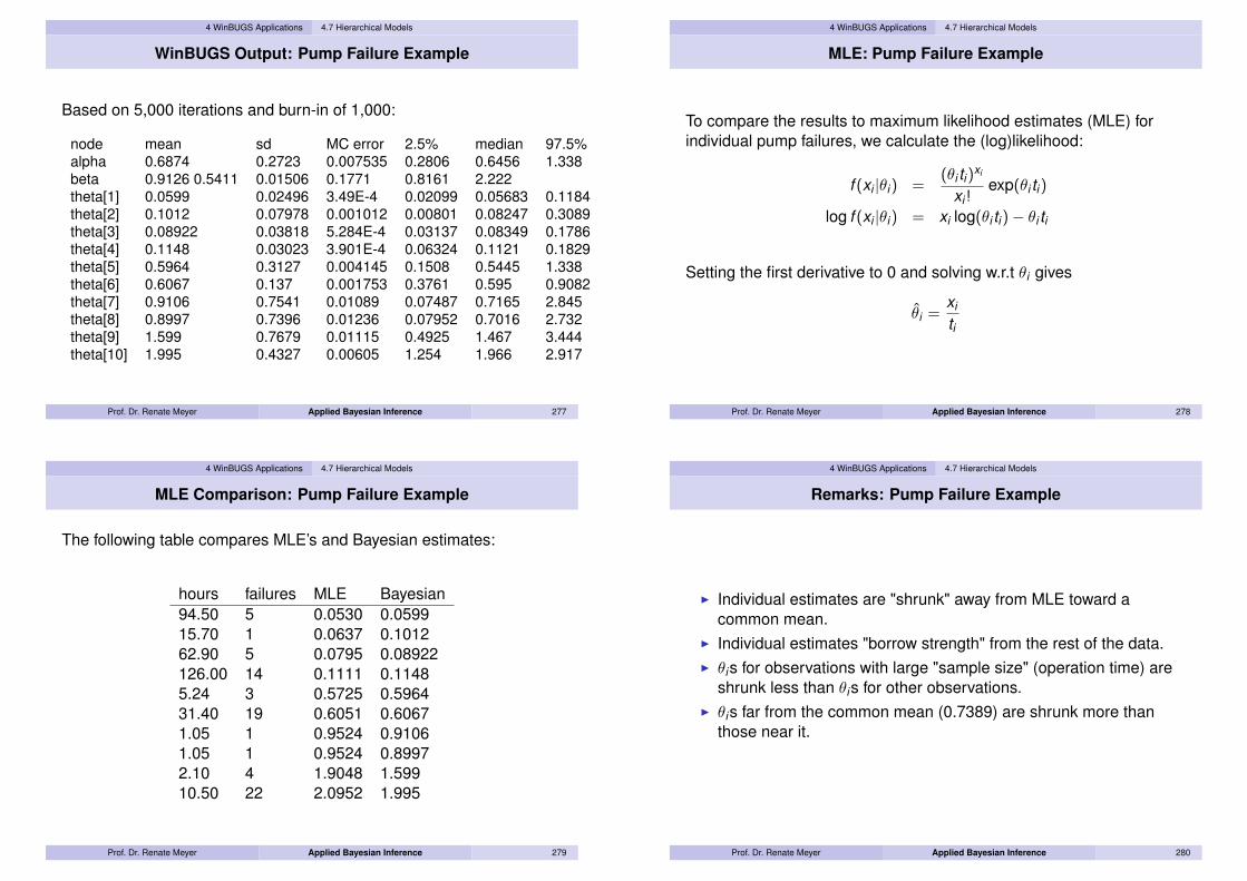
4 WinBUGS Applications 4.7 Hierarchical Models
WinBUGS Output: Pump Failure Example
Based on 5,000 iterations and burn-in of 1,000:
node mean sd MC error 2.5% median 97.5%alpha 0.6874 0.2723 0.007535 0.2806 0.6456 1.338beta 0.9126 0.5411 0.01506 0.1771 0.8161 2.222theta[1] 0.0599 0.02496 3.49E-4 0.02099 0.05683 0.1184theta[2] 0.1012 0.07978 0.001012 0.00801 0.08247 0.3089theta[3] 0.08922 0.03818 5.284E-4 0.03137 0.08349 0.1786theta[4] 0.1148 0.03023 3.901E-4 0.06324 0.1121 0.1829theta[5] 0.5964 0.3127 0.004145 0.1508 0.5445 1.338theta[6] 0.6067 0.137 0.001753 0.3761 0.595 0.9082theta[7] 0.9106 0.7541 0.01089 0.07487 0.7165 2.845theta[8] 0.8997 0.7396 0.01236 0.07952 0.7016 2.732theta[9] 1.599 0.7679 0.01115 0.4925 1.467 3.444theta[10] 1.995 0.4327 0.00605 1.254 1.966 2.917
Prof. Dr. Renate Meyer Applied Bayesian Inference 277
4 WinBUGS Applications 4.7 Hierarchical Models
MLE: Pump Failure Example
To compare the results to maximum likelihood estimates (MLE) forindividual pump failures, we calculate the (log)likelihood:
f (xi |θi) =(θi ti)xi
xi !exp(θi ti)
log f (xi |θi) = xi log(θi ti)− θi ti
Setting the first derivative to 0 and solving w.r.t θi gives
θi =xi
ti
Prof. Dr. Renate Meyer Applied Bayesian Inference 278
4 WinBUGS Applications 4.7 Hierarchical Models
MLE Comparison: Pump Failure Example
The following table compares MLE’s and Bayesian estimates:
hours failures MLE Bayesian94.50 5 0.0530 0.059915.70 1 0.0637 0.101262.90 5 0.0795 0.08922126.00 14 0.1111 0.11485.24 3 0.5725 0.596431.40 19 0.6051 0.60671.05 1 0.9524 0.91061.05 1 0.9524 0.89972.10 4 1.9048 1.59910.50 22 2.0952 1.995
Prof. Dr. Renate Meyer Applied Bayesian Inference 279
4 WinBUGS Applications 4.7 Hierarchical Models
Remarks: Pump Failure Example
I Individual estimates are "shrunk" away from MLE toward acommon mean.
I Individual estimates "borrow strength" from the rest of the data.I θis for observations with large "sample size" (operation time) are
shrunk less than θis for other observations.I θis far from the common mean (0.7389) are shrunk more than
those near it.
Prof. Dr. Renate Meyer Applied Bayesian Inference 280

4 WinBUGS Applications 4.7 Hierarchical Models
Boxplot: Pump Failure Example
[1]
[2][3] [4]
[5]
[6]
[7][8]
[9]
[10]
box plot: theta
0.0
1.0
2.0
3.0
4.0
Figure 18: Boxplots for pump failure rates.
Prof. Dr. Renate Meyer Applied Bayesian Inference 281
4 WinBUGS Applications 4.7 Hierarchical Models
Model Fit Plot: Pump failure Example
model fit: theta
0.0 1.0 2.0 3.0
0.0
1.0
2.0
3.0
4.0
Figure 19: Model fit for pump failure rates.
Prof. Dr. Renate Meyer Applied Bayesian Inference 282
4 WinBUGS Applications 4.7 Hierarchical Models
Prof. Dr. Renate Meyer Applied Bayesian Inference 283
4 WinBUGS Applications 4.7 Hierarchical Models
Prof. Dr. Renate Meyer Applied Bayesian Inference 284

4 WinBUGS Applications 4.8 Survival Analysis
Survival Analysis
Survival Analysis refers to a class of statistical models used to analysethe duration of time until an event of interest (such as death, tumoroccurrence, component failure) occurs. Time-to-event data arise inmany disciplines, including medicine, biology, engineering,epidemiology and economics. Frequentist textbooks include Cox andOakes (1984) and Klein and Moeschberger (1997); a comprehensiveBayesian perspective is given in Ibrahim, Chen and Sinha (2001).
As duration times are non-negative, only non-negative randomvariables can be used to model survival times.
Failure time data are often censored, i.e. incomplete in that one knowsthat a patient survived the study end point, but one does not know theexact time of death.
In survival analysis, we are less interested in the mean of thedistribution but we are interested in the hazard function.
Prof. Dr. Renate Meyer Applied Bayesian Inference 285
4 WinBUGS Applications 4.8 Survival Analysis
Hazard Function
Let T be a continuous nonnegative random variable, representing theduration time until a certain event occurs. Let f (t) denote the pdf andF (t) the cdf of T . Let S(t) = 1− F (t) = P(T ≥ t) be the survivalfunction, which provides the probability of surviving until timepoint t .
Definition 4.6The hazard function is defined as
h(t) = limδt→0
P(t < T ≤ t + δt |T > t)δt
=f (t)S(t)
= −S′(t)S(t)
and can be interpreted as the instantaneous death (or event) rate of anindividual, provided that this person survived until time t . In particular,
h(t)δt is the approximate probability of failure in [t , t + δt), givensurvival up to time t .
Prof. Dr. Renate Meyer Applied Bayesian Inference 286
4 WinBUGS Applications 4.8 Survival Analysis
Hazard Function
Since f (t) = − ddt S(t), Definition 4.6 implies that
h(t) = − ddt
log S(t) (4.1)
Integrating both sides of (4.1), and then exponentiating, yields
S(t) = exp(−∫ t
0h(u)du
). (4.2)
The cumulative hazard, Ht(t) is defined as
H(t) =
∫ t
0h(u)du
so S(t) = exp(−H(t)). Since S(∞) = 0, H(∞) =∞.Prof. Dr. Renate Meyer Applied Bayesian Inference 287
4 WinBUGS Applications 4.8 Survival Analysis
Hazard Function
Thus, the hazard function has the properties
h(t) ≥ 0 and∫ ∞
0h(t)dt =∞.
Finally, it follows from Definition 4.6 and (4.1) that
f (t) = h(t) exp(−∫ t
0h(u)du
). (4.3)
Prof. Dr. Renate Meyer Applied Bayesian Inference 288

4 WinBUGS Applications 4.8 Survival Analysis
Example: Weibull Distribution
Suppose T has pdf
f (t) =
{ργtρ−1 exp(−ρtα), for t > 0, ρ > 0, γ > 0,0, otherwise.
This is a Weibull distribution with parameters (ρ, γ). It follows easilyfrom the equations above, that
I S(t) = exp(−γtρ),I h(t) = γρtρ−1,I H(t) = γtρ.
Prof. Dr. Renate Meyer Applied Bayesian Inference 289
4 WinBUGS Applications 4.8 Survival Analysis
Proportional Hazards Models
The hazard function depends in general on both time and a set ofcovariates. The proportional hazards model (Cox, 1972) separatesthese components by specifying that the hazard at time t for anindividual whose covariate vector is x is given by
h(t ,x) = h0(t) exp{G(x,β)}where h0(t) is called the baseline hazard function and β is a vector ofregression coefficients. The second term is written in exponential formbecause it must be positive.
The ratio of hazards for two individuals is constant over time. Often,the effect on the covariates is assumed to be multiplicative, leading tothe hazard function
h(t ,x) = h0(t) exp(x′β)
where η = x′β is called the linear predictor. Thus the ratio of hazardsfor two individuals depends on the difference between their linearpredictors at any time.
Prof. Dr. Renate Meyer Applied Bayesian Inference 290
4 WinBUGS Applications 4.8 Survival Analysis
Partial Likelihood
Cox’s version (Cox, 1975) of the proportional hazards model issemiparametric as the baseline hazard function h0(t) is not modeledas a parametric function of t .
Assumptions:I n individuals, d have distinct event times, n − d have right
censored survival timesI no ties, ordered survival times: y(1), . . . , y(d)
I Rj = set of individuals who are at risk at time y(j), j th risk set
Then the partial likelihood is:
PL(β) =n∏
i=1
exp(x′(j)β)∑l∈Rj
exp(x′lβ)(4.4)
The partial MLE of β can be obtained by maximizing (4.4) w.r.t. β.Prof. Dr. Renate Meyer Applied Bayesian Inference 291
4 WinBUGS Applications 4.8 Survival Analysis
Likelihood under Censoring
Survival data are often right-censored. An observation is said to beright-censored at c if the exact value of the observation is not knownbut only that it is greater than c.
Let n be number of subjects where individual i has survival time ti andfixed censoring time ci . ti are iid with pdf f (t).The exact survival time ti of an individual will be observed only if ti ≤ ci .Data can be represented by n pairs of random variables (yi , νi) where
yi = min(ti , ci)
and
νi =
{0 if ti ≤ ci ,1 if ti > ci .
Prof. Dr. Renate Meyer Applied Bayesian Inference 292

4 WinBUGS Applications 4.8 Survival Analysis
Likelihood under Censoring
The likelihood function for (β,h0(t)) for right censored data:
L(β,h0(t)|D) ∝n∏
i=1
f (yi)1−νi S(yi)
νi
∝n∏
i=1
h(yi)1−νi S(yi)
1−νi S(yi)νi
∝n∏
i=1
h(yi)1−νi S(yi)
∝n∏
i=1
h(yi)1−νi exp{−H(yi)}
∝n∏
i=1
h0(yi) exp(ηi)]1−νi exp{−exp(ηi)H0(yi)}
where the data D = (n,y,X , ν).Prof. Dr. Renate Meyer Applied Bayesian Inference 293
4 WinBUGS Applications 4.8 Survival Analysis
Likelihood under Censoring
If we assume a parametric model for the baseline hazard, e.g.Weibull(α,1), and define γi = exp(ηi), then the likelihood above is thatof independent censored Weibull(α, γi) distributions.
Prof. Dr. Renate Meyer Applied Bayesian Inference 294
4 WinBUGS Applications 4.8 Survival Analysis
Censoring in WinBUGS
In WinBUGS, right censoring can be implemented using the commandI(a,) (and I(,b) and I(a,b) for left and interval censoring,respectively).
Two variables are required to define the survival times:I the actual survival times t[i] taking NA values for censored
observations andI the censoring times t.cen[i], which take the value 0 when
actual survival times (deaths) are observed.
For example, the likelihood of a Weibull(ρ, γ) distribution with rightcensored data can be expressed as
t[i] dweib(rho,gamma)I(t.cen[i],)
Prof. Dr. Renate Meyer Applied Bayesian Inference 295
4 WinBUGS Applications 4.8 Survival Analysis
Mice Example in WinBUGS
We will now look at the mice example in WinBUGS ExampleVolume 1.
Prof. Dr. Renate Meyer Applied Bayesian Inference 296

4 WinBUGS Applications 4.8 Survival Analysis
MAC AIDS Trial
Here we come back to the analysis of controlled clinical AIDS trialdiscussed in the introduction. Our data arises from a clinical trialcomparing two treatments for Mycobacterium avium complex (MAC), adisease common in late state HIV-infected persons.
11 clinical centers (units) have enrolled a total of 69 patients in thetrial, of which 18 have died. The data have been analysed in Carlinand Hodges (1999) and Cai and Meyer (2011)
I For j = 1, . . . ,ni and i = 1, . . . , k lettij = time to death or censoringxij = treatment indicator for subject j in stratum i
I The next page gives survival times (in half-days) from the MACtreatment trial, where "+" indicates a censored observation
Prof. Dr. Renate Meyer Applied Bayesian Inference 297
4 WinBUGS Applications 4.8 Survival Analysis
Primary Endpoint Data
Unit Treatm. Time Unit Treatm. Time Unit Treatm. TimeA 1 74+ B 2 4+ F 1 6A 2 248 B 1 156+ F 2 16+A 1 272+ F 1 76A 2 244 C 2 20+ F 2 80D 2 20+ E 1 50+ F 2 202D 2 64 E 2 64+ F 1 258+D 2 88 E 2 82 F 1 268+D 2 148+ E 1 186+ F 2 368+D 1 162+ E 1 214+ F 1 380+D 1 184+ E 1 214 F 1 424+D 1 188+ E 2 228+ F 2 428+D 1 198+ E 2 262 F 2 436+D 1 382+D 1 436+G 2 32+ H 2 22+ I 2 8G 1 64+ H 1 22+ I 2 16+G 2 102 H 1 74+ I 2 40G 2 162+ H 1 88+ I 1 120+G 2 182+ H 1 148+ I 1 168+G 1 364+ H 2 162 I 2 174+J 1 18+ K 1 28+ I 1 268+J 1 36+ K 1 70+ I 2 276J 2 160+ K 2 106+ I 1 286+J 2 254 I 1 366
I 2 396+I 2 466+I 1 468+
Prof. Dr. Renate Meyer Applied Bayesian Inference 298
4 WinBUGS Applications 4.8 Survival Analysis
Proportional Hazards Model
With proportional hazards and a Weibull baseline hazard, stratum i ’shazard is
h(tij) = h0(tij)i exp(β0 + β1xij)
= ρi trhoi−1ij exp(β0 + β1xij)
where ρi > 0 and β = (β0, β1).
The ρi allow differing baseline hazards which are increasing if ρi > 1and decreasing if ρi < 1. As the strata may be similar, we model theshape parameters as exchangeable, i.e.
ρiiid∼ Gamma(α, α).
Thus, the mean of the ρi is one, corresponding to a constant baselinehazard and variance 1
α . We put a proper but low informationGamma(3.0, 0.1) prior on α, reflecting a prior guess for the standarddeviation of ρi of 30−1/2 ≈ 0.18 allowing a fairly broad region of valuescentered around one.
Prof. Dr. Renate Meyer Applied Bayesian Inference 299
4 WinBUGS Applications 4.8 Survival Analysis
Proportional Hazards Model
As in the mice example,
µij = exp(β0 + β1xij)
so thatTij ∼Weibull(ρi , µij).
Prof. Dr. Renate Meyer Applied Bayesian Inference 300

4 WinBUGS Applications 4.8 Survival Analysis
Weibull Prop. Hazards: WinBUGS Code
model{for (i in 1 : 69) {
t[i] ~ dweib(rho[unit[i]], mu[i]) I(t.cen[i], )mu[i] <-exp(beta0+beta1*x[i])}
for (k in 1:11){rho[k] ~ dgamma(alpha,alpha)}
alpha ~ dgamma(3.0,0.1)beta0 ~ dnorm(0.0,0.001)beta1 ~ dnorm(0.0,0.001)r <- exp(2.0*beta1)}
Prof. Dr. Renate Meyer Applied Bayesian Inference 301
4 WinBUGS Applications 4.8 Survival Analysis
WinBUGS Output
Based on 10,000 iterations and burn-in of 5,000:
node mean sd MC error 2.5% median 97.5%alpha 48.45 20.12 0.3892 18.47 45.61 95.32beta0 -6.788 0.4114 0.01758 -7.626 -6.78 -6.006beta1 0.5973 0.2805 0.009956 0.06683 0.5894 1.189r 3.887 2.515 0.08594 1.143 3.251 10.78rho[1] 1.028 0.1078 0.002538 0.8111 1.029 1.237rho[2] 0.9848 0.1456 0.003415 0.704 0.9794 1.289rho[3] 0.972 0.1414 0.002471 0.7016 0.9696 1.255rho[4] 0.999 0.1108 0.004363 0.7739 1.0 1.214rho[5] 1.066 0.1024 0.002894 0.8667 1.064 1.273rho[6] 0.9642 0.08855 0.002924 0.7894 0.9654 1.133rho[7] 0.9724 0.1169 0.00354 0.748 0.9709 1.204rho[8] 1.038 0.1273 0.003974 0.7931 1.038 1.296rho[9] 0.9756 0.09325 0.003106 0.7885 0.9763 1.158rho[10] 1.008 0.12 0.002795 0.7667 1.006 1.248rho[11] 0.9616 0.1386 0.003722 0.6873 0.96 1.242
Prof. Dr. Renate Meyer Applied Bayesian Inference 302
4 WinBUGS Applications 4.8 Survival Analysis
WinBUGS Output
I Units A, E, and H have increasing baseline hazard functions(ρi > 0).
I All other units have constant or decreasing baseline hazardfunctions (ρi ≤ 0).
I There is a significant treatment effect:95% CI for β1 does not include 095% CI for r does not include 1
I Posterior mean of the relative risk is closer to frequentist estimater = 3.1 for the unstratified Cox proportional hazards model (cf.Introduction).
Prof. Dr. Renate Meyer Applied Bayesian Inference 303
4 WinBUGS Applications 4.8 Survival Analysis
Prof. Dr. Renate Meyer Applied Bayesian Inference 304

4 WinBUGS Applications 4.9 State-Space Modelling of Time Series
State-Space Modelling of Time Series
State-space models are among the most powerful tools for dynamicmodeling and forecasting of time series and longitudinal data.Overviews can be found in Fahrmeir and Tutz (1994) and Kuensch(2001).Observation equation:
yt = ht (θt ) + vt
gives the conditional distribution of observations yt at time t givenlatent states θt . vt is an error distribution, e.g. N(0, σ2).State equation:
θt = gt (θt−1) + ut
gives the Markovian transition of state θt−1 to θt where ut denotes anerror distribution. The ability to include knowledge of the systembehaviour in the statistical model is largely what makes state-spacemodeling so attractive for biologists, economists, engineers andphysicists.
Prof. Dr. Renate Meyer Applied Bayesian Inference 305
4 WinBUGS Applications 4.9 State-Space Modelling of Time Series
State-Space Modelling of Time Series
ML estimation of unknown parameters and latent states is difficult.
Kalman filter is applicable only for linear Gaussian state-space models.
For nonlinear non-normal state-space models, the likelihood function isintractable.
For nonlinear non-normal state-space models, Carlin et al. (1992)suggested the Gibbs sampler for posterior computation.
In the sequel, we will look at examples of state-space modelsimplemented in WinBUGS.
Prof. Dr. Renate Meyer Applied Bayesian Inference 306
4 WinBUGS Applications 4.9 State-Space Modelling of Time Series
Fisheries Stock Assessment: Data
The data available for stock assessment purposes quite often consistof a time series of annual catches Ct , t = 1, . . . ,N, and relativeabundance indices It , t = 1, . . . ,N, such as research survey catchrates or catch-per-unit-effort (CPUE) indices from commercialfisheries.
For example, the next table gives an historical dataset of catch-effortdata of South Atlantic albacore tuna (Thunnus alalunga) from 1967 to1989. Catch is in thousands of tons and CPUE in (kg/100 hooks).
Prof. Dr. Renate Meyer Applied Bayesian Inference 307
4 WinBUGS Applications 4.9 State-Space Modelling of Time Series
Fisheries Stock Assessment: Data
Yellowfin tuna data from Pella and Tomlinson (1969)
Year (t) Catch (Ct ) CPUE (It )1967 15.9 61.891968 25.7 78.981969 28.5 55.591970 23.7 44.611971 25.0 56.89
......
...1987 37.5 23.361988 25.9 22.361989 25.3 21.91
Prof. Dr. Renate Meyer Applied Bayesian Inference 308

4 WinBUGS Applications 4.9 State-Space Modelling of Time Series
Fisheries Stock Assessment: Objectives
Age-composition data are not available for this stock. This dataset haspreviously been analysed by Polacheck et al. (1993).
Objectives: estimation ofI the size of the stock at the end of 1989,I the maximum surplus production (MSP),I the biomass at which MSP occurs (BMSP),I the optimal effort (EMSP), the level of commercial fishing effort
required to harvest MSP when the stock is at BMSP .When only catch-effort data are available, biomass dynamics modelsare the primary assessment tools for many fisheries (Hilborn andWalters 1992).
Prof. Dr. Renate Meyer Applied Bayesian Inference 309
4 WinBUGS Applications 4.9 State-Space Modelling of Time Series
Fisheries Stock Assessment: Biomass Dynamics
Biomass Dynamics Model
new biomass = old biomass+ growth+ recruitment− natural mortality− catch
The biomass dynamics equations can be written in the form:
Bt = Bt−1 + g(Bt−1)− Ct−1
where Bt , Ct , and g(Bt ) denote biomass at the start of year t , catchduring year t , and the surplus production function, respectively.g(0) = g(K ) = 0, where K is the carrying capacity ( the level of thestock biomass at equilibrium prior to commencement of the fishery).
Prof. Dr. Renate Meyer Applied Bayesian Inference 310
4 WinBUGS Applications 4.9 State-Space Modelling of Time Series
Fisheries Stock Assessment: Surplus Production Model
The Schaefer (1954) form of the surplus production function is
g(Bt−1) = rBt−1
(1− Bt−1
K
).
Substituting this in the biomass dynamics equation gives aparsimonious model describing the annual biomass dynamicstransitions with just the two parameters r , the intrinsic growth rate, andK :
Bt = Bt−1 + rBt−1
(1− Bt−1
K
)− Ct−1. (4.5)
Note that the annual catch is treated as a fixed constant.
Prof. Dr. Renate Meyer Applied Bayesian Inference 311
4 WinBUGS Applications 4.9 State-Space Modelling of Time Series
Fisheries Stock Assessment: Relative Abundance Index
A common, though simplifying assumption is that the relativeabundance index is directly proportional to the biomass, i.e.
It = qBt (4.6)
with catchability parameter q.
For the Schaefer surplus production model, the maximum surplusproduction MSP = rK/4 occurs at BMSP = K/2.When the biomass indices are CPUE’s from commercial fishing, thenthe equation above gives MSP/EMSP = qK/2 and thereby the optimaleffort is EMSP = r/2q.
Prof. Dr. Renate Meyer Applied Bayesian Inference 312

4 WinBUGS Applications 4.9 State-Space Modelling of Time Series
Fisheries Stock Assessment: Process and Observation Error
Polacheck et al. (1993) compare three commonly used statisticaltechniques for fitting the model defined by equations (4.5) and (4.6),process error models, observation error models, and equilibriummodels.None of these is capable of incorporating uncertainty present in bothequations:
I natural variability underlying the annual biomass dynamicstransitions (process error) and
I uncertainty in the observed abundance indices due tomeasurement and sampling error (observation error).
Prof. Dr. Renate Meyer Applied Bayesian Inference 313
4 WinBUGS Applications 4.9 State-Space Modelling of Time Series
Fisheries Stock Assessment: State-Space Model
This is possible, however, using a state-space model.
Equations (4.5) and (4.6) are the deterministic versions of thestochastic state and observation equations.
We assumed log-normal error structures.We used a reparametrization (Pt = Bt/K ) by expressing the annualbiomass as a proportion of carrying capacity as in Millar and Meyer(2000) to speed mixing (i.e. sampling over the support of the posteriordistribution) of the Gibbs sampler.
Prof. Dr. Renate Meyer Applied Bayesian Inference 314
4 WinBUGS Applications 4.9 State-Space Modelling of Time Series
Fisheries Stock Assessment: State-Space Model
State equations:
P1|σ2 = eu1 ,
Pt |Pt−1,K , r , σ2 = (Pt−1 + rPt−1(1− Pt−1)− Ct−1/K ) · eut , t = 2, . . . ,N(4.7)
Observation equations:
It |Pt ,q, τ2 = qKPt · evt , t = 1, . . . ,N, (4.8)
where ut are iid normal with mean 0 and variance σ2, and vt are iidnormal with mean 0 and variance τ2.
Prof. Dr. Renate Meyer Applied Bayesian Inference 315
4 WinBUGS Applications 4.9 State-Space Modelling of Time Series
Fisheries Stock Assessment: Posterior Distribution
A fully Bayesian model consists of the joint prior distribution of allunobservables, here the five parameters, K , r ,q, σ2, τ2, and theunknown states, P1, . . . ,PN ,
and the joint distribution of the observables, here the relativeabundance indices I1, . . . , IN .
We assume that the parameters K , r ,q, σ2, τ2 are independent a priori.By a successive application of Bayes theorem and conditionalindependence of subsequent states, the joint prior density is given by
p(K , r ,q, σ2, τ2,P1, . . . ,PN) = p(K )p(r)p(q)p(σ2)p(τ2)p(P1|σ2)N∏
i=2
p(Pt |Pt−1,K , r , σ2).
Prof. Dr. Renate Meyer Applied Bayesian Inference 316

4 WinBUGS Applications 4.9 State-Space Modelling of Time Series
Fisheries Stock Assessment: Prior Specification
A noninformative prior is chosen for q.Prior distributions for K , r , σ2, τ2 are specified using biologicalknowledge and inferences from related species and stocks asdiscussed in Millar and Meyer (2000):
K ∼ lognormal(µK = 5.04, σK = 0.5162),
r ∼ lognormal(µr = −1.38, σr = 0.51),
p(q) ∝ 1/q,σ2 ∼ inverse-gamma(3.79,0.0102),
τ2 ∼ inverse-gamma(1.71,0.0086).
Prof. Dr. Renate Meyer Applied Bayesian Inference 317
4 WinBUGS Applications 4.9 State-Space Modelling of Time Series
Fisheries Stock Assessment: Likelihood
Because of the conditional independence assumption of the relativeabundance indices given the unobserved states, the samplingdistribution is
p(I1, . . . , IN |K , r ,q, σ2, τ2,P1, . . . ,PN) =N∏
t=1
p(It |Pt ,q, τ2). (4.10)
Then, by Bayes theorem, the joint posterior distribution of theunobservables given the data is
p(K , r ,q, σ2, τ2,P1, . . . ,PN |I1, . . . , IN) ∝ p(K )p(r)p(q)p(σ2)p(τ2)p(P1|σ2)N∏
i=2
p(Pt |Pt−1,K , r , σ2)
N∏t=1
p(It |Pt ,q, τ2)
(4.11)Prof. Dr. Renate Meyer Applied Bayesian Inference 318
4 WinBUGS Applications 4.9 State-Space Modelling of Time Series
Fisheries Stock Assessment: WinBUGS Code
model {# lognormal prior on KK ~ dlnorm(5.042905,3.7603664)I(10,1000)# lognormal prior on rr ~ dlnorm(-1.151293,1.239084233)I(0.005,1.0)# instead of improper (prop. to 1/q) use just proper IGiq ~ dgamma(0.001,0.001)I(0.5,200)q <- 1/iq# inverse gamma on isigma2isigma2 ~ dgamma(a0,b0)sigma2 <- 1/isigma2# inverse gamma on itau2itau2 ~ dgamma(c0,d0)tau2 <- 1/itau2
Prof. Dr. Renate Meyer Applied Bayesian Inference 319
4 WinBUGS Applications 4.9 State-Space Modelling of Time Series
Fisheries Stock Assessment: WinBUGS Code
Pmean[1] <- 0P[1] ~ dlnorm(Pmean[1],isigma2) I(0.05,1.6)for (i in 2:N) {
Pmean[i]<-log(max(P[i-1] + r*P[i-1]*(1-P[i-1]) - C[i-1]/K,0.01))P[i] ~ dlnorm(Pmean[i],isigma2)I(0.05,1.5)}
for (i in 1:N) {Imean[i] <- log(q*K*P[i])I[i] ~ dlnorm(Imean[i],itau2)}
P24 ~ dlnorm(Pmean24, isigma2)I(0.05,1.5)Pmean24<- log(max(P[23] + r*P[23]*(1-P[23]) - C[23]/K,0.01))MSP<- r*K/4B_MSP<- K/2E_MSP<- r/(2*q)}
Prof. Dr. Renate Meyer Applied Bayesian Inference 320

4 WinBUGS Applications 4.9 State-Space Modelling of Time Series
Fisheries Stock Assessment: DAG
for(t IN 2 : N)
C[t-1]
itau2iqK
I[t]Imed[t]
isigma2r
Pmed[t+1]P[t]Pmed[t]P[t-1]
Figure 20: Representation of surplus production model as DAG.
Prof. Dr. Renate Meyer Applied Bayesian Inference 321
4 WinBUGS Applications 4.9 State-Space Modelling of Time Series
Fisheries Stock Assessment: WinBUGS Output
Based on 100,000 iterations and burn-in of 100,000:
node mean sd MC error 2.5% median 97.5%BMSP 135.5 32.44 1.272 87.2 130.2 2121EMSP 0.6154 0.09112 0.001935 0.4346 0.6148 0.8002K 271.0 64.88 2.544 174.4 260.4 424.2MSP 19.52 2.537 0.05968 13.9 19.76 23.94P[1] 1.018 0.05427 8.062E-4 0.919 1.016 1.133P[2] 0.9944 0.07386 0.001368 0.8737 0.986 1.164P[3] 0.8772 0.06548 0.001485 0.7616 0.8726 1.019P[4] 0.7825 0.06205 0.001524 0.6711 0.779 0.9144P[21] 0.4175 0.03452 8.162E-4 0.3545 0.4156 0.491P[22] 0.353 0.03519 9.208E-4 0.292 0.35 0.4296P[23] 0.3271 0.03964 0.00103 0.2573 0.3241 0.4123P24 0.2964 0.04939 0.001221 0.2093 0.2926 0.4028q 0.2486 0.06136 0.002411 0.1449 0.244 0.3777r 0.3088 0.09576 0.003559 0.1416 0.3031 0.5104sigma2 0.003105 0.001912 2.22E-5 0.001132 0.00261 0.008057tau2 0.01225 0.004516 2.778E-5 0.005832 0.01145 0.02327
Prof. Dr. Renate Meyer Applied Bayesian Inference 322
4 WinBUGS Applications 4.9 State-Space Modelling of Time Series
Prof. Dr. Renate Meyer Applied Bayesian Inference 323
4 WinBUGS Applications 4.9 State-Space Modelling of Time Series
Prof. Dr. Renate Meyer Applied Bayesian Inference 324

4 WinBUGS Applications 4.9 State-Space Modelling of Time Series
Example: Stochastic Volatility in Financial Time Series
The stochastic volatility (SV) model introduced by Tauchen and Pitts(1983) is used to describe financial time series. It offers an alternativeto the ARCH-type models of Engle (1982) for the well documentedtime varying volatility exhibited in many financial time series.
The SV model provides a more realistic and flexible modeling offinancial time series than the ARCH-type models, since it essentiallyinvolves two noise processes, one for the observations, and one for thelatent volatilities.
The so called observation errors account for the variability due tomeasurement and sampling errors whereas the process errors assessvariation in the underlying volatility dynamics.
Prof. Dr. Renate Meyer Applied Bayesian Inference 325
4 WinBUGS Applications 4.9 State-Space Modelling of Time Series
Example: Stochastic Volatility in Financial Time Series
Classical parameter estimation for SV models is difficult due to theintractable form of the likelihood function. Recently, a variety offrequentist estimation methods have been proposed for the SV model,including Generalized Method of Moments (Melino and Turnbull(1990), Sorenson (2000)), Quasi-Maximum Likelihood (Harvey et al.,1994), Efficient Method of Moments (Gallant et al., 1997), SimulatedMaximum Likelihood (Danielsson, 1994, and Sandmann andKoopman, 1998), and approximate Maximum Likelihood (Fridman andHarris, 1998).
Bayesian MCMC procedures for the SV model have been suggestedby Jacquier et al. (1994), Shephard and Pitt (1997), Kim et al. (1998)and Meyer and Yu (2000). Here we demonstrate the implementation ofthe Gibbs sampler in WinBUGS.
Prof. Dr. Renate Meyer Applied Bayesian Inference 326
4 WinBUGS Applications 4.9 State-Space Modelling of Time Series
Stochastic Volatility: Data
The data consist of a time series of daily Pound/Dollar exchange rates{xt} from 01/10/81 to 28/6/85. The series of interest are the dailymean-corrected returns, {yt}, given by the transformationyt = log xt − log xt−1 − 1
n∑n
i=1(log xi − log xi−1), t = 1, . . . ,n.
returns.dat
-0.3202213630797821.46071929942995-0.4086296198109471.060960273866851.712889207631630.404314365893326-0.905699012715806...2.22371628398118
Prof. Dr. Renate Meyer Applied Bayesian Inference 327
4 WinBUGS Applications 4.9 State-Space Modelling of Time Series
Stochastic Volatility: State-Space Model
The SV model used for analyzing these data can be written in the formof a nonlinear state-space model:
Observation equations:
yt |θt = exp(
12θt
)ut , ut
iid∼ N(0,1), t = 1, . . . ,n. (4.12)
State equations:
θt |θt−1, µ, φ, τ2 = µ+ φ(θt−1 − µ) + vt , vt
iid∼ N(0, τ2), t = 1, . . . ,n,(4.13)
with θ0 ∼ N(µ, τ2).
Prof. Dr. Renate Meyer Applied Bayesian Inference 328

4 WinBUGS Applications 4.9 State-Space Modelling of Time Series
Stochastic Volatility: Parameters
I θt determines the amount of volatility on day t ,I the value of φ, −1 < φ < 1, measures the autocorrelation present
in the logged squared data; thus φ can be interpreted as thepersistence in the volatility, and
I the constant scaling factor β = exp(µ/2) as the modal volatility,and
I τ as the volatility of log-volatilities.
Prof. Dr. Renate Meyer Applied Bayesian Inference 329
4 WinBUGS Applications 4.9 State-Space Modelling of Time Series
Stochastic Volatility: Prior Specification
By successive conditioning, the joint prior density is
p(µ, φ, τ2, θ0, θ1, . . . , θn) = p(µ, φ, τ2)p(θ0|µ, τ2)n∏
t=1
p(θt |θt−1, µ, φ, τ2).
(4.14)
I We employ a slightly informative prior for µ, µ ∼ N(0,10).I We set φ = 2φ∗ − 1 and specify a Beta(α, β) prior for φ∗ withα = 20 and β = 1.5 which gives a prior mean for φ of 0.86.
I A conjugate inverse-gamma prior is chosen for τ2, i.e.τ2 ∼ IG(2.5,0.025) which gives a prior mean of 0.0167 and priorstandard deviation of 0.0236.
Prof. Dr. Renate Meyer Applied Bayesian Inference 330
4 WinBUGS Applications 4.9 State-Space Modelling of Time Series
Stochastic Volatility: Likelihood
The likelihood p(y1, . . . , yn|µ, φ, τ2, θ0, . . . , θn) is specified by theobservation equations (4.12) and the conditional independenceassumption:
p(y1, . . . , yn|µ, φ, τ2, θ0, . . . , θn) =n∏
t=1
p(yt |θt ). (4.15)
Prof. Dr. Renate Meyer Applied Bayesian Inference 331
4 WinBUGS Applications 4.9 State-Space Modelling of Time Series
Stochastic Volatility: Posterior Distribution
Then, by Bayes’ theorem, the joint posterior distribution of theunobservables given the data is proportional to the prior timeslikelihood, i.e.
p(µ, φ, τ2, θ0, . . . , θn|y1, . . . , yn) ∝ p(µ)p(φ)p(τ2)p(θ0|µ, τ2)∏nt=1 p(θt |θt−1, µ, φ, τ
2)×∏nt=1 p(yt |θt ).
(4.16)
Prof. Dr. Renate Meyer Applied Bayesian Inference 332
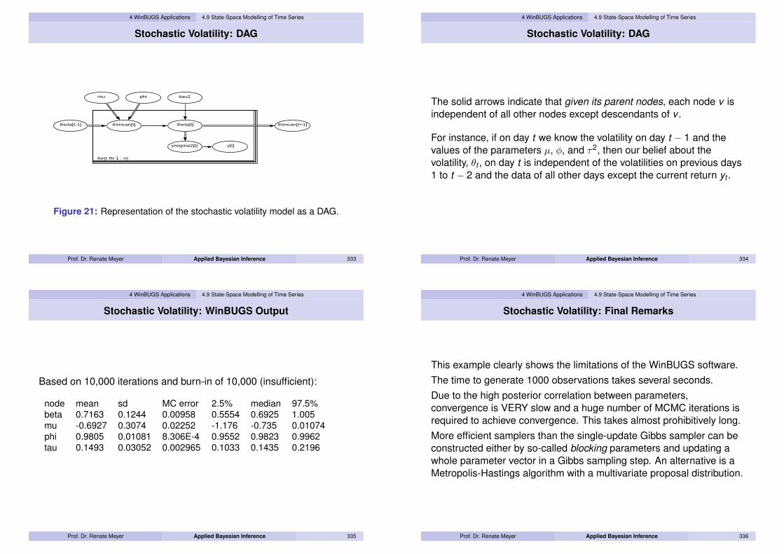
4 WinBUGS Applications 4.9 State-Space Modelling of Time Series
Stochastic Volatility: DAG
for(t IN 1 : n)
mu
y[t]yisigma2[t]
itau2phi
thmean[t+1]theta[t]thmean[t]theta[t-1]
Figure 21: Representation of the stochastic volatility model as a DAG.
Prof. Dr. Renate Meyer Applied Bayesian Inference 333
4 WinBUGS Applications 4.9 State-Space Modelling of Time Series
Stochastic Volatility: DAG
The solid arrows indicate that given its parent nodes, each node v isindependent of all other nodes except descendants of v .
For instance, if on day t we know the volatility on day t − 1 and thevalues of the parameters µ, φ, and τ2, then our belief about thevolatility, θt , on day t is independent of the volatilities on previous days1 to t − 2 and the data of all other days except the current return yt .
Prof. Dr. Renate Meyer Applied Bayesian Inference 334
4 WinBUGS Applications 4.9 State-Space Modelling of Time Series
Stochastic Volatility: WinBUGS Output
Based on 10,000 iterations and burn-in of 10,000 (insufficient):
node mean sd MC error 2.5% median 97.5%beta 0.7163 0.1244 0.00958 0.5554 0.6925 1.005mu -0.6927 0.3074 0.02252 -1.176 -0.735 0.01074phi 0.9805 0.01081 8.306E-4 0.9552 0.9823 0.9962tau 0.1493 0.03052 0.002965 0.1033 0.1435 0.2196
Prof. Dr. Renate Meyer Applied Bayesian Inference 335
4 WinBUGS Applications 4.9 State-Space Modelling of Time Series
Stochastic Volatility: Final Remarks
This example clearly shows the limitations of the WinBUGS software.The time to generate 1000 observations takes several seconds.Due to the high posterior correlation between parameters,convergence is VERY slow and a huge number of MCMC iterations isrequired to achieve convergence. This takes almost prohibitively long.More efficient samplers than the single-update Gibbs sampler can beconstructed either by so-called blocking parameters and updating awhole parameter vector in a Gibbs sampling step. An alternative is aMetropolis-Hastings algorithm with a multivariate proposal distribution.
Prof. Dr. Renate Meyer Applied Bayesian Inference 336

4 WinBUGS Applications 4.10 Copulas
Copulas
The study of copulas and their applications in statistics is a rathermodern phenomenon, although the concept goes back to Sklar (1959),but interest in copulas has been growing over the last 15 years.
What are copulas?
The word copula is a Latin noun that means "a link, tie, bond".
In statistics, copulas are functions that join or "couple" multivariatedistribution functions to their one-dimensional marginal distributionfunctions.
Or: Copulas are multivariate distribution functions whoseone-dimensional margins are uniform on the interval (0,1).
An extensive theoretical discussion of copulas can be found in Nelsen(2006).
Prof. Dr. Renate Meyer Applied Bayesian Inference 337
4 WinBUGS Applications 4.10 Copulas
Applications of Copulas
Copulas are used toI study scale-free measures of dependenceI construct families of bivariate/multivariate distributions (as
alternatives to the multivariate normal, where the normaldistribution does not provide an adequate approximation to manydatasets, e.g. lifetime random variables and long-tailed claimvariables)
Main applications:I in financial risk assessment and actuarial analysis – some believe
the methodology of applying the Gaussian copula to creditderivatives to be one of the reasons behind the global financialcrisis of 2008-2009,
I in engineering for reliability studiesI in biostatistics/epidemiology to model joint survival times of groups
of individuals, e.g. husband and wife, twins, father and son, etc.Prof. Dr. Renate Meyer Applied Bayesian Inference 338
4 WinBUGS Applications 4.10 Copulas
Definition of a Copula
Definition 4.7A copula C(u1, . . . ,ud ) is a multivariate distribution function on the unithypercube [0,1]d with univariate marginal distributions that are alluniform on the interval [0,1], i.e.
C(u1, . . . ,ud ) = P(U1 ≤ u1, . . . ,Ud ≤ ud )
where Ui ∼ Uniform(0,1) for i = 1, . . . ,d .
For ease of notation, we assume from now on that d = 2.
Prof. Dr. Renate Meyer Applied Bayesian Inference 339
4 WinBUGS Applications 4.10 Copulas
Sklar’s Theorem (1959)
Theorem 4.8Let F be a joint distribution function with margins F1 and F2. Thenthere exists a copula C such that for all x1, x2 ∈ IR
F (x1, x2) = C (F1(x1),F2(x2)) . (4.17)
If F1 and F2 are continuous, then C is unique.Conversely, if C is a copula and F1 and F2 are distribution functions,then the function F defined by (4.17) is a joint distribution function withmargins F1 and F2.
Prof. Dr. Renate Meyer Applied Bayesian Inference 340

4 WinBUGS Applications 4.10 Copulas
Copula Density
By differentiation, it is easy to show that the density function of abivariate distribution F (x1, x2) = C (F1(x1),F2(x2)) with marginaldensities f1 and f2 is given by
f (x1, x2) = c(F1(x1),F2(x2))f1(x1)f2(x2) (4.18)
where c denotes the copula density of C, i.e.
c(u1,u2) =∂2
∂u1∂u2C(u1,u2)
.
Prof. Dr. Renate Meyer Applied Bayesian Inference 341
4 WinBUGS Applications 4.10 Copulas
Some Copula Families
Clayton Copula
C(u, v) =(max
(u−α + v−α − 1,0
))−1/αα ∈ [−1,∞)\{0}
Frank Copula
C(u, v) = −1α
log(
1 +(e−αu − 1)(e−αv − 1)
e−α − 1
)α ∈ (−∞,∞)\{0}
Gumbel Copula
C(u, v) = uv exp(−α log u log v) α ∈ (0,1]
Gaussian Copula
C(u, v) = Φρ
(Φ−1(u),Φ−1(v)
)where Φρ is the standard bivariate normal distribution function withcorrelation ρ, and Φ is the standard normal distribution function.
Prof. Dr. Renate Meyer Applied Bayesian Inference 342
4 WinBUGS Applications 4.10 Copulas
Dependance Measure: Concordance
Informally, a pair of rv’s are concordant if "large" values of one tend tobe associated with "large" values of the other and "small" values of onewith "small" values of the other.
Two observations (xi , yi) and (xj , yj) of a random vector (X ,Y ) areconcordant (discordant) if
I xi < xj and yi < yj , or if xi > xj and yi > yj(xi < xj and yi > yj , or if xi > xj and yi < yj )
I or equivalently:(xi − xj)(yi − yj) > 0((xi − xj)(yi − yj) < 0)
Prof. Dr. Renate Meyer Applied Bayesian Inference 343
4 WinBUGS Applications 4.10 Copulas
Dependance Measure: Kendall’s tau
The sample version of Kendall’s tau is defined in terms of concordanceas follows:Let (xi , yi), i = 1, . . . ,n denote a random sample of n observations of
(X ,Y ). There are(
n2
)distinct pairs (xi , yi) and (xj , yj) of
observations in the sample, and each pair is either concordant ordiscordant. Let c denote the number of concordant pairs and d thenumber of discordant pairs. Then Kendall’s tau is defined as
τ =c − dc + d
= (c − d)/
(n2
).
The population version of Kendall’s tau is defined as the probability ofconcordance minus the probability of discordance:
τ = P[(X1 − X2)(Y1 − Y2) > 0]− P[(X1 − X2)(Y1 − Y2) < 0]
Prof. Dr. Renate Meyer Applied Bayesian Inference 344

4 WinBUGS Applications 4.10 Copulas
Relationship: Kendall’s tau and copula parameter
We have the following functional relationships between Kendall’s tauand the parameters of the copula families above:
Clayton τ = 1− 22 + α
Frank τ = 1− 4α
(1− 1
α
∫ α
0
tet − 1
dt)
Gumbel τ = 1− α−1
Gauss τ =2π
arcsin(α)
Prof. Dr. Renate Meyer Applied Bayesian Inference 345
4 WinBUGS Applications 4.10 Copulas
Parameter Estimation
Flexible multivariate distributions can be constructed withpre-specified, discrete and/or continuous marginal distributions andcopula function that represents the desired dependence structure. Thejoint distribution is usually estimated by a standard two-step procedure
I the marginals are approximated by their empirical distribution orparameters of the marginals are estimated via ML
I the parameters in the copula function are estimated by maximumlikelihood conditional on the parameter estimates in the first step.
Here, we propose to estimate jointly all parameters of marginaldistributions and copula using a Bayesian approach implemented inWinBUGS as in Kelly (2007).
Prof. Dr. Renate Meyer Applied Bayesian Inference 346
4 WinBUGS Applications 4.10 Copulas
Simulation Study
We use the copula package in R to simulate N = 500 bivariate failuretimes from a Clayton copula with Exponential(λi ) marginal distributionsand a Kendall’s tau value of 0.8 (as a measure for the associationbetween the failure times). The rates for the marginal distributions areλ1 = λ2 = 0.0001.
We use R2WinBUGS to sample from the posterior distribution of theunknown parameters. We use a Jeffreys prior for the rates of theExponential distributions (i.e. approximately Jeffreys withλi ∼ Gamma(0.001,0.001) and we assume a Uniform(0,100) prior forα (based for instance on a priori information that the associationbetween failure times is positive and won’t exceed 0.98).
To specify the likelihood, we need to calculate the density of themultivariate distribution first using (4.18). Exercise!
Prof. Dr. Renate Meyer Applied Bayesian Inference 347
4 WinBUGS Applications 4.10 Copulas
Simulation Study: R2WinBUGS Code
library(copula)library(R2WinBUGS)p <- 2 # copula dimensiontau <- 0.8 # value of Kendall’s taualpha<-2*tau/(1-tau) #relationship between tau and alphac.clayton<-archmCopula(family="clayton",dim=p,param=alpha)
# Marginals are exponential lambda1 and lambda2lambda1 <- 0.0001lambda2 <- 0.0001distr.clayton<-mvdc(c.clayton, margins=rep("exp",p),
paramMargins = list(list(rate=lambda1),list(rate=lambda2)))
# Draw a random sample of size NN <- 500w <- rmvdc(distr.clayton, N)
Prof. Dr. Renate Meyer Applied Bayesian Inference 348

4 WinBUGS Applications 4.10 Copulas
Simulation Study
●
●
●
●
●
●●
●
●
●
●
●
●●
●
●
●
●
●
●●
●●
●
●●
●
●
●
●●
●
●
●●
●
●
●
●
●
●●
●
●
●
●
●
●●
●
●●
●
●
●●
●
●
●●●
●
●
●
●●
●
●
●
●
●
●
●
●●
●
●
●
●
●
●
●
●●
●
● ●
●
●
●●
●
●●
●
●
●
●
●●
●
● ●
●●
●
●●
●
●
●●
●
●
●
●●●
●
● ●
●
●
●
●
●
●
●●
● ●
●
●
●
●
●●
●
●●
●
●
●●
●
●
●
●
●
●
●
●
●
●●●
●
●
●
●
●
●
●●
● ●●
●
●
●
●
●●
●●
●
●
●
●
●
●
●
●
●
●
●
●
●
●
●
●
●
●●●
●
●
●●
●
●
●
●
●
●
●
●
●
●
●
●●
●
●
●
●
●
●
●
●
●
●
●
●●
●
●
●●
●
●
●●
●
●
●
●
●
●
●
●●
●●
●
●
●
●
●
●
●
●
●
●
●
●
●
●●
●
●
●
●
●
●
●
●
●
●
●
●
●●
●
●
●
●
●
●
●
●
●
●
●
●
●
●
●
●
● ●
●
●
●
●
●
●
●
●
●
●●
●●
●
●
●
●
●
●
●
●●
●
●
●●
●
●
●
●
●
●●
●●
●
●
●
●
●
●
●
●
●
●
●●
●
●
●
●●
●
●
●
●
●
●
●
●
●
●
●
●●
●●
●●
●
●●
●
●
●
●
●
●
●
●
●
●
●
●
●
●●●
●●
●
●
●
●
●
●
●
●
●
●
●
●●
●
●
●
●
●
●
●
●
●
●
●
●
●
●●
●
●●
●
●
●
●
●
●
●
●
●
●
●
●
●●
●●
●
●
●
●
●
●
●
●●
●
●
●
●●
●
●
●●
●
●
●
●
●
●
●
●
●
●
●
●
●●
●
●
●
●
●
●
●
●●
●
●●
●
●
●
●
●
●
●
●
●
● ●
●
●
●
●●
●
●
● ●
●
● ●
●
●
●
●●
0 10000 20000 30000 40000 50000 60000
010
000
2000
030
000
4000
050
000
6000
070
000
w[, 1]
w[, 2
]
Figure 22: Scatterplot of 500 simulated values from Clayton copula withExp(0.0001) marginals.
Prof. Dr. Renate Meyer Applied Bayesian Inference 349
4 WinBUGS Applications 4.10 Copulas
Implementation in WinBUGS: Zeros Trick
If we want to implement parameter estimation of this copula model inWinBUGS, we face a problem as copula distributions are not includedin the list of standard distributions implemented in WinBUGS.
Fortunately, we can use the so-called zeros trick to specify a newsampling distribution. An observation yi with new sampling distributionf (yi |θ) contributes a likelihood term L(i) = f (yi |θ). Let l(i) = log L(i),then the model likelihood can be written as
f (y1, . . . , yn|θ) =n∏
i=1
f (yi |θ) =n∏
i=1
el(i)
=n∏
i=1
−l(i)0
0!e−(−l(i))
i.e. the product of densities of Poisson random variables withmean= −l(i) and all observations equal to zero.
Prof. Dr. Renate Meyer Applied Bayesian Inference 350
4 WinBUGS Applications 4.10 Copulas
Implementation in WinBUGS: Zeros Trick
To ensure that the Poisson means are all positive, we may have to adda positive constant C to each −l(i). This is equivalent to multiplyingthe likelihood by a constant term e−nC . With this approach, the originallikelihood can be written as the product of Poisson likelihoods withobservations all equal to zero:
f (y|θ) =n∏
i=1
−(l(i) + C)0
0!e−(−l(i)+C) =
n∏i=1
fPoisson(0| − l(i) + C)
Generic WinBUGS code:
C <- 10000for (i in 1:n){
zeros[i]<-0zeros[i]~ dpois(zeros.mean[i])zeros.mean[i]<- -l[i]+Cl[i]<- ...#expression of log-likelihood for obs. i
}Prof. Dr. Renate Meyer Applied Bayesian Inference 351
4 WinBUGS Applications 4.10 Copulas
Implementation in WinBUGS: Ones Trick
As an alternative to the zeros trick, the Bernoulli distribution can beused. The likelihood can be written as
f (y1, . . . , yn|θ) =n∏
i=1
(el(i))1 (
1− el(i))0
=n∏
i=1
fBernoulli(1|el(i))
i.e. the product of Bernoulli densities with success probability el(i) andall observations equal to 1.
Prof. Dr. Renate Meyer Applied Bayesian Inference 352
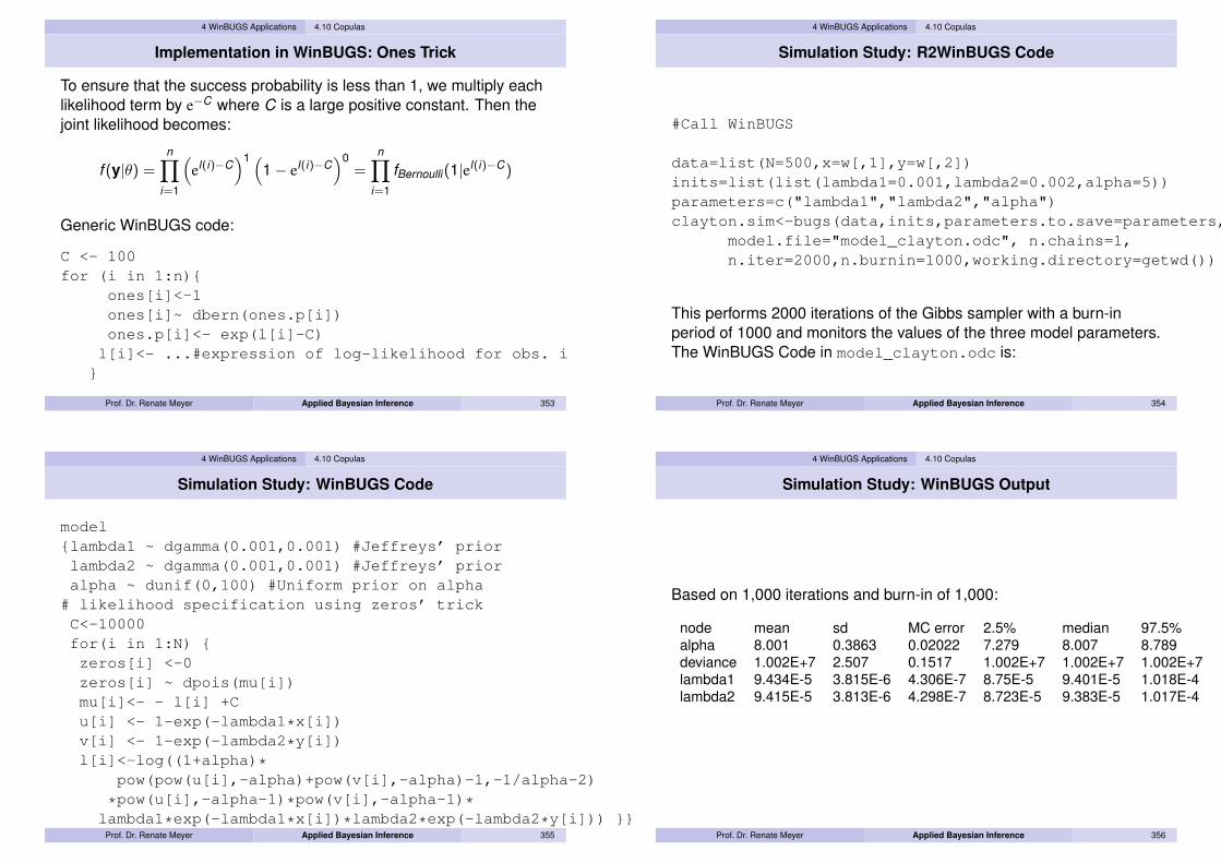
4 WinBUGS Applications 4.10 Copulas
Implementation in WinBUGS: Ones Trick
To ensure that the success probability is less than 1, we multiply eachlikelihood term by e−C where C is a large positive constant. Then thejoint likelihood becomes:
f (y|θ) =n∏
i=1
(el(i)−C
)1 (1− el(i)−C
)0=
n∏i=1
fBernoulli(1|el(i)−C)
Generic WinBUGS code:
C <- 100for (i in 1:n){
ones[i]<-1ones[i]~ dbern(ones.p[i])ones.p[i]<- exp(l[i]-C)l[i]<- ...#expression of log-likelihood for obs. i
}
Prof. Dr. Renate Meyer Applied Bayesian Inference 353
4 WinBUGS Applications 4.10 Copulas
Simulation Study: R2WinBUGS Code
#Call WinBUGS
data=list(N=500,x=w[,1],y=w[,2])inits=list(list(lambda1=0.001,lambda2=0.002,alpha=5))parameters=c("lambda1","lambda2","alpha")clayton.sim<-bugs(data,inits,parameters.to.save=parameters,
model.file="model_clayton.odc", n.chains=1,n.iter=2000,n.burnin=1000,working.directory=getwd())
This performs 2000 iterations of the Gibbs sampler with a burn-inperiod of 1000 and monitors the values of the three model parameters.The WinBUGS Code in model_clayton.odc is:
Prof. Dr. Renate Meyer Applied Bayesian Inference 354
4 WinBUGS Applications 4.10 Copulas
Simulation Study: WinBUGS Code
model{lambda1 ~ dgamma(0.001,0.001) #Jeffreys’ priorlambda2 ~ dgamma(0.001,0.001) #Jeffreys’ prioralpha ~ dunif(0,100) #Uniform prior on alpha
# likelihood specification using zeros’ trickC<-10000for(i in 1:N) {zeros[i] <-0zeros[i] ~ dpois(mu[i])mu[i]<- - l[i] +Cu[i] <- 1-exp(-lambda1*x[i])v[i] <- 1-exp(-lambda2*y[i])l[i]<-log((1+alpha)*
pow(pow(u[i],-alpha)+pow(v[i],-alpha)-1,-1/alpha-2)
*pow(u[i],-alpha-1)*pow(v[i],-alpha-1)*lambda1*exp(-lambda1*x[i])*lambda2*exp(-lambda2*y[i])) }}
Prof. Dr. Renate Meyer Applied Bayesian Inference 355
4 WinBUGS Applications 4.10 Copulas
Simulation Study: WinBUGS Output
Based on 1,000 iterations and burn-in of 1,000:
node mean sd MC error 2.5% median 97.5%alpha 8.001 0.3863 0.02022 7.279 8.007 8.789deviance 1.002E+7 2.507 0.1517 1.002E+7 1.002E+7 1.002E+7lambda1 9.434E-5 3.815E-6 4.306E-7 8.75E-5 9.401E-5 1.018E-4lambda2 9.415E-5 3.813E-6 4.298E-7 8.723E-5 9.383E-5 1.017E-4
Prof. Dr. Renate Meyer Applied Bayesian Inference 356

5 References
References I
I Albert, J.H. (2007), Bayesian Computation with R, Springer, NewYork.
I Aitkin, M. (1997), The calibration of P-values, posterior Bayesfactors and the AIC from the posterior distribution of the likelihood,Statistics and Computing 7: 253:272.
I Aitkin, M. (2010), Statistical Inference, An IntegratedBayesian/Likelihood Approach, Chapman& Hall, Cambridge, UK.
I Bellhouse, D.R. (2004), The Reverend Thomas Bayes, FRS: ABiography to Celebrate the Tercentenary of his Birth, StatisticalScience 19, 3-43.
I Berger, J.O. and Wolpert, R.L. (1988) The Likelihood Principle,Hayward, CA.
I Bernardo, J. and Smith, A. (1994) Bayesian Theory, Wiley,Chichester, UK.
Prof. Dr. Renate Meyer Applied Bayesian Inference 357
5 References
References II
I Bolstad, W.M. (2004) Introduction to Bayesian Statistics, JohnWiley& Sons.
I Borel E. (1921), La Theorie du jeu et les Equations Integrales aNoyau Symetrique, Comptes Rendus de L’Academie desSciences 173 1304-13-8.
I Cai, B., Meyer, R. (2011) Bayesian semiparametric modeling ofsurvival data based on mixtures of B-spline distributions,Computational Statistics and Data Analysis to appear.
I Carlin, B.P., Polson, N.G., and Stoffer, D.S. (1992). A Monte Carloapproach to nonnormal and nonlinear state-space modeling. J.Amer. Statist. Assoc. 87, 493–500.
I Carlin, B.P. and Louis, Th.A. (2008) Bayesian Methods for DataAnalysis, Chapman & Hall.
Prof. Dr. Renate Meyer Applied Bayesian Inference 358
5 References
References III
I Carlin, B.P. and Hodges, (1999), Hierarchical ProportionalHazards Regression Models for Highly Stratified Data, Biometrics55, 1162-1170.
I Cox, D.R. (1972), Regression models and life tables, Journal ofthe Royal Statistical Society B 34, 187-220.
I Cox, D.R. (1975), Partial Likelihood, Biometrika 62, 269-276.I Cox, D.R. and Oakes, D. (1984) Analysis of Survival Data.
London: Chapman& Hall.I Dempster, A.P. (1974), The direct use of likelihood for significance
testing, in (Barndorff-Nielsen et al, eds.) Proc. of the Conferenceon the Foundational Questions of Statistical Inference,335-352,Reprinted in Statistics and Computing 7, 247-252 (1997).
I Dey, D., Ghosh, S. and Mallick, B. (2000), Generalized LinerModels: A Bayesian Perspective, Marcel Dekker, New York.
Prof. Dr. Renate Meyer Applied Bayesian Inference 359
5 References
References IV
I Efron, B. (2005), Bayesians, Frequentists, and Scientists, Journalof the American Statistical Association 100.
I Fahrmeir, L. and Tutz, G. (2001), Multivariate Statistical ModellingBased on Generalized Linear Models, Springer Series inStatistics, Springer Verlag, New York.
I Fisher, R.A. (1922), On the interpretation of chi-square fromcontingency tables and the calculation of p, Journal of the RoyalStatistical Society B, 85, 87-94.
I Gelfand, A., Dey, D., Chang, H. (1992), Model determination usingpredictive distributions with implementation via sampling-basedmethods, in (Bernardo et al. eds) Bayesian Statistics 4, OxfordUniversity Press, 407-425.
I Gelman, A., Carlin, J., Stern, H., Rubin, D. (2004), Bayesian DataAnalysis, Texts in Statistical Science, 2nd ed., Chapman& Hall,London.
Prof. Dr. Renate Meyer Applied Bayesian Inference 360

5 References
References V
I Gelman, A. and Meng, X.L. (1996), Model Checking and modelimprovement, in (Gilks et al, eds) Markov Chain Monte Carlo inPractice, Chapman& Hall, UK, 189-201.
I Geman, S. and Geman, D. (1984), Stochastic relaxation, Gibbsdistributions and the Bayesian restoration of images, IEEEtransactions on Pattern Analysis and Machine Intelligence 6,721-741.
I George, E.I., Makov, U.E. and Smith, A.F.M. (1993), ConjugateLikelihood Distributions, Scandinavian Journal of Statistics, 20,147-156.
I Gilks, W., Richardson, S. and Spiegelhalter, D. (1996), MarkovChain Monte Carlo in Practice, Chapman& Hall, Cambridge, UK.
I Ibrahim, J.G., Chen, M-H., Sinha, D. (2001) Bayesian SurvivalAnalysis. Springer, New York.
Prof. Dr. Renate Meyer Applied Bayesian Inference 361
5 References
References VI
I Jeffreys, H. (1939) Theory of Probability, Oxford University Press,Oxford.
I Jeffresy, H. (1961) Theory of Probability, 3rd edition, OxfordUniversity Press, Oxford.
I Kelly, D.L. (2007), Using Copulas to Model Dependence inSimulation Risk Assessment, Proceedings of InternationalMechanical Engineering Congress and Exposition,IMECE2007-41284.
I Keynes, J.M. (1922) A Treatise on Probability, Volume 8, StMartin’s.
I Klein, J.P. and Moeschberger, M.L. (1997), Survival Analysis, NewYork: Springer.
I Kuensch, H.R. (2001), State space and hidden Markov models, In:Barndorff-Nielsen et al. (Ed.), Complex stochastic systems,Chapman & Hall, London, 109–174.
Prof. Dr. Renate Meyer Applied Bayesian Inference 362
5 References
References VII
I Lawless J.F. (1982) Statistical Models and Methods for Life TimeData. New York, Wiley.
I McCullagh, P. and Nelder, J. (1989), Generalized Linear Models,Chapman& Hall, Cambridge, UK.
I McCarthy, M.A. (2007) Bayesian Methods for Ecology, CambridgeUniversity Press, 2007.
I Meyer, R. and J. Yu (2000), BUGS for a Bayesian analysis ofstochastic volatility models. Econometrics Journal 3, 198-215.
I Millar, R.B. and Meyer R. (2000), State-Space Modeling ofNon-Linear Fisheries Biomass Dynamics Using the GibbsSampler. Applied Statistics, 49, 327-342.
I Nelsen, R.B. (2006) An Introduction to Copulas, Springer, NewYork.
Prof. Dr. Renate Meyer Applied Bayesian Inference 363
5 References
References VIII
I Ntzoufras, I. (2009) Bayesian Modeling Using WinBUGS, JohnWiley& Sons, Inc.
I Raiffa, H. and Schlaiffer, R. Applied Statistical Decision Theory,Cambridge, MIT Press.
I Ramsay, F.P. (1926), Truth and Probability, Publised in 1931 asFoundations of Mathematics and Other Logical Essays Ch. VII,156-198.
I Rubin, D.B. (1984), Bayesianly justifiable and relevant frequencycalculations for the applied statistician, Annals of Statistics 12,1151-1172.
I Sklar, A. 91959), Fonctions de repartition a n dimensions e leursmarges. Publ. Inst. Stat. Univ. Paris 8, 229-231.
I Spiegelhalter, D.J., Best, N.G., Carlin, B.P., van der Linde, A.(2002), Bayesian measures of model complexity and model fit.Journal of the Royal Statistical Society B 64, 583-639.
Prof. Dr. Renate Meyer Applied Bayesian Inference 364