Applications of Synchronous Circuits(Class 10.2 – 3/28/2013)

CSE 2441 – Introduction to Digital LogicSpring 2013

Instructor – Bill Carroll, Professor of CSE

Today’s Topics

• FSM application examples– Sequence recognizer– Code converter– Controller

• Synchronous circuit minimization– State reduction– State assignment

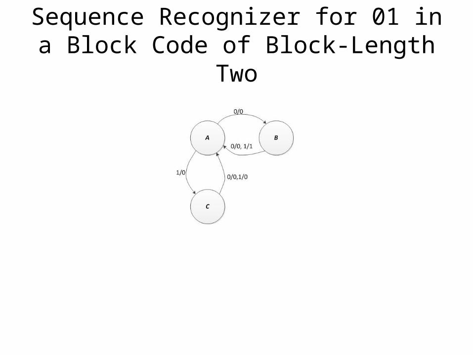
Sequence Recognizer for 01 in a Block Code of Block-Length Two

Test Your Understanding

Design a realization of the block 01 recognizer.

Use the following state assignment and JK flip flops.A: 00, B: 01, C: 10

Test Your Understanding – Self-Check

PS

x

0 1

A B/0 C/0

B A/0 A/1

C A/0 A/0

NS/z

y1y2

x

0 1

00 01/0 10/0

01 00/0 00/1

10 00/0 00/0

Y1Y2/z

y1y2

x

0 1

00 0 0

01 0 1

11 d d

10 0 0

z = xy2

y1y2

x

0 1

00 0 1

01 0 0

11 d d

10 d d

J1

y1y2

x

0 1

00 d d

01 d d

11 d d

10 1 1

K1

y1y2

x

0 1

00 1 0

01 d d

11 d d

10 0 0

J2

y1y2

x

0 1

00 d d

01 1 1

11 d d

10 d d

K2

State Table Transition/Output Table Output K-map

Excitation K-maps

J1 = xy2’ K1 = 1 or y1 J2 = x’y1’ K2 = 1 or y2

Test Your Understanding – Self-Check

Design a Recognizer for the Sequence 1111Example 8.11

Figure 8.29

Note: This solution assumes non-block sequences and allows overlap.

How would the solution change for block sequences and no overlap?

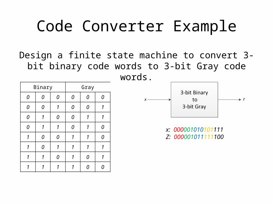
Code Converter Example

Design a finite state machine to convert 3-bit binary code words to 3-bit Gray code words.

Binary Gray

0 0 0 0 0 0

0 0 1 0 0 1

0 1 0 0 1 1

0 1 1 0 1 0

1 0 0 1 1 0

1 0 1 1 1 1

1 1 0 1 0 1

1 1 1 1 0 0

x: 000001010101111Z: 000001011111100

Three-bit Binary to three-bit Gray State Diagram

Assumes starting state A

Robot Controller -- Example 8.17

E xit

M ovableb lock s

B ottom viewof robot

R obot

W heels

Sensor(X )

Figure 8.39

Finite-State Controller – A finite state machine that produces outputs that control the behavior of an electronic or electromechanical system based on controller inputs and state.

Robot Controller Specifications

x = 1: robot in contact with an obstaclex = 0: robot not in contact with an obstacle

z1 = 1: turn leftz2 = 1: turn right

Control algorithm: When an obstacle is encountered, turn right until cleared. Next time an obstacle is encountered, turn left until cleared. Continue alternating turns as obstacles are encountered.

State A: No obstacle, last turn was leftState B: Obstacle, turn right

State C: No obstacle, last turn was rightState D: Obstacle, turn left

Robot Controller Design

Figure 8.40 (a) -- (e)

y 1y 2

(a )N S /z 1 z 2

0 /001 /01

X /Z 1 /Z 2

A B

CD

0 /00

1 /101 /10

0 /00

1 /01

0 /00

0 1x

A

B

C

D

A /00

C /00

C /00

A /00

B /01

B /01

D /10

D /10

Y 1Y 2 /z 1 z 2

0 1x

00

01

11

10

00/00

11 /00

11 /00

00/00

01/01

01/01

10/10

10/10

(b) (c )

0 0

0 0

0 1

0 1

0 1x

00

01

11

10

0 1

0 1

0 0

0 0

0 1x

00

01

11

10

0 0

1 0

1 1

0 1

0 1

00

01

11

10

z 1 z 2 Y 1

0 1

1 1

1 0

0 0

0 1x

Y 2

(d ) (e )

00

01

11

10

x

y 1y 2

y 1y 2 y 1y 2 y 1y 2 y 1y 2

z1 = xy1 z2 = xy1’

Robot Controller Excitation Equations

y1y2

x

0 1

00 0 0

01 1 0

11 d d

10 d d

y1y2

x

0 1

00 d d

01 d d

11 0 0

10 1 0

y1y2

x

0 1

00 0 1

01 d d

11 d d

10 0 0

y1y2

x

0 1

00 d d

01 0 0

11 0 1

10 d d

J1 K1 J2K2

J1 = x’y2 K1 = x’y2’ J2 = xy1’ K2 = xy1

Robot Controller Realization

x

C lock

Q 1

Q 1

J 1

Q 2

Q 2

J 2

K 1

K 2

z1

z2

(f)

Figure 8.40 (f)

z1 = xy1 z2 = xy1’

J1 = x’y2 K1 = x’y2’J2 = xy1’ K2 = xy1

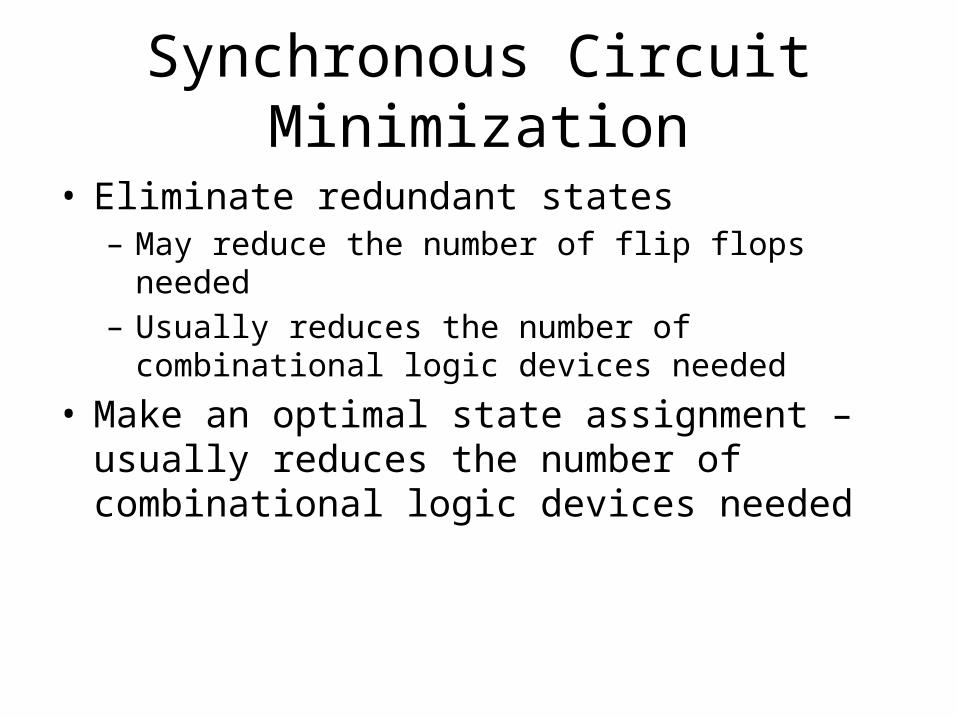
Synchronous Circuit Minimization

• Eliminate redundant states– May reduce the number of flip flops needed– Usually reduces the number of combinational logic devices

needed

• Make an optimal state assignment – usually reduces the number of combinational logic devices needed

Redundant States in Synchronous Circuits

Removal of redundant states is important because– Cost: the number of memory elements is directly related to the

number of states– Complexity: the more states the circuit contains, the more complex

the design and implementation becomes– Aids failure analysis: diagnostic routines are often predicated on the

assumption that no redundant states exist

Equivalent States

• States S1, S2, …, Sj of a completely specified sequential circuit are said to be equivalent if and only if, for every possible input sequence, the same output sequence is produced by the circuit regardless of whether S1, S2, …, Sj is the initial state.

• Let Si and Sj be states of a completely specified sequential circuit. Let Sk and Sl be the next states of Si and Sj, respectively for input Ip.

Si and Sj are equivalent if and only if for every possible Ip the following are conditions are satisfied.– The outputs produced by Si and Sj are the same,

– The next states Sk and Sl are equivalent.

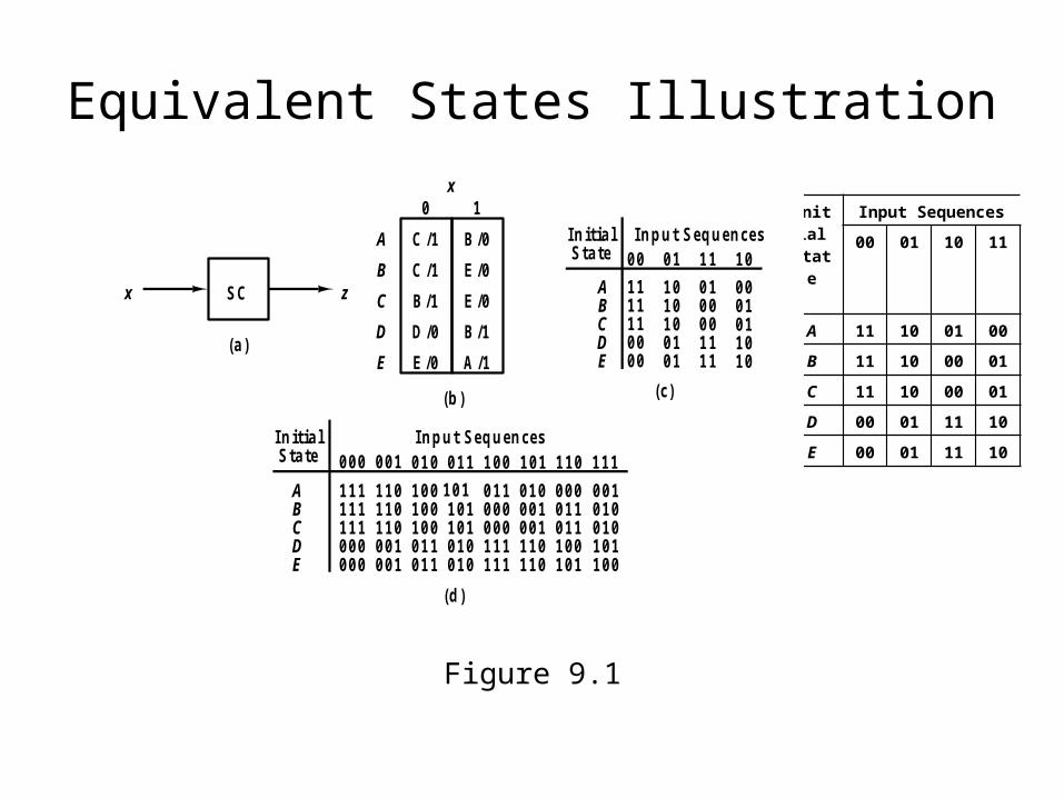
Equivalent States Illustration

S C

In itia lS ta te

zx

(d )

ABCDE

In p u t S eq u en ces0 0 0 0 0 1 0 1 0 0 11 1 0 0 1 0 1 11 0 11 1

11 111 111 10 0 00 0 0

11 011 011 00 0 10 0 1

1 0 01 0 01 0 00 110 11

1 0 11 0 11 0 10 1 00 1 0

0 110 0 00 0 011 111 1

0 1 00 0 10 0 111 011 0

0 0 00 110 111 0 01 0 1

0 0 10 1 00 1 01 0 11 0 0

(a )

(b )

0 1x

A

B

C

D

E

C /1

C /1

B /1

D /0

E /0

B /0

E /0

E /0

B /1

A /1

(c)

1111110 00 0

1 01 01 00 10 1

0 10 00 01111

0 00 10 11 01 0

ABCDE

In itia lS ta te

In p u t S eq u en ces0 0 0 1 1 011

Figure 9.1

InitialState

Input Sequences

00 01 10 11

A 11 10 01 00

B 11 10 00 01

C 11 10 00 01

D 00 01 11 10

E 00 01 11 10

Methods for Finding Equivalent States

• Inspection• Partitioning• Implication Tables

Finding Equivalent States By Inspection

0 1x

(a )

A

B

C

D

B /0

C /0

D /1

C /0

C /1

A /1

B /0

A /1

0 1x

(b )

A

B

C

B /0

C /0

B /1

C /1

A /1

B /0

0 1x

(c )

A

B

C

D

B /0

B /0

D /1

D /0

C /1

A /1

B /0

A /1

0 1x

(d )

A

B

C

B /0

B /0

B /1

C /1

A /1

B /0

0 1x

(e )

A

B

C

D

B /0D /0

D /1

B /0

C /1

A /1

B /0

A /1

Figure 9.2

Equivalence Relations

• Equivalence relation: let R be a relation on a set S. R is an equivalence relation on S if and only if it is reflexive, symmetric, and transitive. An equivalence relation on a set partitions the set into disjoint equivalence classes.

• Example: let S = {A,B,C,D,E,F,G,H} and R = {(A,A),(B,B),(B,H),(C,C),(D,D),(D,E),(E,E),(E,D),(F,F),(G,G),(H,H),(H,B)}. Then P = (A)(BH)(C)(DE)(F)(G)

• Theorem: state equivalence in a sequential circuit is an equivalence relation on the set of states.

• Theorem: the equivalence classes defined by the state equivalence of a sequential circuit can be used as the states in an equivalent circuit.

Finding Equivalent States by Partitioning

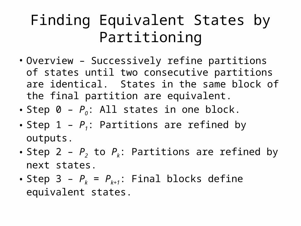
• Overview – Successively refine partitions of states until two consecutive partitions are identical. States in the same block of the final partition are equivalent.

• Step 0 – P0: All states in one block.

• Step 1 – P1: Partitions are refined by outputs.

• Step 2 – P2 to Pk: Partitions are refined by next states.

• Step 3 – Pk = Pk+1: Final blocks define equivalent states.

Partitioning Example

x0 1

A C/1 B/0B C/1 E/0C B/1 E/0D D/0 B/1E E/0 A/1

Reconsider the sequential circuit from Figure 9.1 (b)

P0 = (ABCDE)P1 = (ABC)(DE)P2 = (A)(BC)(D)(E)P3 = (A)(BC)(D)(E)

Hence, B ≡ C.

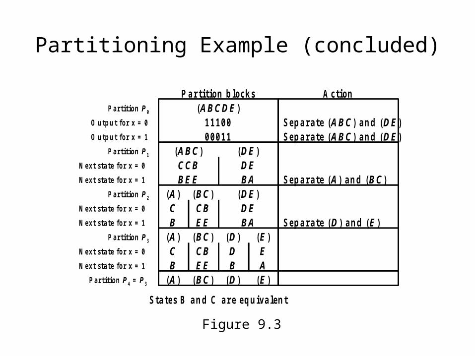
Partitioning Example (concluded)

P a rtit ion b locks A ctionP a rt it io n P 0

O u t p u t f o r x = 0

O u t p u t f o r x = 1

P a r t it io n P 1

N e x t s t a t e f o r x = 0

N e x t s t a t e f o r x = 1

P a r t it io n P 2

N e x t s t a t e f o r x = 0

N e x t s t a t e f o r x = 1

P a r t it io n P 3

N e x t s t a t e f o r x = 0

N e x t s t a t e f o r x = 1

P a r t it io n P 4 = P 3

(ABCDE )11 1 0 00 0 0 11

S ep a ra te (ABC ) a n d (DE )S ep a ra te (ABC ) a n d (DE )

(ABC )CCBBEE S ep a ra te (A ) a n d (BC )

S ep a ra te (D ) a n d (E )(BC )CBEE

(DE )DEBA

(A )CB

(BC )CBEE

(D )DB

(E )EA

S ta te s B a n d C a re eq u iva len t

(A )CB

(DE )DEBA

(BC )(A ) (D ) (E )

Figure 9.3

Test Your Understandingx

0 1A E/0 D/0B A/1 F/0C C/0 A/1D B/0 A/0E D/1 C/0F C/0 D/1G H/1 G/1H C/1 B/1

Find all equivalent states.

Test Your Understanding – Self Check

(a )

(b )

x0 1

E /0

A /1

C /0

B /0

D /1

C /0

H /1

C /1

D /0

F /0

A /1

A /0

C /0

D /1

G /1

B /1

A '

B '

C '

D '

E '

B '/0

A '/1

C '/0

E '/1

C '/1

A '/0

C '/0

A '/1

D '/1

B '/1

0 1xA

B

C

D

E

F

G

H

Figure 9.4

P0 = (ABCDEFGH)P1 = (AD)(BE)(CF)(GH)P2 = (AD)(BE)(CF)(G)(H)P3 = (AD)(BE)(CF)(G)(H)

A ≡ D: A’B ≡ E: B’C ≡ F: C’G: D’H: E’

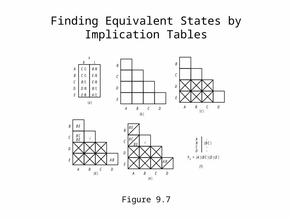
Finding Equivalent States by Implication Tables

Figure 9.7

(b )

B

C

D

E

B C DA

(a )

0 1x

A

B

C

D

E

C /1

C /1

B /1

D /0

E /0

B /0

E /0

E /0

B /1

A /1

(c)

B

C

D

E

B C DA

(d )

B

C

D

E

BE

BCBE

AB

B C DA

(e )

(f)

B

C

D

E

ABCD

BE

-(BC )

--

P K = (A )(BC )(D )(E )

BCBE

AB

B C DA

Example 9.6 -- An implication table example

(b )

B

C

D

E

ABCDEFG

(AF )(BC )(BH )(CH )----

N o te : (BC )(BH )(CH ) = (BCH )

BD

BC

B C DA

(a )

0 0 0 1x 1x 2

A

B

C

D

E

F

G

H

D /0

C /1

C /1

D /0

C /1

D /0

G /0

B /1

D /0

D /0

D /0

B /0

F /0

D /0

G /0

D /0

BD

AF

DF

DF

F GE

F

G

H

11 1 0

F /0

E /1

E /1

A /0

E /1

A /0

A /0

E /1

A /0

F /0

A /0

F /0

A /0

F /0

A /0

A /0

AF

DF

DG

AF

BG

AF

DG

AF

AFBC BC

(c )

P K = (AF )(BCH )(D )(E )(G )

AF