applications of statistical physics to problems in …coelhor/transfer_book.pdf · ·...
TRANSCRIPT

Applications of statistical physics toproblems in economics
Ricardo Coelho
Shool of Physics
Trinity College Dublin
Supervisor: Dr. Stefan Hutzler
Transfer Report April 2007


Abstract
Econophysics describes the application of tools from statistical physics to the study of problems
in economics such as correlations in stock prices or the distribution of wealth in society.
We present an analysis of financial data from stocks that belong to the London Stock Ex-
change, FTSE100, using the concept of random matrix theory and minimal spanning trees.
This reveals a division of the stocks in industrial sub-sectors, mostly in good agreement with
empirically derived groupings, but also indicating possible refinements, important for the use
in portfolio optimisation. A similar analysis of market indices of different countries shows that
despite globalisation strong regional geographical correlations still exist.
The general observation that the distribution of wealth in society takes the form of power-
laws is reproduced by various physical models, based on the analogy with collisions of particles
or Langevin type equations. We briefly review this and point to still existing difficulties in
explaining the details of the distribution.
Keywords: statistical physics, econophysics, random matrix theory, minimal spanning trees,
wealth distributions.
i

ii

Contents
Abstract i
1 Introduction 1
1.1 Stock Markets . . . . . . . . . . . . . . . . . . . . . . . . . . . . . . . . . . . . . . 1
1.2 Wealth Distributions . . . . . . . . . . . . . . . . . . . . . . . . . . . . . . . . . . 4
2 Methods 9
2.1 Analysing returns . . . . . . . . . . . . . . . . . . . . . . . . . . . . . . . . . . . . 9
2.2 The correlation of stock prices . . . . . . . . . . . . . . . . . . . . . . . . . . . . . 10
2.3 A Random Matrix Theory based analysis of stock correlations . . . . . . . . . . . 12
2.4 Minimal Spanning Trees . . . . . . . . . . . . . . . . . . . . . . . . . . . . . . . . 14
2.4.1 Distances . . . . . . . . . . . . . . . . . . . . . . . . . . . . . . . . . . . . 15
2.4.2 Mean Occupation Layer . . . . . . . . . . . . . . . . . . . . . . . . . . . . 17
2.4.3 Single and Multi Step Survival Rates . . . . . . . . . . . . . . . . . . . . . 17
3 Results 19
3.1 The correlations of stock prices . . . . . . . . . . . . . . . . . . . . . . . . . . . . 19
3.2 Random Matrix Theory . . . . . . . . . . . . . . . . . . . . . . . . . . . . . . . . 20
3.3 Minimal Spanning Trees . . . . . . . . . . . . . . . . . . . . . . . . . . . . . . . . 23
3.3.1 Distances . . . . . . . . . . . . . . . . . . . . . . . . . . . . . . . . . . . . 23
3.3.2 Mean Occupation Layer . . . . . . . . . . . . . . . . . . . . . . . . . . . . 26
3.3.3 Single and Multi Step Survival Rates . . . . . . . . . . . . . . . . . . . . . 26
4 Forward Plan 29
A Computation of parameters of T-student distribution 31
B Classification and legend for the industrial sectors of FTSE100 and the world
indices 33
iii

C List of Publications and Presentations 35
Bibliography 37
iv

Chapter 1
Introduction
“I think the next century will be the century of complexity.” (Stephen Hawking)
Econophysics describes the application of Physics concepts to the study of economics and
financial topics. This field had a big boom in the last decade when physicists started to look at
open problems in economics and with the large amount of financial data available started to see
many differences between the economic theory and empirical results.
Econophysics can be divided in two main areas:
• The first area and probably the main one, is related to the study of stock markets [1, 2].
• The second area is related to the study of wealth or income distributions in society. [3, 4].
The manipulation of Physics concepts in economics started more than 100 years ago when
Bachelier, in his doctoral thesis, Theorie de la speculation [5], was the first to formalise the
concept of random walks, predating the work of Einstein on Brownian motion.
1.1 Stock Markets
The area of study of stock markets has a big impact, because many physicist try to apply their
techniques to predict market oscillations or crashes, or to get better ways to filter data and
construct better portfolios of stocks, where the risk will be lower and the return higher.
An important issue is the huge amount of data that appeared from electronic formats. Nowa-
days it is possible to access 1 minute variations of prices of stocks in the market, which was
impossible some decades ago. In Figure 1.1 we can see an example of the daily evolution of the
price, Pi(t) of a company in time, in this case the bank HSBC (tick symbol HSBA) that belongs
to the main index of the London Stock Exchange, FTSE100. With the study of the distribution
of returns of the price of a stock, some empirical results didn’t match some laws used by the
1

2
economics community [6, 7, 8]. The returns are defined as: Ri(t) = ln Pi(t)− ln Pi(t−1) (Figure
1.2) and we use the logarithmic return for two reasons: first there is a common belief that the
price of stocks, Pi(t) increase exponentially, in time, on average; second is related with the fact
that the difference between two consecutive prices is very small, so:
Ri(t) = ln
(
Pi(t)
Pi(t − 1)
)
= ln
(
1 +Pi(t) − Pi(t − 1)
Pi(t − 1)
)
≈ Pi(t) − Pi(t − 1)
Pi(t − 1)(1.1)
i.e. the log-return has approximately the same value as the quotient return. The distribution of
returns generally does not follow a Gaussian, but as we can see from Figure 1.3 the tails of the
distribution are more enhanced than a Gaussian distribution. The strength of the tails depends
on the time scale at which returns are evaluated and scaling behaviour can be found for different
time scales [1]. Figures 1.2 and 1.3 are one example of the large study that we did for all the
stocks in our database.
10-1995 03-1997 07-1998 12-1999 04-2001 08-2002 01-2004 05-2005 10-2006
time (month - year)
250
500
750
1000
1250
Pric
e in
pou
nds
- P
( t )
Figure 1.1: Daily evolution of the price of the company HSBC (bank with the tick symbol
HSBA) in time.
An important issue is thus to redevelop financial tools that were developed from Gaussian
statistics, but now based on non-Gaussian statistics.
An important method frequently used for the study of time series in the stock market is
Random Matrix Theory. Random Matrix Theory was previously used in Nuclear Physics to
study the statistical behaviour of energy levels of nuclear reactions [9]. According to quantum
mechanics, the energy levels are given by the eigenvalues of a Hermitian operator, the Hamil-
tonian which was postulated to have independent random elements. However, analysis of the

1. Introduction 3
10-1995 03-1997 07-1998 12-1999 04-2001 08-2002 01-2004 05-2005 10-2006
time (month - year)
-0.1
-0.05
0
0.05
0.1
0.15
Ret
urn
- R
( t
)
Figure 1.2: Daily return of price of company HSBC (bank with the tick symbol HSBA) as a
function of time.
-0.2 -0.1 0 0.1 0.2R(t)
0.01
0.1
1
10
100
P (
R(t
) )
Figure 1.3: Normalised distribution of daily returns of price of company HSBC (bank with the
tick symbol HSBA) represented as black circles. The solid and broken lines represent fits to a
Gaussian and T-student distribution, respectively. The plot is in a log-linear scale. Note that
the data cannot be adequately represented by the Gaussian.

4
eigenvalues of real data showed deviations from the spectra of fully random matrices, thus in-
dicating non-random properties, useful for an understanding of the interactions between nuclei.
This approach is nowadays applied to the study of correlations of time series of returns in the
stock market (Section 2.2), where physicists try to find the non-random properties of the ma-
trix of correlations [10, 11, 12]. With the prediction of the eigensystem of a random matrix,
compared with the eigensystem of the matrix of real data of stocks, we can see eigenvalues far
from the prediction spectrum, that have a lot of information about the market [13, 14], as the
index of the market, or the clustering in industrial sector in markets. The index of the market
can be calculated as the simple mean of the prices of all the stocks that belong to the market
or the weighted mean, where some stocks contribute more to the index, related with the size of
the company. The industrial sectors can be different for different classifications, but normally
the industrial sector means which kind of business the company is included in.
To visualise the hierarchical structure of financial markets, Mantegna defined a distance
between stocks (Section 2.4.1), using the correlations between them [15]. Using this distance,
he constructed a network of stocks (Minimal Spanning Tree, Section 2.4), where nodes are
stocks and links are the distances between them. An example of a network of companies is
represented in Figure 1.4. The relations between companies show the formation of clusters of
sectors, as we can see that same symbols in Figure 1.4, are linked together. The 100 most highly
capitalised companies in the UK that comprise the London Stock Exchange FTSE100, represent
approximately 80% of the UK market. From these 100 stocks, we study the time series of the
daily closing price of 67 stocks that have been in the index continuously over a period of almost
9 years, starting in 2nd August 1996 until 27th June 2005. This equals 2322 trading days per
stock. The legend for the symbols and industrial sectors for the data of London Stock Exchange,
FTSE100 and for the World Indices data is explained in Appendix B. The tree represented in
Figure 1.4 is just one example of the many trees that we already produced in our work.
Properties of the trees, like topology for different time scales [16, 17], degree distribution of
the nodes [18, 19, 20, 21, 22], time evolution of moments of the distances of the trees [20, 21,
23, 24, 25, 26, 27], spread of nodes in the tree (Section 2.4.2) [20, 24, 25], robustness of the tree
(Section 2.4.3) [20, 21, 22, 24, 25, 26, 28], topology before and after financial crashes [26] and
others were studied for different kinds of data [29, 30].
1.2 Wealth Distributions
The area of study of wealth distributions is another important aspect of economics now looked
at by physicists, which is not only related with the study of wealth or income distributions in
societies [3], but also with the size of companies in a country [31], or the GDP (Gross Domestic

1. Introduction 5
III
ABF
ALLD
AZN
BAA
BA.
BARC
BATS
BG.
BOC
BOOT
BP.
BAY
BSY
BT.A
BNZL
CW.
CBRY
CPI
DMGT
DGE
DXNS
EMA
ETI
GSK
GUS
HNS
HAS
HSBA
JMAT
KGFLAND
LGENLII
LLOY
MKS
MRW
NGT
NXTOML
PSON
PRU
RB.
RTO
RTR
REX
RIORR.
RBSRSA
SGE
SBRY
SDR
SCTN
SPW
SVT
SHEL
SHP
SN.
STAN
TATETSCO
ULVR
VOD
WTB
WOS
WPP
Pajek
Figure 1.4: MST of 67 stocks of the main index of the London Stock Exchange (FTSE100)
computed from the time series of returns for each stock. For this tree we use the full time series
of 2322 daily prices from 2nd August 1996 until 27th June 2005. A division in clusters can be
seen from the figure where one sector (grey ◦) is the backbone of the tree and many sectors are
linked with this one. The classification of the sectors is presented in Appendix B.
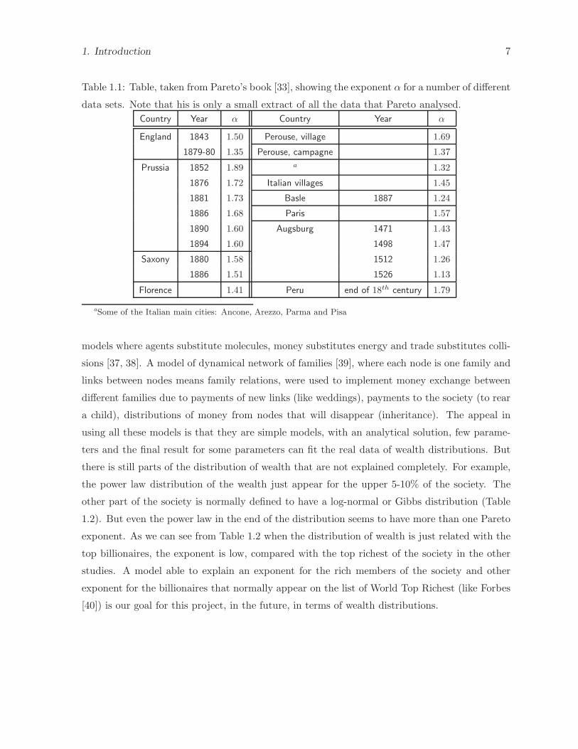
Product) of countries [32]. The study of wealth distributions has attracted great interest since
the work of the socio-economist Vilfredo Pareto, who wrote a book about economical politics,
100 years ago [33], studying a large amount of economical data (Table 1.1), he suggested that
the distribution of wealth from different cities and countries follow a power law distribution with
similar exponents α (between 1 and 2), known nowadays as Pareto’s index:
P (w) ∼ w−(1+α), for large w. (1.2)
The power law distribution is also known as Pareto’s Law and sketches of both probability
distribution and cumulative distribution are shown in Figures 1.5 and 1.6, respectively. The
cumulative distribution of wealth is known as the probability that the wealth takes on a value
equal of bigger than w:
C(>w) ∼ w−α, for large w. (1.3)
This work of Pareto was the first empirical study of wealth distributions, but over the last
decade many physicists studied an extensive amount of data from different countries, summarised
in Table 1.2.

6
P (w)
w
Figure 1.5: Sketch of the distribution of income according to Pareto. For large values of income
this follows a power law.
log w
log C(>w)
Figure 1.6: Sketch of the cumulative distribution of income. In this log− log plot the power-law
regime results in a straight line with slope −α.
Apart from the study of the empirical data, physicist are very interested in modelling wealth
distributions [34]. A detailed review of some models and open problems in the study of wealth
distribution [35] was published by us in a chapter of an Econophysics book [4]. Models used in
biological systems like Lotka-Volterra models, were used by physicists to explain the economic
trade relations in communities [36]. Gas models of collisions were transformed into economic
1. Introduction 7
Table 1.1: Table, taken from Pareto’s book [33], showing the exponent α for a number of different
data sets. Note that his is only a small extract of all the data that Pareto analysed.
Country Year α Country Year α
England 1843 1.50 Perouse, village 1.69
1879-80 1.35 Perouse, campagne 1.37
Prussia 1852 1.89 a 1.32
1876 1.72 Italian villages 1.45
1881 1.73 Basle 1887 1.24
1886 1.68 Paris 1.57
1890 1.60 Augsburg 1471 1.43
1894 1.60 1498 1.47
Saxony 1880 1.58 1512 1.26
1886 1.51 1526 1.13
Florence 1.41 Peru end of 18th century 1.79
aSome of the Italian main cities: Ancone, Arezzo, Parma and Pisa
models where agents substitute molecules, money substitutes energy and trade substitutes colli-
sions [37, 38]. A model of dynamical network of families [39], where each node is one family and
links between nodes means family relations, were used to implement money exchange between
different families due to payments of new links (like weddings), payments to the society (to rear
a child), distributions of money from nodes that will disappear (inheritance). The appeal in
using all these models is that they are simple models, with an analytical solution, few parame-
ters and the final result for some parameters can fit the real data of wealth distributions. But
there is still parts of the distribution of wealth that are not explained completely. For example,
the power law distribution of the wealth just appear for the upper 5-10% of the society. The
other part of the society is normally defined to have a log-normal or Gibbs distribution (Table
1.2). But even the power law in the end of the distribution seems to have more than one Pareto
exponent. As we can see from Table 1.2 when the distribution of wealth is just related with the
top billionaires, the exponent is low, compared with the top richest of the society in the other
studies. A model able to explain an exponent for the rich members of the society and other
exponent for the billionaires that normally appear on the list of World Top Richest (like Forbes
[40]) is our goal for this project, in the future, in terms of wealth distributions.

8
Table 1.2: Table of empirical data. In column Source: S.H. - Size of Houses; I. - Income; I.T. -
Income Tax; Inhe. T. - Inheritance Tax; W. - Wealth. In column Distributions: Par. - Pareto
tail; LN - Log-normal; Exp. - Exponential; D. Par. - Double Pareto Log-normal; G. - Gamma.Country Source Distributions Pareto Exponents Ref.
Egypt S.H. (14thB.C.)a Par. α = 1.59 ± 0.19 [41]
Japan I.T. (1992) Par. α = 2.057 ± 0.005 [42, 43, 44]
I. (1998) Par. α = 1.98
I.T. (1998) Par. α = 2.05
I. / I.T. (1998) Par. α = 2.06
I. (1887-2000) LN / Par. α ∼ 2.0b
U.S.A. I.T. (1997) Par. α = 1.6 [45]
Japan I.T. (2000) Par. α = 2.0
U.S.A. I. (1998) Exp. / Par. α = 1.7 ± 0.1 [46, 47, 48]
U.K. Inhe. T. (1996) Exp. / Par. α = 1.9
Italy I. (1977-2002) LN / Par. α ∼ 2.09 − 3.45 [49]
I. (1987) LN / Par. α = 2.09 ± 0.002
I. (1993) LN / Par. α = 2.74 ± 0.002
I. (1998) LN / Par. α = 2.76 ± 0.002
Australia I. (1993-97) Par. α ∼ 2.2 − 2.6 [50]
U.S.A. I. (1997) D. Par.c α = 22.43 / β = 1.43 [51]
Canada I. (1996) D. Par. α = 4.16 / β = 0.79
Sri-Lanka I. (1981) D. Par. α = 2.09 / β = 3.09
Bohemia I. (1933) D. Par. α = 2.15 / β = 8.40
U.S.A. 1980 G. / Par. α = 2.2 [52]
1989 G. / Par. α = 1.63
2001 G. / Par.
U.K. 1996 Par. α = 1.85
1998-99 Par. α = 1.85
U.S.A. I. (1992) Exp. / LN d [53]
U.K. I. (1992-2002) Exp. / LN
India W. (2002-2004)e Par. α ∼ 0.81 − 0.92 [54]
I. (1997) Par. α = 1.51
U.S.A. W. (1996)f Par. α = 1.36 [55, 56, 57]
W. (1997)g Par. α = 1.35
U.K. W. (1970) Par.
W. (1997)h Par. α = 1.06
Sweden W. (1965) Par. α = 1.66
France W. (1994) Par. α = 1.83
U.K. Inhe. T. (2001) Par. α = 1.78 [39]
Portugal I.T. (1998-2000) Par. α ∼ 2.30 − 2.46 [58]
aRelated to the size of houses found in an archaeological study.bThis value is an average Pareto exponent.cα and β are Pareto exponents for the richest and poorest part, respectively.dBoth distributions are a good fit of the data.e125 wealthiest individuals in India.f400 wealthiest people, by Forbes.gTop wealthiest people, by Forbes.hTop wealthiest people, by Sunday Times.
Chapter 2
Methods
The computational part of our work concerns the analysis of financial data. Nowadays, we can
find much financial data on the Internet [59], but there is a big problem with this: parts of
data are missing, so in the beginning of our work, before uploading the data to a database, we
have to check what we can use and what we cannot. Which days are missing, which stocks are
missing, even the format of the data that we download from the Internet needs to be converted
in a different format for our database.
We create a MySQL database [60], where we upload all our data. After uploading the data
we have to classify the data, for example, if we have data from stocks of the London Stock
Exchange, and we just have the tick symbol of each company we will need to check the sector
or industry to which one belongs. But there is more than one classification, so we have to
test different classifications and see which one is more powerful for our study. With the term
powerful we mean the classification that will show the better visualisation of clusters of sectors
in the Minimal Spanning Tree, for example.
In this chapter, we will discuss the methods used until now.
2.1 Analysing returns
As we already said in the Introduction, some economists assume the returns to be Gaussian
distributed, but we saw in Figure 1.3 that the tails of the distribution are “fatter” than a
Gaussian distribution. To fit the Gaussian distribution we computed the mean (µ) and standard
deviation (σ) of the returns and plotted the probability distribution function:
P (x) =1
σ√
2πexp
(
−(x − µ)2
2σ2
)
(2.1)
But we can fit distributions with fat tails, like the T-student or Tsallis distribution [61]
to the distribution of returns and see if the tails are better fitted with this. The probability
9

10
distribution function of a T-student is given as:
Pk(x) = Nk1
√
2πσ2k
e−x2/2σ2
k
k (2.2)
where Nk is a normalisation factor:
Nk =Γ(k)√
kΓ(
k − 12
) (2.3)
and Γ(k) = (k− 1)! is the Gamma function. The factor σk = σ√
(k − 3/2)/k is related with the
effective standard deviation of the distribution (σ) and with the degree of distribution (k). The
function ezk is an approximation of the exponential function called k-exponential:
ezk = (1 − z/k)−k (2.4)
and in the limit k → ∞ this function reduces to the ordinary exponential function. The proba-
bility distribution function can be written as:
Pk(x) =Γ(k)
Γ(
k − 12
)
1
σ√
π(2k − 3)
[
1 +x2
σ2(2k − 3)
]−k
(2.5)
The parameter k is related with the Tsallis parameter q by k = 1/(q − 1). The computation
of the parameters of T-student distribution is explained in Appendix A. For all the stocks of
the London Stock Exchange that we studied, the minimum value of k is 1.7 and the maximum
9.0, but most of the values are in the [2, 4] interval, which means values of q in the [1.25, 1.5]
interval, that is around the values found by Tsallis [62] (1.40, 1.37 and 1.38) for 1−, 2− and 3−minutes return, respectively, for the NYSE in 2001. For example the value of k found for HSBC
company is ∼ 2.90 (the one used in the T-student distribution in Figure 1.3).
Our study is based on the assumption that the returns of the stock price carry more informa-
tion than random noise. To check this, we will compute the correlation between returns of stock
prices and analyse the correlation matrix. The main idea of our work is to find the underlying
correlation matrix of stock returns.
2.2 The correlation of stock prices
The correlation coefficient, ρij between stocks i and j is given by:
ρij =〈RiRj〉 − 〈Ri〉〈Rj〉
√
(
〈R2i 〉 − 〈Ri〉2
)
(
〈R2j 〉 − 〈Rj〉2
)
(2.6)
where Ri is the vector of the time series of log-returns, Ri(t) = ln Pi(t) − ln Pi(t − 1) and Pi(t)
is the daily closure price of stock i at day t. The notation 〈· · ·〉 means an average over time

2. Methods 11
1T
∑t+T−1t′=t · · ·, where t is the first day and T is the length of our time series. We can normalise
the time series of returns for each stock by subtracting the mean and dividing by the standard
deviation:
Ri =Ri− < Ri >
√
〈R2i 〉 − 〈Ri〉2
(2.7)
The correlation coefficient is then given by: ρij = 〈RiRj〉.This coefficient can vary between −1 ≤ ρij ≤ 1, where −1 means completely anti-correlated
stocks and +1 completely correlated stocks. If ρij = 0 the stocks i and j are uncorrelated.
The coefficients form a symmetric N × N matrix with diagonal elements equal to unity. The
correlation matrix with elements ρij can be represented as:
C =1
TGGT (2.8)
where G is an N × T matrix with elements Ri(t) and GT denotes the transpose of G.
The distribution of correlation coefficients is an important aspect of our study because can
show how the stocks from a portfolio are related with each other. If we compare the distribution
of real data with the one made from random data (Figure 3.1), conclusions about the non-
randomness of the market can be done. We can also study the moments of this distribution, as
the mean [20, 25]:
ρ =2
N(N − 1)
∑
i<j
ρij (2.9)
the variance:
λ2 =2
N(N − 1)
∑
i<j
(ρij − ρ)2, (2.10)
the skewness:
λ3 =2
N(N − 1)λ3/22
∑
i<j
(ρij − ρ)3, (2.11)
and the kurtosis:
λ4 =2
N(N − 1)λ22
∑
i<j
(ρij − ρ)4. (2.12)
Just the elements of the upper triangle of the matrix are used to compute the matrix, because
it’s a symmetric matrix with diagonal elements equal to unity. If we divide our time series
in small windows and we move these windows in small steps, we create different correlation
matrices, and if we compute the moments of each matrix, we can study these moments in time.

12
2.3 A Random Matrix Theory based analysis of stock correla-
tions
Studying the eigensystem of the correlation matrix, we can see some financial information in
the eigenvalues of the matrix and in the respective eigenvectors. We know that comparing the
spectrum of eigenvalues of correlation matrix with the spectrum of eigenvalues of a random
matrix, we can extract information about the market and about the sectors that constitute the
market. A random matrix is defined by [63]:
C′ =1
TG′G′T (2.13)
where G′ is a N × T matrix with columns of time series with zero mean and unit variance, that
are uncorrelated, the spectrum of eigenvalues can be calculated analytically. In the limit N → ∞and T → ∞, where Q = T/N is fixed and bigger than 1, the probability density function of
eigenvalues of the random matrix is:
PRM (λ) =Q
2π
√
(λmax − λ)(λ − λmin)
λ(2.14)
where
λmaxmin =
(
1 ± 1√Q
)2
(2.15)
limits the interval where the probability density function is different from zero. The PRM (λ)
for Q = 34.6 (T = 2321 and N = 67 are the values for our London Stock Exchange data) is
shown in Figure 2.1 and it’s compared with the distribution of eigenvalues of a correlation matrix
computed from shuffled time series of original data of stocks from the London Stock Exchange.
If we compare the results of a correlation matrix constructed with real time series, with
the random matrix (Figure 3.3) we can see that the highest eigenvalues of the real matrix are
much higher than the highest eigenvalue of random matrix. The largest eigenvalue represents
something that is common to all stocks. If we analyse the respective eigenvector, all the stocks
have the same sign (Figure 3.4), so all participate in the same way.
The largest eigenvalue and its corresponding eigenvector can be interpreted as the collective
response of the market to any external factors, so it can be compared with the market index
[13, 14]. A way to prove this is to see the correlation between the index of the market and the
projection of the time series in the eigenvector related with the largest eigenvalue (Figure 3.5).
The projection is given by:
RN (t) =
N∑
i=1
uNi Ri(t) (2.16)
where RN (t) is the return of the portfolio of N stocks, defined by the eigenvector uN and we
call it market mode.

2. Methods 13
0.6 0.8 1 1.2 1.4 1.6 1.8 2
Eigenvalue λ0
0.5
1
1.5
2
2.5
3
P RM
( λ
)
Figure 2.1: Spectrum of the eigenvalues of random correlation matrix, computed using 2.14
with Q = 34.6, in bold compared with the normalised distribution of eigenvalues of a correlation
matrix computed from shuffled time series, that should be similar to random time series but
with the same distribution as the original time series of returns.
If we filter the real time series, extracting the market mode from every stock, we get a new
correlation matrix with the residuals Cres [14]. A way to filter the market mode is to use the
one-factor model or Capital Asset Pricing model [64], where the return of the price can be
expressed as:
Ri(t) = αi + βiRN (t) + ǫi(t) (2.17)
The first term is the mean of the returns, the second term is the influence of the market index
and the last term is the residual. If we fit every time series (Ri(t) for every i) to the time series
of market mode (RN (t)) using the least square regression, we can get the values of parameters
α and β:
αi = < Ri > −βi < RN >
βi =cov(Ri, R
N )
σ2RN
(2.18)
where σRN is the standard deviation of the market mode and cov() is the covariance.
The residuals are given by:
ǫi(t) = Ri(t) − αi − βiRN (t) (2.19)
and we can compute the matrix of residuals with these new time series.
14
If we analyse the spectrum of eigenvalues of the new filtered matrix, some eigenvalues con-
tinue to be far outside the range obtained from equation 2.14 . These are the eigenvalues that
represent different sectors. Our main work is to try to understand a way to filter this informa-
tion, to end up with a time series of random information. Our approach is to use a multifactor
model, where we not just use a market mode, but also a sector mode [65, 66]. This sector
mode is defined for each sector in our portfolio and is related with the highest eigenvalue of the
correlation matrix of the stocks of only one sector, similar to what we did for the whole market.
Our multifactor model can be represented as:
Ri(t) = αi + βiRN (t) +
NS∑
j=1
γijRSj(t) + ǫi(t) (2.20)
where j represent the index of the sector presented in the portfolio. The new term has the
sector mode RSj (t) and a parameter γij that is only different from zero if the stock belongs to
the sector j. As we did before, we can now filter our time series by subtracting the market and
sector modes:
ǫi(t) = Ri(t) − αi − βiRN (t) −
NS∑
j=1
γijRSj(t) (2.21)
We use least square fitting to find the values of the parameters:
αi = < Ri > −βi < RN > −γij < RSj >
βi =cov(Ri, R
N ) − γijcov(RSj , RN )
σ2RN
γi =cov(Ri, R
Sj )σ2RN − cov(Ri, R
N )cov(RSj , RN )
σ2RSj
σ2RN −
[
cov(RSj , RN )]2 (2.22)
We will need to check if this model is enough to represent the returns of the stocks, or if
there are other terms, like for example a term of correlations between stocks of different sectors.
2.4 Minimal Spanning Trees
Another way to study the correlation of stocks is to create a matrix of distances between stocks
from the correlation coefficients. With this matrix of distances we can create a tree where
nodes are stocks and links are the distance between the stocks. If two stocks are correlated, the
distance between them is small. The tree that we use to study these properties is the Minimal
Spanning Tree (MST).

2. Methods 15
2.4.1 Distances
The metric distance, introduced by Mantegna [15], is determined from the Euclidean distance
between vectors, dij = |Ri − Rj |. Because |Ri| = 1 it follows that:
d2ij = |Ri − Rj |2 = |Ri|2 + |Rj |2 − 2Ri · Rj = 2 − 2ρij (2.23)
This relates the distance of two stocks to their correlation coefficient:
dij =√
2(1 − ρij) (2.24)
This distance varies between 0 ≤ dij ≤ 2 where small values imply strong correlations between
stocks. Following the procedure of Mantegna [15], this distance matrix is now used to construct
a network with the essential information of the market.
This network (MST) has N − 1 links connecting N nodes. The nodes represent stocks and
the links are chosen such that the sum of all distances (normalised tree length) is minimal. We
perform this computation using Prim’s algorithm [67]. The Prim’s algorithm is given by:
• Choose the minimum distance between a pair of stocks and construct a link between them;
• Choose the next minimum distance between a pair of stocks, where one of the stocks
already has a link but the other does not have any links. If the conditions are respected
construct a link between them, if not, choose the next minimum distance where this is
obeyed;
• Continue to choose pairs of stocks to link, with the conditions to verify until we reach
N − 1 links.
With the information of which stocks are connected to one another, we use the Pajek software
to visualise these links [68]. The Pajek software uses the Kamada-Kawai algorithm [69] to display
the links and nodes. This algorithm introduce a dynamic system in which every two nodes are
connected by a “spring” with the respective distance between two stocks. The optimal layout of
vertices is when the total spring energy is minimal. As we saw in Figure 1.4 of the Introduction,
a MST of stock data is almost organised in clusters of different industrial sectors of the market.
The main idea for using MST, apart of the visualisation of links between companies, is to
filter data. From the N × (N − 1)/2 correlation coefficients we are only left with N − 1 points,
which we believe are the most important coefficients of the correlation matrix.
To see better this clustering property we developed a new kind of tree, where the stocks, if
they belong to the same sector and are linked together, emerge in one big node. The sizes of
the final nodes are proportional to the number of stocks that they contain, as shown in Figure
2.2.

16
Pajek
Figure 2.2: New visualisation of the clusters of the MST of figure 1.4. The meaning of the
symbols is explained in Appendix B.
As we did for the correlations, we study the distribution of distances in the tree and the
main moments, as the mean or normalised tree length:
L =1
N − 1
∑
dij∈Θ
dij (2.25)
where Θ represents the MST. The other moments are the variance:
ν2 =1
N − 1
∑
dij∈Θ
(dij − L)2, (2.26)
the skewness:
ν3 =1
(N − 1)ν3/22
∑
dij∈Θ
(dij − L)3, (2.27)
and the kurtosis:
ν4 =1
(N − 1)ν22
∑
dij∈Θ
(dij − L)4. (2.28)
Again we can divide our time series in small windows and move those windows in small steps,
creating different MST. If we compute the moments of each MST, we can study these moments
in time.

2. Methods 17
2.4.2 Mean Occupation Layer
Changes in the density, or spread, of the MST can be examined through calculation of the mean
occupation layer, as defined by Onnela et al. [20]:
l(t, vc) =1
N
N∑
i=1
L(vti), (2.29)
where L(vti) denotes the level of a node, or vertex, vt
i in relation to the central node, whose level
is defined as zero. The central node can be defined as the node with the highest number of links
or as the node with the highest sum of correlations of its links. Both criteria produce similar
results. The mean occupation layer can then be calculated using either a fixed central node for
all windows, or with a continuously updated node.
2.4.3 Single and Multi Step Survival Rates
Finally, the robustness of links over time can be examined by calculating survival ratios of links,
or edges in successive MST. The single-step survival ratio is the fraction of links found in two
consecutive MST in common at times t and t − 1 and is defined by Onnela et al. [20] as:
σ(t) =1
N − 1|E(t) ∩ E(t − 1)| (2.30)
where E(t) is the set of edges of the MST at time t, ∩ is the intersection operator, and | · · · |gives the number of elements in the set. A multi-step survival ratio can be used to study the
longer-term evolution [20]:
σ(t, k) =1
N − 1|E(t) ∩ E(t − 1) · · ·E(t − k + 1) ∩ E(t − k)| (2.31)
in which only the connections that continue for the entire period without any interruption are
counted.

18

Chapter 3
Results
The data that we have in our database is daily prices from stocks of the main index of the
London Stock Exchange, FTSE100; weekly price from indices all around the world; daily price
from stocks of the main index in Euronext Lisbon, PSI20; daily prices of more than 6000 stocks
all over the world; Forbes’ list of top richest individuals in World from 1996 to 2006. In this
section, the results presented are from the daily prices of stocks of the London Stock Exchange,
FTSE100 and from weekly price of world indices.
3.1 The correlations of stock prices
The distribution of coefficients of the correlation matrix constructed from the time series of
stocks of the FTSE100, is shown in Figure 3.1 and compared with the distribution of coefficients
of a correlation matrix of shuffled time series. The results of the shuffle time series are similar
with the one for random time series, because the correlation in time of different companies is
destroyed. As expected for a random matrix, the distribution of the coefficients for the shuffle
time series is symmetric and with zero mean, different from the original time series, where the
distribution is asymmetric with non-zero mean. But the distribution depends on the length T
of the time series and depends on external aspects that affect the market as we can see in Figure
3.2. If we divide our time series in small windows and we move these windows in time, we will
get different matrices of correlations and different distributions of the coefficients. We do this in
order to see the market changes. We choose to divide the time series in windows of size 500 days
and move them day by day, so we will get 1822 (2322−500) different matrices. In Figure 3.2 we
can see the moments of the distribution of coefficients in time where the mean and variance are
highly correlated (0.779), the skewness and kurtosis are also highly correlated and the mean and
skewness are anti-correlated. This implies that when the mean correlation increases, usually
after some negative event in market, the variance increases. Thus the dispersion of values
19

20
of the correlation coefficient is higher. The skewness is almost always positive, which means
that the distribution is asymmetric, but after a negative event the skewness decreases, and the
distribution of the correlation coefficients becomes more symmetric.
0 0.2 0.4 0.6 0.8ρ
ij
0
5
10
15
20
P (
ρ ij )
Figure 3.1: Distribution of coefficients of correlations between 67 stocks of the FTSE100, the
main index of the London Stock Exchange. The time series of each stock have 2322 days,
resulting in 2321 returns. The solid line represents the distribution for the original time series
and the broken line represents the distribution for the time series after been shuffled. The
shuffled time series work like random time series but with the same distribution of returns as
the original one.
3.2 Random Matrix Theory
Comparing the probability density functions of eigenvalues of random matrix, PRM (λ) with the
real correlation matrix, Preal(λ) we can see that some eigenvalues are way out of the spectrum
of the random matrix (Figure 3.3). We can regard this as the information of the market that is
not random. All the eigenvalues that are outside the region defined by random matrix theory
contain information that can be revealed when we look closer at the respective eigenvectors.
The elements of the eigenvector related with the largest eigenvalue are represented in Figure 3.4
and as we can see, they all have the same sign. Comparing the market mode constructed from
this eigenvector (equation 2.16) with the real index of the FTSE100, we can see a very high
correlation of 0.95 (Figure 3.5).

3. Results 21
0
0.1
0.2
0.3
0.4
mea
n0.008
0.010.0120.0140.0160.0180.02
vari
ance
-0.4-0.2
00.20.40.60.8
1
skew
ness
02-1996 11-1996 09-1997 07-1998 05-1999 03-2000 01-2001 11-2001 08-2002 06-2003time (month - year)
33.5
44.5
55.5
6
kurt
osis
Figure 3.2: Mean (eq. 2.9), variance (eq. 2.10), skewness (eq. 2.11) and kurtosis (eq. 2.12) of the
correlation coefficients of the matrix constructed from time series of 67 stocks of the FTSE100.
We use time windows of length T = 500 days and window step length parameter δT = 1 day.
0 5 10 15
Eigenvalue λ0
0.5
1
1.5
2
P real
( λ
)
Figure 3.3: Empirical spectrum of the eigenvalues of correlation matrix constructed from time
series of 67 stocks of the FTSE100, compared with the analytical spectrum of the random matrix,
equation 2.14 (bold curve).

22
JM
AT
BO
C
RIO
TA
TE
BA
TS
RB
.
ALLD
SC
TN
AB
F
CB
RY
DG
E
UL
VR
ET
I
MR
W
BO
OT
WT
B
DX
NS
TS
CO
NX
T
EM
A
SB
RY
MK
S
GU
S
BS
Y
DM
GT
KG
F
PS
ON
RT
R
WP
P
BA
Y LII
LA
ND
OM
L
SD
R
ST
AN
RS
A III
RB
S
LG
EN
HS
BA
BA
RC
LLO
Y
PR
U
SH
P
SN
.
AZ
N
GS
K
HN
S
RE
X
BA
.
BN
ZL
RT
O
CP
I
WO
S
HA
S
BA
A
RR
.
BG
.
BP
.
SH
EL
SG
E
CW
.
BT
.A
VO
D
SV
T
SP
W
NG
T
0.000
0.050
0.100
0.150
0.200
Basic_materials
Consumer_goods
Consumer_services
Financials
Health_care
Industrials
Oil_and_gas
Technology
Telecommunications
Utilities
Figure 3.4: Elements of the highest eigenvector of the real correlation matrix constructed from
time series of 67 stocks of the FTSE100.
-6 -4 -2 0 2 4 6
Normalized Index FTSE100 - RM
(t)
-6
-4
-2
0
2
4
6
Nor
mal
ized
Ind
ex -
R67
(t)
0.95
Figure 3.5: Returns of the portfolio of 67 stocks of FTSE100 using the definition of equation
2.16 against the real index of FTSE100 in time. The correlation between them is high, 0.95.
Analysing the eigensystem of the residual matrix (Cres) we conclude that the eigenvector of
the highest eigenvalue (Figure 3.6) is the same as the second eigenvector of the original matrix.

3. Results 23
So, we conclude that we are able to filter the influence of the market from our time series. This
eigenvector has information about the sectors. Stocks from the same sector that have different
signs are not clustered together when we see them in the MST (Figure 1.4), but if they have the
same sign they form a cluster. We can see that these companies belong to different sub-sectors
(Appendix B).
JM
AT
RIO
BO
C
TA
TE
BA
TS
AB
F
AL
LD
RB
.
SC
TN
CB
RY
UL
VR
DG
E
RT
R
WP
P
PS
ON
BS
Y
EM
A
DM
GT
DX
NS
BA
Y
ET
I
GU
S
NX
T
MK
S
KG
F
MR
W
WT
B
BO
OT
TS
CO
SB
RY III
OM
L
HS
BA
SD
R
ST
AN LII
RS
A
PR
U
RB
S
BA
RC
LA
ND
LG
EN
LLO
Y
SH
P
SN
.
AZ
N
GS
K
CP
I
HA
S
RR
.
HN
S
WO
S
BN
ZL
RE
X
BA
.
RT
O
BA
A
BG
.
BP
.
SH
EL
SG
E
CW
.
VO
D
BT
.A
NG
T
SP
W
SV
T
-0.300
-0.200
-0.100
0.000
0.100
0.200
0.300
Basic_materials
Consumer_goods
Consumer_services
Financials
Health_care
Industrials
Oil_and_gas
Technology
Telecommunica-tions
Utilities
Figure 3.6: Elements of the highest eigenvector of the correlation matrix of residuals (Cres)
constructed from filtered time series of 67 stocks of the FTSE100.
The correlation between the sector mode and the real index, FTSE100 is different for different
sectors. For example, Financial has a large correlation of 0.882, but Health Care have a negative
correlation of −0.673, as we can see in Figures 3.7 and 3.8.
3.3 Minimal Spanning Trees
3.3.1 Distances
To see how the results of the MST are similar with the results from the correlation matrix, we
compute the moments of the distances of the tree in time and compare with the same moments
for the correlation coefficient (Figure 3.9). As expected from equation 2.24, when the mean
correlation increases, the mean distance decreases and vice versa. Here, the mean and the
variance of the distances of the tree are anti-correlated but the skewness and the mean continue
to be anti-correlated. This means that after some negative event impacts the market, the tree
shrinks, so the mean distance decreases [26], the variance increases implying a higher dispersion

24
-6 -4 -2 0 2 4 6
Normalized Index FTSE100 - RM
(t)
-6
-4
-2
0
2
4
6
Nor
mal
ized
Ind
ex o
f Fi
nanc
ial S
ecto
r
0.882
Figure 3.7: Returns of the portfolio of the stocks of FTSE100 that belong to Financial Sector
using the definition of equation 2.16 against the real index of FTSE100 in time. The correlation
between them is high, 0.882.
-6 -4 -2 0 2 4 6
Normalized Index FTSE100 - RM
(t)
-6
-4
-2
0
2
4
6
Nor
mal
ized
Ind
ex o
f H
ealth
Car
e Se
ctor
-0.673
Figure 3.8: Returns of the portfolio of the stocks of FTSE100 that belong to Health Care Sector
using the definition of equation 2.16 against the real index of FTSE100 in time. They are
anticorrelated with a value of −0.673.

3. Results 25
of the values of distance and the skewness, that is almost always negative, increases showing
that the distribution of the distances of the MST gets more symmetric.
0.951
1.051.1
1.151.2
mea
n
0.0080.01
0.0120.0140.0160.0180.02
vari
ance
-2
-1.5
-1
-0.5
0
skew
ness
02-1996 11-1996 09-1997 07-1998 05-1999 03-2000 01-2001 11-2001 08-2002 06-2003time (month - year)
2
3
4
5
6
7
kurt
osis
Figure 3.9: Mean (eq. 2.25), variance (eq. 2.26), skewness (eq. 2.27) and kurtosis (eq. 2.28)
of the distances of the MST constructed from time series of 67 stocks of the FTSE100. We use
time windows of length T = 500 days and window step length parameter δT = 1 day.
A MST visualisation for our study of the world indices is shown in Figure 3.10. The clusters
which we observe appear to be organized principally according to a geographical criterion. With
the highest number of links, France can be considered the central node. Closely connected to
France are a number of the more developed European countries. We can also identify several
branches which form the major subsets of the MST and these can then be broken down into clus-
ters. The Netherlands heads a branch that includes clusters of additional European countries.
The U.S.A. links a cluster of North and South American countries to France via Germany. Aus-
tralia heads a branch with several groupings: all the Asian-Pacific countries form two clusters,
one of more developed and the other of less advanced countries. Most of the Central and East
European (CEE) countries, that joined the E.U. in 2004, form a cluster. Jordan, which appears
in a European clustering, is an apparent anomaly. This is likely due to the fact that Jordan is
the last node connected to the network and has correlations with other countries close to zero,
which means a relatively high minimum distance. We can conclude that Jordan is an outlier of
our study that does not have any close relation to any of the other countries represented here.

26
ARG
AUS
AUT
BEL
BRZCAN
CHFCHLCOL
CRTCZK
DNK
ESP
FINFRAGER
GRC
HK
HUN
ICE
IDO
IND
IRE ISR
ITA
JAP
JOR
LTU
MAL
MEX
MTA
NEZ
NLDNOR
PAK
PER
PHI
POL
PRT
ROMRUS SAF
SGP
SOK
SVK
SVN
SWE
THI
TUK
TWA
UK
USA
VEZ
Pajek
Figure 3.10: MST of 53 countries computed from the time series of returns for each country
market index. For this tree we use the full time series of 475 weekly prices from 8th January
1997 until 1st February 2006. The classification is presented in Appendix B.
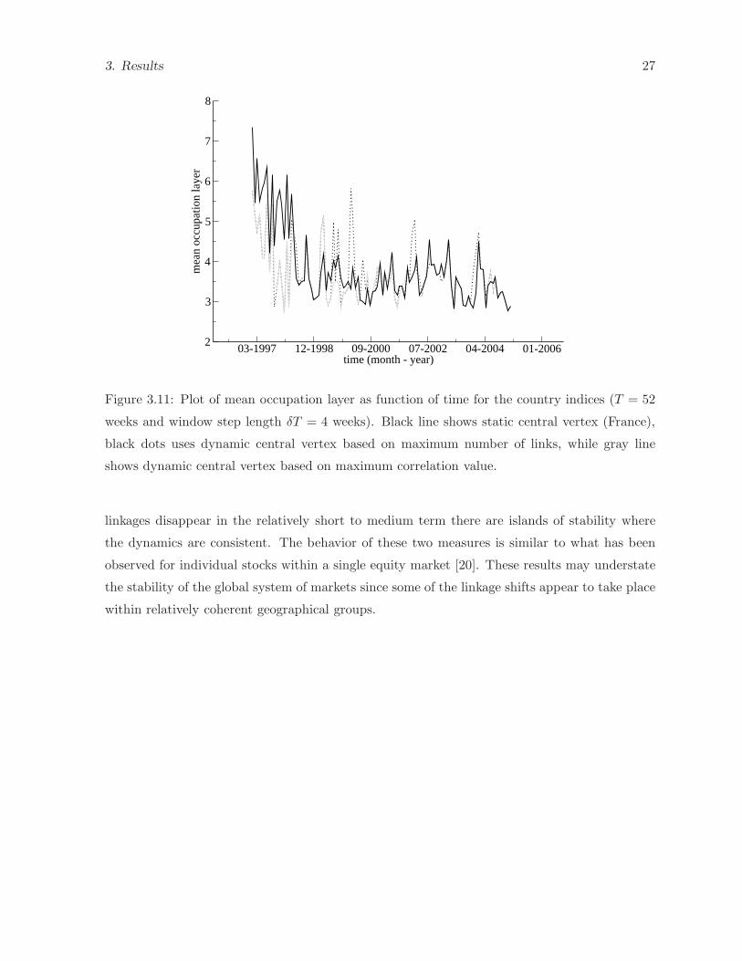
3.3.2 Mean Occupation Layer
The mean occupation layer can be calculated using either a fixed central node for all windows,
i.e., France, or with a continuously updated node. In Figure 3.11 the results are shown for
France as the fixed central node (black line), the dynamic maximum vertex degree node (black
dots) and the dynamic highest correlation vertex (gray line). The three sets of calculations are
roughly consistent. The mean occupation layer fluctuates over time as changes in the MST
occur due to market forces. There is, however, a broad downward trend in the mean occupation
layer, indicating that the MST over time is becoming more compact.
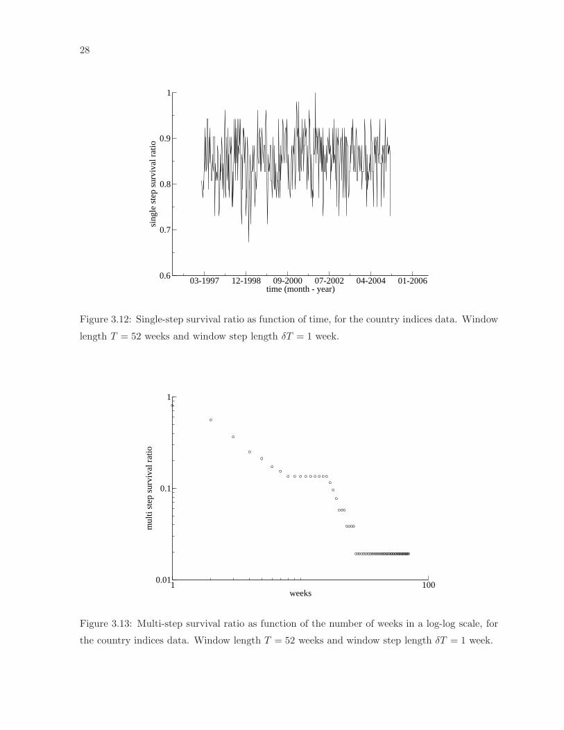
3.3.3 Single and Multi Step Survival Rates
Figure 3.12 presents the single-step survival ratios for the MST of country indices. The average
is about 0.85, indicating that a large majority of links between markets survives from one
window to the next. As might be expected, the ratio increases with increases in window length.
Figure 3.13 shows the multi-step survival ratio. In both cases we used T = 52 weeks and
δT = 1 week. Here, as might be expected, the connections disappear quite rapidly, but a small
proportion of links remains intact, creating a stable base for construction of the MST. Again
the evidence here is of importance for the construction of portfolios, indicating that while most
3. Results 27
03-1997 12-1998 09-2000 07-2002 04-2004 01-2006time (month - year)
2
3
4
5
6
7
8
mea
n oc
cupa
tion
laye
r
Figure 3.11: Plot of mean occupation layer as function of time for the country indices (T = 52
weeks and window step length δT = 4 weeks). Black line shows static central vertex (France),
black dots uses dynamic central vertex based on maximum number of links, while gray line
shows dynamic central vertex based on maximum correlation value.
linkages disappear in the relatively short to medium term there are islands of stability where
the dynamics are consistent. The behavior of these two measures is similar to what has been
observed for individual stocks within a single equity market [20]. These results may understate
the stability of the global system of markets since some of the linkage shifts appear to take place
within relatively coherent geographical groups.
28
03-1997 12-1998 09-2000 07-2002 04-2004 01-2006time (month - year)
0.6
0.7
0.8
0.9
1
sing
le s
tep
surv
ival
rat
io
Figure 3.12: Single-step survival ratio as function of time, for the country indices data. Window
length T = 52 weeks and window step length δT = 1 week.
1 100weeks
0.01
0.1
1
mul
ti st
ep s
urvi
val r
atio
Figure 3.13: Multi-step survival ratio as function of the number of weeks in a log-log scale, for
the country indices data. Window length T = 52 weeks and window step length δT = 1 week.

Chapter 4
Forward Plan
Future work can be divided in four main parts:
• Analytical study of moments and other parameters using the one-factor model and the
multifactor model. Multifactor model with intra-sector and inter-sector terms. One term
is just related with the correlations between stocks of the same sector and the other with the
correlations of stocks from different sectors. Explaining the correlation between moments
of correlations and distances in the MST and the MST arrangement in clusters. Derive the
equation for the spectrum of eigenvalues of the correlation matrix for multifactor models.
• Study of large amount of data of daily stock prices from different markets. How these
stocks will cluster is the main propose of this study. In our studies we saw that stocks
from the same market (London Stock Exchange, FTSE100) clustered together in terms of
industrial sectors, and that indices from different countries cluster in terms of geographical
distance. Now we want to now if the geographical distance is more important that the
industrial classification.
• Simulation of stock prices using a new model, based on our studies of multifactor models,
for the return of the price of a stock. We want to create a new stochastic model for the
returns and compare the results with our empirical data.
• Simulation of a wealth distribution model, with dynamical networks, with few parameters,
that will mimic the real results of a Pareto’s Law with an exponent between 1.5 and 2.5.
This model should be able to get a distribution of wealth with double Pareto tail, as
we can see in many different results of empirical data, a Pareto exponent for the richest
individuals, and another exponent for the few very rich that normally appear in the top
richest list, like Forbes.
29

30
Table 4.1: Gantt chart.Apr May Jun Jul Aug Sep Oct Nov Dec Jan Feb Mar Apr
07 07 07 07 07 07 07 07 07 08 08 08 08
Analytical study of one-factor and multifactor models
Explain correlation between moments of correlations
Spectrum of eigenvalues of correlation matrix
Parameters of the MSTs
Stocks from different markets
MST analysis
Random Matrix Theory analysis
Simulation of a model of returns of stocks
Development and implementation of a new model
Simulations of the model
Simulations of a new Wealth Model
Writing Thesis

Appendix A
Computation of parameters of
T-student distribution
To compute the parameters of a T-student distribution we have to take in account the fact that
some moments of the distribution might not exist, because they diverge, so we use fractional
moments to avoid problems. If we consider:
< SF∓1 >=1
T
T∑
t=1
|R(t)|F∓1 (A-1)
as a fractional moment of the distribution of the returns R(t) because F is a fractional number,
and we compute the rate of the moments as:
rF =< SF−1 >
< SF+1 >=
1
(2k − 3)σ2
[
(k − 1)2
F
]
− 1
(2k − 3)σ2(A-2)
for different exponents in the interval: 23 < F < 1, we can see that rF = a 1
F + b is a linear
function of the parameters, so we can take the values of σ and k from the linear regression:
k =2a − b
2a(A-3)
and
σ2 =1
a + b(A-4)
31

32

Appendix B
Classification and legend for the
industrial sectors of FTSE100 and
the world indices
The classification used for the industrial sectors of FTSE100 is the new classification adopted
by FTSE since the beginning of 2006, the Industry Classification Benchmark [70] created by
Dow Jones Indexes and FTSE. This classification is divided into 10 Industries, 18 Supersec-
tors, 39 Sectors and 104 Subsectors. Our portfolio is composed of 10 industries and 28 sectors:
Oil & Gas (Oil & Gas Producers), Basic Materials (Chemicals, Mining), Industrials (Construc-
tion & Materials, Aerospace & Defence, General Industrials, Industrial Transportation, Support
Services), Consumer Goods (Beverages, Food Producers, Household Goods, Tobacco), Health
Care (Health Care Equipment & Services, Pharmaceuticals & Biotechnology), Consumer Ser-
vices (Food & Drug Retailers, General Retailers, Media, Travel & Leisure), Telecommunications
(Fixed Line Telecommunications, Mobile Telecommunications), Utilities (Electricity, Gas Water
& Multiutilities), Financials (Banks, Nonlife Insurance, Life Insurance, Real Estate, General
Financial, Equity Investment Instruments, Nonequity Investment Instruments) and Technology
(Software & Computer Services). We represent each industry by a symbol: Oil & Gas (�), Basic
Materials (△), Industrials (�), Consumer Goods (grey �), Health Care (�), Consumer Services
(N), Telecommunications (♦), Utilities (•), Financials (grey ◦) and Technology (◦).The coding for the world indices is: Europe, grey circles (grey ◦); North America, white
diamonds (♦); South America, grey squares (grey �); Asian-Pacific area, black triangles (N);
and “other” (Israel, Jordan, Turkey, South Africa), white squares (�).
33

34

Appendix C
List of Publications and
Presentations
Publications
• “A Review of Empirical Studies and Models of Income Distributions in Society”, P. Rich-
mond, S. Hutzler, R. Coelho and P. Repetowicz, in “Econophysics and Sociophysics:
Trends and Perspectives”, eds. Chakrabarti et al., Wiley-VCH (2006)
• “Comments on recent studies of the dynamics and distribution of money”, Peter Richmond,
Przemek Repetowicz, Stefan Hutzler and Ricardo Coelho, Physica A 370 (2006) 43-48,
[Proceedings of the International Conference “Econophysics Colloquium”]
• “Sector analysis for a FTSE portfolio of stocks”, R. Coelho, S. Hutzler, P. Repetowicz and
P. Richmond, Physica A 373 (2007) 615-626
• “The Evolution of Interdependence in World Equity Markets - Evidence from Minimum
Spanning Trees”, Ricardo Coelho, Claire G. Gilmore, Brian Lucey, Peter Richmond and
Stefan Hutzler, Physica A 376 (2007) 455-466
Presentations
• “Dynamics of correlations from a FTSE100 portfolio”, Poster presentation in “Physics of
socio-economic Systems (AKSOE)”, Dresden 26th-31st March 2006
• “Minimal Spanning Trees (MST) analysis of random time series from different distribu-
tions”, Oral presentation in COST P10 Workshop “Network dynamics: From structure to
function”, 23rd September 2006, Vienna
35

36
• “Estudo de Mercados Financeiros: Reais vs. Aleatorios”, Oral presentation in Seminario
do Centro de Fısica do Porto, 6th September 2006

Bibliography
[1] R. N. Mantegna and H. E. Stanley, An Introduction to Econophysics: Correlations and
Complexity in Finance. Cambridge University Press, Cambridge (2001)
[2] J.-P. Bouchaud and M. Potters, Theory of Financial Risk and Derivative Pricing. Cam-
bridge University Press, Cambridge (2003)
[3] A. Chatterjee, S. Yarlagadda and B. K. Chakrabarti, Econophysics of Wealth Distributions.
Springer-Verlag, Milan (2005)
[4] A. Chatterjee, S. Yarlagadda and B. K. Chakrabarti, Econophysics and Sociophysics of
Wealth Distributions. Wiley-VCH, Berlin (2006)
[5] L. Bachelier, Theorie de la speculation, Annales scientifiques de l’E.N.S. 3e serie, 17, 21-86
(1900)
[6] P. Gopikrishnan, M. Meyer, L. A. N. Amaral and H. E. Stanley, Inverse cubic law for the
distribution of stock price variations, Eur. Phys. J. B 3, 139 (1998)
[7] P. Gopikrishnan, V. Plerou, L. A. N. Amaral, M. Meyer and H. E. Stanley, Scaling of the
distribution of flutuations of financial market indices, Phys. Rev. E 60, 5305 (1999)
[8] V. Plerou, P. Gopikrishnan, L. A. N. Amaral, M. Meyer and H. E. Stanley, Scaling of the
distribution of price flutuations of individual companies, Phys. Rev. E 60, 6519 (1999)
[9] M. L. Mehta, Random Matrices, Elsevier-Academic Press, Netherlands (2004)
[10] L. Laloux, P. Cizeau, J.-P. Bouchaud and M. Potters, Noise Dressing of Financial Corre-
lation Matrices, Phys. Rev. Lett. 83, 1467 (1999)
[11] V. Plerou, P. Gopikrishnan, B. Rosenow, L. A. N. Amaral and H. E. Stanley, Universal and
Nonuniversal Properties of Cross Correlations in Financial Time Series, Phys. Rev. Lett.
83, 1471 (1999)
37

38
[12] Z. Burda, J. Jurkiewicz and M. A. Nowak, Applications of Random Matrices to Economy
and other Complex Systems, Acta Physica Polonica B 36, 2603-2838 (2005)
[13] P. Gopikrishnan, B. Rosenow, V. Plerou and H. E. Stanley, Quantifying and interpreting
collective behavior in financial markets, Phys. Rev. E 64, 035106 (2001)
[14] V. Plerou, P. Gopikrishnan, B. Rosenow, L. A. N. Amaral, T. Guhr and H. E. Stanley,
Random matrix approach to cross correlations in financial data, Phys. Rev. E 65, 066126
(2002)
[15] R. N. Mantegna, Hierarchical structure in financial markets, Eur. Phys. J. B 11, 193 (1999)
[16] G. Bonanno, F. Lillo and R. N. Mantegna, High frequency cross-correlation in a set of
stocks, Quantitative Finance 1, 96 (2001)
[17] G. Bonanno, G. Caldarelli, F. Lillo, S. Micciche, N. Vandewalle and R. N. Mantegna,
Network of equities in financial markets, Eur. Phys. J. B 38, 363 (2004)
[18] N. Vandewalle, F. Brisbois and X. Tordois, Non-random topology of stock markets, Quan-
titative Finance 1, 372 (2001)
[19] G. Bonanno, G. Caldarelli, F. Lillo and R. N. Mantegna, Topology of correlation-based
minimal spanning trees in real and model markets, Phys. Rev. E 68, 046130 (2003)
[20] J.-P. Onnela, A. Chakraborti, K. Kaski, J. Kertesz and A. Kanto, Dynamics of market
correlations: Taxonomy and portfolio analysis, Phys. Rev. E 68, 056110 (2003)
[21] J.-P. Onnela, A. Chakraborti, K. Kaski, J. Kertesz and A. Kanto, Asset trees and asset
graphs in financial markets, Physica Scripta T106, 48 (2003)
[22] M. McDonald, O. Suleman, S. Williams, S. Howison and N. F. Johnson, Detecting a cur-
rency’s dominance or dependence using foreign exchange network trees, Phys. Rev. E 72,
046106 (2005)
[23] R. Coelho, S. Hutzler, P. Repetowicz and P. Richmond, Sector analysis for a FTSE portfolio
of stocks, Physica A 373, 615 (2007)
[24] R. Coelho, C. G. Gilmore, B. Lucey, P. Richmond and S. Hutzler, The evolution of interde-
pendence in world equity markets-Evidence from minimum spanning trees, Physica A 376,
455 (2007)
[25] J.-P. Onnela, A. Chakraborti, K. Kaski and J. Kertesz, Dynamic asset trees and portfolio
analysis, Eur. Phys. J. B 30, 285 (2002)

Bibliography 39
[26] J.-P. Onnela, A. Chakraborti, K. Kaski and J. Kertesz, Dynamic asset trees and Black
Monday, Physica A 324, 247 (2003)
[27] H. Situngkir and Y. Surya, On Stock Market Dynamics through Ultrametricity of Minimum
Spanning Tree, Technical Report WPH2005 Bandung Fe Institute, Dept. Computational
Sociology, Bandung Fe Institute (2005)
[28] H. Situngkir and Y. Surya, Tree of Several Asian Currencies, BFI Working Paper No. WPI
2005 (2005)
[29] S. Micciche, G. Bonanno, F. Lillo and R. N. Mantegna, Degree stability of a minimum
spanning tree of price return and volatility, Physica A 324, 66 (2003)
[30] J.-P. Onnela, K. Kaski and J. Kertesz, Clustering and information in correlation based
financial networks, Eur. Phys. J. B 38, 353 (2004)
[31] R.L. Axtell, Zipf Distribution of U.S. Firm Sizes, Sience 293, 1818 (2001)
[32] C. Di Guilmi, E. Gaffeo and M. Gallegati, Power Law Scaling in the World Income Distri-
bution, Economics Bulletin 15, 1 (2003)
[33] V. Pareto, Cours d’Economie Politique, Libraire Droz (Geneve), (1964), new edition of the
original from (1897)
[34] P. Richmond, P. Repetowicz, S. Hutzler and R. Coelho Comments on recent studies of the
dynamics and distribution of money, Physica A 370, 43 (2006)
[35] P. Richmond, S. Hutzler, R. Coelho and P. Repetowicz, A review of empirical studies and
models of income distributions in society, in Econophysics and Sociophysics of Wealth Dis-
tributions. (eds. A. Chatterjee, S. Yarlagadda and B. K. Chakrabart), Wiley-VCH, Berlin
(2006)
[36] O. Malcai, O. Biham, P. Richmond, and S. Solomon, Theoretical analysis and simulations
of the generalized Lotka-Volterra model, Phys Rev E 66, 031102 (2002)
[37] A. Chatterjee, B. K. Chakrabarti and S. S. Manna, Pareto law in a kinetic model of market
with random saving propensity, Physica A 335, 155 (2004)
[38] P. Repetowicz, S. Hutzler and P. Richmond, Dynamics of money and income distributions,
Physica A 356, 641 (2005)
[39] R. Coelho, Z. Neda, J. J. Ramasco and M. A. Santos, A family-network model for wealth
distribution in societies, Physica A 353, 515 (2005)

40
[40] http://www.forbes.com
[41] A. Y. Abul-Magd, Wealth distribution in an ancient Egyptian society, Phys. Rev. E 66,
057104 (2002)
[42] H. Aoyama, W. Souma, Y. Nagahara, M. P. Okazaki, H. Takayasu and M. Takayasu,
Pareto’s law for income of individuals and debt of bankrupt companies, Fractals 8, 293
(2000)
[43] Y. Fujiwara, W. Souma, H. Aoyama, T. Kaizoji and M. Aoki, Growth and fluctuations of
personal income, Physica A 321, 598 (2003)
[44] W. Souma, Universal structure of the personal income distribution, Fractals 9, 463 (2001)
[45] A. Chatterjee, B. K. Chakrabarti and S. S. Manna, Money in Gas-Like Markets: Gibbs and
Pareto Laws, Physica Scripta T106, 36 (2003)
[46] A. Dragulescu and V. M. Yakovenko, Evidence for the exponential distribution of income
in the USA, Eur. Phys. J. B 20, 585 (2001)
[47] A. Dragulescu and V. M. Yakovenko, Exponential and power-law probability distributions
of wealth and income in the United Kingdom and the United States, Physica A 299, 213
(2001)
[48] A. Dragulescu and V. M. Yakovenko, Statistical Mechanics of Money, Income, and Wealth:
A Short Survey, AIP Conference Proceedings 661, 180 (2003)
[49] F. Clementi and M. Gallegati, Power law tails in the Italian personal income distribution,
Physica A 350, 427 (2005)
[50] T. Di Matteo, T. Aste and S. T. Hyde, Exchanges in complex networks: income and wealth
distributions, in The Physics of Complex Systems (New Advances and Perspectives), (eds.
F. Mallamace and H. E. Stanley), IOS Press, Amsterdam (2004)
[51] W. J. Reed, The Pareto law of incomes - an explanation and an extension, Physica A 319,
469 (2003)
[52] N. Scafetta, S. Picozzi and B. J. West, An out-of-equilibrium model of the distributions of
wealth, Quantitative Finance 4, 353 (2004)
[53] G. Willis and J. Mimkes, Evidence for the Independence of Waged and Unwaged Income,
Evidence for Boltzmann Distributions in Waged Income, and the Outlines of a Coherent
Theory, Microeconomics 0408001, EconWPA (2004)

Bibliography 41
[54] S. Sinha, Evidence for power-law tail of the wealth distribution in India, Physica A 359,
555 (2006)
[55] M. Levy and S. Solomon, New evidence for the power-law distribution of wealth, Physica A
242, 90 (1997)
[56] S. Levy, Wealthy People and Fat Tails: An Explanation for the Levy Distribution of Stock
Returns, Finance, 30 (1998)
[57] M. Levy, Are rich people smarter?, J. Econ. Theory 110, 42 (2003)
[58] R. Coelho, Modelos de Distribuicao de Riqueza, MSc Thesis - Universidade do Porto, Porto
(2004)
[59] http://finance.yahoo.com/
[60] http://www.mysql.com/
[61] H. Kleinert, Path Integrals in Quantum Mechanics, Statistics, Polymer Physics and Finan-
cial Markets. World Scientific Publishing, Singapore (2004)
[62] C. Tsallis, C. Anteneodo, L. Borland and R. Osorio, Nonextensive statistical mechanics and
economics, Physica A 324, 89 (2003)
[63] A. M. Sengupta and P. P. Mitra, Distributions of singular values for some random matrices,
Phys. Rev. E 60, 3389 (1999)
[64] W. F. Sharpe, Capital Asset Prices: A Theory of Market Equilibrium under Conditions of
Risk, The Journal of Finance 19, 425 (1964)
[65] F. Lillo and R. N. Mantegna, Spectral density of the correlation matrix of factor models: A
random matrix theory approach, Phys. Rev. E 72, 016219 (2005)
[66] D.-H. Kim and H. Jeong, Systematic analysis of group identification in stock markets, Phys.
Rev. E 72, 046133 (2005)
[67] R. C. Prim, Shortest connection networks and some generalisations, Bell System Tech. J.
36, 1389 (1957)
[68] V. Batagelj and A. Mrvar, Pajek - Program for Large Network Analysis,
http://vlado.fmf.uni-lj.si/pub/networks/pajek/
[69] T. Kamada and S. Kawai, An algorithm for drawing general undirected graphs, Information
Processing Letters 31, 7 (1989)

42
[70] http://www.icbenchmark.com/