Hazem Al Bermanei

Applications of Max-Plus Algebra to Scheduling

Hazem

Al B

ermanei /

/ Ap

plicatio

ns of M

ax-Plus Alg

ebra to

Scheduling

// 2

02

1

ISBN 978-951-765-982-6

9 789517 659826

Hazem Al BermaneiBorn 1966

Previous studies and degreesLicentiate of Science in Applied Mathematics, Åbo Akademi University, 2012 Master of Science in Mathematics, South-Bank University in London, 1997Bachelor of Science in Mathematics, University of Baghdad, 1990

Åbo Akademi University Press Tavastgatan 13, FI-20500 Åbo, Finland Tel. +358 (0)2 215 4793 E-mail: forlaget@abo.fi

Sales and distribution: Åbo Akademi University Library Domkyrkogatan 2–4, FI-20500 Åbo, Finland Tel. +358 (0)2 -215 4190 E-mail: publikationer@abo.fi

APPLICATIONS OF MAX-PLUS ALGEBRA TO SCHEDULING

Applications of Max-Plus Algebra to Scheduling

Hazem Al Bermanei

Åbo Akademis förlag | Åbo Akademi University PressÅbo, Finland, 2021

CIP Cataloguing in Publication

Al Bermanei, Hazem.Applications of max-plus algebra to scheduling / Hazem Al Bermanei. - Åbo : Åbo Akademi University Press, 2021.Diss.: Åbo Akademi University.ISBN 978-951-765-982-6

ISBN 978-951-765-982-6ISBN 978-951-765-983-3 (digital)

Painosalama OyÅbo 2021

v

Preface

There are some people that I would like to thank for their contribution to this thesis and to the research

that will be provided by it.

First, I want to express my gratitude and appreciation to my supervisors Prof. Göran Högnäs, who

has introduced me to the area of max-plus algebra and discrete event systems and Dr. Jari Böling. I

am most grateful for his infinite patience, which is more than I deserved. I want to thank them both

especially for their contagious enthusiasm and creativity, for the pleasant and fruitful cooperation, for

the support and the guidance they have given me during this project, and for the fact that they have

encouraged me to continue my research on this topic.

I am also grateful to my colleagues for their support and assistance for scientific advice both at the

theoretical and practical level.

Furthermore, I would like to express my gratitude to my family (wife and children), my mother, my

brothers and the other members of my family that have supported and encouraged me during the

realization of this thesis.

Finally, I would also like to thank my friends for their support and encouragement.

vi

vii

Abstract

Max-plus algebra provides mathematical theory and techniques for solving nonlinear problems that

can be given the form of linear problems, when arithmetical addition is replaced by the operation of

maximum and arithmetical multiplication is replaced by addition. Problems of this kind are

sometimes of a managerial nature, arising in areas such as manufacturing, transportation, allocation

of resources and information processing technology. Max-plus algebra also provides the linear-

algebraic background to the rapidly developing field of tropical mathematics.

The aim of this thesis is to provide an introductory text to max-plus algebra and to present results on

advanced topics and, in particular, how it is useful in applications. An overview of the basic notions

of the max-plus algebra and max-plus linear discrete event systems (DES) is presented.

Train networks can be modelled as a directed graph, in which nodes correspond to arrivals and

departures at stations, and arcs to traveling times. A particular difficulty is represented by meeting

conditions in a single-track railway system. The stability and sensitivity of the timetable is analyzed,

and different types of delays and delay behavior are discussed. Interpretation of the recovery matrix

is also done. A simple train network with real-world background is used for illustration. Compared

to earlier work, which typically includes numerical optimization, this study is fully done by using

max-plus algebra.

In this thesis, the scheduling of production systems consisting of many stages and different units is

considered, where some of the units can be used for various stages. If a production unit is used for

various stages cleaning is needed in between, while no cleaning is needed between stages of the same

type. Cleaning of units takes a significant amount of time, which is considered in the scheduling. The

goal is to minimize the total production time, and such problems are often solved by using numerical

optimization. In this thesis, the possibilities for using max-plus for the scheduling are investigated.

Structural decisions, such as choosing one unit over another, proved to be difficult. Scheduling of a

small production system consisting of 6 stages and 6 units is used as a case study.

viii

Traffic systems, computer communication systems, production lines, and flows in networks are all

based on discrete event systems and, thus, can be conveniently described and analyzed by means of

max-plus algebra. Max-plus formalism can be used for modeling of train network and production

systems.

ix

Svensk sammanfattning

Max-plusalgebran tillhandhåller matematisk teori och teknik för lösning av icke-linjära problem som

kan ges linjär form genom att vanlig aritmetisk addition ersätts av maximumoperationen medan

aritmetisk multiplikation ersätts av addition. Problem av detta slag är ofta av organisatorisk natur. De

uppträder på områden som tillverkningsindustri, transport, resurstilldelning och

informationsbehandling. Maxalgebran utgör även den linjär-algebraiska bakgrunden till det snabbt

växande området tropisk matematik.

Ändamålet med denna avhandling är att tillhandahålla en inledning till max-plusalgebran och

presentera resultat av mer avancerad natur och i synnerhet visa hur den är användbar i tillämpningar.

Grundbegreppen i max-plusalgebran och teorin för maxpluslinjära händelsedrivna system (Discrete

Event Systems, DES) presenteras.

Tågnätverk kan modelleras som en orienterad graf där noderna representerar ankomster till och

avgångar från stationer, medan kanterna svarar mot restider mellan stationerna. En speciell svårighet

innebär modelleringen av enspåriga tågsystem där tåg gående i olika riktningar måste mötas. En

tågtidtabells stabilitet och känslighet diskuteras, liksom olika typer av förseningar och strategier för

att korrigera dessa. Återställningsmatrisen presenteras och tolkningen av den diskuteras. Teorin

illustreras med hjälp av ett enkelt tågnätverk med verklighetsbakgrund.

En viktig tillämpning är tidsoptimeringen av produktionssystem bestående av många olika stadier

och olika produktionsenheter (maskiner). Av enheterna kan en del användas för olika stadier i

processen. I så fall måste de dock rengöras mellan de olika produktionsskedena. Däremot krävs ingen

rengöring om enheten inte byter uppgift. Rengöringen tar en viss tid som måste beaktas i

modelleringen. Målet är att minimera den totala produktionstiden. Detta har i litteraturen oftast gjorts

med numerisk optimering. I denna avhandling har möjligheten att använda maxplusteknik

undersökts. Strukturella beslut, såsom att besluta vid vilken tidpunktbyte av uppgift (och rengöring)

ska göras, visade sig svåra att direkt modellera som ett maxplusproblem. För hela

produktionsprocessen utvecklades därför ett hybridsystem med maxplusalgebraiska subproblem som

x

central ingrediens. Tidtabellen för ett litet produktionssystem med 6 produktionsskeden och 6

produktionsenheter illustrerar tekniken.

Trafiksystem, datakommunikationssystem, produktionssystem och nätverksflöden baserar sig på

DES och kan därför med fördel beskrivas och analyseras med hjälp av max-plusalgebra.

xi

Outline of the Thesis

The thesis starts in Chapter 1 with an introduction to max-plus algebra. More specifically, we

introduce the basic algebraic concepts and properties of max-plus algebra. The emphasis of the

chapter is on modeling issues, that is, we will discuss what kind of discrete event systems can be

modeled by max-plus algebra.

Chapter 2 deals with three different parts, part one deals with solvability of linear systems such as

𝐴𝐴⨂𝑥𝑥 = 𝑏𝑏 and linear independence and dependence, part two with max-plus linear equations, finding

the eigenvalues and eigenvectors by different methods (maximum cycle mean method and power

method) and part three deals with max-plus linear discrete event systems and a real application,

namely problems in railway networks and simple manufacturing systems. Analogue to characteristic

equation and the Cayley–Hamilton theorem in max-plus algebra are introduced.

Chapter 3 discusses modeling and scheduling of a train network that can be modelled as a directed

graph, in which vertices correspond to arrivals and departures at stations, and arcs to traveling times.

A particular difficulty is represented by meeting conditions in a single-track railway system.

Compared to earlier work which typically includes numerical optimization, max-plus formalism is

used throughout this chapter. The stability and sensitivity of the timetable is analyzed, and different

types of delays and delay behavior are discussed and simulated. Interpretation of the recovery matrix

is also done. A simple train network with real-world background is used for illustration.

In Chapter 4, the scheduling of production systems consists of many stages and different units are

considered, where some of the units can be used for multiple stages. If a production unit is used for

different stages, cleaning is needed in between, while no cleaning is needed between stages of the

same type. Cleaning of units takes a significant amount of time, which is considered in the scheduling.

The goal is to minimize the total production time, and such problems are often solved by using

numerical optimization. In this chapter, max-plus formalism is used for modeling of such production

systems, and the possibilities for using max-plus for the scheduling are also investigated. Structural

decisions such as choosing one unit over another proved to be difficult. Scheduling of a small

production system consisting of 6 stages and 6 units is used as a case study.

xii

Chapter 5 reviews various stochastic extensions and the ergodic theory for stochastic max-plus linear

systems. The common approaches are discussed, and the chapter may serve as a reference to max-

plus ergodic theory.

Chapter 6 discusses the general conclusion.

xiii

List of Publications

This thesis is written as a monograph, but two chapters of it are related to the following manuscripts

Al Bermanei H, Böling JM, and Högnäs G (2016), Modeling and simulation of train networks

using max-plus algebra. The 9th EUROSIM Congress on Modelling and Simulation EUROSIM

2016, Oulu, Finland, DOI: 10.3384/ecp17142: pp. 612-618.

Al Bermanei H, Böling JM, and Högnäs G (2017), Modeling and scheduling of production

system by using max-plus algebra. International Conference on Innovative Technologies (In-

Tech 2017), Ljubljana, Slovenia, Vol. 4, SI-1291: pp.37-40. Awarded for science technology

transfer at the conference (awarded one of the three best articles at the conference).

xiv

xv

List of Symbols

𝜙𝜙 the empty set

𝑁𝑁 set of natural numbers: 𝑁𝑁 = 0, 1, 2, … …

𝑍𝑍 set of integers

𝑄𝑄 set of rational numbers

ℝ set of real numbers

𝐶𝐶 set of complex numbers

𝑃𝑃𝑛𝑛 set of permutations of the set 1, 2, … … . ,𝑛𝑛

𝑃𝑃𝑛𝑛𝑒𝑒 set of even permutations of the set 1, 2, … … . ,𝑛𝑛

𝑃𝑃𝑛𝑛𝑜𝑜 set of odd permutations of the set 1, 2, … … . ,𝑛𝑛

Matrices and Vectors

ℝ𝑚𝑚×𝑛𝑛 set of the m by n matrices with real entries

ℝ𝑛𝑛 set of real column vectors with n components

𝐴𝐴𝑇𝑇 transpose of the matrix A

𝐼𝐼𝑛𝑛 n by n identity matrix

𝑎𝑎𝑖𝑖 ith component of the vector 𝑎𝑎

𝑎𝑎𝑖𝑖𝑖𝑖 , (𝐴𝐴)𝑖𝑖𝑖𝑖 entry of the matrix A on the ith row and the jth column

Max-Plus Algebra

⨁ max-algebraic addition

⨂ max-algebraic multiplication

𝜀𝜀 zero element in a semiring; in the max-plus semiring 𝜀𝜀 = −∞ 𝑒𝑒 unit element in a semiring; in the max-plus semiring 𝑒𝑒 = 0

𝑥𝑥⨂𝑛𝑛 max-algebraic power of x

𝐼𝐼𝑛𝑛 n by n max-algebraic Identity matrix

𝜀𝜀𝑚𝑚⨂𝑛𝑛 m by n max-algebraic zero matrix

𝐴𝐴⨂𝑛𝑛 nth max-algebraic power of the matrix 𝐴𝐴

xvi

ℝmax max-plus algebra: ℝ𝑚𝑚𝑚𝑚𝑚𝑚 = ℝ⋃−∞ 𝐺𝐺(𝐴𝐴) precedence graph of the matrix A 𝑛𝑛 the set 1, … … . ,𝑛𝑛 for 𝑛𝑛 ∈ 𝑁𝑁\0

𝜆𝜆 the eigenvalue and in the stochastic case the Lyapunov exponent of 𝐴𝐴(𝑘𝑘): 𝑘𝑘𝑘𝑘𝑁𝑁

𝜆𝜆 𝑡𝑡𝑜𝑜𝑡𝑡 the top Lyapunov exponent of 𝐴𝐴(𝑘𝑘): 𝑘𝑘𝑘𝑘𝑁𝑁

𝜆𝜆 𝑏𝑏𝑜𝑜𝑡𝑡 the bottom Lyapunov exponent of 𝐴𝐴(𝑘𝑘):𝑘𝑘𝑘𝑘𝑁𝑁

||𝐴𝐴||max the maximal finite element of matrix 𝐴𝐴

||𝐴𝐴||min the minimal finite element of matrix 𝐴𝐴

xvii

Contents

Preface ..................................................................................................................................... v

Abstract ................................................................................................................................ vii

Svensk sammanfattning ....................................................................................................... ix

Outline of the Thesis ............................................................................................................ xi

List of Publications ............................................................................................................. xiii

List of Symbols...................................................................................................................... xv

Contents .............................................................................................................................. xvii

Chapter 1

Introduction ............................................................................................................................ 1

1.1 Brief History of Max-plus ............................................................................................................ 1

1.2 Definitions and Basic Properties ................................................................................................. 5

1.3 Matrices and Vectors in Max-plus Algebra ............................................................................... 7

1.3.1 Matrices ............................................................................................................................... 7

1.3.2 Properties of Matrix Operations .......................................................................................... 9

1.3.3 Vectors ............................................................................................................................... 13

1.4 Matrices and Graphs ................................................................................................................. 14

1.4.1 Matrices and Digraphs ....................................................................................................... 16

Chapter 2

Max-plus Linear Equations ................................................................................................. 19

2.1 Solution of 𝑨𝑨⨂𝒙𝒙 = 𝒃𝒃 ................................................................................................................. 19

2.2 Eigenvalues and Eigenvectors ................................................................................................... 26

2.2.1 Existence and Uniqueness ................................................................................................. 26

xviii

2.2.2 Power Method [12] ............................................................................................................ 32

2.3 Modeling Issue ............................................................................................................................ 40

2.4 Max-plus Linear Discrete Event Systems ................................................................................ 42

2.4.1 Max-plus Linear State Space Models ................................................................................ 42

2.4.2 Example of Simple Production System ............................................................................. 44

2.5 An Introduction to Max-plus Algebraic System Theory ........................................................ 48

2.6 Characteristic Equation and the Cayley-Hamilton Theorem ................................................ 52

2.6.1 Notations and Definitions .................................................................................................. 52

2.6.2 The Characteristic Equation in Ordinary Linear Algebra.................................................. 53

2.6.3 The Characteristic Equation in Max-plus Algebra ............................................................ 54

Chapter 3

Modeling and Scheduling of Train Network ..................................................................... 59

3.1 An Example of Scheduled Max-plus Linear Systems ............................................................. 60

3.2 Delay Sensitivity Analysis .......................................................................................................... 64

3.3 Dynamic Delay Propagation ..................................................................................................... 65

3.4 Recovery Matrix ......................................................................................................................... 66

3.5 Conclusion ................................................................................................................................... 69

Chapter 4

Modeling and Scheduling of Production Systems ............................................................. 71

4.1 Manufacturing System .............................................................................................................. 72

4.1.1 A Max-plus Model for the Production System .................................................................. 73

4.2 Production Schedule from Iteration of the State Equation.................................................... 76

4.3 Asymptotic Case ......................................................................................................................... 78

4.4 Asymptotic Case Using Max-plus ............................................................................................. 84

4.4.1 Production of A, B, and C, M1 .......................................................................................... 84

4.4.2 Production of D and E Using Only One of the Units for D, M2 ....................................... 85

4.4.3 Production of D and E Using Both Units for D, M3 ......................................................... 86

4.5 Conclusion................................................................................................................................... 89

Chapter 5

Stochastic Max-plus Systems ............................................................................................... 91

5.1 Basic Definitions and Examples ................................................................................................ 91

xix

5.1.1 Petri Nets [1] .................................................................................................................... 100

5.2 The Subadditive Ergodic Theorem ........................................................................................ 113

5.3 Matrices with a Fixed Structure ............................................................................................. 118

5.3.1 Irreducible Matrices ......................................................................................................... 118

5.3.2 Beyond Irreducible Matrices ........................................................................................... 129

5.4 State Reduction for Matrices with Dominant Maximal Cycle ............................................. 130

Chapter 6

General Conclusion ............................................................................................................ 139

References ....................................................................................................................................... 141

1

Chapter 1

Introduction Max-plus algebra has been an active area of study since the 1970’s. Much of the first interest and

motivation in this area of mathematics can be seen in connection to the modeling and simulating of

discrete event systems typically arising in areas involving allocation of resources.

The main motivation for this dissertation is to introduce the fascinating mathematical theory and then

show how max-plus algebra fits naturally into the description and analysis of, e.g., graph theoretical

problems and, in particular, can be used with great efficiency in scheduling applications. To make the

presentation self-contained much introductory material on max-plus algebra is included in the first

two chapters. This part is almost of textbook or lecture notes character. The exposition follows well-

known works such as [1], [6] and [7]. Further references are given throughout the text. Chapter 5 is

a brief introduction to stochastic max-plus systems with examples drawn from the previous material.

Chapter 3 and 4 contain our main contribution. A deeper analysis of two scheduling applications is

made: a train schedule and a production schedule in a manufacturing process, respectively. Even if

the max-plus formalism is an efficient tool, great care must be given to system modeling. In Chapter

4, the final procedure turns out to be an interplay between many different methods with max-plus

algebra in a key role. The proposed procedure is much faster and more versatile than the previously

used optimization methods of [33].

1.1 Brief History of Max-plus

In max-plus algebra, we work with the max-plus semi-ring, which is the ℝmax = ℝ⋃−∞ and the

two binary operations addition ⨁ and multiplication ⨂, which are defined by:

𝑎𝑎⨁𝑏𝑏 = max(𝑎𝑎, 𝑏𝑏) , 𝑎𝑎⨂𝑏𝑏 = 𝑎𝑎 + 𝑏𝑏, for all 𝑎𝑎, 𝑏𝑏 ∈ ℝmax and (−∞) + 𝑎𝑎 = −∞.

Furthermore, let 𝜀𝜀 = −∞ and 𝑒𝑒 = 0, the additive and multiplicative identities respectively. The

operations ⨁ and ⨂ are associative, commutative and distributive as in conventional algebra.

2

Example 1.1

5 ⊕ 3 = max(5, 3) = 5, 5 ⊗ 3 = 5 + 3 = 8

5 ⊕ 𝜀𝜀 = max(5,−∞) = 5, 5 ⊗𝜀𝜀 = 5 + (−∞) = 5 −∞ = −∞ = 𝜀𝜀

5 ⊗ 𝑒𝑒 = 5 + 0 = 5, 5⨁𝑒𝑒 = max (5,0) = 5

𝑒𝑒 ⊕ 3 = max(0, 3) = 3 and 𝑒𝑒 ⊕ (−3) = max(0,−3) = 0 = 𝑒𝑒

Max-plus algebra is one of many idempotent semi-rings, which have been considered in different

fields of mathematics. Another one is min-plus algebra, the ⊕ means minimum and the additive

identity is ∞. We shall here consider max-plus algebra only. It first appeared in 1956 in Kleene's

paper and this paper has found applications in many areas such as mathematical physics, algebraic

geometry, and optimization. It is also used in control theory, machine scheduling, discrete event

processes, queuing systems, manufacturing systems, telecommunication networks, parallel

processing systems and traffic theory. Many equations that are used to describe the behavior of these

applications are nonlinear in conventional algebra but become linear in max-plus algebra. This is the

main reason for its usefulness in various fields. Many of the theorems and techniques used in

conventional linear algebra have counterparts in the max-plus semi-ring. Cuninghame-Green [9],

Gaubert [4, 5], Gondran and Minoux [39] are among the researchers who have devoted a considerable

amount of time to create a great deal of the max-plus linear algebra theory we have today. Many of

Cuninghame-Green’s results are found in [9]. They have studied concepts such as solving systems of

linear equations, the eigenvalue problem, and linear independence in the max-plus sense.

In the coming chapters, we shall notice the extent to which max-plus algebra is an analogue of

traditional linear algebra and look at many max-plus counterparts of conventional results.

Example 1.2 Consider the railroad network between two cities [2]. This is an example of how max-

plus algebra can be applied to a discrete event system. Assume we have two cities, S1 being the station

in the first city, and S2 the station in the second city. This system contains 4 trains. The time it takes

a train to go from S1 to S2 is 3 hours where the train travels along track 1. It takes 5 hours to go from

S2 to S1 where the train travels along track 2. These tracks can be referred to as long-distance tracks.

There are two more tracks in this network, one of which runs through city 1 and one of which runs

through city 2. We can refer to these as the inner-city tracks. Call them tracks 3 and 4 respectively.

We can picture track 3 as a loop beginning and ending at S1. Similarly, track 4 starts and ends at S2.

The time it takes to traverse the loop on track 3 is 2 hours. The time it takes to travel from S2 to S2 on

track 4 is 3 hours. Track 3 and track 4 each contains a train. Two trains circulate along the two long-

distance tracks. In this network, we also have the following criteria:

3

1. The travel times along each track indicated above are fixed

2. The frequency of the trains must be the same on all four tracks

3. Two trains must leave a station simultaneously in order to wait for the changeover of

passengers

4. The two (𝑘𝑘 + 1)𝑠𝑠𝑡𝑡 trains leaving Si cannot leave until the kth train that left the other station

arrives at Si.

𝑥𝑥𝑖𝑖(𝑘𝑘 − 1) will denote the kth departure time for the two trains from station i. Therefore, 𝑥𝑥1(𝑘𝑘) denotes

the departure time of the pair of 𝑘𝑘 + 1 trains from S1 and 𝑥𝑥2(𝑘𝑘) is the departure time of the 𝑘𝑘 + 1

trains from S2. 𝑥𝑥(0) is a vector denoting the departure times of the first trains from S1 and S2. Thus,

𝑥𝑥1(0) denotes the departure time of the first pair of trains from station 1 and likewise 𝑥𝑥2(0) denotes

the departure time of the first pair of trains from station 2 [2]. See Figure 1.1.

Figure 1.1: Train problem

If we want to determine the departure time of the kth trains from station 1, then we can see that

𝑥𝑥1(𝑘𝑘 + 1) ≥ 𝑥𝑥1(𝑘𝑘) + 𝑎𝑎11 + 𝛿𝛿 and

𝑥𝑥1(𝑘𝑘 + 1) ≥ 𝑥𝑥2(𝑘𝑘) + 𝑎𝑎12 + 𝛿𝛿,

where 𝑎𝑎𝑖𝑖𝑖𝑖 denotes the travel time from station j to station i and δ is the time allowed for the passengers

to get on and off the train. Thus, in our situation we have:

𝑎𝑎11 = 2,𝑎𝑎22 = 3,𝑎𝑎12 = 5 and 𝑎𝑎21 = 3.

We will assume δ = 0 in this example. Thus, it follows that

𝑥𝑥1(𝑘𝑘 + 1) = max 𝑥𝑥1(𝑘𝑘) + 𝑎𝑎11, 𝑥𝑥2(𝑘𝑘) + 𝑎𝑎12.

Similarly, we can see that

𝑥𝑥2(𝑘𝑘 + 1) = max 𝑥𝑥1(𝑘𝑘) + 𝑎𝑎21, 𝑥𝑥2(𝑘𝑘) + 𝑎𝑎22.

In conventional algebra we would determine the successive departure times by iterating the nonlinear

system,

𝑥𝑥𝑖𝑖(𝑘𝑘 + 1) = max𝑖𝑖=1,2,…𝑛𝑛

𝑎𝑎𝑖𝑖𝑖𝑖 + 𝑥𝑥𝑖𝑖(𝑘𝑘)

3 s1 s2

3

5

2

4

In max-plus we can write this as:

𝑥𝑥𝑖𝑖(𝑘𝑘 + 1) = ⨁𝑖𝑖=1𝑛𝑛 𝑎𝑎𝑖𝑖𝑖𝑖⨂𝑥𝑥𝑖𝑖(𝑘𝑘) , 𝑗𝑗 = 1,2, … … ,𝑛𝑛,

where

⨁𝑖𝑖=1𝑛𝑛 𝑎𝑎𝑖𝑖𝑖𝑖⨂𝑥𝑥𝑖𝑖(𝑘𝑘) = (𝑎𝑎𝑖𝑖1⨂𝑥𝑥1)⨁(𝑎𝑎𝑖𝑖2⨂𝑥𝑥2)⨁… … . . .⨁(𝑎𝑎𝑖𝑖𝑛𝑛⨂𝑥𝑥𝑛𝑛) for , 𝑖𝑖 = 1,2, … … ,𝑛𝑛.

In the example we have, 𝑥𝑥1(1) = 0 ⊕ 5 = 5 and 𝑥𝑥2(1) = 1 ⊕ 3 = 3, provided we are given

𝑥𝑥1(0) = −2 and 𝑥𝑥2(0) = 0.

Thus, 𝐴𝐴 = 2 5

3 3 and 𝑥𝑥(0) =

−2

0.

We can express this system using matrices and vectors such that 𝑥𝑥(𝑘𝑘) = 𝐴𝐴⨂𝑥𝑥(𝑘𝑘 − 1). So, 𝑥𝑥(1) =

𝐴𝐴⨂𝑥𝑥(0),𝑥𝑥(2) = 𝐴𝐴⨂𝑥𝑥(1) = 𝐴𝐴⨂𝐴𝐴⨂𝑥𝑥(0) = 𝐴𝐴⨂2⨂𝑥𝑥(0). Thus, in general

𝑥𝑥(𝑘𝑘) = 𝐴𝐴⨂𝑘𝑘⨂𝑥𝑥(0).

This gives us a simple example of how a system of equations, which is not linear in the conventional

algebra, is linear in max-plus algebra.

Example 1.3 Consider two flights from airports A and B arriving at a major airport C from which

two other connecting flights depart [20].

Figure 1.2: Transfer between connecting flights

The airport has many gates and the transfer time between them is nontrivial. Departure times from C

are given and cannot be changed; for the above-mentioned flights, they are b1 and b2. The transfer

times between the two arrival and two departure gates are given in the matrix

5

𝐴𝐴 = 𝑎𝑎11 𝑎𝑎12𝑎𝑎21 𝑎𝑎22

.

Durations of the flights from 𝐴𝐴 to 𝐶𝐶 and 𝐵𝐵 to 𝐶𝐶 are d1 and d2, respectively.

The task is to determine the departure times 𝑥𝑥1 and 𝑥𝑥2 from A and B, respectively, so that all

passengers arrive at the departure gates on time, but as close as possible to the closing times (Figure

1.2). We can express the gate closing times in terms of departure times from airports A and B,

𝑏𝑏1 = max(𝑥𝑥1 + 𝑑𝑑1 + 𝑎𝑎11 , 𝑥𝑥2 + 𝑑𝑑2 + 𝑎𝑎12),

𝑏𝑏2 = max(𝑥𝑥1 + 𝑑𝑑1 + 𝑎𝑎21 , 𝑥𝑥2 + 𝑑𝑑2 + 𝑎𝑎22).

In max-plus algebraic notation, this system gets a more concise succinct form of a system of linear

equations: 𝑏𝑏 = 𝐵𝐵⨂𝑥𝑥, and the matrix 𝐵𝐵 = 𝐴𝐴⨂𝑑𝑑 where

𝐴𝐴 = 𝑎𝑎11 𝑎𝑎12𝑎𝑎21 𝑎𝑎22

, 𝑑𝑑 = 𝑑𝑑1 𝜀𝜀

𝜀𝜀 𝑑𝑑2 and 𝑏𝑏 =

𝑏𝑏1𝑏𝑏2.

We will see in Section 2.1 how to solve such systems. For those that have no solution, Section 2.1

provides a simple max-plus algebraic technique for finding the solution to the inequality 𝐵𝐵⨂𝑥𝑥 ≤ 𝑏𝑏.

1.2 Definitions and Basic Properties

In this section we introduce max-plus algebra, give the essential definitions and study the concepts

that play a key role in max-plus.

Definition 1.1 We denote ℝmax = ℝ⋃−∞ and the two binary operations addition ⨁ and

multiplication ⨂, which are defined by:

𝑎𝑎⨁𝑏𝑏 = max(𝑎𝑎, 𝑏𝑏) ,𝑎𝑎⨂𝑏𝑏 = 𝑎𝑎 + 𝑏𝑏, for all 𝑎𝑎, 𝑏𝑏 ∈ ℝmax and (−∞) + 𝑎𝑎 = −∞.

Define 𝜀𝜀 = −∞ and 𝑒𝑒 = 0. The additive and multiplicative identities are, thus, 𝜀𝜀 and 𝑒𝑒 respectively

and the operations are associative, commutative and distributive as in conventional algebra. The

possibility of working in a formally linear way is because the following statements hold for

𝑎𝑎, 𝑏𝑏, 𝑐𝑐 𝑘𝑘ℝmax.

For the addition ⊕

• Commutativity

For all 𝑎𝑎, 𝑏𝑏 ∈ ℝmax, 𝑎𝑎 ⊕ 𝑏𝑏 = max(𝑎𝑎, 𝑏𝑏) = max(𝑏𝑏, 𝑎𝑎) = 𝑏𝑏 ⊕ 𝑎𝑎

6

• Associativity

For all 𝑎𝑎, 𝑏𝑏, 𝑐𝑐 ∈ ℝmax, 𝑎𝑎 ⊕ (𝑏𝑏 ⊕ 𝑐𝑐) = max(𝑎𝑎, ( 𝑏𝑏 ⊕ 𝑐𝑐))

= max(𝑎𝑎(max (𝑏𝑏, 𝑐𝑐)) = max(𝑎𝑎, 𝑏𝑏, 𝑐𝑐)

= max(max (a, b), 𝑐𝑐) = max(𝑎𝑎, 𝑏𝑏) ⊕𝑐𝑐 = (𝑎𝑎 ⊕ 𝑏𝑏) ⊕ 𝑐𝑐

• Zero Element

𝑎𝑎 ⊕ 𝜀𝜀 = max(𝑎𝑎, 𝜀𝜀) = 𝑎𝑎= max(𝜀𝜀,𝑎𝑎) = 𝜀𝜀 ⊕ 𝑎𝑎

• Idempotency of Addition

𝑎𝑎 ⊕ 𝑎𝑎 = 𝑎𝑎

𝑎𝑎 ⊕ 𝑏𝑏 = max( 𝑎𝑎, 𝑏𝑏) = 𝑎𝑎 or 𝑏𝑏

𝑎𝑎 ⊕ 𝑏𝑏 = max( 𝑎𝑎, 𝑏𝑏) ≥ 𝑎𝑎

𝑎𝑎 ⊕ 𝑏𝑏 = 𝑎𝑎 ⟺ 𝑎𝑎 ≥ 𝑏𝑏

For the multiplication ⨂

• Commutativity

For all 𝑎𝑎, 𝑏𝑏 ∈ ℝmax,𝑎𝑎⨂𝑏𝑏 = 𝑎𝑎 + 𝑏𝑏 = 𝑏𝑏 + 𝑎𝑎 = 𝑏𝑏⨂𝑎𝑎

• Associativity

For all 𝑎𝑎, 𝑏𝑏, 𝑐𝑐 ∈ ℝmax,𝑎𝑎⨂(𝑏𝑏⨂𝑐𝑐) = (𝑎𝑎⨂𝑏𝑏)⨂𝑐𝑐

• Unit Element

𝑎𝑎⨂𝑒𝑒 = 𝑎𝑎= 𝑒𝑒⨂𝑎𝑎

• Zero Element

𝑎𝑎⨂𝜀𝜀 = 𝜀𝜀= ε⨂𝑎𝑎

• Multiplicative Inverse

𝑎𝑎⨂𝑎𝑎−1 = 𝑒𝑒 = 𝑎𝑎−1⨂𝑎𝑎 for all 𝑎𝑎 ∈ ℝ

𝑎𝑎⨂𝑎𝑎−1 = 𝑎𝑎 + (−𝑎𝑎) because 𝑎𝑎−1 = −𝑎𝑎 for all 𝑎𝑎 ∈ ℝ

So 𝑎𝑎⨂𝑎𝑎−1 = 𝑒𝑒 = 𝑎𝑎−1⨂𝑎𝑎

Of course, 𝜀𝜀 has no multiplicative inverse

• (a⨁b)⨂𝑐𝑐 = (𝑎𝑎⨂𝑐𝑐) ⊕ (𝑏𝑏⨂𝑐𝑐) Distributive law

Proof: (a⨁b)⨂𝑐𝑐 = max(𝑎𝑎, 𝑏𝑏)⨂𝑐𝑐 = max(𝑎𝑎, 𝑏𝑏) + 𝑐𝑐 = max(𝑎𝑎 + 𝑐𝑐, 𝑏𝑏 + 𝑐𝑐)

= max(𝑎𝑎⨂𝑐𝑐, 𝑏𝑏⨂𝑐𝑐) = (𝑎𝑎⨂𝑐𝑐)⨁(𝑏𝑏⨂𝑐𝑐)

• If 𝑎𝑎 ≥ 𝑏𝑏 ⟹ 𝑎𝑎⨁𝑐𝑐 ≥ 𝑏𝑏⨁𝑐𝑐 and

if 𝑎𝑎 ≥ 𝑏𝑏 ⟹ 𝑎𝑎⨂𝑐𝑐 ≥ 𝑏𝑏⨂𝑐𝑐

• If 𝑎𝑎⨂𝑐𝑐 ≥ 𝑏𝑏 ⨂𝑐𝑐, 𝑐𝑐 ∈ ℝ ⟹ 𝑎𝑎 ≥ 𝑏𝑏 cancellative law

Lemma 1.1: For any 𝑎𝑎 ∈ ℝmax ∖ 𝜀𝜀, a does not have an additive inverse.

7

Proof: Let 𝑎𝑎 ∈ ℝ𝑚𝑚𝑚𝑚𝑚𝑚 and 𝑎𝑎 ≠ 𝜀𝜀 such that a has an inverse with respect to ⊕.

Let 𝑏𝑏 be the inverse of ⟹ 𝑎𝑎⨁𝑏𝑏 = 𝜀𝜀 , adding 𝑎𝑎 to both sides gives,

𝑎𝑎⨁(𝑎𝑎⨁𝑏𝑏) = 𝑎𝑎⨁𝜀𝜀 = 𝑎𝑎, using the associative property of ⊕ gives

𝑎𝑎 = (𝑎𝑎⨁𝑎𝑎)⨁𝑏𝑏 = 𝑎𝑎⨁𝑏𝑏, 𝑎𝑎 is an idempotent, i.e. 𝑎𝑎 ⊕ 𝑎𝑎 = 𝑎𝑎.

Hence 𝑎𝑎 = 𝑎𝑎⨁𝑏𝑏 = 𝜀𝜀 which is contradiction because 𝑎𝑎 ≠ 𝜀𝜀.

Thus, 𝑎𝑎 does not have an additive inverse.

1.3 Matrices and Vectors in Max-plus Algebra

In this section, we are mainly concerned with systems of linear equations. There are two kinds of

linear systems in ℝmax for which we can compute solutions of 𝑦𝑦 = 𝐴𝐴⊗ 𝑥𝑥⊕ 𝑏𝑏. We also study the

spectral theory of matrices. There exist good notions of the eigenvalue and the eigenvector but there

is often only one eigenvalue; this occurs when the precedence graph associated with the matrix is

strongly connected.

1.3.1 Matrices

The set of 𝑛𝑛 × 𝑚𝑚 matrices where 𝑛𝑛,𝑚𝑚 ∈ 𝑁𝑁 over ℝmax, denote by ℝmax𝑚𝑚×𝑛𝑛, where n is the numbers of

rows and m is the number of columns. We write the matrix 𝐴𝐴 ∈ ℝmax𝑚𝑚×𝑛𝑛 as:

𝐴𝐴 =

⎝

⎜⎛𝑎𝑎11 𝑎𝑎12 …

𝑎𝑎21 𝑎𝑎22 …

: : …

𝑎𝑎1𝑛𝑛𝑎𝑎2𝑛𝑛

:𝑎𝑎𝑚𝑚1 𝑎𝑎𝑚𝑚2 … 𝑎𝑎𝑚𝑚𝑛𝑛⎠

⎟⎞

, the entry in the ith row and jth column of A is denoted 𝑎𝑎𝑖𝑖𝑖𝑖

Definition 1.2:

• For all 𝐴𝐴,𝐵𝐵 ∈ ℝmax𝑛𝑛×𝑛𝑛, define their sum by:

(𝐴𝐴⨁𝐵𝐵)𝑖𝑖𝑖𝑖 = 𝑎𝑎𝑖𝑖𝑖𝑖⨁𝑏𝑏𝑖𝑖𝑖𝑖 = max (𝑎𝑎𝑖𝑖𝑖𝑖, 𝑏𝑏𝑖𝑖𝑖𝑖)

• For all 𝐴𝐴 ∈ ℝmax𝑚𝑚×𝑘𝑘,𝐵𝐵 ∈ ℝmax

𝑘𝑘×𝑛𝑛 define their product by:

(𝐴𝐴⨂𝐵𝐵)𝑖𝑖𝑖𝑖 =⊕𝑙𝑙=1𝑘𝑘 𝑎𝑎𝑖𝑖𝑙𝑙⨁𝑏𝑏𝑙𝑙𝑖𝑖 = max

𝑙𝑙=1,2,…,𝑘𝑘𝑎𝑎𝑖𝑖𝑙𝑙 + 𝑏𝑏𝑙𝑙𝑖𝑖

The transpose of the matrix 𝐴𝐴 ∈ ℝmax𝑚𝑚×𝑛𝑛 is, denoted by 𝐴𝐴𝑇𝑇 ∈ ℝmax

𝑛𝑛×𝑚𝑚 and is define as:

[𝐴𝐴𝑇𝑇]𝑖𝑖𝑖𝑖 = [𝐴𝐴]𝑖𝑖𝑖𝑖

• The 𝑛𝑛 × 𝑛𝑛 identity matrix 𝐼𝐼𝑛𝑛 ∈ ℝ𝑚𝑚𝑚𝑚𝑚𝑚𝑛𝑛×𝑛𝑛 in max-plus is defined as:

8

(𝐼𝐼𝑛𝑛)𝑖𝑖𝑖𝑖 = 𝑒𝑒 if 𝑖𝑖 = 𝑗𝑗

𝜀𝜀 if 𝑖𝑖 ≠ 𝑗𝑗

• For 𝐴𝐴 ∈ ℝ𝑚𝑚𝑚𝑚𝑚𝑚𝑛𝑛×𝑛𝑛 , 𝐼𝐼𝑛𝑛⨂𝐴𝐴 = 𝐴𝐴⨂𝐼𝐼𝑛𝑛 = 𝐴𝐴

• The 𝑛𝑛 × 𝑛𝑛 zero matrix 𝜀𝜀𝑛𝑛 ∈ ℝ𝑚𝑚𝑚𝑚𝑚𝑚𝑛𝑛×𝑛𝑛 in max-plus is defined as:

(𝜀𝜀𝑛𝑛)𝑖𝑖𝑖𝑖 = ε for all 𝑖𝑖, 𝑗𝑗

• For a square matrix 𝐴𝐴 and positive integer 𝑛𝑛 the 𝑛𝑛𝑡𝑡ℎ power of 𝐴𝐴 is written as

𝐴𝐴⨂𝑛𝑛 and it is defined by: n times

n A..........AA A ⊗⊗⊗=⊗

• For any matrix 𝐴𝐴 and any scalar ∝∈ ℝmax

[∝ ⨂𝐴𝐴]𝑖𝑖𝑖𝑖 =∝ ⨂[𝐴𝐴]𝑖𝑖𝑖𝑖

Example 1.4: Let 𝐴𝐴,𝐵𝐵 be two 2 × 2 matrices in ℝmax𝑛𝑛×𝑛𝑛 where

𝐴𝐴 = 2 𝑒𝑒

1 3 and 𝐵𝐵 =

3 −1

2 4, so

𝑨𝑨⊕𝑩𝑩 = max( 2,3) max( 𝑒𝑒,−1)

max( 1,2) max( 4,3) =

3 𝑒𝑒

2 4 = 𝑩𝑩⊕𝑨𝑨.

And

𝑨𝑨⊗𝑩𝑩 = (2 ⊗ 3) ⊕ (𝑒𝑒 ⊗ 2) (2 ⊗−1) ⊕ (𝑒𝑒 ⊗ 4)

(1 ⊗ 3) ⊕ (3 ⊗ 2) (1 ⊗−1) ⊕ (3 ⊗ 4)

= max( 2 + 3 , 0 + 2) max( 2 − 1 , 0 + 4)

max( 1 + 3 , 3 + 2) max( 1 − 1 , 3 + 4) =

max( 5,2) max( 1,4)

max( 4,5) max( 0,7)

= 5 4

5 7

But 𝑩𝑩⊗𝑨𝑨 = (3 ⊗ 2) ⊕ (−1⊗ 1) (3 ⊗ 𝑒𝑒) ⊕ (−1 ⊗ 3)

(2 ⊗ 2) ⊕ (4 ⊗ 1) (2 ⊗ 𝑒𝑒) ⊕ (4 ⊗ 3)

= max(3 + 2 , − 1 + 1) max(3 + 0 , − 1 + 3)

max(2 + 2 , 4 + 1) max(2 + 0 , 4 + 3) =

max(5,0) max(3,2)

max(4,5) max(2,7)

= 5 3

5 7 ≠ 𝑨𝑨⊗𝑩𝑩

In general, we can say that for some 𝐴𝐴,𝐵𝐵 ∈ ℝmax𝑛𝑛×𝑛𝑛 ,𝐴𝐴⨂𝐵𝐵 ≠ 𝐵𝐵⨂𝐴𝐴 i.e. ⨂ is not commutative in ℝmax

𝑛𝑛×𝑛𝑛

9

1.3.2 Properties of Matrix Operations

For the matrices, 𝐴𝐴,𝐵𝐵,𝐶𝐶 in ℝmax𝑛𝑛×𝑛𝑛 we have:

For the addition ⊕

• Commutativity

For all 𝐴𝐴,𝐵𝐵 ∈ ℝmax𝑛𝑛×𝑛𝑛 ,𝐴𝐴⨁𝐵𝐵 = 𝐵𝐵⨁𝐴𝐴

• Associativity

For all 𝐴𝐴,𝐵𝐵,𝐶𝐶 ∈ ℝmax𝑛𝑛×𝑛𝑛 , (𝐴𝐴⨁𝐵𝐵)⨁𝐶𝐶 = 𝐴𝐴⨁(𝐵𝐵⨁𝐶𝐶)

• 𝐴𝐴⨁𝜀𝜀 = 𝐴𝐴 = 𝜀𝜀 ⨁𝐴𝐴

• We define ≥ by:

𝐵𝐵 ≥ 𝐴𝐴 if and only if 𝑏𝑏𝑖𝑖𝑖𝑖 ≥ 𝑎𝑎𝑖𝑖𝑖𝑖 for all 𝑖𝑖, 𝑗𝑗

So, 𝐴𝐴⨁𝐵𝐵 ≥ 𝐴𝐴

• 𝐴𝐴⨁𝐵𝐵 = 𝐴𝐴 ⟺ 𝐴𝐴 ≥ 𝐵𝐵

Proof: Let 𝐴𝐴 = 𝑎𝑎𝑖𝑖𝑖𝑖,𝐵𝐵 = 𝑏𝑏𝑖𝑖𝑖𝑖 for all 𝑖𝑖, 𝑗𝑗

1) If 𝐴𝐴⨁𝐵𝐵 = 𝐴𝐴 ⇒ 𝑎𝑎𝑖𝑖𝑖𝑖⨁𝑏𝑏𝑖𝑖𝑖𝑖 = 𝑎𝑎𝑖𝑖𝑖𝑖 for all 𝑖𝑖, 𝑗𝑗

⇒ max(𝑎𝑎𝑖𝑖𝑖𝑖 , 𝑏𝑏𝑖𝑖𝑖𝑖) = 𝑎𝑎𝑖𝑖𝑖𝑖 ⇒ 𝑎𝑎𝑖𝑖𝑖𝑖 ≥ 𝑏𝑏𝑖𝑖𝑖𝑖 ⇒ 𝐴𝐴 ≥ 𝐵𝐵

2) If 𝐴𝐴 ≥ 𝐵𝐵 = 𝐴𝐴 ⇒ 𝑎𝑎𝑖𝑖𝑖𝑖 ≥ 𝑏𝑏𝑖𝑖𝑖𝑖 for all 𝑖𝑖, 𝑗𝑗

⇒ max(𝑎𝑎𝑖𝑖𝑖𝑖 , 𝑏𝑏𝑖𝑖𝑖𝑖) = 𝑎𝑎𝑖𝑖𝑖𝑖 ⇒ 𝑎𝑎𝑖𝑖𝑖𝑖⨁𝑏𝑏𝑖𝑖𝑖𝑖 = 𝑎𝑎𝑖𝑖𝑖𝑖 ⇒ 𝐴𝐴⊕𝐵𝐵 = 𝐴𝐴

For the multiplication ⨂:

• 𝐴𝐴⨂𝐵𝐵 ≠ 𝐵𝐵⨂𝐴𝐴 in general

• Associativity

For all 𝐴𝐴,𝐵𝐵,𝐶𝐶 ∈ ℝmax𝑛𝑛×𝑛𝑛 ,𝐴𝐴⨂(𝐵𝐵⨂𝐶𝐶) = (𝐴𝐴⨂𝐵𝐵)⨂𝐶𝐶

Proof: 𝐴𝐴⨂(𝐵𝐵⨂𝐶𝐶) =⊕𝑘𝑘=1𝑛𝑛 𝑎𝑎𝑖𝑖𝑘𝑘⨂(𝐵𝐵⨂𝐶𝐶)𝑘𝑘𝑖𝑖 = max

1≤𝑘𝑘≤𝑛𝑛𝑎𝑎𝑖𝑖𝑘𝑘⨂(𝐵𝐵⨂𝐶𝐶)𝑘𝑘𝑖𝑖

= max1≤𝑘𝑘≤𝑛𝑛

(𝑎𝑎𝑖𝑖𝑘𝑘 + max1≤𝑘𝑘≤𝑛𝑛

(𝑏𝑏𝑘𝑘𝑘𝑘 + 𝑐𝑐𝑘𝑘𝑗𝑗)

= max 1≤𝑙𝑙≤𝑛𝑛

max1≤𝑘𝑘≤𝑛𝑛

(𝑎𝑎𝑖𝑖𝑘𝑘 + 𝑏𝑏𝑘𝑘𝑙𝑙 + 𝑐𝑐𝑙𝑙𝑖𝑖) = max1≤𝑙𝑙≤𝑛𝑛

max1≤𝑘𝑘≤𝑛𝑛

(𝑎𝑎𝑖𝑖𝑘𝑘 + 𝑏𝑏𝑘𝑘𝑙𝑙) + 𝑐𝑐𝑙𝑙𝑖𝑖

10

= max1≤𝑙𝑙≤𝑛𝑛

(𝐴𝐴⊗𝐵𝐵)𝑖𝑖𝑙𝑙 + 𝑐𝑐𝑙𝑙𝑖𝑖 = (𝐴𝐴⊗𝐵𝐵) ⊗𝐶𝐶

• Unit Matrix

For all 𝐴𝐴, 𝐼𝐼𝑛𝑛 ∈ ℝmax𝑛𝑛×𝑛𝑛 ,𝐴𝐴⨂𝐼𝐼𝑛𝑛 = 𝐴𝐴 = 𝐼𝐼𝑛𝑛⨂𝐴𝐴

• Zero Matrix

For all 𝐴𝐴, 𝜀𝜀𝑛𝑛 ∈ ℝmax𝑛𝑛×𝑛𝑛 ,𝐴𝐴⨂𝜀𝜀𝑛𝑛 = 𝜀𝜀𝑛𝑛 = 𝜀𝜀𝑛𝑛 ⨂𝐴𝐴

Note that 𝜀𝜀𝑛𝑛 is the 𝑛𝑛 × 𝑛𝑛 zero matrix.

• Distributivity

For all 𝐴𝐴,𝐵𝐵,𝐶𝐶 ∈ ℝmax𝑛𝑛×𝑛𝑛 , (𝐴𝐴⨁𝐵𝐵)⨂𝐶𝐶) = (𝐴𝐴⨂𝐶𝐶)⨁(𝐵𝐵⨂𝐶𝐶 and

𝐴𝐴⨂(𝐵𝐵⨁𝐶𝐶) = (𝐴𝐴⨂𝐵𝐵)⨁(𝐴𝐴⨂𝐶𝐶)

Proof: (𝐴𝐴⨁𝐵𝐵)⨂𝐶𝐶)𝑖𝑖𝑖𝑖 =⊕𝑖𝑖=1𝑛𝑛 𝑎𝑎𝑖𝑖𝑖𝑖⨂(max(𝑏𝑏𝑖𝑖𝑖𝑖, 𝑐𝑐𝑖𝑖𝑖𝑖))

= max𝑖𝑖

[max (𝑎𝑎𝑖𝑖𝑖𝑖 + 𝑏𝑏𝑖𝑖𝑖𝑖),(𝑎𝑎𝑖𝑖𝑖𝑖 + 𝑐𝑐𝑖𝑖𝑖𝑖)] = max(max𝑖𝑖

(𝑎𝑎𝑖𝑖𝑖𝑖 + 𝑏𝑏𝑖𝑖𝑖𝑖) + max𝑖𝑖

(𝑎𝑎𝑖𝑖𝑖𝑖 + 𝑐𝑐𝑖𝑖𝑖𝑖))

= max[ (𝐴𝐴⨂𝐵𝐵)𝑖𝑖𝑖𝑖, (𝐴𝐴⨂𝐶𝐶)𝑖𝑖𝑖𝑖] = [(𝐴𝐴⨂𝐵𝐵)⨁(𝐴𝐴⨂𝐶𝐶)]𝑖𝑖𝑖𝑖 = (𝐴𝐴⨂𝐵𝐵)⨁(𝐴𝐴⨂𝐶𝐶)

And for all 𝒂𝒂 ∈ ℝ

i. 𝑎𝑎 ⊗ (𝐵𝐵⊕ 𝐶𝐶) = 𝑎𝑎 ⊗ 𝐵𝐵⊕ 𝑎𝑎⊗ 𝐶𝐶 and

ii. 𝑎𝑎 ⊗ (𝐵𝐵⊗ 𝐶𝐶) = 𝐵𝐵⊗ 𝑎𝑎⊗ 𝐶𝐶

proof: i. 𝑎𝑎 ⊗ (𝐵𝐵⊕ 𝐶𝐶) = 𝑎𝑎 ⊗ max( 𝑏𝑏𝑖𝑖𝑖𝑖 , 𝑐𝑐𝑖𝑖𝑖𝑖) = 𝑎𝑎 + max( 𝑏𝑏𝑖𝑖𝑖𝑖, 𝑐𝑐𝑖𝑖𝑖𝑖) = max(𝑎𝑎 + 𝑏𝑏𝑖𝑖𝑖𝑖, 𝑎𝑎 + 𝑐𝑐𝑖𝑖𝑖𝑖)

= max(𝑎𝑎 ⊗ 𝐵𝐵,𝑎𝑎 ⊗ 𝐶𝐶) = (𝑎𝑎 ⊗ 𝐵𝐵) ⊕ (𝑎𝑎 ⊗ 𝐶𝐶)

ii. 𝑎𝑎 ⊗ (𝐵𝐵⊗ 𝐶𝐶) = 𝑎𝑎 ⊗ (⊕𝑘𝑘=1𝑛𝑛 (𝑏𝑏𝑖𝑖𝑘𝑘 + 𝑐𝑐𝑘𝑘𝑖𝑖) = 𝑎𝑎 ⊗ ( max

1≤𝑘𝑘≤𝑛𝑛(𝑏𝑏𝑖𝑖𝑘𝑘 + 𝑐𝑐𝑘𝑘𝑖𝑖) = max

1≤𝑘𝑘≤𝑛𝑛(𝑎𝑎 + 𝑏𝑏𝑖𝑖𝑘𝑘 + 𝑐𝑐𝑘𝑘𝑖𝑖)

= max( 𝑏𝑏𝑖𝑖𝑘𝑘 + 𝑎𝑎 + 𝑐𝑐𝑘𝑘𝑖𝑖) = 𝐵𝐵 ⊗ max(𝑎𝑎 + 𝑐𝑐𝑘𝑘𝑖𝑖) = 𝐵𝐵⊗ 𝑎𝑎⊗ 𝐶𝐶

Definition 1.3 The set is ℝmax with the two operations ⨁ and ⨂ is called a max-plus algebra and is

denoted by ℝmax = (ℝ,⨁,⨂ , 𝜀𝜀, 𝑒𝑒).

Definition 1.4 A semiring is a nonempty set ℝ with two operations ⨁ ,⨂, and two elements 𝜀𝜀 and

e such that:

• ⨁ is associative and commutative with zero element 𝜀𝜀;

11

• ⨂ is associative, distributes over ⨁, and has identity element e,

• 𝜀𝜀 is absorbing for ⨂ i.e. 𝑎𝑎 ⨂𝜀𝜀 = 𝜀𝜀 ⨂𝑎𝑎 = 𝜀𝜀, for all 𝑎𝑎 ∈ ℝ .

Such a semiring is denoted by (ℝ,⨁,⨂ , 𝜀𝜀, 𝑒𝑒).

In addition if ⨂ is commutative then ℝ is called a commutative semiring, and if ⨁ is such

that 𝑎𝑎⨁𝑎𝑎 = max(𝑎𝑎,𝑎𝑎) = 𝑎𝑎, for all 𝑎𝑎𝑘𝑘 ℝ then it is called idempotent.

Definition 1.5 (Subsemiring) let (ℝ,⨁,⨂ , 𝜀𝜀, 𝑒𝑒) be an (idempotent) semiring. A subset 𝑆𝑆 ⊆ ℝ is a

subsemiring of (ℝ,⨁,⨂ , 𝜀𝜀, 𝑒𝑒) if

(i) 𝜀𝜀 ∈ 𝑆𝑆 and 𝑒𝑒 ∈ 𝑆𝑆

(ii) S is closed under addition and multiplication, i.e. for all.𝑎𝑎, 𝑏𝑏 ∈ 𝑆𝑆,𝑎𝑎⨁𝑏𝑏 ∈ 𝑆𝑆 and

𝑎𝑎⨂𝑏𝑏 ∈ 𝑆𝑆

A subsemiring S of a semiring (ℝ,⨁,⨂ , 𝜀𝜀, 𝑒𝑒)gain the addition and multiplication of the last and

(𝑆𝑆,⨁,⨂ , 𝜀𝜀, 𝑒𝑒) is itself a semiring. If (ℝ,⨁,⨂ , 𝜀𝜀, 𝑒𝑒) is idempotent (or commutative) then so are its

subsemirings.

Theorem 1.1 The set is ℝmax = (ℝ,⨁,⨂ , 𝜀𝜀, 𝑒𝑒) has the algebraic structure of a commutative and

idempotent semiring.

Proof: The proof follows immediately using the definitions given by

𝑎𝑎⨁𝑏𝑏 = max(𝑎𝑎, 𝑏𝑏) and 𝑎𝑎⨂𝑏𝑏 = 𝑎𝑎 + 𝑏𝑏, for all 𝑎𝑎, 𝑏𝑏 ∈ ℝmax

(In a similar way to the case for addition and multiplication over the real numbers) just being careful

when one substitutes multiplication for the max-plus operation.

As, for example, in the distributive property for 𝑎𝑎, 𝑏𝑏, 𝑐𝑐 ∈ ℝmax it holds that:

𝑎𝑎⨂(𝑏𝑏⨁𝑐𝑐) = 𝑎𝑎 + (𝑏𝑏⨁𝑐𝑐) by def. of ⨂

= 𝑎𝑎 + max(𝑏𝑏, 𝑐𝑐) by def. of ⨁

= max(𝑎𝑎 + 𝑏𝑏,𝑎𝑎 + 𝑐𝑐)

= (𝑎𝑎⨂𝑏𝑏)⨁(𝑎𝑎⨂𝑐𝑐) by def. of ⨁ and ⨂.

Since (ℝmax,⨁,⨂) is a commutative idempotent semiring, many of the tools known from linear

algebra are available in max-plus algebra as well. The neutral elements are different 𝜀𝜀 is neutral

for ⨁ and 𝑒𝑒 for ⨂. In the case of matrices, the neutral elements are the matrix (of appropriate

dimensions) with all entries 𝜀𝜀 for ⨁ and I for ⨂. On the other hand, in contrast to linear algebra, the

12

operation ⨁ is not invertible. However, ⨁ is idempotent and this provides the possibility of

constructing alternative tools, such as transitive closures of matrices or conjugation, for solving

problems such as the eigenvalue-eigenvector problem and systems of linear equations or inequalities.

One of the most frequently used elementary property is isotonicity of both ⨁ and ⨂. This can be

formulated in the following lemma.

Lemma 1.2 If 𝐴𝐴,𝐵𝐵,𝐶𝐶 are matrices over ℝmax of compatible size and 𝑐𝑐 ∈ ℝmax and we say that

𝐴𝐴 ≥ 𝐵𝐵 if 𝑎𝑎𝑖𝑖𝑖𝑖 ≥ 𝑏𝑏𝑖𝑖𝑖𝑖 for all 𝑖𝑖, 𝑗𝑗 then

1. 𝐴𝐴 ≥ 𝐵𝐵 ⟹ 𝐴𝐴⊕ 𝐶𝐶 ≥ 𝐵𝐵⊕ 𝐶𝐶

2. 𝐴𝐴 ≥ 𝐵𝐵 ⟹ 𝐴𝐴⨂𝐶𝐶 ≥ 𝐵𝐵⨂𝐶𝐶

3. 𝐴𝐴 ≥ 𝐵𝐵 ⟹ 𝐶𝐶⨂𝐴𝐴 ≥ 𝐶𝐶⨂𝐵𝐵

4. 𝐴𝐴 ≥ 𝐵𝐵 ⟹ 𝑐𝑐⨂𝐴𝐴 ≥ 𝑐𝑐⨂𝐵𝐵

Proof:

1. 𝐴𝐴 ≥ 𝐵𝐵 ⟹ 𝑎𝑎𝑖𝑖𝑖𝑖 ≥ 𝑏𝑏𝑖𝑖𝑖𝑖 for all 𝑖𝑖, 𝑗𝑗

⟹ 𝑎𝑎𝑖𝑖𝑖𝑖⨁𝑐𝑐𝑖𝑖𝑖𝑖 ≥ 𝑏𝑏𝑖𝑖𝑖𝑖⨁𝑐𝑐𝑖𝑖𝑖𝑖 ⟹ 𝐴𝐴⨁𝐶𝐶 = 𝐵𝐵⨁𝐶𝐶

2. 𝐴𝐴 ≥ 𝐵𝐵 ⟹ 𝐴𝐴⨁𝐵𝐵 = 𝐴𝐴 ⟹ (𝐴𝐴⨁𝐵𝐵)⨂𝐶𝐶 = 𝐴𝐴⨂𝐶𝐶

⟹ (𝐴𝐴⨂𝐶𝐶)⨁(𝐵𝐵⨂𝐶𝐶) = 𝐴𝐴⨂𝐶𝐶

Hence (𝐴𝐴⨂𝐶𝐶) ≥ (𝐵𝐵⨂𝐶𝐶)

3. 𝐴𝐴 ≥ 𝐵𝐵 ⟹ 𝐴𝐴⨁𝐵𝐵 = 𝐴𝐴

⟹ 𝐶𝐶⨂(𝐴𝐴⨁𝐵𝐵) = 𝐶𝐶⨂𝐴𝐴 ⟹ (𝐶𝐶⨂𝐴𝐴)⨁(𝐶𝐶⨂𝐵𝐵) = 𝐶𝐶⨂𝐴𝐴

Hence (𝐶𝐶⨂𝐴𝐴) ≥ (𝐶𝐶⨂𝐵𝐵)

4. 𝐴𝐴 ≥ 𝐵𝐵 ⟹ 𝑎𝑎𝑖𝑖𝑖𝑖 ≥ 𝑏𝑏𝑖𝑖𝑖𝑖 for all 𝑖𝑖, 𝑗𝑗

⟹ 𝑐𝑐⨂𝑎𝑎𝑖𝑖𝑖𝑖 ≥ 𝑐𝑐⨂𝑏𝑏𝑖𝑖𝑖𝑖 ⟹ 𝑐𝑐⨂𝐴𝐴 ≥ 𝑐𝑐⨂𝐵𝐵

Definition 1.6: 𝐴𝐴0 = 𝐼𝐼,𝐴𝐴⨂1 = 𝐴𝐴,𝐴𝐴⨂2 = 𝐴𝐴⨂𝐴𝐴 and 𝐴𝐴⨂𝑘𝑘 = 𝐴𝐴⨂(𝑘𝑘−1)⨂𝐴𝐴, where 𝐴𝐴⨂𝑘𝑘 = 𝐴𝐴𝑘𝑘.

Note that in case of 𝐴𝐴 being invertible; we can extend the definition of 𝐴𝐴𝑘𝑘 to negative powers.

As an example, consider the matrix 𝐴𝐴 where 𝐴𝐴 = 𝜀𝜀 1

2 𝜀𝜀.

So 𝐴𝐴⨂𝐴𝐴−1 = 𝐼𝐼 = 0 𝜀𝜀

𝜀𝜀 0

If 𝐴𝐴−1 = 𝑎𝑎 𝑏𝑏

𝑐𝑐 𝑑𝑑, then

𝜀𝜀 1

2 𝜀𝜀⨂

𝑎𝑎 𝑏𝑏

𝑐𝑐 𝑑𝑑 =

0 𝜀𝜀

𝜀𝜀 0

13

𝜀𝜀 1

2 𝜀𝜀⨂

𝑎𝑎 𝑏𝑏

𝑐𝑐 𝑑𝑑 =

𝜀𝜀⨂𝑎𝑎 ⊕ 1⨂𝑐𝑐 𝜀𝜀⨂𝑏𝑏⊕ 1⨂𝑑𝑑

2⨂𝑎𝑎⊕ 𝜀𝜀⨂𝑐𝑐 2⨂𝑏𝑏⊕ 𝜀𝜀⨂𝑑𝑑

= 1 + 𝑐𝑐 1 + 𝑑𝑑

2 + 𝑎𝑎 2 + 𝑏𝑏 =

0 𝜀𝜀

𝜀𝜀 0

So, 1 + 𝑐𝑐 = 0 ⇒ 𝑐𝑐 = −1, 1 + 𝑑𝑑 = 𝜀𝜀 ⇒ 𝑑𝑑 = 𝜀𝜀, 2 + 𝑎𝑎 = 𝜀𝜀 ⇒ 𝑎𝑎 = 𝜀𝜀, 2 + 𝑏𝑏 = 0 ⇒ 𝑏𝑏 = −2

∴ 𝐴𝐴−1 = 𝜀𝜀 −2

−1 𝜀𝜀

Lemma 1.3 For every 𝐴𝐴 ∈ ℝmax𝑛𝑛×𝑛𝑛 and for any nonnegative integer 𝑘𝑘

(𝐼𝐼⨁𝐴𝐴)𝑘𝑘 = 𝐼𝐼⨁𝐴𝐴⊕ 𝐴𝐴2⨁… … … …⨁𝐴𝐴𝑘𝑘

Proof: We need to prove this lemma by using mathematical induction theorem

1. When 𝑘𝑘 = 1 ⟹ (𝐼𝐼⨁𝐴𝐴)1 = 𝐼𝐼⨁𝐴𝐴, so it is true when k=1

2. Suppose the statement is true for k

i.e. (𝐼𝐼⨁𝐴𝐴)𝑘𝑘 = 𝐼𝐼⨁𝐴𝐴⨁𝐴𝐴2 ⊕ …⨁𝐴𝐴𝑘𝑘, we need to show that the statement is true for (𝑘𝑘 + 1)

i.e. we need to show that, by using idempotent property of ⨁

(𝐼𝐼⨁𝐴𝐴)𝑘𝑘+1 = 𝐼𝐼⨁𝐴𝐴⨁𝐴𝐴2 ⊕ … …⨁𝐴𝐴𝑘𝑘⨁𝐴𝐴𝑘𝑘+1

L.H.S = (𝐼𝐼 ⊕ 𝐴𝐴)𝑘𝑘+1 = (𝐼𝐼 ⊕ 𝐴𝐴)𝑘𝑘 ⊗ (𝐼𝐼 ⊕ 𝐴𝐴)

= (𝐼𝐼 ⊕ 𝐴𝐴⊕𝐴𝐴2 ⊕. . . . . . .⊕𝐴𝐴𝑘𝑘) ⊗ (𝐼𝐼 ⊕ 𝐴𝐴) = 𝐼𝐼 ⊕ 𝐴𝐴⊕. . . . .⊕𝐴𝐴𝑘𝑘 ⊕ 𝐴𝐴⊕ 𝐴𝐴2 ⊕. . . .⊕𝐴𝐴𝑘𝑘+1

= 𝐼𝐼 ⊕ 𝐴𝐴⊕ 𝐴𝐴⊕ 𝐴𝐴2 ⊕ 𝐴𝐴2 ⊕. . . . . . . . . .⊕𝐴𝐴𝑘𝑘 ⊕ 𝐴𝐴𝑘𝑘 ⊕ 𝐴𝐴𝑘𝑘+1

= 𝐼𝐼 ⊕ 𝐴𝐴⊕ 𝐴𝐴2 ⊕. . . . . . . . .⊕𝐴𝐴𝑘𝑘 ⊕ 𝐴𝐴𝑘𝑘+1 = R.H.S

So it is true for (𝑘𝑘 + 1)

By mathematical induction theorem

(𝐼𝐼 ⊕ 𝐴𝐴)𝑘𝑘 = 𝐼𝐼 ⊕ 𝐴𝐴⊕ 𝐴𝐴2 ⊕. . . . . . . . . . . .⊕𝐴𝐴𝑘𝑘 for all nonnegative integers 𝑘𝑘

1.3.3 Vectors

The elements 𝑥𝑥 ∈ ℝmax𝑛𝑛×1 are called vectors (or max plus vectors). The 𝑗𝑗𝑡𝑡ℎ coordinate of a vector x is

denoted by 𝑥𝑥𝑖𝑖 or [𝑥𝑥𝑖𝑖]. The 𝑗𝑗𝑡𝑡ℎ column of the identity matrix 𝐼𝐼𝑛𝑛 is known as the 𝑗𝑗𝑡𝑡ℎ basis vector of

the ℝmax𝑛𝑛 . This vector is denoted by 𝑒𝑒𝑖𝑖 = (𝜀𝜀, 𝜀𝜀, … … , 𝜀𝜀, 𝑒𝑒, 𝜀𝜀, 𝜀𝜀, … … , 𝜀𝜀)𝑇𝑇, i.e. 𝑒𝑒 is the 𝑗𝑗𝑡𝑡ℎ entry of the

vector.

14

1.4 Matrices and Graphs

In this section, we consider matrices with entries belonging to ℝmax in which some algebraic

operations are defined in section 1.2. Some relationships between these matrices and ‘weighted

graphs’ will be introduced.

Consider a graph 𝐺𝐺 = (𝑉𝑉,𝐸𝐸) where V is a non-empty set of vertices (or nodes) and 𝐸𝐸 ⊆ 𝑉𝑉 × 𝑉𝑉 (the

set of edges (or set of arcs), and associate an element 𝐴𝐴𝑖𝑖𝑖𝑖 ∈ ℝmax with each arc ( 𝑗𝑗, 𝑖𝑖) ∈ 𝐸𝐸, then G is

called a weighted graph. The quantity 𝐴𝐴𝑖𝑖𝑖𝑖 is called the weight of arc ( 𝑗𝑗, 𝑖𝑖). Note that the second

subscript of Ai j refers to the initial (and not the final) node. The reason is that, in the algebraic context,

we will work with column vectors (and not with row vectors).

Definition 1.8 (Bipartite graph)[2]: If the set of vertices 𝑉𝑉 of a graph 𝐺𝐺 can be partitioned into two

disjoint subsets 𝑉𝑉1 and 𝑉𝑉2 such that every arc of 𝐺𝐺 connects an element of 𝑉𝑉1 with one of 𝑉𝑉2 or the

other way around, then 𝐺𝐺 is called bipartite graph.

Definition 1.9 (Transition graph)[2]: If an 𝑚𝑚 × 𝑛𝑛 matrix 𝐴𝐴 = (𝐴𝐴𝑖𝑖𝑖𝑖) with entries in ℝmax is given,

the transition graph of 𝐴𝐴 is a weighted bipartite graph with 𝑛𝑛 + 𝑚𝑚 vertices, labeled 1, . . . ,𝑚𝑚,𝑚𝑚 +

1, . . . ,𝑚𝑚 + 𝑛𝑛 , such that each row of 𝐴𝐴 corresponds to one of the vertices 1, . . . , m and each column

of 𝐴𝐴 corresponds to one of the vertices 𝑚𝑚 + 1, . . . ,𝑚𝑚 + 𝑛𝑛. An arc from j to 𝑛𝑛 + 𝑖𝑖, 1 ≤ 𝑖𝑖 ≤

𝑚𝑚, 1 ≤ 𝑗𝑗 ≤ 𝑛𝑛, is introduced with weight 𝐴𝐴𝑖𝑖𝑖𝑖 if 𝐴𝐴𝑖𝑖𝑖𝑖 ≠ 𝜀𝜀. If there is no arc, the corresponding

weight is defined as 𝜀𝜀.

As an example, consider the matrix 𝐴𝐴 [2]. Where

𝐴𝐴 =

⎝

⎜⎜⎜⎜⎜⎜⎛

3 𝜀𝜀 𝜀𝜀 7 𝜀𝜀 𝜀𝜀 𝜀𝜀

𝜀𝜀 𝜀𝜀 2 𝜀𝜀 𝜀𝜀 𝜀𝜀 1

e 𝜀𝜀 𝜀𝜀 2 𝜀𝜀 𝜀𝜀 𝜀𝜀

𝜀𝜀 𝜀𝜀 𝜀𝜀 𝜀𝜀 𝜀𝜀 5 𝜀𝜀

𝜀𝜀 4 𝜀𝜀 𝜀𝜀 𝜀𝜀 8 6

4 𝜀𝜀 1 𝜀𝜀 𝜀𝜀 𝜀𝜀 𝜀𝜀

𝜀𝜀 𝜀𝜀 𝜀𝜀 𝜀𝜀 𝑒𝑒 𝜀𝜀 𝜀𝜀 ⎠

⎟⎟⎟⎟⎟⎟⎞

Its transition graph is depicted in Figure 1.3.

15

Figure 1.3: The transition graph of A

Definition 1.10 (Precedence graph)[2]: The precedence graph of a square 𝑛𝑛 × 𝑛𝑛 matrix 𝐴𝐴 with

entries in ℝmax is a weighted directed graph with n vertices and an arc( 𝑗𝑗, 𝑖𝑖) if 𝐴𝐴𝑖𝑖𝑖𝑖 ≠ 𝜀𝜀, in which case

the weight of this arc receives the numerical value of 𝐴𝐴𝑖𝑖𝑖𝑖. The precedence graph is denoted 𝐺𝐺 (𝐴𝐴).

As an example, consider the matrix

𝐴𝐴 =

⎝

⎜⎛

2

1

𝜀𝜀

𝜀𝜀

6

𝜀𝜀

5

4

𝜀𝜀

−1

−2

−2

−3

𝜀𝜀

𝜀𝜀

𝜀𝜀 ⎠

⎟⎞

and the precedence graph of A is shown in Figure 1.4

Figure 1.4: The precedence graph of 𝐴𝐴

16

Definition 1.11 (Adjacency matrix)[2]: The adjacency matrix 𝐺𝐺 = (𝐺𝐺𝑖𝑖𝑖𝑖 ) of a graph 𝐺𝐺 = (𝑉𝑉,𝐸𝐸) is

a matrix the numbers of rows and columns of which are equal to the number of vertices of the

graph. The entry 𝐺𝐺𝑖𝑖𝑖𝑖 is equal to 1 if (𝑖𝑖, 𝑗𝑗) ∈ 𝐸𝐸 and to 0 otherwise.

Note that if 𝐺𝐺 = 𝐺𝐺(𝐴𝐴), then 𝐺𝐺𝑖𝑖𝑖𝑖 = 1 if and only if 𝐴𝐴𝑖𝑖𝑖𝑖 ≠ 𝜀𝜀 , where 𝐺𝐺(𝐴𝐴) is the corresponding

precedence graph

1.4.1 Matrices and Digraphs

We will sometimes use the language of directed graphs (digraphs) [20]. A digraph is a pair D = (𝑉𝑉,𝐸𝐸)

where 𝑉𝑉 is a non-empty set of vertices (or nodes) and 𝐸𝐸 ⊆ 𝑉𝑉 × 𝑉𝑉 the set of edges (or set of arcs).

A subgraph of D is any digraph 𝐷𝐷’ = (𝑉𝑉’,𝐸𝐸’) such that 𝑉𝑉’ ⊆ 𝑉𝑉 and 𝐸𝐸’ ⊆ 𝐸𝐸. If 𝑒𝑒 = (𝑢𝑢, 𝑣𝑣) ∈ 𝐸𝐸 for

some 𝑢𝑢, 𝑣𝑣 ∈ 𝑉𝑉 then we say that e is leaving u and entering v.

Any arc of the form (𝑢𝑢,𝑢𝑢) is called a loop.

Let 𝐷𝐷 = (𝑉𝑉,𝐸𝐸) be a given digraph. A sequence 𝜋𝜋 = (𝑣𝑣1, 𝑣𝑣2, … … , 𝑣𝑣𝑡𝑡) of vertices in D is called a path

(in D) if 𝑝𝑝 = 1 or 𝑝𝑝 > 1 and (𝑣𝑣𝑖𝑖, 𝑣𝑣𝑖𝑖+1) ∈ 𝐸𝐸 for all 𝑖𝑖 = 1, … ,𝑝𝑝 − 1.

The node 𝑣𝑣1 is called the starting node and 𝑣𝑣𝑡𝑡 the end node of 𝜋𝜋 respectively.

The number 𝑝𝑝 − 1 is called the length of 𝜋𝜋 and will be denoted by 𝑘𝑘(𝜋𝜋). If u is the starting node and

𝑣𝑣 is the end node of 𝜋𝜋 then we say that 𝜋𝜋 is a 𝑢𝑢 − 𝑣𝑣 path. If there is a 𝑢𝑢 − 𝑣𝑣 path in D then 𝑣𝑣 is said

to be reachable from 𝑢𝑢, notation 𝑢𝑢 → 𝑢𝑢. Thus, 𝑢𝑢 → 𝑣𝑣 for any 𝑢𝑢 ∈ 𝑉𝑉. A path 𝑣𝑣1, 𝑣𝑣2, … … , 𝑣𝑣𝑡𝑡 is called

a cycle if 𝑣𝑣1 = 𝑣𝑣𝑡𝑡 and 𝑝𝑝 > 1 and it is called an elementary cycle if, moreover, 𝑣𝑣𝑖𝑖 ≠ 𝑣𝑣𝑖𝑖 for 𝑖𝑖, 𝑗𝑗 =

1, … , 𝑝𝑝 − 1, 𝑖𝑖 ≠ 𝑗𝑗 [20].

A digraph 𝐷𝐷 is called strongly connected if 𝑢𝑢 → 𝑣𝑣 for all vertices 𝑢𝑢, 𝑣𝑣 in 𝐷𝐷. 𝐴𝐴 subdigraph 𝐷𝐷′ of 𝐷𝐷 is

called a strongly connected component of 𝐷𝐷 if it is a maximal strongly connected subdigraph of D,

that is 𝐷𝐷′ is a strongly connected subdigraph of D and if 𝐷𝐷′ is a subdigraph of a strongly connected

subdigraph 𝐷𝐷′′, then 𝐷𝐷′ = 𝐷𝐷′′.

Note that a digraph consisting of one node and no arc is strongly connected and acyclic (a graph

without cycles), however, if a strongly connected digraph has at least two vertices then it obviously

cannot be acyclic. Because of this singularity we will have to assume in some statements that |𝑉𝑉| > 1

[20].

If = 𝑎𝑎𝑖𝑖𝑖𝑖 ∈ ℝmax𝑛𝑛×𝑛𝑛 , then the symbols FA (ZA) will denote the digraphs with the node set N and arc

sets 𝐸𝐸 = (𝑖𝑖, 𝑗𝑗); 𝑎𝑎𝑖𝑖𝑖𝑖 ≠ 𝜀𝜀, ( 𝐸𝐸 = (𝑖𝑖, 𝑗𝑗); 𝑎𝑎𝑖𝑖𝑖𝑖 ≠ 𝑒𝑒).

17

𝐹𝐹𝐴𝐴 (𝑍𝑍𝐴𝐴) will be called the finiteness (zero) digraph of 𝐴𝐴. If 𝐹𝐹𝐴𝐴 is strongly connected, then A is called

irreducible and reducible otherwise.

Definition 1.12 We say that 𝐴𝐴 is row (or column) R-astic if every row (or column) of 𝐴𝐴 has a finite

entry and A is doubly R-astic if every row and column of 𝐴𝐴 has a finite entry [20].

Lemma 1.4 If 𝐴𝐴 = 𝑎𝑎𝑖𝑖𝑖𝑖 ∈ ℝmax𝑛𝑛×𝑛𝑛 is irreducible and 𝑛𝑛 > 1, then 𝐴𝐴 is doubly R-astic.

Proof: It follows from irreducibility that an arc leaving and an arc entering a node exist for every

node in FA. Hence, every row and column of 𝐴𝐴 has a finite entry [20].

Lemma 1.5 If 𝐴𝐴 = 𝑎𝑎𝑖𝑖𝑖𝑖 ∈ ℝmax𝑛𝑛×𝑛𝑛 is row or column R-astic, then FA contains a cycle [20].

Proof: Suppose that 𝐴𝐴 = 𝑎𝑎𝑖𝑖𝑖𝑖 ∈ ℝmax𝑛𝑛×𝑛𝑛 is row R-astic and let 𝑖𝑖1 ∈ 𝑉𝑉 be any node.

Then 𝑎𝑎𝑖𝑖1𝑖𝑖2 > 𝜀𝜀 for some 𝑖𝑖2 ∈ 𝑉𝑉.

Similarly, 𝑎𝑎𝑖𝑖2𝑖𝑖3 > 𝜀𝜀 for some 𝑖𝑖3 ∈ 𝑉𝑉 and so on. Hence, FA has arcs ( 𝑖𝑖1 , 𝑖𝑖2) , ( 𝑖𝑖2 , 𝑖𝑖3) , … … …

By finiteness of V in the sequence 𝑖𝑖1, 𝑖𝑖2, … … some 𝑖𝑖𝑟𝑟 will eventually this proves the existence of a

cycle in FA.

A weighted digraph is 𝐷𝐷 = (𝑉𝑉,𝐸𝐸,𝑤𝑤) where (𝑉𝑉,𝐸𝐸) is a digraph and 𝑤𝑤:𝐸𝐸 → 𝑅𝑅. All definitions for

digraphs are naturally extended to weighted digraphs. If 𝜋𝜋 = 𝑣𝑣1, 𝑣𝑣2, … … , 𝑣𝑣𝑡𝑡 is a path in (𝑉𝑉,𝐸𝐸,𝑤𝑤)

then the weight of 𝜋𝜋 is:

𝑤𝑤(π ) = 𝑤𝑤 (𝑣𝑣1 , 𝑣𝑣2) + 𝑤𝑤 (𝑣𝑣2 , 𝑣𝑣3) + ⋯+ 𝑤𝑤 𝑣𝑣𝑡𝑡−1, 𝑣𝑣𝑡𝑡 if 𝑝𝑝 > 1 and 𝜀𝜀 if 𝑝𝑝 = 1.

𝐴𝐴 path π is called positive if 𝑤𝑤(𝜋𝜋) > 0. In contrast, 𝜎𝜎 = (𝑢𝑢1,𝑢𝑢2, … … ,𝑢𝑢𝑡𝑡) is called a zero-cycle if

𝑤𝑤(𝑣𝑣𝑘𝑘, 𝑣𝑣𝑘𝑘+1) = 0 for all 𝑘𝑘 = 1, … … ,𝑝𝑝 − 1, since 𝑤𝑤 stands for the weight rather than length.

Given 𝐴𝐴 = 𝑎𝑎𝑖𝑖𝑖𝑖 ∈ ℝmax𝑛𝑛×𝑛𝑛 the symbol 𝐷𝐷𝐴𝐴 will denote the weighted digraph (𝑉𝑉,𝐸𝐸,𝑤𝑤) where

𝐹𝐹𝐴𝐴 = (𝑉𝑉 ,𝐸𝐸) and 𝑤𝑤 (𝑖𝑖, 𝑗𝑗) = 𝑎𝑎𝑖𝑖𝑖𝑖 for all (i, j) ∈ 𝐸𝐸. If 𝜋𝜋 = (𝑖𝑖1 , 𝑖𝑖2, … … , 𝑖𝑖𝑡𝑡) is a path in 𝐷𝐷𝐴𝐴, then

we denote 𝑤𝑤(𝜋𝜋,𝐴𝐴) = 𝑤𝑤(𝜋𝜋) and it now follows from the definitions that

𝑤𝑤(𝜋𝜋,𝐴𝐴) = 𝑤𝑤(𝜋𝜋) = 𝑎𝑎 𝑖𝑖1𝑖𝑖2 + 𝑎𝑎𝑖𝑖2𝑖𝑖3 + ⋯+ 𝑎𝑎𝑖𝑖𝑝𝑝−1𝑖𝑖𝑝𝑝 if 𝑝𝑝 > 1 and 𝜀𝜀 if 𝑝𝑝 = 1.

18

19

Chapter 2

Max-plus Linear Equations

This chapter discusses max-plus linear algebra. We will see that many concepts of ordinary linear

algebra have a max-plus version. Cuninghame-Green [9] and Gaubert [4, 5], are all contributors to

the development of max-plus linear algebra. Specifically, we will consider the solvability of linear

systems such as 𝐴𝐴⨂𝑥𝑥 = 𝑏𝑏 and linear independence and dependence.

We will also study the eigenvalue and eigenvector problem. The main question is whether these

conventional linear algebra concepts have max-plus versions and if so, how they are similar and / or

different from conventional algebra results.

In max-plus algebra, the lack of additive inverses also causes difficulty when solving linear systems

of equations such as 𝐴𝐴⨂𝑥𝑥 = 𝑏𝑏. As in conventional algebra the solution to 𝐴𝐴⨂𝑥𝑥 = 𝑏𝑏 does not always

exist in max-plus algebra and if it does, it is not necessarily unique. We will explore other linear

systems in max-plus algebra as well.

2.1 Solution of 𝑨𝑨⨂𝒙𝒙 = 𝒃𝒃

In this section, we are mainly interested in systems of linear max-plus equations for which we can

obtain a general solution that consists of the systems 𝐴𝐴⨂𝑥𝑥 = 𝑏𝑏. However, we must first consider the

problem in ℝmax𝑛𝑛×𝑛𝑛 rather than in ℝmax, and second, we must somewhat weaken the notion of ‘solution’.

A subsolution of 𝐴𝐴⨂𝑥𝑥 = 𝑏𝑏 is an x which satisfies 𝐴𝐴⨂𝑥𝑥 ≤ 𝑏𝑏, where the order relation on the vectors

can also be defined by

𝑥𝑥 ≤ 𝑦𝑦 if 𝑥𝑥⨁𝑦𝑦 = 𝑦𝑦.

Theorem 2.1[1] Given an 𝑛𝑛 × 𝑛𝑛 matrix 𝐴𝐴 and an n-vector b with entries in ℝmax, the greatest

subsolution of 𝐴𝐴⨂𝑥𝑥 = 𝑏𝑏 exists and is given by

−𝑥𝑥𝑖𝑖 = max𝑖𝑖−𝑏𝑏𝑖𝑖 + 𝑎𝑎𝑖𝑖𝑖𝑖

20

Proof: We have that

𝐴𝐴⨂𝑥𝑥 ≤ 𝑏𝑏 ⇔ ⊕𝑖𝑖 𝑎𝑎𝑖𝑖𝑖𝑖⨂𝑥𝑥𝑖𝑖 ≤ 𝑏𝑏𝑖𝑖, for all 𝑖𝑖 ⇔ max1≤𝑖𝑖≤𝑛𝑛

𝑎𝑎𝑖𝑖𝑖𝑖 + 𝑥𝑥𝑖𝑖 ≤ 𝑏𝑏𝑖𝑖 , for all 𝑖𝑖

⇔ 𝑎𝑎𝑖𝑖𝑖𝑖 + 𝑥𝑥𝑖𝑖 ≤ 𝑏𝑏𝑖𝑖 , for all 𝑖𝑖, 𝑗𝑗 ⇔ 𝑥𝑥𝑖𝑖 ≤ 𝑏𝑏𝑖𝑖 −𝑎𝑎𝑖𝑖𝑖𝑖 , for all 𝑖𝑖, 𝑗𝑗

⇔ 𝑥𝑥𝑖𝑖 ≤ min𝑖𝑖

(𝑏𝑏𝑖𝑖 − 𝑎𝑎𝑖𝑖𝑖𝑖) , for all 𝑗𝑗 ⇔ −𝑥𝑥𝑖𝑖 ≥ max𝑖𝑖

(−𝑏𝑏𝑖𝑖 + 𝑎𝑎𝑖𝑖𝑖𝑖) , for all 𝑗𝑗

Conversely, it can be checked similarly that the vector x defined by −𝑥𝑥𝑖𝑖 = max𝑖𝑖−𝑏𝑏𝑖𝑖 + 𝑎𝑎𝑖𝑖𝑖𝑖, ∀𝑗𝑗 is

a subsolution. Therefore, it is the greatest one.

Another alternative notation is given in J.R.S. Dias et al. [40] for solving the linear systems by using

the residuation theory to determine the greatest solution (with respect to the natural order of the dioid)

of the inequality 𝑓𝑓(𝑎𝑎) ≤ 𝑏𝑏.

Theorem 2.2 [40] We consider the complete dioid ℝmax and ℝmax𝑚𝑚×𝑛𝑛, the dioid of matrices with

elements in ℝmax, as well as the matrices 𝐴𝐴 ∈ ℝmax𝑚𝑚×𝑛𝑛 and 𝐵𝐵 ∈ ℝmax

𝑚𝑚×𝑡𝑡. The least upper bound of the

inequation 𝐴𝐴⨂𝑋𝑋 ≤ 𝐵𝐵 exists and is given by A\B. The elements of this matrix are calculated by:

(A\B)𝑖𝑖𝑖𝑖 = 𝐴𝐴𝑙𝑙𝑖𝑖

𝑛𝑛

𝑙𝑙=1

\ 𝐵𝐵𝑙𝑙𝑖𝑖

• ∧ denotes the greatest lower bound of the elements

• \ denotes a residuation operation

• 𝑎𝑎\ 𝑏𝑏 = 𝑏𝑏 − 𝑎𝑎

Example 2.1 Consider the relation 𝐴𝐴⨂𝑋𝑋 ≤ 𝐵𝐵 where

𝐴𝐴 = 1 22 51 0

,𝑋𝑋 = 𝑥𝑥1𝑥𝑥2 and 𝐵𝐵 =

5

6

8

which are 𝐴𝐴 = 𝑎𝑎𝑖𝑖𝑖𝑖 ∈ ℝmax𝑚𝑚×𝑛𝑛, 𝑋𝑋 = (𝑥𝑥1, . . . , 𝑥𝑥𝑛𝑛)𝑇𝑇 ∈ ℝmax

𝑛𝑛×𝑡𝑡

and 𝐵𝐵 = (𝑏𝑏1, . . . , 𝑏𝑏𝑚𝑚)𝑇𝑇 ∈ ℝmax𝑚𝑚×𝑡𝑡.

The max-plus multiplication corresponds to classical addition, so its residual corresponds to classical

subtraction, i.e. 1 ⊗𝑥𝑥 ≤ 4 admits the solution set 𝑋𝑋 = 𝑥𝑥|𝑥𝑥 ≤ 1\4, where 1\4 = 4 − 1 = 3 is the

greatest solution of this set. Applying the rules of residuation in max-plus algebra to the relation

𝐴𝐴⨂𝑋𝑋 ≤ 𝐵𝐵 yields [40]

(A\B) (1\5) ∧ (2\6) ∧ (1\8)(2\5) ∧ (5\6) ∧ (0\8) = 4

1 = 𝑥𝑥1𝑥𝑥2

21

The matrix 𝐴𝐴\𝐵𝐵 = (4 1)𝑇𝑇 is the greatest solution for X that ensures 𝐴𝐴⊗ 𝑋𝑋 ≤ 𝐵𝐵.

Thus, 𝐴𝐴⊗ (𝐴𝐴\𝐵𝐵) = 1 22 51 0

⊗ 41 =

5

6

5

≤

5

6

8

= 𝐵𝐵

and if we use Theorem 2.1 then we will obtain:

−𝑥𝑥1 = max(−5 + 1,−6 + 2,−8 + 1) = −4

−𝑥𝑥2 = max(−5 + 2,−6 + 5,−8 + 0) = −1

Hence, 𝑋𝑋 = 𝑥𝑥1𝑥𝑥2 = 4

1 which is the same as above.

If 𝐴𝐴 = 𝑎𝑎𝑖𝑖𝑖𝑖 ∈ ℝmax𝑚𝑚×𝑛𝑛 and 𝑏𝑏 = (𝑏𝑏1, . . . , 𝑏𝑏𝑚𝑚)𝑇𝑇 ∈ ℝ𝑚𝑚,

then the max-algebraic linear system 𝐴𝐴⨂𝑥𝑥 = 𝑏𝑏 written in the conventional notation is the nonlinear

system; max𝑖𝑖=1,…,𝑛𝑛

𝑎𝑎𝑖𝑖𝑖𝑖 + 𝑥𝑥𝑖𝑖 = 𝑏𝑏𝑖𝑖 (𝑖𝑖 = 1, … ,𝑚𝑚)

By subtracting the right-hand side values, we obtain

max𝑖𝑖=1,…,𝑛𝑛

𝑎𝑎𝑖𝑖𝑖𝑖 − 𝑏𝑏𝑖𝑖 + 𝑥𝑥𝑖𝑖 = 0 (𝑖𝑖 = 1, … ,𝑚𝑚)

A linear system whose right hand-side constants are all zero will be called normalized and the above

process will be called normalization.

Example 2.2 Consider the system of linear equations

1⨂𝑥𝑥1 ⊕ 2⨂ 𝑥𝑥2 ⊕ 3⨂ 𝑥𝑥3 = 5

2⨂𝑥𝑥1 ⊕ 5⨂ 𝑥𝑥2 ⊕ 3⨂ 𝑥𝑥3 = 3

1⨂𝑥𝑥1 ⊕ 0⨂ 𝑥𝑥2 ⊕ 8 ⨂ 𝑥𝑥3 = 17

First, we write the set of equations in matrix form with max-plus as 𝐴𝐴⨂𝑥𝑥 = 𝑏𝑏

1 2 3

2 5 3

1 0 8

⨂

𝑥𝑥1𝑥𝑥2𝑥𝑥3

=

5

3

17

, where:

𝐴𝐴 =

1 2 3

2 5 3

1 0 8

, 𝑥𝑥 =

𝑥𝑥1

𝑥𝑥2

𝑥𝑥3

and 𝑏𝑏 =

5

3

17

.

After normalization, it becomes:

22

1 − 5 2 − 5 3 − 5

2 − 3 5 − 3 3 − 3

1 − 17 0 − 17 8 − 17

⨂𝑥𝑥1𝑥𝑥2𝑥𝑥3 =

000

⇒

−4 −3 −2

−1 2 0

−16 −17 −9

⨂

𝑥𝑥1𝑥𝑥2𝑥𝑥3

=

0

0

0

Normalization is nothing else than multiplying the system by the matrix

𝐵𝐵 = diag(𝑏𝑏1−1,𝑏𝑏2−1, … , 𝑏𝑏𝑚𝑚−1) from the left, that is

𝐵𝐵⨂𝐴𝐴⨂𝑥𝑥 = 𝐵𝐵⨂𝑏𝑏 = 0.

Notice that the first equation of the normalized system above reads

max(𝑥𝑥1 − 4, 𝑥𝑥2 − 3, 𝑥𝑥3 − 2) = 0.

Thus, if 𝑥𝑥𝚥𝚥 = (𝑥1, 𝑥2, 𝑥3) is a solution to this system, then

𝑥1 ≤ 4, 𝑥2 ≤ 3, 𝑥3 ≤ 2 and at least one of these inequalities will be satisfied with equality.

Thus,

max(𝑥𝑥1 − 4, 𝑥𝑥2 − 3, 𝑥𝑥3 − 2) = 0

max(𝑥𝑥1 − 1, 𝑥𝑥2 + 2, 𝑥𝑥3 + 0) = 0

max(𝑥𝑥1 − 16, 𝑥𝑥2 − 17, 𝑥𝑥3 − 9) = 0

For 𝑥𝑥1 we obtain from the equations:

𝑥𝑥1 ≤ 4, 𝑥𝑥1 ≤ 1, 𝑥𝑥1 ≤ 16

⟹ 𝑥1 ≤ min(4,1,16) ⟹ 𝑥1 ≤ 1

For 𝑥𝑥2 we obtain it from the above equations

𝑥𝑥2 ≤ 3, 𝑥𝑥2 ≤ −2, 𝑥𝑥2 ≤ 17

⟹ 𝑥2 ≤ min(3,−2,17) ⟹ 𝑥2 ≤ −2

For x3 we obtain it from the above equations

𝑥𝑥3 ≤ 2, 𝑥𝑥3 ≤ 0, 𝑥𝑥3 ≤ 9

⟹ 𝑥3 ≤ min(2,0,9) ⟹ 𝑥3 ≤ 0

Hence, 𝑥 = (1,−2, 0)𝑇𝑇 is the largest possible solution to these inequalities.

23

Example 2.3: Find the solution of the system 𝐴𝐴⨂𝑥𝑥 = 𝑏𝑏, where

𝐴𝐴 =

⎝

⎜⎛−1 1 1−5 −3 −2−5 −2 3−2 −2 2−4 −1 1 ⎠

⎟⎞

, 𝑥𝑥 =

𝑥𝑥1𝑥𝑥2𝑥𝑥3

and 𝑏𝑏 =

⎝

⎜⎛

2−2103 ⎠

⎟⎞

.

First, we write the set of equations in matrix form with max-plus as 𝐴𝐴⨂𝑥𝑥 = 𝑏𝑏

⎝

⎜⎛−1 1 1−5 −3 −2−5 −2 3−2 −2 2−4 −1 1⎠

⎟⎞⨂

𝑥𝑥1𝑥𝑥2𝑥𝑥3 =

⎝

⎜⎛

2−2103 ⎠

⎟⎞

.

After normalization, it becomes

⎝

⎜⎛−3 −1 −1−3 −1 0−6 −3 2−2 −2 2−7 −4 −2⎠

⎟⎞⨂

𝑥𝑥1𝑥𝑥2𝑥𝑥3 =

⎝

⎜⎛

00000⎠

⎟⎞

.

Thus,

max(𝑥𝑥1 − 3, 𝑥𝑥2 − 1, 𝑥𝑥3 − 1) = 0

max(𝑥𝑥1 − 3, 𝑥𝑥2 − 1, 𝑥𝑥3 + 0) = 0

max(𝑥𝑥1 − 6, 𝑥𝑥2 − 3, 𝑥𝑥3 + 2) = 0

max(𝑥𝑥1 − 2, 𝑥𝑥2 − 2, 𝑥𝑥3 + 2) = 0

max(𝑥𝑥1 − 7, 𝑥𝑥2 − 4, 𝑥𝑥3 − 2) = 0

For 𝑥𝑥1 we obtain from the equations:

𝑥𝑥1 ≤ 3 , 𝑥𝑥1 ≤ 3 , 𝑥𝑥1 ≤ 6 , 𝑥𝑥1 ≤ 2, 𝑥𝑥1 ≤ 7

⇒ 𝑥1 ≤ min (3, 3, 6, 2, 7) ⇒ 𝑥1 ≤ 2

For 𝑥𝑥2 we obtain it from the above equations

𝑥𝑥2 ≤ 1 , 𝑥𝑥2 ≤ 1 , 𝑥𝑥2 ≤ 3 , 𝑥𝑥2 ≤ 2, 𝑥𝑥2 ≤ 4

⇒ 𝑥2 ≤ min (1, 1, 3, 2, 4) ⇒ 𝑥2 ≤ 1

For 𝑥𝑥3 we obtain it from the above equations

𝑥𝑥3 ≤ 1 , 𝑥𝑥3 ≤ 0 , 𝑥𝑥3 ≤ −2 , 𝑥𝑥3 ≤ −2, 𝑥𝑥3 ≤ 2

⇒ 𝑥3 ≤ min(1, 0,−2,−2, 2) ⇒ 𝑥3 ≤ −2

⇒ 𝑥𝑖𝑖 = ( 𝑥1, 𝑥2, 𝑥3)𝑇𝑇, hence 𝑥 = (2, 1,−2)𝑇𝑇

24

Clearly for all j then 𝑥𝑥𝑖𝑖 ≤ 𝑥𝑥𝚥𝚥 where −𝑥𝑥𝚥𝚥 is the column j maximum. However, equality must be attained

in some of these inequalities so that in every row there is at least one column maximum which is

attained by 𝑥𝑥𝑖𝑖. This was noticed in Zimmermann [36], and is accurately formulated in the theorem

below in which it is supposed that we study a system

𝐴𝐴⨂𝑥𝑥 = 0, where 𝐴𝐴 = 𝑎𝑎𝑖𝑖𝑖𝑖 ∈ ℝmax𝑚𝑚×𝑛𝑛 , and we denote

𝑆𝑆 = 𝑥𝑥 ∈ ℝ𝑛𝑛; 𝐴𝐴⨂𝑥𝑥 = 0

𝑥𝑖𝑖 = −max𝑖𝑖𝑎𝑎𝑖𝑖𝑖𝑖 for all 𝑗𝑗 ∈ 𝑁𝑁 where 𝑁𝑁 = 1, 2,3, … ,𝑛𝑛,

𝑥𝑖𝑖 = ( 𝑥1, … … , 𝑥𝑛𝑛)𝑇𝑇

𝑀𝑀𝑖𝑖 = 𝑘𝑘 ∈ 𝑀𝑀; 𝑎𝑎𝑘𝑘𝑖𝑖 = max𝑖𝑖𝑎𝑎𝑖𝑖𝑖𝑖 for all 𝑗𝑗 ∈ 𝑁𝑁

Note that 𝐴𝐴⨂𝑥𝑥 = 𝑏𝑏 has a solution if and only if 𝐴𝐴⨂𝑥 = 𝑏𝑏

Theorem 2.3 (Combinatorial method) [16]

𝑥𝑥 ∈ 𝑆𝑆 if and only if

1. 𝑥𝑥 ≤ 𝑥 and

2. ⋃ 𝑀𝑀𝑖𝑖𝑖𝑖∈𝑁𝑁𝑥𝑥 = 𝑀𝑀, where 𝑁𝑁𝑚𝑚 = 𝑗𝑗 ∈ 𝑁𝑁; 𝑥𝑥𝑖𝑖 = 𝑥𝑥𝚥𝚥.

It follows that 𝐴𝐴⨂𝑥𝑥 = 0 has no solution if 𝑥 is not a solution. Therefore, 𝑥 is called principal

subsolution.

Corollary 2.1 The following three statements are equivalent:

1. 𝑆𝑆 ≠ ∅

2. 𝑥 ∈ 𝑆𝑆

3. 𝑀𝑀𝑖𝑖𝑖𝑖∈𝑁𝑁

= 𝑀𝑀

Corollary 2.2 [20] 𝑆𝑆 = 𝑥 if and only if

𝑖𝑖) 𝑀𝑀𝑖𝑖𝑖𝑖∈𝑁𝑁

= 𝑀𝑀 and

𝑖𝑖𝑖𝑖) 𝑀𝑀𝑖𝑖𝑖𝑖∈𝑁𝑁′

≠ 𝑀𝑀 for any 𝑁𝑁 ′ ⊆ 𝑁𝑁,𝑁𝑁 ′ ≠ 𝑁𝑁

Note: Given that 𝐴𝐴 = (𝑎𝑎𝑖𝑖𝑖𝑖) ∈ ℝmax𝑚𝑚×𝑛𝑛 and 𝑏𝑏 ∈ ℝmax

𝑚𝑚 the system 𝐴𝐴⨂𝑥𝑥 = 𝑏𝑏 has a solution iff

M M n

jj =

=

1

25

Example 2.4 Find the solution of the system

−3 1 0

1 −4 2

0 3 1

⨂

𝑥𝑥1𝑥𝑥2𝑥𝑥3

=

6

5

2

Normalization gives

−9 −5 −6

−4 −9 −3

−2 1 −1

⨂

𝑥𝑥1𝑥𝑥2𝑥𝑥3

=

0

0

0

𝑀𝑀𝑖𝑖𝑖𝑖=1,2,3

= 3 ≠ 𝑀𝑀

Thus, there is no solution of this system.

Hence 𝑥 = [2,−1, 1]𝑇𝑇 is a subsolution

𝐴𝐴⨂𝑥 = [1, 3, 2]𝑇𝑇 ≤ [6, 5, 2]𝑇𝑇

Example 2.5 Find the solution of

⎝

⎜⎛−2 2 2−5 −3 −2

𝜀𝜀 𝜀𝜀 3−3 −3 2 1 4 𝜀𝜀⎠

⎟⎞⨂

𝑥𝑥1𝑥𝑥2𝑥𝑥3 =

⎝

⎜⎛

3−2

10 5⎠

⎟⎞

Normalization gives

⎝

⎜⎛−5 −1 −1−3 −1 0 𝜀𝜀 𝜀𝜀 2−3 −3 2−4 −1 𝜀𝜀⎠

⎟⎞⨂

𝑥𝑥1𝑥𝑥2𝑥𝑥3 =

⎝

⎜⎛

00000⎠

⎟⎞

By finding 𝑀𝑀𝑖𝑖 where 𝑗𝑗 = 1,2,3

𝑀𝑀𝑖𝑖 = 𝑘𝑘: 𝑥𝑥𝚥𝚥 = −𝑎𝑎𝑘𝑘𝑖𝑖 +𝑏𝑏𝑘𝑘, where 𝑘𝑘 = 1,2,3,4,5

𝑀𝑀1 = the rows where 𝑥𝑥1 = −𝑎𝑎𝑘𝑘1 +𝑏𝑏𝑘𝑘 = 0

𝑀𝑀2 = the rows where 𝑥𝑥2 = −𝑎𝑎𝑘𝑘2 +𝑏𝑏𝑘𝑘 = 0

𝑀𝑀3 = the rows where 𝑥𝑥3 = −𝑎𝑎𝑘𝑘3 +𝑏𝑏𝑘𝑘 = 0

26

Thus, 𝑀𝑀1 = 2,4,𝑀𝑀2 = 1,2,5, and 𝑀𝑀3 = 3,4

𝑀𝑀𝑖𝑖𝑖𝑖=1,2,3

= 1,2,3,4,5 = 𝑀𝑀

Hence, 𝑥 = [3, 1,−2]𝑇𝑇 a solution is because ⋃ 𝑀𝑀𝑖𝑖𝑖𝑖=1,2,3 = 𝑀𝑀, and it is a non-unique solution because

[4, 1,−2]𝑇𝑇 and [𝜀𝜀, 1,−2]𝑇𝑇 are also solutions.

2.2 Eigenvalues and Eigenvectors

2.2.1 Existence and Uniqueness

Given a matrix A with entries in ℝmaxn×n, we consider the problem of the existence of eigenvalues and

eigenvectors, that is, the existence of λ and x such that

𝐴𝐴⨂𝑥𝑥 = 𝜆𝜆⨂𝑥𝑥, where 𝑥𝑥 ≠ 𝜀𝜀.

If 𝐴𝐴 = 𝑎𝑎𝑖𝑖𝑖𝑖 ∈ ℝmax𝑛𝑛×𝑛𝑛 and the graph 𝐺𝐺(𝐴𝐴) = (𝑉𝑉,𝐸𝐸) where 𝑉𝑉 is the set of vertices and arc sets

𝐸𝐸 = (𝑖𝑖, 𝑗𝑗); 𝑎𝑎𝑖𝑖𝑖𝑖 ≠ 𝜀𝜀, and associate an element 𝐴𝐴𝑖𝑖𝑖𝑖 ∈ ℝmax with each arc ( 𝑗𝑗, 𝑖𝑖) ∈ 𝐸𝐸, then G is called

a digraph. We will define the maximum cycle mean and prove the existence of eigenvalues and

eigenvectors. The numerical value of Aij is the weight of the arc from 𝑗𝑗 to 𝑖𝑖 and if no such arc exists,

then 𝐴𝐴𝑖𝑖𝑖𝑖 = 𝜀𝜀. Let 𝜌𝜌 = (𝑖𝑖1, 𝑖𝑖2, … … , 𝑖𝑖𝑘𝑘) be a path in a weighted graph of A, then the weight of this path

is denoted by |𝜌𝜌|𝑤𝑤is product 𝐴𝐴𝑖𝑖1𝑖𝑖2⨂𝐴𝐴𝑖𝑖2𝑖𝑖3⨂… … .⨂𝐴𝐴𝑖𝑖𝑘𝑘−1𝑖𝑖𝑘𝑘 and the length of this path, |𝜌𝜌|𝑙𝑙, is 𝑘𝑘 − 1.

(𝐴𝐴𝑘𝑘)𝑖𝑖𝑖𝑖 is the maximum weight with respect to all paths of length 𝑘𝑘 from 𝑗𝑗 to 𝑖𝑖.

Thus, (𝐴𝐴𝑘𝑘)𝑖𝑖𝑖𝑖 =⊕𝐴𝐴𝑖𝑖1𝑖𝑖2⨂𝐴𝐴𝑖𝑖2𝑖𝑖3⨂… … .⨂𝐴𝐴𝑖𝑖𝑘𝑘−1𝑖𝑖𝑘𝑘 where 𝑖𝑖𝑘𝑘 = 𝑗𝑗. If no such path exists, then (𝐴𝐴𝑘𝑘)𝑖𝑖𝑖𝑖 = 𝜀𝜀.

(𝑖𝑖 , 𝑗𝑗) the entry of 𝐴𝐴∗ = 𝐼𝐼 ⊕ 𝐴𝐴⊕. . . . . .⊕𝐴𝐴𝑛𝑛 ⊕𝐴𝐴𝑛𝑛+1 ⊕. . . . . . . . ..denotes the maximum weight of all

paths of any length from vertex (node) 𝑗𝑗 to vertex (node) 𝑖𝑖.

Definition 2.1 The mean weight of a path is defined as the sum of weights of the individual arcs of

this path, divided by the length of this path. If the path is denoted by ρ, then mean weight equals |𝜌𝜌|𝑤𝑤 |𝜌𝜌|𝑙𝑙

. If such a path is a cycle, then we are talking about the mean weight of the cycle, or simply the

cycle mean.

27

Theorem 2.4 [1] If A is irreducible, or equivalently if 𝐺𝐺(𝐴𝐴) is strongly connected, there exists one

and only one eigenvalue (but possibly several eigenvectors). This eigenvalue is equal to the maximum

cycle mean of the graph 𝐺𝐺 (𝐴𝐴):

𝜆𝜆 = max𝜌𝜌

|𝜌𝜌|𝑤𝑤 |𝜌𝜌|𝑙𝑙

where 𝜌𝜌 ranges over the set of cycles of 𝐺𝐺 (𝐴𝐴).

Proof: Existence of 𝒙𝒙 and 𝝀𝝀

Consider matrix 𝐵𝐵 = −𝜆𝜆⨂𝐴𝐴 = (0⨂−𝜆𝜆)⨂𝐴𝐴, where 𝜆𝜆 = max𝜌𝜌

|𝜌𝜌|𝑤𝑤|𝜌𝜌|𝑙𝑙

, where 𝜌𝜌 is a cycle in 𝐺𝐺(𝐴𝐴).

The maximum cycle weight of 𝐺𝐺(𝐵𝐵) is 0. Hence B* and 𝐵𝐵+ = 𝐵𝐵⨂𝐵𝐵∗ are in ℝmax𝑛𝑛×𝑛𝑛. Matrix B+ has

some columns with diagonal entries equal to 0. Suppose a vertex 𝑘𝑘 is in the maximum cycle of 𝐺𝐺(𝐵𝐵),

then the maximum weight of paths from k to k is 0. Therefore, we have 0 = 𝐵𝐵𝑘𝑘𝑘𝑘+ .

Let Bk denote the kth column of B. Then, since 𝐵𝐵 = −𝜆𝜆⊗ 𝐴𝐴, 𝐵𝐵+ = 𝐵𝐵⊕ 𝐵𝐵2 ⊕ 𝐵𝐵3 ⊕ 𝐵𝐵4 ⊕. . . . . . ..

𝐵𝐵+ = 𝐵𝐵 ⊗ 𝐵𝐵∗ and 𝐵𝐵∗ = 0 ⊕𝐵𝐵+, for kth column,

𝐵𝐵𝑘𝑘+ = 𝐵𝐵𝑘𝑘∗ ⇒ 𝐵𝐵⊗ 𝐵𝐵𝑘𝑘∗ = 𝐵𝐵𝑘𝑘+ = 𝐵𝐵𝑘𝑘∗ ⇒ −𝜆𝜆⊗𝐴𝐴⊗𝐵𝐵𝑘𝑘∗ = 𝐵𝐵𝑘𝑘∗ ⇒ 𝐴𝐴⊗𝐵𝐵𝑘𝑘∗ = 𝜆𝜆 ⊗ 𝐵𝐵𝑘𝑘∗.

Hence 𝑥𝑥 = 𝐵𝐵𝑘𝑘∗ = 𝐵𝐵𝑘𝑘+ is an eigenvector of 𝐴𝐴 corresponding to the eigenvalue 𝜆𝜆.

∎

The set of vertices of 𝐺𝐺(𝐴𝐴) corresponding to the entries of x, where 𝑥𝑥𝑖𝑖 ≠ 𝜀𝜀 is called the support of x.

Graph interpretation of 𝝀𝝀

If λ satisfies equation 𝐴𝐴⨂𝑥𝑥 = 𝜆𝜆⨂𝑥𝑥, there is a component of x, say 𝑥𝑥𝑖𝑖1 ≠ 𝜀𝜀. Then we have

(𝐴𝐴⊗ 𝑥𝑥)𝑖𝑖1 = 𝜆𝜆 ⊗ 𝑥𝑥𝑖𝑖1 and there is an index i2 such that 𝐴𝐴𝑖𝑖1𝑖𝑖2 ⊗ 𝑥𝑥𝑖𝑖2 = 𝜆𝜆 ⊗ 𝑥𝑥𝑖𝑖1. Hence, 𝑥𝑥𝑖𝑖2 ≠ 𝜀𝜀 and

𝐴𝐴𝑖𝑖1𝑖𝑖2 ≠ ℇ. We can repeat this argument and obtain a sequence ij such that

𝐴𝐴𝑖𝑖𝑗𝑗−1𝑖𝑖𝑗𝑗⨂𝑥𝑥𝑖𝑖𝑗𝑗 = 𝜆𝜆⨂𝑥𝑥𝑖𝑖𝑗𝑗−1 , 𝑥𝑥𝑖𝑖𝑗𝑗−1 ≠ 𝜀𝜀 and 𝐴𝐴𝑖𝑖𝑗𝑗−1𝑖𝑖𝑗𝑗 ≠ 𝜀𝜀.

At some stage, we must reach an index 𝑖𝑖𝑙𝑙 already encountered in the sequence, since the number of

vertices is finite. Therefore, we obtain a cycle 𝛽𝛽 = (𝑖𝑖𝑙𝑙, 𝑖𝑖𝑚𝑚, . . . , 𝑖𝑖𝑙𝑙 + 1, 𝑖𝑖𝑙𝑙 ).

By multiplication along this cycle, we obtain

𝐴𝐴𝑖𝑖𝑙𝑙𝑖𝑖𝑙𝑙+1⨂𝐴𝐴𝑖𝑖𝑙𝑙+1𝑖𝑖𝑙𝑙+2⨂⋯⨂𝐴𝐴𝑖𝑖𝑚𝑚𝑖𝑖𝑙𝑙⨂𝑥𝑥𝑖𝑖𝑙𝑙+1⨂𝑥𝑥𝑖𝑖𝑙𝑙+2⨂⋯⨂𝑥𝑥𝑖𝑖𝑚𝑚⨂𝑥𝑥𝑖𝑖𝑙𝑙 = 𝜆𝜆⨂𝑚𝑚−𝑙𝑙+1⨂𝑥𝑥𝑖𝑖𝑙𝑙⨂𝑥𝑥𝑖𝑖𝑙𝑙+1⨂⋯⨂𝑥𝑥𝑖𝑖𝑚𝑚 .

28

Since 𝑥𝑥𝑖𝑖𝑖𝑖 ≠ 𝜀𝜀 for all 𝑖𝑖𝑖𝑖, we may simplify the equation above, which shows that 𝜆𝜆⊗𝑚𝑚−𝑙𝑙+1 = (𝑚𝑚 − 𝑘𝑘 +

1)𝜆𝜆 is the weight of the cycle of length 𝑚𝑚 − 𝑘𝑘 + 1, or, otherwise stated, λ is the average weight of

cycle β.

If A is irreducible, all the components of x are different from ε

Assume that the support of x does not cover the whole graph. Then, there are arcs going from the

support of x to other vertices, because the graph 𝐺𝐺(𝐴𝐴) has only one strongly connected component.

Therefore, the support of 𝐴𝐴⊗ 𝑥𝑥 is larger than the support of x, which contradicts Equation

𝐴𝐴⊗ 𝑥𝑥 = 𝜆𝜆 ⊗ 𝑥𝑥.

Uniqueness in the irreducible case

Consider any cycle 𝛾𝛾 = (𝑖𝑖1, 𝑖𝑖2, . . . , 𝑖𝑖𝑡𝑡, 𝑖𝑖1) such that its vertices belong to the support of 𝑥𝑥 (here any

node of 𝐺𝐺(𝐴𝐴)).

We have 𝐴𝐴𝑖𝑖2𝑖𝑖1 ⊗ 𝑥𝑥𝑖𝑖1 ≤ 𝜆𝜆 ⊗ 𝑥𝑥𝑖𝑖2 , . . . .𝐴𝐴𝑖𝑖𝑝𝑝𝑖𝑖𝑝𝑝−1 ⊗ 𝑥𝑥𝑖𝑖𝑝𝑝−1 ≤ 𝜆𝜆 ⊗ 𝑥𝑥𝑖𝑖𝑝𝑝 , 𝐴𝐴𝑖𝑖1𝑖𝑖𝑝𝑝 ⊗ 𝑥𝑥𝑖𝑖𝑝𝑝 ≤ 𝜆𝜆 ⊗ 𝑥𝑥𝑖𝑖1.

Hence, by the same argument as in the paragraph on the graph interpretation of λ, we see that λ is

greater or equal to the average weight of 𝛾𝛾. Therefore, 𝜆𝜆 is the maximum cycle mean and, thus, it is

unique.

It is important to understand the role of the support of x in the previous proof. If 𝐺𝐺(𝐴𝐴) is not strongly

connected, the support of x is not necessarily the whole set of vertices and, in general, there is no

unique eigenvalue (see Example 2.7 below).

Note: The part of the proof on the graph interpretation of 𝜆𝜆 indeed showed that, for a general matrix

𝐴𝐴, any eigenvalue is equal to a cycle mean. Therefore, the maximum cycle mean is equal to the

maximum eigenvalue of the matrix.

Example 2.6 (No unique eigenvector) with the only assumption of Theorem 2.4 on irreducibility,

the uniqueness of the eigenvector is not guaranteed, as is shown by the following example:

1 0

0 1 ⊗

0

−1 =

1

0 = 1 ⊗

0

−1 , here 𝜆𝜆 = 1

and

1 0

0 1 ⊗

−1

0 =

0

1 = 1 ⊗

−1

0.

The two eigenvectors are obviously not ‘proportional’.

29

Example 2.7 (𝐴𝐴 not irreducible)

• The following example is a trivial counterexample to the uniqueness of the eigenvalue when

𝐺𝐺(𝐴𝐴) is not connected:

1 𝜀𝜀

𝜀𝜀 2 ⊗

0

𝜀𝜀 = 1 ⊗

0

𝜀𝜀 , here 𝜆𝜆 = 1

and

1 𝜀𝜀

𝜀𝜀 2 ⊗

𝜀𝜀

0 = 2 ⊗

𝜀𝜀

0 but here 𝜆𝜆 = 2

• In the following example 𝐺𝐺(𝐴𝐴) is connected but not strongly connected. Nevertheless, there

is only one eigenvalue:

1 0

𝜀𝜀 0 ⊗

0

𝜀𝜀 = 1 ⊗

0

𝜀𝜀 , here 𝜆𝜆 = 1

but

1 0

𝜀𝜀 0 ⊗

𝑎𝑎

0 = 𝜆𝜆 ⊗

𝑎𝑎

0

has no solutions because the second equation implies 𝜆𝜆 = 𝑒𝑒, and then the first equation has no

solutions for the unknown a.

• In the following example 𝐺𝐺(𝐴𝐴) is connected but not strongly connected and there are two

eigenvalues:

0 0

𝜀𝜀 1 ⊗

0

𝜀𝜀 = 0 ⊗

0

𝜀𝜀 , here 𝜆𝜆 = 0

and

0 0

𝜀𝜀 1 ⊗

0

1 = 1 ⊗

0

1 but here 𝜆𝜆 = 1

30

Example 2.8 Let 𝐴𝐴 =

−3 −2 8

1 0 4

2 3 −6

and the precedence graph of 𝐴𝐴 is shown in Figure 2.1.

Figure 2.1: The precedence graph of A

Then the cycle means of 𝐴𝐴 are

1. Cycles of length (1): 𝐴𝐴11 = −3 ,𝐴𝐴22 = 0 and 𝐴𝐴33 = −6

2. Cycles of length (2):

𝐴𝐴12 =𝑎𝑎12 + 𝑎𝑎21

2=−2 + 1

2=−12

𝐴𝐴13 =𝑎𝑎13 + 𝑎𝑎31

2=

8 + 22

= 5 , 𝐴𝐴23 =𝑎𝑎23 + 𝑎𝑎32

2=

72

3. Cycles of length (3):

𝐴𝐴13 =𝑎𝑎12 + 𝑎𝑎23 + 𝑎𝑎31

3=−2 + 4 + 2

3=

43

𝐴𝐴12 =𝑎𝑎13 + 𝑎𝑎32 + 𝑎𝑎21

3=

8 + 3 + 13

= 4

𝜆𝜆 = max 𝑎𝑎𝑖𝑖1𝑖𝑖2 + 𝑎𝑎𝑖𝑖2𝑖𝑖3+. . . . . . . . . . . . . +𝑎𝑎𝑖𝑖𝑘𝑘𝑖𝑖1

𝑘𝑘; 𝑖𝑖1, . . . . . . . . . . . . . . 𝑖𝑖𝑘𝑘 ∈ 𝑁𝑁

Note: Obviously, it is enough to consider cycles of length ≤ 3.

𝜆𝜆 = max 𝐴𝐴11,𝐴𝐴22, … = max −3, 0,−6,−12

, 5,72

,43

, 4

Hence the eigenvalue λ = 5.

31

In order to find the eigenvector, we need to determine 𝐺𝐺(𝐵𝐵) where

𝐵𝐵 = −𝜆𝜆⊗ 𝐴𝐴 = −5 ⊗

−3 − 2 8

1 0 4

2 3 − 6

=

−5 ⊗−3 − 5 ⊗−2 − 5 ⊗ 8

−5 ⊗ 1 − 5 ⊗ 0 − 5 ⊗ 4

−5 ⊗ 2 − 5 ⊗ 3 − 5 ⊗−6

=

−8 − 7 3

−4 − 5 − 1

−3 − 2 − 11

Suppose that 𝑥𝑥 = (𝑥𝑥1, 𝑥𝑥2, 𝑥𝑥3)𝑇𝑇 is an eigenvector. Since vertex 1 and 3 determine the critical cycle

in Figure 2.2., we may choose either 𝑥𝑥1 or 𝑥𝑥3 to be 0.

Figure 2.2: The precedence graph of B

The maximum weight of a path from vertex 1 to vertex 2 is −4 and −3 from vertex1 to vertex 3 in

𝐺𝐺(𝐵𝐵). Hence, 𝑥𝑥 = 𝐵𝐵1+ = (0,−4,−3)𝑇𝑇 is the eigenvector of 𝐴𝐴 and (3,−1, 0) is also an eigenvector

of 𝐴𝐴.

Check:

−3 −2 8

1 0 4

2 3 −6

⨂

0

−4

−3

=

5

1

2

= 5⨂

0

−4

−3

and

−3 −2 8

1 0 4

2 3 −6

⨂

3

−1

0

=

8

4

5

= 5⨂

3

−1

0

.

32

Note: It is important to note that an eigenvector is never unique, in the sense that if 𝑥𝑥 is an eigenvector

then 𝛼𝛼⨂𝑥𝑥 is also always an eigenvector. The two eigenvectors shown in Example 2.8 are actually the

same in the above sense: the second one is 3 ⨂𝑥𝑥.

2.2.2 Power Method [12]

We now describe the power method in ordinary linear algebra for computing the dominant

eigenvalue and eigenvector. Its extension to the inverse power method is practical for finding any

eigenvalue, if a good initial approximation is known. Some schemes for finding eigenvalues use

other methods that converge quickly, but the accuracy is limited. To discuss the situation, we shall

need the following definitions.

Definition 2.2 If λ1 is an eigenvalue of A that is larger in absolute value than any other eigenvalue, it

is called the dominant eigenvalue. An eigenvector V1 corresponding to λ1 is called a dominant

eigenvector.

Definition 2.3 An eigenvector V is said to be normalized if the coordinate of the largest magnitude

is equal to unity (i.e., the largest coordinate in the vector V is the number 1). It is easy to normalize

an eigenvector [𝑣𝑣1 𝑣𝑣𝑛𝑛 … … … 𝑣𝑣𝑛𝑛]𝑇𝑇 by forming a new vector 𝑉𝑉 = (1 𝑐𝑐 )[𝑣𝑣1 𝑣𝑣𝑛𝑛 … … … 𝑣𝑣𝑛𝑛]𝑇𝑇, where

𝑐𝑐 = 𝑉𝑉𝑖𝑖 and 𝑉𝑉𝑖𝑖 = max1≤𝑖𝑖≤𝑛𝑛

|𝑉𝑉𝑖𝑖|.

Suppose that the matrix A has a dominant eigenvalue λ and that there is a unique normalized

eigenvector V that corresponds to λ. This eigenvalue λ and the eigenvector V can be found by the

following iterative procedure called the power method. Start with the vector

𝑋𝑋0 = [1 1 … … 1]𝑇𝑇. (2.1)

Generate the sequence 𝑋𝑋𝑘𝑘 recursively, using

𝑌𝑌𝑘𝑘 = 𝐴𝐴𝑋𝑋𝑘𝑘 (2.2)

𝑋𝑋𝑘𝑘+1 = 1𝑐𝑐𝑘𝑘+1

𝑌𝑌𝑘𝑘,

where 𝑐𝑐𝑘𝑘+1 is the coordinate of 𝑌𝑌𝑘𝑘 of largest magnitude (in the case of a tie, choose the coordinate

that comes first). The sequences 𝑋𝑋𝑘𝑘 and 𝑐𝑐𝑘𝑘 will converge to V and λ, respectively:

lim𝑘𝑘→∞

𝑋𝑋𝑘𝑘 = 𝑉𝑉 and lim𝑘𝑘→∞

𝐶𝐶𝑘𝑘 = 𝜆𝜆 (2.3)

33

In max-plus algebra, the power method can also be used for finding the largest eigenvalue. First, we

assume that the matrix 𝐴𝐴 has an eigenvalue with corresponding eigenvectors. Then, we choose an

initial guess 𝑥𝑥0 ∈ ℝmax𝑛𝑛 of one of the dominant eigenvectors of 𝐴𝐴. Finally, we form the sequence

given by

𝑥𝑥1 = 𝐴𝐴⨂𝑥𝑥0

𝑥𝑥2 = 𝐴𝐴⨂𝑥𝑥1 = 𝐴𝐴⨂𝐴𝐴⨂𝑥𝑥0 = 𝐴𝐴⨂2⨂𝑥𝑥0

𝑥𝑥3 = 𝐴𝐴⨂𝑥𝑥2 = 𝐴𝐴⨂(𝐴𝐴⨂2⨂𝑥𝑥0) = 𝐴𝐴⨂3⨂𝑥𝑥0

⋮

𝑥𝑥𝑡𝑡 = 𝐴𝐴⨂𝑡𝑡⨂𝑥𝑥0

where 𝑡𝑡 = 1,2, … …, 𝑥𝑥 ∈ ℝmax𝑛𝑛 and 𝐴𝐴 = 𝑎𝑎𝑖𝑖𝑖𝑖 ∈ ℝmax

𝑛𝑛×𝑛𝑛 and by properly scaling this sequence, we

will see that we obtain the eigenvector of A [12].

Assume that 𝑥𝑥𝑚𝑚 is an eigenvector of A. Then, 𝑥𝑥𝑚𝑚+1 = 𝐴𝐴⨂𝑥𝑥𝑚𝑚 = 𝜆𝜆⨂𝑥𝑥𝑚𝑚, 𝑥𝑥𝑚𝑚+2 = 𝐴𝐴⨂𝑥𝑥𝑚𝑚+1 =

𝐴𝐴⨂𝜆𝜆⨂𝑥𝑥𝑚𝑚 = 𝜆𝜆⨂2⨂𝑥𝑥𝑚𝑚, … where 𝜆𝜆 is the corresponding eigenvalue. More generally,

𝑥𝑥𝑡𝑡+𝑚𝑚 = 𝜆𝜆⨂𝑡𝑡⨂𝑥𝑥𝑚𝑚 where 𝑡𝑡 = 1,2, … (2.4)

Equation (2.4) yields

(𝑥𝑥𝑡𝑡+1)𝑖𝑖 − (𝑥𝑥𝑡𝑡+1)𝑖𝑖 = (𝑥𝑥𝑡𝑡)𝑖𝑖 − (𝑥𝑥𝑡𝑡)𝑖𝑖 and (𝑥𝑥𝑡𝑡+1)𝑖𝑖 = 𝜆𝜆 ⊗ (𝑥𝑥𝑡𝑡)𝑖𝑖 for 𝑖𝑖, 𝑗𝑗 = 1, . . . . . , 𝑛𝑛.

Thus, the solution of these equations exhibits a kind of periodicity. In particular, 𝑥𝑥𝑘𝑘+𝜌𝜌 = 𝜆𝜆⨂𝜌𝜌⨂𝑥𝑥𝑘𝑘,

where 𝜌𝜌 is a period.

Thus, 𝜆𝜆 =𝑚𝑚𝑘𝑘+𝜌𝜌𝑖𝑖−(𝑚𝑚𝑘𝑘)𝑖𝑖

𝜌𝜌 , for any 𝑖𝑖 = 1,2, … ,𝑛𝑛.

Recall that this is the maximum cycle mean of A. Now, assume that we have 𝑚𝑚𝑘𝑘+𝜌𝜌𝑖𝑖−(𝑚𝑚𝑘𝑘)𝑖𝑖

𝜌𝜌 a constant

𝜆𝜆. An eigenvector x can be represented as:

𝑥𝑥𝑘𝑘+𝜌𝜌−1 ⊕ 𝜆𝜆 ⊗𝑥𝑥𝑘𝑘+𝜌𝜌−2 ⊕ 𝜆𝜆⊗2 ⊗ 𝑥𝑥𝑘𝑘+𝜌𝜌−3 ⊕. . . . .⊕𝜆𝜆⊗𝜌𝜌−1 ⊗ 𝑥𝑥𝑘𝑘 [12].

Example 2.9 Find the eigenvalue and the eigenvector by using the power method for the matrix A

where 𝐴𝐴 = 3 7

2 4.

Let 𝑥𝑥0 = 0

0

Thus, 𝑥𝑥1 = 𝐴𝐴⊗ 𝑥𝑥0 = 3 7

2 4⊗

0

0 =

7

4

34

𝑥𝑥2 = 𝐴𝐴⊗ 𝑥𝑥1 = 3 7

2 4⊗

7

4 =

11

9

𝑥𝑥3 = 𝐴𝐴⊗ 𝑥𝑥2 = 3 7

2 4⊗

11

9 =

16

13

⇒ 𝑥𝑥3 − 𝑥𝑥1 = 9

9 .

This gives the eigenvalue λ =9

3 − 1= 4.5 (2 is the period) and the eigenvector is

𝑥𝑥 = 𝑥𝑥2 ⊕ (𝜆𝜆 ⊗ 𝑥𝑥1) = 11

9⊕ 4.5 ⊗

7

4 =

11.5

9

𝐴𝐴⊗ 𝑥𝑥 = 3 7

2 4⊗

11.5

9 =

16

13.5

and 𝜆𝜆 ⊗ 𝑥𝑥 = 4.5 ⊗11.5

9 =

16

13.5.

Hence 𝐴𝐴 ⊗ 𝑥𝑥 = 𝜆𝜆 ⊗ 𝑥𝑥

and 𝑥𝑥 = 11.5

9 is the eigenvector of 𝐴𝐴.

Example 2.10 Find the eigenvalue and the eigenvector by using the power method for the matrix A,

where 𝐴𝐴 = 3 0

8 − 1 .

Solution: If 𝑥𝑥0 = 0

0, then

𝑥𝑥1 = 𝐴𝐴⊗ 𝑥𝑥0 = 3 0

8 − 1 ⊗

0

0 =

3

8

𝑥𝑥2 = 𝐴𝐴⊗ 𝑥𝑥1 = 3 0

8 − 1 ⊗

3

8 =

8

11

𝑥𝑥3 = 𝐴𝐴⊗ 𝑥𝑥2 = 3 0

8 − 1 ⊗

8

11 =

11

16

⟹ 𝑥𝑥3 − 𝑥𝑥1 = 11

16 −

3

8 =

8

8.

35

Thus, the eigenvalue is λ = 83−1

= 4

and the eigenvector 𝑥𝑥 = 𝑥𝑥2 ⊕ 𝜆𝜆⊗ 𝑥𝑥1 = 8

11⊕ 4 ⊗

3

8 =

8

12

𝐴𝐴⊗ 𝑥𝑥 = 3 0

8 − 1 ⊗

8

12 =

12

16

𝜆𝜆 ⊗ 𝑥𝑥 = 4 ⊗ 8

12 =

12

16 .

Hence 𝐴𝐴⊗ 𝑥𝑥 = λ⊗ 𝑥𝑥. Next, we will take matrices of size 3 × 3 and 4 × 4 and try to find out the number of iterations that

is needed to find the eigenvalue.

Example 2.11 Find the eigenvalue and the eigenvector by using the power method for the matrix A,

where 𝐴𝐴 =

−3 − 2 8

1 0 4

2 5 − 6

.

Solution: Let, 𝑥𝑥0 =

0

0

0

.

Thus, 𝑥𝑥1 = 𝐴𝐴⊗ 𝑥𝑥0 =

−3 − 2 8

1 0 4

2 5 − 6

⊗

0

0

0

=

8

4

5

𝑥𝑥2 = 𝐴𝐴⊗ 𝑥𝑥1 =

−3 − 2 8

1 0 4

2 5 − 6

⊗

8

4

5

=

13

9

10

𝑥𝑥3 = 𝐴𝐴⊗ 𝑥𝑥2 =

−3 − 2 8

1 0 4

2 5 − 6

⊗

13

9

10

=

18

14

15

𝑥𝑥4 = 𝐴𝐴⊗ 𝑥𝑥3 =

−3 − 2 8

1 0 4

2 5 − 6

⊗

18

14

15

=

23

19

20

36

Hence, 𝑥𝑥4 − 𝑥𝑥1 = 231920 −

845 =

151515

The eigenvalue λ =15

4 − 1= 5

Eigenvector 𝑥𝑥 = 𝑥𝑥3 ⊕ 𝜆𝜆⊗ 𝑥𝑥2 ⊕ 𝜆𝜆⊗2 ⊗ 𝑥𝑥1

=

18

14

15

⊕ 5 ⊗

13

9

10

⊕ 5⊗2 ⊗

8

4

5

=

18 ⊕ 18 ⊕ 18

14 ⊕ 14 ⊕ 14

15 ⊕ 15 ⊕ 15

=

18

14

15

⇒ 𝐴𝐴⊗ 𝑥𝑥 =

23

19

20

= 𝜆𝜆 ⊗ 𝑥𝑥

Hence 𝑥𝑥 =

18

14

15

is the eigenvector of 𝐴𝐴.

Example 2.12 Find the eigenvalue and the eigenvector by using the power method for the matrix A,

where 𝐴𝐴 =

⎝

⎜⎛

𝜀𝜀 1 𝜀𝜀 𝜀𝜀

8 𝜀𝜀 𝜀𝜀 5

𝜀𝜀 2 𝜀𝜀 𝜀𝜀

𝜀𝜀 𝜀𝜀 7 𝜀𝜀⎠

⎟⎞

.

Solution: The precedence graph of the matrix A is shown in Fig.2.3, and

8

1 2

1

2 5

3 7 4 Figure 2.3: The precedence graph of A

𝐴𝐴 is irreducible ⟹ 𝐺𝐺(𝐴𝐴) strongly connected.

37

Let 𝑥𝑥0 =

⎝

⎜⎛

0

0

0

0⎠

⎟⎞

Thus, 𝑥𝑥1 = 𝐴𝐴⊗ 𝑥𝑥0 =

⎝

⎜⎛

1

8

2

7⎠

⎟⎞

, 𝑥𝑥2 = 𝐴𝐴⊗ 𝑥𝑥1 =

⎝

⎜⎛

9

12

10

9 ⎠

⎟⎞

, 𝑥𝑥3 = 𝐴𝐴⊗ 𝑥𝑥2 =

⎝

⎜⎛

13

17

14

17⎠

⎟⎞

,

𝑥𝑥4 = 𝐴𝐴⊗ 𝑥𝑥3 =

⎝

⎜⎛

18

22

19

21⎠

⎟⎞𝑥𝑥5 = 𝐴𝐴⊗ 𝑥𝑥4 =

⎝

⎜⎛

23

26

24

26⎠

⎟⎞

, 𝑥𝑥6 = 𝐴𝐴⊕ 𝑥𝑥5 =

⎝

⎜⎛

27

31

28

31⎠

⎟⎞

, 𝑥𝑥7 = 𝐴𝐴⊗ 𝑥𝑥6 =

⎝

⎜⎛

32

36

33

35⎠

⎟⎞

∴ 𝑥𝑥7 − 𝑥𝑥4 =

⎝

⎜⎛

14

14

14

14⎠

⎟⎞

The eigenvalue of A is 𝜆𝜆 = 143≈ 4.7

Eigenvector 𝑥𝑥 = 𝑥𝑥6 ⊕ 𝜆𝜆⊗ 𝑥𝑥5 ⊕ 𝜆𝜆⊗2 ⊗ 𝑥𝑥4 ⊕ 𝜆𝜆⊗3 ⊗ 𝑥𝑥3 ⊕ 𝜆𝜆⊗4 ⊗ 𝑥𝑥2 ⊕ 𝜆𝜆⊗5 ⊗ 𝑥𝑥1

𝑥𝑥 =

⎝

⎜⎛

27

31

28

31⎠

⎟⎞⊕ 4.7 ⊗

⎝

⎜⎛

23

26

24

26⎠

⎟⎞⊕ 4. 7⊗2 ⊗

⎝

⎜⎛

18

22

19

21⎠

⎟⎞⊕ 4. 7⊗3 ⊗

⎝

⎜⎛

13

17

14

17⎠

⎟⎞⊕ 4. 7⊗4 ⊗

⎝

⎜⎛

9

12

10

9 ⎠

⎟⎞

⊕ 4. 7⊗5 ⊗

⎝

⎜⎛

1

8

2

7⎠

⎟⎞

=

⎝

⎜⎜⎜⎛

27 ⊕ 27.7 ⊕ 27.4 ⊕ 27.1 ⊕ 27.8 ⊕ 24.5

31 ⊕ 30.7 ⊕ 31.4 ⊕ 31.1 ⊕ 30.8 ⊕ 31.5

28 ⊕ 28.7 ⊕ 28.4 ⊕ 28.1 ⊕ 28.8 ⊕ 25.5

31 ⊕ 30.7 ⊕ 30.4 ⊕ 31.1 ⊕ 27.8 ⊕ 30.5⎠

⎟⎟⎟⎞

=

⎝

⎜⎜⎜⎛

27.8

31.5

28.8

31.1⎠

⎟⎟⎟⎞

38

∴ 𝐴𝐴⊗ 𝑥𝑥 =

⎝

⎜⎛

32.5

36.1

33.5

35.8⎠

⎟⎞

= 𝜆𝜆 ⊗ 𝑥𝑥

Thus, by using the power method it sometimes takes long, especially when we have large-sized

matrices to find the eigenvalue and eigenvector, if we use the maximum cycle mean method, then

𝐴𝐴 is irreducible ⟹ 𝐺𝐺(𝐴𝐴) strongly connected

⟹ 𝜆𝜆(𝐴𝐴) exists and

𝜆𝜆(𝐴𝐴)=max1+82

, 5+7+23

= 143

the eigenvalue of A.

Let B be a matrix where 𝐵𝐵 = −𝜆𝜆⊗ 𝐴𝐴

𝐵𝐵 =−14

3 ⊗

⎝

⎜⎛

𝜀𝜀 1 𝜀𝜀 𝜀𝜀

8 𝜀𝜀 𝜀𝜀 5

𝜀𝜀 2 𝜀𝜀 𝜀𝜀

𝜀𝜀 𝜀𝜀 7 𝜀𝜀⎠

⎟⎞

=

⎝

⎜⎜⎜⎜⎛𝜀𝜀

−113

𝜀𝜀 𝜀𝜀103

𝜀𝜀 𝜀𝜀 13

𝜀𝜀 −83

𝜀𝜀 𝜀𝜀

𝜀𝜀 𝜀𝜀 73

𝜀𝜀 ⎠

⎟⎟⎟⎟⎞

The precedence graph of the matrix B is shown in Fig.2.4, and the maximum cycle weight of

𝐺𝐺 (𝐵𝐵) = 0.

10/3

1 2

-11/3

-8/3 1/3

3 7/3 4 Figure 2.4: The precedence graph of B

Hence, B* and B+ are in ℝmax4×4 and 𝐵𝐵∗ = 𝐼𝐼 ⊕ 𝐵𝐵⊕ 𝐵𝐵⊗2 ⊕ 𝐵𝐵⊗3 ⊕. . . . .⊕𝐵𝐵⊗𝑟𝑟

where r is the length of the longest path in G(B) and r = 3.

39

𝐵𝐵∗ =

⎝

⎜⎛

0 𝜀𝜀 𝜀𝜀 𝜀𝜀

𝜀𝜀 0 𝜀𝜀 𝜀𝜀

𝜀𝜀 𝜀𝜀 0 𝜀𝜀

𝜀𝜀 𝜀𝜀 𝜀𝜀 0⎠

⎟⎞⊕

⎝

⎜⎜⎜⎜⎛𝜀𝜀

−113

𝜀𝜀 ε 103

ε 𝜀𝜀 13

𝜀𝜀 −83

𝜀𝜀 𝜀𝜀

𝜀𝜀 𝜀𝜀 73

ε ⎠

⎟⎟⎟⎟⎞

⨁

⎝

⎜⎜⎜⎜⎛

−13

ε 𝜀𝜀 −10

3

𝜀𝜀 −13

83

ε23

ε 𝜀𝜀 −73

𝜀𝜀 −13

𝜀𝜀 ε ⎠

⎟⎟⎟⎟⎞

⨁

⎝

⎜⎛

𝜀𝜀 − 4 − 1 𝜀𝜀

3 0 𝜀𝜀 0

𝜀𝜀 − 3 0 𝜀𝜀

3 𝜀𝜀 𝜀𝜀 0⎠

⎟⎞

∴ 𝐵𝐵∗ =

⎝

⎜⎜⎜⎜⎛

0−11

3103

0

−1−10

3

83

13

23

−83

3−13

0

−73

73

0 ⎠

⎟⎟⎟⎟⎞

𝐵𝐵+ = 𝐵𝐵⨂𝐵𝐵∗ =

⎝

⎜⎜⎜⎜⎛

−13

−113

103

0

−1−10

383

13

23

−83

3−13

0

−73

73

0 ⎠

⎟⎟⎟⎟⎞

From these two matrices, B* and B+, we can note that:

𝐵𝐵2∗ = 𝐵𝐵2+,𝐵𝐵2∗ = 𝐵𝐵2+

Taking 𝐵𝐵2∗ and 𝐵𝐵2+ =

⎝

⎜⎜⎛

−1130−83−13⎠

⎟⎟⎞

.

Then we can verify the eigenvector by using the equation 𝐴𝐴⨂𝑥𝑥 = 𝜆𝜆⨂𝑥𝑥

𝐴𝐴⨂𝑥𝑥 =

⎝

⎜⎜⎛

11432

133 ⎠

⎟⎟⎞

= 𝜆𝜆⨂𝑥𝑥 =143⨂

⎝

⎜⎜⎜⎛−11

30−83−13 ⎠

⎟⎟⎟⎞

=

⎝

⎜⎜⎛

11432

133 ⎠

⎟⎟⎞

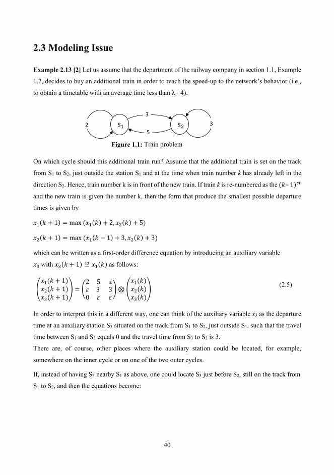
40

2.3 Modeling Issue

Example 2.13 [2] Let us assume that the department of the railway company in section 1.1, Example

1.2, decides to buy an additional train in order to reach the speed-up to the network’s behavior (i.e.,

to obtain a timetable with an average time less than λ =4).

Figure 1.1: Train problem

On which cycle should this additional train run? Assume that the additional train is set on the track

from S1 to S2, just outside the station S1 and at the time when train number k has already left in the

direction S2. Hence, train number k is in front of the new train. If train k is re-numbered as the (𝑘𝑘– 1)𝑠𝑠𝑡𝑡

and the new train is given the number k, then the form that produce the smallest possible departure

times is given by

𝑥𝑥1(𝑘𝑘 + 1) = max (𝑥𝑥1(𝑘𝑘) + 2, 𝑥𝑥2(𝑘𝑘) + 5)

𝑥𝑥2(𝑘𝑘 + 1) = max (𝑥𝑥1(𝑘𝑘 − 1) + 3, 𝑥𝑥2(𝑘𝑘) + 3)

which can be written as a first-order difference equation by introducing an auxiliary variable

𝑥𝑥3 with 𝑥𝑥3(𝑘𝑘 + 1) ≝ 𝑥𝑥1(𝑘𝑘) as follows:

𝑥𝑥1(𝑘𝑘 + 1)𝑥𝑥2(𝑘𝑘 + 1)𝑥𝑥3(𝑘𝑘 + 1)

= 2 5 𝜀𝜀𝜀𝜀 3 30 𝜀𝜀 𝜀𝜀

⊗ 𝑥𝑥1(𝑘𝑘)𝑥𝑥2(𝑘𝑘)𝑥𝑥3(𝑘𝑘)

(2.5)

In order to interpret this in a different way, one can think of the auxiliary variable x3 as the departure

time at an auxiliary station S3 situated on the track from S1 to S2, just outside S1, such that the travel

time between S1 and S3 equals 0 and the travel time from S3 to S2 is 3. There are, of course, other places where the auxiliary station could be located, for example,

somewhere on the inner cycle or on one of the two outer cycles.

If, instead of having S3 nearby S1 as above, one could locate S3 just before S2, still on the track from

S1 to S2, and then the equations become:

3 s1 s2

3

5

2

41

𝑥𝑥1(𝑘𝑘 + 1)𝑥𝑥2(𝑘𝑘 + 1)𝑥𝑥3(𝑘𝑘 + 1)

= 2 5 𝜀𝜀𝜀𝜀 3 03 𝜀𝜀 𝜀𝜀

⊗ 𝑥𝑥1(𝑘𝑘)𝑥𝑥2(𝑘𝑘)𝑥𝑥3(𝑘𝑘)

(2.6)

However, with S3 just after S2 on the track towards S1,

𝑥𝑥1(𝑘𝑘 + 1)𝑥𝑥2(𝑘𝑘 + 1)𝑥𝑥3(𝑘𝑘 + 1)

= 2 𝜀𝜀 53 3 𝜀𝜀𝜀𝜀 0 𝜀𝜀

⊗ 𝑥𝑥1(𝑘𝑘)𝑥𝑥2(𝑘𝑘)𝑥𝑥3(𝑘𝑘)

(2.7)

Each of the three models (2.5), (2.6), and (2.7) essentially describes the same speed-up of the

network’s behavior. It is not astonishing, then, that the eigenvalues of the three matrices are identical.

A little exercise shows that these eigenvalues all equal 3. That the eigenvalues cannot be smaller than

3 is easy to understand, since the outer cycle at S2 has one train and the travel time equals 3. On the

inner cycle, the average interdeparture time cannot be smaller than 8/3. Evidently, the outer cycle at

S2 has now become the predicament. A small calculation will provide that eigenvectors corresponding

to models (2.5), (2.6), and (2.7) will be

0

−2

−3

,

0

−2

0

and

0

1

−2

respectively. Since eigenvectors are determined up to the addition of a constant, the eigenvectors

given above are scaled in such a way that the first element is equal to zero. For the first (and second)

model, the departure times at S1 are 0,3,6,9, . . ., and for S2 they are −2,1,4,7, . . ..for the third model

these sequences are 0,3,6,9, . ..and 1,4,7,10, . . ., respectively.

Thus, one notices that the kth departure time at S2 of model (2.6) coincides with the (𝑘𝑘 – 1)𝑠𝑠𝑡𝑡

departure time at S2 of model (2.7).

Apparently, the geographical shift of station S3 on the inner cycle, from just before S2 to just after it,

causes a shift in the counting of the departures and their times.

42

2.4 Max-plus Linear Discrete Event Systems

2.4.1 Max-plus Linear State Space Models

A Discrete Event System (DES) only with synchronization and no concurrency can be modeled by a

max-plus-algebraic model as:

𝑥𝑥(𝑘𝑘) = 𝐴𝐴⨂𝑥𝑥(𝑘𝑘 − 1)⨁𝐵𝐵⨂𝑢𝑢(𝑘𝑘)

𝑦𝑦(𝑘𝑘) = 𝐶𝐶⨂𝑥𝑥(𝑘𝑘) (2.8)

with 𝐴𝐴 ∈ ℝmax𝑛𝑛×𝑛𝑛 ,𝐵𝐵 ∈ ℝmax

𝑛𝑛×𝑚𝑚, and 𝐶𝐶 ∈ ℝmax𝑙𝑙×𝑛𝑛 where m is the number of inputs and l the number of

outputs. The vector x represents the state, u is the input vector, and y is the output vector of the system.

It is important to note that in (2.8) the components of the input, the output, and the state are event

times, and that the counter k in (2.8) is an event counter. For a manufacturing system, u(k) would

typically represent the time instants at which raw material is fed to the system for the kth time, x(k)

the time instants at which the machines start processing the kth batch of intermediate products, and

y(k) the time instants at which the kth batch of finished products leaves the system. Due to the analogy

with conventional linear time-invariant systems, a DES that can be modeled by (2.8) will be called a

max-plus linear time-invariant DES system. Typical examples of systems that can be modeled as max-plus linear DES are production systems,

railway networks, urban traffic networks, and queuing systems.

We will now illustrate in detail how a max-plus linear model of the form (2.8) can describe the

behavior of a simple manufacturing system. Consider the production system of Figure 2.5 [3].

d1

t1 t3 d3

u(k) d2 t4 t5 y(k)

t2

Figure 2.5: A simple manufacturing system

This manufacturing system consists of three processing units: P1, P2 and P3, and works in batches

(one batch for each finished product). Raw material is fed to P1 and P2, processed and sent to P3,

P1

P2

P3

43

where assembly takes place. Note that each input batch of raw material is split into two parts: one

part of the batch goes to P1 and the other part goes to P2.

The processing times for P1, P2 and P3 are respectively d1, d2 and d3 time units. We assume that it

takes t1 time units for the raw material to get from the input source to P1, and t3 time units for a

finished product of P1 to get to P3. The other transportation times (t2, t4, and t5) are assumed

to be negligible.

At the input of the system and between the processing units, there are buffers with a capacity that is

large enough to ensure that no buffer overflow occurs. A processing unit can only start working on a

new product if it has finished processing the previous one. We assume that each processing unit starts

working as soon as all parts are available.

Now we write down the max-plus-algebraic state space model of this DES. First, we determine

𝑥𝑥1(𝑘𝑘), i.e., the time instant at which the processing unit P1 starts working for the kth time. If we feed

raw material to the system for the kth time, then this raw material is available at the input of the

processing unit P1 at time 𝑡𝑡 = 𝑢𝑢(𝑘𝑘) + 𝑡𝑡1.

However, P1 can only start working on the new batch of raw material as soon as it has finished

processing the current, i.e. the(𝑘𝑘 – 1)𝑡𝑡ℎ, batch.

Since the processing time on P1 is d1 time units, the (𝑘𝑘 – 1)𝑡𝑡ℎ intermediate product will leave P1 at

time 𝑡𝑡 = 𝑥𝑥1(𝑘𝑘 − 1) + 𝑑𝑑1.

Since P1 starts working on a batch of raw material as soon as the raw material is available and the

current batch has left the processing unit, this implies that we have

𝑥𝑥1(𝑘𝑘) = max (𝑥𝑥1(𝑘𝑘 − 1) + 𝑑𝑑1,𝑢𝑢(𝑘𝑘) + 𝑡𝑡1).

Using a similar reasoning, we find

𝑥𝑥2(𝑘𝑘) = max (𝑥𝑥2(𝑘𝑘 − 1) + 𝑑𝑑2,𝑢𝑢(𝑘𝑘) + 𝑡𝑡2)

𝑥𝑥3(𝑘𝑘) = max (𝑥𝑥1(𝑘𝑘) + 𝑑𝑑1 + 𝑡𝑡3, 𝑥𝑥2(𝑘𝑘) + 𝑑𝑑2 + 𝑡𝑡4, 𝑥𝑥3(𝑘𝑘 − 1) + 𝑑𝑑3,𝑢𝑢(𝑘𝑘) + max (𝑑𝑑1 + 𝑡𝑡1 + 𝑡𝑡3,𝑑𝑑2 +

𝑡𝑡2 + 𝑡𝑡4)

𝑦𝑦(𝑘𝑘) = 𝑥𝑥3(𝑘𝑘) + 𝑑𝑑3 + 𝑡𝑡5.

If we rewrite the above evolution equations as a max-plus-linear discrete event systems state space

model of the form (2.8), we obtain

𝑥𝑥(𝑘𝑘) =

𝑑𝑑1 𝜀𝜀 𝜀𝜀

𝜀𝜀 𝑑𝑑2 𝜀𝜀

2𝑑𝑑1 + 𝑡𝑡3 2𝑑𝑑2 + 𝑡𝑡4 𝑑𝑑3

⊗ 𝑥𝑥(𝑘𝑘 − 1) ⊕

𝑡𝑡1 𝑡𝑡2max(𝑑𝑑1 + 𝑡𝑡1 + 𝑡𝑡3,𝑑𝑑2 + 𝑡𝑡2 + 𝑡𝑡4)

⊗ 𝑢𝑢(𝑘𝑘)

𝑦𝑦(𝑘𝑘) = (𝜀𝜀 𝜀𝜀 𝑑𝑑3 + 𝑡𝑡5) ⊗𝑥𝑥(𝑘𝑘)

44

2.4.2 Example of Simple Production System

Example 2.14 Consider the simple production system of Figure 2.6. [3].

d1=5

t1=2 t3=1 d3=3

u(k) d2=6 t4=0 t5=0 y(k)

t2=0

Figure 2.5: A simple manufacturing system

This system consists of three processing units: P1, P2, and P3. Raw material is fed to P1 and P2,

processed, and sent to P3 where assembly takes place. The processing times for P1, P2, and P3 are

respectively d1 =5, d2 =6, and d3 =3 time units.

We assume that it takes t1 = 2 time units for the raw material to get from the input source to P1 and

that it takes t3 = 1 time unit for the finished products of processing unit P1 to reach P3.

The other transportation times (t2, t4, and t5) are assumed to be negligible. At the input of the system

and between the processing units, there are buffers with a capacity that is large enough to ensure that

no buffer overflow will occur. Initially all buffers are empty and none of the processing units contains

raw material or intermediate products.

A processing unit can only start working on a new product if it has finished processing the previous

one. We assume that each processing unit starts working as soon as all parts are available. Define

• 𝑢𝑢(𝑘𝑘): time instant at which raw material is fed to the system for the kth time,

• 𝑥𝑥𝑖𝑖(𝑘𝑘): time instant at which the ith processing unit starts working for the kth time,

• 𝑦𝑦 (𝑘𝑘): time instant at which the kth finished product leaves the system.

Let us now determine the time instant at which the processing unit P1 starts working for the kth time.

If we feed raw material to the system for the kth time, then this raw material is available at the input

of processing unit P1 at time 𝑡𝑡 = 𝑢𝑢(𝑘𝑘) + 2. However, P1 can only start working on the new batch of

raw material as soon as it has finished processing the previous, i.e., the (𝑘𝑘 – 1)𝑠𝑠𝑡𝑡, batch. Since the

processing time on P1 is d1 = 5 time units, the (𝑘𝑘 – 1)𝑠𝑠𝑡𝑡 intermediate product will leave P1 at time

𝑡𝑡 = 𝑥𝑥1(𝑘𝑘 − 1) + 5. Since P1 starts working on a batch of raw material as soon as the raw material is

available and the current batch has left the processing unit, this implies that we have

P1

P2

P3

45

𝑥𝑥1(𝑘𝑘) = max(𝑥𝑥1(𝑘𝑘 − 1) + 5,𝑢𝑢(𝑘𝑘) + 2) (2.9)

for k =1,2, . . . The condition that initially the processing unit P1 is empty and idle corresponds to the

initial condition x1(0)= ε since then it follows from (2.9) that 𝑥𝑥1(1) = 𝑢𝑢(1) + 2, i.e., the first batch

of raw material that is fed to the system will be processed immediately (after a delay of 2 time units

needed to transport the raw material from the input to P1).

Using a similar reasoning, we find the following expressions for the time instants at which P2 and P3

start working for the (𝑘𝑘 + 1)𝑠𝑠𝑡𝑡time and for the time instant at which the kth-finished product leaves

the system:

𝑥𝑥2(𝑘𝑘) = max(𝑥𝑥2(𝑘𝑘 − 1) + 6, 𝑢𝑢(𝑘𝑘) + 0) (2.10)

𝑥𝑥3(𝑘𝑘) = max(𝑥𝑥1(𝑘𝑘) + 5 + 1, 𝑥𝑥2(𝑘𝑘) + 6 + 0, 𝑥𝑥3(𝑘𝑘 − 1) + 3)

= max(𝑥𝑥1(𝑘𝑘 − 1) + 11, 𝑥𝑥2(𝑘𝑘 − 1) + 12, 𝑥𝑥3(𝑘𝑘 − 1) + 3,𝑢𝑢(𝑘𝑘) + 8)

(2.11)

𝑦𝑦(𝑘𝑘) = 𝑥𝑥3(𝑘𝑘) + 3 + 0 (2.12)

For 𝑘𝑘 = 1, 2 . .. The condition that initially all buffers are empty corresponds to the initial condition

𝑥𝑥1(0) = 𝑥𝑥2(0) = 𝑥𝑥3(0) = 𝜀𝜀.

Let us now rewrite the equations of the production system using the symbols ⨁ and ⨂; in that case,

(2.9) can be written as

𝑥𝑥1(𝑘𝑘) = 5 ⊗ 𝑥𝑥1(𝑘𝑘 − 1) ⊕ 2 ⊗ 𝑢𝑢(𝑘𝑘) .

If we do the same for (2.4) – (2.6), the resulting equations in max-plus-algebraic matrix notation, we

obtain

𝑥𝑥(𝑘𝑘) =

5 𝜀𝜀 𝜀𝜀

𝜀𝜀 6 𝜀𝜀

11 12 3

⊗ 𝑥𝑥(𝑘𝑘 − 1) ⊕

2

0

8

⊗ 𝑢𝑢(𝑘𝑘)

𝑦𝑦(𝑘𝑘) = [𝜀𝜀 𝜀𝜀 3] ⊗𝑥𝑥(𝑘𝑘),

where 𝑥𝑥(𝑘𝑘) = [𝑥𝑥1(𝑘𝑘) 𝑥𝑥2(𝑘𝑘) 𝑥𝑥3(𝑘𝑘)]𝑇𝑇 .

46

Example 2.15 Consider the more complex manufacturing system in Figure 2.7, which also can be

described by using the form (2.8). This manufacturing system consists of five processing units: P1,

P2, P3, P4 and P5 and works in batches (one batch for each finished product).

Figure 2.7: A manufacturing system

Raw material is fed to P1, P2 and P3. P1 and P2 are processed and sent to P4. P3 and P4 are processed

and sent to P5, where assembly takes place. Note that each input batch of raw material is split into

three parts: one part of the batch goes to P1, the second part goes to P2 and the third part goes to P3.

The processing times for P1, P2, P3 P4 and P5 are respectively d1, d2, d3, d4, d5 time units.

We assume that it takes t1 time units for the raw material to get from the input source to P1, and t4

time units for a finished product of P1 to get to P4, and t7 time units for a finished product of P4 to get

to P5. The other transportation times are assumed negligible.

At the input of the system and between the processing units, there are buffers with a capacity that is

large enough to ensure that no buffer overflow occurs. A processing unit can only start working on a

new product if it has finished processing the previous one. We assume that each processing unit starts

working as soon as all parts are available.

Now we write down the max-plus-algebraic state space model of this DES. First, we determine 𝑥𝑥1(𝑘𝑘),

i.e., the time instant at which processing unit P1 starts working for the kth time. If we feed raw material

to the system for the kth time, then this raw material is available at the input of processing unit P1 at

time 𝑡𝑡 = 𝑢𝑢(𝑘𝑘) + 𝑡𝑡1.

However, P1 can only start working on the new batch of raw material as soon as it has finished

processing the current, i.e. the (𝑘𝑘 − 1)𝑡𝑡ℎ, batch.

Since the processing time on P1 is d1 time units, the (𝑘𝑘 − 1)𝑡𝑡ℎ intermediate product will leave P1 at

time 𝑡𝑡 = 𝑥𝑥1(𝑘𝑘 − 1) + 𝑑𝑑1.

47

Since P1 starts working on a batch of raw material as soon as the raw material is available and the

current batch has left the processing unit, this implies that we have

𝑥𝑥1(𝑘𝑘) = max(𝑥𝑥1(𝑘𝑘 − 1) + 𝑑𝑑1,𝑢𝑢(𝑘𝑘) + 𝑡𝑡1)

Using a similar reasoning, we find

𝑥𝑥2(𝑘𝑘) = max(𝑥𝑥2(𝑘𝑘 − 1) + 𝑑𝑑2,𝑢𝑢(𝑘𝑘) + 𝑡𝑡2)

𝑥𝑥3(𝑘𝑘) = max(𝑥𝑥3(𝑘𝑘 − 1) + 𝑑𝑑3,𝑢𝑢(𝑘𝑘) + 𝑡𝑡3)

𝑥𝑥4(𝑘𝑘) = max(𝑥𝑥1(𝑘𝑘) + 𝑑𝑑1 + 𝑡𝑡4 , 𝑥𝑥2(𝑘𝑘) + 𝑑𝑑2 + 𝑡𝑡5, 𝑥𝑥4(𝑘𝑘 − 1) + 𝑑𝑑4 )

= max(𝑥𝑥1(𝑘𝑘 − 1) + 2𝑑𝑑1 + 𝑡𝑡4 , 𝑥𝑥2(𝑘𝑘 − 1) + 2𝑑𝑑2 + 𝑡𝑡5, 𝑥𝑥4(𝑘𝑘 − 1) + 𝑑𝑑4,𝑢𝑢(𝑘𝑘)

+ max(𝑑𝑑1 + 𝑡𝑡1 + 𝑡𝑡4 ,𝑑𝑑2 + 𝑡𝑡2 + 𝑡𝑡5))

𝑥𝑥5(𝑘𝑘) = max(𝑥𝑥3(𝑘𝑘) + 𝑑𝑑3 + 𝑡𝑡6 , 𝑥𝑥4(𝑘𝑘) + 𝑑𝑑4 + 𝑡𝑡7, 𝑥𝑥5(𝑘𝑘 − 1) + 𝑑𝑑5)

= max(𝑥𝑥3(𝑘𝑘 − 1) + 𝑑𝑑3 + 𝑑𝑑3 + 𝑡𝑡6,𝑢𝑢(𝑘𝑘) + 𝑡𝑡3 + 𝑑𝑑3 + 𝑡𝑡6, 𝑥𝑥1(𝑘𝑘 − 1) + 2𝑑𝑑1 + 𝑡𝑡4 + 𝑑𝑑4 +

𝑡𝑡7 , 𝑥𝑥2(𝑘𝑘 − 1) + 2𝑑𝑑2 + 𝑡𝑡5 + 𝑑𝑑4 + 𝑡𝑡7, 𝑥𝑥4(𝑘𝑘 − 1) + 𝑑𝑑4 + 𝑑𝑑4 + 𝑡𝑡7,𝑢𝑢(𝑘𝑘) +

max(𝑑𝑑1 + 𝑡𝑡1 + 𝑡𝑡4 + 𝑑𝑑4 + 𝑡𝑡7 ,𝑑𝑑2 + 𝑡𝑡2 + 𝑡𝑡5 + 𝑑𝑑4 + 𝑡𝑡7), 𝑥𝑥5(𝑘𝑘 − 1) + 𝑑𝑑5)

= max (𝑥𝑥1(𝑘𝑘 − 1) + 2𝑑𝑑1 + 𝑡𝑡4 + 𝑑𝑑4 + 𝑡𝑡7, 𝑥𝑥2(𝑘𝑘 − 1) + 2𝑑𝑑2 + 𝑡𝑡5 + 𝑑𝑑4 + 𝑡𝑡7, 𝑥𝑥3(𝑘𝑘 − 1) + 2𝑑𝑑3

+𝑡𝑡6 , 𝑥𝑥4(𝑘𝑘 − 1) + 2𝑑𝑑4 + 𝑡𝑡7, 𝑥𝑥5(𝑘𝑘 − 1) + 𝑑𝑑5 ,𝑢𝑢(𝑘𝑘) + max(𝑑𝑑3 + 𝑡𝑡6 + 𝑡𝑡3 ,𝑑𝑑1 + 𝑡𝑡1 + 𝑡𝑡4+ 𝑑𝑑4 + 𝑡𝑡7,𝑑𝑑2 + 𝑡𝑡2 + 𝑡𝑡5 + 𝑑𝑑4 + 𝑡𝑡7))

𝑦𝑦(𝑘𝑘) = 𝑥𝑥5(𝑘𝑘) + 𝑑𝑑5 + 𝑡𝑡8

If we rewrite the above equations as a Max-plus-linear discrete event systems state space model of

the form (2.8), we obtain

𝑥𝑥(𝑘𝑘) =

⎝

⎜⎜⎜⎛

𝑑𝑑1 𝜀𝜀 𝜀𝜀 𝜀𝜀 𝜀𝜀

𝜀𝜀 𝑑𝑑2 𝜀𝜀 𝜀𝜀 𝜀𝜀

𝜀𝜀 𝜀𝜀 𝑑𝑑3 𝜀𝜀 𝜀𝜀

2𝑑𝑑1 + 𝑡𝑡4 2𝑑𝑑2 + 𝑡𝑡5 𝜀𝜀 𝑑𝑑4 𝜀𝜀

2𝑑𝑑1 + 𝑡𝑡4 + 𝑑𝑑4 + 𝑡𝑡7 2𝑑𝑑2 + 𝑡𝑡5 + 𝑑𝑑4 + 𝑡𝑡7 2𝑑𝑑3 + 𝑡𝑡6 2𝑑𝑑4 + 𝑡𝑡7 𝑑𝑑5⎠

⎟⎟⎟⎞

⊗𝑥𝑥(𝑘𝑘 − 1) ⊕

⎝

⎜⎜⎜⎛

𝑡𝑡1 𝑡𝑡2 𝑡𝑡3max(𝑑𝑑1 + 𝑡𝑡1 + 𝑡𝑡4,𝑑𝑑2 + 𝑡𝑡2 + 𝑡𝑡5)

max(𝑑𝑑3 + 𝑡𝑡3 + 𝑡𝑡6, 𝑡𝑡1 + 𝑑𝑑1 + 𝑑𝑑4 + 𝑡𝑡4 + 𝑡𝑡7, 𝑡𝑡2 + 𝑑𝑑2 + 𝑡𝑡5 + 𝑑𝑑4 + 𝑡𝑡7)⎠

⎟⎟⎟⎞

⊗ 𝑢𝑢(𝑘𝑘)

48

𝑦𝑦(𝑘𝑘) = (𝜀𝜀 𝜀𝜀 𝜀𝜀 𝜀𝜀 𝑑𝑑5 + 𝑡𝑡8)⨂𝑥𝑥(𝑘𝑘),

where 𝑥𝑥(𝑘𝑘) = (𝑥𝑥1(𝑘𝑘) 𝑥𝑥2(𝑘𝑘) 𝑥𝑥3(𝑘𝑘) 𝑥𝑥4(𝑘𝑘) 𝑥𝑥5(𝑘𝑘))𝑇𝑇

2.5 An Introduction to Max-plus Algebraic System Theory In this section, we will introduce the system theory for max-plus linear time for DESs [3, 10]. In

Section 2.4, we have shown by some simple examples that time deterministic DESs in which the

sequence of the events and the duration of the activities are fixed or can be determined in advance

can be described by an 𝑛𝑛𝑡𝑡ℎ order state space model of the form

𝑥𝑥(𝑘𝑘) = 𝐴𝐴⨂𝑥𝑥(𝑘𝑘 − 1)⨁𝐵𝐵⨂𝑢𝑢(𝑘𝑘)

𝑦𝑦(𝑘𝑘) = 𝐶𝐶⨂𝑥𝑥(𝑘𝑘) (2.8)

For all 𝑘𝑘 ∈ 𝑁𝑁0 with an intial condition 𝑥𝑥(0) = 𝑥𝑥0 and where 𝐴𝐴 ∈ ℝmax𝑛𝑛×𝑛𝑛, 𝐵𝐵 ∈ ℝmax

𝑛𝑛×𝑚𝑚 and 𝐶𝐶 ∈ ℝmax𝑙𝑙×𝑛𝑛 .

Let us introduce some analysis techniques for DESs that can be described by a model of the form

(2.8).

𝑥𝑥(1) = 𝐴𝐴⨂𝑥𝑥(0)⨁𝐵𝐵⨂𝑢𝑢(0)

𝑥𝑥(2) = 𝐴𝐴⨂𝑥𝑥(1)⨁𝐵𝐵⨂𝑢𝑢(1)

= 𝐴𝐴⨂2⨂𝑥𝑥(0)⨁𝐴𝐴⨂𝐵𝐵⨂𝑢𝑢(0))⨁𝐵𝐵⨂𝑢𝑢(1)

Thus, 𝑥𝑥(𝑘𝑘) = 𝐴𝐴⨂𝑘𝑘⨂𝑥𝑥(0) ⊕𝑖𝑖=0𝑘𝑘−1 𝐴𝐴⨂(𝑘𝑘−𝑖𝑖−1)⨂𝐵𝐵⨂𝑢𝑢(𝑖𝑖)

where the empty max-algebraic sum ⊕𝑖𝑖=0𝑘𝑘−1 is equal to 𝜀𝜀𝑛𝑛×1 by definition.

𝑦𝑦(𝑘𝑘) = 𝐶𝐶 ⊗ 𝐴𝐴⊗𝑘𝑘 ⊗ 𝑥𝑥(0) ⊕⊗ 𝐶𝐶𝑘𝑘−1𝑖𝑖=0 ⊗ 𝐴𝐴𝑘𝑘−𝑖𝑖−1 ⊗ 𝐵𝐵⊗ 𝑢𝑢(𝑖𝑖) (2.13)

Consider two input sequences 𝑢𝑢1 = 𝑢𝑢1(𝑘𝑘)𝑘𝑘=0∞ , 𝑢𝑢2 = 𝑢𝑢2(𝑘𝑘)𝑘𝑘=0∞ .

Let 𝑦𝑦1 = 𝑦𝑦1(𝑘𝑘)𝑘𝑘=1∞ be the output sequence that corresponds to the input sequence (with initial

condition 𝑥𝑥1,0) and let 𝑦𝑦2 = 𝑦𝑦2(𝑘𝑘)𝑘𝑘=1∞ be the output sequence that corresponds to the input

sequence u2 (with initial condition 𝑥𝑥2,0).

Let 𝛼𝛼,𝛽𝛽 ∈ ℝmax. From (2.13) it follows that the output sequence that corresponds to the input

sequence 𝛼𝛼 ⊗ 𝑢𝑢1 ⊕ 𝛽𝛽⊗ 𝑢𝑢2 = 𝛼𝛼 ⊗ 𝑢𝑢1(𝑘𝑘)𝑘𝑘=0∞ ⊕𝛽𝛽⊗ 𝑢𝑢2(𝑘𝑘)𝑘𝑘=0∞ (with the initial condition

𝛼𝛼⨂𝑥𝑥1,0⨁𝛽𝛽⨂𝑥𝑥2,0) is given by 𝛼𝛼⨂𝑦𝑦1⨁𝛽𝛽⨂𝑦𝑦2.

This explains why DESs that can be described by a model of the form (2.8) are called max-linear.

Now we assume that 𝑥𝑥(0) = 𝜀𝜀𝑛𝑛×1 and let 𝑝𝑝 ∈ 𝑁𝑁0

49

If we define 𝑌𝑌 = 𝑦𝑦(1) 𝑦𝑦(2) … … 𝑦𝑦(𝑝𝑝)𝑇𝑇

and 𝑈𝑈 = (𝑢𝑢(0) 𝑢𝑢(1) … …𝑢𝑢(𝑝𝑝 − 1))𝑇𝑇,

then (2,13) results in 𝑌𝑌 = 𝐻𝐻⨂𝑈𝑈

𝐻𝐻 =

⎝

⎜⎜⎛

𝐶𝐶 ⊗𝐵𝐵 𝜀𝜀 … 𝜀𝜀

𝐶𝐶 ⊗ 𝐴𝐴⊗𝐵𝐵 𝐶𝐶 ⊗ 𝐵𝐵 … 𝜀𝜀

⋮ ⋮ ⋮

𝐶𝐶 ⊗ 𝐴𝐴⊗𝑡𝑡−1 ⊗ 𝐵𝐵 𝐶𝐶 ⊗ 𝐴𝐴⊗𝑡𝑡−2 ⊗ 𝐵𝐵 … 𝐶𝐶 ⊗𝐵𝐵 ⎠

⎟⎟⎞

For the production system of Example 2.14, Section 2.4, this means that if we know the time instants

at which raw material is fed to the system, we can compute the time instants at which the finished

products will leave the system.

If we know the vector Y of latest times at which the finished products have to leave the system, we

can compute the vector U of (latest) time instants at which raw material has to be fed to the system

by solving the system of max-plus linear equations 𝐻𝐻⨂𝑈𝑈 = 𝑌𝑌, if it has a solution, or finding the

greatest sub solution of 𝐻𝐻⨂𝑈𝑈 = 𝑌𝑌.

However, if we have perishable goods it is better to minimize the maximal deviation between the

required and the actual finishing times. In this case, we must solve the following problem:

minimize max𝑖𝑖

|(𝑌𝑌 − 𝐻𝐻⊗𝑈𝑈)𝑖𝑖|

This problem can be solved using Theorem 2.1. Let 𝑖𝑖 ∈ 1,2, … ,𝑚𝑚, a max-algebraic unit impulse is a

sequence that is defined as follows

𝑒𝑒(𝑘𝑘) = 0 if 𝑘𝑘 = 0

𝜀𝜀 if 𝑘𝑘 ≠ 0, for 𝑘𝑘 = 0, 1, 2, …

If we apply a max-plus algebra unit impulse to the 𝑖𝑖𝑡𝑡ℎ input of the system and if we suppose that

𝑥𝑥(0) = 𝜀𝜀𝑛𝑛×1 then we obtain

𝑦𝑦(𝑘𝑘) = 𝐶𝐶⨂𝐴𝐴⊗𝑘𝑘−1 ⊗ 𝐵𝐵𝑖𝑖, for 𝑘𝑘 = 1, 2, 3, …

as an output of the DES. This output is called the impulse response due to a max-plus algebraic

impulse at the 𝑖𝑖𝑡𝑡ℎ input. Note that 𝑦𝑦(𝑘𝑘) corresponds to the 𝑖𝑖𝑡𝑡ℎ column of the matrix,

𝐺𝐺𝑘𝑘−1 ≝ 𝐶𝐶⨂𝐴𝐴⊗𝑘𝑘−1 ⊗ 𝐵𝐵, for 𝑘𝑘 = 1, 2, 3, …

Therefore, the sequence 𝐺𝐺𝑘𝑘𝑘𝑘=0∞ is called the impulse response of the DES. The Gk's are called the

impulse response matrices or Markov parameters.

Example 2.14 section 2.4 shows the meaning to the impulse response of the production system. In

the beginning all the buffers of the system are empty, then begin to feed the raw materials in the

50

buffer input and continue to feed the raw materials at such a rate that the input buffer is never empty.

Moments in time that the final products leave the system are in accordance with the terms of the

impulse response.

Consider the autonomous DES described by

𝑥𝑥(𝑘𝑘 + 1) = 𝐴𝐴 ⊗ 𝑥𝑥(𝑘𝑘)

𝑦𝑦(𝑘𝑘) = 𝐶𝐶 ⊗ 𝑥𝑥(𝑘𝑘)

With 𝑥𝑥(0) = 𝑥𝑥0. For the production system of Example 2.14, section 2.4, this means that we start

from a situation in which some internal buffers and the entire input buffer are not empty in the

beginning, if 𝑥𝑥0 ≠ 𝜀𝜀𝑛𝑛×1, and that afterwards the raw material is fed to the system at such a rate that

the input buffers never become empty.

If the system matrix A is irreducible, then we can calculate the ultimate behavior of the autonomous

DES by solving the max-algebraic eigenvalue problem

𝐴𝐴⨂𝑣𝑣 = 𝜆𝜆 ⊗ 𝑣𝑣 there exist integers 𝑘𝑘0 ∈ 𝑁𝑁, 𝑐𝑐 ∈ 𝑁𝑁 such that

𝑥𝑥(𝑘𝑘 + 𝑐𝑐) = 𝜆𝜆⨂𝑐𝑐 ⊗ 𝑥𝑥(𝑘𝑘) which means

𝑥𝑥𝑖𝑖(𝑘𝑘 + 𝑐𝑐) − 𝑥𝑥𝑖𝑖(𝑘𝑘) = 𝑐𝑐𝜆𝜆 for 𝑖𝑖 = 1,2, … … , 𝑛𝑛 for all 𝑘𝑘 ≥ 𝑘𝑘0. (2.14)

This behavior will be called cyclic. From (2.14) it follows that for a production system 𝜆𝜆 will be the

average duration of a cycle of the production process when the system has reached its cyclic behavior.

The average production rate will then be equal 1𝜆𝜆.

Example 2.16 [3] Consider the production system of Example 2.14.

Define 𝑌𝑌 = [ 𝑦𝑦(1) 𝑦𝑦(2) 𝑦𝑦(3) 𝑦𝑦(4)]𝑇𝑇 and 𝑈𝑈 = [𝑢𝑢(0) 𝑢𝑢(1) 𝑢𝑢(2) 𝑢𝑢(3)]𝑇𝑇.

If 𝑥𝑥0 = 𝜀𝜀3×1, then we have 𝑌𝑌 = 𝐻𝐻⊗𝑈𝑈 with

𝐻𝐻 =

⎝

⎜⎛

11 𝜀𝜀 𝜀𝜀 𝜀𝜀

16 11 𝜀𝜀 𝜀𝜀

21 16 11 𝜀𝜀

27 21 16 11⎠

⎟⎞

If we feed raw material to the system at time instants 𝑢𝑢(0) = 0,𝑢𝑢(1) = 9,𝑢𝑢(2) = 12, 𝑢𝑢(3) = 15,

⇒ 𝑈𝑈 = 09

1215

51

⇒ 𝐻𝐻⨂𝑈𝑈 =

⎝

⎜⎛

11 𝜀𝜀 𝜀𝜀 𝜀𝜀

16 11 𝜀𝜀 𝜀𝜀

21 16 11 𝜀𝜀

27 21 16 11⎠

⎟⎞⨂

⎝

⎜⎛

0

9

12

15⎠

⎟⎞

=

⎝

⎜⎛

11

20

25

30⎠

⎟⎞

= 𝑌𝑌

Thus, the finished products will leave the system at time instants 𝑦𝑦(1) = 11,𝑦𝑦(2) = 20,𝑦𝑦(3) = 25

and 𝑦𝑦(4) = 30.

If the finished parts should leave the system before time instants 17, 19, 24 and 27 and if we want to

feed the raw material to the system as late as possible, then we should feed raw material to the system

at time instants 0, 6, 11, 16, since [0 6 11 16]𝑇𝑇 is the greatest subsolution of

𝐻𝐻⊗ 𝑈𝑈 =

⎝

⎜⎛

17

19

24

27⎠

⎟⎞

The impulse response of the system is given by

𝐺𝐺𝑘𝑘𝑘𝑘=0∞ = 11, 16, 21, 27, 33, 39, 45, 51, 57, 63, 69, 75, … … …

Although the system matrix A is not irreducible, the system in the autonomous case does exhibit an

ultimately cyclic behavior of the form (2.14) with 𝜆𝜆 = 6 and 𝑐𝑐 = 1 . It is easy to verify that 𝜆𝜆

corresponds to the largest average cycle weight of the precedence graph of 𝐴𝐴 (See Figure 2.8) and to

the largest max-algebraic eigenvalue of A. If we feed the system by raw material at a rate such that

the input buffer never becomes empty, then after a finite number of production cycles, the difference

between 𝑥𝑥𝑖𝑖(𝑘𝑘 + 1) and 𝑥𝑥𝑖𝑖(𝑘𝑘) will be equal to 6 for all processing units Pi.

Thus, the average production rate of the system is 16, i.e. every 6 time units a finished part leaves the

production system.

5 6

11 12

3

Figure 2.8: The precedence graph of the matrix A of example 2.13 section 2.4

1 2

3

52

2.6 Characteristic Equation and the Cayley-Hamilton

Theorem

This section is organized as follows: In 2.6.1, we introduce some notations and definitions. In

Subsection 2.6.2, we give a short introduction to the characteristic equation and the Cayley-Hamilton

theorem in conventional algebra [1, 7]. In 2.6.3, we derive the characteristic equation of a matrix in

the max-plus algebra. We also include an example in which we compute the max-algebraic

characteristic equation of a given matrix [1], [7] and [11].

2.6.1 Notations and Definitions If A is a set, then |𝐴𝐴| denotes the number of elements of A. We use 𝑃𝑃𝑛𝑛 to represent the set of all

permutations of n numbers. The set of even permutations of 𝑛𝑛 numbers is denoted by 𝑃𝑃𝑛𝑛𝑒𝑒. and the set

of the odd permutations of 𝑛𝑛 numbers is denoted by 𝑃𝑃𝑛𝑛0. An element σ of 𝑃𝑃𝑛𝑛 will be considered as a

mapping from 1, 2, . . . ,𝑛𝑛 to 1, 2, . . . ,𝑛𝑛.

We say a permutation is even if it can be written as a product of an even number of (usually non-

disjoint) transpositions (i.e. 2-cycles). Likewise, a permutation is odd if it can be written as a product

of an odd number of transpositions [7].

Let Sn be the symmetric group associated to the bijections of the set = 1,2, … , 𝑛𝑛. A transposition is

a 2-cycle 𝑐𝑐 𝑘𝑘 𝑆𝑆𝑛𝑛. It is known that transpositions generate Sn. Equivalently stated, every permutation

can be written as a product of transpositions. Notice, though, that unlike the decomposition of σ into

disjoint cycles, the decomposition of a permutation as a product of transpositions is not unique!

However, the parity of the number of transpositions which appear in any such decomposition is

independent from the chosen decomposition. Let 𝑠𝑠 be the number of transpositions which appear in

a decomposition of 𝜎𝜎𝑘𝑘 𝑆𝑆𝑛𝑛.

Definition 2.3 The signature of σ is

sgn(𝜎𝜎) = (−1)𝑠𝑠.

There is an equivalent way to state the definition of the signature of a permutation σ by considering

the canonical decomposition of σ into disjoint cycles.

Let us assume that the decomposition of σ into disjoint cycles is given by 𝜎𝜎 = 𝑐𝑐1 … 𝑐𝑐𝑟𝑟.

53

Definition 2.4 The signature of a r-cycle 𝑐𝑐 ∈ 𝑆𝑆𝑛𝑛 is

sgn(𝑐𝑐) = −1 if 𝑟𝑟 is odd

1 if 𝑟𝑟 is even

Consequently, we set

Definition 2.5 The signature of the permutation 𝜎𝜎 = 𝑐𝑐1 … … 𝑐𝑐𝑟𝑟 is

sgn( 𝑐𝑐) = ∏ sgn( 𝑐𝑐𝑖𝑖).𝑟𝑟𝑖𝑖=1

The signature of the permutation σ is denoted by sgn(σ). We use 𝐶𝐶𝑘𝑘𝑛𝑛 to represent the set of all subsets

with k elements of the set 1, 2, . . . ,𝑛𝑛.

Let 𝐴𝐴 be an n by n matrix and let 𝜙𝜙 ⊆ 1, 2, . . . ,𝑛𝑛. The submatrix obtained by removing all rows

and columns of 𝐴𝐴 except for those indexed by ϕ is denoted by 𝐴𝐴𝜑𝜑𝜑𝜑 . The matrix 𝐴𝐴𝜑𝜑𝜑𝜑 is called a

principal submatrix of the matrix 𝐴𝐴.

Definition 2.6 Let f and g be real functions. The function f is asymptotically equivalent to g in the

neighborhood of ∞, denoted by 𝑓𝑓(𝑥𝑥) ∼ 𝑔𝑔(𝑥𝑥), 𝑥𝑥 → ∞,

if lim𝑚𝑚→∞

𝑓𝑓(𝑚𝑚)𝑔𝑔(𝑚𝑚)

= 1.

We say that 𝑓𝑓(𝑥𝑥) ≈ 0, 𝑥𝑥 → ∞ if there is a real number K such that

𝑓𝑓(𝑥𝑥) = 0 for all 𝑥𝑥 ≥ 𝐾𝐾.

If F and G are real m by n matrix-valued functions, then we have 𝐹𝐹(𝑥𝑥) ∼ 𝐺𝐺(𝑥𝑥) when

𝒙𝒙 → ∞ if 𝑓𝑓𝑖𝑖𝑖𝑖(𝑥𝑥) ∼ 𝑔𝑔𝑖𝑖𝑖𝑖(𝑥𝑥) when 𝑥𝑥 → ∞ for all 𝑖𝑖, 𝑗𝑗.

2.6.2 The Characteristic Equation in Ordinary Linear Algebra

In conventional linear algebra, the Cayley–Hamilton theorem (named after the mathematicians

Arthur Cayley and William Hamilton) states that every square matrix over a commutative ring

(including the real or complex field) satisfies its own characteristic equation [1], [7] and [11].

More specifically, if A is a given 𝑛𝑛 × 𝑛𝑛 matrix and 𝐼𝐼𝑛𝑛 is the 𝑛𝑛 × 𝑛𝑛 identity matrix, then the

characteristic polynomial of A is defined as:

𝑝𝑝(𝜆𝜆) = det(𝜆𝜆𝐼𝐼𝑛𝑛 − 𝐴𝐴)

where "det" is the determinant operation, since the entries of the matrix are (linear or constant)

polynomials in 𝜆𝜆, the determinant is also a polynomial in 𝜆𝜆.

54

The Cayley–Hamilton theorem declares that ″substituting″ the matrix 𝐴𝐴 for 𝜆𝜆 in these polynomial

results in zero matrices: P(A) = 0.

The powers of λ that have become powers of A by the substitution should be computed by repeated

matrix multiplication, and the constant term should be multiplied by the identity matrix (the zeroth

power of A) so that it can be added to the other terms.

The Cayley–Hamilton theorem is equivalent to the statement that the minimal polynomial of a square

matrix divides its characteristic polynomial.

Example 2.17 As a concrete example [7].

Let 𝐴𝐴 = 1 23 4 its characteristic polynomial given by

𝑝𝑝(𝜆𝜆) = det(𝜆𝜆 × 𝐼𝐼2 − 𝐴𝐴) = 𝜆𝜆 − 1 −2

−3 𝜆𝜆 − 4

= (𝜆𝜆 − 1)(𝜆𝜆 − 4) − (−2)(−3) = 𝜆𝜆2 − 5𝜆𝜆 − 2.

The Cayley–Hamilton theorem claims that if we define

𝑝𝑝(𝑋𝑋) = 𝑋𝑋 2 − 5𝑋𝑋 − 2𝐼𝐼2 , then

𝑝𝑝(𝐴𝐴) = 𝐴𝐴 2 − 5𝐴𝐴 − 2𝐼𝐼2 = 0 0

0 0

which one can easily verify.

Note: The characteristic equation in conventional algebra is used to calculate the eigenvalue of a

matrix.

Now we need to define a characteristic polynomial, characteristic equation and provide an analogue

of the Cayley–Hamilton theorem in max-plus algebra.

2.6.3 The Characteristic Equation in Max-plus Algebra

To derive the max-plus algebraic characteristic equation of a matrix [1],

let 𝑎𝑎, 𝑏𝑏, 𝑐𝑐 ∈ ℝmax then we have:

𝑎𝑎⨁𝑏𝑏 = 𝑐𝑐 ⇔ 𝑧𝑧𝑚𝑚 + 𝑧𝑧𝑏𝑏 ≃ 𝛼𝛼𝑧𝑧𝑐𝑐 when 𝑧𝑧 → ∞

𝑎𝑎⨂𝑏𝑏 = 𝑐𝑐 ⇔ 𝑧𝑧𝑚𝑚𝑧𝑧𝑏𝑏 = 𝑧𝑧𝑐𝑐 for all 𝑧𝑧 ∈ ℝ+

where 𝛼𝛼 = 1 if 𝑎𝑎 ≠ 𝑏𝑏 and 𝛼𝛼 = 2 if 𝑎𝑎 = 𝑏𝑏 and where 𝑧𝑧𝜀𝜀 = 0 for all 𝑧𝑧 ∈ ℝ+ by definition.

If 𝐴𝐴 ∈ ℝmax𝑛𝑛×𝑛𝑛 then zA is a real n by n matrix with domain of definition ℝ+ that is defined by

55

(𝑧𝑧𝐴𝐴)𝑖𝑖𝑖𝑖 = 𝑧𝑧𝑚𝑚𝑖𝑖𝑗𝑗for all 𝑖𝑖, 𝑗𝑗.

The dominant of A is defined as follows:

dom⊕𝐴𝐴 = the highest exponent in det 𝑧𝑧𝐴𝐴 if det 𝑧𝑧𝐴𝐴 ≠ 0,

𝜀𝜀 otherwise.

Theorem 2.5: Suppose that 𝐴𝐴 ∈ ℝmax𝑛𝑛×𝑛𝑛, if

det(𝜆𝜆𝐼𝐼𝑛𝑛 − 𝑧𝑧A) = 𝜆𝜆𝑛𝑛 + 𝑐𝑐1𝜆𝜆𝑛𝑛−1 + 𝑐𝑐2𝜆𝜆𝑛𝑛−2 + ⋯+ 𝑐𝑐𝑛𝑛−1𝜆𝜆 + 𝑐𝑐𝑛𝑛 then

𝐴𝐴𝑛𝑛 + 𝑐𝑐1𝐴𝐴𝑛𝑛−1 + 𝑐𝑐2𝐴𝐴𝑛𝑛−2 + ⋯+ 𝑐𝑐𝑛𝑛−1𝐴𝐴 + 𝑐𝑐𝑛𝑛𝐼𝐼 = 0

where 𝑐𝑐𝑘𝑘 = (−1)𝑘𝑘 ∑ det𝐴𝐴𝜑𝜑𝜑𝜑𝜑𝜑∈𝐶𝐶𝑛𝑛𝑘𝑘

We will show how the Cayley–Hamilton Theorem can be translated into max-plus algebra. We

consider the matrix 𝑧𝑧𝐴𝐴 [1], [7]. We also need a few more definitions.

First, we have the characteristic polynomial of the matrix valued function 𝑧𝑧𝐴𝐴 given by:

det( 𝜆𝜆𝐼𝐼 − 𝑧𝑧𝐴𝐴) = 𝜆𝜆𝑛𝑛 + 𝛾𝛾1(𝑧𝑧) 𝜆𝜆𝑛𝑛−1+. . . . . . +𝛾𝛾𝑛𝑛−1(𝑧𝑧) 𝜆𝜆 + 𝛾𝛾𝑛𝑛(𝑧𝑧) (2.15)

With coefficients:

𝛾𝛾𝑘𝑘(𝑧𝑧) = (−1)𝑘𝑘 ∑ det 𝑧𝑧𝐴𝐴𝜙𝜙𝜙𝜙𝜙𝜙∈𝐶𝐶𝑛𝑛𝑘𝑘 (2.16)

Therefore

(𝑧𝑧𝐴𝐴)𝑛𝑛 + 𝛾𝛾1(𝑧𝑧)(𝑧𝑧𝐴𝐴)𝑛𝑛−1+. . . . +𝛾𝛾𝑛𝑛−1(𝑧𝑧)𝑧𝑧𝐴𝐴 + 𝛾𝛾𝑛𝑛𝐼𝐼𝑛𝑛 = 0 (2.17)

For all 𝑧𝑧 ∈ ℝ+.

This is just the result of applying Theorem 2.5 to the matrix 𝑧𝑧𝐴𝐴.

The highest degree in (2.16) is equal to max𝑑𝑑𝑑𝑑𝑚𝑚⊕𝐴𝐴𝜙𝜙𝜙𝜙|𝜙𝜙 ∈ 𝐶𝐶𝑛𝑛𝑘𝑘 and

𝛾𝛾𝑘𝑘(𝑧𝑧)~(−1)𝑘𝑘 𝛾𝛾𝑘𝑘 𝑧𝑧max𝑑𝑑𝑜𝑜𝑚𝑚⊕𝐴𝐴𝜙𝜙𝜙𝜙𝜙𝜙∈𝐶𝐶𝑛𝑛𝑘𝑘 , 𝑧𝑧 → ∞

where 𝛾𝑘𝑘 is equal to the number of permutations that contribute to the highest degree in (2.15) taking

away the 𝑃𝑃𝑛𝑛𝑜𝑜. However, the highest degree in (2.15) is not necessarily equal to

max𝑑𝑑𝑑𝑑𝑚𝑚⊕𝐴𝐴𝜙𝜙𝜙𝜙|𝜙𝜙 ∈ 𝐶𝐶𝑛𝑛𝑘𝑘 since if 𝑃𝑃𝑛𝑛𝑒𝑒 that contribute to 𝑧𝑧max𝑑𝑑𝑜𝑜𝑚𝑚⊕𝐴𝐴𝜙𝜙𝜙𝜙𝜙𝜙∈𝐶𝐶𝑛𝑛𝑘𝑘 is equal to 𝑃𝑃𝑛𝑛𝑜𝑜 that

contribute to 𝑧𝑧max𝑑𝑑𝑜𝑜𝑚𝑚⊕𝐴𝐴𝜙𝜙𝜙𝜙𝜙𝜙∈𝐶𝐶𝑛𝑛𝑘𝑘 the term that contains 𝑧𝑧max𝑑𝑑𝑜𝑜𝑚𝑚⊕𝐴𝐴𝜙𝜙𝜙𝜙𝜙𝜙∈𝐶𝐶𝑛𝑛𝑘𝑘 disappears.

Note: Recall that 𝑃𝑃𝑛𝑛 represents the set of all permutations of 𝑛𝑛 number 𝜎𝜎: 1,2, … ,𝑛𝑛 → 1,2, … ,𝑛𝑛.

The set of the even permutations of 𝑛𝑛 numbers is denoted by 𝑃𝑃𝑛𝑛𝑒𝑒 and the set of the odd permutations

of 𝑛𝑛 numbers is denoted by 𝑃𝑃𝑛𝑛𝑜𝑜.

56

Example 2.18 Consider the matrix A [7], where

𝐴𝐴 =

−1 ε 2

0 2 ε

1 0 1

so the matrix valued function z𝐴𝐴 = 𝑧𝑧−1 0 z2

1 z2 0

z 0 z

so det 𝑧𝑧𝐴𝐴1,2,1,2 = det𝑧𝑧−1 0

1 z2 = 𝑧𝑧

det 𝑧𝑧 𝐴𝐴1,3,1,3 = det𝑧𝑧−1 z2

z z = −𝑧𝑧3 + 1

det 𝑧𝑧𝐴𝐴2,3,2,3 = det 𝑧𝑧2 0

0 z = 𝑧𝑧3

⇒ dom⊕𝐴𝐴1,2,1,2 = 1, dom⊕𝐴𝐴1,3,1,3 = 3 and dom⊕𝐴𝐴2,3,2,3 = 3

and because γ𝑘𝑘(𝑧𝑧) = (−1)𝑘𝑘 ∑ det z𝐴𝐴𝜑𝜑𝜑𝜑𝜙𝜙∈𝑐𝑐𝑛𝑛𝑘𝑘

⇒ 𝛾𝛾2(𝑧𝑧) = (−1)2(det z𝐴𝐴1,2,1,2 + det z𝐴𝐴1,3,1,3 + det z𝐴𝐴2,3,2,3)

= 𝑧𝑧 − 𝑧𝑧3 + 𝑧𝑧3 + 1

= z+1

Hence, the highest degree of the polynomial 𝛾𝛾2(𝑧𝑧) is equal to 1 but

max dom⊕𝐴𝐴𝜙𝜙𝜙𝜙 | 𝜙𝜙 ∈ 𝐶𝐶32 = 3 ≠ 1.

The highest degree term in (2.16) can be determined as follows:

Let us define Γ𝑘𝑘 = 𝜁𝜁:∃𝑖𝑖1, 𝑖𝑖2, . . . , 𝑖𝑖𝑘𝑘 ∈ 𝐶𝐶𝑛𝑛𝑘𝑘 ,∃ 𝜎𝜎 ∈ 𝑃𝑃𝑘𝑘 such that ζ = 𝑎𝑎 𝑖𝑖𝑟𝑟𝑖𝑖𝜎𝜎(𝑟𝑟)

𝑘𝑘

𝑟𝑟=1

for

𝑘𝑘 = 1,2, . . . ,𝑛𝑛. For every 𝑘𝑘 ∈ 1,2, . . . ,𝑛𝑛 and for every 𝜁𝜁 ∈ Γ𝑘𝑘 we can define:

𝐼𝐼𝑘𝑘𝑒𝑒(𝜁𝜁) = 𝜎𝜎 ∈ 𝑃𝑃𝑘𝑘𝑒𝑒 | ∃𝑖𝑖1, 𝑖𝑖2, . . . . , 𝑖𝑖𝑘𝑘 ∈ 𝐶𝐶𝑛𝑛𝑘𝑘 , such that 𝑎𝑎𝑖𝑖𝑟𝑟𝑖𝑖𝜎𝜎(𝑟𝑟) = 𝜁𝜁𝑘𝑘

𝑟𝑟=1

𝐼𝐼𝑘𝑘𝑜𝑜(𝜁𝜁) = 𝜎𝜎 ∈ 𝑃𝑃𝑘𝑘𝑜𝑜 | ∃𝑖𝑖1, 𝑖𝑖2, . . . . , 𝑖𝑖𝑘𝑘 ∈ 𝐶𝐶𝑛𝑛𝑘𝑘, such that 𝑎𝑎𝑖𝑖𝑟𝑟𝑖𝑖𝜎𝜎(𝑟𝑟)

𝑘𝑘

𝑟𝑟=1

= 𝜁𝜁

𝐼𝐼𝑘𝑘(𝜁𝜁) = 𝐼𝐼𝑘𝑘𝑒𝑒(𝜁𝜁) − 𝐼𝐼𝑘𝑘𝑜𝑜(𝜁𝜁)

Thus, we can write (2.16) as

𝛾𝛾𝑘𝑘(𝑧𝑧) = (−1)𝑘𝑘 𝐼𝐼𝑘𝑘(𝜁𝜁) 𝑧𝑧𝜁𝜁𝜁𝜁∈𝛤𝛤𝑘𝑘

57

the highest degree that appears in 𝜸𝜸𝒌𝒌(𝒛𝒛) is given by

𝑑𝑑𝑘𝑘 = max 𝜁𝜁 𝑘𝑘 𝛤𝛤𝑘𝑘: 𝐼𝐼𝑘𝑘 (𝜁𝜁) ≠ 0

And the coefficients of the characteristic equation of 𝑧𝑧𝐴𝐴 satisfy:

γ𝑘𝑘(𝑧𝑧)~(−1)𝑘𝑘𝐼𝐼𝑘𝑘(𝑑𝑑𝑘𝑘) 𝑧𝑧𝑑𝑑𝑘𝑘 , 𝑧𝑧 → ∞

Define the leading coefficients of 𝛾𝛾𝑘𝑘(𝑧𝑧) : 𝛾𝛾𝑘𝑘 = (−1)𝑘𝑘𝐼𝐼𝑘𝑘(𝑑𝑑𝑘𝑘) for 𝑘𝑘 = 1,2, . . . ,𝑛𝑛.

Let 𝐿𝐿 = 𝑘𝑘 | 𝛾𝛾𝑘𝑘 > 0 and 𝐽𝐽 = 𝑘𝑘 | 𝛾𝛾𝑘𝑘 < 0.

Note that we have 𝐼𝐼1𝑜𝑜(𝜁𝜁) = 0 and 𝐼𝐼1𝑒𝑒(𝜁𝜁) > 0 for every ζ ∈ Γ1 = 𝑎𝑎𝑖𝑖𝑖𝑖|𝑖𝑖 = 1,2, . . . ,𝑛𝑛.

This implies that 𝐼𝐼1(𝑑𝑑1) > 0 and that 𝛾𝛾1 < 0.

Hence, we always have 1 ∈ 𝐽𝐽

It is easy to verify that if 𝐴𝐴 ∈ ℝmax𝑛𝑛×𝑛𝑛 then

(𝑍𝑍𝐴𝐴)𝑘𝑘~𝑍𝑍𝐴𝐴⊗𝑘𝑘, 𝑍𝑍 → ∞ (2.18)

If we apply (2.18) in (2.17), we get

𝑧𝑧(𝐴𝐴⊗𝑛𝑛) + 𝛾𝛾𝑘𝑘𝑧𝑧𝑑𝑑𝑘𝑘𝑧𝑧(𝐴𝐴⊗𝑛𝑛−𝑘𝑘)

𝑘𝑘∈𝐼𝐼

~ 𝛾𝛾𝑘𝑘𝐾𝐾∈𝐽𝐽

𝑧𝑧𝑑𝑑𝑘𝑘𝑧𝑧(𝐴𝐴⊗𝑛𝑛−𝑘𝑘) , 𝑧𝑧 → ∞

Because all the terms have positive coefficients, comparison of the highest degree terms of

corresponding entries on the left-hand and the right-hand side of this expression leads to the following

identity in ℝmax.

𝐴𝐴⊗𝑛𝑛 ⊕ 𝑑𝑑𝑘𝑘𝑘𝑘∈𝐼𝐼 ⊗ 𝐴𝐴⊗𝑛𝑛−𝑘𝑘 = ⊕ 𝑑𝑑𝑘𝑘𝑘𝑘∈𝐽𝐽

⊗𝐴𝐴⊗𝑛𝑛−𝑘𝑘

This equation can be considered as a max-plus algebraic version of the Cayley–Hamilton theorem if

we define the max-plus characteristic equation of A as

𝜆𝜆⊗𝑛𝑛 ⊕ 𝑑𝑑𝑘𝑘𝑘𝑘∈𝐼𝐼 ⊗ 𝜆𝜆⊗𝑛𝑛−𝑘𝑘 = ⊕ 𝑑𝑑𝑘𝑘𝑘𝑘∈𝐽𝐽 ⊗𝜆𝜆⊗𝑛𝑛−𝑘𝑘 (2.19)

Example 2.19 Find the max-plus characteristic equation of the matrix A [7], where

𝐴𝐴 =

−2 1 𝜀𝜀

1 0 1

𝜀𝜀 0 2

we have 𝛤𝛤1 = 2, 0,−2,𝛤𝛤2 = 2, 1, 0,−2, 𝜀𝜀, and 𝛤𝛤3 = 4, 0,−1, 𝜀𝜀. Now we can see that

𝐼𝐼1 (2) = 1, 𝐼𝐼1(0) = 1,

58

𝐼𝐼2(2) = 0, 𝐼𝐼2(1) = −1, 𝐼𝐼2(0) = 1, 𝐼𝐼2(−2) = 1, 𝐼𝐼2(𝜀𝜀) = −1,

𝐼𝐼3(4) = −1, 𝐼𝐼3(0) = 1, 𝐼𝐼3(−1) = −1, 𝐼𝐼3(𝜀𝜀) = 1

Hence, d1 = 2, d2 = 1 and d3 = 4. Note that the maximum value in 𝛤𝛤2 is 2 however 𝐼𝐼2(2) = 0, and

thus an even and odd permutation gives us the diagonal value 2 which means the two permutations

cancel each other out; hence d2 = 1.

Since 1ˆ and 1ˆ , 1ˆ 321 =−=−= γγγ , we have 𝐼𝐼 = 3 and 𝐽𝐽 = 1, 2.

Thus, the max-plus characteristic equation

𝜆𝜆⊗3 ⊕ 4 = 2 ⊗𝜆𝜆⊗2 ⊕ 1 ⊗𝜆𝜆

And A satisfies its max plus characteristic equation with

𝐴𝐴⊗3 ⊕ 4 ⊗ 𝐼𝐼3 =

4 3 4

3 4 5

3 4 6

= 2 ⊗𝐴𝐴⊗2 ⊕ 1 ⊗𝐴𝐴

Where I3 is the (3 by 3) identity matrix [7].

59

Chapter 3

Modeling and Scheduling of Train Network

The increasingly saturated European railway infrastructure has, among other concerns, drawn attention

to the stability of train schedules, as they may cause domino effect delays across the entire network. A

train timetable must be insensitive with regard to small disturbances, so that recovery from such

disturbances can occur without external control. After a break of self-regulation, this behavior schedule

requires the distribution of accurate recovery times and buffer times to reduce delays and prevent the

propagation of delay, respectively. Schedule models for railways are usually based on deterministic

process times (running times, and transfer times). Moreover, running times are rounded and train tracks

are modified to fit the schedule or constraints. The validity of these decisions and streamline schedules

must be evaluated to ensure the viability, stability and durability, with respect to network mutual relations

and differences in process times. Train networks can be modeled using max-plus algebra [24]. Stability

can be evaluated by calculating the eigenvalue of the matrix in max-plus algebra [2,3,25,26]. This

eigenvalue is the minimum cycle time required to satisfy all of the schedule and progress constraints,

where the timetable operating with this eigenvalue time is given by the associated eigenvector [1,2].

Thus, if the eigenvalue 𝜆𝜆 is more than the intended length T of the schedule, then the schedule is unstable.

If 𝜆𝜆 < T the schedule will be stable, and critical if 𝜆𝜆 = T [25, 26]. If individual trains are delayed, the

effect on the whole network is quite difficult to predict. Smaller delays can typically be absorbed by

speeding up the trains, and this can be handled by using max-plus algebra. Larger delays are often

handled by rescheduling, typically using optimization, see for example De Schutter et al. [27], D’Ariano

et al. [28], Corman et al. [9], van den Boom et al. [10], and Kecman et al. [31].

In this chapter, we study the impact of both permanent and dynamic delays in a train network but

restrict ourselves to using max-plus algebra and, thus, we do not consider rescheduling. In practice,

then, our study is limited to delays up to half of the cycle time. Meeting conditions, including those

introduced by having single tracks, are also fully handled using max-plus state-space formalism, by

extending the state with delayed states. When constructing a recovery matrix [25] of this extended

60

system, it naturally results in redundancy, as the same physical state appears many times. This

redundant recovery information can, however, be incorrect, due to the fact that no constraints are

specified for the delayed states, which are only shifted copies of the most recent state. The parts of

the recovery matrix corresponding to the most recent states are still valid.

3.1 An Example of Scheduled Max-plus Linear Systems

Consider the train network in Figure 3.1 [32]. This is a simple network consisting of four stations,

Helsinki (H), Karjaa (K), Salo (S) and Turku (T). The end stations are modeled with vertices for both

arrival (A in front of the city first letter) and departure (D). The stops at the intermediate stations are

short and, thus, only the departures are modeled. The weights 𝑑𝑑𝑖𝑖 on the arcs corresponds to the traveling

times, while 𝑑𝑑1 and 𝑑𝑑5 are service times at end stations. The stations between Helsinki and Karjaa are

connected by double tracks, and the other connections are single tracks that introduce meeting time

conditions. There are five trains available for this, which also introduce some constraints.

d8=60 d7=28 d6=30

d1 =4 d5=60 waiting time

d2=61 d3=27 d4 =30

double track single track single track

Figure 3.1. The railroad network between Helsinki and Turku in Finland

Table 3.1 provides the schedule [32] of five trains running regularly between Helsinki and Turku and

gives the information in connection with the nominal traveling times and the departures.

Table 3.1. Train timetable for trains 1, …, 5 between Turku and Helsinki in hours: minutes. Abbreviations: D=departure, A=arrival, T=Turku, and H=Helsinki.

1 2 3 4 5

DH 8:02 9:02 10:02 11:02 12:02 AT 10:00 11:00 12:00 13:00 14:00 DT 11:00 12:00 13:00 14:00 15:00 AH 12:58 13:58 14:58 15:58 16:58 DH 13:02 14:02 15:02 16:02 17:02 AT 15:00 16:00 17:00 18:00 19:00 DT 16:00 17:00 18:00 19:00 20:00 AH 17:58 18:58 19:58 20:58 21:58

AH

K S

AT DH

DT

61

Now, in order to define the train network as a discrete event system (DES), a state vector is defined

as 𝑥𝑥 = (𝑥𝑥𝐷𝐷𝐷𝐷, 𝑥𝑥𝐾𝐾𝐾𝐾, 𝑥𝑥𝐾𝐾𝑇𝑇 , 𝑥𝑥𝐴𝐴𝑇𝑇 , 𝑥𝑥𝐷𝐷𝑇𝑇 , 𝑥𝑥𝐾𝐾𝐾𝐾 , 𝑥𝑥𝐾𝐾𝐷𝐷, 𝑥𝑥𝐴𝐴𝐷𝐷)𝑇𝑇 with descriptive subscripts:

DH= departure from Helsinki DT= departure from Turku

KS= departure from Karjaa to Salo SK= Salo to Karjaa ST= Salo to Turku KH= Karjaa to Helsinki

AT= arrival to Turku AH= arrival to Helsinki

The argument k on the states denotes the kth departure or when indicated arrival to the end stations.

Furthermore, k also indicates the train number, so that 𝑥𝑥𝐷𝐷𝐷𝐷 (𝑘𝑘) is the departure time from Helsinki

for train k, and 𝑥𝑥𝐴𝐴𝑇𝑇 (𝑘𝑘) is the arrival of the same train to Turku.

The period of the timetable is T=60 minutes. Due to that, we have only one track between Karjaa and

Salo, and between Salo and Turku, we obtain the following meeting conditions:

𝑥𝑥𝐾𝐾𝐾𝐾(𝑘𝑘) ≥ 𝑥𝑥𝐾𝐾𝐷𝐷(𝑘𝑘 − 3) (in Karjaa),

𝑥𝑥𝐾𝐾𝑇𝑇(𝑘𝑘) ≥ 𝑥𝑥𝐾𝐾𝐾𝐾(𝑘𝑘 − 2) (in Salo for the train going towards Turku),

𝑥𝑥𝐷𝐷𝑇𝑇(𝑘𝑘) ≥ 𝑥𝑥𝐴𝐴𝑇𝑇(𝑘𝑘 + 1) (in Turku),

𝑥𝑥𝐾𝐾𝐾𝐾(𝑘𝑘) ≥ 𝑥𝑥𝐾𝐾𝑇𝑇(𝑘𝑘 + 2) (in Salo for the train going towards Karjaa).

Combination of the meeting conditions and the constraints introduced by traveling times gives the

following equations (the first one comes from having only five trains):

𝑥𝑥𝐷𝐷𝐷𝐷 (𝑘𝑘) = 𝑥𝑥𝐴𝐴𝐷𝐷(𝑘𝑘 − 5) + 𝑑𝑑1,

𝑥𝑥𝐾𝐾𝐾𝐾(𝑘𝑘) = max𝑥𝑥𝐷𝐷𝐷𝐷(𝑘𝑘) + 𝑑𝑑2, 𝑥𝑥𝐾𝐾𝐷𝐷(𝑘𝑘 − 3)

𝑥𝑥𝐾𝐾𝑇𝑇(𝑘𝑘) = max𝑥𝑥𝐾𝐾𝐾𝐾(𝑘𝑘) + 𝑑𝑑3 , 𝑥𝑥𝐾𝐾𝐾𝐾(𝑘𝑘 − 2)

𝑥𝑥𝐴𝐴𝑇𝑇(𝑘𝑘) = 𝑥𝑥𝐾𝐾𝑇𝑇(𝑘𝑘) + 𝑑𝑑4

𝑥𝑥𝐷𝐷𝑇𝑇(𝑘𝑘) = max𝑥𝑥𝐴𝐴𝑇𝑇(𝑘𝑘) + 𝑑𝑑5, 𝑥𝑥𝐴𝐴𝑇𝑇(𝑘𝑘 + 1) (3.1)

𝑥𝑥𝐾𝐾𝐾𝐾(𝑘𝑘) = max 𝑥𝑥𝐷𝐷𝑇𝑇(𝑘𝑘) + 𝑑𝑑6 , 𝑥𝑥𝐾𝐾𝑇𝑇(𝑘𝑘 + 2) (3.2)

𝑥𝑥𝐾𝐾𝐷𝐷(𝑘𝑘) = 𝑥𝑥𝐾𝐾𝐾𝐾(𝑘𝑘) + 𝑑𝑑7

𝑥𝑥𝐴𝐴𝐷𝐷(𝑘𝑘) = 𝑥𝑥𝐾𝐾𝐷𝐷(𝑘𝑘) + 𝑑𝑑8

In order to obtain an equation of type 𝑥𝑥(𝑘𝑘) = 𝐴𝐴⨂𝑥𝑥(𝑘𝑘 − 1), the right-hand side expressions

containing 𝑘𝑘 or higher indices are substituted with expressions containing index 𝑘𝑘 − 1 at most:

𝑥𝑥𝐷𝐷𝐷𝐷 (𝑘𝑘) = 𝑥𝑥𝐴𝐴𝐷𝐷(𝑘𝑘 − 5) + 𝑑𝑑1,

𝑥𝑥𝐾𝐾𝐾𝐾(𝑘𝑘) = max𝑥𝑥𝐴𝐴𝐷𝐷(𝑘𝑘 − 5) + 𝑑𝑑1 + 𝑑𝑑2, 𝑥𝑥𝐾𝐾𝐷𝐷(𝑘𝑘 − 3),

𝑥𝑥𝐾𝐾𝑇𝑇(𝑘𝑘) = max(𝑥𝑥𝐴𝐴𝐷𝐷(𝑘𝑘 − 5) + 𝑑𝑑1 + 𝑑𝑑2 + 𝑑𝑑3, 𝑥𝑥𝐾𝐾𝐾𝐾(𝑘𝑘 − 2), 𝑥𝑥𝐾𝐾𝐷𝐷(𝑘𝑘 − 3) + 𝑑𝑑3),

𝑥𝑥𝐴𝐴𝑇𝑇(𝑘𝑘) = max(𝑥𝑥𝐴𝐴𝐷𝐷(𝑘𝑘 − 5) + 𝑑𝑑1 + 𝑑𝑑2 + 𝑑𝑑3 + 𝑑𝑑4, 𝑥𝑥𝐾𝐾𝐾𝐾(𝑘𝑘 − 2) + 𝑑𝑑4, 𝑥𝑥𝐾𝐾𝐷𝐷(𝑘𝑘 − 3) + 𝑑𝑑3 + 𝑑𝑑4 ),

62

𝑥𝑥𝐷𝐷𝑇𝑇(𝑘𝑘) = max(𝑥𝑥𝐴𝐴𝐷𝐷(𝑘𝑘 − 5) + 𝑑𝑑1 + 𝑑𝑑2 + 𝑑𝑑3 + 𝑑𝑑4 + 𝑑𝑑5 , 𝑥𝑥𝐾𝐾𝐾𝐾(𝑘𝑘 − 2) + 𝑑𝑑4 + 𝑑𝑑5 , 𝑥𝑥𝐾𝐾𝐷𝐷(𝑘𝑘 − 3) +

𝑑𝑑3 + 𝑑𝑑4 + 𝑑𝑑5 , 𝑥𝑥𝐴𝐴𝐷𝐷(𝑘𝑘 − 4) + 𝑑𝑑1 + 𝑑𝑑2 + 𝑑𝑑3 + 𝑑𝑑4, 𝑥𝑥𝐾𝐾𝐾𝐾(𝑘𝑘 − 1) + 𝑑𝑑4, 𝑥𝑥𝐾𝐾𝐷𝐷(𝑘𝑘 − 2) +

𝑑𝑑3 + 𝑑𝑑4),

𝑥𝑥𝐾𝐾𝐾𝐾(𝑘𝑘) = max(𝑥𝑥𝐴𝐴𝐷𝐷(𝑘𝑘 − 5) + 𝑑𝑑1 + 𝑑𝑑2 + 𝑑𝑑3 + 𝑑𝑑4 + 𝑑𝑑5 + 𝑑𝑑6 , 𝑥𝑥𝐾𝐾𝐾𝐾(𝑘𝑘 − 2) + 𝑑𝑑4 + 𝑑𝑑5 +

𝑑𝑑6, 𝑥𝑥𝐾𝐾𝐷𝐷(𝑘𝑘 − 3) + 𝑑𝑑3 + 𝑑𝑑4 + 𝑑𝑑5 + 𝑑𝑑6, 𝑥𝑥𝐴𝐴𝐷𝐷(𝑘𝑘 − 4) + 𝑑𝑑1 + 𝑑𝑑2 + 𝑑𝑑3 + 𝑑𝑑4 +

𝑑𝑑6, 𝑥𝑥𝐾𝐾𝐾𝐾(𝑘𝑘 − 1) + 𝑑𝑑4 + 𝑑𝑑6, 𝑥𝑥𝐾𝐾𝐷𝐷(𝑘𝑘 − 2) + 𝑑𝑑3 + 𝑑𝑑4 + 𝑑𝑑6, 𝑥𝑥𝐴𝐴𝐷𝐷(𝑘𝑘 − 3) + 𝑑𝑑1 + 𝑑𝑑2 +

𝑑𝑑3, 𝑥𝑥𝐾𝐾𝐷𝐷(𝑘𝑘 − 1) + 𝑑𝑑3),

𝑥𝑥𝐾𝐾𝐷𝐷(𝑘𝑘) = max(𝑥𝑥𝐴𝐴𝐷𝐷(𝑘𝑘 − 5) + 𝑑𝑑1 + 𝑑𝑑2 + 𝑑𝑑3 + 𝑑𝑑4 + 𝑑𝑑5 + 𝑑𝑑6 + 𝑑𝑑7 , 𝑥𝑥𝐾𝐾𝐾𝐾(𝑘𝑘 − 2)+𝑑𝑑4 + 𝑑𝑑5 + 𝑑𝑑6 +

𝑑𝑑7 , 𝑥𝑥𝐾𝐾𝐷𝐷(𝑘𝑘 − 3) + 𝑑𝑑3 + 𝑑𝑑4 + 𝑑𝑑5 + 𝑑𝑑6 + 𝑑𝑑7, 𝑥𝑥𝐴𝐴𝐷𝐷(𝑘𝑘 − 4) + 𝑑𝑑1 + 𝑑𝑑2 + 𝑑𝑑3 + 𝑑𝑑4 + 𝑑𝑑6 +

𝑑𝑑7, 𝑥𝑥𝐾𝐾𝐾𝐾(𝑘𝑘 − 1) + 𝑑𝑑4 + 𝑑𝑑6 + 𝑑𝑑7, 𝑥𝑥𝐾𝐾𝐷𝐷(𝑘𝑘 − 2) + 𝑑𝑑3 + 𝑑𝑑4 + 𝑑𝑑6 + 𝑑𝑑7, 𝑥𝑥𝐴𝐴𝐷𝐷(𝑘𝑘 − 3) + 𝑑𝑑1 +

𝑑𝑑2 + 𝑑𝑑3 + 𝑑𝑑7, 𝑥𝑥𝐾𝐾𝐷𝐷(𝑘𝑘 − 1) + 𝑑𝑑3 + 𝑑𝑑7),

𝑥𝑥𝐴𝐴𝐷𝐷(𝑘𝑘) = max(𝑥𝑥𝐴𝐴𝐷𝐷(𝑘𝑘 − 5) + 𝑑𝑑1 + 𝑑𝑑2 + 𝑑𝑑3 + 𝑑𝑑4 + 𝑑𝑑5 + 𝑑𝑑6 + 𝑑𝑑7 + 𝑑𝑑8 , 𝑥𝑥𝐾𝐾𝐾𝐾(𝑘𝑘 − 2) + 𝑑𝑑4 + 𝑑𝑑5 +

𝑑𝑑6 + 𝑑𝑑7 + 𝑑𝑑8 , 𝑥𝑥𝐾𝐾𝐷𝐷(𝑘𝑘 − 3) + 𝑑𝑑3 + 𝑑𝑑4 + 𝑑𝑑5 + 𝑑𝑑6 + 𝑑𝑑7 + 𝑑𝑑8, 𝑥𝑥𝐴𝐴𝐷𝐷(𝑘𝑘 − 4) + 𝑑𝑑1 + 𝑑𝑑2 +

𝑑𝑑3 + 𝑑𝑑4 + 𝑑𝑑6 + 𝑑𝑑7 + 𝑑𝑑8, 𝑥𝑥𝐾𝐾𝐾𝐾(𝑘𝑘 − 1) + 𝑑𝑑4 + 𝑑𝑑6 + 𝑑𝑑7 + 𝑑𝑑8, 𝑥𝑥𝐾𝐾𝐷𝐷(𝑘𝑘 − 2) + 𝑑𝑑3 + 𝑑𝑑4 +

𝑑𝑑6 + 𝑑𝑑7 + 𝑑𝑑8 , 𝑥𝑥𝐴𝐴𝐷𝐷(𝑘𝑘 − 3) + 𝑑𝑑1 + 𝑑𝑑2 + 𝑑𝑑3 + 𝑑𝑑7 + 𝑑𝑑8, 𝑥𝑥𝐾𝐾𝐷𝐷(𝑘𝑘 − 1) + 𝑑𝑑3 + 𝑑𝑑7 + 𝑑𝑑8 ).

Define the augmented system 𝑥𝑥𝑖𝑖(𝑘𝑘) where 𝑗𝑗 = 1,2,3, … ,40:

𝑥𝑥𝑖𝑖(𝑘𝑘) = 𝑥𝑥𝐷𝐷𝐷𝐷(𝑘𝑘 − 𝑗𝑗 + 1), 𝑗𝑗 = 1, … ,5

𝑥𝑥𝑖𝑖(𝑘𝑘) = 𝑥𝑥𝐾𝐾𝐾𝐾(𝑘𝑘 − 𝑗𝑗 + 6), 𝑗𝑗 = 6, … ,10

𝑥𝑥𝑖𝑖(𝑘𝑘) = 𝑥𝑥𝐾𝐾𝑇𝑇(𝑘𝑘 − 𝑗𝑗 + 11), 𝑗𝑗 = 11, … ,15

𝑥𝑥𝑖𝑖(𝑘𝑘) = 𝑥𝑥𝐴𝐴𝑇𝑇(𝑘𝑘 − 𝑗𝑗 + 16), 𝑗𝑗 = 16, … ,20

𝑥𝑥𝑖𝑖(𝑘𝑘) = 𝑥𝑥𝐷𝐷𝑇𝑇(𝑘𝑘 − 𝑗𝑗 + 21), 𝑗𝑗 = 21, … ,25

𝑥𝑥𝑖𝑖(𝑘𝑘) = 𝑥𝑥𝐾𝐾𝐾𝐾(𝑘𝑘 − 𝑗𝑗 + 26), 𝑗𝑗 = 26, … ,30

𝑥𝑥𝑖𝑖(𝑘𝑘) = 𝑥𝑥𝐾𝐾𝐷𝐷(𝑘𝑘 − 𝑗𝑗 + 31), 𝑗𝑗 = 31, … ,35

𝑥𝑥𝑖𝑖(𝑘𝑘) = 𝑥𝑥𝐴𝐴𝐷𝐷(𝑘𝑘 − 𝑗𝑗 + 36), 𝑗𝑗 = 36, … ,40⎭⎪⎪⎪⎪⎬

⎪⎪⎪⎪⎫

(3.3)

This means that 𝑥𝑥𝑖𝑖(𝑘𝑘) = 𝑥𝑥𝑖𝑖−1(𝑘𝑘 − 1) for 𝑖𝑖 = 2,3, … … … … . , 40 except that

𝑖𝑖 = 1, 6, 11, 16, 21, 26, 31 and 36. The main equations using numbers as subscripts then become as

follows:

𝑥𝑥1 (𝑘𝑘) = 𝑥𝑥40(𝑘𝑘 − 1) + 𝑑𝑑1 ,

𝑥𝑥6(𝑘𝑘) = max𝑥𝑥40(𝑘𝑘 − 1) + 𝑑𝑑1 + 𝑑𝑑2, 𝑥𝑥33(𝑘𝑘 − 1),

𝑥𝑥11(𝑘𝑘) = max(𝑥𝑥40(𝑘𝑘 − 1) + 𝑑𝑑1 + 𝑑𝑑2 + 𝑑𝑑3, 𝑥𝑥27(𝑘𝑘 − 1), 𝑥𝑥33(𝑘𝑘 − 1) + 𝑑𝑑3),

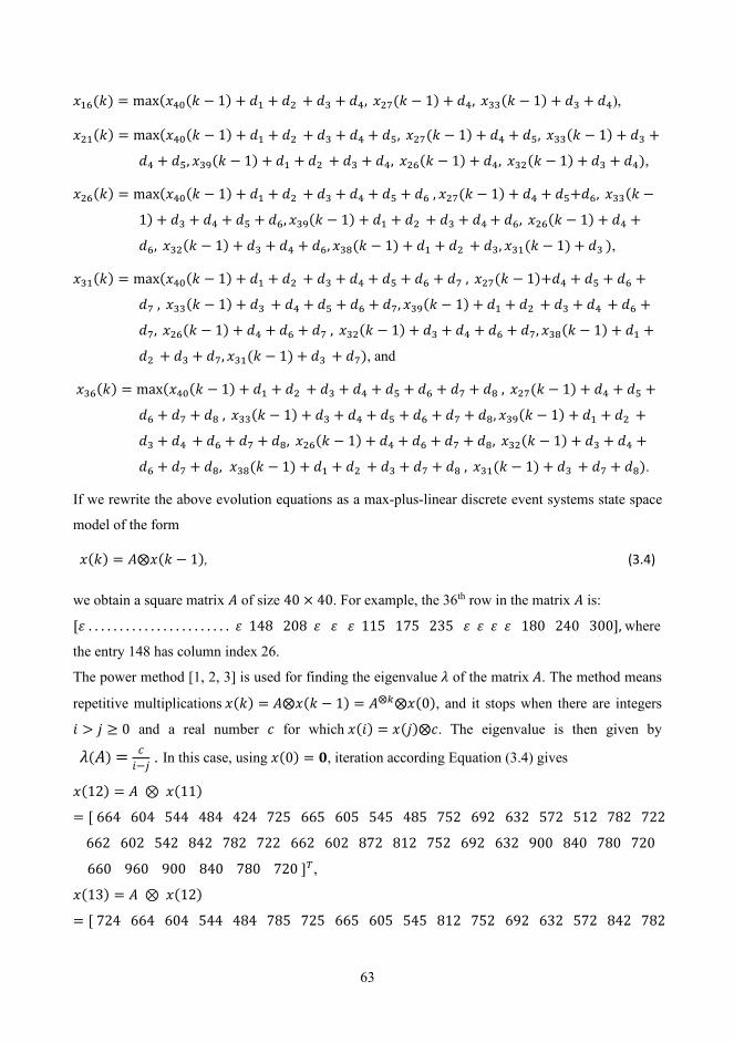
63

𝑥𝑥16(𝑘𝑘) = max(𝑥𝑥40(𝑘𝑘 − 1) + 𝑑𝑑1 + 𝑑𝑑2 + 𝑑𝑑3 + 𝑑𝑑4, 𝑥𝑥27(𝑘𝑘 − 1) + 𝑑𝑑4, 𝑥𝑥33(𝑘𝑘 − 1) + 𝑑𝑑3 + 𝑑𝑑4),

𝑥𝑥21(𝑘𝑘) = max(𝑥𝑥40(𝑘𝑘 − 1) + 𝑑𝑑1 + 𝑑𝑑2 + 𝑑𝑑3 + 𝑑𝑑4 + 𝑑𝑑5, 𝑥𝑥27(𝑘𝑘 − 1) + 𝑑𝑑4 + 𝑑𝑑5, 𝑥𝑥33(𝑘𝑘 − 1) + 𝑑𝑑3 +

𝑑𝑑4 + 𝑑𝑑5, 𝑥𝑥39(𝑘𝑘 − 1) + 𝑑𝑑1 + 𝑑𝑑2 + 𝑑𝑑3 + 𝑑𝑑4, 𝑥𝑥26(𝑘𝑘 − 1) + 𝑑𝑑4, 𝑥𝑥32(𝑘𝑘 − 1) + 𝑑𝑑3 + 𝑑𝑑4),

𝑥𝑥26(𝑘𝑘) = max(𝑥𝑥40(𝑘𝑘 − 1) + 𝑑𝑑1 + 𝑑𝑑2 + 𝑑𝑑3 + 𝑑𝑑4 + 𝑑𝑑5 + 𝑑𝑑6 , 𝑥𝑥27(𝑘𝑘 − 1) + 𝑑𝑑4 + 𝑑𝑑5+𝑑𝑑6, 𝑥𝑥33(𝑘𝑘 −

1) + 𝑑𝑑3 + 𝑑𝑑4 + 𝑑𝑑5 + 𝑑𝑑6, 𝑥𝑥39(𝑘𝑘 − 1) + 𝑑𝑑1 + 𝑑𝑑2 + 𝑑𝑑3 + 𝑑𝑑4 + 𝑑𝑑6, 𝑥𝑥26(𝑘𝑘 − 1) + 𝑑𝑑4 +

𝑑𝑑6, 𝑥𝑥32(𝑘𝑘 − 1) + 𝑑𝑑3 + 𝑑𝑑4 + 𝑑𝑑6, 𝑥𝑥38(𝑘𝑘 − 1) + 𝑑𝑑1 + 𝑑𝑑2 + 𝑑𝑑3, 𝑥𝑥31(𝑘𝑘 − 1) + 𝑑𝑑3 ),

𝑥𝑥31(𝑘𝑘) = max(𝑥𝑥40(𝑘𝑘 − 1) + 𝑑𝑑1 + 𝑑𝑑2 + 𝑑𝑑3 + 𝑑𝑑4 + 𝑑𝑑5 + 𝑑𝑑6 + 𝑑𝑑7 , 𝑥𝑥27(𝑘𝑘 − 1)+𝑑𝑑4 + 𝑑𝑑5 + 𝑑𝑑6 +

𝑑𝑑7 , 𝑥𝑥33(𝑘𝑘 − 1) + 𝑑𝑑3 + 𝑑𝑑4 + 𝑑𝑑5 + 𝑑𝑑6 + 𝑑𝑑7, 𝑥𝑥39(𝑘𝑘 − 1) + 𝑑𝑑1 + 𝑑𝑑2 + 𝑑𝑑3 + 𝑑𝑑4 + 𝑑𝑑6 +

𝑑𝑑7, 𝑥𝑥26(𝑘𝑘 − 1) + 𝑑𝑑4 + 𝑑𝑑6 + 𝑑𝑑7 , 𝑥𝑥32(𝑘𝑘 − 1) + 𝑑𝑑3 + 𝑑𝑑4 + 𝑑𝑑6 + 𝑑𝑑7, 𝑥𝑥38(𝑘𝑘 − 1) + 𝑑𝑑1 +

𝑑𝑑2 + 𝑑𝑑3 + 𝑑𝑑7, 𝑥𝑥31(𝑘𝑘 − 1) + 𝑑𝑑3 + 𝑑𝑑7), and

𝑥𝑥36(𝑘𝑘) = max(𝑥𝑥40(𝑘𝑘 − 1) + 𝑑𝑑1 + 𝑑𝑑2 + 𝑑𝑑3 + 𝑑𝑑4 + 𝑑𝑑5 + 𝑑𝑑6 + 𝑑𝑑7 + 𝑑𝑑8 , 𝑥𝑥27(𝑘𝑘 − 1) + 𝑑𝑑4 + 𝑑𝑑5 +

𝑑𝑑6 + 𝑑𝑑7 + 𝑑𝑑8 , 𝑥𝑥33(𝑘𝑘 − 1) + 𝑑𝑑3 + 𝑑𝑑4 + 𝑑𝑑5 + 𝑑𝑑6 + 𝑑𝑑7 + 𝑑𝑑8, 𝑥𝑥39(𝑘𝑘 − 1) + 𝑑𝑑1 + 𝑑𝑑2 +

𝑑𝑑3 + 𝑑𝑑4 + 𝑑𝑑6 + 𝑑𝑑7 + 𝑑𝑑8, 𝑥𝑥26(𝑘𝑘 − 1) + 𝑑𝑑4 + 𝑑𝑑6 + 𝑑𝑑7 + 𝑑𝑑8, 𝑥𝑥32(𝑘𝑘 − 1) + 𝑑𝑑3 + 𝑑𝑑4 +

𝑑𝑑6 + 𝑑𝑑7 + 𝑑𝑑8, 𝑥𝑥38(𝑘𝑘 − 1) + 𝑑𝑑1 + 𝑑𝑑2 + 𝑑𝑑3 + 𝑑𝑑7 + 𝑑𝑑8 , 𝑥𝑥31(𝑘𝑘 − 1) + 𝑑𝑑3 + 𝑑𝑑7 + 𝑑𝑑8).

If we rewrite the above evolution equations as a max-plus-linear discrete event systems state space

model of the form

𝑥𝑥(𝑘𝑘) = 𝐴𝐴⨂𝑥𝑥(𝑘𝑘 − 1), (3.4)

we obtain a square matrix 𝐴𝐴 of size 40 × 40. For example, the 36th row in the matrix 𝐴𝐴 is:

[𝜀𝜀 . . . . . . . . . . . . . . . . . . . . . . . 𝜀𝜀 148 208 𝜀𝜀 𝜀𝜀 𝜀𝜀 115 175 235 𝜀𝜀 𝜀𝜀 𝜀𝜀 𝜀𝜀 180 240 300], where

the entry 148 has column index 26.

The power method [1, 2, 3] is used for finding the eigenvalue 𝜆𝜆 of the matrix 𝐴𝐴. The method means

repetitive multiplications 𝑥𝑥(𝑘𝑘) = 𝐴𝐴⨂𝑥𝑥(𝑘𝑘 − 1) = 𝐴𝐴⨂𝑘𝑘⨂𝑥𝑥(0), and it stops when there are integers

𝑖𝑖 > 𝑗𝑗 ≥ 0 and a real number 𝑐𝑐 for which 𝑥𝑥(𝑖𝑖) = 𝑥𝑥(𝑗𝑗)⨂𝑐𝑐. The eigenvalue is then given by

𝜆𝜆(𝐴𝐴) = 𝑐𝑐𝑖𝑖−𝑗𝑗 . In this case, using 𝑥𝑥(0) = 𝟎𝟎, iteration according Equation (3.4) gives

𝑥𝑥(12) = 𝐴𝐴 ⊗ 𝑥𝑥(11)

= [ 664 604 544 484 424 725 665 605 545 485 752 692 632 572 512 782 722

662 602 542 842 782 722 662 602 872 812 752 692 632 900 840 780 720

660 960 900 840 780 720 ]𝑇𝑇,

𝑥𝑥(13) = 𝐴𝐴 ⊗ 𝑥𝑥(12)

= [ 724 664 604 544 484 785 725 665 605 545 812 752 692 632 572 842 782

64

722 662 602 902 842 782 722 662 932 872 812 752 692 960 900 840 780 720

1020 960 900 840 780 ]𝑇𝑇, and

𝑥𝑥(13) = 𝑥𝑥(12)⨂60.

Thus, the eigenvalue is 𝜆𝜆(𝐴𝐴) = 6013−12

= 60. The eigenvalue represents the cycle of the schedule,

which means that the trains start from each station every 60 minutes.

This also means that 𝑥𝑥(13) is an eigenvector, and (𝑥𝑥(13) − 𝑐𝑐), where 𝑐𝑐 is any constant, is also an

eigenvector. One eigenvector of 𝐴𝐴 is 𝑣𝑣, where

𝑣𝑣 = [0 −60 −120 −180 −240 61 1 −59 −119 − 179 88 28 −32 −92 −152 −118 58 −2 −62 − 122 178 118 58 − 2 −6 208 148 88 28 −32 236 176 116 56 − 2 296 236 176 116 56]𝑇𝑇.

(3.5)

This eigenvector 𝑣𝑣 includes the schedule of the trains, relative to the last departure from Helsinki (the

first element of 𝑣𝑣). Therefore, the element −240 means that five departures back a train from Helsinki

left 240 minutes ago, and the element 296 means that it takes 296 minutes for a train to come back to

Helsinki.

3.2 Delay Sensitivity Analysis

All the travel times 𝑑𝑑𝑖𝑖 introduced in Section 3.1 consist of a minimal travel time and a slack time.

Here it is assumed that the minimal travel time is 90% of the nominal time, and the slack is thus 10%.

For the small waiting time 𝑑𝑑1in Helsinki, it is assumed that there is no slack.

Handling delays is a relevant and common problem in train networks, and the sensitivity of delays

can be analyzed using max-plus models. A permanent delay means that the nominal travel times are

increased, which is compensated for by decreasing the other travel times to their minimal values. This

gives a slightly different system, for which a new eigenvalue can be calculated. The relative and

absolute limits for increasing the different traveling times individually without violation of the

roundtrip time (i.e. 𝜆𝜆 > T) are presented in Table 3.2.

Table 3.2: Delay sensitivity of the different traveling times.

Traveling time with delay 𝑑𝑑1 𝑑𝑑2 𝑑𝑑3 𝑑𝑑4 𝑑𝑑5 𝑑𝑑6 𝑑𝑑7 𝑑𝑑8

Relative limit 440% 18% 28% 10% 10% 10% 27.5% 19.3% Absolute limit (minutes) 17.6 11.5 7.8 3 6 3 7.7 11.6

Table 3.2 show the maximal value that a single traveling time 𝑑𝑑𝑖𝑖 can be increased, and still get the

nominal roundtrip time (given by the eigenvalue of the modified matrix) by decreasing all the other

traveling times to their minimal values. For example, if we increase 𝑑𝑑7 by 27.5%, which is equal to

65

7.7 minutes, and reduce all the other traveling times to their minimal values, we will still obtain the

eigenvalue 𝜆𝜆 = 60.

A limitation with the analysis is that it assumes a permanent change in the delays, and results concerns

only steady state. It does not give information about dynamic delay propagation, which is the theme

of the following section.

3.3 Dynamic Delay Propagation

The delay sensitivity analysis in Section 3.2 assumed that we had permanent changes in the traveling

times. A more normal situation is that the delay only concerns one single travel time, which means

that the corresponding max-plus system matrix becomes time varying, due to the fact that the travel

times 𝑑𝑑𝑖𝑖 become time varying (indicated by an index k). This is so due to the meeting conditions that

are Equations (3.1) and (3.2), where future states 𝑥𝑥𝐴𝐴𝑇𝑇(𝑘𝑘 + 1) and 𝑥𝑥𝐾𝐾𝑇𝑇(𝑘𝑘 + 2) appear. These are

expanded to max(𝑥𝑥𝐴𝐴𝐷𝐷(𝑘𝑘 − 4) + 𝑑𝑑1(𝑘𝑘 + 1) + 𝑑𝑑2(𝑘𝑘 + 1) + 𝑑𝑑3(𝑘𝑘 + 1) + 𝑑𝑑4(𝑘𝑘 + 1), 𝑥𝑥𝐾𝐾𝐾𝐾(𝑘𝑘 − 1) +

𝑑𝑑4(𝑘𝑘 + 1), 𝑥𝑥𝐾𝐾𝐷𝐷(𝑘𝑘 − 2) + 𝑑𝑑3(𝑘𝑘 + 1) + 𝑑𝑑4(𝑘𝑘 + 1)) and max(𝑥𝑥𝐴𝐴𝐷𝐷(𝑘𝑘 − 3) + 𝑑𝑑1(𝑘𝑘 + 2) + 𝑑𝑑2(𝑘𝑘 +

2) + 𝑑𝑑3(𝑘𝑘 + 2), 𝑥𝑥𝐾𝐾𝐷𝐷(𝑘𝑘 − 1) + 𝑑𝑑3(𝑘𝑘 + 2)) respectively. As indicated with iteration indices newer

versions of travel times are needed in these equations. Speeding up can also only be done after the

delay has appeared, which in our case means that after a delay in 𝑑𝑑𝑖𝑖(𝑘𝑘), only the traveling times

𝑑𝑑𝑖𝑖(𝑘𝑘), with 𝑗𝑗 > 𝑖𝑖, can be decreased in the same iteration k. In the next iteration, all the traveling times

can be decreased.

In Table 3.3, it has been tested how long it takes for a delay of 10, 20 and 30 minutes respectively in

a certain travel time, to disappear from the system.

Table 3.3: Times expressed in minutes that it takes for a delay in a certain traveling time to disappear from the system.

Travel Time Delay 10 min Delay 20 min Delay 30 min

𝑑𝑑1 89.2 182.4 301.3

𝑑𝑑2 88.3 182.4 300.4

𝑑𝑑3 93.2 182.4 300.4

𝑑𝑑4 91 185.1 303.1

𝑑𝑑5 91 185.1 303.1

𝑑𝑑6 93.2 182.4 300.4

𝑑𝑑7 68 184.2 305.3 𝑑𝑑8 89.2 182.4 301.3

66

The calculation of the disappearance of a delay can be done as follows. Let 𝑀𝑀𝑛𝑛 denote a matrix with

the nominal timetables, that is 𝑀𝑀𝑛𝑛 = [𝑣𝑣, 𝑣𝑣⨂𝑇𝑇, 𝑣𝑣⨂𝑇𝑇⨂2, … ], and Md is a matrix with the delayed

arrival and departure times at corresponding times. The part of the timetables that can be used for

selecting the part of the timetable that is affected by a delay using the logical expression(𝑀𝑀𝑑𝑑 −𝑀𝑀𝑛𝑛) >

0 . This means that the time instant of the last delay 𝑡𝑡𝑑𝑑 can be found using

𝑡𝑡𝑑𝑑 = max 𝑀𝑀𝑑𝑑(𝑀𝑀𝑑𝑑 −𝑀𝑀𝑛𝑛) > 0 − 𝑀𝑀𝑛𝑛(𝑖𝑖, 𝑗𝑗),

where i and j are the timetable indices when the actual first delay takes place. For example 88.3 in

Table 3 means that if the single traveling time 𝑑𝑑2 is increased by 10 minutes, and the traveling times

𝑑𝑑3, 𝑑𝑑4, 𝑑𝑑5, 𝑑𝑑6, 𝑑𝑑7 and 𝑑𝑑8 are speeded up to their minimal values, then the time instant of the last

deviation from the timetable is 88.3 minutes after the delay.

3.4 Recovery Matrix

In Goverde [25], max-plus linear systems are written in polynomial form,

𝑥𝑥(𝑘𝑘) = 𝐴𝐴0⨂𝑥𝑥(𝑘𝑘)⨁𝐴𝐴⨂𝑥𝑥(𝑘𝑘 − 1)⨁𝑤𝑤(𝑘𝑘), (3.6)

where 𝐴𝐴 is defined as in Equation (3.4), 𝐴𝐴0 is the matrix describing the direct connections from 𝑥𝑥(𝑘𝑘)

to 𝑥𝑥(𝑘𝑘), and 𝑤𝑤(𝑘𝑘) is the nominal departure times in period 𝑘𝑘.

𝐴𝐴0 is in this case given by all the direct traveling times 𝑑𝑑𝑖𝑖, including all delayed states, such that

𝐴𝐴0(𝑚𝑚 + 5,𝑚𝑚) = 𝑑𝑑𝑖𝑖, for 𝑚𝑚 = (𝑖𝑖 − 1)5 + 𝑛𝑛, for all 𝑛𝑛 = 1,2, … 5, and for all 𝑖𝑖 = 2, 3, … 8.

All the other elements of 𝐴𝐴0 are 𝜀𝜀, as there are no direct connections. The departure times are given

by the eigenvector 𝑣𝑣 in Equation (3.5), and the period 𝑇𝑇 according to 𝑤𝑤(𝑘𝑘) = 𝑇𝑇⨂𝑘𝑘⨂𝑣𝑣. The

polynomial equation can be written using a single matrix 𝐴𝐴𝑡𝑡, according to

𝑥𝑥(𝑘𝑘) = 𝐴𝐴𝑡𝑡⨂𝑥𝑥(𝑘𝑘 − 1)⨁𝑤𝑤(𝑘𝑘), (3.7)

where 𝐴𝐴𝑡𝑡 = 𝐴𝐴0⨁𝐴𝐴⨂𝑇𝑇⨂−1.

Definition: Consider the max-plus linear system in equation (3.7). The entry 𝑟𝑟𝑖𝑖𝑖𝑖 of the recovery matrix

𝑅𝑅 is defined as the maximum delay of 𝑥𝑥𝑖𝑖(𝑚𝑚) such that 𝑥𝑥𝑖𝑖(𝑘𝑘) is not delayed for any 𝑘𝑘 > 𝑚𝑚 [25]. The

following equation [2,4] defines the elements of the recovery matrix,

𝑟𝑟𝑖𝑖𝑖𝑖 = 𝑤𝑤𝑖𝑖 − 𝑤𝑤𝑖𝑖 − 𝐴𝐴𝑡𝑡+𝑖𝑖𝑖𝑖,

where the 𝑤𝑤𝑖𝑖 and 𝑤𝑤𝑖𝑖 are elements of vector 𝑤𝑤, 𝐴𝐴𝑡𝑡+ = ⨁𝑘𝑘=1∞ 𝐴𝐴𝑡𝑡⨂𝑘𝑘, and the notation 𝐴𝐴𝑡𝑡+𝑖𝑖𝑖𝑖 refers to the

ijth element of the matrix 𝐴𝐴𝑡𝑡+. If in the graph of 𝐴𝐴𝑡𝑡+ no path exists from node j to node i, then 𝑟𝑟𝑖𝑖𝑖𝑖 = ∞.

The recovery matrix, thus, takes values from the extended set ℝmax = ℝmax ∪ ∞.

67

In the studied train network between Helsinki and Turku, constructed from Table 3.1 presented in

Figure 3.1, the recovery matrix R is of size 40 × 40, with 𝑇𝑇 = 60. A 20 × 20 submatrix of that

matrix is given in Table 3.4.

Table 3.4: The upper left quadrant of the recovery matrix, with diagonal element shaded. 1 2 3 4 5 6 7 8 9 10 11 12 13 14 15 16 17 18 19 20

1 29.6 29.6 29.6 29.6 29.6 23.5 23.5 23.5 23.5 23.5 20.8 20.8 20.8 20.8 20.8 17.8 17.8 17.8 17.8 17.8

2 0 29.6 29.6 29.6 29.6 23.5 23.5 23.5 23.5 23.5 20.8 20.8 20.8 20.8 20.8 17.8 17.8 17.8 17.8 17.8

3 0 0 29.6 29.6 29.6 23.5 23.5 23.5 23.5 23.5 20.8 20.8 20.8 20.8 20.8 17.8 17.8 17.8 17.8 17.8

4 0 0 0 29.6 29.6 23.5 23.5 23.5 23.5 23.5 20.8 20.8 20.8 20.8 20.8 17.8 17.8 17.8 17.8 17.8

5 0 0 0 0 29.6 23.5 23.5 23.5 23.5 23.5 20.8 20.8 20.8 20.8 20.8 17.8 17.8 17.8 17.8 17.8

6 6.1 28.6 28.6 35.7 35.7 22.5 22.5 22.5 29.6 29.6 19.8 19.8 19.8 26.9 26.9 16.8 16.8 16.8 23.9 23.9

7 6.1 6.1 28.6 35.7 35.7 0 22.5 22.5 29.6 29.6 19.8 19.8 19.8 26.9 26.9 16.8 16.8 16.8 23.9 23.9

8 6.1 6.1 6.1 35.7 35.7 0 0 22.5 29.6 29.6 19.8 19.8 19.8 26.9 26.9 16.8 16.8 16.8 23.9 23.9

9 6.1 6.1 6.1 6.1 35.7 0 0 0 29.6 29.6 19.8 19.8 19.8 26.9 26.9 16.8 16.8 16.8 23.9 23.9

10 6.1 6.1 6.1 6.1 6.1 0 0 0 0 29.6 19.8 19.8 19.8 26.9 26.9 16.8 16.8 16.8 23.9 23.9

11 8.8 20.8 31.3 38.4 38.4 2.7 14.7 25.2 32.3 32.3 12 12 22.5 29.6 29.6 9 9 19.5 26.6 26.6

12 8.8 8.8 31.3 38.4 38.4 2.7 2.7 25.2 32.3 32.3 0 12 22.5 29.6 29.6 9 9 19.5 26.6 26.6

13 8.8 8.8 8.8 38.4 38.4 2.7 2.7 2.7 32.3 32.3 0 0 22.5 29.6 29.6 9 9 19.5 26.6 26.6

14 8.8 8.8 8.8 8.8 38.4 2.7 2.7 2.7 2.7 32.3 0 0 0 29.6 29.6 9 9 19.5 26.6 26.6

15 8.8 8.8 8.8 8.8 8.8 2.7 2.7 2.7 2.7 2.7 0 0 0 0 29.6 9 9 19.5 26.6 26.6

16 11.8 23.8 34.3 41.4 41.4 5.7 17.7 28.2 35.3 35.3 3 15 25.5 32.6 32.6 12 12 22.5 29.6 29.6

17 11.8 11.8 34.3 41.4 41.4 5.7 5.7 28.2 35.3 35.3 3 3 25.5 32.6 32.6 0 12 22.5 29.6 29.6

18 11.8 11.8 11.8 41.4 41.4 5.7 5.7 5.7 35.3 35.3 3 3 3 32.6 32.6 0 0 22.5 29.6 29.6

19 11.8 11.8 11.8 11.8 41.4 5.7 5.7 5.7 5.7 35.3 3 3 3 3 32.6 0 0 0 29.6 29.6

20 11.8 11.8 11.8 11.8 11.8 5.7 5.7 5.7 5.7 5.7 3 3 3 3 3 0 0 0 0 29.6

According to Goverde [25], the 𝑗𝑗𝑡𝑡ℎ column of the recovery matrix R gives the recovery time from

event j to all other events in the timetable and, thus, represents the impact a delay of event j has on

future train events, and the 𝑖𝑖𝑡𝑡ℎ row of the recovery matrix R gives the recovery time from event i from

all other events in the timetable and, thus, represents the sensitivity of event i on delays of preceding

events. The diagonal elements of R again represent recovery times to the event itself. In our example,

most of our states are delayed versions of previous states. As can be noted in Table 3.4, not all

diagonal elements representing the same departure at different times are the same.

For example 𝑟𝑟16,16 = 12, 𝑟𝑟18,18 = 22.5 and 𝑟𝑟19,19 = 29.6, although these elements all correspond

to the event “arrival in Turku” at times 𝑘𝑘, 𝑘𝑘 − 2 and 𝑘𝑘 − 3 respectively. As k is arbitrary, all these

recovery elements should logically be the same. This is not so because the delayed versions are just

memory variables, for which no other constraints than the back shifting according Equation 3.3 is

present and, thus, the recovery matrix is not correct for these. Thus, in our example only every fifth

row in the recovery matrix shows true recovery times, and these are shown in Table 3.5.

68

Table 3.5: The relevant parts of the recovery matrix. Diagonal elements highlighted with green, and recovery times related to a full cycle is highlighted with orange

1 2 3 4 5 6 7 8 9 10 11 12 13 14 15 16 17 18 19 20

1 29.6 29.6 29.6 29.6 29.6 23.5 23.5 23.5 23.5 23.5 20.8 20.8 20.8 20.8 20.8 17.8 17.8 17.8 17.8 17.8

6 6.1 28.6 28.6 35.7 35.7 22.5 22.5 22.5 29.6 29.6 19.8 19.8 19.8 26.9 26.9 16.8 16.8 16.8 23.9 23.9

11 8.8 20.8 31.3 38.4 38.4 2.7 14.7 25.2 32.3 32.3 12 12 22.5 29.6 29.6 9 9 19.5 26.6 26.6

16 11.8 23.8 34.3 41.4 41.4 5.7 17.7 28.2 35.3 35.3 3 15 25.5 32.6 32.6 12 12 22.5 29.6 29.6

21 17.8 29.8 40.3 41.4 47.4 11.7 23.7 34.2 35.3 41.3 9 21 31.5 32.6 38.6 6 18 28.5 29.6 35.6

26 20.8 32.8 38.4 44.4 50.4 14.7 26.7 32.3 38.3 44.3 12 24 29.6 35.6 41.6 9 21 26.6 32.6 38.6

31 23.6 35.6 41.2 47.2 53.2 17.5 29.5 35.1 41.1 47.1 14.8 26.8 32.4 38.4 44.4 11.8 23.8 29.4 35.4 41.4

36 29.6 41.6 47.2 53.2 59.2 23.5 35.5 41.1 47.1 53.1 20.8 32.8 38.4 44.4 50.4 17.8 29.8 35.4 41.4 47.4

21 22 23 24 25 26 27 28 29 30 31 32 33 34 35 36 37 38 39 40

1 11.8 11.8 11.8 11.8 11.8 8.8 8.8 8.8 8.8 8.8 6 6 6 6 6 0 0 0 0 0

6 10.8 10.8 10.8 17.9 17.9 7.8 7.8 7.8 14.9 14.9 5 5 5 12.1 12.1 6.1 6.1 6.1 6.1 6.1

11 3 3 13.5 20.6 20.6 0 0 10.5 17.6 17.6 7.7 7.7 7.7 14.8 14.8 8.8 8.8 8.8 8.8 8.8

16 6 6 16.5 23.6 23.6 3 3 13.5 20.6 20.6 10.7 10.7 10.7 17.8 17.8 11.8 11.8 11.8 11.8 11.8

21 6 12 22.5 23.6 29.6 3 9 19.5 20.6 26.6 10.7 10.7 16.7 17.8 23.8 11.8 11.8 11.8 11.8 17.8

26 3 15 20.6 26.6 32.6 6 12 17.6 23.6 29.6 7.7 13.7 14.8 20.8 26.8 8.8 8.8 8.8 14.8 20.8

31 5.8 17.8 23.4 29.4 35.4 2.8 14.8 20.4 26.4 32.4 10.5 16.5 17.6 23.6 29.6 11.6 11.6 11.6 17.6 23.6

36 11.8 23.8 29.4 35.4 41.4 8.8 20.8 26.4 32.4 38.4 6 22.5 23.6 29.6 35.6 17.6 17.6 17.6 23.6 29.6

The recovery matrix takes into consideration only one train, not the whole system, and it gives all the

information for the delay of one train only. A 0 in the recovery matrix means a tight schedule, with

no slack.

For example, the first row in the reduced recovery matrix is easy to interpret; the first value is 29.6,

which is the total slack for a single train. After that the slack is reduced by the slack in corresponding

travel time, up to the final value 0, which corresponds to that no slack is present in the 4-minute

waiting time in Helsinki (𝑑𝑑1). All the other traveling times are assumed to have 10% slack. The other

zero (row 11, column 26) is due to a meeting condition (in Salo).

The results shown in Table 3.2 can also be calculated using recovery matrix calculations. In Table

3.2, it was assumed that we have a permanent delay in one travel time. The maximum tolerance for a

permanent delay in one travel time can be obtained by increasing the corresponding travel time in the

recovery matrix, until we start obtaining negative entries on the relevant diagonal elements in the

recovery matrix (the ones indicated by green in Table 3.5).

The results in Table 3.5 can only partially be calculated using recovery matrix calculations. In Table

3.3, certain temporary delays (10, 20 and 30 minutes) were considered. In Table 3.3, it can be seen

that the time it takes for the system to catch up after delays of 30 minutes are all slightly more than

300 minutes. This is not a coincidence, as in most cases it is the delayed train itself that uses most

time to catch up, and the recovery time 29.6 in positions highlighted with orange means that if we

69

have a delay which is larger than 29.6, it will take more than 300 minutes (i.e. a full cycle) for the

system to catch up.

3.5 Conclusion

This chapter described how a max-plus model for a train system can be constructed. Meeting

conditions caused by having a single track, and other physical constrains, was handled by extending

the state space with delayed states, which has enabled rewriting the state update equation in the form

𝑥𝑥(𝑘𝑘) = 𝐴𝐴⊗𝑥𝑥(𝑘𝑘 − 1). Static and dynamic delay sensitivity of the network has been analyzed by

modifying the 𝐴𝐴-matrix and using eigenvalue calculations. The obtained results were compared to

standard recovery matrix-based calculations. A recovery matrix for the chosen extended state space

becomes large and contains even irrelevant information. Guidelines for finding and interpreting the

relevant information from the recovery matrix have been discussed. Max-plus formalism was used

throughout this chapter.

70

71

Chapter 4

Modeling and Scheduling of Production Systems

Scheduling of manufacturing systems is a difficult task, since they consist of many units with complex

relations and interdependences. In order to deal with this complexity, modeling and scheduling

techniques are used to guarantee that the whole production process is executed in a more dynamic

and reliable way than producing decisions manually. The questions of production scheduling in

manufacturing processes is becoming more important considering the increasing demand of

economic and environmental constraints. Therefore, in this chapter, we consider industrial production

scheduling problems for a manufacturing system consisting of parallel batch processes. These

processes can interact with each other and, therefore, influence the production of different batches in

these processes. These kinds of problems can be represented using discrete event systems, which in

general lead to a nonlinear description when using the conventional linear algebra. Therefore, we

suggest using the max-plus technique which results in systems that are “linear” in the max-plus

algebra. Scheduling of production systems is a common engineering problem, see for example Giffler

and Thompson [34]. Scheduling using max-plus algebra has also been studied in Baccelli et al. [1].

Because scheduling systems are linear in max-plus algebra, we can use more effective methods that

are available for modeling, simulation, and analysis of such systems. The production scheduling in a

manufacturing process consisting of 6 stages and 6 units done in parallel batches is consider as a case

study in this chapter.

The chapter is organized as follows. First, the scheduling problem is produced, formulation and

scheduling of a small production system consisting of 6 stages and 6 units is used as a case study and

modeling and simulation results for this problem are analyzed in Section 4.1. Section 4.2 presents the

analysis of the schedule of the production system. Asymptotic cases are studied in Sections 4.3 and

4.4, and Section 4.5 gives concluding remarks.

72

4.1 Manufacturing System

Consider the production system shown in Figure 4.1, the scheduling of which has been previously

studied by Björkqvist et al. [33] using optimization.

Figure 4.1: A manufacturing system

This manufacturing system consists of six processing stages A, B, C, D, E and F. Out of these, B and

C are performed in parallel, and D and E can overlap by 6 hours, otherwise the stages are performed

in order. Some of the stages have smaller capacities than the others, which means that they must be

performed more often, see Table 4.1.

Table 4.1: Specifications for the production stages in the manufacturing system.

Stages Processing time (h)

Cleaning time (h)

Durability (h)

Amount/batch (kg), repetitions/300kg in parenthesis

A B C D E F

7 4 7

10 8 1

4 2 2 4 4 0

48 60 60 24 24 48

300 (1) 50 (3) 75 (2) 150 (2) 150 (2) 150 (2)

For the stages, there are six different units, out of which units 1 and 2 can be used for stages A and

D, and units 3 and 4 can be used for stages B and C. The last two units can only be used for E and F

respectively. The reactors used for stage A and D are also used for temporary storage, which means

that the reactors cannot be used for another task before they are emptied. Half of the output from A

goes through B, and the other half goes through C. After stages B and C, temporary storages S1 and

S2 are used, gathering all intermediates needed for stage D. Stage E is performed overlapping with

stage D, so that stage D and E are performed for 6 hours in parallel. The final stage F must be

performed immediately after stage E has finished. The processing and cleaning times for stage N are

denoted 𝑃𝑃𝑁𝑁 and 𝑐𝑐𝑁𝑁 respectively and given in Table 4.1.

73

A central limiting factor for the production scheduling is the durability of the products produced in

stages B and C, which can only be stored for 60 hours. This means that the unit producing A should

be switched to production of D and, thus, the temporary storages S1 and S2 will be emptied.

4.1.1 A Max-plus Model for the Production System

Some simplifications were found necessary and/or appropriate. In particular, the following

assumptions were made:

1. Unit 3 is used only for stage B, and unit 4 is used only for stage C.

2. The temporary storages after B and C respectively are only limited by the storage time [33],

not by their size.

3. Scheduling of stage D is done based on the preliminary schedule obtained from the max-plus

model. The model is constructed so that it gives all the alternatives for stage D, and the final

schedule is obtained based on a set of simple rules.

4. Stages E and F are directly dependent on D, so the schedule for these are constructed based

on the selected schedule for D, and these are left out from the max-plus model. Normally E

and F simply follow D as they are faster than D, but when D is performed using both unit 1

and 2, E becomes the limiting factor. However, this can also be simply taken into account

when selecting the schedule for D.

5. Durability of the output from each stage is first ignored, as it can be shown that it does not

limit production of batches smaller than 4200kg. The durability constraints will play a major

role later, in the asymptotic analysis in Section 4.3.

The goal is to perform production as fast as possible, subject to all the constraints that are present.

This will now be formulated using a max-plus model, and for that, we need 10 states x, listed and

described below (where U𝑖𝑖 = Unit i):

1. U1 doing A

2. U2 doing D, step 1

3. U2 doing D, step 2

4. U3 doing B, step 1

5. U3 doing B, step 2

6. U3 doing B, step 3

7. U4 doing C, step 1

8. U4 doing C, step 2

74

9. U1 doing D, step 1

10. U1 doing D, step 2

Now we write down the max-plus-algebraic state space model of this production, with all the

constraints from the production and cleaning times included, in the equations that follow.

𝑥𝑥1(𝑘𝑘) = max (𝑥𝑥1(𝑘𝑘 − 1) + 𝑃𝑃𝐴𝐴, 𝑥𝑥5(𝑘𝑘 − 1) + 𝑃𝑃𝐵𝐵, 𝑥𝑥7(𝑘𝑘 − 1) + 𝑃𝑃𝐶𝐶)

𝑥𝑥2(𝑘𝑘) = max ( 𝑥𝑥3(𝑘𝑘 − 1) + 𝑃𝑃𝐷𝐷 , 𝑥𝑥5(𝑘𝑘) + 𝑃𝑃𝐵𝐵, 𝑥𝑥7(𝑘𝑘) + 𝑃𝑃𝐶𝐶)

𝑥𝑥3(𝑘𝑘) = max( 𝑥𝑥2(𝑘𝑘) + 𝑃𝑃𝐷𝐷 , 𝑥𝑥6(𝑘𝑘) + 𝑃𝑃𝐵𝐵, 𝑥𝑥8(𝑘𝑘) + 𝑃𝑃𝐶𝐶)

𝑥𝑥4(𝑘𝑘) = max (𝑥𝑥1(𝑘𝑘) + 𝑃𝑃𝐴𝐴, 𝑥𝑥6(𝑘𝑘 − 1) + 𝑃𝑃𝐵𝐵)

𝑥𝑥5(𝑘𝑘) = max (𝑥𝑥4(𝑘𝑘) + 𝑃𝑃𝐵𝐵)

𝑥𝑥6(𝑘𝑘) = max (𝑥𝑥5(𝑘𝑘) + 𝑃𝑃𝐵𝐵)

𝑥𝑥7(𝑘𝑘) = max (𝑥𝑥8(𝑘𝑘 − 1) + 𝑃𝑃𝐶𝐶 , 𝑥𝑥1(𝑘𝑘) + 𝑃𝑃𝐴𝐴)

𝑥𝑥8(𝑘𝑘) = max (𝑥𝑥7(𝑘𝑘) + 𝑃𝑃𝐶𝐶 )

𝑥𝑥9(𝑘𝑘) = max (𝑥𝑥6(𝑘𝑘) + 𝑐𝑐𝐴𝐴, 𝑥𝑥8(𝑘𝑘) + 𝑐𝑐𝐴𝐴)

𝑥𝑥10(𝑘𝑘) = max (𝑥𝑥9(𝑘𝑘) + 𝑃𝑃𝐷𝐷)

In order to obtain an equation of type

𝑥𝑥(𝑘𝑘) = 𝐴𝐴⨂𝑥𝑥(𝑘𝑘 − 1), (4.1)

the right-hand-side expressions containing 𝑘𝑘 or higher indices are substituted with expressions

containing index 𝑘𝑘 − 1 at most. After some straightforward (but tedious) algebraic manipulations and

simplifications, we obtain the following equations:

𝑥𝑥1(𝑘𝑘) = max (𝑥𝑥1(𝑘𝑘 − 1) + 𝑃𝑃𝐴𝐴, 𝑥𝑥5(𝑘𝑘 − 1) + 𝑃𝑃𝐵𝐵, 𝑥𝑥7(𝑘𝑘 − 1) + 𝑃𝑃𝐶𝐶)

𝑥𝑥2(𝑘𝑘) = max ( 𝑥𝑥1(𝑘𝑘 − 1) + 2𝑃𝑃𝐴𝐴 + 𝑘𝑘1, 𝑥𝑥3(𝑘𝑘 − 1) + 𝑃𝑃𝐷𝐷 , 𝑥𝑥5(𝑘𝑘 − 1) + 𝑃𝑃𝐴𝐴 + 𝑃𝑃𝐵𝐵 + 𝑘𝑘1, 𝑥𝑥6(𝑘𝑘 − 1)

+ 3𝑃𝑃𝐵𝐵 , 𝑥𝑥7(𝑘𝑘 − 1) + 𝑃𝑃𝐴𝐴 + 𝑃𝑃𝐶𝐶 + 𝑘𝑘1, 𝑥𝑥8(𝑘𝑘 − 1) + 2𝑃𝑃𝐶𝐶)

𝑥𝑥3(𝑘𝑘) = max( 𝑥𝑥1(𝑘𝑘 − 1) + 2𝑃𝑃𝐴𝐴 + 𝑘𝑘2, 𝑥𝑥3(𝑘𝑘 − 1) + 2𝑃𝑃𝐷𝐷 , 𝑥𝑥5(𝑘𝑘 − 1) + 𝑃𝑃𝐴𝐴 + 𝑃𝑃𝐵𝐵 + 𝑘𝑘2, 𝑥𝑥6(𝑘𝑘 − 1)

+ 3𝑃𝑃𝐵𝐵 + 𝑘𝑘3, 𝑥𝑥7(𝑘𝑘 − 1) + 𝑃𝑃𝐴𝐴 + 𝑃𝑃𝐶𝐶 + 𝑘𝑘2, 𝑥𝑥8(𝑘𝑘 − 1) + 2𝑃𝑃𝐶𝐶 + 𝑘𝑘4)

𝑥𝑥4(𝑘𝑘) = max (𝑥𝑥1(𝑘𝑘 − 1) + 2𝑃𝑃𝐴𝐴, 𝑥𝑥5(𝑘𝑘 − 1) + 𝑃𝑃𝐴𝐴 + 𝑃𝑃𝐵𝐵, 𝑥𝑥6(𝑘𝑘 − 1) + 𝑃𝑃𝐵𝐵 , 𝑥𝑥7(𝑘𝑘 − 1) + 𝑃𝑃𝐴𝐴 + 𝑃𝑃𝐶𝐶)

𝑥𝑥5(𝑘𝑘) = max (𝑥𝑥1(𝑘𝑘 − 1) + 2𝑃𝑃𝐴𝐴 + 𝑃𝑃𝐵𝐵 , 𝑥𝑥5(𝑘𝑘 − 1) + 𝑃𝑃𝐴𝐴 + 2𝑃𝑃𝐵𝐵, 𝑥𝑥6(𝑘𝑘 − 1) + 2𝑃𝑃𝐵𝐵, 𝑥𝑥7(𝑘𝑘 − 1) + 𝑃𝑃𝐴𝐴+ 𝑃𝑃𝐵𝐵 + 𝑃𝑃𝐶𝐶)

𝑥𝑥6(𝑘𝑘) = max (𝑥𝑥1(𝑘𝑘 − 1) + 2𝑃𝑃𝐴𝐴 + 2𝑃𝑃𝐵𝐵, 𝑥𝑥5(𝑘𝑘 − 1) + 𝑃𝑃𝐴𝐴 + 3𝑃𝑃𝐵𝐵, 𝑥𝑥6(𝑘𝑘 − 1) + 3𝑃𝑃𝐵𝐵, 𝑥𝑥7(𝑘𝑘 − 1) + 𝑃𝑃𝐴𝐴+ 2𝑃𝑃𝐵𝐵 + 𝑃𝑃𝐶𝐶)

75

𝑥𝑥7(𝑘𝑘) = max (𝑥𝑥1(𝑘𝑘 − 1) + 2𝑃𝑃𝐴𝐴, 𝑥𝑥5(𝑘𝑘 − 1) + 𝑃𝑃𝐴𝐴 + 𝑃𝑃𝐵𝐵, 𝑥𝑥7(𝑘𝑘 − 1) + 𝑃𝑃𝐴𝐴 + 𝑃𝑃𝐶𝐶 , 𝑥𝑥8(𝑘𝑘 − 1) + 𝑃𝑃𝐶𝐶)

𝑥𝑥8(𝑘𝑘) = max ( 𝑥𝑥1(𝑘𝑘 − 1) + 2𝑃𝑃𝐴𝐴 + 𝑃𝑃𝐶𝐶 , 𝑥𝑥5(𝑘𝑘 − 1) + 𝑃𝑃𝐴𝐴 + 𝑃𝑃𝐵𝐵 + 𝑃𝑃𝐶𝐶 , 𝑥𝑥7(𝑘𝑘 − 1) + 𝑃𝑃𝐴𝐴+ 2𝑃𝑃𝐶𝐶 , 𝑥𝑥8(𝑘𝑘 − 1) + 2𝑃𝑃𝐶𝐶)

𝑥𝑥9(𝑘𝑘) = max (𝑥𝑥1(𝑘𝑘 − 1) + 2𝑃𝑃𝐴𝐴 + 𝑐𝑐𝐴𝐴 + 𝑘𝑘1, 𝑥𝑥5(𝑘𝑘 − 1) + 𝑃𝑃𝐴𝐴 + 𝑃𝑃𝐵𝐵 + 𝑐𝑐𝐴𝐴 + 𝑘𝑘1, 𝑥𝑥6(𝑘𝑘 − 1) + 3𝑃𝑃𝐵𝐵+ 𝑐𝑐𝐴𝐴, 𝑥𝑥7(𝑘𝑘 − 1) + 𝑃𝑃𝐴𝐴 + 𝑃𝑃𝐶𝐶 + 𝑐𝑐𝐴𝐴 + 𝑘𝑘1, 𝑥𝑥8(𝑘𝑘 − 1) + 2𝑃𝑃𝐶𝐶 + 𝑐𝑐𝐴𝐴)

𝑥𝑥10(𝑘𝑘) = max ( 𝑥𝑥1(𝑘𝑘 − 1) + 2𝑃𝑃𝐴𝐴 + 𝑃𝑃𝐷𝐷 + 𝑐𝑐𝐴𝐴 + 𝑘𝑘1, 𝑥𝑥5(𝑘𝑘 − 1) + 𝑃𝑃𝐴𝐴 + 𝑃𝑃𝐵𝐵 + 𝑃𝑃𝐷𝐷 + 𝑐𝑐𝐴𝐴 + 𝑘𝑘1, 𝑥𝑥6(𝑘𝑘 −

1) + 3𝑃𝑃𝐵𝐵 + 𝑃𝑃𝐷𝐷 + 𝑐𝑐𝐴𝐴, 𝑥𝑥7(𝑘𝑘 − 1) + 𝑃𝑃𝐴𝐴 + 𝑃𝑃𝐶𝐶 + 𝑃𝑃𝐷𝐷 + 𝑐𝑐𝐴𝐴 + 𝑘𝑘1, 𝑥𝑥8(𝑘𝑘 − 1) + 2𝑃𝑃𝐶𝐶 + 𝑃𝑃𝐷𝐷 + 𝑐𝑐𝐴𝐴).

For simplicity, the following constants have been introduced in the above equations:

𝑘𝑘1 = max(2𝑃𝑃𝐵𝐵,𝑃𝑃𝐶𝐶), 𝑘𝑘2 = max(2𝑃𝑃𝐵𝐵 + 𝑃𝑃𝐷𝐷 , 3𝑃𝑃𝐵𝐵,𝑃𝑃𝐶𝐶 + 𝑃𝑃𝐷𝐷 , 2𝑃𝑃𝐶𝐶), 𝑘𝑘3 = max(𝑃𝑃𝐵𝐵,𝑃𝑃𝐷𝐷) and

𝑘𝑘4 = max(𝑃𝑃𝐶𝐶 ,𝑃𝑃𝐷𝐷). After introduction of numerical values from Table 4.1, the A-matrix of the

system becomes

𝐴𝐴 =

⎝

⎜⎜⎜⎜⎜⎜⎜⎜⎜⎜⎜⎛

7 𝜀𝜀 𝜀𝜀 𝜀𝜀 4 𝜀𝜀 7 𝜀𝜀 𝜀𝜀 𝜀𝜀

22 𝜀𝜀 𝜀𝜀 𝜀𝜀 19 12 22 14 𝜀𝜀 𝜀𝜀

32 𝜀𝜀 10 𝜀𝜀 29 22 32 30 𝜀𝜀 𝜀𝜀

14 𝜀𝜀 20 𝜀𝜀 11 4 14 𝜀𝜀 𝜀𝜀 𝜀𝜀

18 𝜀𝜀 𝜀𝜀 𝜀𝜀 15 8 18 𝜀𝜀 𝜀𝜀 𝜀𝜀

22 𝜀𝜀 𝜀𝜀 𝜀𝜀 19 12 22 𝜀𝜀 𝜀𝜀 𝜀𝜀

14 𝜀𝜀 𝜀𝜀 𝜀𝜀 11 𝜀𝜀 14 7 𝜀𝜀 𝜀𝜀

21 𝜀𝜀 𝜀𝜀 𝜀𝜀 18 𝜀𝜀 21 14 𝜀𝜀 𝜀𝜀

26 𝜀𝜀 𝜀𝜀 𝜀𝜀 23 16 26 18 𝜀𝜀 𝜀𝜀

36 𝜀𝜀 𝜀𝜀 𝜀𝜀 33 26 36 28 𝜀𝜀 𝜀𝜀 ⎠

⎟⎟⎟⎟⎟⎟⎟⎟⎟⎟⎟⎞

(4.2)

Normally, the cycle time of the discrete event system could be obtained from the eigenvalue of the

A-matrix, but this is not the case here. The reason for this is that the D-stages have a cycle time of 20,

while the others have a cycle time of 15. The graph corresponding to A is not strongly connected, i.e.,

A is not irreducible. It is, thus, not possible to calculate an eigenvector based on the matrix A in

Equation (4.2) This is due to the fact that there are no limits on the storage between production stages

B/C and D, so there is nothing synchronizing them. One can see this in Equation (4.2), columns 2, 3,

9 and 10: The states related to stages A, B and C, that is 1 and 4-8, are not constrained by the other

states related to stage D. Moreover, as the states related to D have a longer period, they will lag

behind, and are, thus, not constrained by the faster states.

76

4.2 Production Schedule from Iteration of the State Equation

The max-plus model is still useful for production scheduling by iteration of the state equation (4.1).

The initial state 𝑥𝑥(0) is set to 0, and 𝑥𝑥(𝑘𝑘) is given by Equation (4.1) using 𝐴𝐴 from Equation (4.2),

and with no B or u. As mentioned in Section 4.1, the results need to be interpreted in order to obtain

a close to optimal schedule:

1. The production is of batch type, so a certain number of repetitions of each stage are needed every

time. For all stages but D and E, this means that only the necessary number of steps is used from

the start of the schedule.

2. The schedule includes all possible D stages, most of them need to be discarded, based on the

following:

a) Unit 1 should finish all A-stages before switching to doing stage D. Thus, all scheduled D-

events based on states 9 and 10 prior to this should be discarded.

b) Out of the remaining D-stages, only the fastest up to the necessary number should be chosen.

3. The model does not include the limitation of the fact that the storages of B and C cannot be

negative. This is possible in the beginning when the storages are empty when A is started. In that

case, the first start of D cannot be earlier than 𝑃𝑃𝐴𝐴 + max(2𝑃𝑃𝐵𝐵,𝑃𝑃𝐶𝐶) (=15 hours in this case), and

the second start of D cannot be earlier than 𝑃𝑃𝐴𝐴 + max(3𝑃𝑃𝐵𝐵, 2𝑃𝑃𝐶𝐶) (=21 hours). In practice, this is

relevant in the case of a 300kg batch size for Unit 1, step 1 case (19 ⟶ 21 hours) and in the case

of a 600kg batch size for the second round of Unit 2, step 1 (35 ⟶ 36 hours).

4. The model does not contain limitations of stage E. E is only related to stage D, and it is necessary

that that previous E-stage needs to finish before contents of the D-stage can be moved to E. The

easy way to handle this constraint is to require that there is 𝑃𝑃𝐸𝐸 between each start of D. This

constraint becomes active after both unit 1 and 2 start doing stage D.

5. The schedule of E (unit 5) is always 𝑃𝑃𝐷𝐷 − 𝑃𝑃𝑂𝑂 after the end of the corresponding stage D.

In [33], four different batch sizes were considered: 300, 600, 900 and 1200 kg. The schedule for the

stages that are not related to stage D is obtained from the eigenvalue and the eigenvector of the matrix

where the states related to D (2, 3, 9 and 10) are left out.

This results in the eigenvalue of 15 and eigenvector of [0 7 11 15 7 14]𝑇𝑇. This means that

each unit should be started according to the eigenvector plus a multiple of 15. The schedule for the

D-stages is obtained from the preliminary schedule using point 2a and 2b. The capacity of stage D is

77

150 kg, so 2, 4, 6 and 8 stages of D respectively are needed in the four considered cases. The relevant

states are 2, 3, 9 and 10, and the schedule for these are shown in Table 4.2.

Table 4.2: Preliminary production schedule for stage D. Numbers in parenthesis and red are

discarded as unit 1 is still needed for stage A, and numbers in blue and with a * are

discarded as they are excessive.

Batch size 300kg 600kg 900kg 1200kg

Unit 2, step 1 15 15 35 15 35 55 15 35 55 75*

Unit 2, step 2 25* 25 45* 25 45 65* 25 45 65 85*

Unit 1, step 1 19 (19) 34 (19) (34) 49 (19) (34) (49) 64

Unit 1, step 2 29* (29) 44* (29) (44) 59* (29) (44) (59) 74

On top of that the constraint related to stage E, that is the time between the start of a unit producing

D should not be less than 8, is enforced. This affects all the events starting from the first-time

producing D using unit 1, which can be seen in Table 4.3a, where the final schedule for D is given.

Table 4.3a. Final production schedule for stage D including the constraint for E, meaning in this

case that there must be 8 hours between each start of D. Unit 2 in black, unit 1 in red and

marked with a *. The constraints from B and C storages do not become active for so small

batches.

Batch size stage 1 stage 2 stage 3 stage 4 stage 5 stage 6 stage 7 stage 8

300kg 15 23*

600kg 15 25 34* 42

900kg 15 25 35 45 53* 61

1200kg 15 25 35 45 55 64* 72 80*

Production times and rates for the different batches are given in Table 4.3b.

Table 4.3b. Production rate for different productions Production 300 600 900 1200 1500 1800 2100 2400 2700 3000 3300 3600 3900 4200 Prod. time 42 61 80 99 118 137 156 175 194 213 232 251 270 289 Prod. rate 7.14 9.84 11.25 12.12 12.71 13.14 13.46 13.71 13.92 14.08 14.22 14.34 14.44 14.53

As can be seen from Table 4.3b, the production time in increased with 19 hours for each addition of

300 kg of production, so one can conjecture that the production rate will converge towards 30019

kg/h.

78

4.3 Asymptotic Case

With the asymptotic case we mean scheduling of very large (unlimited) batches so that the durability

constraints need to be considered. The asymptotic production consists of two stages related to the

storage of B and C: the filling stage and the emptying stage. The asymptotic production cases are

introduced below with a graph of each case. A typical process involves A, B, C, D stages, as already

mentioned in Section 4.1.

In the filling stage, the initial production schedule, presented in Section 4.2, accumulates B and C in

storages. Accumulation is due to the fact that A is produced at a rate of 300kg/15h, and D at a

minimum production rate of 300kg/20 hours. A simple but suboptimal strategy is to delay the

production of A, so that it also produces at a rate 300kg/20h = 15kg/h and, thus, avoid the

accumulation of B and C storages. However, it is beneficial to clean the unit used for production of

A and produce D using two units, resulting in a production rate of 300kg/16h. Thus, the scheduling

of the production can be seen as switching between the mode where only one unit is used for

production of D, and the mode where two units are used for production of D. In the first mode, the

total production is limited by the production of D, and the production rate is 𝑟𝑟1 = 150/10. In the

second mode, the total production will be limited by the production of E, when the production rate is

𝑟𝑟2 = 150/8. The actual production rate 𝑟𝑟𝑡𝑡 will be a with production times weighted average of 𝑟𝑟1 and

𝑟𝑟2, that is

𝑟𝑟𝑡𝑡 = (𝑡𝑡𝑑𝑑1 ∙ 𝑟𝑟1 + 𝑡𝑡𝑑𝑑2 ∙ 𝑟𝑟2) ∙1𝑝𝑝

,

where 𝑝𝑝 = 𝑡𝑡𝑑𝑑1 + 𝑡𝑡𝑑𝑑2 + 2𝑡𝑡𝑐𝑐 is the period of production, and 𝑡𝑡𝑑𝑑1 is the time for production using only

one unit for D, 𝑡𝑡𝑑𝑑2 is the time for production using two units for D, and 𝑡𝑡𝑐𝑐 is the cleaning time. Now

𝑡𝑡𝑑𝑑2 = 𝑡𝑡𝑑𝑑1∙𝑟𝑟𝑎𝑎𝑟𝑟2

asymptotically, where 𝑟𝑟𝑚𝑚 is the accumulation rate.

The production rate will be

𝑟𝑟𝑡𝑡 =𝑡𝑡𝑑𝑑1 ∙ 𝑟𝑟1 + (𝑡𝑡𝑑𝑑1 ∙ 𝑟𝑟𝑚𝑚𝑟𝑟2

) ∙ 𝑟𝑟2𝑝𝑝

=𝑡𝑡𝑑𝑑1 ∙ 𝑟𝑟1 + 𝑡𝑡𝑑𝑑1 ∙ 𝑟𝑟𝑚𝑚

𝑝𝑝,

which can be differentiated with respect to 𝑡𝑡𝑑𝑑1, and

𝜕𝜕𝑟𝑟𝑡𝑡𝜕𝜕𝑡𝑡𝑑𝑑1

=(𝑟𝑟1 + 𝑟𝑟𝑚𝑚) ∙ 𝑡𝑡𝑑𝑑2 + (𝑟𝑟1 + 𝑟𝑟𝑚𝑚) ∙ 2𝑡𝑡𝑐𝑐

𝑝𝑝2> 0.

79

The last inequality follows as all the times and rates are positive, which means that 𝑡𝑡𝑑𝑑1 should be

chosen as large as possible, that is at the durability constraint. Both B and C have a durability of 60

hours, and this is the durability constraint that should be the target for the schedule.

Production schedules can be obtained using max-plus for both the filling and the emptying phase.

Switching between these phases cannot be done using max-plus, but it is easily done by keeping track

of the B and C storages. Switching can be carried out after a certain number of repetitions of A in the

filling stage and after a certain number of repetitions of D in the emptying stage. The schedule after

the switch can be initialized based on the previous schedule.

The long-term production consists of two different modes:

1. One of the units 1 or 2 is used for production of A, and the other is used for production of D.

In this mode B and C are accumulated in the storages. The length of this mode is characterized

by the number of repetitions of A, denoted 𝑛𝑛𝐴𝐴.

2. Both units 1 and 2 are used for production of D, when the storages of B and C are emptied.

The length of this mode is characterized by the number of repetitions of D, denoted 𝑛𝑛𝐷𝐷.

Scheduling of the long-term production essentially consists of the choice of these repetitions 𝑛𝑛𝐴𝐴 and

𝑛𝑛𝐷𝐷. The choice of 𝑛𝑛𝐴𝐴 affects the storage times, the more repetitions the more accumulation in the

storages, and the longer time for emptying it. The choice of 𝑛𝑛𝐷𝐷 is bound to the choice of 𝑛𝑛𝐴𝐴, as the

storages need to be sufficiently emptied before restart of production of A. It can be shown that 𝑛𝑛𝐴𝐴

should be about twice the 𝑛𝑛𝐷𝐷. The storages will build up during production of A at a rate

300kg15h

−300kg

20h= 5 kg/h

The storages will be emptied at a rate 150/8 kg/h during usage of two D-units. An A-repetition takes

15 hours, and a D-repetition takes 8 hours, and putting equality for buildup and emptying gives

𝑛𝑛𝐴𝐴 ∙ 15h ∙ 5kg/h = 𝑛𝑛𝐷𝐷 ∙ 8h ∙150

8kg/h

𝑛𝑛𝐴𝐴𝑛𝑛𝐷𝐷

=15075

= 2

One can choose to repeat the D-production one time more than necessary, as this reduces the storage

times, with a cost of having the D-production unit idle for a while at the beginning of the next mode

1. However, this increases the period length and reduces the overall production rate. Table 4.4 lists

the results for different choices of 𝑛𝑛𝐴𝐴 and 𝑛𝑛𝐷𝐷.

80

3. The 𝑛𝑛𝐴𝐴 − 𝑛𝑛𝐷𝐷 cycle must be eventually periodic. It is uniquely determined by the storage in

B and C at the beginning of the 𝑛𝑛𝐴𝐴 stage, and there are only a finite number of possibilities

for those.

For example, if the storages are empty when the 𝑛𝑛𝐴𝐴 stage starts, the process is periodic from the

beginning (as when 𝑛𝑛𝐴𝐴 = 15 and 𝑛𝑛𝐷𝐷= 8, cf. Fig. 4.5).

Table 4.4. Periods, storage times and production rates for long-term strategies for different number

of A- and D-repetitions.

𝑛𝑛𝐴𝐴 𝑛𝑛𝐷𝐷 Period (h)

Maximum storage times for B and C (h)

Production rate (kg/h)

Figure

12 6 230 50 15.65

12 7 238 48 15.13

13 6 249 54 15.66

13 7 257 52 15.18

14 7 268 58 15.67 4.2 and 4.3

14 8 276 56 15.22

15 7 287 62 15.68 4.4

15 8 295 60 15.25 4.5

16 8 306 66 15.69

16 9 314 64 15.29

As can be seen in Table 4.4, the production rate does not increase monotonically as a function of 𝑛𝑛𝐴𝐴,

which depends on the fact that the switches are better timed in the cases with an even number of A-

steps. As can be seen from the table, the number of D-steps is the same in odd numbered A-steps as

in the previous even numbered case. In addition, the production is larger during the D-steps (when

both units are used for production of D, with a rate 150/8=18.75kg/h) than during A-steps (when only

one unit is used for D, with a production of 15kg/h). In our case, the limit for the storage times is 60

hours, and the most relevant schedules are illustrated in Figures 4.2-4.4.

81

Figure 4.2. Optimal schedule with maximum storage time 58 hours from the start. The period

is 268 hours, and the periodicity starts at 𝑡𝑡 = 3 hours. Production rate

15.67kg/hours.

Figure 4.3. The first 1000 hours of the schedule in Figure 4.2.

0 200 400 600 800 1000 1200 1400 1600 1800 2000

0

100

200

300

400

500

600

Time t (h)

Stor

age

(kg)

Storage of B

Storage of C

0 100 200 300 400 500 600 700 800 900 10000

100

200

300

400

500

600

Time t (h)

Sto

rage

(kg)

Storage of B

Storage of C

82

Figure 4.4. Optimal schedule with maximum storage time 62 hours from the start. The period

is 287 hours, and the periodicity starts at 𝑡𝑡 = 3 hours. Production rate

15.68kg/hour.

Figure 4.5. Schedule with delayed switch from D to A, resulting in eleven hours waiting for

the other D producing unit at each cycle. The period is the 295 hours, and the

periodicity starts in the beginning. Production rate 15.25kg/hours

0 100 200 300 400 500 600 700 800 900 10000

100

200

300

400

500

600

Time t (h)

Sto

rage

(kg)

Storage of B

Storage of C

0 100 200 300 400 500 600 700 800 900 10000

100

200

300

400

500

600

Time t (h)

Sto

rage

(kg)

Storage of B

Storage of C

83

Figure 4.5 results in a worse production rate than in Figure 4.3, and it is not possible to improve on

this by increasing the A-steps. As can be seen from Table 4.4, it will result in violation of the

durability constraint.

Increasing the storage time seems to converge to the production rate 300/19 as conjectured after Table

4.3b, which can be seen in Table 4.5 and Figure 4.6.

Table 4.5. Numerical test of upper limit on production rate.

Storage time Production rate 58 15.67 114 15.73 230 15.76 462 15.775 926 15.782 1854 15.786 3710 15.7877 7422 15.78886 14846 15.789026 29694 15.789250 59390 15.789362 ∞ 300/19 ≈ 15.789474

Figure. 4.6. Actual production rates as function of allowed storage times, and the presumed limit

300/19 for the production rate.

0 10000 20000 30000 40000 50000 6000015.779

15.780

15.781

15.782

15.783

15.784

15.785

15.786

15.787

15.788

15.789

15.790

Storage time (h)

Pro

duct

ion

rate

(kg/

h)

actual rates

300/19

84

4.4 Asymptotic Case Using Max-plus

The asymptotic production consists of two stages, one filling stage and one emptying stage. Three

different max-plus models are formulated, describing different parts of the system:

M1. The production of A, B, and C, used in the filling stage

M2. The production of D and E using only one of the units for D, during the filling stage

M3. The production of D and E using both units for D, during the emptying stage

Between the filling and the emptying stage there is a switch, where production of A, B, and C is

ended, and the unit producing A is cleaned and used for production of D. This means that the

production of D is switched from M2 to M3, and that the state of M3 is initialized using M1 and/or

M2 (depending on if the cleaned A-producing unit from M1 or the D-producing unit from M2 is the

first available to start M3). Between emptying there is also a switch, where one of the units used for

production of D is cleaned, and production of A, that is M1, is started. Furthermore, M3 is switched

to M2. The states of M1 and M2 are both initialized using states of M3.

4.4.1 Production of A, B, and C, M1

This system consists of three processing stages A, B, and C. Out of these B and C are performed in

parallel. For the stages, there are three different units, out of which unit 1 can be used for stage A and

unit 3 can be used for stages B with three steps. Unit 4 can only be used for C with two steps. This

will now be formulated using a max-plus model, and for that, we need 6 states 𝑥𝑥𝑖𝑖, listed and described

below:

Filling stages 1. U1 doing A

2. U3 doing B, step 1

3. U3 doing B, step 2

4. U3 doing B, step 3

5. U4 doing C, step 1

6. U4 doing C, step 2

Now we write down the max-plus-algebraic state space model of this DES.

𝑥𝑥1(𝑘𝑘) = max (𝑥𝑥1(𝑘𝑘 − 1) + 𝑃𝑃𝐴𝐴, 𝑥𝑥3(𝑘𝑘 − 1) + 𝑃𝑃𝐵𝐵, 𝑥𝑥5(𝑘𝑘 − 1) + 𝑃𝑃𝐶𝐶)

𝑥𝑥2(𝑘𝑘) = max (𝑥𝑥1(𝑘𝑘 − 1) + 2𝑃𝑃𝐴𝐴, 𝑥𝑥3(𝑘𝑘 − 1) + 𝑃𝑃𝐴𝐴 + 𝑃𝑃𝐵𝐵, 𝑥𝑥4(𝑘𝑘 − 1) + 𝑃𝑃𝐵𝐵 , 𝑥𝑥5(𝑘𝑘 − 1) + 𝑃𝑃𝐴𝐴 + 𝑃𝑃𝐶𝐶)

85

𝑥𝑥3(𝑘𝑘) = max (𝑥𝑥1(𝑘𝑘 − 1) + 2𝑃𝑃𝐴𝐴 + 𝑃𝑃𝐵𝐵 , 𝑥𝑥3(𝑘𝑘 − 1) + 𝑃𝑃𝐴𝐴 + 2𝑃𝑃𝐵𝐵, 𝑥𝑥4(𝑘𝑘 − 1) + 2𝑃𝑃𝐵𝐵, 𝑥𝑥5(𝑘𝑘 − 1) + 𝑃𝑃𝐴𝐴+ 𝑃𝑃𝐵𝐵 + 𝑃𝑃𝐶𝐶)

𝑥𝑥4(𝑘𝑘) = max (𝑥𝑥1(𝑘𝑘 − 1) + 2𝑃𝑃𝐴𝐴 + 2𝑃𝑃𝐵𝐵, 𝑥𝑥3(𝑘𝑘 − 1) + 𝑃𝑃𝐴𝐴 + 3𝑃𝑃𝐵𝐵, 𝑥𝑥4(𝑘𝑘 − 1) + 3𝑃𝑃𝐵𝐵, 𝑥𝑥5(𝑘𝑘 − 1) + 𝑃𝑃𝐴𝐴+ 2𝑃𝑃𝐵𝐵 + 𝑃𝑃𝐶𝐶)

𝑥𝑥5(𝑘𝑘) = max (𝑥𝑥1(𝑘𝑘 − 1) + 2𝑃𝑃𝐴𝐴, 𝑥𝑥3(𝑘𝑘 − 1) + 𝑃𝑃𝐴𝐴 + 𝑃𝑃𝐵𝐵, 𝑥𝑥5(𝑘𝑘 − 1) + 𝑃𝑃𝐴𝐴 + 𝑃𝑃𝐶𝐶 , 𝑥𝑥6(𝑘𝑘 − 1) + 𝑃𝑃𝐶𝐶)

𝑥𝑥6(𝑘𝑘) = max ( 𝑥𝑥1(𝑘𝑘 − 1) + 2𝑃𝑃𝐴𝐴 + 𝑃𝑃𝐶𝐶 , 𝑥𝑥3(𝑘𝑘 − 1) + 𝑃𝑃𝐴𝐴 + 𝑃𝑃𝐵𝐵 + 𝑃𝑃𝐶𝐶 , 𝑥𝑥5(𝑘𝑘 − 1) + 𝑃𝑃𝐴𝐴+ 2𝑃𝑃𝐶𝐶 , 𝑥𝑥6(𝑘𝑘 − 1) + 2𝑃𝑃𝐶𝐶)

After introduction of numerical values from Table 4.1, the A-matrix of the system becomes as follows:

𝐴𝐴 =

⎝

⎜⎜⎛

7 𝜀𝜀 414 𝜀𝜀 1118 𝜀𝜀 15

𝜀𝜀 7 𝜀𝜀4 14 𝜀𝜀8 18 𝜀𝜀

22 𝜀𝜀 1914 𝜀𝜀 1121 𝜀𝜀 18

12 22 𝜀𝜀𝜀𝜀 14 7𝜀𝜀 21 14⎠

⎟⎟⎞

(4.3)

The eigenvalue of the A-matrix is 15 and the eigenvector is [0 7 11 15 7 14]𝑇𝑇 .

4.4.2 Production of D and E Using Only One of the Units for D, M2

This system consists of two processing stages D and E. For the stages, there are two different units,

out of which unit 1 can be used for stage D, and unit 5 can be used for stages E. In this case, unit 2 is

used for production of A. This will now be formulated using a max-plus model, and for that, we need

2 states 𝑥𝑥𝑖𝑖, listed and described below.

Filling stages

1. U1 doing D

2. U5 doing E

Now we write down the max-plus-algebraic state space model of this DES.

𝑥𝑥1(𝑘𝑘) = max ( 𝑥𝑥1(𝑘𝑘 − 1) + 𝑃𝑃𝐷𝐷 , 𝑥𝑥2(𝑘𝑘 − 1) + 𝑃𝑃𝐸𝐸 − 𝑃𝑃𝐷𝐷 + 𝑃𝑃𝑜𝑜)

𝑥𝑥2(𝑘𝑘) = max(𝑥𝑥1(𝑘𝑘 − 1) + 2𝑃𝑃𝐷𝐷 − 𝑃𝑃𝑜𝑜), 𝑥𝑥2(𝑘𝑘 − 1) + 𝑃𝑃𝐸𝐸)

After introduction of numerical values from Table 4.1, the A-matrix of the system becomes

𝐴𝐴 = 10 4

14 8. (4.4)

The eigenvalue of the A-matrix is 10 and the eigenvector is [0 4]𝑇𝑇

86

4.4.3 Production of D and E Using Both Units for D, M3

This system consists of two processing stages D, E, and F (see Figure 4.7). Stage F is not modeled,

as it follows directly after E, and is so fast that it does not constrain anything. For the other stages,

there are three different units, out of which units 1 and 2 can be used for stage D, and unit 5 can be

used for stages E with two steps.

Figure 4.7: System in emptying mode

This will now be formulated using a max-plus model, and for that, we need 4 states 𝑥𝑥𝑖𝑖, listed and

described below:

Stages for emptying cycle

1. U1 doing D

2. U2 doing D

3. U5 doing E, step 1

4. U5 doing E, step 2

The production of E is modeled using two states, modeling which D production unit is currently

served.

Now we write down the max-plus-algebraic state space model of this DES.

𝑥𝑥1(𝑘𝑘) = max ( 𝑥𝑥1(𝑘𝑘 − 1) + 𝑃𝑃𝐷𝐷 , 𝑥𝑥4(𝑘𝑘 − 1) + 𝑃𝑃𝐸𝐸 − 𝑃𝑃𝐷𝐷 + 𝑃𝑃𝑜𝑜)

𝑥𝑥2(𝑘𝑘) = max(𝑥𝑥1(𝑘𝑘) + 𝑃𝑃𝐷𝐷 − 𝑃𝑃𝑜𝑜)

𝑥𝑥3(𝑘𝑘) = max (𝑥𝑥3(𝑘𝑘 − 1) + 𝑃𝑃𝐷𝐷 , 𝑥𝑥2(𝑘𝑘) + 𝑃𝑃𝐸𝐸 − 𝑃𝑃𝐷𝐷 + 𝑃𝑃𝑜𝑜)

𝑥𝑥4(𝑘𝑘) = max( 𝑥𝑥3(𝑘𝑘) + 𝑃𝑃𝐷𝐷 − 𝑃𝑃𝑜𝑜)

In order to obtain an equation of type 𝑥𝑥(𝑘𝑘) = 𝐴𝐴⨂𝑥𝑥(𝑘𝑘 − 1), the right-hand-side expressions

containing 𝑘𝑘 or higher indices are substituted with expressions containing index 𝑘𝑘 − 1 at most. After

some straightforward algebraic manipulations and simplifications, we obtain the following equations:

𝑥𝑥1(𝑘𝑘) = max ( 𝑥𝑥1(𝑘𝑘 − 1) + 𝑃𝑃𝐷𝐷 , 𝑥𝑥4(𝑘𝑘 − 1) + 𝑃𝑃𝐸𝐸 − 𝑃𝑃𝐷𝐷 + 𝑃𝑃𝑜𝑜)

87

𝑥𝑥2(𝑘𝑘) = max(𝑥𝑥1(𝑘𝑘 − 1) + 2𝑃𝑃𝐷𝐷 − 𝑃𝑃𝑜𝑜 , 𝑥𝑥4(𝑘𝑘 − 1) + 𝑃𝑃𝐸𝐸)

𝑥𝑥3(𝑘𝑘) = max (𝑥𝑥1(𝑘𝑘 − 1) + 𝑃𝑃𝐷𝐷 + 𝑃𝑃𝐸𝐸 , 𝑥𝑥3(𝑘𝑘 − 1) + 𝑃𝑃𝐷𝐷 , 𝑥𝑥4(𝑘𝑘 − 1) + 2𝑃𝑃𝐸𝐸 − 𝑃𝑃𝐷𝐷 + 𝑃𝑃𝑜𝑜)

𝑥𝑥4(𝑘𝑘) = max( 𝑥𝑥1(𝑘𝑘 − 1) + 2𝑃𝑃𝐷𝐷 + 𝑃𝑃𝐸𝐸 − 𝑃𝑃𝑜𝑜 , 𝑥𝑥3(𝑘𝑘 − 1) + 2𝑃𝑃𝐷𝐷 − 𝑃𝑃𝑜𝑜 , 𝑥𝑥4(𝑘𝑘 − 1) + 2𝑃𝑃𝐸𝐸)

After introduction of numerical values from Table 4.1, the A-matrix of the system becomes

𝐴𝐴 = 10 𝜀𝜀 𝜀𝜀 4141822

𝜀𝜀𝜀𝜀𝜀𝜀

𝜀𝜀1014

81216

. (4.5)

The eigenvalue of the A-matrix is 16 where the eigenvector is [0 4 8 12]𝑇𝑇. Schedules produced

by using simulations of the three models are shown in Tables 4.6 to 4.8. As can be seen in Tables 4.6

to 4.8, we use the choice of 𝑛𝑛𝐴𝐴 = 14 and 𝑛𝑛𝐷𝐷 = 7 and the period length is 268 hours.

Table 4.6: Schedule for units producing A, B and C according to model M1. In the last round, the

start of B3 (highlighted with yellow) liberates A for cleaning (which takes 4 hours) and

gives the starting time of D1 in Table 4.8. The cells highlighted with orange are the ones

initialized by the orange cells in Table 4.8

Step index 1 2 3 … 14 15 16 … 28 29 30 … 42 43 44 …

A 0 15 30 … 195 268 283 … 463 536 551 … 731 804 819 …

B1 7 22 37 … 202 275 290 … 470 543 558 … 738 811 826 …

B2 11 26 41 … 206 279 294 … 474 547 562 … 742 815 830 …

B3 15 30 45 … 210 283 298 … 478 551 566 … 746 819 834 …

C1 7 22 37 … 202 275 290 … 470 543 558 … 738 811 826 …

C2 14 29 44 … 209 282 297 … 477 550 565 … 745 818 833 …

Table 4.6 shows that the production, also seen in Figure 4.3, is periodic from the start. The period

length is 268 hours, which is the difference between the numbers in the orange cells, which indicates

the restarting times for production of A. Table 4.7 gives the schedule for the production of D and E,

and the same period 268 hours can be seen between the switching time instances highlighted with

green cells. Table 4.8 gives the schedule for the production of D and E, using two units for D. The

schedule becomes periodic starting from iteration 21, and the period length of 268 hours can again be

seen between the switching time instances highlighted with yellow and green respectively.

88

Table 4.7: Schedule for units producing D and E according to model M2. The cells highlighted

with green are the ones initialized by the green cells in Table 4.8

Step index 1 2 3 4 … 20 21 22 … 41 42 43 …

D 15 25 35 45 … 205 272 282 … 472 540 550 …

E 19 29 39 49 … 209 276 286 … 476 544 554 …

Table 4.8: Schedule for units producing D and E according to model M3. The cells highlighted

with yellow are the ones initialized by the yellow cells in Table 4.6. The start of the last round of

D2, highlighted with orange, is after completion (10 hours) and cleaning (4 hours) used for starting

time of A in Table 4.6. The start of the last round of D1, highlighted with green, is after completion

(10 hours) used for starting time of D in Table 4.7.

Step index 1 2 3 4 5 6 7 8 9 10 11 12 13 …

D1 214 230 246 262 482 498 514 530 750 766 782 798 1018 …

E1 218 234 250 266 486 502 518 534 754 770 786 802 1022 …

D2 222 238 254 490 506 522 758 774 790 1026 …

E2 226 242 258 494 510 526 762 778 794 1030 …

As can be seen from Table 4.7, the production schedule becomes periodic after the initial phase,

where the empty storages introduce constraints that distort the schedule. For example, in the first

round A starts at time 0 and D starts at time 15, while in the second round A starts at 268 and D at

272. This faster start of D is possible because one can use raw material from the storages of B and C.

It is clear that the schedule will continue as periodic, as the storages are also changing using the same

period, and the system starts at the same initial condition at each start of a new period. Tables 4.6 and

4.8 are periodic from the start.

89

4.5 Conclusion This chapter described how a max-plus model for a manufacturing system can be constructed. The

scheduling of production systems consisting of many stages and different units is considered, where

some of the units can be used for various stages. Production unit is used for various stages where

cleaning is needed in between, while no cleaning is needed between stages of the same type. The state

update equation was in this case obtained in the form 𝑥𝑥(𝑘𝑘) = 𝐴𝐴⨂𝑥𝑥(𝑘𝑘 − 1) just by several cross-

substitutions. Structural decisions such as using a unit for different tasks were found difficult to

formulate in max-plus algebra. Only a part of the schedule was obtained from the max-plus model;

for the most critical stages the final optimal schedule could be extracted from the max-plus schedule

using a couple of simple rules. Still, an optimal schedule was obtained without any optimization.

90

91

Chapter 5

Stochastic Max-plus Systems

This chapter specializes in the study of sequences 𝑥𝑥(𝑘𝑘): 𝑘𝑘 ∈ 𝑁𝑁, satisfying the difference equation

𝑥𝑥(𝑘𝑘 + 1) = 𝐴𝐴(𝑘𝑘) ⊗𝑥𝑥(𝑘𝑘), 𝑘𝑘 ≥ 0 (5.1)

where 𝑥𝑥(0) = 𝑥𝑥0 ∈ ℝmax𝑛𝑛 is the initial value and 𝐴𝐴(𝑘𝑘):𝑘𝑘 ∈ 𝑁𝑁 is a sequence of 𝑛𝑛 × 𝑛𝑛 matrices

over ℝmax [2]. In order to develop an expressive mathematical theory, we need some extra

assumptions on 𝐴𝐴(𝑘𝑘):𝑘𝑘 ∈ 𝑁𝑁.The approach submitted in this chapter supposes that 𝐴𝐴(𝑘𝑘) ∶ 𝑘𝑘 ∈

𝑁𝑁 is a sequence of independent identically distributed random matrices in ℝmaxn×n, defined in a

common probability space. Specifically, we address the case where 𝐴𝐴(𝑘𝑘): 𝑘𝑘 ∈ 𝑁𝑁 consists of random

matrices. The theory is in fact also available for the more general case of 𝐴𝐴(𝑘𝑘):𝑘𝑘 ∈ 𝑁𝑁 being

stationary. We focus on the asymptotic growth rate of 𝑥𝑥(𝑘𝑘). Note that 𝑥𝑥(𝑘𝑘) and, thus, 𝑥𝑥(𝑘𝑘)/𝑘𝑘 are

random variables. We have to be careful with how to interpret the asymptotic growth rate. The key

result of this chapter will be that under appropriate conditions the asymptotic growth rate of 𝑥𝑥(𝑘𝑘)

defined in 5.1 is, with probability one, a constant [1,2]. The chapter is organized as follows: In Section

5.1, basic concepts are introduced for the stochastic max-plus systems. Moreover, examples of

stochastic max-plus systems are given. Section 5.2 is devoted to the subadditive ergodic theory for

stochastic sequences. The limit theory for matrices whose communication graph is fixed and has

cyclicity one is presented in Section 5.3. Possible relaxations of the rather restrictive conditions

needed for the analysis in the latter section are provided in Section 5.4.

5.1 Basic Definitions and Examples

For a sequence of square matrices 𝐴𝐴(𝑘𝑘) ∶ 𝑘𝑘 ∈ 𝑁𝑁, we set

⊗ 𝐴𝐴(𝑘𝑘)𝑚𝑚𝑘𝑘=𝑙𝑙 ≝

𝐴𝐴(𝑚𝑚) ⊗𝐴𝐴(𝑚𝑚− 1) ⊗. . . . . . . . . . . . .⊗𝐴𝐴(𝑘𝑘 + 1) ⊗𝐴𝐴(𝑘𝑘), where 𝑚𝑚 ≥ 𝑘𝑘

𝐼𝐼 Otherwise

92

A couple of words based on the stochastic setup are in order here.

Let 𝑋𝑋 be a random element in the definition of ℝmax on a probability space (Ω,𝐹𝐹,𝑃𝑃) modeling the

random potential. In determining the expected value of 𝑋𝑋, denoted by 𝐸𝐸[𝑋𝑋], one must take care of the

fact that X may take value 𝜀𝜀 (= −∞) with positive probability. This is reflected in the extension of the

following for ℝmax of the usual definition of integration of the random variable on ℝ. Thus, 𝑋𝑋 ∈ ℝmax is

integrable if 𝐸𝐸[|𝑋𝑋|1𝑋𝑋Єℝ] is finite, where 1𝑋𝑋Єℝ equals one if 𝑋𝑋 is finite and zero otherwise [1,2].

A random matrix 𝐴𝐴 in ℝmaxn×n is called integrable if its elements 𝑎𝑎𝑖𝑖𝑖𝑖 are integrable for 𝑖𝑖 ∈ 𝑛𝑛, 𝑗𝑗 ∈ 𝑚𝑚.

Stochasticity occurs naturally in real-life railway networks. For example, travel times become

stochastic due to, for example, weather conditions or the individual behavior of the driver. Another

source of randomness is the time for periods of ascent or descent of passengers. In addition, the lack

of information about the specifics of the future of the railway system, such as the type of rolling stock,

the capacity of certain tracks, and so forth, can be modeled by randomness [2].

Example 5.1 Consider the production system of Figure 5.1

Figure 5.1: A manufacturing system

This manufacturing system consists of five processing units: P1, P2, P3, P4 and P5 and works in batches

(one batch for each finished product).

Raw material is fed to P1, P2 and P3. P1 and P2, processed and sent to P4. P3 and P4 are processed and

sent to P5, where assembly takes place. Note that each input batch of raw material is split into three

parts: one part of the batch goes to P1, the second part goes to P2 and the third part goes to P3.

The processing times for P1, P2, P3, P4, and P5 are respectively d1=3, d2= 4, d3=6, d4=5 and d5=2 time

units. We assume that it takes t1=2 time units for the raw material to get from the input source to P1,

93

and t4=1 time units for a finished product of P1 to get to P4, and t7=3 time units for a finished product

of P4 to get to P5.

At the input of the system and between the processing units, there are buffers with a capacity that is

large enough to ensure that no buffer overflow occurs. A processing unit can only start working on a

new product if it has finished processing the previous one. We assume that each processing unit starts

working as soon as all parts are available. Now we write down the max-plus-algebraic state space

model of this DES.

𝑥𝑥1(𝑘𝑘 + 1) = max (𝑥𝑥1(𝑘𝑘) + 3,𝑢𝑢(𝑘𝑘) + 2)

𝑥𝑥2(𝑘𝑘 + 1) = max (𝑥𝑥2(𝑘𝑘) + 4,𝑢𝑢(𝑘𝑘) + 3)

𝑥𝑥3(𝑘𝑘 + 1) = max (𝑥𝑥3(𝑘𝑘) + 6,𝑢𝑢(𝑘𝑘) + 0 )

𝑥𝑥4(𝑘𝑘 + 1) = max (𝑥𝑥1(𝑘𝑘) + 7, 𝑥𝑥2(𝑘𝑘) + 10, 𝑥𝑥4(𝑘𝑘) + 5 ,𝑢𝑢(𝑘𝑘) + max(3 + 2 + 1, 4 + 3 + 2))

𝑥𝑥4(𝑘𝑘 + 1) = max (𝑥𝑥1(𝑘𝑘) + 7, 𝑥𝑥2(𝑘𝑘) + 10, 𝑥𝑥4(𝑘𝑘) + 5 ,𝑢𝑢(𝑘𝑘) + 9)

𝑥𝑥5(𝑘𝑘 + 1) = max (𝑥𝑥1 + 15, 𝑥𝑥2(𝑘𝑘) + 18, 𝑥𝑥3(𝑘𝑘) + 12, 𝑥𝑥4(𝑘𝑘) + 13, 𝑥𝑥5(𝑘𝑘) + 2,𝑢𝑢(𝑘𝑘) + 17).

In this system, we have buffers with limited capacity. In order to avoid building up of long queues,

we need to introduce 𝑥𝑥6, 𝑥𝑥7, 𝑥𝑥8, 𝑥𝑥9, and 𝑥𝑥10 , we do not want any of the processing units: P1, P2, P3,

and P4 start working with 11th item before P5 finishing the 5th item.

𝑨𝑨𝑨𝑨𝑨𝑨:

𝑥𝑥1(𝑘𝑘 + 1) also ≥ 𝑥𝑥5(𝑘𝑘 − 5) = 𝑥𝑥10(𝑘𝑘)

𝑥𝑥2(𝑘𝑘 + 1) ≥ 𝑥𝑥5(𝑘𝑘 − 5) = 𝑥𝑥10(𝑘𝑘)

𝑥𝑥3(𝑘𝑘 + 1) ≥ 𝑥𝑥5(𝑘𝑘 − 5) = 𝑥𝑥10(𝑘𝑘)

𝑥𝑥4(𝑘𝑘 + 1) ≥ 𝑥𝑥5(𝑘𝑘 − 5) = 𝑥𝑥10(𝑘𝑘)

and

𝑥𝑥6(𝑘𝑘) = 𝑥𝑥5(𝑘𝑘 − 1) → 𝑥𝑥6(𝑘𝑘 + 1) = 𝑥𝑥5(𝑘𝑘)

𝑥𝑥7(𝑘𝑘) = 𝑥𝑥5(𝑘𝑘 − 2) → 𝑥𝑥7(𝑘𝑘 + 1) = 𝑥𝑥5(𝑘𝑘 − 1) = 𝑥𝑥6(𝑘𝑘)

𝑥𝑥8(𝑘𝑘) = 𝑥𝑥5(𝑘𝑘 − 3) → 𝑥𝑥8(𝑘𝑘 + 1) = 𝑥𝑥5(𝑘𝑘 − 2) = 𝑥𝑥7(𝑘𝑘)

𝑥𝑥9(𝑘𝑘) = 𝑥𝑥5(𝑘𝑘 − 4) → 𝑥𝑥9(𝑘𝑘 + 1) = 𝑥𝑥5(𝑘𝑘 − 3) = 𝑥𝑥8(𝑘𝑘)

𝑥𝑥10(𝑘𝑘) = 𝑥𝑥5(𝑘𝑘 − 5) ) → 𝑥𝑥10(𝑘𝑘 + 1) = 𝑥𝑥5(𝑘𝑘 − 4) = 𝑥𝑥9(𝑘𝑘).

Thus, if 𝑥𝑥6(𝑘𝑘) = 𝑥𝑥5(𝑘𝑘 − 1), then

94

𝑥𝑥6(𝑘𝑘 + 1) = 𝑥𝑥5(𝑘𝑘)

𝑥𝑥7(𝑘𝑘 + 1) = 𝑥𝑥5(𝑘𝑘 − 1) = 𝑥𝑥6(𝑘𝑘)

𝑥𝑥8(𝑘𝑘 + 1) = 𝑥𝑥5(𝑘𝑘 − 2) = 𝑥𝑥7(𝑘𝑘)

𝑥𝑥9(𝑘𝑘 + 1) = 𝑥𝑥5(𝑘𝑘 − 3) = 𝑥𝑥8 (𝑘𝑘)

𝑥𝑥10(𝑘𝑘 + 1) = 𝑥𝑥5(𝑘𝑘 − 4) = 𝑥𝑥9 (𝑘𝑘).

This has no large buffer, no buildup of long queues. If we rewrite the above evolution equations as a

max-plus linear model, and 𝑥𝑥(𝑘𝑘 + 1) = 𝐴𝐴⨂𝑥𝑥(𝑘𝑘)⨁𝐵𝐵⨂𝑢𝑢(𝑘𝑘 + 1), we obtain:

𝑥𝑥(𝑘𝑘 + 1) =

⎝

⎜⎜⎜⎜⎜⎜⎜⎜⎜⎜⎜⎛

3 𝜀𝜀 𝜀𝜀 𝜀𝜀 𝜀𝜀 𝜀𝜀 𝜀𝜀 𝜀𝜀 𝜀𝜀 0

𝜀𝜀 4 𝜀𝜀 𝜀𝜀 𝜀𝜀 𝜀𝜀 𝜀𝜀 𝜀𝜀 𝜀𝜀 0

𝜀𝜀 𝜀𝜀 6 𝜀𝜀 𝜀𝜀 𝜀𝜀 𝜀𝜀 𝜀𝜀 𝜀𝜀 0

7 10 𝜀𝜀 5 𝜀𝜀 𝜀𝜀 𝜀𝜀 𝜀𝜀 𝜀𝜀 0

15 18 12 13 2 𝜀𝜀 𝜀𝜀 𝜀𝜀 𝜀𝜀 𝜀𝜀

𝜀𝜀 𝜀𝜀 𝜀𝜀 𝜀𝜀 0 𝜀𝜀 𝜀𝜀 𝜀𝜀 𝜀𝜀 𝜀𝜀

𝜀𝜀 𝜀𝜀 𝜀𝜀 𝜀𝜀 𝜀𝜀 0 𝜀𝜀 𝜀𝜀 𝜀𝜀 𝜀𝜀

𝜀𝜀 𝜀𝜀 𝜀𝜀 𝜀𝜀 𝜀𝜀 𝜀𝜀 0 𝜀𝜀 𝜀𝜀 𝜀𝜀

𝜀𝜀 𝜀𝜀 𝜀𝜀 𝜀𝜀 𝜀𝜀 𝜀𝜀 𝜀𝜀 0 𝜀𝜀 𝜀𝜀

𝜀𝜀 𝜀𝜀 𝜀𝜀 𝜀𝜀 𝜀𝜀 𝜀𝜀 𝜀𝜀 𝜀𝜀 0 𝜀𝜀⎠

⎟⎟⎟⎟⎟⎟⎟⎟⎟⎟⎟⎞

⊗ 𝑥𝑥(𝑘𝑘) ⊕

⎝

⎜⎜⎜⎜⎜⎜⎜⎜⎜⎜⎜⎛

2

3

0

9

17

𝜀𝜀

𝜀𝜀

𝜀𝜀

𝜀𝜀

𝜀𝜀 ⎠

⎟⎟⎟⎟⎟⎟⎟⎟⎟⎟⎟⎞

⨂ 𝑢𝑢(𝑘𝑘 + 1)

where, 𝐴𝐴 =

⎝

⎜⎜⎜⎜⎜⎜⎜⎜⎜⎜⎜⎛

3 𝜀𝜀 𝜀𝜀 𝜀𝜀 𝜀𝜀 𝜀𝜀 𝜀𝜀 𝜀𝜀 𝜀𝜀 0

𝜀𝜀 4 𝜀𝜀 𝜀𝜀 𝜀𝜀 𝜀𝜀 𝜀𝜀 𝜀𝜀 𝜀𝜀 0

𝜀𝜀 𝜀𝜀 6 𝜀𝜀 𝜀𝜀 𝜀𝜀 𝜀𝜀 𝜀𝜀 𝜀𝜀 0

7 10 𝜀𝜀 5 𝜀𝜀 𝜀𝜀 𝜀𝜀 𝜀𝜀 𝜀𝜀 0

15 18 12 13 2 𝜀𝜀 𝜀𝜀 𝜀𝜀 𝜀𝜀 𝜀𝜀

𝜀𝜀 𝜀𝜀 𝜀𝜀 𝜀𝜀 0 𝜀𝜀 𝜀𝜀 𝜀𝜀 𝜀𝜀 𝜀𝜀

𝜀𝜀 𝜀𝜀 𝜀𝜀 𝜀𝜀 𝜀𝜀 0 𝜀𝜀 𝜀𝜀 𝜀𝜀 𝜀𝜀

𝜀𝜀 𝜀𝜀 𝜀𝜀 𝜀𝜀 𝜀𝜀 𝜀𝜀 0 𝜀𝜀 𝜀𝜀 𝜀𝜀

𝜀𝜀 𝜀𝜀 𝜀𝜀 𝜀𝜀 𝜀𝜀 𝜀𝜀 𝜀𝜀 0 𝜀𝜀 𝜀𝜀

𝜀𝜀 𝜀𝜀 𝜀𝜀 𝜀𝜀 𝜀𝜀 𝜀𝜀 𝜀𝜀 𝜀𝜀 0 𝜀𝜀 ⎠

⎟⎟⎟⎟⎟⎟⎟⎟⎟⎟⎟⎞

and the precedence graph of the matrix 𝐴𝐴 is shown in Figure 5.2.

95

0 0

3 0 0 6

7 0 0

0 0 4

5 10 12

0 18

13 15

0

2

Figure 5.2: Precedence graph of A

The power method is used for finding the eigenvalue 𝜆𝜆 of the matrix 𝐴𝐴. The method means repetitive

multiplications 𝑥𝑥(𝑘𝑘) = 𝐴𝐴⨂𝑥𝑥(𝑘𝑘 − 1) = 𝐴𝐴⨂𝑘𝑘⨂𝑥𝑥(0), and it stops when there are integers 𝑖𝑖 > 𝑗𝑗 ≥ 0

and a real number 𝑐𝑐 for which 𝑥𝑥(𝑖𝑖) = 𝑥𝑥(𝑗𝑗)⨂𝑐𝑐. The eigenvalue is then given by 𝜆𝜆(𝐴𝐴) = 𝑐𝑐𝑖𝑖−𝑗𝑗 .

In this case, using 𝑥𝑥(0) = 𝟎𝟎,

i.e. 𝑥𝑥1(0) = 𝑥𝑥2(0) = 𝑥𝑥3(0) = 𝑥𝑥4(0) = 𝑥𝑥5(0) = 𝑥𝑥6(0) = 𝑥𝑥7(0) = 𝑥𝑥8(0) = 𝑥𝑥9(0) = 𝑥𝑥10(0) = 0.

As can be seen on the next page from 𝑥𝑥(1) to 𝑥𝑥(6) a few buffers are empty and in 𝑥𝑥(6) all buffers

are filled.

Iterations according Equation 𝑥𝑥(𝑘𝑘 + 1) = 𝐴𝐴⨂𝑥𝑥(𝑘𝑘) gives

𝑥𝑥(1) = 𝐴𝐴 ⊗ 𝑥𝑥(0) = [3 4 6 10 18 0 0 0 0 0]𝑇𝑇

𝑥𝑥(2) = 𝐴𝐴 ⊗ 𝑥𝑥(1) = [6 8 12 14 23 18 0 0 0 0]𝑇𝑇

𝑥𝑥(3) = 𝐴𝐴 ⊗ 𝑥𝑥(2) = [9 12 18 19 27 23 18 0 0 0]𝑇𝑇

9

8

7

6

5

4

3

2

1

10

96

𝑥𝑥(4) = 𝐴𝐴 ⊗ 𝑥𝑥(3) = [12 16 24 24 32 27 23 18 0 0]𝑇𝑇

𝑥𝑥(5) = 𝐴𝐴 ⊗ 𝑥𝑥(6) = [15 20 30 29 37 32 27 23 18 0]𝑇𝑇

𝑥𝑥(6) = 𝐴𝐴 ⊗ 𝑥𝑥(5) = [18 24 36 34 42 37 32 27 23 18]𝑇𝑇 … … … … … … ..

𝑥𝑥(30) = 𝐴𝐴 ⊗ 𝑥𝑥(29) = [150 150 180 154 186 180 174 168 162 156]𝑇𝑇

𝑥𝑥(31) = 𝐴𝐴 ⊗ 𝑥𝑥(30) = [156 156 186 160 192 186 180 176 168 162]𝑇𝑇 .

Thus, the eigenvalue is 𝜆𝜆(𝐴𝐴) = 631−30

= 6.

The eigenvector of A can be found by using this form:

𝑣𝑣(𝐴𝐴) = 𝑥𝑥(31)⨁𝜆𝜆⨂𝑥𝑥(30)⨁𝜆𝜆⨂2⨂𝑥𝑥(29)⨁𝜆𝜆⨂3⨂…⨂𝑥𝑥(2)⨁𝜆𝜆⨂30⨂𝑥𝑥(1)

∴ 𝑣𝑣(𝐴𝐴) = (0 0 30 4 36 30 24 18 12 6)𝑇𝑇 is the eigenvector of 𝐴𝐴.

Now for the matrix 𝐴𝐴, we know that 𝐴𝐴⨂𝑛𝑛 ⊗ 𝑣𝑣 = 𝜆𝜆⨂𝑛𝑛⨂𝑣𝑣.

If we replace 𝑎𝑎11 = 3 by 4 and replace 𝑎𝑎22 = 4 by 5 as in matrix 𝐴𝐴1,the eigenvalue 𝜆𝜆(𝐴𝐴) = 6.

If we replace 𝑎𝑎44 = 5 by 4 as in matrix 𝐴𝐴2, the eigenvalue 𝜆𝜆(𝐴𝐴) = 6.

Thus, 𝐴𝐴1 =

⎝

⎜⎜⎜⎜⎜⎜⎜⎜⎜⎜⎜⎛

4 𝜀𝜀 𝜀𝜀 𝜀𝜀 𝜀𝜀 𝜀𝜀 𝜀𝜀 𝜀𝜀 𝜀𝜀 0

𝜀𝜀 5 𝜀𝜀 𝜀𝜀 𝜀𝜀 𝜀𝜀 𝜀𝜀 𝜀𝜀 𝜀𝜀 0

𝜀𝜀 𝜀𝜀 6 𝜀𝜀 𝜀𝜀 𝜀𝜀 𝜀𝜀 𝜀𝜀 𝜀𝜀 0

7 10 𝜀𝜀 5 𝜀𝜀 𝜀𝜀 𝜀𝜀 𝜀𝜀 𝜀𝜀 0

15 18 12 13 2 𝜀𝜀 𝜀𝜀 𝜀𝜀 𝜀𝜀 𝜀𝜀

𝜀𝜀 𝜀𝜀 𝜀𝜀 𝜀𝜀 0 𝜀𝜀 𝜀𝜀 𝜀𝜀 𝜀𝜀 𝜀𝜀

𝜀𝜀 𝜀𝜀 𝜀𝜀 𝜀𝜀 𝜀𝜀 0 𝜀𝜀 𝜀𝜀 𝜀𝜀 𝜀𝜀

𝜀𝜀 𝜀𝜀 𝜀𝜀 𝜀𝜀 𝜀𝜀 𝜀𝜀 0 𝜀𝜀 𝜀𝜀 𝜀𝜀

𝜀𝜀 𝜀𝜀 𝜀𝜀 𝜀𝜀 𝜀𝜀 𝜀𝜀 𝜀𝜀 0 𝜀𝜀 𝜀𝜀

𝜀𝜀 𝜀𝜀 𝜀𝜀 𝜀𝜀 𝜀𝜀 𝜀𝜀 𝜀𝜀 𝜀𝜀 0 𝜀𝜀⎠

⎟⎟⎟⎟⎟⎟⎟⎟⎟⎟⎟⎞

⇒ 𝜆𝜆(𝐴𝐴1) = 6

97

and 𝐴𝐴2 =

⎝

⎜⎜⎜⎜⎜⎜⎜⎜⎜⎜⎜⎛

3 𝜀𝜀 𝜀𝜀 𝜀𝜀 𝜀𝜀 𝜀𝜀 𝜀𝜀 𝜀𝜀 𝜀𝜀 0

𝜀𝜀 4 𝜀𝜀 𝜀𝜀 𝜀𝜀 𝜀𝜀 𝜀𝜀 𝜀𝜀 𝜀𝜀 0

𝜀𝜀 𝜀𝜀 6 𝜀𝜀 𝜀𝜀 𝜀𝜀 𝜀𝜀 𝜀𝜀 𝜀𝜀 0

7 10 𝜀𝜀 4 𝜀𝜀 𝜀𝜀 𝜀𝜀 𝜀𝜀 𝜀𝜀 0

15 18 12 13 2 𝜀𝜀 𝜀𝜀 𝜀𝜀 𝜀𝜀 𝜀𝜀

𝜀𝜀 𝜀𝜀 𝜀𝜀 𝜀𝜀 0 𝜀𝜀 𝜀𝜀 𝜀𝜀 𝜀𝜀 𝜀𝜀

𝜀𝜀 𝜀𝜀 𝜀𝜀 𝜀𝜀 𝜀𝜀 0 𝜀𝜀 𝜀𝜀 𝜀𝜀 𝜀𝜀

𝜀𝜀 𝜀𝜀 𝜀𝜀 𝜀𝜀 𝜀𝜀 𝜀𝜀 0 𝜀𝜀 𝜀𝜀 𝜀𝜀

𝜀𝜀 𝜀𝜀 𝜀𝜀 𝜀𝜀 𝜀𝜀 𝜀𝜀 𝜀𝜀 0 𝜀𝜀 𝜀𝜀

𝜀𝜀 𝜀𝜀 𝜀𝜀 𝜀𝜀 𝜀𝜀 𝜀𝜀 𝜀𝜀 𝜀𝜀 0 𝜀𝜀⎠

⎟⎟⎟⎟⎟⎟⎟⎟⎟⎟⎟⎞

⇒ 𝜆𝜆(𝐴𝐴2) = 6

None of the replacements and changes that we have made into the matrices 𝐴𝐴1 and 𝐴𝐴2 changes the

maximum cycle mean of the graph in Figure 5.2.

𝐴𝐴1 ⊗ 𝐴𝐴2 =

⎝

⎜⎜⎜⎜⎜⎜⎜⎜⎜⎜⎜⎛

7 𝜀𝜀 𝜀𝜀 𝜀𝜀 𝜀𝜀 𝜀𝜀 𝜀𝜀 𝜀𝜀 0 4

𝜀𝜀 9 𝜀𝜀 𝜀𝜀 𝜀𝜀 𝜀𝜀 𝜀𝜀 𝜀𝜀 0 5

𝜀𝜀 𝜀𝜀 12 𝜀𝜀 𝜀𝜀 𝜀𝜀 𝜀𝜀 𝜀𝜀 0 6

12 15 𝜀𝜀 9 𝜀𝜀 𝜀𝜀 𝜀𝜀 𝜀𝜀 0 10

20 23 18 17 4 ε ε ε ε 18

15 18 12 13 2 𝜀𝜀 𝜀𝜀 𝜀𝜀 𝜀𝜀 𝜀𝜀

𝜀𝜀 𝜀𝜀 𝜀𝜀 𝜀𝜀 0 𝜀𝜀 𝜀𝜀 𝜀𝜀 𝜀𝜀 𝜀𝜀

𝜀𝜀 𝜀𝜀 𝜀𝜀 𝜀𝜀 𝜀𝜀 0 𝜀𝜀 𝜀𝜀 𝜀𝜀 𝜀𝜀

𝜀𝜀 𝜀𝜀 𝜀𝜀 𝜀𝜀 𝜀𝜀 𝜀𝜀 0 𝜀𝜀 𝜀𝜀 𝜀𝜀

𝜀𝜀 𝜀𝜀 𝜀𝜀 𝜀𝜀 𝜀𝜀 𝜀𝜀 𝜀𝜀 0 𝜀𝜀 𝜀𝜀 ⎠

⎟⎟⎟⎟⎟⎟⎟⎟⎟⎟⎟⎞

⇒ 𝜆𝜆(𝐴𝐴1 ⊗ 𝐴𝐴2) = 12

The eigenvector is 𝑣𝑣(𝐴𝐴1⨂𝐴𝐴2) = [0 0 30 4 36 30 24 18 12 6]𝑇𝑇

(𝐴𝐴1⨂𝐴𝐴2)⨂𝑣𝑣 = [12 12 42 16 48 42 36 30 24 18]𝑇𝑇 = 𝜆𝜆⨂2⨂𝑣𝑣

∴ (𝐴𝐴1⨂𝐴𝐴2)⨂𝑣𝑣 = 𝜆𝜆⨂2⨂𝑣𝑣

98

However, if 𝐴𝐴⊗2 =

⎝

⎜⎜⎜⎜⎜⎜⎜⎜⎜⎜⎜⎛

6 𝜀𝜀 𝜀𝜀 𝜀𝜀 𝜀𝜀 𝜀𝜀 𝜀𝜀 𝜀𝜀 0 3

𝜀𝜀 8 𝜀𝜀 𝜀𝜀 𝜀𝜀 𝜀𝜀 𝜀𝜀 𝜀𝜀 0 4

𝜀𝜀 𝜀𝜀 12 𝜀𝜀 𝜀𝜀 𝜀𝜀 𝜀𝜀 𝜀𝜀 0 6

12 15 𝜀𝜀 10 𝜀𝜀 𝜀𝜀 𝜀𝜀 𝜀𝜀 0 10

20 23 18 18 4 ε ε ε ε 18

15 18 12 13 2 𝜀𝜀 𝜀𝜀 𝜀𝜀 𝜀𝜀 𝜀𝜀

𝜀𝜀 𝜀𝜀 𝜀𝜀 𝜀𝜀 0 𝜀𝜀 𝜀𝜀 𝜀𝜀 𝜀𝜀 𝜀𝜀

𝜀𝜀 𝜀𝜀 𝜀𝜀 𝜀𝜀 𝜀𝜀 0 𝜀𝜀 𝜀𝜀 𝜀𝜀 𝜀𝜀

𝜀𝜀 𝜀𝜀 𝜀𝜀 𝜀𝜀 𝜀𝜀 𝜀𝜀 0 𝜀𝜀 𝜀𝜀 𝜀𝜀

𝜀𝜀 𝜀𝜀 𝜀𝜀 𝜀𝜀 𝜀𝜀 𝜀𝜀 𝜀𝜀 0 𝜀𝜀 𝜀𝜀 ⎠

⎟⎟⎟⎟⎟⎟⎟⎟⎟⎟⎟⎞

⇒ 𝜆𝜆(𝐴𝐴⊗2) = 12

The eigenvector is 𝑣𝑣(𝐴𝐴⨂2) = (0 0 30 4 36 30 24 18 12 6)𝑇𝑇

However, if we replace 𝑎𝑎33 = 6 by 5 as shown in matrix 𝐴𝐴3 the eigenvalue 𝜆𝜆(𝐴𝐴3) = 5. If we

replace 𝑎𝑎22 = 4 by 3 and 𝑎𝑎44 = 5 by 8 as shown in matrix 𝐴𝐴4, the eigenvalue 𝜆𝜆(𝐴𝐴6) = 8.

Therefore, in these cases the matrices are

𝐴𝐴3 =

⎝

⎜⎜⎜⎜⎜⎜⎜⎜⎜⎜⎜⎛

3 𝜀𝜀 𝜀𝜀 𝜀𝜀 𝜀𝜀 𝜀𝜀 𝜀𝜀 𝜀𝜀 𝜀𝜀 0𝜀𝜀 4 𝜀𝜀 𝜀𝜀 𝜀𝜀 𝜀𝜀 𝜀𝜀 𝜀𝜀 𝜀𝜀 0𝜀𝜀 𝜀𝜀 5 𝜀𝜀 𝜀𝜀 𝜀𝜀 𝜀𝜀 𝜀𝜀 𝜀𝜀 07 10 𝜀𝜀 4 𝜀𝜀 𝜀𝜀 𝜀𝜀 𝜀𝜀 𝜀𝜀 015 18 12 13 2 𝜀𝜀 𝜀𝜀 𝜀𝜀 𝜀𝜀 𝜀𝜀 𝜀𝜀 𝜀𝜀 𝜀𝜀 𝜀𝜀 0 𝜀𝜀 𝜀𝜀 𝜀𝜀 𝜀𝜀 𝜀𝜀𝜀𝜀 𝜀𝜀 𝜀𝜀 𝜀𝜀 𝜀𝜀 0 𝜀𝜀 𝜀𝜀 𝜀𝜀 𝜀𝜀𝜀𝜀 𝜀𝜀 𝜀𝜀 𝜀𝜀 𝜀𝜀 𝜀𝜀 0 𝜀𝜀 𝜀𝜀 𝜀𝜀𝜀𝜀 𝜀𝜀 𝜀𝜀 𝜀𝜀 𝜀𝜀 𝜀𝜀 𝜀𝜀 0 𝜀𝜀 𝜀𝜀𝜀𝜀 𝜀𝜀 𝜀𝜀 𝜀𝜀 𝜀𝜀 𝜀𝜀 𝜀𝜀 𝜀𝜀 0 𝜀𝜀 ⎠

⎟⎟⎟⎟⎟⎟⎟⎟⎟⎟⎟⎞

⇒ 𝜆𝜆(𝐴𝐴3) = 5

99

and 𝐴𝐴4 =

⎝

⎜⎜⎜⎜⎜⎜⎜⎜⎜⎜⎜⎛

3 𝜀𝜀 𝜀𝜀 𝜀𝜀 𝜀𝜀 𝜀𝜀 𝜀𝜀 𝜀𝜀 𝜀𝜀 0

𝜀𝜀 3 𝜀𝜀 𝜀𝜀 𝜀𝜀 𝜀𝜀 𝜀𝜀 𝜀𝜀 𝜀𝜀 0

𝜀𝜀 𝜀𝜀 6 𝜀𝜀 𝜀𝜀 𝜀𝜀 𝜀𝜀 𝜀𝜀 𝜀𝜀 0

7 10 𝜀𝜀 8 𝜀𝜀 𝜀𝜀 𝜀𝜀 𝜀𝜀 𝜀𝜀 0

15 18 12 13 2 𝜀𝜀 𝜀𝜀 𝜀𝜀 𝜀𝜀 𝜀𝜀

𝜀𝜀 𝜀𝜀 𝜀𝜀 𝜀𝜀 0 𝜀𝜀 𝜀𝜀 𝜀𝜀 𝜀𝜀 𝜀𝜀

𝜀𝜀 𝜀𝜀 𝜀𝜀 𝜀𝜀 𝜀𝜀 0 𝜀𝜀 𝜀𝜀 𝜀𝜀 𝜀𝜀

𝜀𝜀 𝜀𝜀 𝜀𝜀 𝜀𝜀 𝜀𝜀 𝜀𝜀 0 𝜀𝜀 𝜀𝜀 𝜀𝜀

𝜀𝜀 𝜀𝜀 𝜀𝜀 𝜀𝜀 𝜀𝜀 𝜀𝜀 𝜀𝜀 0 𝜀𝜀 𝜀𝜀

𝜀𝜀 𝜀𝜀 𝜀𝜀 𝜀𝜀 𝜀𝜀 𝜀𝜀 𝜀𝜀 𝜀𝜀 0 𝜀𝜀 ⎠

⎟⎟⎟⎟⎟⎟⎟⎟⎟⎟⎟⎞

⇒ 𝜆𝜆(𝐴𝐴4) = 8

𝐴𝐴3 ⊗ 𝐴𝐴4 =

⎝

⎜⎜⎜⎜⎜⎜⎜⎜⎜⎜⎜⎛

6 𝜀𝜀 𝜀𝜀 𝜀𝜀 𝜀𝜀 𝜀𝜀 𝜀𝜀 𝜀𝜀 0 3

𝜀𝜀 7 𝜀𝜀 𝜀𝜀 𝜀𝜀 𝜀𝜀 𝜀𝜀 𝜀𝜀 0 4

𝜀𝜀 𝜀𝜀 11 𝜀𝜀 𝜀𝜀 𝜀𝜀 𝜀𝜀 𝜀𝜀 0 5

11 14 𝜀𝜀 12 𝜀𝜀 𝜀𝜀 𝜀𝜀 𝜀𝜀 0 10

20 23 18 21 4 ε ε ε ε 18

15 18 12 13 2 𝜀𝜀 𝜀𝜀 𝜀𝜀 𝜀𝜀 𝜀𝜀

𝜀𝜀 𝜀𝜀 𝜀𝜀 𝜀𝜀 0 𝜀𝜀 𝜀𝜀 𝜀𝜀 𝜀𝜀 𝜀𝜀

𝜀𝜀 𝜀𝜀 𝜀𝜀 𝜀𝜀 𝜀𝜀 0 𝜀𝜀 𝜀𝜀 𝜀𝜀 𝜀𝜀

𝜀𝜀 𝜀𝜀 𝜀𝜀 𝜀𝜀 𝜀𝜀 𝜀𝜀 0 𝜀𝜀 𝜀𝜀 𝜀𝜀

𝜀𝜀 𝜀𝜀 𝜀𝜀 𝜀𝜀 𝜀𝜀 𝜀𝜀 𝜀𝜀 0 𝜀𝜀 𝜀𝜀 ⎠

⎟⎟⎟⎟⎟⎟⎟⎟⎟⎟⎟⎞

⇒ 𝜆𝜆(𝐴𝐴3 ⊗ 𝐴𝐴4) = 12.

The eigenvector is 𝑣𝑣(𝐴𝐴3⨂𝐴𝐴4) = (0 0 0 27 36 28 24 16 12 4)𝑇𝑇

⟹ (𝐴𝐴3⨂𝐴𝐴4)⨂𝑣𝑣 = (12 12 12 39 48 40 36 28 24 16)𝑇𝑇

(𝜆𝜆(𝐴𝐴3)⨂𝜆𝜆(𝐴𝐴4))⨂𝑣𝑣 = (5⨂8)⨂(0 0 0 27 36 28 24 16 12 4)𝑇𝑇

= (13 13 13 40 49 41 37 29 25 17)𝑇𝑇

∴ (𝐴𝐴3⨂𝐴𝐴4)⨂𝑣𝑣 ≠ (𝜆𝜆(𝐴𝐴3)⨂𝜆𝜆(𝐴𝐴4))⨂𝑣𝑣

Nevertheless, for the replacement and changes that we have made into the matrices 𝐴𝐴3 and 𝐴𝐴4 does

change the maximum cycle mean of the graph in Figure 5.2 which is not equal to the eigenvalue of

the matrix 𝐴𝐴.

100

5.1.1 Petri Nets [1]

Definition 5.1 Petri nets are directed bipartite graphs. The set of vertices V is partitioned into two

disjoint subsets P and Q. The elements of P are called places and those of Q are called transitions.

Places will be denoted with 𝑝𝑝𝑖𝑖, 𝑖𝑖 = 1, . . . , |𝑃𝑃|, and transitions, 𝑞𝑞𝑖𝑖 , 𝑗𝑗 = 1, . . . , |𝑄𝑄| [1].

The directed arcs go from a place to a transition or vice versa. Since a Petri net is bipartite, there are

no arcs from place to place or from transition to transition. In the graphical representation of Petri

nets, places are drawn as circles and transitions as bars (the orientation of these bars can be anything).

An example of a Petri net is given in Figure 5.3.

Figure 5.3: A Petri net with sources and sinks

In order to complete the formal definition of a Petri net, an initial marking must be introduced. The

initial marking assigns a nonnegative integer 𝜇𝜇𝑖𝑖 to each place 𝑝𝑝𝑖𝑖. It is said that 𝑝𝑝𝑖𝑖 is marked with 𝜇𝜇𝑖𝑖

initial tokens. Pictorially, 𝜇𝜇𝑖𝑖 dots (the tokens) are placed in the circle representing place 𝑝𝑝𝑖𝑖. The

components 𝜇𝜇𝑖𝑖 form the vector μ, called the initial marking of the Petri net [1].

Definition 5.2 A Petri net is a pair (𝐺𝐺, 𝜇𝜇), where 𝐺𝐺 = (𝑉𝑉,𝐸𝐸) is a bipartite graph with a finite number

of vertices (the set V) which are partitioned into the disjoint sets 𝑃𝑃 and 𝑄𝑄; 𝐸𝐸 consists of pairs of the

form (𝑝𝑝𝑖𝑖, 𝑞𝑞𝑖𝑖) and (𝑞𝑞𝑖𝑖,𝑝𝑝𝑖𝑖), with 𝑝𝑝𝑖𝑖 ∈ 𝑃𝑃 and 𝑞𝑞𝑖𝑖 ∈ 𝑄𝑄; the initial marking 𝜇𝜇 is a |𝑃𝑃|-vector of

nonnegative integers [1].

Example 5.2 Let us consider a circular track with three stations along which two trains run in one

direction. The trains run from station S1 to S2, from S2 to S3, from S3 to S1 and so on. For safety

reasons, it is assumed that a train cannot leave station Si before the preceding train has left Si+1, 𝑖𝑖 ∈ 3

with S4 = S1 or, in other words, a train cannot leave a station before the platform at the next station is

101

free. This model is symbolized in the Petri net in Figure 5.4, in which the transitions are denoted by

𝑆𝑆𝑖𝑖, where 𝑖𝑖 ∈ 3 . The trains move counterclockwise, whereas the tokens in the places in the clockwise

cycle represent the conditions of the next station being free [2].

Note: 𝑛𝑛 = 1, … … . ,𝑛𝑛 for 𝑛𝑛 ∈ 𝑁𝑁\0.

Thus, 3 = 1,2,3

S3

trains

S1 S2

Figure 5.4: A Petri net of a circular track with two trains

If 𝑥𝑥𝑖𝑖(𝑘𝑘) represents the kth departure from station Si and 𝑎𝑎(𝑖𝑖 + 1, 𝑖𝑖) , 𝑖𝑖 ∈ 3 with 𝑎𝑎4,3 = 𝑎𝑎1,3 is travel

time between Si and Si+1, then

𝑥𝑥1(𝑘𝑘 + 1) = max 𝑥𝑥3(𝑘𝑘 + 1) + 𝑎𝑎13 , 𝑥𝑥2(𝑘𝑘 + 1),

𝑥𝑥2(𝑘𝑘 + 1) = max 𝑥𝑥1(𝑘𝑘) + 𝑎𝑎21 , 𝑥𝑥3(𝑘𝑘 + 1),

𝑥𝑥3(𝑘𝑘 + 1) = max𝑥𝑥2(𝑘𝑘) + 𝑎𝑎32 , 𝑥𝑥1(𝑘𝑘).

This can be written as:

𝑥𝑥(𝑘𝑘 + 1) =

𝜀𝜀 0 𝑎𝑎13𝜀𝜀 𝜀𝜀 0

𝜀𝜀 𝜀𝜀 𝜀𝜀

⨂𝑥𝑥(𝑘𝑘 + 1)⨁

𝜀𝜀 𝜀𝜀 𝜀𝜀

𝑎𝑎21 𝜀𝜀 𝜀𝜀

0 𝑎𝑎32 𝜀𝜀⨂𝑥𝑥(𝑘𝑘)

𝑥𝑥(𝑘𝑘 + 1) =

𝑎𝑎21⨁𝑎𝑎13 𝑎𝑎13⨂𝑎𝑎32 𝜀𝜀

𝑎𝑎21 𝑎𝑎32 𝜀𝜀

0 𝑎𝑎32 𝜀𝜀

⨂𝑥𝑥(𝑘𝑘)

(5.2)

102

In the derivation of the latter equality in (5.1), it has been tacitly assumed that all aij are nonnegative.

Since the evolution of 𝑥𝑥1 and 𝑥𝑥2 is not influenced by the evolution of 𝑥𝑥3 the third column of the

latter system only has 𝜀𝜀’s, the reduced state 𝑥𝑥𝑡𝑡 ≝ (𝑥𝑥1, 𝑥𝑥2)𝑇𝑇 can be given as

𝑥𝑥𝑡𝑡(𝑘𝑘 + 1) = 𝑎𝑎21⨁𝑎𝑎13 𝑎𝑎13⨂𝑎𝑎32

𝑎𝑎21 𝑎𝑎32⨂𝑥𝑥𝑡𝑡(𝑘𝑘).

Now consider the railway network described in this example and assume that the travel times are

random. More specifically, denote the kth travel time from station 𝑆𝑆𝑖𝑖 𝑡𝑡𝑑𝑑 𝑆𝑆𝑖𝑖+1 by 𝑎𝑎𝑖𝑖+1,𝑘𝑘(𝑘𝑘), for 𝑖𝑖 ∈ 2

and the kth travel time from station 𝑆𝑆3 𝑡𝑡𝑑𝑑 𝑆𝑆1 by 𝑎𝑎1,3(𝑘𝑘). It is assumed that the travel times are

stochastically independent and that the travel times for a certain track have the same distribution.

This system can be modeled through 𝑥𝑥(𝑘𝑘) = (𝑥𝑥1(𝑘𝑘), 𝑥𝑥2(𝑘𝑘))𝑇𝑇, which satisfies

𝑥𝑥(𝑘𝑘 + 1) = 𝑎𝑎21(𝑘𝑘)⨁𝑎𝑎13(𝑘𝑘) 𝑎𝑎13(𝑘𝑘)⨂𝑎𝑎32(𝑘𝑘)

𝑎𝑎21(𝑘𝑘) 𝑎𝑎32(𝑘𝑘)⨂𝑥𝑥(𝑘𝑘),

(5.3)

where 𝑥𝑥1(𝑘𝑘) denotes the kth departure time from station S1 and 𝑥𝑥2(𝑘𝑘)denotes the kth departure time

from station S2. Notice that the matrix on the right-hand side of that equation (5.3) is irreducible.

Example 5.3 Consider a simple railway network consisting of two stations with deterministic travel

times between the stations. Specifically, the travel time from Station 2 to Station 1 equals 𝜎𝜎′, and the

dwell time at Station 1 equals d, whereas the travel time from Station 1 to Station 2 equals σ and the

dwell time at Station 2 equals 𝑑𝑑′. At Station 1 there is one platform at which trains can stop, whereas

at Station 2 there are two platforms. Three trains circulate in the network [2].

Initially, one train is present at Station 1, one train at Station 2, and the third train is just about to enter

Station 2. The time evolution of this network is described by a max-plus linear sequence of vectors

𝑥𝑥(𝑘𝑘) = [𝑥𝑥1(𝑘𝑘),𝑥𝑥2(𝑘𝑘), 𝑥𝑥3(𝑘𝑘),𝑥𝑥4(𝑘𝑘)]𝑇𝑇, where 𝑥𝑥1(𝑘𝑘) is the kth arrival time of a train at Station 1 and

𝑥𝑥2(𝑘𝑘)is the kth departure time of a train from the Station 1, 𝑥𝑥3(𝑘𝑘) is the kth arrival time of a train at

Station 2, and 𝑥𝑥4(𝑘𝑘) is the kth departure time of a train from Station 2. Figure (5.5) shows the Petri

net model of this system [2].

103

Figure 5.5: The initial state of the railway system with two platforms at Station 2

The sample-path dynamics of the network with two platforms at Station 2 is given by:

𝑥𝑥1(𝑘𝑘 + 1) = 𝑥𝑥2(𝑘𝑘 + 1) ⊕ (𝑥𝑥4(𝑘𝑘 + 1)⨂𝜎)

𝑥𝑥2(𝑘𝑘 + 1) = 𝑥𝑥1(𝑘𝑘) ⊗𝑑𝑑

𝑥𝑥3(𝑘𝑘 + 1) = (𝑥𝑥2(𝑘𝑘) ⨂𝜎𝜎) ⊕𝑥𝑥4(𝑘𝑘)

4 3( 1) ( )x k x k d ′+ = ⊗

For 𝑘𝑘 ≥ 0. If we replace 𝑥𝑥2(𝑘𝑘 + 1) and 𝑥𝑥4(𝑘𝑘 + 1) in the first equation by the expression on the

right-hand side of the second and fourth equations above, respectively, we obtain

1 1 3( 1) ( ( ) ) ( ( ) )x k x k d x k d σ′ ′+ = ⊗ ⊕ ⊗ ⊗ .

Hence, for 𝑘𝑘 ≥ 0

1 1 3( 1) ( ( ) ) ( ( ) )x k x k d x k d σ′ ′+ = ⊗ ⊕ ⊗ ⊗

𝑥𝑥2(𝑘𝑘 + 1) = 𝑥𝑥1(𝑘𝑘) ⊗𝑑𝑑

𝑥𝑥3(𝑘𝑘 + 1) = (𝑥𝑥2(𝑘𝑘) ⨂𝜎𝜎) ⊕𝑥𝑥4(𝑘𝑘)

4 3( 1) ( )x k x k d ′+ = ⊗ .

This reads in vector-matrix notation

𝑥𝑥(𝑘𝑘 + 1) = 𝐷𝐷2 ⊗ 𝑥𝑥(𝑘𝑘), where

𝐷𝐷2 =

⎝

⎜⎛

𝑑𝑑 𝜀𝜀 𝑑𝑑′ ⊗ 𝜎𝜎′ 𝜀𝜀

𝑑𝑑 𝜀𝜀 𝜀𝜀 𝜀𝜀

𝜀𝜀 𝜎𝜎 𝜀𝜀 𝑒𝑒

𝜀𝜀 𝜀𝜀 𝑑𝑑′ 𝜀𝜀 ⎠

⎟⎞

Notice that 𝐷𝐷2 is an irreducible matrix and that the graph of 𝐷𝐷2 has cyclicity one.

104

Consider the railway network, but one of the platforms at Station 2 is not available. The initial

condition is the same as in the previous example. Figure 5.6 shows the Petri net of the system with

one blocked platform at Station 2, yielding that

𝑥𝑥3(𝑘𝑘 + 1) = (𝑥𝑥2(𝑘𝑘) ⨂𝜎𝜎) ⊕𝑥𝑥4(𝑘𝑘 + 1)

Figure 5.6: The initial state of the railway system with one blocked platform

Following the line of argument put forward for the network with two platforms at Station 2, one

arrives at

𝑥𝑥(𝑘𝑘 + 1) = 𝐷𝐷1 ⊗ 𝑥𝑥(𝑘𝑘), where 𝐷𝐷1 =

⎝

⎜⎛

𝑑𝑑 𝜀𝜀 𝑑𝑑′ ⊗ 𝜎𝜎′ 𝜀𝜀

𝑑𝑑 𝜀𝜀 𝜀𝜀 𝜀𝜀

𝜀𝜀 𝜎𝜎 𝑑𝑑′ 𝑒𝑒

𝜀𝜀 𝜀𝜀 𝑑𝑑′ 𝜀𝜀 ⎠

⎟⎞

Notice that 𝐷𝐷1 is not irreducible, however.

Suppose that whenever the train arrives at Station 2, one platform is blocked with probability p, with

0 < 𝑝𝑝 < 1. This can be modeled by introducing 𝐴𝐴(𝑘𝑘) with distribution

𝑃𝑃(𝐴𝐴(𝑘𝑘) = 𝐷𝐷1) = 𝑝𝑝 and 𝑃𝑃(𝐴𝐴(𝑘𝑘) = 𝐷𝐷2) = 1 − 𝑝𝑝.

Then, 𝑥𝑥(𝑘𝑘 + 1) = 𝐴𝐴(𝑘𝑘) ⊗𝑥𝑥(𝑘𝑘) shows the time evolution of the system with resource restrictions.

Example 5.4 Consider the system 𝑥𝑥(𝑘𝑘 + 1) = 𝐴𝐴(𝑘𝑘) ⊗𝑥𝑥(𝑘𝑘), with 𝐴𝐴(𝑘𝑘) = 𝐷𝐷1 and probability 0.5 ,

𝐴𝐴(𝑘𝑘) = 𝐷𝐷2with also 0.5 probability 𝐷𝐷1,𝐷𝐷2 are matrices from previous example (example 5.3) with

numerical values 𝜎𝜎 = 𝜎𝜎′ = 𝑑𝑑 = 1 and 𝑑𝑑′ = 2 [2].

The matrix 𝐷𝐷1 will be

105

𝐷𝐷1 =

⎝

⎜⎛

1 𝜀𝜀 3 𝜀𝜀

1 𝜀𝜀 𝜀𝜀 𝜀𝜀

𝜀𝜀 1 2 𝜀𝜀

𝜀𝜀 𝜀𝜀 2 𝜀𝜀⎠

⎟⎞

and the precedence graph of the matrix 𝐷𝐷1 is shown in Figure 5.7.

Figure 5.7: The precedence graph of 𝐷𝐷1

If the initial times 𝑥𝑥(0) are given,

i.e. 𝑥𝑥1(0) = 𝑥𝑥2(0) = 𝑥𝑥3(0) = 𝑥𝑥4(0) = 0 and 𝑥𝑥(𝑘𝑘 + 1) = 𝐴𝐴(𝑘𝑘) ⊗𝑥𝑥(𝑘𝑘),

then 𝑥𝑥(1) =

2213

, 𝑥𝑥(2) =

4445

, 𝑥𝑥(3) =

6667

and 𝑥𝑥(3) − 𝑥𝑥(2) = (2 2 2 2)𝑇𝑇 .

Hence for each 𝑖𝑖 = 1,2,3,4 we have, 𝜆𝜆(𝐷𝐷1) = 𝑚𝑚𝑖𝑖(3)−𝑚𝑚𝑖𝑖(2)3−2

= 21

= 2.

The eigenvector of 𝐷𝐷1 can be found by using this form:

𝑣𝑣 (𝐷𝐷1) = 𝑥𝑥(3) ⊕𝜆𝜆⊗ 𝑥𝑥(2) ⊕𝜆𝜆⊗2 ⊗ 𝑥𝑥(1)

106

=

⎝

⎜⎛

7

6

6

6⎠

⎟⎞⊕ 2 ⊗

⎝

⎜⎛

5

4

4

4⎠

⎟⎞⊕ 4 ⊗

⎝

⎜⎛

3

1

2

2⎠

⎟⎞

=

⎝

⎜⎛

7

6

6

6⎠

⎟⎞

and 𝐷𝐷1 ⊗ 𝑣𝑣 = 𝜆𝜆 ⊗ 𝑣𝑣

"Thus, the eigenvector of" 𝐷𝐷1 = [7 6 6 6]𝑇𝑇 .

According to these numerical values, 𝜎𝜎 = 𝜎𝜎′ = 𝑑𝑑 = 1 and 𝑑𝑑′ = 2 the matrix 𝐷𝐷2 is:

𝐷𝐷2 =

⎝

⎜⎛

1 𝜀𝜀 3 𝜀𝜀

1 𝜀𝜀 𝜀𝜀 𝜀𝜀

𝜀𝜀 1 𝜀𝜀 0

𝜀𝜀 𝜀𝜀 2 𝜀𝜀⎠

⎟⎞

and the precedence graph of the matrix 𝐷𝐷2 is shown in Figure 4.8.

Figure 5.8: The precedence graph of 𝐷𝐷2

If the initial times 𝑥𝑥(0) are given,

i.e. 𝑥𝑥1(0) = 𝑥𝑥2(0) = 𝑥𝑥3(0) = 𝑥𝑥4(0) = 0 and 𝑥𝑥(𝑘𝑘 + 1) = 𝐴𝐴(𝑘𝑘) ⊗𝑥𝑥(𝑘𝑘),

then 𝑥𝑥(1) =

⎝

⎜⎛

3

1

1

2⎠

⎟⎞

, 𝑥𝑥(2) =

⎝

⎜⎛

4

4

2

3⎠

⎟⎞

, 𝑥𝑥(3) =

⎝

⎜⎛

5

5

5

4⎠

⎟⎞

and 𝑥𝑥(4) =

⎝

⎜⎛

8

6

6

7⎠

⎟⎞

and 𝑥𝑥(4) − 𝑥𝑥(1) = [5 5 5 5]𝑇𝑇

107

Hence, 𝜆𝜆(𝐷𝐷2) = 𝑚𝑚𝑖𝑖(4)−𝑚𝑚𝑖𝑖(1)4−1

= 53.

The eigenvector of 𝐷𝐷2 can be found by using this form:

𝑣𝑣 (𝐷𝐷2) = 𝑥𝑥(4) ⊕𝜆𝜆⊗ 𝑥𝑥(3) ⊕𝜆𝜆⊗2 ⊗ 𝑥𝑥(2) ⊕𝜆𝜆⊗3 ⊗ 𝑥𝑥(1)

=

⎝

⎜⎛

8

6

6

7⎠

⎟⎞⊕

53⊗

⎝

⎜⎛

5

5

5

4⎠

⎟⎞⊕

53⊗2

⊗

⎝

⎜⎛

4

4

2

3⎠

⎟⎞

⊕ 53⊗3

⊗

⎝

⎜⎛

3

1

1

2⎠

⎟⎞

=

⎝

⎜⎛

8

6

6

7⎠

⎟⎞⊕

⎝

⎜⎜⎜⎜⎛

203

203

203

173 ⎠

⎟⎟⎟⎟⎞

⊕

⎝

⎜⎜⎜⎜⎛

223

223

163

143 ⎠

⎟⎟⎟⎟⎞

⊕

⎝

⎜⎛

8

6

6

7⎠

⎟⎞

=

⎝

⎜⎜⎛

8223

203

7 ⎠

⎟⎟⎞

and 𝐷𝐷2⨂𝑣𝑣 = 𝜆𝜆⨂𝑣𝑣 (see chapter 2.2 existence of eigenvalues and eigenvectors)

Thus, the eigenvector of 𝐷𝐷2 =

⎝

⎜⎛

822

320

37 ⎠

⎟⎞

The Lyapunov exponent can be found by using Markov Chain theory, the derivation of the result is

as follows: -

𝐷𝐷1⨂0000

= 3122

∼ 0−2−1−1

𝐷𝐷1⨂0−2−1−1

= 2111

∼ 0−1−1−1

𝐷𝐷1⨂0−1−1−1

= 2111

∼ 0−1−1−1

108

𝐷𝐷2⨂0000

= 3112

∼ 0−2−2−1

𝐷𝐷2⨂0−2−2−1

= 11−10

∼ 00−2−1

𝐷𝐷2⨂00−2−1

= 1110

∼ 000−1

𝐷𝐷2⨂000−1

= 3112

∼ 0−2−2−1

𝐷𝐷2⨂0−2−1−1

= 21−11

∼ 0−1−3−1

𝐷𝐷2⨂0−1−3−1

= 110−1

∼ 00−1−2

𝐷𝐷2⨂00−1−2

= 2111

∼ 0−1−1−1

𝐷𝐷1⨂00−2−1

= 1110

∼ 000−1

𝐷𝐷1⨂000−1

= 3122

∼ 0−2−1−1

𝐷𝐷1⨂0−2−2−1

= 1100

∼ 00−1−1

𝐷𝐷1⨂00−1−1

= 2111

∼ 0−1−1−1

109

𝐷𝐷2⨂00−1−1

= 2111

∼ 0−1−1−1

𝐷𝐷2⨂0−1−1−1

= 2101

∼ 0−1−2−1

𝐷𝐷2⨂0−1−2−1

= 1100

∼ 00−1−1

𝐷𝐷1⨂0−1−2−1

= 1100

∼ 00−1−1

A Markov chain can be constructed with these three states, as indicated in Figure5.9

Figure 5.9: Markov chain with transition probabilities

Thus, the stationary distribution for this Markov chain is 𝜋𝜋1 = 𝜋𝜋3 = 14

and 𝜋𝜋2 = 12.

The Lyapunov exponent can be calculated as

as 𝜆𝜆 = 𝜋𝜋1 ∙ 𝑡𝑡21 + 12𝑡𝑡22 + 1

2𝑡𝑡32 + 𝜋𝜋3 ∙ 𝑡𝑡13 = 7

4 , where the 𝑡𝑡𝑖𝑖𝑖𝑖 ’s are the time durations [1], [2] and

[23].

Note that: 12

[𝜆𝜆(𝐷𝐷1) + 𝜆𝜆(𝐷𝐷2)] ≠ 74

, where 𝜆𝜆(𝐷𝐷1) = 2 and 𝜆𝜆(𝐷𝐷2) = 53.

Because of 𝑥𝑥(𝑘𝑘 + 1) = 𝐴𝐴(𝑘𝑘) ⊗𝑥𝑥(𝑘𝑘), with 𝐴𝐴(𝑘𝑘) = 𝐷𝐷1 with probability 0.5 and 𝐴𝐴(𝑘𝑘) = 𝐷𝐷2 also

with probability 0.5, the matrices 𝐷𝐷1,𝐷𝐷2 are taken to be the stochastic perturbation of the original

matrix D,

110

i. e.𝐷𝐷𝑡𝑡𝑒𝑒𝑟𝑟𝑡𝑡 = 𝐷𝐷1 or 𝐷𝐷2 .

𝐴𝐴 = maxmult (𝐷𝐷𝑡𝑡𝑒𝑒𝑟𝑟𝑡𝑡 , 𝐼𝐼) for the first iteration where I is the identity matrix.

Thus, 𝐴𝐴 = 𝐷𝐷(𝑠𝑠𝑡𝑡𝑜𝑜𝑡𝑡 𝑖𝑖𝑡𝑡𝑒𝑒𝑟𝑟) 𝐷𝐷(𝑠𝑠𝑡𝑡𝑜𝑜𝑡𝑡 𝑖𝑖𝑡𝑡𝑒𝑒𝑟𝑟−1) … … … … … … … …𝐷𝐷(5)𝐷𝐷(4)𝐷𝐷(3)𝐷𝐷(2)𝐷𝐷(1),

where 𝑥𝑥𝑘𝑘 = 𝐴𝐴⊗ 𝑥𝑥0.

If we have taken, 𝑘𝑘 = 100, then

𝐴𝐴= 𝐷𝐷(100)𝐷𝐷(99)⋯⋯⋯𝐷𝐷(3)𝐷𝐷(2)𝐷𝐷(1)

⇒ 𝐴𝐴 =

⎝

⎜⎛

174 175 176 𝜀𝜀

173 174 175 𝜀𝜀

172 173 174 𝜀𝜀

173 174 175 𝜀𝜀⎠

⎟⎞

𝑥𝑥100 = 𝐴𝐴⊗ 𝑥𝑥0 =

⎝

⎜⎛

176

175

174

175⎠

⎟⎞

∴𝑚𝑚𝑘𝑘𝑘𝑘

= 𝑚𝑚100100

=

⎝

⎜⎛

1.76

1.75

1.74

1.75⎠

⎟⎞

which is close to the maximal Lyapunov exponent which is in this example

equal to 74

= 1.75 [1], [2] and [23].

Other simulations of length 100 give

⎝

⎜⎛

1.75

1.75

1.74

1.74⎠

⎟⎞

,

⎝

⎜⎛

1.82

1.81

1.81

1.81⎠

⎟⎞

,

⎝

⎜⎛

1.78

1.77

1.77

1.77⎠

⎟⎞

, which is also closely

approximate the maximal Lyapunov exponent.

However, 12

[𝜆𝜆(𝐷𝐷1) + 𝜆𝜆(𝐷𝐷2)] ≠ 74

, where 𝜆𝜆(𝐷𝐷1) = 2 and 𝜆𝜆(𝐷𝐷2) = 53 are the eigenvalues of 𝐷𝐷1,𝐷𝐷2

respectively and we used power method to find them which is used for deterministic cases.

111

Example 5.5 Consider the system 𝑥𝑥(𝑘𝑘 + 1) = 𝐴𝐴(𝑘𝑘) ⊗𝑥𝑥(𝑘𝑘), with 𝐴𝐴(𝑘𝑘) = 𝐷𝐷1 and probability 0.5 ,

𝐴𝐴(𝑘𝑘) = 𝐷𝐷2with also 0.5 probability, where

𝐷𝐷1 =

⎝

⎜⎛

1 𝜀𝜀 3 𝜀𝜀

1 𝜀𝜀 𝜀𝜀 𝜀𝜀

𝜀𝜀 1 2 0

𝜀𝜀 𝜀𝜀 2 𝜀𝜀⎠

⎟⎞

and 𝐷𝐷2 =

⎝

⎜⎛

1 𝜀𝜀 2 𝜀𝜀

1 𝜀𝜀 𝜀𝜀 𝜀𝜀

𝜀𝜀 1 𝜀𝜀 0

𝜀𝜀 𝜀𝜀 1 𝜀𝜀⎠

⎟⎞

.

Then the eigenvalues 𝐷𝐷1 and 𝐷𝐷2 are 2 and 4/3, respectively.

The asymptotic growth of stochastic system where 𝐷𝐷1 and 𝐷𝐷2 are drawn independently with

probability 12 each can be analyzed using the same method as above. It turns out that the system

generates a Markov chain on six directions as follows: -

𝐷𝐷1⨂0000

= 3122

∼ 0−2−1−1

𝐷𝐷1⨂0−2−1−1

= 2111

∼ 0−1−1−1

𝐷𝐷1⨂0−1−1−1

= 2111

∼ 0−1−1−1

𝐷𝐷2⨂0000

= 2111

∼ 0−1−1−1

𝐷𝐷2⨂0−1−1−1

= 1100

∼ 00−1−1

𝐷𝐷2⨂00−1−1

= 1110

∼ 000−1

𝐷𝐷2⨂000−1

= 2111

∼ 0−1−1−1

𝐷𝐷2⨂0−2−1−1

= 11−10

∼ 00−2−1

𝐷𝐷2⨂00−2−1

= 111−1

∼ 000−2

𝐷𝐷2⨂000−2

= 2111

∼ 0−1−1−1

𝐷𝐷1⨂00−2−1

= 1110

∼ 000−1

𝐷𝐷1⨂000−1

= 3122

∼ 0−2−1−1

𝐷𝐷1⨂000−2

= 3122

∼ 0−2−1−1

𝐷𝐷1⨂00−1−1

= 2111

∼ 0−1−1−1

112

Thus, the system generates a Markov chain on six directions: 0−1−1−1

, 00−1−1

, 000−1

, 0−2−1−1

, 00−2−1

and 000−2

.

A Markov chain can be constructed with these six states, as indicated in Figure5.10

12

1

2 1

2

12

0−1−1−1

00−1−1

000−1

12 1

2

12 1

2 1

2

0−2−1−1

12

00−2−1

12

000−2

12

Figure 5.10: Markov chain with transition probabilities

Thus, the invariant distribution is (24 12 7 4 2 1)/50 and the asymptotic growth is (24∗3+ 12∗3+7∗5+4∗3+2∗2+1∗5)

100 = 1.64. This value is obtained by simulation as well.

Note that: 12

[𝜆𝜆(𝐷𝐷1) + 𝜆𝜆(𝐷𝐷2)] = 122 + 4

3 = 5

3= 1.67, where 𝜆𝜆(𝐷𝐷1) = 2 and 𝜆𝜆(𝐷𝐷2) = 4

3.

113

5.2 The Subadditive Ergodic Theorem

Subadditive ergodic theory is based on Kingman’s subadditive ergodic theorem and its application to

generalized products of random matrices. Kingman’s result is formulated in terms of subadditive

processes [2]. These are double-indexed processes 𝑋𝑋 = 𝑋𝑋𝑚𝑚𝑛𝑛: 𝑚𝑚,𝑛𝑛 ∈ 𝑁𝑁 satisfying the following

conditions:

(S1) For 𝑖𝑖, 𝑗𝑗,𝑘𝑘 ∈ 𝑁𝑁, such that 𝑖𝑖 < 𝑗𝑗 < 𝑘𝑘, the inequality 𝑋𝑋𝑘𝑘𝑖𝑖 ≤ 𝑋𝑋𝑖𝑖𝑖𝑖 + 𝑋𝑋𝑖𝑖𝑘𝑘 holds with probability

one.

(S2) Because the sequence 𝐴𝐴(𝑘𝑘): 𝑘𝑘 ∈ 𝑁𝑁 is an independent identically distributed one, it follows

that all joint distributions of the process 𝑋𝑋 = 𝑋𝑋𝑚𝑚+𝑛𝑛,𝑛𝑛+1: 𝑚𝑚,𝑛𝑛 ∈ 𝑁𝑁,𝑛𝑛 > 𝑚𝑚 are the same as

those of 𝑋𝑋 = 𝑋𝑋𝑚𝑚𝑛𝑛: 𝑚𝑚,𝑛𝑛 ∈ 𝑁𝑁,𝑛𝑛 > 𝑚𝑚 .

(S3) Because the finite entries of the 𝐴𝐴(𝑘𝑘):𝑘𝑘 ∈ 𝑁𝑁 are all bounded so the expected value

𝑔𝑔𝑛𝑛 = 𝐸𝐸[𝑋𝑋𝑜𝑜𝑛𝑛] exists and satisfies 𝑔𝑔𝑛𝑛 ≥ −𝑐𝑐 × 𝑛𝑛 for a finite constant 𝑐𝑐 > 0 and all 𝑛𝑛 ∈ 𝑁𝑁.

A consequence of (S1), (S3) is that 𝜆𝜆 = lim𝑛𝑛⟶∞

𝑔𝑔𝑛𝑛 𝑛𝑛

exists and is finite. We can now state Kingman’s

subadditive ergodic theorem as follows:

Theorem 5.1 (Kingman’s subadditive ergodic theorem) [1, 2]

If 𝑋𝑋 = 𝑋𝑋𝑚𝑚𝑛𝑛: 𝑚𝑚,𝑛𝑛 ∈ 𝑁𝑁 is a subadditive process, then a finite number 𝜉𝜉 exists such that

𝜉𝜉 = lim𝑘𝑘→∞

𝑋𝑋0𝑘𝑘𝑘𝑘

with probability one and

𝜉𝜉 = lim𝑘𝑘→∞

𝐸𝐸[𝑋𝑋0𝑘𝑘]𝑘𝑘

.

Note that the random variables 𝑋𝑋0𝑘𝑘𝑘𝑘

converge, with probability one, to the same finite value, which is

the limit of 𝐸𝐸[𝑋𝑋0𝑘𝑘]𝑘𝑘

.

We will apply Kingman’s subadditive ergodic theorem to the maximal (resp., minimal) finite

element of 𝑥𝑥(𝑘𝑘), with 𝑥𝑥(𝑘𝑘) defined in equation (5.1):

𝑥𝑥(𝑘𝑘 + 1) = 𝐴𝐴(𝑘𝑘) ⊗ 𝑥𝑥(𝑘𝑘), 𝑘𝑘 ≥ 0

The basic concepts are defined in the following. For 𝐴𝐴 ∈ ℝmax𝑛𝑛×𝑛𝑛 , the minimal finite entry of A, denoted

by |𝐴𝐴|min

, is given by

|𝐴𝐴|min

= min 𝑎𝑎𝑖𝑖𝑖𝑖 | (𝑖𝑖, 𝑗𝑗) ∈ 𝐷𝐷(𝐴𝐴),

114

where |𝐴𝐴|min

= 𝜀𝜀´ (= +∞) if 𝐷𝐷(𝐴𝐴) = ∅. (Recall that 𝐷𝐷(𝐴𝐴) denotes the set of arcs in the

communication graph of A). In the same vein, we denote the maximal finite entry of 𝐴𝐴 ∈ ℝmax𝑛𝑛×𝑛𝑛

by |𝐴𝐴|max

, which implies

|𝐴𝐴|max

= max 𝑎𝑎𝑖𝑖𝑖𝑖 | (𝑖𝑖, 𝑗𝑗) ∈ 𝐷𝐷(𝐴𝐴)

where |𝐴𝐴|max

= 𝜀𝜀 if 𝐷𝐷(𝐴𝐴) = ∅. A direct consequence of the above definitions is that for any

regular 𝐴𝐴 ∈ ℝmax𝑛𝑛×𝑛𝑛

|𝐴𝐴|min

≤ |𝐴𝐴|max

.

Notice that ||𝐴𝐴||min and ||𝐴𝐴||max can have negative values. For regular 𝐴𝐴 ∈ ℝmax𝑛𝑛×𝑚𝑚 and regular

𝐵𝐵 ∈ ℝmax𝑚𝑚×𝑙𝑙

||𝐴𝐴 ⊗ 𝐵𝐵||max ≤ || 𝐴𝐴 ||max⊗ || 𝐵𝐵 ||max (5.4)

Proof: Note that 𝐴𝐴𝑖𝑖𝑖𝑖 ≤ |A|max

so

‖A ⊗ B‖max = max(𝑎𝑎𝑖𝑖𝑘𝑘 + 𝑏𝑏𝑘𝑘𝑖𝑖) ≤ max(max𝑖𝑖,𝑘𝑘

𝑎𝑎𝑖𝑖𝑘𝑘 + max𝑘𝑘,𝑖𝑖

𝑏𝑏𝑘𝑘𝑖𝑖)

= max (𝑎𝑎𝑖𝑖𝑘𝑘) ⊗ max(𝑏𝑏𝑘𝑘𝑖𝑖)

= ‖A‖max ⊗ ‖B‖max

∎

and

||𝐴𝐴 ⊗ 𝐵𝐵||min ≥ || 𝐴𝐴 ||min ⊗ || 𝐵𝐵 ||min (5.5)

Proof: ‖𝑨𝑨⊗𝑩𝑩‖min = min(𝑎𝑎𝑖𝑖𝑘𝑘 + 𝑏𝑏𝑘𝑘𝑖𝑖) ≥ min(min𝑖𝑖,𝑘𝑘

𝑎𝑎𝑖𝑖𝑘𝑘 + min𝑘𝑘,𝑖𝑖

𝑏𝑏𝑘𝑘𝑖𝑖)

= min(𝑎𝑎𝑖𝑖𝑘𝑘) ⊗ min(𝑏𝑏𝑘𝑘𝑖𝑖)

= ‖A‖min ⊗ ‖B‖min

∎

The basic max-plus recurrence relation is

𝑥𝑥(𝑘𝑘 + 1) = 𝐴𝐴(𝑘𝑘) ⊗ 𝑥𝑥(𝑘𝑘), for 𝑘𝑘 ≥ 0, with 𝑥𝑥(0) = 𝑥𝑥0.

To indicate the initial value of the sequence, we sometimes use the notation

𝑥𝑥(𝑘𝑘; 𝑥𝑥0) =⊗𝑛𝑛=0𝑘𝑘−1 𝐴𝐴(𝑛𝑛)⨂𝑥𝑥0 ,𝑘𝑘 ∈ 𝑁𝑁 (5.6)

115

To abbreviate the notation, we set for m ≥ n ≥ 0

𝐴𝐴[𝑚𝑚, 𝑛𝑛] ≝ ⊗𝑛𝑛=0𝑘𝑘−1 𝐴𝐴(𝑘𝑘)

With this, equation (5.6) can be written as

𝑥𝑥(𝑘𝑘; 𝑥𝑥0) = 𝐴𝐴[𝑘𝑘, 0]⨂𝑥𝑥0 for 𝑘𝑘 ≥ 0.

Notice that for 0 ≤ n ≤ p ≤ m

𝐴𝐴 [𝑚𝑚,𝑛𝑛] = 𝐴𝐴 [𝑚𝑚,𝑝𝑝] ⊗𝐴𝐴 [𝑝𝑝,𝑛𝑛] (5.7)

Lemma 5.1 Let 𝐴𝐴(𝑘𝑘) ∶ 𝑘𝑘 ∈ 𝑁𝑁 be an independent identically distributed sequence of integrable

matrices such that 𝐴𝐴(𝑘𝑘) is regular with probability one [2].

Then: −|𝐴𝐴[𝑚𝑚, 𝑛𝑛] ⊗𝑢𝑢|min

: 𝑚𝑚 > 𝑛𝑛 ≥ 0 and ||𝐴𝐴[𝑚𝑚,𝑛𝑛] ⊗ 𝑢𝑢||max: 𝑚𝑚 > 𝑛𝑛 ≥ 0

are subadditive ergodic processes.

Proof: Note that for 2 ≤ 𝑚𝑚 and 0 ≤ 𝑛𝑛 < 𝑝𝑝 < 𝑚𝑚

𝐴𝐴[𝑚𝑚,𝑛𝑛] ⊗ 𝑢𝑢 ≤ ||𝐴𝐴[𝑝𝑝,𝑛𝑛] ⊗ 𝑢𝑢||max ⊗ 𝑢𝑢 (5.8)

and

𝐴𝐴[𝑚𝑚,𝑛𝑛] ⊗ 𝑢𝑢 ≥ ||𝐴𝐴[𝑝𝑝,𝑛𝑛] ⊗ 𝑢𝑢||min ⊗ 𝑢𝑢 (5.9)

For 2 ≤ 𝑚𝑚 and 0 ≤ 𝑛𝑛 < 𝑝𝑝 < 𝑚𝑚 we obtain

||𝐴𝐴[𝑚𝑚,𝑛𝑛] ⊗ 𝑢𝑢||max = ||𝐴𝐴[𝑚𝑚,𝑝𝑝] ⊗ 𝐴𝐴[𝑝𝑝,𝑛𝑛] ⊗ 𝑢𝑢||max

≤ ||𝐴𝐴[𝑚𝑚,𝑝𝑝] ⊗ (||𝐴𝐴[𝑝𝑝,𝑛𝑛] ⊗𝑢𝑢||max ⊗ 𝑢𝑢)||max

≤ ||𝐴𝐴[𝑚𝑚,𝑝𝑝] ⊗𝑢𝑢||max + ||𝐴𝐴[𝑝𝑝,𝑛𝑛] ⊗𝑢𝑢||max (5.10)

Following a similar line of argument, where (5.7) and (5.3) are used for establishing the inequalities,

it follows that

||𝐴𝐴[𝑚𝑚,𝑛𝑛] ⊗ 𝑢𝑢||min ≥ ||𝐴𝐴[𝑚𝑚, 𝑝𝑝] ⊗ 𝑢𝑢||min + ||𝐴𝐴[𝑝𝑝,𝑛𝑛] ⊗ 𝑢𝑢||min (5.11)

for 2 ≤ 𝑚𝑚 and 0 ≤ 𝑛𝑛 < 𝑝𝑝 < 𝑚𝑚. Repeated application of (5.8) implies

||𝐴𝐴[𝑚𝑚, 0] ⊗ 𝑢𝑢||max ≤ ||𝐴𝐴(𝑚𝑚 − 1) ⊗ 𝑢𝑢|| max + ・ ・ ・ + ||𝐴𝐴(0) ⊗ 𝑢𝑢||𝑚𝑚ax , and, using the

fact that

116

𝐴𝐴(𝑘𝑘) ∶ 𝑘𝑘 ∈ 𝑁𝑁 is an independent identically distributed sequence. This yield

E||𝐴𝐴[𝑚𝑚, 0] ⊗ 𝑢𝑢||max ≤ 𝑚𝑚 × 𝐸𝐸 ||𝐴𝐴(0) ⊗ 𝑢𝑢||max (5.12)

Following a similar line of argument, it follows that

𝐸𝐸||𝐴𝐴[𝑚𝑚, 0] ⊗ 𝑢𝑢||min ≥ 𝑚𝑚 × 𝐸𝐸 ||𝐴𝐴(0) ⊗ 𝑢𝑢||min (5.13)

We now turn to conditions (S1) to (S3). For 𝐸𝐸||𝐴𝐴[𝑚𝑚, 0] ⊗ 𝑢𝑢||max, (S1) follows from (5.10), and

(S1) follows for −||𝐴𝐴 [𝑚𝑚, 𝑛𝑛] ⊗ 𝑢𝑢||min from (5.11).

The stationary condition (S2) follows immediately from the independent identically distributed

hypothesis for 𝐴𝐴(𝑘𝑘) ∶ 𝑘𝑘 ∈ 𝑁𝑁 [2].

We now turn to condition (S3) for 𝐸𝐸||𝐴𝐴[𝑚𝑚,𝑛𝑛] ⊗ 𝑢𝑢||max. The fact that 𝐴𝐴(𝑘𝑘):𝑘𝑘 ∈ 𝑁𝑁 is an

independent identically distributed sequence implies that

E[||A[k, 0] ⊗ u||max] ≥ E[ ||A(0) ⊗ u||min]

≥ 𝑘𝑘 × E[ ||A(0) ⊗ u||min]

≥ 𝑘𝑘 × E[ ||A(0) ||min]

≥ 𝑘𝑘 × (−|E[ ||A(0) ||min]|)

where we have used for the one but last inequality the fact that ||𝑢𝑢||min = 0 in combination with

(5.5).

Integrability of 𝐴𝐴(0) together with regularity implies that E[ ||A(0)||min] is finite (for a proof use

the fact that min(𝑋𝑋,𝑌𝑌) ≤ |𝑋𝑋| + |𝑌𝑌 |).

This establishes condition (S3) for ||𝐴𝐴[𝑚𝑚,𝑛𝑛] ⊗ 𝑢𝑢||max.

For the proof that −||𝐴𝐴[𝑚𝑚, 𝑛𝑛] ⊗ 𝑢𝑢||min and ||𝐴𝐴 [𝑚𝑚,𝑛𝑛] ⊗ 𝑢𝑢||min satisfies (S3), follows from

multiplying (5.11) by −1 [2].

The above lemma shows that Kingman’s subadditive ergodic theorem can be applied to

||𝐴𝐴[𝑘𝑘, 0] ⊗ 𝑢𝑢||min and ||𝐴𝐴[𝑘𝑘, 0] ⊗ 𝑢𝑢||max. The precise statement is given in the following

theorem.

Theorem 5.2 Let 𝐴𝐴(𝑘𝑘) ∶ 𝑘𝑘 ∈ 𝑁𝑁 be an independent identically distributed sequence of integrable

matrices such that 𝐴𝐴(𝑘𝑘) is regular with probability one. Then, finite constants λtop and λbot exist such

that with probability one [1], [2] and [23].

117

𝜆𝜆𝑏𝑏𝑜𝑜𝑡𝑡 ≝ lim𝑘𝑘→∞

1𝑘𝑘‖𝐴𝐴[𝑘𝑘, 0] ⊗𝑢𝑢‖min ≤ 𝜆𝜆𝑡𝑡𝑜𝑜𝑡𝑡 ≝ lim

𝑘𝑘→∞

1𝑘𝑘

‖𝐴𝐴[𝑘𝑘, 0] ⊗𝑢𝑢‖max

and

𝜆𝜆𝑏𝑏𝑜𝑜𝑡𝑡 = lim𝑘𝑘→∞

1𝑘𝑘𝐸𝐸[‖𝐴𝐴[𝑘𝑘, 0] ⊗𝑢𝑢‖min], 𝜆𝜆𝑡𝑡𝑜𝑜𝑡𝑡 = lim

𝑘𝑘→∞

1𝑘𝑘𝐸𝐸[‖𝐴𝐴[𝑘𝑘, 0] ⊗𝑢𝑢‖max]

The constant 𝜆𝜆𝑡𝑡𝑜𝑜𝑡𝑡 is called the top or maximal Lyapunov exponent of 𝐴𝐴(𝑘𝑘): 𝑘𝑘 ∈ 𝑁𝑁, and 𝜆𝜆𝑏𝑏𝑜𝑜𝑡𝑡 is

called the bottom or minimal Lyapunov exponent of 𝐴𝐴(𝑘𝑘) ∶ 𝑘𝑘 ∈ 𝑁𝑁.

The top and bottom Lyapunov exponents of 𝐴𝐴(𝑘𝑘) are related to the asymptotic growth rate of 𝑥𝑥(𝑘𝑘)

defined in 5.1 as follows. The top Lyapunov exponent equals the asymptotic growth rate of the

maximal entry of 𝑥𝑥(𝑘𝑘), and the bottom Lyapunov exponent equals the asymptotic growth rate of the

minimal entry of 𝑥𝑥(𝑘𝑘). The precise statement is given in the following corollary.

Corollary 5.1 [2]. Let 𝐴𝐴(𝑘𝑘): 𝑘𝑘 ∈ 𝑁𝑁 be an independent identically distributed sequence of integrable

matrices such that 𝐴𝐴(𝑘𝑘) is regular with probability one. Then, for any finite and integrable initial

condition 𝑥𝑥0, it holds with probability one that

𝜆𝜆𝑏𝑏𝑜𝑜𝑡𝑡 = lim𝑘𝑘→∞

‖𝑥𝑥(𝑘𝑘; 𝑥𝑥0) ‖min𝑘𝑘

≤ 𝜆𝜆𝑡𝑡𝑜𝑜𝑡𝑡 = lim𝑘𝑘→∞

‖𝑥𝑥(𝑘𝑘; 𝑥𝑥0) ‖max𝑘𝑘

and

𝜆𝜆𝑏𝑏𝑜𝑜𝑡𝑡 = lim𝑘𝑘→∞

1𝑘𝑘𝐸𝐸[‖𝑥𝑥(𝑘𝑘; 𝑥𝑥0) ‖min], 𝜆𝜆𝑡𝑡𝑜𝑜𝑡𝑡 = lim

𝑘𝑘→∞

1𝑘𝑘𝐸𝐸[‖𝑥𝑥(𝑘𝑘; 𝑥𝑥0) ‖max]

Proof: Note that 𝑥𝑥(𝑘𝑘; 𝑥𝑥0) = 𝐴𝐴[𝑘𝑘, 0] ⊗ 𝑥𝑥0 for any 𝑘𝑘 ∈ 𝑁𝑁. Provided that 𝑥𝑥0 is finite, it follows by

monotonicity arguments that

𝐴𝐴[𝑘𝑘, 0] ⊗ (||𝑥𝑥0||min ⊗ 𝑢𝑢) ≤ 𝑥𝑥(𝑘𝑘; 𝑥𝑥0) ≤ 𝐴𝐴[𝑘𝑘, 0] ⊗ (||𝑥𝑥0||max ⊗ 𝑢𝑢).

It is easily checked that this implies

||𝐴𝐴[𝑘𝑘, 0] ⊗ 𝑢𝑢||min ⊗ ||𝑥𝑥0|| min ≤ ||𝑥𝑥(𝑘𝑘; 𝑥𝑥0)||𝑚𝑚𝑖𝑖𝑛𝑛 ≤ ||𝐴𝐴[𝑘𝑘, 0] ⊗ 𝑢𝑢||min ⊗ ||𝑥𝑥0||max

Dividing the above row of inequalities by 𝑘𝑘 and letting 𝑘𝑘 → ∞ yields

lim𝑘𝑘→∞

1𝑘𝑘

‖𝑥𝑥(𝑘𝑘; 𝑥𝑥0) ‖min = 𝜆𝜆𝑏𝑏𝑜𝑜𝑡𝑡

with probability one. The proof for the other limit follows from the same line of argument.

Arguments used for the proof of the first part of the corollary are still valid when expected values are

applied.

118

5.3 Matrices with a Fixed Structure

5.3.1 Irreducible Matrices

In this section, we consider stationary sequences 𝐴𝐴(𝑘𝑘):𝑘𝑘 ∈ 𝑁𝑁 of integrable and irreducible

matrices in ℝmax𝑛𝑛×𝑛𝑛 [2]. The additional property is that all finite elements are non-negative and that all

diagonal elements are non-negative such that with probability one

(i) Finite entries are bounded from below by a finite constant and

(ii) The communication graph realizes a subgraph that is strongly connected, has cyclicity one

and is independent of 𝑘𝑘.

As we will show in the following theorem, the setting of this section implies that λtop = λbot, which

in particular implies convergence of 𝑚𝑚𝑖𝑖(𝑘𝑘)𝑘𝑘

as 𝑘𝑘 → ∞, for 𝑖𝑖 ∈ 𝑛𝑛. The main technical result is submitted

in the following lemma [2].

Lemma 5.2 [2]. Let 𝐷𝐷 ∈ ℝmax𝑛𝑛×𝑛𝑛, be a non-random irreducible matrix such that its communication

graph has cyclicity one. If 𝐴𝐴(𝑘𝑘) ≥ 𝐷𝐷 with probability one, for any 𝑘𝑘, then there exist integers 𝐿𝐿 and

𝑁𝑁 exist such that for any 𝑘𝑘 ≥ 𝑁𝑁

‖𝑥𝑥(𝑘𝑘)‖min ≥ ‖𝑥𝑥(𝑘𝑘 − 𝐿𝐿)‖max + (‖𝐷𝐷‖min)⨂𝐿𝐿

Proof: Denote the communication graph of 𝐷𝐷 by 𝐺𝐺 = (𝑁𝑁,𝐷𝐷), and note that G is of cyclicity one.

Denote the number of elementary cycles in G by q, and let 𝛽𝛽𝑖𝑖 denote the length of cycle 𝜁𝜁𝑖𝑖 , for

i ∈ q. Then the greatest common divisor of 𝛽𝛽1, … ,𝛽𝛽𝑞𝑞 is equal to one. A natural number 𝑁𝑁 exists

such that for all 𝑘𝑘 ≥ 𝑁𝑁 there are integers 𝑛𝑛1, . . . ,𝑛𝑛𝑞𝑞 ≥ 0 such that

𝑘𝑘 = 𝑛𝑛1𝛽𝛽1 + 𝑛𝑛2𝛽𝛽2+ … … + 𝑛𝑛𝑞𝑞𝛽𝛽𝑞𝑞 .

Let 𝑘𝑘𝑖𝑖𝑖𝑖 denote the minimal length of a path from 𝑗𝑗 to 𝑖𝑖 containing all vertices of 𝐺𝐺. Such paths exist

because D is irreducible (and, hence, 𝐺𝐺 is strongly connected).

Let the maximal length of all these paths be denoted by, i. e. 𝑘𝑘 = max𝑖𝑖,𝑖𝑖∈𝑛𝑛 𝑘𝑘𝑖𝑖𝑖𝑖.

Next, choose an L with 𝐿𝐿 ≥ 𝑁𝑁 + 𝑘𝑘. Then for any 𝑖𝑖, 𝑗𝑗 ∈ 𝑛𝑛, there is a path from 𝑗𝑗 to 𝑖𝑖 of length L.

Indeed, take any 𝑖𝑖, 𝑗𝑗 ∈ 𝑛𝑛 and choose a path, as mentioned above, from 𝑗𝑗 to 𝑖𝑖 containing all vertices

of G and having minimal length 𝑘𝑘𝑖𝑖𝑖𝑖. Clearly, the path has at least one node in common with each of

the q cycles in 𝐺𝐺. As 𝐿𝐿 − 𝑘𝑘𝑖𝑖𝑖𝑖 ≥ 𝑁𝑁, there are integers 𝑛𝑛1, . . . ,𝑛𝑛𝑞𝑞 ≥ 0 such that

119

𝐿𝐿 − 𝑘𝑘𝑖𝑖𝑖𝑖 = 𝑛𝑛1𝛽𝛽1 + 𝑛𝑛2𝛽𝛽2+ … … + 𝑛𝑛𝑞𝑞𝛽𝛽𝑞𝑞 .

Hence, by adding n1 copies of cycle 𝜁𝜁1 , and so on, up to nq copies of cycle 𝜁𝜁𝑞𝑞 to the chosen path

from 𝑗𝑗 to 𝑖𝑖 of length 𝑘𝑘𝑖𝑖𝑖𝑖 , a new path from j to i is created of length L.

In graph theoretical terms, the element [𝐴𝐴(𝐾𝐾,𝐾𝐾 − 𝐿𝐿)]𝑖𝑖𝑖𝑖 denotes the maximal weight of a path of

length L from node 𝑗𝑗 to node 𝑖𝑖 on the “interval” [𝐾𝐾 − 𝐿𝐿,𝑘𝑘).

Since 𝐴𝐴[𝐾𝐾,𝐾𝐾 − 𝐿𝐿] ≥ 𝐷𝐷⨂𝐿𝐿 by assumption, it follows that for all 𝑘𝑘 ≥ 𝑁𝑁 and all 𝑖𝑖 ∈ 𝑛𝑛

𝑥𝑥𝑖𝑖(𝑘𝑘) = ⊕ [𝐴𝐴(𝑘𝑘,𝑘𝑘 − 𝐿𝐿)]𝑖𝑖𝑖𝑖 ⊗ 𝑥𝑥𝑖𝑖(𝑘𝑘 − 𝐿𝐿)𝑛𝑛𝑖𝑖=1

≥ ⊕ 𝐷𝐷⊗𝐿𝐿𝑖𝑖𝑖𝑖⊗ 𝑥𝑥𝑖𝑖(𝑘𝑘 − 𝐿𝐿)𝑛𝑛

𝑖𝑖=1

≥ ⊕ (‖𝐷𝐷‖min)⊗𝐿𝐿 ⊗𝑥𝑥𝑖𝑖(𝑘𝑘 − 𝐿𝐿)𝑛𝑛𝑖𝑖=1

≥ (‖𝐷𝐷‖min)⊗𝐿𝐿⊕ 𝑥𝑥𝑖𝑖(𝑘𝑘 − 𝐿𝐿)𝑛𝑛𝑖𝑖=1

implying that

‖𝑥𝑥(𝑘𝑘)‖min ≥ ‖𝑥𝑥(𝑘𝑘 − 𝐿𝐿)‖max + (‖𝐷𝐷‖min)⨂𝐿𝐿

The condition that 𝐴𝐴(𝑘𝑘) ≥ 𝐷𝐷 with probability one for any 𝑘𝑘 ∈ 𝑁𝑁 and with 𝐷𝐷 being irreducible will

be referred to as condition (H1).

(H1): There is a non-random irreducible matrix 𝐷𝐷 whose communication graph is of cyclicity one

such that 𝐴𝐴(𝑘𝑘) ≥ 𝐷𝐷 for any 𝑘𝑘 ∈ 𝑁𝑁, with probability one.

Matrix 𝐷𝐷 in (H1) is called the minimal support matrix of 𝐴𝐴(𝑘𝑘).

Theorem 5.3 [2]. Let 𝐴𝐴(𝑘𝑘) ∶ 𝑘𝑘 ∈ 𝑁𝑁 be a random sequence of integrable matrices satisfying (H1).

For 𝑥𝑥(𝑘𝑘) defined in (5.1) it holds, with probability one, that

lim𝑘𝑘→∞

1𝑘𝑘‖𝑥𝑥(𝑘𝑘; 𝑥𝑥0)‖min = lim

𝑘𝑘→∞

1𝑘𝑘

𝑥𝑥𝑖𝑖(𝑘𝑘; 𝑥𝑥0) = lim𝑘𝑘→∞

1𝑘𝑘‖𝑥𝑥(𝑘𝑘; 𝑥𝑥0)‖max

For any 𝑖𝑖 ∈ 𝑛𝑛 and any finite initial state 𝑥𝑥0.

Proof: Let 𝐷𝐷 be given as in (H1); then D satisfies the condition put forward in Lemma 5.2, and finite

positive numbers 𝐿𝐿 and 𝑁𝑁 exist such that for 𝑘𝑘 ≥ 𝑁𝑁

‖𝑥𝑥(𝑘𝑘; 𝑥𝑥0)‖min ≥ ‖𝑥𝑥(𝑘𝑘 − 𝐿𝐿; 𝑥𝑥0 )‖max + (‖𝐷𝐷‖min)⨂𝐿𝐿

Dividing both sides of the above inequality by 𝑘𝑘 and letting 𝑘𝑘 tend to ∞ yields

120

lim𝑘𝑘→∞

1𝑘𝑘‖𝑥𝑥(𝑘𝑘; 𝑥𝑥0)‖min ≥ lim

𝑘𝑘→∞

1𝑘𝑘‖𝑥𝑥(𝑘𝑘; 𝑥𝑥0)‖max (5.14)

for any finite initial vector 𝑥𝑥0. The existence of the above limits is guaranteed by Corollary 5.1, where

we use the fact that (H1) implies that 𝐴𝐴(𝑘𝑘) is regular with probability one [2].

Following the line of argument in the proof of Corollary 5.1, the limits in (5.12) are independent of

the initial state. Combining (5.12) with the obvious fact that

‖𝑥𝑥(𝑘𝑘; 𝑥𝑥0)‖max ≥ 𝑥𝑥𝑖𝑖(𝑘𝑘; 𝑥𝑥0) ≥ ‖𝑥𝑥(𝑘𝑘; 𝑥𝑥0 )‖min for 𝑗𝑗 ∈ 𝑛𝑛

proves the claim.

Example 5.6 Consider the matrix 𝐴𝐴 =

⎝

⎜⎛

2

1

𝜀𝜀

𝜀𝜀

6

𝜀𝜀

5

4

𝜀𝜀

−1

−2

−2

−3

𝜀𝜀

𝜀𝜀

𝜀𝜀 ⎠

⎟⎞

and the precedence graph of A is

shown in Figure 1.4-Example1.10 [1].

Figure 1.4: The precedence graph of A

If the initial times 𝑥𝑥(0) are given,

i.e. 𝑥𝑥1(0) = 𝑥𝑥2(0) = 𝑥𝑥3(0) = 𝑥𝑥4(0) = 0 and 𝑥𝑥(𝑘𝑘 + 1) = 𝐴𝐴(𝑘𝑘) ⊗𝑥𝑥(𝑘𝑘),

𝑥𝑥(1) = 𝐴𝐴 ⊗ 𝑥𝑥(0)

𝑥𝑥(2) = 𝐴𝐴 ⊗ 𝑥𝑥(1) = 𝐴𝐴⨂2 ⊗ 𝑥𝑥(0)

𝑥𝑥(3) = 𝐴𝐴 ⊗ 𝑥𝑥(2) = 𝐴𝐴⨂2 ⊗ 𝑥𝑥(1) = 𝐴𝐴⨂3 ⊗ 𝑥𝑥(0)

𝑥𝑥(4) = 𝐴𝐴 ⊗ 𝑥𝑥(3) = 𝐴𝐴⨂2 ⊗ 𝑥𝑥(2) = 𝐴𝐴⨂3 ⊗ 𝑥𝑥(1) = 𝐴𝐴⨂4 ⊗ 𝑥𝑥(0)

𝑥𝑥(5) = 𝐴𝐴 ⊗ 𝑥𝑥(4) = 𝐴𝐴⨂2 ⊗ 𝑥𝑥(3) = 𝐴𝐴⨂3 ⊗ 𝑥𝑥(2) = 𝐴𝐴⨂4 ⊗ 𝑥𝑥(1) = 𝐴𝐴⨂5 ⊗ 𝑥𝑥(0)

121

then 𝑥𝑥(1) =

⎝

⎜⎛

6

1

5

4⎠

⎟⎞

, 𝑥𝑥(2) =

⎝

⎜⎛

8

7

6

5⎠

⎟⎞

, 𝑥𝑥(3) =

⎝

⎜⎛

13

9

12

11⎠

⎟⎞

, 𝑥𝑥(4) =

⎝

⎜⎛

15

14

14

13⎠

⎟⎞

, 𝑥𝑥(5) =

⎝

⎜⎛

20

16

19

18⎠

⎟⎞

and 𝑥𝑥(5) − 𝑥𝑥(3) = [7 7 7 7]𝑇𝑇

∴ 𝜆𝜆(𝐴𝐴) = 𝑚𝑚𝑖𝑖(5)−𝑚𝑚𝑖𝑖(3)5−3

= 72

The eigenvector of 𝐴𝐴 can be found by using this form:

𝑣𝑣(𝐴𝐴) = 𝑥𝑥(5)⨁𝜆𝜆⨂𝑥𝑥(4)⨁𝜆𝜆⨂2⨂𝑥𝑥(3)⨁𝜆𝜆⨂3⨂𝑥𝑥(2)⨁𝜆𝜆⨂4⨂𝑥𝑥(1)

𝑣𝑣(𝐴𝐴) =

⎝

⎜⎛

20

16

19

18⎠

⎟⎞⨁

72⨂

⎝

⎜⎛

15

14

14

13⎠

⎟⎞⨁

72⨂2

⨂

⎝

⎜⎛

13

9

12

11⎠

⎟⎞⨁

72⨂3

⨂

⎝

⎜⎛

8

7

6

5⎠

⎟⎞⨁

72⨂4

⨂

⎝

⎜⎛

6

1

5

4⎠

⎟⎞

=

⎝

⎜⎛

20

16

19

18⎠

⎟⎞⨁

⎝

⎜⎜⎛

372

352

352

332 ⎠

⎟⎟⎞⨁

⎝

⎜⎛

20

16

19

18⎠

⎟⎞⨁

⎝

⎜⎜⎛

372

352

332

312 ⎠

⎟⎟⎞⨁

⎝

⎜⎛

20

15

19

18⎠

⎟⎞

∴ 𝑣𝑣(𝐴𝐴) =

⎝

⎜⎛

2035

2

19

18 ⎠

⎟⎞

is the eigenvector of 𝐴𝐴

And 𝐴𝐴⊗ 𝑣𝑣 = 𝜆𝜆⨂𝑣𝑣 =

⎝

⎜⎜⎛

472

2145

243

2 ⎠

⎟⎟⎞

𝑣𝑣(𝐴𝐴) =

⎝

⎜⎛

0

−52

−1

−2 ⎠

⎟⎞

is also an eigenvector of 𝐴𝐴

122

Now, for the matrix 𝐴𝐴 =

⎝

⎜⎛

2

1

𝜀𝜀𝜀𝜀

6

𝜀𝜀5

4

𝜀𝜀−1−2

−2

−3

𝜀𝜀𝜀𝜀𝜀𝜀 ⎠

⎟⎞

we know that 𝐴𝐴⨂𝑛𝑛 ⊗ 𝑣𝑣 = 𝜆𝜆⨂𝑛𝑛⨂𝑣𝑣

If we replace 𝑎𝑎42 = 4 by 5 and replace 𝑎𝑎33 = −2 by -1, the eigenvalue 𝜆𝜆(𝐴𝐴) = 72.

If we replace 𝑎𝑎14 = −3 by -1 and replace 𝑎𝑎43 = −2 by -1, the eigenvalue 𝜆𝜆(𝐴𝐴) = 72.

Thus, let 𝐴𝐴1 =

⎝

⎜⎛

2

1

𝜀𝜀𝜀𝜀

6

𝜀𝜀5

5

𝜀𝜀−1−2

−2

−3

𝜀𝜀𝜀𝜀𝜀𝜀 ⎠

⎟⎞⟹ 𝜆𝜆(𝐴𝐴1) = 7

2

𝐴𝐴2 =

⎝

⎜⎛

2

1

𝜀𝜀𝜀𝜀

6

𝜀𝜀5

4

𝜀𝜀−1−1

−2

−3

𝜀𝜀𝜀𝜀𝜀𝜀 ⎠

⎟⎞⟹ 𝜆𝜆(𝐴𝐴2) = 7

2 , 𝐴𝐴3 =

⎝

⎜⎛

2

1

𝜀𝜀𝜀𝜀

6

𝜀𝜀5

4

𝜀𝜀−1−2

−2

−1

𝜀𝜀𝜀𝜀𝜀𝜀 ⎠

⎟⎞⟹ 𝜆𝜆(𝐴𝐴3) = 7

2

and 𝐴𝐴4 =

⎝

⎜⎛

2

1

𝜀𝜀𝜀𝜀

6

𝜀𝜀5

5

𝜀𝜀−1−2

−1

−3

𝜀𝜀𝜀𝜀𝜀𝜀 ⎠

⎟⎞⟹ 𝜆𝜆(𝐴𝐴4) = 7

2, … …

All of the replacement and changes that we have made into the matrices 𝐴𝐴1,𝐴𝐴2,𝐴𝐴3, and 𝐴𝐴4 does not

change the maximum cycle mean of the graph in Figure1.4 which is equal to the eigenvalue of the

matrix 𝐴𝐴.

𝐴𝐴1⨂𝐴𝐴2⨂𝐴𝐴3⨂𝐴𝐴4 =

⎝

⎜⎛

14

10

1313

15

1414

14

128

11

11

6

555⎠

⎟⎞⟹ The eigenvalue 𝜆𝜆(𝐴𝐴1⨂𝐴𝐴2⨂𝐴𝐴3⨂𝐴𝐴4) = 14

and the eigenvector is 𝑣𝑣(𝐴𝐴1⨂𝐴𝐴2⨂𝐴𝐴3⨂𝐴𝐴4) =

⎝

⎜⎛

0

−1

−1

−1⎠

⎟⎞

123

(𝐴𝐴1⨂𝐴𝐴2⨂𝐴𝐴3⨂𝐴𝐴4)⨂𝑣𝑣 =

⎝

⎜⎛

14

10

1313

15

1414

14

128

11

11

6

555⎠

⎟⎞⨂

⎝

⎜⎛

0

−1

−1

−1⎠

⎟⎞

= 𝜆𝜆⨂4⨂𝑣𝑣 = 72⨂4

⨂

⎝

⎜⎛

0

−1

−1

−1⎠

⎟⎞

=

⎝

⎜⎛

14

13

13

13⎠

⎟⎞

∴ (𝐴𝐴1⨂𝐴𝐴2⨂𝐴𝐴3⨂𝐴𝐴4)⨂𝑣𝑣 = 𝜆𝜆⨂4⨂𝑣𝑣

but 𝐴𝐴⨂4 =

⎝

⎜⎛

14

10

1312

15

1414

13

128

11

11

6

554⎠

⎟⎞⟹ The eigenvalue 𝜆𝜆(𝐴𝐴⨂4) = 14

and the eigenvector is 𝑣𝑣(𝐴𝐴⨂4) =

⎝

⎜⎛

0

−1

−1

−2⎠

⎟⎞

⟹ 𝐴𝐴⨂4⨂𝑣𝑣 = 𝜆𝜆⨂4⨂𝑣𝑣 =

⎝

⎜⎛

14

13

13

12⎠

⎟⎞

However, if we replace 𝑎𝑎12 = 6 by 5 as in matrix 𝐴𝐴5, the eigenvalue 𝜆𝜆(𝐴𝐴5) = 3. If we replace

𝑎𝑎12 = 6 by 5 and 𝑎𝑎21 = 1 by 0 as in matrix 𝐴𝐴6, the eigenvalue 𝜆𝜆(𝐴𝐴6) = 2.5. If we replace

𝑎𝑎12 = 6 by 4, 𝑎𝑎21 = 1 by 2 and 𝑎𝑎32 = 5 by 4 as in matrix 𝐴𝐴7, the eigenvalue 𝜆𝜆(𝐴𝐴7) = 3.

Finally, if we replace 𝑎𝑎23 = −1 by 3 as in matrix 𝐴𝐴8, the eigenvalue 𝜆𝜆(𝐴𝐴8) = 4, so in these cases the

matrices are

𝐴𝐴5 =

⎝

⎜⎛

2

1

𝜀𝜀𝜀𝜀

5

𝜀𝜀5

4

𝜀𝜀−1−2

−1

−3

𝜀𝜀𝜀𝜀𝜀𝜀 ⎠

⎟⎞⟹ 𝜆𝜆(𝐴𝐴5) = 3 and 𝑣𝑣(𝐴𝐴5) =

⎝

⎜⎛

0

−2

0

−1⎠

⎟⎞

124

𝐴𝐴6 =

⎝

⎜⎛

2

0

𝜀𝜀𝜀𝜀

5

𝜀𝜀5

4

𝜀𝜀−1−2

−2

−3

𝜀𝜀𝜀𝜀𝜀𝜀 ⎠

⎟⎞⟹ 𝜆𝜆(𝐴𝐴6) = 2.5 and 𝑣𝑣(𝐴𝐴6) =

⎝

⎜⎛

0

−2.5

0

−1 ⎠

⎟⎞

𝐴𝐴7 =

⎝

⎜⎛

2

2

𝜀𝜀𝜀𝜀

4

𝜀𝜀4

4

𝜀𝜀−1−2

−2

−3

𝜀𝜀𝜀𝜀𝜀𝜀 ⎠

⎟⎞⟹ 𝜆𝜆(𝐴𝐴7) = 3 and 𝑣𝑣(𝐴𝐴7) =

⎝

⎜⎛

0

−1

0

0 ⎠

⎟⎞

𝐴𝐴8 =

⎝

⎜⎛

2

1

𝜀𝜀𝜀𝜀

6

𝜀𝜀5

4

𝜀𝜀 3−2

−2

−3

𝜀𝜀𝜀𝜀𝜀𝜀 ⎠

⎟⎞⟹ 𝜆𝜆(𝐴𝐴8) = 4 and 𝑣𝑣(𝐴𝐴8) =

⎝

⎜⎛

0

−2

−1

−2⎠

⎟⎞

𝐴𝐴5⨂𝐴𝐴6⨂𝐴𝐴7⨂𝐴𝐴8 =

⎝

⎜⎛

11

10

109

15

1413

12

121012

11

6

54

3⎠

⎟⎞⟹ The eigenvalue 𝜆𝜆(𝐴𝐴5⨂𝐴𝐴6⨂𝐴𝐴7⨂𝐴𝐴8) = 14 and

the eigenvector 𝑣𝑣(𝐴𝐴5⨂𝐴𝐴6⨂𝐴𝐴7⨂𝐴𝐴8) =

⎝

⎜⎛

0

−1

−2

−3⎠

⎟⎞

⟹ (𝐴𝐴5⨂𝐴𝐴6⨂𝐴𝐴7⨂𝐴𝐴8)⨂𝑣𝑣 =

⎝

⎜⎛

11

10

109

15

1413

12

121012

11

6

54

3⎠

⎟⎞⨂

⎝

⎜⎛

0

−1

−2

−3⎠

⎟⎞

=

⎝

⎜⎛

14

13

12

11⎠

⎟⎞

(𝜆𝜆(𝐴𝐴5)⨂𝜆𝜆(𝐴𝐴6)⨂𝜆𝜆(𝐴𝐴7)⨂𝜆𝜆(𝐴𝐴8))⨂𝑣𝑣 = (3⨂2.5⨂3⨂4)⨂

⎝

⎜⎛

0

−1

−2

−3⎠

⎟⎞

= 12.5⨂

⎝

⎜⎛

0

−1

−2

−3⎠

⎟⎞

=

⎝

⎜⎛

12.5

11.5

10.5

9.5 ⎠

⎟⎞

∴ (𝐴𝐴5⨂𝐴𝐴6⨂𝐴𝐴7⨂𝐴𝐴8)⨂𝑣𝑣 ≠ (𝜆𝜆(𝐴𝐴5)⨂𝜆𝜆(𝐴𝐴6)⨂𝜆𝜆(𝐴𝐴7)⨂𝜆𝜆(𝐴𝐴8))⨂𝑣𝑣

Nevertheless, for the replacement and changes that we have made into the matrices 𝐴𝐴5,𝐴𝐴6,𝐴𝐴7, and 𝐴𝐴8

does change the maximum cycle mean of the graph in Figure1.4 that is not equal to the eigenvalue of

the matrix 𝐴𝐴.

125

Theorem 5.4 [1] and [2]. Let 𝐴𝐴(𝑘𝑘): 𝑘𝑘 ∈ 𝑁𝑁 be a stationary sequence of integrable and irreducible

matrices in ℝ𝑚𝑚𝑚𝑚𝑚𝑚𝑛𝑛×𝑛𝑛 satisfying (H1). Then, it holds that λ = λtop = λbot and for any finite integrable

initial condition x0 it holds with probability one for all j.

The constant, defined in Theorem 5.4, is referred to as the max-plus Lyapunov exponent of the

sequence of random matrices 𝐴𝐴(𝑘𝑘):𝑘𝑘 ∈ 𝑁𝑁. There is no ambiguity in denoting the Lyapunov

exponent of 𝐴𝐴(𝑘𝑘): 𝑘𝑘 ∈ 𝑁𝑁 and the eigenvalue of a matrix A by the same symbol, since the Lyapunov

exponent of 𝐴𝐴(𝑘𝑘): 𝑘𝑘 ∈ 𝑁𝑁 is just the eigenvalue of 𝐴𝐴 whenever 𝐴𝐴(𝑘𝑘) = 𝐴𝐴 for all 𝑘𝑘 ∈ 𝑁𝑁 [2].

Example 5.7 Consider the system 𝑥𝑥(𝑘𝑘 + 1) = 𝐴𝐴(𝑘𝑘) ⊗𝑥𝑥(𝑘𝑘), with 𝐴𝐴(𝑘𝑘) = 𝐴𝐴1 and probability 0.5 ,

𝐴𝐴(𝑘𝑘) = 𝐴𝐴2with also 0.5 probability, 𝐴𝐴1,𝐴𝐴2 are matrices from previous example (example 5.5), so the

matrices 𝐴𝐴1,𝐴𝐴2 are

𝐴𝐴1 =

⎝

⎜⎛

2

1

𝜀𝜀𝜀𝜀

6

𝜀𝜀5

5

𝜀𝜀 3−2

−2

−3

𝜀𝜀𝜀𝜀𝜀𝜀 ⎠

⎟⎞⟹ 𝜆𝜆(𝐴𝐴1) = 7

2, and 𝑣𝑣(𝐴𝐴1) = (0 −2.5 −1 −2)𝑇𝑇

𝐴𝐴2 =

⎝

⎜⎛

2

1

𝜀𝜀𝜀𝜀

6

𝜀𝜀5

4

𝜀𝜀−1−1

−2

−3

𝜀𝜀𝜀𝜀𝜀𝜀 ⎠

⎟⎞⟹ 𝜆𝜆(𝐴𝐴2) = 7

2, and 𝑣𝑣(𝐴𝐴2) = (0 −2.5 −1 −2)𝑇𝑇

The Lyapunov exponent can be found by using Markov Chain theory as 𝜆𝜆 = 72.

Note that: 12

[𝜆𝜆(𝐴𝐴1) + 𝜆𝜆(𝐴𝐴2)] = 72

, where 𝜆𝜆(𝐴𝐴1) = 72

and 𝜆𝜆(𝐴𝐴2) = 72. See also Lemma 5.3.

Now, consider the system 𝑥𝑥(𝑘𝑘 + 1) = 𝐴𝐴(𝑘𝑘) ⊗𝑥𝑥(𝑘𝑘), with 𝐴𝐴(𝑘𝑘) = 𝐴𝐴1 and probability 0.5,

𝐴𝐴(𝑘𝑘) = 𝐴𝐴5 with 0.5 probability, 𝐴𝐴1,𝐴𝐴5 are matrices from pervious example (Example 5.5), so the

matrices 𝐴𝐴1,𝐴𝐴5 are

𝐴𝐴1 =

⎝

⎜⎛

2

1

𝜀𝜀𝜀𝜀

6

𝜀𝜀5

5

𝜀𝜀−1−2

−2

−3

𝜀𝜀𝜀𝜀𝜀𝜀 ⎠

⎟⎞⟹ 𝜆𝜆(𝐴𝐴1) = 7

2, and 𝑣𝑣(𝐴𝐴1) = (0 −2.5 −1 −2)𝑇𝑇

126

𝐴𝐴5 =

⎝

⎜⎛

2

1

𝜀𝜀𝜀𝜀

5

𝜀𝜀5

4

𝜀𝜀−1−2

−2

−3

𝜀𝜀𝜀𝜀𝜀𝜀 ⎠

⎟⎞⟹ 𝜆𝜆(𝐴𝐴5) = 3, and 𝑣𝑣(𝐴𝐴5) = (0 −2 0 −1)𝑇𝑇

The Lyapunov exponent can be found by using Markov Chain theory as 𝜆𝜆 = 72.

Note that: 12

[𝜆𝜆(𝐴𝐴1) + 𝜆𝜆(𝐴𝐴5)] ≠ 72

, where 𝜆𝜆(𝐴𝐴1) = 72

and 𝜆𝜆(𝐴𝐴5) = 3.

Because of 𝑥𝑥(𝑘𝑘 + 1) = 𝐴𝐴(𝑘𝑘) ⊗𝑥𝑥(𝑘𝑘), with 𝐴𝐴(𝑘𝑘) = 𝐴𝐴1 with probability 0.5 and 𝐴𝐴(𝑘𝑘) = 𝐴𝐴5 with

probability 0.5, the matrices 𝐴𝐴1,𝐴𝐴5 are taken to be the stochastic perturbation of the original matrix

𝐴𝐴,

i. e.𝐴𝐴𝑡𝑡𝑒𝑒𝑟𝑟𝑡𝑡 = 𝐴𝐴1 or 𝐴𝐴5 .

𝐴𝐴 = maxmult (𝐴𝐴𝑡𝑡𝑒𝑒𝑟𝑟𝑡𝑡 , 𝐼𝐼) for the first iteration where 𝐼𝐼 is the identity matrix.

Thus, 𝐴𝐴 = 𝐴𝐴(𝑠𝑠𝑡𝑡𝑜𝑜𝑡𝑡 𝑖𝑖𝑡𝑡𝑒𝑒𝑟𝑟) 𝐴𝐴(𝑠𝑠𝑡𝑡𝑜𝑜𝑡𝑡 𝑖𝑖𝑡𝑡𝑒𝑒𝑟𝑟−1)⋯⋯⋯⋯⋯⋯⋯⋯⋯⋯⋯⋯⋯⋯⋯⋯⋯⋯⋯𝐴𝐴(3)𝐴𝐴(2)𝐴𝐴(1)

and 𝑥𝑥𝑘𝑘 = 𝐴𝐴⊗ 𝑥𝑥0.

If we have taken, 𝑘𝑘 = 100, then

𝐴𝐴= 𝐴𝐴(100)𝐴𝐴(100 − 1)⋯⋯⋯𝐴𝐴(3)𝐴𝐴(2)𝐴𝐴(1)

⇒ 𝐴𝐴 =

⎝

⎜⎛

351

348

350

350

351

348

350

350

349

346

348

348

343

340

342

342⎠

⎟⎞

𝑥𝑥100 = 𝐴𝐴⊗ 𝑥𝑥0 =

⎝

⎜⎛

351

348

350

350⎠

⎟⎞

∴ 𝑚𝑚100100

=

⎝

⎜⎛

3.51

3.48

3.50

3.50⎠

⎟⎞

which is close to the maximal Lyapunov exponent which is in this case equal

to 72

=3.5.

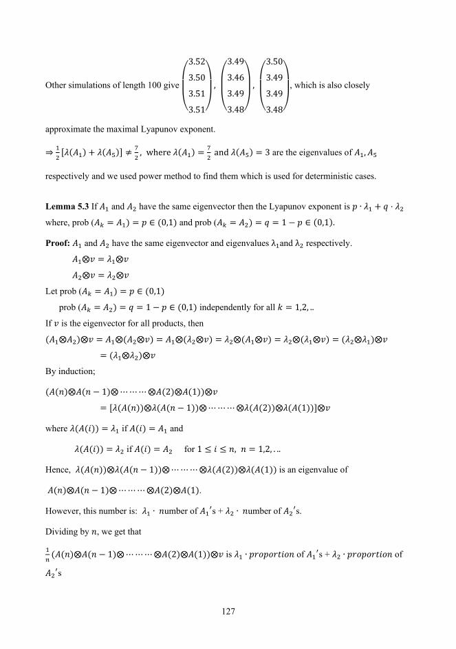
127

Other simulations of length 100 give

⎝

⎜⎛

3.52

3.50

3.51

3.51⎠

⎟⎞

,

⎝

⎜⎛

3.49

3.46

3.49

3.48⎠

⎟⎞

,

⎝

⎜⎛

3.50

3.49

3.49

3.48⎠

⎟⎞

, which is also closely

approximate the maximal Lyapunov exponent.

⇒ 12

[𝜆𝜆(𝐴𝐴1) + 𝜆𝜆(𝐴𝐴5)] ≠ 72

, where 𝜆𝜆(𝐴𝐴1) = 72

and 𝜆𝜆(𝐴𝐴5) = 3 are the eigenvalues of 𝐴𝐴1,𝐴𝐴5

respectively and we used power method to find them which is used for deterministic cases.

Lemma 5.3 If 𝐴𝐴1 and 𝐴𝐴2 have the same eigenvector then the Lyapunov exponent is 𝑝𝑝 ∙ 𝜆𝜆1 + 𝑞𝑞 ⋅ 𝜆𝜆2

where, prob (𝐴𝐴𝑘𝑘 = 𝐴𝐴1) = 𝑝𝑝 ∈ (0,1) and prob (𝐴𝐴𝑘𝑘 = 𝐴𝐴2) = 𝑞𝑞 = 1 − 𝑝𝑝 ∈ (0,1).

Proof: 𝐴𝐴1 and 𝐴𝐴2 have the same eigenvector and eigenvalues λ1and λ2 respectively.

𝐴𝐴1⨂𝑣𝑣 = 𝜆𝜆1⨂𝑣𝑣

𝐴𝐴2⨂𝑣𝑣 = 𝜆𝜆2⨂𝑣𝑣

Let prob (𝐴𝐴𝑘𝑘 = 𝐴𝐴1) = 𝑝𝑝 ∈ (0,1)

prob (𝐴𝐴𝑘𝑘 = 𝐴𝐴2) = 𝑞𝑞 = 1 − 𝑝𝑝 ∈ (0,1) independently for all 𝑘𝑘 = 1,2, ..

If 𝑣𝑣 is the eigenvector for all products, then

(𝐴𝐴1⨂𝐴𝐴2)⨂𝑣𝑣 = 𝐴𝐴1⨂(𝐴𝐴2⨂𝑣𝑣) = 𝐴𝐴1⨂(𝜆𝜆2⨂𝑣𝑣) = 𝜆𝜆2⨂(𝐴𝐴1⨂𝑣𝑣) = 𝜆𝜆2⨂(𝜆𝜆1⨂𝑣𝑣) = (𝜆𝜆2⨂𝜆𝜆1)⨂𝑣𝑣

= (𝜆𝜆1⨂𝜆𝜆2)⨂𝑣𝑣

By induction;

(𝐴𝐴(𝑛𝑛)⨂𝐴𝐴(𝑛𝑛 − 1)⨂⋯⋯⋯⨂𝐴𝐴(2)⨂𝐴𝐴(1))⨂𝑣𝑣

= [𝜆𝜆(𝐴𝐴(𝑛𝑛))⨂𝜆𝜆(𝐴𝐴(𝑛𝑛 − 1))⨂⋯⋯⋯⨂𝜆𝜆(𝐴𝐴(2))⨂𝜆𝜆(𝐴𝐴(1))]⨂𝑣𝑣

where 𝜆𝜆(𝐴𝐴(𝑖𝑖)) = 𝜆𝜆1 if 𝐴𝐴(𝑖𝑖) = 𝐴𝐴1 and

𝜆𝜆(𝐴𝐴(𝑖𝑖)) = 𝜆𝜆2 if 𝐴𝐴(𝑖𝑖) = 𝐴𝐴2 for 1 ≤ 𝑖𝑖 ≤ 𝑛𝑛, 𝑛𝑛 = 1,2, . ..

Hence, 𝜆𝜆(𝐴𝐴(𝑛𝑛))⨂𝜆𝜆(𝐴𝐴(𝑛𝑛 − 1))⨂⋯⋯⋯⨂𝜆𝜆(𝐴𝐴(2))⨂𝜆𝜆(𝐴𝐴(1)) is an eigenvalue of

𝐴𝐴(𝑛𝑛)⨂𝐴𝐴(𝑛𝑛 − 1)⨂⋯⋯⋯⨂𝐴𝐴(2)⨂𝐴𝐴(1).

However, this number is: 𝜆𝜆1 ∙ 𝑛𝑛umber of 𝐴𝐴1′s + 𝜆𝜆2 ∙ 𝑛𝑛umber of 𝐴𝐴2′s.

Dividing by 𝑛𝑛, we get that

1𝑛𝑛

(𝐴𝐴(𝑛𝑛)⨂𝐴𝐴(𝑛𝑛 − 1)⨂⋯⋯⋯⨂𝐴𝐴(2)⨂𝐴𝐴(1))⨂𝑣𝑣 is 𝜆𝜆1 ∙ 𝑝𝑝𝑟𝑟𝑑𝑑𝑝𝑝𝑑𝑑𝑟𝑟𝑡𝑡𝑖𝑖𝑑𝑑𝑛𝑛 of 𝐴𝐴1′s + 𝜆𝜆2 ∙ 𝑝𝑝𝑟𝑟𝑑𝑑𝑝𝑝𝑑𝑑𝑟𝑟𝑡𝑡𝑖𝑖𝑑𝑑𝑛𝑛 of

𝐴𝐴2′s

128

By the law of large numbers, the 𝑝𝑝𝑟𝑟𝑑𝑑𝑝𝑝𝑑𝑑𝑟𝑟𝑡𝑡𝑖𝑖𝑑𝑑𝑛𝑛 of 𝐴𝐴1′𝑠𝑠 → 𝑝𝑝 and

𝑝𝑝𝑟𝑟𝑑𝑑𝑝𝑝𝑑𝑑𝑟𝑟𝑡𝑡𝑖𝑖𝑑𝑑𝑛𝑛 of 𝐴𝐴2′𝑠𝑠 → 𝑞𝑞 = 1 − 𝑝𝑝

∴ The Lyapunov exponent is 𝒑𝒑 ∙ 𝝀𝝀𝟏𝟏 + 𝒒𝒒 ⋅ 𝝀𝝀𝟐𝟐 ∎

Example 5.8 Let 𝐴𝐴1 =

⎝

⎜⎛

2

1

𝜀𝜀

𝜀𝜀

6

𝜀𝜀

5

5

𝜀𝜀

−1

−2

−2

−3

𝜀𝜀

𝜀𝜀

𝜀𝜀 ⎠

⎟⎞⟹ 𝜆𝜆(𝐴𝐴1) = 7

2, and 𝑣𝑣(𝐴𝐴1) = (0 −2.5 −1 −2)𝑇𝑇

Let 𝐴𝐴2 =

⎝

⎜⎛

2.5

1.5

𝜀𝜀

𝜀𝜀

6.5

𝜀𝜀

5.5

4.5

𝜀𝜀

−0.5

−0.5

−1.5

−2.5

𝜀𝜀

𝜀𝜀

𝜀𝜀 ⎠

⎟⎞⟹ 𝜆𝜆(𝐴𝐴2) = 4, and 𝑣𝑣(𝐴𝐴2) = (0 −2.5 −1 −2)𝑇𝑇

The Lyapunov exponent can be found by using the Lemma 5.3.

Note that: 12

[𝜆𝜆(𝐴𝐴1) + 𝜆𝜆(𝐴𝐴2)] = 3.75, where 𝜆𝜆(𝐴𝐴1) = 72

and 𝜆𝜆(𝐴𝐴2) = 4.

Because of 𝑥𝑥(𝑘𝑘 + 1) = 𝐴𝐴(𝑘𝑘) ⊗𝑥𝑥(𝑘𝑘), with 𝐴𝐴(𝑘𝑘) = 𝐴𝐴1 with probability 0.5 and 𝐴𝐴(𝑘𝑘) = 𝐴𝐴2 with

probability 0.5, the matrices 𝐴𝐴1,𝐴𝐴2 are taken to be the stochastic perturbation of the original matrix𝐴𝐴.

i. e.𝐴𝐴𝑡𝑡𝑒𝑒𝑟𝑟𝑡𝑡 = 𝐴𝐴1 or 𝐴𝐴2 .

𝐴𝐴 = maxmult (𝐴𝐴𝑡𝑡𝑒𝑒𝑟𝑟𝑡𝑡 , 𝐼𝐼) for the first iteration where 𝐼𝐼 is the identity matrix.

Thus, 𝐴𝐴 = 𝐴𝐴(𝑠𝑠𝑡𝑡𝑜𝑜𝑡𝑡 𝑖𝑖𝑡𝑡𝑒𝑒𝑟𝑟) 𝐴𝐴(𝑠𝑠𝑡𝑡𝑜𝑜𝑡𝑡 𝑖𝑖𝑡𝑡𝑒𝑒𝑟𝑟−1)⋯⋯⋯⋯⋯⋯⋯⋯⋯⋯⋯⋯⋯⋯⋯⋯⋯⋯⋯𝐴𝐴(3)𝐴𝐴(2)𝐴𝐴(1)

and 𝑥𝑥𝑘𝑘 = 𝐴𝐴⊗ 𝑥𝑥0.

If we have taken, 𝑘𝑘 = 200, then

𝐴𝐴= 𝐴𝐴(200)𝐴𝐴(199)⋯⋯⋯𝐴𝐴(3)𝐴𝐴(2)𝐴𝐴(1)

⇒ 𝐴𝐴 =

⎝

⎜⎛

747.5

746.5

746.5

746.5

751.5

747.5

750.5

750.5

745.5

744.5

744.5

744.5

742.5

738.5

741.5

741.5⎠

⎟⎞

𝑥𝑥200 = 𝐴𝐴⊗ 𝑥𝑥0 =

⎝

⎜⎛

751.5

747.5

750.5

750.5⎠

⎟⎞

129

∴ 𝑚𝑚200200

=

⎝

⎜⎛

3.7575

3.7375

3.7525

3.7525⎠

⎟⎞

which is close to the maximal Lyapunov exponent which is in this case equal

to 3.75

⇒ 12

[𝜆𝜆(𝐴𝐴1) + 𝜆𝜆(𝐴𝐴5)] = 3.75, where 𝜆𝜆(𝐴𝐴1) = 72

and 𝜆𝜆(𝐴𝐴2) = 4 are the eigenvalues of 𝐴𝐴1,𝐴𝐴2

respectively and we used power method to find them which is used for deterministic cases.

5.3.2 Beyond Irreducible Matrices

We will now drop the obligation that 𝐴𝐴(𝑘𝑘) has a minimal support matrix that is irreducible.To deal

with this case, we assume that the position of finite elements of 𝐴𝐴(𝑘𝑘) is fixed and independent of 𝑘𝑘,

and we decompose 𝐴𝐴(𝑘𝑘) into its irreducible parts. The limit theorem, to be submitted briefly, then

states that the Lyapunov exponent of the overall matrix equals the maximum of the Lyapunov

exponent of its irreducible components [2].

Let 𝐴𝐴(𝑘𝑘):𝑘𝑘 ∈ 𝑁𝑁 be a sequence of matrices in ℝ𝑚𝑚𝑚𝑚𝑚𝑚𝑛𝑛×𝑛𝑛 such that the arc set of the communication

graph of 𝐴𝐴(𝑘𝑘) is independent of k and non-random.

For 𝑖𝑖 ∈ 𝑛𝑛, [𝑖𝑖] denotes the set of vertices of the maximal strongly connected subgraph that contains

node 𝑖𝑖, and denote by 𝜆𝜆[𝑖𝑖] the Lyapunov exponent associated to the matrix obtained by restricting

𝐴𝐴(𝑘𝑘) to the vertices in [𝑖𝑖]. We state the theorem without proof.

Theorem 5.5 [2] Let 𝐴𝐴(𝑘𝑘): 𝑘𝑘 ∈ 𝑁𝑁 be an independent identically distributed sequence of regular and

integrable matrices in ℝ𝑚𝑚𝑚𝑚𝑚𝑚𝑛𝑛×𝑛𝑛 such that the communication graph of 𝐴𝐴(𝑘𝑘) has cyclicity one and is

independent of 𝑘𝑘 and non-random [2]. For any finite integrable initial value 𝑥𝑥0, it holds with

probability one that

lim𝑘𝑘→∞

1𝑘𝑘𝑥𝑥𝑖𝑖(𝑘𝑘; 𝑥𝑥0)

𝑘𝑘min

= lim𝑘𝑘→∞

1𝑘𝑘𝑥𝑥𝑖𝑖(𝑘𝑘; 𝑥𝑥0) = 𝜆𝜆𝑖𝑖

with

𝜆𝜆𝑖𝑖 = ⊕ 𝜆𝜆[𝑖𝑖]𝑖𝑖∈𝜋𝜋∗(𝑖𝑖)

, 𝑗𝑗 ∈ 𝑛𝑛.

130

5.4 State Reduction for Matrices with Dominant Maximal

Cycle

In this Section we describe a method to simplify the calculations in some special cases. The amount

of computational work can be reduced significantly, even in the stochastic case, if the maximal cycle

of the involved matrices dominates the weights of the edges between all other nodes in the graph.

State reduction for matrices in max-plus algebra with dominant maximal cycle mean for special case

(stochastic case) can be described into the following definition and two propositions.

Definition 5.3 Let 𝐴𝐴 and 𝐵𝐵 be two matrices. Suppose 𝐴𝐴 and 𝐵𝐵 have maximum cycles involving

𝑖𝑖1, 𝑖𝑖2,⋯ , 𝑖𝑖𝑘𝑘 only. Further assume that all weights involving other nodes are less than the entries in

the maximal cycles of both 𝐴𝐴 and 𝐵𝐵. We say that 𝐴𝐴 and 𝐵𝐵 have a dominant maximum cycle.

In the sequel we will talk about cycles in the matrices 𝐴𝐴 and 𝐵𝐵 instead of the more correct expressions

cycles in the precedence graphs of the matrices 𝐴𝐴 and 𝐵𝐵.

Proposition 5.1 Let 𝐴𝐴 and 𝐵𝐵 have dominant maximum cycle, so that all elements involving other

nodes are less than the entries in the maximal cycles of both 𝐴𝐴 and 𝐵𝐵. Consider the stochastic case

where the probabilities of 𝐴𝐴 and 𝐵𝐵 are p and 1-p, respectively. Then the Lyapunov exponent of the

system can be obtained by restricting the attention to 𝑖𝑖1, 𝑖𝑖2,⋯ , 𝑖𝑖𝑘𝑘 only.

Proof: Suppose the maximal cycle of the matrices A and B is 𝑖𝑖1, 𝑖𝑖2,⋯ , 𝑖𝑖𝑘𝑘 . Suppose that we

substitute this for another cycle with edges outside of the set 𝑖𝑖1, 𝑖𝑖2,⋯ , 𝑖𝑖𝑘𝑘 . Then necessarily its

weight is decreased because all edges going outside the given set have lower weights than any of the

weights in the maximal cycle.

∎

Proposition 5.2 Let 𝐴𝐴 and 𝐵𝐵 be two matrices and 𝑐𝑐 a scalar. If 𝐴𝐴 and 𝐵𝐵 are replaced by 𝐴𝐴 + 𝑐𝑐 and

𝐵𝐵 + 𝑐𝑐 respectively then the Lyapunov exponent increases by 𝑐𝑐.

Proof: All edges of the matrices A and B are increased by c. Any entry in the product A⨂B is

increased by 2c: ((𝐴𝐴 + 𝑐𝑐) ⨂ (𝐵𝐵 + 𝑐𝑐))𝑖𝑖𝑘𝑘 = max𝑖𝑖 ((𝐴𝐴 + 𝑐𝑐)𝑖𝑖𝑖𝑖 + (𝐵𝐵 + 𝑐𝑐)𝑖𝑖𝑘𝑘) = max𝑖𝑖 (𝐴𝐴𝑖𝑖𝑖𝑖 + 𝑐𝑐 +

𝐵𝐵𝑖𝑖𝑘𝑘 + 𝑐𝑐) = (𝐴𝐴⨂𝐵𝐵)𝑖𝑖𝑘𝑘 + 2𝑐𝑐.

Similarly, the entries in any product of N factors of A’s and B’s are increased by 𝑁𝑁𝑐𝑐. The mean of all

cycles is thus increased by 𝑐𝑐 and so the Lyapunov exponent, too, is increased by 𝑐𝑐.

∎

131

Example 5.9 Let 𝐴𝐴 and 𝐵𝐵 are two matrices with prob (𝐴𝐴) = 12 and prob (𝐵𝐵) = 1

2, where

𝐴𝐴 =

⎝

⎜⎛

2

1

0

0

6

𝜀𝜀

1

2

1

2

−1

2

2

0

−1

0 ⎠

⎟⎞

has eigenvalue 𝜆𝜆(𝐴𝐴) = 3.5

𝐴𝐴 − 3 =

⎝

⎜⎛

−1

−2

−3

−3

3

𝜀𝜀

−2

−1

−2

−1

−4

−1

−1

−3

−4

−3⎠

⎟⎞

𝜆𝜆(𝐴𝐴 − 3) = 0.5 = 𝜆𝜆(𝐴𝐴) − 3

Example 5.10 Let 𝐴𝐴 =

⎝

⎜⎛

2

1

0

0

6

𝜀𝜀

0

−1

0

0

−1

0

0

0

−1

0 ⎠

⎟⎞

and the eigenvalue 𝜆𝜆(𝐴𝐴) = 3.5

𝐴𝐴𝑟𝑟𝑒𝑒𝑠𝑠𝑡𝑡𝑟𝑟. = 2 61 𝜀𝜀 involves nodes 1 and 2 only. The eigenvalue of 𝐴𝐴𝑟𝑟𝑒𝑒𝑠𝑠𝑡𝑡𝑟𝑟. = 𝜆𝜆(𝐴𝐴) = 3.5

𝐴𝐴 − 3 =

⎝

⎜⎛

−1

−2

−3

−3

3

𝜀𝜀

−3

−4

−3

−3

−4

−3

−3

−3

−4

−3⎠

⎟⎞

has eigenvalue 0.5= 𝜆𝜆(𝐴𝐴) − 3

𝐴𝐴𝑟𝑟𝑒𝑒𝑠𝑠𝑡𝑡𝑟𝑟. − 3 = −1 3−2 𝜀𝜀

Let 𝐵𝐵 =

⎝

⎜⎛

2

1

0

0

5

𝜀𝜀

0

0

0

0

0

0

0

0

0

0⎠

⎟⎞

has eigenvalue 𝜆𝜆(𝐵𝐵) = 3

132

𝐵𝐵 − 3 =

⎝

⎜⎛

−1

−2

−3

−3

2

𝜀𝜀

−3

−3

−3

−3

−3

−3

−3

−3

−3

−3⎠

⎟⎞

has eigenvalue 0 = 𝜆𝜆(𝐵𝐵)− 3

𝐵𝐵𝑟𝑟𝑒𝑒𝑠𝑠𝑡𝑡𝑟𝑟. − 3 = −1 2−2 𝜀𝜀

To show that by using the graph theory:

The graph of the matrix A (see Figure 5.9) shows that the maximum cycle mean is 𝐴𝐴12+𝐴𝐴212

= 6+12

=

3.5

Figure 5.11: The precedence graph of the matrix 𝐴𝐴

And the graph of the 𝐴𝐴𝑟𝑟𝑒𝑒𝑠𝑠𝑡𝑡𝑟𝑟. = 2 61 𝜀𝜀 (see Figure 5.10) which is also includes the maximum cycle

mean:

Figure 5.12: The precedence graph of the matrix 𝐴𝐴𝑟𝑟𝑒𝑒𝑠𝑠𝑡𝑡𝑟𝑟.

In the next example we going to show how dimension reduction can be done by uniformly dominant

circuit.

Example 5.11 Let 𝐴𝐴 and 𝐵𝐵 are two matrices with prob (𝐴𝐴) = 12 and prob (𝐵𝐵) = 1

2, where

𝐴𝐴 =

⎝

⎜⎛

𝜀𝜀

2

0

−1

0

𝜀𝜀

0

0

𝜀𝜀

𝜀𝜀

𝜀𝜀

0

𝜀𝜀

−1

𝜀𝜀

𝜀𝜀 ⎠

⎟⎞

has eigenvalue 𝜆𝜆(𝐴𝐴) = 1

133

Figure 5.13: The precedence graph of the matrix 𝐴𝐴

If we reduce the dimensions by reduction uniformly dominant circuit, then we get

𝐴𝐴1 = 𝜀𝜀 02 𝜀𝜀 which it has the same eigenvalue

Figure 5.14: The precedence graph of the matrix 𝐴𝐴1

And for the matrix 𝐵𝐵 =

⎝

⎜⎛

−1

3

𝜀𝜀

0

2

−2

0

0

𝜀𝜀

𝜀𝜀

0

0

−1

𝜀𝜀

0

0 ⎠

⎟⎞

which has the eigenvalue 𝜆𝜆(𝐵𝐵) = 2.5

Figure 5.15: The precedence graph of the matrix 𝐵𝐵

If we reduce the dimensions by reduction uniformly dominant circuit, then we get

𝐵𝐵1 = −1 23 −2

134

Figure 5.16: The precedence graph of the matrix 𝐵𝐵1

Next, we will show how to use the dimension reduction to compute the Lyapunov exponent more

easily. We learn from ([2] Chapter 11 pp. 175) that the stochastic matrix products

give rise to a Markov chain on the set of directions of vectors in Rmax𝑑𝑑 . The Lyapunov exponent can

be calculated by using the stationary probability distribution 𝜋𝜋 of the Markov chain on directions: the

exponent is the average growth (with respect to π) under multiplication by A and B (independently of

each other, with the given probabilities p and 1-p).

The direction of a vector u is simply u (max plus −) divided by its length.

Let 𝑢𝑢 = (𝑢𝑢1 𝑢𝑢2 . . . . 𝑢𝑢𝑘𝑘)𝑇𝑇. Its length is taken to be the (max plus-sum or) maximum entry max𝑖𝑖 𝑢𝑢𝑖𝑖,

1 ≤ 𝑖𝑖 ≤ 𝑘𝑘, and its direction is then the vector 𝑢𝑢 − max𝑖𝑖 𝑢𝑢𝑖𝑖 which obviously has length 0. In our

examples below, the sign ~ denotes equal direction of two vectors.

The case of norming by “𝑠𝑠𝑢𝑢𝑚𝑚 = max” is show in the following example.

Example 5.12 Let 𝐶𝐶 and 𝐷𝐷 are two matrices with prob (𝐶𝐶) = 12 and prob (𝐷𝐷) = 1

2, where

𝐶𝐶 = 1 13 0 , 𝐷𝐷 = 1 3

0 2 and 𝜆𝜆(𝐶𝐶) = 𝜆𝜆(𝐷𝐷) = 2 . It turns out that the process generates a Markov

chain on three directions:

𝐶𝐶⨂00 = 1

3~ −20

𝐶𝐶⨂−20 = 1

1~ 00

𝐷𝐷⨂00 = 3

2~ 0−1

𝐷𝐷⨂ 0−1 = 2

1~ 0−1

𝐷𝐷⨂−20 = 3

2~ 0−1

𝐶𝐶⨂ 0−1 = 1

3~ −20

we know that; 𝑃𝑃(𝐶𝐶) = 𝑃𝑃(𝐷𝐷) = 12

Thus:

135

00 −2

0 0−1

00 0 1

2 1

2

−20 1

2 0 1

2

0−1 0 1

2 1

2

Figure 5.17: Markov chain with transition probabilities

Thus, the stationary distribution for the Markov chain is 𝜋𝜋 = 1613

12

The average growth of maximal Lyapunov exponent is in this case equal to 6+8+1512

= 2912

= 2.41667

where 12

[𝜆𝜆(𝐶𝐶) + 𝜆𝜆(𝐷𝐷)] = 42

= 2.

In the case of Example 5.11. the average growth of maximal Lyapunov exponent is equal to 180102

=

1.7647, while 12

[𝜆𝜆(𝐴𝐴) + 𝜆𝜆(𝐵𝐵)] = 3.52

= 1.75, where 𝜆𝜆(𝐴𝐴) = 2.5 and 𝜆𝜆(𝐵𝐵) = 1 are the eigenvalues

of 𝐴𝐴,𝐵𝐵 respectively.

Here the Markov chain on directions is 00 , −2

0 , 01 and −1

0 and the stationary distribution

π = 1814

14 3

8.

Note. If the dominant cycle consists of one element only, then the Lyapunov exponent is simply

12

[𝜆𝜆(𝐴𝐴) + 𝜆𝜆(𝐵𝐵)].

136

Example 5.13 In 4.4.2, M2. The production of D and E using only one of the units for D, during the

filling stage and this has been formulated by using a max-plus model and after introduction of

numerical values from Table 4.1, the A-matrix of the system becomes

𝐴𝐴 = 10 4

14 8, the eigenvalue 𝜆𝜆(𝐴𝐴) = 10

Now take

𝐵𝐵 = 10 1214 16 which it has the eigenvalue 16.

It turns out that the process generates a Markov chain on one direction:

𝐴𝐴⨂00 = 10

14~ −40

𝐴𝐴⨂−40 = 6

10~ −40

𝐵𝐵⨂00 = 12

16~ −40

𝐵𝐵⨂−40 = 12

16~ −40

Suppose that; 𝑃𝑃(𝐴𝐴) = 𝑃𝑃(𝐵𝐵) = 12 . The Markov chain is trivial, on only one direction.

This is a case where both matrices have the same eigenvector. In other words, we can immediately

use Lemma 5.3. Thus, the Lyapunov exponent is 13.

We can make the matrix 𝐴𝐴 stochastic by changing, for instance, 4 to 6 and 14 to 16, in this case, the

A-matrix becomes;

𝐴𝐴 = 10 6

16 8 which it has the eigenvalue 11.

It turns out that the process generates a Markov chain on one direction:

𝐴𝐴⨂00 = 10

16~ −60

𝐴𝐴⨂−60 = 6

10~ −40

𝐴𝐴⨂−40 = 6

12~ −60

𝐵𝐵⨂00 = 12

16~ −40

𝐵𝐵⨂−40 = 12

16~ −40

𝐵𝐵⨂−60 = 12

16~ −40

137

Figure 5.18: Markov chain with transition probabilities

Here the Markov chain on directions is −60 and −4

0 and the stationary distribution

π = 13

23 .

The average growth of maximal Lyapunov exponent is in this case equal to 13.67 where 12

[𝜆𝜆(𝐴𝐴) + 𝜆𝜆(𝐵𝐵)] = 11+162

= 13.5

138

139

Chapter 6

General Conclusion The aim of this thesis was to provide an introductory text on max-plus algebra and to present results

on advanced topics and, in particular, how it is useful in applications. An overview of the basic notions

of the max-plus algebra and max-plus linear discrete event systems (DES) was presented. The basic

operations, definitions, theorems, and properties of the max-plus algebra were introduced. The main

feature of max-plus algebra is that addition is replaced by max, and multiplication is replaced by

addition. This is useful especially for modeling, simulating and optimizing nonlinear scheduling

problems using linear algebra methods.

Chapters 1-2 aimed to be a guide through basic max-plus algebra, where Chapter 1 presented simple

introduction of max-plus algebra properties, matrices and graphs. Chapter 2 implemented the solution

of linear systems such as 𝐴𝐴⨂𝑥𝑥 = 𝑏𝑏, linear independence and dependence, and presented the max-

plus eigenproblem in detail. Efficient methods for finding all eigenvalues and describing all

eigenvectors for any square matrix over ℝmax = ℝ⋃−∞, with all the necessary proofs, were

presented. The modeling of production systems using max-plus DES was discussed, and two

examples were also presented. Analogue to characteristic equation and the Cayley–Hamilton theorem

in max-plus algebra were introduced.

Chapter 3 described how a max-plus model for a train system can be constructed. Meeting conditions

caused by having only a single track, and other physical constrains, have been modeled. A state update

equation of the form 𝑥𝑥(𝑘𝑘) = 𝐴𝐴⨂𝑥𝑥(𝑘𝑘 − 1) is desirable, which was made possible by using cross-

substitutions and extending the state space with delayed states. Static and dynamic delay sensitivity

of the network has been analyzed by modifying the 𝐴𝐴-matrix and using eigenvalue calculations. The

obtained results were compared to recovery matrix-based calculations found in the literature. A

recovery matrix for the chosen extended state space becomes large and contains even irrelevant

information. Guidelines for finding and interpreting the relevant information from the recovery matrix

have been discussed. Max-plus formalism was used throughout this chapter.

140

The main contribution of this thesis is found in Chapter 4, where it was described how a max-plus

model for a manufacturing system can be constructed, and an optimal schedule was found without

optimization. The scheduling of production systems consisting of many stages and different units was

considered, where some of the units were used for multiple production stages. If a production unit is

used for different stages, cleaning is needed in between, while no cleaning is needed between stages

of the same type. The obtained state update equation was in this case also rewritten in the form 𝑥𝑥(𝑘𝑘) =

𝐴𝐴⨂𝑥𝑥(𝑘𝑘 − 1) using several cross-substitutions, and extension of the state space with delayed states.

Structural decisions, such as using a unit for different tasks, were found difficult to formulate in max-

plus algebra. Three possible operation modes with the structure fixed was identified and modeled

separately using max plus. The central driving factor for structural switches was durability

constraints, which were present in the production. Thus, only a part of the schedule was obtained by

solving eigenvalue problems of the max-plus model, the structural decisions were made on the basis

of a few alternative schedules obtained using max-plus. This was based on the finding that structural

switches should be postponed as late as possible, so the criterion used was to do the switch one step

before the step that was the first that violated at least one durability constraint. Using this strategy, an

optimal schedule was obtained without any optimization.

Chapter 5 provides a thorough review and explanation of the theory of stochastic max-plus linear

systems, which has seen fast developments in the last two decades. Ergodic theory for stochastic max-

plus linear systems has been presented where the common approaches were discussed. Examples of

stochastic max-plus linear systems production system were presented, and the Lyapunov exponent

was found by using simulation. Connections to Petri nets was also discussed in this chapter.

141

References [1] F. Baccelli, G. Cohen, G.L. Olsder and J.P Quadrat (1992), Synchronization and Linearity,

Wiley, New York.

[2] Heidergott B, Olsder GJ, van der Woude J (2006) Max Plus at Work: Modeling and Analysis of

Synchronized Systems. A Course on Max-Plus Algebra and its Application. Princeton University

Press, Princeton

[3] De Schutter B, van den Boom TJJ (2008). Max-plus algebra and max-plus linear discrete event

systems: An introduction. In Proceedings of WODES 2008, 9th International Workshop on

Discrete Event Systems, IEEE.

[4] M Akian R. Bapat, and S. Gaubert (1998), Asymptotics of the Perron eigenvalue and eigenvector

using max-algebra, C. R. Acad. Sci. Paris, Seire 1, Vol. 327: 927-932.

[5] M.Akian, R. Bapat, S. Gaubert (2007), Max-plus algebras, Chapter 25 in the Handbook of

Linear Algebra, L. Hogben, R. Brualdi, A. Greenbaum, and R. Mathias (editors), Discrete

Mathematics and Its Applications, 39.

[6] J.G. Braker and G.J. Olsder (1993), The power algorithm in the max algebra, Linear Algebra

and its Applications, Vol. 182: 67-89.

[7] Bart De Schutter, Bart De Moor (1997), A note on the Characteristics Equation in the Max-Plus

Algebra, Linear Algebra and its Applications, Vol. 261: 237-250.

[8] de Shutter B (2000), On the ultimate behavior of the sequence of consecutive powers of a matrix

in the max-plus algebra, Linear Algebra and its Applications, Vol. 307: 103-117.

[9] R.A. Cuninghame-Green and P Butkovic (2004), Bases in max-algebra, Linear Algebra and its

Applications, Vol. 389: 107-120.

[10] B.De Schutter B (1996), Max-algebraic system theory for discrete event systems, Ph.D.

dissertation, Faculty of Applied Sciences, K.U. Leuven, Leuven, Belgium.

[11] G. Olsder and C. Roos (1988), Cramer and Cayley-Hamilton in the max algebra, Linear Algebra

and Its Applications, Vol. 101: 87-108.

[12] Elsner L. and P. van den Driessche (1999), On the power method in max algebra, Linear Algebra

and its Applications 302-303 (1999) 17-32

142

[13] Braker JG and Olsder GJ (1993), The power algorithm in the max algebra, Linear Algebra And

its Applications, Vol.182: 67-89.

[14] R.E. Burkard and P. Butkovic (2003), Finding all essential terms of a characteristic

maxpolynomial, Discrete Applied Mathematics, Vol. 130: 367-380

[15] R.E.Burkard and E.Çela (1999), Linear Assignment Problems and Extensions, in Handbook of

Combinatorial Optimization (P.M.Pardalos and D.-Z.Du, Eds.), Supplement Volume A, Kluwer

Academic Publishers.

[16] P.Butkovic (2003), Max-algebra: the linear algebra of combinatorics, Linear Algebra and

Applications, Vol. 367: 313-335.

[17] P.Butkovic and H.Schneider (2005), Applications of max-algebra to diagonal scaling of

matrices, Electronic Journal of Linear Algebra, Vol.13: 262-273.

[18] P.Butkovic, H.Schneider and S.Sergeev (2005), Generators, Extremals and Bases of Max Cones,

Linear Algebra and Its Applications, Vol. 421: 394-406.

[19] P.Butkovic (2008), Finding a bounded mixed-integer solution to a system of dual inequalities,

Operations Research Letters, Vol. 36: 623-627.

[20] P.Butkovic (2010), Max-linear Systems: Theory and Algorithms, Springer, Birmingham.

[21] B.A.Carré (1971), An algebra for network routing problems, IMA Journal of Applied

Mathematics, Vol 7: 273–294.

[22] W.Chen, X.Qi and S.Deng (1990), The Eigen problem and period analysis of the discrete event

systems, System Science and Complexity: English Edition, 1990, Issue 3: 243-260.

[23] Heidergott, Bernd F (2007), Max-Plus Linear Stochastic Systems and Perturbation Analysis,

Springer, New York.

[24] Van den Boom TJJ, De Schutter B (2004). Modeling and control of railway networks.

Proceedings of the 2004 American Control Conference. Vol. 6. IEEE.

[25] Goverde RMP (2007). Railway timetable stability analysis using max-plus system theory,

Transportation Research Part B: Methodological, Vol. 41: 179-201.

[26] Goverde RMP (2010). A delay propagation algorithm for large-scale railway traffic networks,

Transportation Research Part C: Emerging Technologies, Vol.18: 269-287.

[27] De Schutter B, van den Boom TJJ, Hegyi A (2002). A model predictive control approach for

recovery from delays in railway systems. Transportation Research Record, Vol. 1793: 15-20.

[28] D'Ariano A, Pacciarelli D, Pranzo M (2007). A branch and bound algorithm for scheduling trains

in a railway network. European Journal of Operational Research 183(2): 643-657.

143

[29] Corman F, D'Ariano A, Pacciarelli D, Pranzo M (2012). Bi-objective conflict detection and

resolution in railway traffic management. Transportation Research Part C: Emerging

Technologies Vol. 20: 79-94.

[30] Van den Boom TJJ, Kersbergen B, De Schutter B (2012). Structured modeling, analysis, and

control of complex railway operations. In: Proceedings of the 51st IEEE Conference on Decision

and Control, Maui, Hawaii, pp. 7366-7371.

[31] Kecman P, Corman F, D'Ariano A, Goverde RM (2013). Rescheduling models for railway traffic

management in large-scale networks. Public Transport Vol. 5(1-2):95-123.

[32] Timetables for long-distance trains between Turku and Helsinki, available on

https://www.vr.fi/cs/vr/en/long-distance_timetables (accessed sixth of March 2014).

[33] Björkqvist J, Roslöf J, Rönnback R, Westerlund T, (2002). Evaluation of an Iterative

Mathematical Optimization Approach for Industrial Size Batch Scheduling. Fifth Italian

conference on chemical and process engineering.

[34] Giffler, B. and Thompson, GL. (1960). Algorithms for Solving Production-Scheduling

Problems. Operations Research, 8: 487-503.

[35] Mutsaers M, Özkan L, Backx T, (2012). Scheduling of energy flows for parallel batch processes

using max-plus systems. Eighth IFAC Symposium on Advanced Control of Chemical Processes,

Singapore, Vol. 45: 614-619.

[36] K. Zimmermann (1976), Extremální algebra, Výzkumná publikace Ekonomicko–matematické

laboratoˇreprˇi Ekonomickém ústaveˇ Cˇ SAV, 46, Praha, (in Czech).

[37] Al bermanei H, Böling JM, and Högnäs G (2016), Modeling and simulation of train networks

using max-plus algebra. The 9th EUROSIM Congress on Modelling and Simulation EUROSIM

2016, Oulu, Finland, DOI: 10.3384/ecp17142: pp. 612-618.

[38] Al bermanei H, Böling JM, and Högnäs G (2017). Modeling and scheduling of production

system by using max-plus algebra. International Conference on Innovative Technologies (In-

Tech 2017), Ljubljana, Slovenia. Awarded for science technology transfer at the conference, Vol.

4, SI-1291: pp.37-40.

[39] Gondran M, Minoux M (1984) Linear algebra of dioïds: a survey of recent results. Annals of

Discrete Mathematics, Vol. 19:147-164.

[40] J.R.S. Dias, C.A. Maia & V.F. Lucena Jr. (2015). Synchronising operations on productive

systems modelled by timed event graphs, International Journal of Production Research,

DOI:10.1080/00207543.2015.1041573

Hazem Al Bermanei

Applications of Max-Plus Algebra to Scheduling

Hazem

Al B

ermanei /

/ Ap

plicatio

ns of M

ax-Plus Alg

ebra to

Scheduling

// 2

02

1

ISBN 978-951-765-983-3