applications of linear parameter...
TRANSCRIPT

APPLICATIONS OF LINEAR PARAMETER-VARYING CONTROL FORAEROSPACE SYSTEMS
By
KRISTIN LEE FITZPATRICK
A THESIS PRESENTED TO THE GRADUATE SCHOOLOF THE UNIVERSITY OF FLORIDA IN PARTIAL FULFILLMENT
OF THE REQUIREMENTS FOR THE DEGREE OFMASTER OF SCIENCE
UNIVERSITY OF FLORIDA
2003

TABLE OF CONTENTSpage
LIST OF TABLES . . . . . . . . . . . . . . . . . . . . . . . . . . . . . . . . . . . iv
LIST OF FIGURES . . . . . . . . . . . . . . . . . . . . . . . . . . . . . . . . . . . v
ABSTRACT . . . . . . . . . . . . . . . . . . . . . . . . . . . . . . . . . . . . . . . vii
CHAPTER
1 INTRODUCTION . . . . . . . . . . . . . . . . . . . . . . . . . . . . . . . . 1
1.1 Overview . . . . . . . . . . . . . . . . . . . . . . . . . . . . . . . . . 11.2 Background . . . . . . . . . . . . . . . . . . . . . . . . . . . . . . . . 2
2 LINEAR PARAMETER-VARYING CONTROL THEORY . . . . . . . . . . 5
3 LINEAR PARAMETER-VARYING CONTROL FOR AN F/A-18 . . . . . . . 10
3.1 Problem Statement . . . . . . . . . . . . . . . . . . . . . . . . . . . . 103.2 Open-loop Dynamics . . . . . . . . . . . . . . . . . . . . . . . . . . . 123.3 Control Objectives . . . . . . . . . . . . . . . . . . . . . . . . . . . . 143.4 Synthesis . . . . . . . . . . . . . . . . . . . . . . . . . . . . . . . . . 153.5 Simulation . . . . . . . . . . . . . . . . . . . . . . . . . . . . . . . . . 173.6 Conclusion . . . . . . . . . . . . . . . . . . . . . . . . . . . . . . . . . 20
4 LINEAR PARAMETER-VARYING CONTROL FOR A HYPERSONICAIRCRAFT . . . . . . . . . . . . . . . . . . . . . . . . . . . . . . . . . . . 22
4.1 Problem Statement . . . . . . . . . . . . . . . . . . . . . . . . . . . . 224.2 Generic Hypersonic Vehicle . . . . . . . . . . . . . . . . . . . . . . . 254.3 Hypersonic Model . . . . . . . . . . . . . . . . . . . . . . . . . . . . . 264.4 Linear Parameter-Varying System . . . . . . . . . . . . . . . . . . . . 274.5 Control Design . . . . . . . . . . . . . . . . . . . . . . . . . . . . . . 304.6 Simulation . . . . . . . . . . . . . . . . . . . . . . . . . . . . . . . . . 33
4.6.1 Open-Loop Simulation . . . . . . . . . . . . . . . . . . . . . . 334.6.2 Closed-Loop Simulation . . . . . . . . . . . . . . . . . . . . . 35
4.7 Conclusion . . . . . . . . . . . . . . . . . . . . . . . . . . . . . . . . . 38
5 LINEAR PARAMETER-VARYING CONTROL FOR A DRIVEN CAVITY . 39
5.1 Problem Statement . . . . . . . . . . . . . . . . . . . . . . . . . . . . 395.2 Background . . . . . . . . . . . . . . . . . . . . . . . . . . . . . . . . 40
ii
5.3 Driven Cavity Geometry . . . . . . . . . . . . . . . . . . . . . . . . . 415.4 Governing Equations of Motion . . . . . . . . . . . . . . . . . . . . . 425.5 Reduced-Order Linear Dynamics . . . . . . . . . . . . . . . . . . . . . 445.6 Creeping Flow in a Driven Cavity . . . . . . . . . . . . . . . . . . . . 475.7 Excitation Phase Differential . . . . . . . . . . . . . . . . . . . . . . . 495.8 Control Design . . . . . . . . . . . . . . . . . . . . . . . . . . . . . . 50
5.8.1 Control Objectives . . . . . . . . . . . . . . . . . . . . . . . . . 505.8.2 Synthesis . . . . . . . . . . . . . . . . . . . . . . . . . . . . . . 53
5.9 Simulation . . . . . . . . . . . . . . . . . . . . . . . . . . . . . . . . . 545.9.1 Open-Loop Simulation . . . . . . . . . . . . . . . . . . . . . . 545.9.2 Reduced-Order Closed-Loop Simulation . . . . . . . . . . . . . 575.9.3 Full-Order Closed-Loop Simulation . . . . . . . . . . . . . . . 60
5.10 Conclusion . . . . . . . . . . . . . . . . . . . . . . . . . . . . . . . . . 63
6 CONCLUSION . . . . . . . . . . . . . . . . . . . . . . . . . . . . . . . . . . 64
REFERENCES . . . . . . . . . . . . . . . . . . . . . . . . . . . . . . . . . . . . . 65
BIOGRAPHICAL SKETCH . . . . . . . . . . . . . . . . . . . . . . . . . . . . . . 70
iii
LIST OF TABLESTable page
3–1 Original Design Points . . . . . . . . . . . . . . . . . . . . . . . . . . . . . 12
3–2 Frequency and Damping Ratio of Design and Analysis Models . . . . . . . 14
3–3 Frequencies and Damping Ratios of the Target Model . . . . . . . . . . . . 16
3–4 Induced Norms of Closed-Loop System . . . . . . . . . . . . . . . . . . . 17
3–5 Numerical Results . . . . . . . . . . . . . . . . . . . . . . . . . . . . . . . 19
4–1 Model Dimensions and Flight Conditions . . . . . . . . . . . . . . . . . . 27
4–2 Modes of the Hypersonic Model . . . . . . . . . . . . . . . . . . . . . . . 30
4–3 Modes of the Target Model . . . . . . . . . . . . . . . . . . . . . . . . . . 32
4–4 Open-Loop Synthesis Norms . . . . . . . . . . . . . . . . . . . . . . . . . 33
4–5 Point Design Norms . . . . . . . . . . . . . . . . . . . . . . . . . . . . . . 33
5–1 Induced Norms of Closed-Loop System . . . . . . . . . . . . . . . . . . . 53
iv

LIST OF FIGURESFigure page
2–1 H∞ Block Diagram (Gain-Scheduled) . . . . . . . . . . . . . . . . . . . . 7
3–1 F/A-18 . . . . . . . . . . . . . . . . . . . . . . . . . . . . . . . . . . . . . 11
3–2 Flight Envelope/Parameter Space . . . . . . . . . . . . . . . . . . . . . . . 12
3–3 Synthesis Block Diagram . . . . . . . . . . . . . . . . . . . . . . . . . . . 15
3–4 Closed-loop Block Diagram . . . . . . . . . . . . . . . . . . . . . . . . . 18
3–5 Pitch Rate for Design Points . . . . . . . . . . . . . . . . . . . . . . . . . 18
3–6 Pitch Rate for Analysis Point . . . . . . . . . . . . . . . . . . . . . . . . . 19
3–7 Controller Elevator Deflection . . . . . . . . . . . . . . . . . . . . . . . . 19
4–1 Inner-Loop/Outer-Loop Design . . . . . . . . . . . . . . . . . . . . . . . . 25
4–2 Simplified Model of a Generic Hypersonic Vehicle . . . . . . . . . . . . . 25
4–3 Synthesis Block Diagram . . . . . . . . . . . . . . . . . . . . . . . . . . . 31
4–4 Open-Loop Transfer Functions . . . . . . . . . . . . . . . . . . . . . . . . 34
4–5 Open-Loop Angle of Attack Result . . . . . . . . . . . . . . . . . . . . . 35
4–6 Input Elevon Deflection . . . . . . . . . . . . . . . . . . . . . . . . . . . . 35
4–7 Closed-loop Design . . . . . . . . . . . . . . . . . . . . . . . . . . . . . . 36
4–8 Closed-Loop Transfer Functions . . . . . . . . . . . . . . . . . . . . . . . 36
4–9 Closed-Loop Angle of Attack Result . . . . . . . . . . . . . . . . . . . . . 37
4–10 Elevon Deflection Command . . . . . . . . . . . . . . . . . . . . . . . . . 38
4–11 Elevon Deflection Rate . . . . . . . . . . . . . . . . . . . . . . . . . . . . 38
5–1 Stokes Driven Cavity Flow Problem . . . . . . . . . . . . . . . . . . . . . 41
5–2 Controller Block Diagram . . . . . . . . . . . . . . . . . . . . . . . . . . 51
5–3 Open-Loop Flow Velocities for Full-Order Model . . . . . . . . . . . . . . 55
v

5–4 Open-Loop Flow Velocities for Reduced-Order Model with 165o PhaseDifferential . . . . . . . . . . . . . . . . . . . . . . . . . . . . . . . . . 56
5–5 Open-Loop Flow Velocities for Reduced-Order Model with 210o PhaseDifferential . . . . . . . . . . . . . . . . . . . . . . . . . . . . . . . . . 56
5–6 Trajectory of Phase Differential . . . . . . . . . . . . . . . . . . . . . . . 56
5–7 Open-Loop Flow Velocities for Reduced-Order Model over a Trajectoryof Phase Differentials . . . . . . . . . . . . . . . . . . . . . . . . . . . . 57
5–8 Closed-loop System . . . . . . . . . . . . . . . . . . . . . . . . . . . . . . 58
5–9 Closed-Loop Flow Velocities for Reduced-Order Model with 165o PhaseDifferential . . . . . . . . . . . . . . . . . . . . . . . . . . . . . . . . . 59
5–10 Closed-Loop Flow Velocities for Reduced-Order Model with 210o PhaseDifferential . . . . . . . . . . . . . . . . . . . . . . . . . . . . . . . . . 59
5–11 Closed-Loop Flow Velocities for Reduced-Order Model over a Trajec-tory of Phase Differentials . . . . . . . . . . . . . . . . . . . . . . . . . 60
5–12 Closed-Loop Flow Velocities for Full-Order Model . . . . . . . . . . . . . 61
5–13 Closed-Loop Flow Velocities for Full-Order Model with Controller As-sociated with 165o Phase Differential . . . . . . . . . . . . . . . . . . . 61
5–14 Closed-Loop Flow Velocities for Full-Order Model with Controller As-sociated with 210o Phase Differential . . . . . . . . . . . . . . . . . . . 62
5–15 Closed-Loop Flow Velocities for Full-Order Model over a Trajectory ofPhase Differentials . . . . . . . . . . . . . . . . . . . . . . . . . . . . . 62
vi

Abstract of Thesis Presented to the Graduate Schoolof the University of Florida in Partial Fulfillment of the
Requirements for the Degree of Master of Science
APPLICATIONS OF LINEAR PARAMETER-VARYING CONTROL FORAEROSPACE SYSTEMS
By
Kristin Lee Fitzpatrick
December 2003
Chair: Richard C. Lind, Jr.Major Department: Mechanical and Aerospace Engineering
Gain-scheduling control has been an engineering practice for decades and can
be described as the linear regulation of a system whose parameters are changed as a
function of varying operating conditions. Several gain-scheduling techniques have been
researched for the control of systems that vary with time-varying parameters. These
techniques create controllers at various points within the parameter space of the system
and use an interpolation law to change controllers as the parameter changes with time.
The process of creating such an interpolation law can be very rigorous and time-
consuming and the resulting controller is not guarnateed to stablize the time-varying
system. The gain-scheduling technique known as linear parameter-varying control,
however, solves a linear matrix inequality convex problem to create a single controller
that has an automatic interpolation law and is guaranteed to stabilize the closed-loop
system. This paper demonstrates the use of this technique to create controllers for three
aerospace systems. The first system is the longitudinal dynamics of the F/A-18, the
second system is the structural dynamics of a hypersonic vehicle and the third system
is the flow dynamics within a driven cavity. Simulations are performed using the linear
vii

parameter-varying controller created for each system to show the usefulness of a linear
parameter-varying framework as a gain-schedule design technique.
viii

CHAPTER 1INTRODUCTION
1.1 Overview
The dynamics of aerospace systems that deal with flight and process control
are affected by variations in the parameters that make up their operating space (i.e.,
altitude, Mach number, temperature). Gain-scheduling techniques are used to create
a controlling scheme that will work throughout the system’s operating space. The
resulting controller will vary based on the same parameters as the system’s plant
model.
The traditional gain-scheduling technique can be broken down into three major
steps. The first step involves separating the operating range into subspaces and creating
a parameterized model of each subspace. In the second step, controllers are created
for each of these models. Finally, in the third step, a scheduling scheme is devised by
linearly interpolating between these regional controllers as the vehicle moves through
its operating range. This technique works well for some systems; however, it does not
guarantee stability and robustness of the closed-loop system. Another disadvantage
of this method is the possibility of a skipping behavior due to the switch between
controllers.
This thesis presents the technique of creating a single gain-scheduled controller
that can be treated as a single entity. This technique achieves gain-scheduling with a
parameter-dependent controller that will work throughout an operating range or flight
envelope. Benefits of this technique are that it removes the need of creating several
controllers for different parameters within an operating domain and removes the need
for the creation of a gain-scheduled control law.
1

2
This study applies this method to three specific aerospace systems. The first
application of this technique is creation of a controller for the F/A-18 longitudinal
axes over a specific flight envelope. The second application is control of the structural
dynamics of a hypersonic aircraft over a temperature range. The third application is
control of the velocity along the center of a driven cavity flow over a range of phase
differentials within the flow.
1.2 Background
Gain-scheduling has evolved hand in hand with the progress of mechanical
systems. Gain-scheduling techniques are currently used for control design for both
linear and nonlinear systems. This study focused on systems pertaining to aerospace
applications.
Gain-scheduling in aerospace applications came about during WWII as autopi-
loting became necessary with the birth of jet aircraft and guided missiles [1]. When
gain-scheduling was first conceived for the military, it was created through hardware
and was quite costly. Gain-scheduling was not adopted commercially until the cre-
ation of digital control, nearly a quarter-century after military use. The development
of gain-scheduling over past decades led to several design techniques and the use of
gain-scheduling for many different aerospace systems.
Several gain-scheduling methods have been developed for designing controllers for
linear systems. The three main classes of linear systems that apply to aerospace sys-
tems are linear time-invariant (LTI), linear time-varying (LTV), and linear parameter-
varying (LPV). Gain-scheduling is most often applied to linear parameter-varying
systems, which are affine functions of parameters that affect their operation.
Gain-scheduling can also be applied to the control of nonlinear systems. Several
linearization techniques can be used for nonlinear systems before a gain-scheduled
controlling scheme is developed. The most common approach is based on Jacobian
linearization of the nonlinear plant about a family of operating points (i.e., equilibrium

3
points) [2]. The system can also be linearized along a trajectory in the event the lin-
earized dynamics do not exhibit good performance or stability away from equilibrium
points [3]; however, the trajectory must be known in advance to perform the control
design. Once the control scheme is created, it can be applied to controlling the non-
linear system. Simulations of gain-scheduling controllers have also been applied to
nonlinear systems [4, 5, 6]; however, nonlinear systems do not necessarily have to be
linearized. Set-valued methods for LPV systems have also been applied to nonlinear
systems with quasi-LPV representations [7]. Linearization errors were accommodated
as linear state-dependent disturbances; constraints on systems’ states and controls were
specified; rates of transitions among operating regions were addressed, which allows
even the local-point designs to be nonlinear.
The classical gain-scheduling approach is to create a number of controllers within
the operating domain; and then, using a scheduling scheme, to switch between them as
the system parameters change. One method that uses this approach was demonstrated
for a missile autopilot that uses µ synthesis with D-K iteration to create controllers;
and an iteration scheme is designed over the operating domain [8]. Another method
for a missile autopilot creates controllers at distinct operating conditions using H∞
control synthesis; and then creates a schedule for the controllers by removing coupling
terms [9]. Another project involved creating H∞ point design controllers at specific
equilibrium points [10]. That project reduces the controllers to second order which
are then realized in a feedback path configuration for which a gain-scheduling law is
developed. A study also used a design algorithm for a state feedback law based on
gain-scheduling for an LPV multi-input multi-output system [11]. The state feedback
control law places the system’s poles in a neighborhood of desired locations and
stabilizes the closed-loop system. Though this classical approach has worked well for
many applications, there is no guarantee of robustness or stability of the closed-loop
systems.

4
A more recent approach, that appeared in the late 1990’s, involves creating an
LPV controller that uses an automatic interpolation law over the operating domain
(which has guaranteed closed-loop robustness and stability with the LPV system).
The method of D-K iteration with µ synthesis was used to create an LPV controller
for a missile whose operating parameters are angle of attack and Mach number [6].
As demonstrated in the creation of controllers for a tailless aircraft [12], an F-16
aircraft [13], and a hypersonic aircraft [14], an LPV controller can also be created
by letting the controller have the same linear fractional relationship with the varying
parameters as the system [15] while attempting to minimize the H∞ norm. This
technique is further expanded with the controlling of the longitudinal axes of an F-
16 aircraft in a project that breaks a parameter space into two smaller overlapping
parameter spaces, synthesizes an LPV controller for each space, and then uses blending
functions to form a single LPV controller [16]. An LPV controller was created [17]
for an LPV system, where parameter dependent feedback control laws are constructed
after transforming the original LPV system into canonical form. Separate longitudinal
and lateral-directional LPV controllers were designed for the F/A-18 [18]. The original
controllers were formed using H∞ synthesis and then robustness was increased to
meet military standards by using µ synthesis. Other recent efforts at using real-
time parameter information in control strategies included minimizing linear matrix
inequalities [19, 20].
This thesis presents one of the more recent gain-scheduling techniques for creating
an LPV controller using H∞ synthesis, which is designed to work for the LPV system’s
entire operating domain. The operating domain of an LPV system is also known as the
system’s parameter space. Linear parameter-varying control theory is discussed in more
detail in the next section.

CHAPTER 2LINEAR PARAMETER-VARYING CONTROL THEORY
Linear parameter-varying controller synthesis is a gain-scheduling technique for
designing one controller that will work over a range of parameters without having
to create a scheduling scheme. In order to use the LPV framework the plant model
must be created as a linear parameter-varying system. A linear parameter-varying
system depends affinely on a set of norm-bounded time-varying operating parameters.
It considers linear systems whose open-loop dynamics are affine functions of the
operating parameters. A method of identifying multivariable LPV state space systems
that are based on local parameterization and gradient search in the resulting parameter
space is presented in [21]. Two identification methods were purposed in [22] for a
class of multi-input multi-output discrete-time linear parameter-varying systems. Both
methods are based on the subspace state space method, which was suggested by [23]
in the early 1990s. LPV modeling of aircraft dynamics, known as the bounding box
approach and the small hull approach [24].
A general case of a linear parameter-varying plant, whose dynamical equations
depend on physical coefficients that vary during operation, has the form
P
θ x A
θ x B1
θ d B2
θ u
e C1θ x D11
θ d D12
θ u
y C2θ x D21
θ d D22
θ u (2.1)
where
θt
θ1t θn
t θi θi
t θi (2.2)
5

6
is a time-varying vector of physical parameters (i.e., velocity, angle of attack, stiffness);
A, B, C, D are affine functions of θt , x is the state vector, y is the measured outputs,
e is the regulated outputs or errors, d is the exogenous disturbances, and u is the
controlled input. When the coefficients undergo large variations it is often impossible
to achieve high performance over the entire operating range with a single robust
LTI controller. When parameter values are measured in real time controllers that
incorporate such measurements to adjust to current operating conditions would be
beneficial. These controllers are said to be scheduled by the parameter measurements.
This control theory typically achieves higher performance when considering large
variations in operating conditions. In the event that different parameters effect the
system differently weighting functions can be used to compensate for the differences.
If the parameter vector θt takes values within a geometric shape of Rn with
corners Πi Ni 1N 2n , the plant system matrix
Sθ : x
e
y
Aθt B
θt
Cθt D
θt
x
d
u
(2.3)
ranges in a matrix polytope with vertices SΠi . Given convex decomposition
θt α1Π1 αNΠN
αi 0
N
∑i 1
αi 1 (2.4)
of θ over the corners of the parameter region, the system matrix is given by
Sθ α1S
Π1 αNS
ΠN (2.5)
This suggests seeking parameter-dependent controllers with equations
K
θ ζ AKθ ζ BK
θ y
u CKθ ζ DK
θ y (2.6)

7
and with a vertex property where a given convex decomposition θt ∑n
i N αiΠi of
the current parameter value θt . The values of AK
θ ,BK
θ ,CK
θ ,DK
θ are derived
from the values AKΠi ,BK
Πi ,CK
Πi ,DK
Πi at the corners of the parameter region
by ! AKθ BK
θ
CKθ DK
θ "$#% N
∑i N
αi
! AKΠi BK
Πi
CKΠi DK
Πi
"$#% (2.7)
In other words, the controller state-space matrices at the operating point θt are
obtained by convex interpolation of the LTI vertex controllers
Ki : ! AKΠi BK
Πi
CKΠi DK
Πi
"$#% (2.8)
This yields a smooth scheduling of the controller matrices by the parameter measure-
ments θt .
As an example, consider the following H∞-like synthesis problem relative to the
interconnection in Figure 2–1. If there exists a continuous differentiable function Xθ
K
θ P
θ &d & e
u
&y'
Figure 2–1: H∞ Block Diagram (Gain-Scheduled)
defined on Rn where
Xθ )( 0
(2.9)
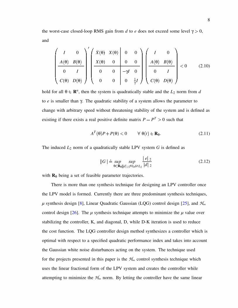
8
the worst-case closed-loop RMS gain from d to e does not exceed some level γ ( 0,
and !I 0
Aθ B
θ
0 I
Cθ D
θ
"$#######%* !
Xθ X
θ 0 0
Xθ 0 0 0
0 0 + γI 0
0 0 0 1γ I
"$#######% !
I 0
Aθ B
θ
0 I
Cθ D
θ
"$#######% , 0 (2.10)
hold for all θ - Rn, then the system is quadratically stable and the L2 norm from d
to e is smaller than γ. The quadratic stability of a system allows the parameter to
change with arbitrary speed without threatening stability of the system and is defined as
existing if there exists a real positive definite matrix P PT ( 0 such that
AT θ P Pθ , 0 . θ
t )- Rθ
(2.11)
The induced L2 norm of a quadratically stable LPV system G is defined as/G/ sup
θ 0 Rθ
sup1d1
2 2 0 3 d 0 L2
/e/
2/d/
2(2.12)
with Rθ being a set of feasible parameter trajectories.
There is more than one synthesis technique for designing an LPV controller once
the LPV model is formed. Currently there are three predominant synthesis techniques,
µ synthesis design [8], Linear Quadratic Gaussian (LQG) control design [25], and H∞
control design [26]. The µ synthesis technique attempts to minimize the µ value over
stabilizing the controller, K, and diagonal, D, while D-K iteration is used to reduce
the cost function. The LQG controller design method synthesizes a controller which is
optimal with respect to a specified quadratic performance index and takes into account
the Gaussian white noise disturbances acting on the system. The technique used
for the projects presented in this paper is the H∞ control synthesis technique which
uses the linear fractional form of the LPV system and creates the controller while
attempting to minimize the H∞ norm. By letting the controller have the same linear
9
fractional relationship with the varying parameters as the LPV system the H∞ control
problem is formulated using linear matrix inequalities (LMI). The appearance of LMIs
in the control synthesis shows how the control problem is a convex optimization
problem [27], as was described in the previous example. Another example of creating
a convex optimization problem with LMI expressions for the use of finding an LPV
controller for the attitude control of an X-33 is presented in [28].
The main benefit of using the LPV framework is that it allows gain-scheduled
controllers to be treated as a single entity, with the gain-scheduling being achieved with
the parameter-dependent controller and automatic interpolation law, which removes the
ad-hoc scheduling schemes that were necessary in the past.

CHAPTER 3LINEAR PARAMETER-VARYING CONTROL FOR AN F/A-18
3.1 Problem Statement
Several control designs have been applied to the control of F-18 aircraft. A
controller was designed using H∞ and µ synthesis techniques for a single flight
condition [29]. Though this technique works well for a single point in the flight
envelope a type of gain-scheduling is necessary for controlling the F/A-18 throughout
its operating domain. A longitudinal variable structure controller was created for an
F-18 model with parameter perturbations [30]. Though this technique can attain the
conventional goals of stability and tracking for uncertain nonlinear plants, a reference
trajectory for tracking control must be specified, which indicates that the controller
cannot operate over a large flight envelope. A lateral-directional controller was created
using µ synthesis with parametric uncertainty to account for gain differences between a
nominal model and trim models and multiplicative uncertainty to account for changes
between a nominal model and other trim models within the chosen flight envelope [31].
Because this technique uses constant blocks of uncertainty instead of gain-scheduling
the flight envelope used for the project had to be small, M 54 0 35055 6 and altitude74 20
28 6 k f t. Gain-scheduled approximations to H∞ controllers for the F/A-18
Active Aeroelastic Wing, located at NASA Langley Research Center, were developed
within another project [32]. Point design controllers were created within a small flight
envelope and then a scheduling scheme of the gains had to be formed. A multivariable
LPV controller was designed using H∞ synthesis for the F/A-18 System Research
Aircraft (SRA), located at NASA Langley Research Center, in [33]. Though this
technique is also chosen for control synthesis in the project presented in this chapter,
the flight envelope that the controller had to operate within is smaller in [33], with
10

11
M 74 0 35070 6 and altitude 84 15
32 6 k f t. A similar project involving an LPV
controller for the F/A-18 SRA, in [18], uses the same synthesis technique but uses an
even smaller flight envelope, M 94 0 45055 6 and altitude :4 20
25 6 k f t, than [33].
The project presented in this study discusses the formation and simulations of a
linear parameter-varying controller for the longitudinal dynamics of an F/A-18 over a
chosen flight envelope. The F/A-18, shown in Figure 3–1, has a ceiling of 50,000+ f t
and a speed of M=1.7+. As the aircraft’s altitude varies so does the air density which
affects the aircraft’s response to control surface deflections. Furthermore, the amount of
deflection necessary for a particular maneuver varies as the Mach number varies. These
aerodynamic changes that occur with the large range in altitude and Mach number
make it necessary to incorporate a gain scheduling technique for control. The flight
envelope for this project is limited to Mach numbers from 0.4 to 0.8, which includes
both incompressible and compressible subsonic flows, and an altitude range from
10,000 f t to 30,000 f t, which includes a density change of roughly 0.9 E ; 3 slug < f t3.
Figure 3–1: F/A-18
The flight envelope can also be considered the parameter space for which the
LPV controller will be designed. The parameter space is two dimensional with the first
parameter dimension being Mach number and the second parameter dimension being
altitude. Originally four points within this two-dimensional parameter space were to be
used to design the LPV controller and are listed in Table 3–1. However, the dynamic

12
pressure, q, for the model at Mach=0.40 at an altitude of 30 kft, P4, was too low to
control and therefore the model was discarded.
Table 3–1: Original Design Points
Design Point Mach Number Altitude ( f t)P1 0.4 10,000P2 0.8 10,000P3 0.8 30,000P4 0.4 30,000
The controller performance is tested with each of the remaining models and with
a model whose dynamics represent the aircraft at a Mach number of 0.6 and at an
altitude of 20,000 ft. A depiction of the flight envelope which represents the parameter
space and the placement of the models used for this project are shown in Figure 3–2.
0.3 0.4 0.5 0.6 0.7 0.8 0.95
10
15
20
25
30
35
P1
P2
P3
PA
Mach Number
Alti
tude
(kft
)
Design PointDesign PointDesign PointAnalysis Point
Figure 3–2: Flight Envelope/Parameter Space
3.2 Open-loop Dynamics
The F/A-18 models used for this project are longitudinal short-period approxima-
tions that were developed with two states, one input and one output. The states include
angle of attack (deg) and pitch rate (deg < sec). The input is the elevator deflection and
the output is pitch rate.

13
The model for the F/A-18 at Mach=0.40 at an altitude of 10 kft is given as P1
such that q P1 δ.
P1 + 07433 425
6200 + 0
5642+ 0
0022 + 0
4064 + 0
0662
0 573 0
(3.1)
The model for the F-18 at Mach=0.80 at an altitude of 10 kft is given as P2 such
that q P2 δ.
P2 + 18415 853
1909 + 2
0292+ 0
0192 + 0
9431 + 0
2568
0 573 0
(3.2)
The model for the F-18 for Mach=0.80 at an altitude of 30 kft is given as P3 such
that q P3 δ.
P3 + 08399 791
1313 + 0
9314+ 0
0075 + 0
4499 + 0
1190
0 573 0
(3.3)
The model of the analysis point with an altitude of 20,000 ft and Mach=0.6 is
given as PA such that q PA δ.
PA + 08280 617
0114 + 0
8269+ 0
0075 + 0
4499 + 0
0994
0 573 0
(3.4)
The frequency and damping ratio for the each of the models were determined and
are shown in Table 3–2. All of the damping ratios are greater than zero, which affirms
that the models are stable.

14
Table 3–2: Frequency and Damping Ratio of Design and Analysis Models
Model ω ζP1 1.113 0.5166P2 4.257 0.3271P3 2.512 0.2567PA 2.288 0.2764
The linear parameter-varying model for the parameter space is given as Pθ and
is given as q Pθ δ.
P = θ >@?BA P1 CED FGGGGHJI 1 K 0982 427 K 57 I 1 K 465I 0 K 017 I 0 K 5367 I 0 K 1906
0 0 0
LNMMMMO θ1 = t > D FGGGGH 1 K 0016 I 62 K 06 1 K 0978
0 K 0117 0 K 4932 0 K 1378
0 0 0
LNMMMMO θ2 = t >(3.5)
Where θ θ1 0
0 θ2
and where θ1 -P4 0 1 6 represents the systems dependence
on Mach number and θ2 -P4 0 1 6 represents the systems dependence on altitude.
The aircraft flying at a Mach number of 0.4 corresponds to a θ1 0 and at a Mach
number of 0.8 corresponds to a θ1 1. The aircraft flying at an altitude of 10,000 f t
corresponds to a θ2 0 and at an altitude of 30,000 f t corresponds to a θ2 1.
3.3 Control Objectives
The control objective for the F/A-18 longitudinal flight controller is to track a
given pitch rate command to within certain tolerances of a target response generated by
a target model that has desirable dynamics. The commanded pitch rate is a step input
which begins at zero magnitude and becomes 10deg < sec at the time of one second and
remains that magnitude until the simulation ends at ten seconds. The response of the
system with the linear parameter-varying controller to the commanded pitch rate must
have a rise time within Q 0.05 sec of the target rise time, an overshoot within Q 4%
of the target overshoot, and a settling time within Q 0.6 sec of the target settling time.
The controller should also have a level of robustness to account for errors in the signal.
15
3.4 Synthesis
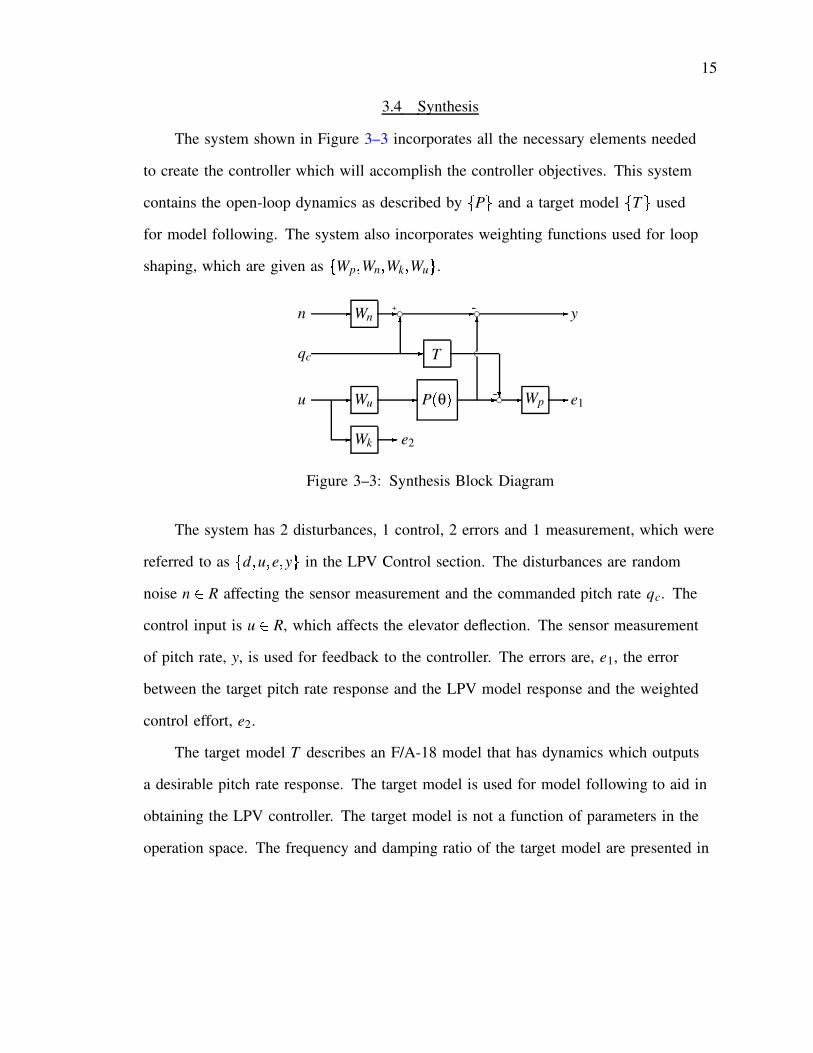
The system shown in Figure 3–3 incorporates all the necessary elements needed
to create the controller which will accomplish the controller objectives. This system
contains the open-loop dynamics as described by P and a target model T used
for model following. The system also incorporates weighting functions used for loop
shaping, which are given as WpWnWkWu .
u & Wu& Wk& e2
& Pθ &- & Wp
& e1
qc&R
ST
Rn & Wn&+ & - & y
Figure 3–3: Synthesis Block Diagram
The system has 2 disturbances, 1 control, 2 errors and 1 measurement, which were
referred to as d u e y in the LPV Control section. The disturbances are random
noise n - R affecting the sensor measurement and the commanded pitch rate qc. The
control input is u - R, which affects the elevator deflection. The sensor measurement
of pitch rate, y, is used for feedback to the controller. The errors are, e1, the error
between the target pitch rate response and the LPV model response and the weighted
control effort, e2.
The target model T describes an F/A-18 model that has dynamics which outputs
a desirable pitch rate response. The target model is used for model following to aid in
obtaining the LPV controller. The target model is not a function of parameters in the
operation space. The frequency and damping ratio of the target model are presented in
16
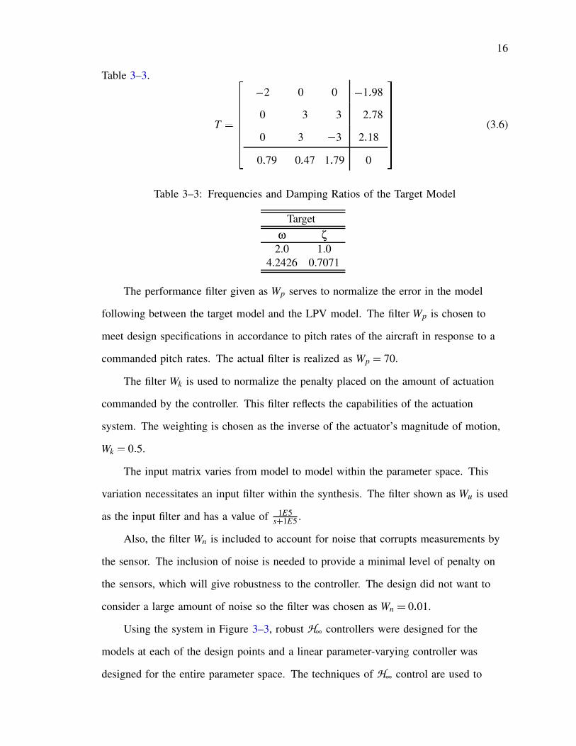
Table 3–3.
T
+ 2 0 0 + 198
0 + 3 + 3 + 278
0 3 + 3 218+ 0
79 + 0
47 1
79 0
(3.6)
Table 3–3: Frequencies and Damping Ratios of the Target Model
Targetω ζ
2.0 1.04.2426 0.7071
The performance filter given as Wp serves to normalize the error in the model
following between the target model and the LPV model. The filter Wp is chosen to
meet design specifications in accordance to pitch rates of the aircraft in response to a
commanded pitch rates. The actual filter is realized as Wp 70.
The filter Wk is used to normalize the penalty placed on the amount of actuation
commanded by the controller. This filter reflects the capabilities of the actuation
system. The weighting is chosen as the inverse of the actuator’s magnitude of motion,
Wk 05.
The input matrix varies from model to model within the parameter space. This
variation necessitates an input filter within the synthesis. The filter shown as Wu is used
as the input filter and has a value of 1E5s T 1E5 .
Also, the filter Wn is included to account for noise that corrupts measurements by
the sensor. The inclusion of noise is needed to provide a minimal level of penalty on
the sensors, which will give robustness to the controller. The design did not want to
consider a large amount of noise so the filter was chosen as Wn 001.
Using the system in Figure 3–3, robust H∞ controllers were designed for the
models at each of the design points and a linear parameter-varying controller was
designed for the entire parameter space. The techniques of H∞ control are used to

17
reduce the induced norm from the input to the weighted errors. The software from the
µ Analysis and Synthesis Toolbox for Matlab is used for the actual computation
of the controller [34]. The same weightings are used to create the controllers in order
to achieve the same performance level for all of the points in the parameter space. The
resulting induced norms achieved by the individual controllers and the LPV controller
are shown in Table 3–4.
Table 3–4: Induced Norms of Closed-Loop System
Open-Loop Model H∞-normP1 0.891P2 0.775P3 0.775
P1 + P3 0.971
It is important to note that all of the closed-loop norms are less than unity. These
magnitudes indicate that the controllers are able to achieve the desired performance and
robustness objectives. The last entry in Table 3–4 is the norm associated with the LPV
controller. Allowing the altitude and Mach number to vary with time increases the
norm as expected. However, this norm did not raise much above the norm associated
with any of the point designed H∞ controllers and stayed below unity. This condition
indicates that the LPV controller is capable of accounting for the time-varying nature
of Mach number and altitude without excessive loss of performance.
3.5 Simulation
The closed-loop dynamics are simulated with a 10deg < s pitch rate step input to
demonstrate the performance of the controller for each of the design models and for the
analysis model. The diagram of the closed-loop system for the models can be seen in
Figure 3–4. The simulations use the same open-loop dynamics but include the linear
parameter-varying controller that was synthesized over the parameter space.
The response to the step input of the LPV controller with the point design models
and the response of the target model are shown in Figure 3–5. The point design

18
δ
&Kθ Pθ & qS
qc'-'
Figure 3–4: Closed-loop Block Diagram
responses only vary roughly 0.2% from the target model response. This characteristic
is due to the LPV controller being created with the models at those points. The
performance of the controller must also be tested with a model that lies away from the
vertices points of the parameter space that were used to create the controller.
0 2 4 6 8 100
2
4
6
8
10
12
Time (s)
Pitc
h R
ate
(deg
/sec
)
CommandTargetP
1P
2P
3
Figure 3–5: Pitch Rate for Design Points
The analysis point was chosen to be the farthest from the vertices of the parameter
space which results in a Mach number of 0.6 and an altitude of 20,000 f t. The
responses of the analysis model and the target model, using the same step command
that was used for the point design simulation, are shown in Figure 3–6. The results
appear to be quite close to the target response. Numerical results were pulled from the
plot to make a closer comparison and are shown in Table 3–5.
The same time response and delay time are apparent for both the analysis model
and target model responses. The settling time of the analysis model response lags the
target response by 0.5 seconds, which is within the control objectives. The maximum

19
0 2 4 6 8 100
2
4
6
8
10
12
Time (s)
Pitc
h R
ate
(deg
/sec
)
CommandTargetP
A
Figure 3–6: Pitch Rate for Analysis Point
Table 3–5: Numerical Results
Target Model Analysis ModelRise Time 0.21 sec 0.21 sec
Settling Time 1.63 sec 2.13 secPeak Overshoot 5 % 1.2 %
overshoot of the analysis model response was less than that of the target model
response and remains within the bounds of the controller objective.
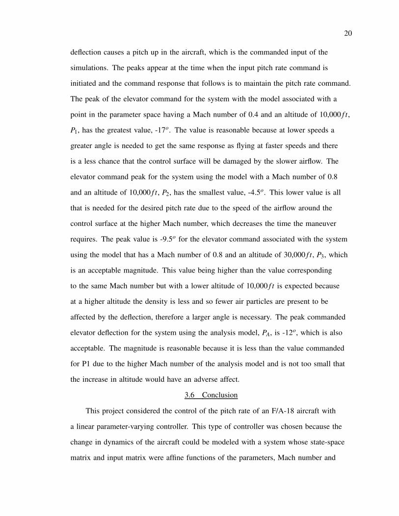
The controller commanded elevator deflection from the simulations is shown in
Figure 3–7 and is used to determine if the actuation of the elevator is reasonable for
each of the tested models. All of the values are negative because a negative elevator
0 2 4 6 8 10−20
−15
−10
−5
0
Time (s)
Com
man
ded
Ele
vato
r Def
lect
ion
(deg
)
PA
P1
P2
P3
Figure 3–7: Controller Elevator Deflection
20
deflection causes a pitch up in the aircraft, which is the commanded input of the
simulations. The peaks appear at the time when the input pitch rate command is
initiated and the command response that follows is to maintain the pitch rate command.
The peak of the elevator command for the system with the model associated with a
point in the parameter space having a Mach number of 0.4 and an altitude of 10,000 f t,
P1, has the greatest value, -17o. The value is reasonable because at lower speeds a
greater angle is needed to get the same response as flying at faster speeds and there
is a less chance that the control surface will be damaged by the slower airflow. The
elevator command peak for the system using the model with a Mach number of 0.8
and an altitude of 10,000 f t, P2, has the smallest value, -4.5o. This lower value is all
that is needed for the desired pitch rate due to the speed of the airflow around the
control surface at the higher Mach number, which decreases the time the maneuver
requires. The peak value is -9.5o for the elevator command associated with the system
using the model that has a Mach number of 0.8 and an altitude of 30,000 f t, P3, which
is an acceptable magnitude. This value being higher than the value corresponding
to the same Mach number but with a lower altitude of 10,000 f t is expected because
at a higher altitude the density is less and so fewer air particles are present to be
affected by the deflection, therefore a larger angle is necessary. The peak commanded
elevator deflection for the system using the analysis model, PA, is -12o, which is also
acceptable. The magnitude is reasonable because it is less than the value commanded
for P1 due to the higher Mach number of the analysis model and is not too small that
the increase in altitude would have an adverse affect.
3.6 Conclusion
This project considered the control of the pitch rate of an F/A-18 aircraft with
a linear parameter-varying controller. This type of controller was chosen because the
change in dynamics of the aircraft could be modeled with a system whose state-space
matrix and input matrix were affine functions of the parameters, Mach number and

21
altitude. Once the controller was created, it was tested at certain points within the
parameter space using a step pitch rate input. The results allow for the conclusion
that the LPV controller performed the specified objectives and is therefore a sufficient
controller for the F/A-18 model presented in this project.

CHAPTER 4LINEAR PARAMETER-VARYING CONTROL FOR A HYPERSONIC AIRCRAFT
4.1 Problem Statement
All aircraft flown today fly within the subsonic, transonic and supersonic flight
regimes. The push toward faster and higher flying aircraft has moved the envelope
into the hypersonic regime. This push comes from both military and commercial
groups. The military wants a bomber that can fly at high altitude, over a long range
and at high speeds, so that the vehicle is nearly impossible to shoot down. Commercial
groups would like to have a more reliable way of sending satellites into low earth orbit.
The major problem with the use of rockets is that if something goes wrong during
ascension into orbit the cargo will most likely be destroyed along with the rocket. The
use of a hypersonic aircraft presents a more reliable transportation for the satellite
because if an error did occur during the flight there would be a chance that the aircraft
could maneuver to a landing area.
Though the concept of hypersonic flight has been discussed since the 1950s
the mass construction of hypersonic aircraft has been hindered by the necessity of
the technology and the price of materials that are able to withstand the elements
in which the vehicles must operate. This obstacle may have slowed the creation of
such vehicles but several control theories have still been created. The more popular
control theories include H∞ [35], µ synthesis [36] and linear parameter-varying
control [37]. The theories involving H∞ and µ synthesis, however, only considered
a single flight condition for the hypersonic vehicle. Also, the previous project that
used a linear-parameter varying controller for the hypersonic vehicle ignored the
mode shape of the vehicle and separated the rigid-body dynamics and the structural
dynamics of the hypersonic model. A scheduled longitudinal control scheme was
22

23
created which incorporated a set of parameter controllers, where the parameters were
Mach number and dynamic pressure, and was determined from linear designs using
analytic functions of the parameters [38]. That project focused on the control of
the rigid body dynamics and did not recognize the effect of structural modes on the
response of the hypersonic vehicle. Robust flight control systems are synthesized
for the longitudinal motion of a hypersonic vehicle using stochastic cost functions
and ten design parameters [39]. That project also focused on the control of the rigid
body dynamics of the hypersonic vehicle without addressing structural dynamics.
The control of the longitudinal motion of a hypersonic vehicle was also addressed,
where robust flight control systems with a nonlinear dynamic inversion structure were
synthesized [40]. Nonlinear control laws were designed so the control systems would
operate over a chosen flight envelope. Again, the rigid body dynamics were the focus
of control. A dual neural network structure was developed that served as feedback
control and optimized the vehicles trajectory to pre-specified burnout conditions in
velocity, flight path angle and altitude [41]. That project serves more as an aid in
the study of trajectory optimization than as a control theory for hypersonic vehicles.
Another project applied a hierarchical integrated control methodology to a hypersonic
vehicle to reduce stabilizing control power required for specific flight conditions [42].
That methodology decomposes the hypersonic model into decoupled subsystems,
creates a controller for each subsystem and a control law for each subsystem controller
is derived. The decoupling of a hypersonic system may not be feasible due to the
large degree of coupling between the physical structure and propulsion system of
the vehicle. Also, the creation of separate control laws is laborious compared to
the LPV method which forms an automatic interpolation law. The control of the
lateral dynamic stability characteristics of a hypersonic vehicle for a specified Mach
number and altitude trajectory has also been detailed in a project [43]. The controller
was designed using Multi-Model Eigenstructure, which designs a robust fixed-gain

24
controller that guarantees robust stability and desired flight qualities along a specified
reference trajectory. The controller would need to be altered if the vehicle deviated
from the preset trajectory or if a flight envelope was to be considered. The same
model of the longitudinal dynamics of a typical hypersonic vehicle were used, where
a unified approach to H2 and H∞ optimal control was used to design a controller for
a specific flight condition [44]. A unified approach alleviates difficulties with the
“over crowding” of a system’s roots inside the unit circle along with other numerical
difficulties. Using the technique in that project would require more controllers to be
created at other operating conditions along with a gain-scheduling law if the vehicle’s
operating range spanned more than a single condition.
Some of the challenges of hypersonic flight include the varying of the hypersonic
vehicle’s dynamic characteristics due to a wide range of operating conditions and
mass distributions for which a type of gain-scheduling technique appears to be
essential [45, 46]. Further discussion of a typical hypersonic vehicle’s dynamics
addresses how the combination of the propulsion system and aeroelastic effects
contribute to the overall dynamic character of the vehicle, which presents the need
of structural dynamic controller [47]. This necessity is the motivation for the project
presented in this chapter.
The controller designed for the hypersonic vehicle for this project was split into
an inner-loop controller and an outer-loop controller. The inner-loop controller is an
LPV controller which must actively damp the structural modes across a temperature
range. Unlike previous hypersonic controls, this controller will focus on the damping
of the mode shape that is associated with the structural dynamics of the vehicle, which
will operate throughout a range of a specific operating parameter and for which the
hypersonic model’s rigid-body and structural dynamics will not be separated. The
outer-loop controller of the aircraft will be a rigid-body controller which will work as
25
a traditional flight controller for rigid aircraft and will be designed in a future project.
The inner-loop structural damping controller is the focus of this project.
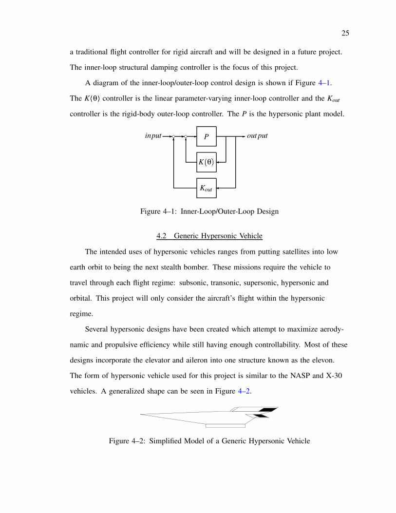
A diagram of the inner-loop/outer-loop control design is shown if Figure 4–1.
The Kθ controller is the linear parameter-varying inner-loop controller and the Kout
controller is the rigid-body outer-loop controller. The P is the hypersonic plant model.
Kout
Kθ P&&&input & out putR R ''
Figure 4–1: Inner-Loop/Outer-Loop Design
4.2 Generic Hypersonic Vehicle
The intended uses of hypersonic vehicles ranges from putting satellites into low
earth orbit to being the next stealth bomber. These missions require the vehicle to
travel through each flight regime: subsonic, transonic, supersonic, hypersonic and
orbital. This project will only consider the aircraft’s flight within the hypersonic
regime.
Several hypersonic designs have been created which attempt to maximize aerody-
namic and propulsive efficiency while still having enough controllability. Most of these
designs incorporate the elevator and aileron into one structure known as the elevon.
The form of hypersonic vehicle used for this project is similar to the NASP and X-30
vehicles. A generalized shape can be seen in Figure 4–2.
Figure 4–2: Simplified Model of a Generic Hypersonic Vehicle

26
This configuration of a hypersonic vehicle combines the fuselage with the
propulsion system. This combination greatly affects the flight dynamics of the vehicle.
The forebody of the vehicle acts as the compressor for the engine. The air flow
through this compressor creates a pitch up moment. The aftbody of the vehicle acts
as the exit nozzle for the engine. The airflow through the exit nozzle creates a pitch
down moment. Also, a change in angle of attack or sideslip affects the engine inlet
conditions which changes the propulsion performance. To create a controller for
this type of vehicle the angle of attack, pitch angle and pitch rate are measured for
feedback to the controller.
Another area of hypersonic flight that must be considered when creating a
controller is the speed, and consequently temperature, at which the vehicle flies. As the
vehicle enters the hypersonic regime, the strength of shock waves increase and lead to
higher temperatures in the region between the shock and the body. As Mach number
increases further, the shock layer temperature becomes large enough that chemical
reactions occur in the air. Also, an increase in temperature effects the structural
dynamics of the vehicle in that there is a reduction in the frequency of the structural
modes. Therefore, the controller created in this project will consider temperature as the
flight parameter.
4.3 Hypersonic Model
The hypersonic model [48] used for this project was limited to the longitudinal
motion and was developed with seven states, three inputs and six outputs. The states
include altitude, velocity, angle of attack, pitch angle, pitch rate, and two elastic states
for the fuselage bending mode. The inputs include elevon deflection, diffuser area
ratio and fuel flow ratio. The outputs include angle of attack, pitch rate at forebody,
pitch rate at aftbody, combustor inlet pressure, Mach and thrust which will be used
as feedback to the controller. Only the angle of attack and the two pitch rates are to
be used as feedback to the controller due to their strong dependence on the structural

27
dynamics. Aerodynamic, inertial, propulsive, and elastic forces were used to derive the
equations of motion for the hypersonic vehicle [37]. The model dimensions and flight
conditions are shown in Table 4–1.
Table 4–1: Model Dimensions and Flight Conditions
Length 150 f tMass 300,000 lb
Height 100,000 f tMach 8
Dynamic Pressure 1017 ps f
4.4 Linear Parameter-Varying System
The time-varying operating parameters, θ, are flight parameters which affect the
aircraft during flight. These parameters are measured by sensors on the aircraft and
are sent to the controller. This project takes into account only one flight parameter,
temperature, due to the large affect that temperature has on a hypersonic vehicle’s
structural dynamics. This parameter will have a range from (0oF to 5000oF) to match
the temperature ranges noted for the hypersonic flight of the X-30 and the HyperX
vehicles [49]. The parameter dependence of the model is shown in the matrices below,
θ 0 for the coldest temperature and θ 1 for the hottest temperature within the
range. As the flight parameter, temperature, changes during flight so does the amount
it affects changes in the aircraft. This problem can be compensated with the use of
weighting functions which will be discussed in the next section.
Aθ VU A W θ U Aθ W (4.1)

28
A XYZZZZZZZZZZZZZZZZ[
0 0 ; 7 \ 9248E3 7 \ 9248E3 0 0 0
1 \ 5026E ; 4 ; 3 \ 2374E ; 3 ; 5 \ 2818E1 ; 3 \ 2200E1 2 \ 3762E ; 2 5 \ 7314E ; 1 7 \ 5583E ; 3
1 \ 1744E ; 7 ; 3 \ 1848E ; 7 ; 3 \ 3921E ; 2 0 1 1 \ 4681E ; 4 2 \ 8801E ; 6
0 0 0 0 1 0 0; 5 \ 7586E ; 6 9 \ 6079E ; 6 1 \ 5833E0 0 ; 5 \ 1609E ; 2 9 \ 2411E ; 2 ; 1 \ 8285E ; 4
0 0 0 0 0 0 1; 7 \ 4858E ; 1 1 \ 0158E ; 1 2 \ 4280E3 0 ; 7 \ 4847E0 ; 3 \ 1086E2 ; 9 \ 4975E ; 1
] ^^^^^^^^^^^^^^^^_ (4.2)
Aθ
0 0 0 0 0 0 0
0 0 0 0 0 0 0
0 0 0 0 0 0 0
0 0 0 0 0 0 0
0 0 0 0 0 0 0
0 0 0 0 0 0 0
0 0 0 0 0 + 25E2 + 0
2
(4.3)
B
0 0 0+ 6435E1 + 7
462E1 1
261E3+ 1
448E + 2 + 1
596E + 2 + 2
253E + 2
0 0 0+ 2455E0 8
111E + 1 5
190E0
0 0 0
6740E2 + 2
925E1 2
209E2
(4.4)
Cθ `U C W θ U Cθ W (4.5)

29
C abccccccccccccccd
0 0 1 0 0 1 e 7453E f 2 0
0 0 0 0 1 0 1 e 7453E f 2
0 0 0 0 1 0 f 1 e 7453E f 2f 4 e 6971E f 5 2 e 0641E f 4 6 e 2428E0 0 f 1 e 0921E f 2 1 e 0896E f 1 0f 5 e 3709E f 6 1 e 0095E f 3 0 0 0 0 0f 3 e 5754E f 1 6 e 0213E f 1 1 e 8399E4 0 f 3 e 2185E1 3 e 2112E2 0
gihhhhhhhhhhhhhhj(4.6)
Cθ
0 0 0 0 0 C16 lk 1
05 0
0 0 0 0 0 0 C17 mk 0
05
0 0 0 0 0 0 C227 lk 0
05
0 0 0 0 0 C236 lk 0
05 0
0 0 0 0 0 0 0
0 0 0 0 0 C256 lk 0
05 0
(4.7)
D
0 0 0
0 0 0
0 0 0
0 + 7229 0
0 0 0
0 + 3158E4 5
995E5
(4.8)
As seen in the linear parameter-varying matrices above, both the state matrix 4 A 6and the observation matrix 4C 6 change with temperature. It is common for the state
matrix to change as operating parameters change, but it is not common, in traditional
aircraft, for the observation matrix to change. This change in the observation matrix
accounts for the mode shape changes of the hypersonic vehicle.
The modes of the hypersonic model are shown for different temperatures in
Table 4–2 . The table shows the frequency of each of the modes and the damping

30
corresponding to the frequency. The four modes of the open-loop dynamics are (i)
a height mode, (ii) an unstable phugoid-like mode, (iii) an unstable pitch mode and
(iv) the structural mode. As can be seen in the table, the structural mode for the
model at the cold temperature has a higher frequency than the structural mode at the
hot temperature. Minimizing the affect that the temperature has on this mode is the
objective of the inner-loop LPV controller.
Table 4–2: Modes of the Hypersonic Model
Cold HotMode ω
rad < sec ζ ω
rad < sec ζ
i 0.0024 1.00 0.0024 1.00ii 0.1666 1.00 0.1790 1.00
0.1677 -1.00 0.1804 -1.00iii 1.462 -1.00 1.518 -1.00
1.554 1.00 1.608 1.00iv 17.65 0.0268 15.84 0.0062
4.5 Control Design
The control objective of the linear parameter-varying controller is to damp out
the structural mode in order to minimize the affect that temperature has on the model.
The controller should also contain a level of robustness to account for errors in signals.
A system was created that incorporated the necessary elements to accomplish these
objectives. The first step in the finding the LPV controller was to create a synthesis
model shown in Figure 4–3.
The system has 2 disturbance inputs, 1 control input, 2 error outputs and 1
measurement output. The disturbance vector n - R3 is random noise which affects
sensor measurements. The incorporation of noise creates a small level of robustness
within the controller. The disturbance δ - R is a commanded elevon deflection. The
control input u - R is the excitation from the controller affecting the control actuators.
The error ep - R is the weighted measurements of the angle of attack by the sensors.
The error ek - R is the error of the control actuation. The measurements in the vector

31
u & Wk& ek
R+δ & & Pθ SSSWn&n &+ S&+ S&+ S
y
& T &-R & Wp& ep
X 'S
Figure 4–3: Synthesis Block Diagram
y - R3 are the sensor measurements of angle of attack, pitch rate at the forebody and
pitch rate at the aftbody which will be used for feedback to the controller.
The open-loop dynamics of the LPV system is described by Pθ . Where,
Pθ A
θ B
Cθ D
(4.9)
A target model, T , is created to describe a hypersonic model with desirable
structural damping and therefore incorporates the controller objective. The target model
was used for model following to aid in obtaining the LPV controller. The target model
modes and corresponding damping are shown in Table 4–3. The target model has
a large magnitude of damping corresponding to its structural mode compared to the
damping found in the hot and cold temperature models. It is this amount of damping
that the controller must impose upon the hypersonic model throughout the temperature
range.
The performance filter, Wp, would normally be used to define the design specifi-
cations in the frequency domain. For this synthesis Wp was made equal to 1.5 which

32
Table 4–3: Modes of the Target Model
TargetMode ω
rad < sec ζ
i 0.0024 1.00ii 0.1728 1.00
0.1735 -1.00iii 1.478 -1.00
1.590 1.00iv 16.75 0 .2381
allows measurements through all frequencies to pass through with only a slight de-
crease in gain. This passage throughout all frequencies was allowed because of the
simple controller X which was incorporated into the system to stabilize the vehicle.
A simple H∞ controller, X , is created in order to stabilize the rigid-body dynamics
of the hypersonic vehicle without an affect on the structural mode. This small con-
troller was implemented so that the structural dynamics controller would not try to alter
the rigid-body dynamics. Stabilizing the rigid-body of the model allows the creation of
the LPV controller for the structural dynamics.
The filter, Wn, passes an allowed amount of noise to the sensors. Wn 001
because only a small amount of noise was needed to pass into the system to ensure that
the controller would be robust. The filter, Wk, is used to normalize the restriction on
the amount of actuation the controller commands. Wk was chosen so that the weighting
is the inverse of the actuators’ magnitudes of motion, Wk s T 180s T 1000 .
The results of the open-loop synthesis were then used to create the LPV controller,
Kθ , using the LMI ControlToolbox [50]. To determine how well the controller would
work the H∞ norm was found for the system throughout the temperature range, along
with the H∞ norm for the system at the cold temperature and at the hot temperature.
The frequencies at which the H∞ norm occurred for the model at the hot and cold
temperatures were also found. The results of this test are shown in Table 4–4. The
magnitude of the H∞ norms of the model at the hot and cold temperatures mainly

33
draws from the connection of the first input, q, to the first output, the ep, meaning that
the largest error comes from the performance of the angle of attack meeting the elevon
deflection command.
Table 4–4: Open-Loop Synthesis Norms
H∞ norm ωrad < sec
System 0.9386Cold 0.9159 17.90Hot 0.91196 19.81
H∞ controllers were made specifically for the model at the cold temperature and
the model at the hot temperature. The H∞ norms of these point designs were found
and used to compare to those found for the full LPV system. The results are shown in
Table 4–5.
Table 4–5: Point Design Norms
H∞ normCold 0.1476Hot 0.1679
Compared to the norms of the system with the LPV controller at the hot and cold
temperatures and the norms of H∞ controllers at the point designs, the norm of the
LPV system is relatively high. This difference results from the time-varying nature
of the parameters of the system. Despite this increase in magnitude the LPV system’s
H∞ norm is still less than one, showing that the LPV controller that was created is
capable of controlling the system.
4.6 Simulation
4.6.1 Open-Loop Simulation
The frequency response of the open-loop transfer function between the elevon
defection and the angle of attack for the target model, cold model and hot model is
shown in Figure 4–4. The plot of the response in the frequency domain demonstrates
the need for the control of the structural dynamics. The peak in the response that
34
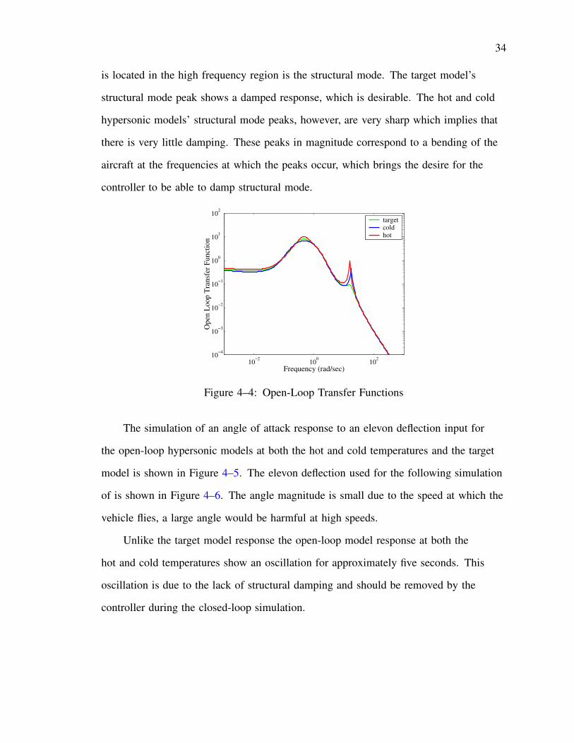
is located in the high frequency region is the structural mode. The target model’s
structural mode peak shows a damped response, which is desirable. The hot and cold
hypersonic models’ structural mode peaks, however, are very sharp which implies that
there is very little damping. These peaks in magnitude correspond to a bending of the
aircraft at the frequencies at which the peaks occur, which brings the desire for the
controller to be able to damp structural mode.
10−2 100 10210−4
10−3
10−2
10−1
100
101
102
Frequency (rad/sec)
Ope
n L
oop
Tra
nsfe
r Fun
ctio
n
targetcoldhot
Figure 4–4: Open-Loop Transfer Functions
The simulation of an angle of attack response to an elevon deflection input for
the open-loop hypersonic models at both the hot and cold temperatures and the target
model is shown in Figure 4–5. The elevon deflection used for the following simulation
of is shown in Figure 4–6. The angle magnitude is small due to the speed at which the
vehicle flies, a large angle would be harmful at high speeds.
Unlike the target model response the open-loop model response at both the
hot and cold temperatures show an oscillation for approximately five seconds. This
oscillation is due to the lack of structural damping and should be removed by the
controller during the closed-loop simulation.

35
0 5 10 15−4
−3
−2
−1
0
1
2
3
Time (s)
Ang
le o
f Atta
ck (d
eg)
targetcoldhot
Figure 4–5: Open-Loop Angle of Attack Result
0 5 10 150
1
2
3
4
5
6
Time(s)
Inpu
t Ele
von
Def
lect
ion
(deg
)
Input Elevon Deflection
Figure 4–6: Input Elevon Deflection
4.6.2 Closed-Loop Simulation
The closed-loop dynamics are simulated to demonstrate the performance of
the controller for the hypersonic models at both the hot and cold temperature. The
closed-loop system for both models can be seen in Figure 4–7.
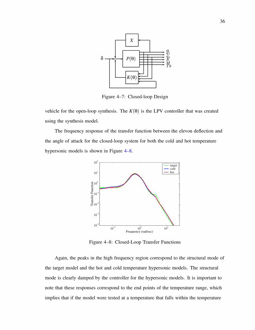
The system shown in Figure 4–7 has one input signal and six output signals. The
input signal δ remains the elevon deflection. The outputs include angle of attack (α),
pitch rate at forebody (q f ), pitch rate at aftbody (qa), combustor inlet pressure (Pi),
Mach (M) and thrust (T h). The X is the same simple controller used to stabilize the
36
Kθ
Rδ & & Pθ &
T h&
M& Pi
& qa& q f& α
'''''XS
Figure 4–7: Closed-loop Design
vehicle for the open-loop synthesis. The Kθ is the LPV controller that was created
using the synthesis model.
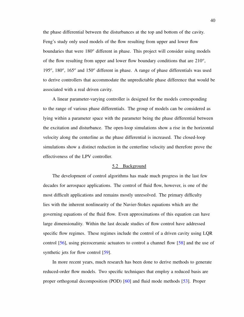
The frequency response of the transfer function between the elevon deflection and
the angle of attack for the closed-loop system for both the cold and hot temperature
hypersonic models is shown in Figure 4–8.
10−2 100 10210−4
10−3
10−2
10−1
100
101
102
Frequency (rad/sec)
Tra
nsfe
r Fun
ctio
n
targetcoldhot
Figure 4–8: Closed-Loop Transfer Functions
Again, the peaks in the high frequency region correspond to the structural mode of
the target model and the hot and cold temperature hypersonic models. The structural
mode is clearly damped by the controller for the hypersonic models. It is important to
note that these responses correspond to the end points of the temperature range, which
implies that if the model were tested at a temperature that falls within the temperature

37
range that a similar damped peak would result. So the control objective of damping the
structural mode was fulfilled by the LPV controller.
The closed-loop simulation of the angle of attack response to the same elevon
deflection used in the open-loop simulation is shown in Figure 4–9. The results are
again presented for the system at both the hot and cold temperatures and for the target
model.
0 5 10 15−4
−3
−2
−1
0
1
2
3
Time (s)
Ang
le o
f Atta
ck (d
eg)
targetcoldhot
Figure 4–9: Closed-Loop Angle of Attack Result
As can be seen, the oscillations that were apparent in the open-loop simulation
have been removed by the controller. This response is due to the damping which the
controller imposed on the system. The hypersonic models’ responses also follow the
target model response more closely throughout the simulation.
The controller commanded elevon deflection in Figure 4–10 is plotted for the
closed-loop simulation in order to verify that the motion commanded did not violate
the limited motion due to the high Mach number. Because the command never exceeds
a magnitude of 5o the command does not violate the constraint associated with the
elevon actuator. The corresponding deflection rate in Figure 4–11 is plotted to verify
that the command does not violate the motion tolerances of the elevon actuator. The
magnitude of the deflection rate is within the limits associated with the actuator.

38
0 5 10 15−4
−3
−2
−1
0
1
2
3
4
5
Time(s)
Ele
von
Def
lect
ion
(deg
)
cold commandhot command
Figure 4–10: Elevon Deflection Command
0 5 10 15
−60
−40
−20
0
20
40
60
80
Time(s)
Ele
von
Def
lect
ion
Rat
e (d
eg/s
)
coldhot
Figure 4–11: Elevon Deflection Rate
4.7 Conclusion
This project considered the control of the structural dynamics of a hypersonic
vehicle with a linear parameter-varying controller. This type of controller was chosen
because the change in the dynamics of the hypersonic vehicle could be modeled
with a system whose state-space matrix and observation matrix were affine functions
of the parameter, temperature. Once this controller was created, it was tested over
a temperature range with an elevon deflection input. The results allowed for the
conclusion that the LPV controller performed the specified objective and is therefore a
sufficient controller for the hypersonic model presented in this project.

CHAPTER 5LINEAR PARAMETER-VARYING CONTROL FOR A DRIVEN CAVITY
5.1 Problem Statement
Research into flow control techniques has been continually evolving as related
technologies mature. These technologies include hardware development, such as
sensors and actuators [51], and software development, such as models and simula-
tions [52], associated with fluid dynamics. In each case, the technologies are being
developed with careful consideration of the requirements for control design and
implementation [53].
A particular challenge for flow control has been the development of open-loop
models for which controllers can be designed. The equations of motion for such
dynamics are well known and detailed computational simulations are routinely
performed. Unfortunately, the equations of motion are highly nonlinear and no methods
are currently practical that can directly utilize them for feedback control synthesis.
A recent study has shown that models can indeed be generated that are amenable
to control a specific type of flow [54]. The system in that study is restricted to creep-
ing flow in a driven cavity. Specifically, the left and right sides of the cavity have zero
flow velocity whereas the top and bottom boundaries are driven by exogenous flow
with fixed velocity and frequency. Models are generated by considering the linearized
dynamics associated with modes obtained via proper orthogonal decomposition [55].
These modes were used to derive controllers for disturbance rejection. The derived
controllers were able to keep the flow nearly stationary at various points throughout the
cavity for varying flow regime despite the exogenous input[56, 57].
This project extends the work of Feng [54] to consider different flow conditions
for the driven cavity. Specifically, the open-loop models are generated by considering
39
40
the phase differential between the disturbances at the top and bottom of the cavity.
Feng’s study only used models of the flow resulting from upper and lower flow
boundaries that were 180o different in phase. This project will consider using models
of the flow resulting from upper and lower flow boundary conditions that are 210o,
195o, 180o, 165o and 150o different in phase. A range of phase differentials was used
to derive controllers that accommodate the unpredictable phase difference that would be
associated with a real driven cavity.
A linear parameter-varying controller is designed for the models corresponding
to the range of various phase differentials. The group of models can be considered as
lying within a parameter space with the parameter being the phase differential between
the excitation and disturbance. The open-loop simulations show a rise in the horizontal
velocity along the centerline as the phase differential is increased. The closed-loop
simulations show a distinct reduction in the centerline velocity and therefore prove the
effectiveness of the LPV controller.
5.2 Background
The development of control algorithms has made much progress in the last few
decades for aerospace applications. The control of fluid flow, however, is one of the
most difficult applications and remains mostly unresolved. The primary difficulty
lies with the inherent nonlinearity of the Navier-Stokes equations which are the
governing equations of the fluid flow. Even approximations of this equation can have
large dimensionality. Within the last decade studies of flow control have addressed
specific flow regimes. These regimes include the control of a driven cavity using LQR
control [56], using piezoceramic actuators to control a channel flow [58] and the use of
synthetic jets for flow control [59].
In more recent years, much research has been done to derive methods to generate
reduced-order flow models. Two specific techniques that employ a reduced basis are
proper orthogonal decomposition (POD) [60] and fluid mode methods [53]. Proper

41
orthogonal decomposition is a model reduction technique in which the most energetic
modes are systematically extracted from numerical simulations. This method of
reduction was used to create the models used in this project. The fluid mode method
uses basis functions which are closely related to the physics of the problem being
solved.
Another area of interest for this project is what is known as Stokes or creeping
flow. The limitations of using Stokes flow are that the flow must be incompressible and
have a Reynolds number less than one. One side effect of lowering a flow’s Reynolds
number is that the acceleration term within the Navier-Stokes governing equation
becomes small compared to the viscous force term. This change allows the equation to
be simplified into the linear Stokes equation [61, 62].
5.3 Driven Cavity Geometry
This project will investigate flow control for the cavity shown in Figure 5–1,
where h0t is the velocity along the top of the cavity, β
t is the velocity along the
bottom of the cavity and Γ ΓL n ΓR n ΓT n ΓB is the boundary of the domain. This
cavity is enclosed by rigid walls with no-slip boundary conditions on the right and left
sides. The top and bottom, however, have nonzero boundary conditions in general.
Figure 5–1: Stokes Driven Cavity Flow Problem
The flow at the top and bottom boundaries have uniform spatial distribution. This
restriction implies that the flow at any point along the upper boundary is identical
42
to the flow at any other point along the upper boundary. Similarly, the flow at any
point along the bottom boundary is identical to the flow at any other point along the
bottom boundary. Such a perfect distribution is not possible because of the singularity
at the points on the corners where the flow is moving on the horizontal boundary but
stationary on the vertical boundary. Such a situation is obviously an approximation, but
this example does serve as an initial problem to demonstrate the methodology.
The approximation within the 2-D cavity is based on a grid with an index of
21x21 points. It is assumed that the measurements of the flow velocity are taken at
19 points along the horizontal centerline of the cavity, with the outer points lying one
grid point away from the closest boundary wall. These measurements only provide the
horizontal velocity of the flow. Also, the sensors generating these measurements are
assumed to exist within the cavity without altering the flow. Again, such a situation is
obviously an approximation, but the example serves to demonstrate the methodology.
5.4 Governing Equations of Motion
Consider first the unsteady Navier-Stokes equations
ρ∂ oV∂t ρ oV p ∇ oV :+ ∇p µ∆ oV (5.1)
subject to boundary conditions described in the past section. The parameter oV is the
velocity field, p is the pressure, ρ is the density and µ is the viscosity of the fluid. The
constants that will be used to nondimensionalize the problem include a characteristic
dimension L, characteristic velocity Vs, and characteristic
43
frequency f . Non-dimensional variables are defined as
x q) x < L (5.2)
y q y < L (5.3)oV q 9oV < Vs (5.4)
p q p < ρLVs (5.5)
t q t f (5.6)
The resulting non-dimensional Navier-Stokes equation can be written as
Re p St∂ oV q∂t q Re r oV q p ∇ qsoV qut :+ Re p St∇ q p q ∆ qvoV q (5.7)
where St is Strouhal number defined as
St L fVs
(5.8)
Define
λ Re p St ρL2 fµ
(5.9)
This project will consider flow such that λ w O1 and the Reynolds number is
Re=0.1. In this case, the terms on the right hand side will balance the first term on the
left hand side and the second term will be neglected.
Define the constant
θ 1λ 1
Re p St(5.10)
Finally, the governing equations for the approximation of Stokes flow is achieved
∂ oV q∂t q + θ∆ oV q ∇p 0 (5.11)
For convenience, Equation 5.11 is rewritten as
∂ oV∂t+ θ∆ oV ∇p 0 (5.12)
44
while keeping in mind that these are nondimensional variables.
5.5 Reduced-Order Linear Dynamics
For the geometry depicted in Figure 5–1, define the flow domain as Ω. The
boundary of the fluid flow domain is given by
∂Ω ΓT n ΓB n ΓL n ΓR (5.13)
It is assumed that the input velocity imparted by the moving wall can be repre-
sented in term of Nc functions ogii 1
nc. Each of the functions ogi are defined on
the entire domain Ω, but are assumed to exhibit specific properties on the boundary. It
is required that ogi x ∂Ωx y 1 f or x - ΓB
0 f or x - ∂Ω z ΓB
(5.14)
Additionally, it is required that ∂Ωogi p ndS 0 (5.15)
for i 1
Nc. This last condition is required to guarantee compatibility of the flow
field with the continuity equation.
The dynamics for incompressible, two-dimensional creeping flows can be repre-
sented in the strong form of Stokes equation by rewriting the Equation 5.12.
∂ oV∂t+ θ∆ oV ∇p of (5.16)
Likewise, the strong form of the continuity equation for incompressible flow is
∇ p oV 0 (5.17)
In these equations, oV is the flow velocity, p is the pressure and of is the body force. It
is assumed that spatially-varying functions oφi , for i 1
Ns have been determined
from the POD procedure which will be discussed in detail later. The functions oφi
constitute the reduced basis used to represent the Ns states in the control model,
45
which include phase differential information. There is a different set of oφi functions
associated with each parameter within the phase differential subspace δ=[150,210],
which is used to create reduced-order models at specific phase differentails. Similarly,
we assume that spatially-varying functions ogi, for i 1
Nc, have likewise been
derived from a simulation or experiment. The functions ogi comprise the influence
functions that determine the controls acting on the fluid flow. It is assumed that these
functions satisfy the following conditions which are conventional in many reduced
basis formulations :
∇ p oφi 0 for i 1
Ns (5.18)
∇ p ogi 0 for i 1
Nc (5.19)oφi x ∂Ω 0 for i 1
Ns (5.20)ogi 0 for x <- ΓB (5.21)
In terms of these reduced basis functions, the velocity appearing in the Stokes equa-
tions is assumed to take the formoV x y t oVMt | NC
∑i 1
ogixy βi
t NS
∑i 1oφixy αi
t (5.22)
To derive a reduced-order model appropriate for control synthesis, it is necessary to
convert the strong form of the governing equations to weak form. The inner product,
bilinear form a p p~ are defined, respectively, as ou ov 4 L2 Ω 6 2 ∆ 2
∑i 1
Ω
uividx (5.23)
a ou ov ∆ θ
2
∑i 1
2
∑j 1
Ω
∂ui
∂xk
∂vi
∂xkdx (5.24)
By substituting the velocity into the strong form of the governing equations, taking
the inner product of the resulting expression with an arbitrary basis function oφi , and
46
integrating over the domain Ω, we obtainNC
∑i 1
ogixy βi
t NS
∑i 1oφixy αi
t oφ j 4 L2 Ω 6 2 a
oVM NC
∑i 1
ogixy βi
t NC
∑i 1oφixy αi
t oφ j r of oφ j t 4 L2 Ω 6 2
(5.25)
The terms are gathered and put the equations in a canonical form appropriate for
control synthesis.
NC
∑i 1
ogi oφ j 4 L2 Ω 6 2βi
t NS
∑i 1
oφi oφ j 4 L2 Ω 6 2αi
t a
oVM oφ j NC
∑i 1
a ogi oφ j βi
t NS
∑i 1
a oφi oφ j αi
t r of oφ j t 4 L2 Ω 6 2
(5.26)
A new set of states that include both the original reduced state variables and the
amplitude of the controls is defined as
Xt α
t
βt B (5.27)
The new set of controls is defined to be the time derivative of the original controls
ut β
t (5.28)
With these definitions of the state Xt and controls u
t , it is possible to write the
weak form of the governing equations asM X
t
A Xt |
B ut
Ct (5.29)
It is important to note that the matrix 4 M 6 will be diagonal if the reduced basis vectors
are derived from a proper orthogonal decomposition. The final form of the reduced

47
state equations can be obtained by premultiplying by the inverse of the matrix 4 M 6Xt
M 1 A Xt
M s 1 QXt
M 1 B ut (5.30)
which can be rewritten in the final form as
Xt 94 A θ 6 X t |P4 B 6 u t |4 E θ t 6 (5.31)
where 4 A θ 6 is a linear function of θ, 4 B 6 is a constant matrix, and 4 E θ t 6 is a
function of h0t .
5.6 Creeping Flow in a Driven Cavity
Since the dynamical model is linear, we can construct oVMt asoVM
t oV0 p h0
t (5.32)
where oV0 is the velocity field of creeping flow when constant horizontal velocity is
imposed on the top of the cavity. It is required that
oV0 x ∂Ωx y 1 f or x - ΓT
0 f or x - ∂Ω z ΓT
(5.33)
Also, we choose Nc 1 and og as the velocity field that corresponds to a constant
horizontal velocity imposed on the bottom wall of the cavity. It is required that
oV0 x ∂Ωx y 1 f or x - ΓB
0 f or x - ∂Ω z ΓB
(5.34)
The velocity can subsequently be decomposed asoV x y t oV0h0t | og x y β t NS
∑i 1oφixy αi
t (5.35)

48
Thus, the reduced-order model in Equation 5.31 can be rewritten explicitly as α
β 4 A1θ 64 A2
θ 6
0 0
α
β 4 E1θ 64 E2 6
0 0
h0
h0 4 B1 61
β (5.36)
Consider just the partition associated with the time-domain equation for α
α A1θ α t | A2
θ β t | B1β
t E1
θ h0
t E2h0
t (5.37)
Formulate the equivalent frequency-domain expression
sαs A1
θ α s A2
θ β s | sB1β
s E1
θ h s | sE2h
s (5.38)

49
A transfer function representation of the inputs to outputs can now be solved.
αs V sE2 E1
θ
s + A1θ h0
s sB1 A2
θ
s + A1θ β
s
A1θ E1
θ | A1
θ E2
I E2
hs
A1 A2 A1B1
I B1
βs
A1θ E1
θ A2
θ
I E2 B1
hs
βs P
s h
s
βs (5.39)
The reduced-order model described by P is a fairly accurate representation of the
open-loop dynamics for Stokes flow in the driven cavity with θ w O1 . All of the
models will be based on a θ 1 in this project. There is a decrease in accuracy as θ
changes from unity because of unmodeled nonlinearities. The linear parameter varying
controller is designed and tested for models over the range of phase differentials
δ 4 150210 6 .
5.7 Excitation Phase Differential
Open-loop models of the flow dynamics are generated by analyzing simulated
responses of the driven cavity. This simulation uses the Stokes flow as the fluid
dynamics. Separate models are generated for each set of flow conditions that corre-
sponded to different relationships between the upper and lower boundaries.
Each of these models have physical limitations associated with them. The
Reynolds number for each model is Re=0.1. The combination of the low Reynolds
number and the approximation of the Navier-Stokes equation creates a flow which is
dominated by viscous effects.

50
The fluid at the upper and lower boundaries was constrained to move at a
sinusoidal frequency with constant amplitude. The frequency of this sinusoidal is
essentially considered a non-dimensional unity because the time scales in the dynamics
are all normalized. This excitation acts as a disturbance that affects the entire flow
within the cavity.
The variations between the flow conditions used for model development were
phase relationships between the upper and lower boundaries. Specifically, the sinu-
soidal flows differed in phase by 210o, 195o, 180o, 165o, and 150o between the upper
and lower boundaries. These phase differences induced different modal structures
within the flow so the various models were generated to represent a basis for this range
of flow conditions.
The reduced-order models associated with each phase differential, which contain
three states, can actually be considered as subspaces of the full-order flow, which
contains 623 states. The exogenous disturbances will, in general, not have a constant
phase differential so the flow field will contain modes associated with many phase dif-
ferentials throughout any time evolution. As such, each reduced-order model represents
a subspace of the modes observed in that full-order flow field. Thus, synthesizing con-
trollers for these models with phase differentials is essentially designing compensators
that are optimal with respect to each subspace.
5.8 Control Design
5.8.1 Control Objectives
The objective of flow control in this project is to reject the effects of the ex-
ogenous disturbance at the top of the driven cavity. Physically, the control seeks to
minimize the horizontal component of the fluid velocity at a set of sensor locations.
These sensors are located at 19 sites evenly distributed along the horizontal centerline
of the cavity. The end sensors are located 1 grid point away from the boundary wall.

51
The controller is designed for disturbance rejection using the model shown in Fig-
ure 5–2. This model contains the open-loop dynamics as described by VmΦΨP .
The weighting functions used for loop shaping are given as WpWnWkWyWhWuWd .
The mathematical objective of the control
design is to choose a K such that the closed-loop transfer function from disturbances to
errors has an induced norm less than unity for all plants within the parameter space.
u
R& Wk
RWa
R∆a
'+ && e2
Wuβ &h & Wh&
Pδ & Ψ
R& Φα &+ & Wp& e1
& Vm S RWy
R+Wn&n & & y
Figure 5–2: Controller Block Diagram
The system has 3 input vectors and 3 output vectors. The inputs are the
random noise n - R 19 affecting the sensor measurements, the exogenous disturbance
h - R affecting the upper boundary of the cavity, and the control input u - R affecting
the lower boundary of the cavity. The outputs are the (frequency domain) weighted
horizontal velocity measurements e1 - R 19, the (frequency domain) weighted control
effort e2 - R , and the sensor measurements y - R 19 used for feedback to the controller.
The open-loop dynamics consist of the cavity’s velocity at the top, a control basis
and flow shape basis. The part of the open-loop dynamics known as Vm is the mean
velocity along the top of the cavity and has the equation Vm hot oVo where ho is the
initial top disturbance and Vo is a static Stokes flow along the top. The control basis
for the plant takes the form Ψβt , which was depicted as og x y β t in the equations
presented in the previous sections, and coincides with the controlled velocity along the

52
bottom of the cavity. The shape of the fluid flow within the cavity is determined by
the flow shape basis Φ. The flow shape can take several forms; for example, the flow
could be one large vortex circling the entire cavity or two vortices of equal size with
opposite rotation that meet along the horizontal center line of the cavity.
The filter given as Wp serves to normalize the measurement of flow velocity
collected by the sensors. This filter achieves loop-shaping that defines the design
specifications in the frequency domain. The filter Wp is chosen to reflect the inverse of
acceptable velocities in response to unity disturbances. The actual filter is realized as
Wp 100 which implies the flow velocities should be less than 0.01 in the closed-loop
system.
The filter Wk is used to normalize the penalty placed on the amount of actuation
commanded by the controller. This filter reflects the capabilities of the actuation
system. The magnitude of motion for the control actuator is allowed to be 02 in the
non-dimensional system. The weighting is chosen as the inverse so that Wk 5.
The creation of a linear parameter-varying controller requires that an output filter
be used because a certain part of the observation matrix and feedthrough matrix vary
with the different plants within the parameter space. The filter Wy is used as the output
filter for this synthesis. The filter was chosen as Wy 1E5s T 1E5 .
Also, the input matrix varies among the different plant models within the param-
eter space. This variation necessitates input filters within the synthesis. The filters
shown as Wu and Wh are used as input filters and have the value of 1E5s T 1E5 .
Multiplicative uncertainty was introduced into the control actuation in order
to increase the system’s robustness with respect to the unmodeled dynamics and
disturbances. The uncertainty is represented in the synthesis as ∆a such that/
∆a/
∞ 1. A weighting was used to limit the amount of uncertainty allowed into the control
actuation and was chosen to be Wa 02, which allows Q 20% uncertainty in the input
u.

53
Also, the filter Wn is included to account for noise that corrupts measurements by
the sensors. The inclusion of noise is needed to provide a minimal level penalty on the
sensors. The design did not want to consider a large amount of noise so the filter was
chosen as Wn 0001.
5.8.2 Synthesis
Robust controllers and a linear parameter-varying controller have been designed
for the system in Figure 5–2. The techniques of H∞ control are used to reduce the
induced norm from exogenous inputs to weighted errors [63]. The software from the µ
Analysis and Synthesis Toolbox for Matlab is used for the actual computation of
the controller [34].
Separate controllers are synthesized for each of the open-loop models based on
excitation phase differentials. For each model, the same weightings are used to reflect
the desire of achieving the same performance level for each phase differential. The
resulting induced norms achieved by the controllers are shown in Table 5–1.
Table 5–1: Induced Norms of Closed-Loop System
Phase Differential H∞ norm150o 7.475165o 8.177180o 7.647195o 10.143210o 10.829
150o + 210o 12.785
The closed-loop norms are all greater than unity. Intuitively, these magnitudes
imply the controller is not able to achieve the desired performance and robustness
objectives. Realistically, it must be kept in mind that there are twenty inputs and
twenty outputs creating a large number of transfer functions. This fact suggests that
the magnitude of the norms is not unreasonable. The resulting closed-loop properties
are studied in more detail shortly. It is shown that the large norms are caused by
excessive control actuation. Essentially, the controller is not able to achieve the
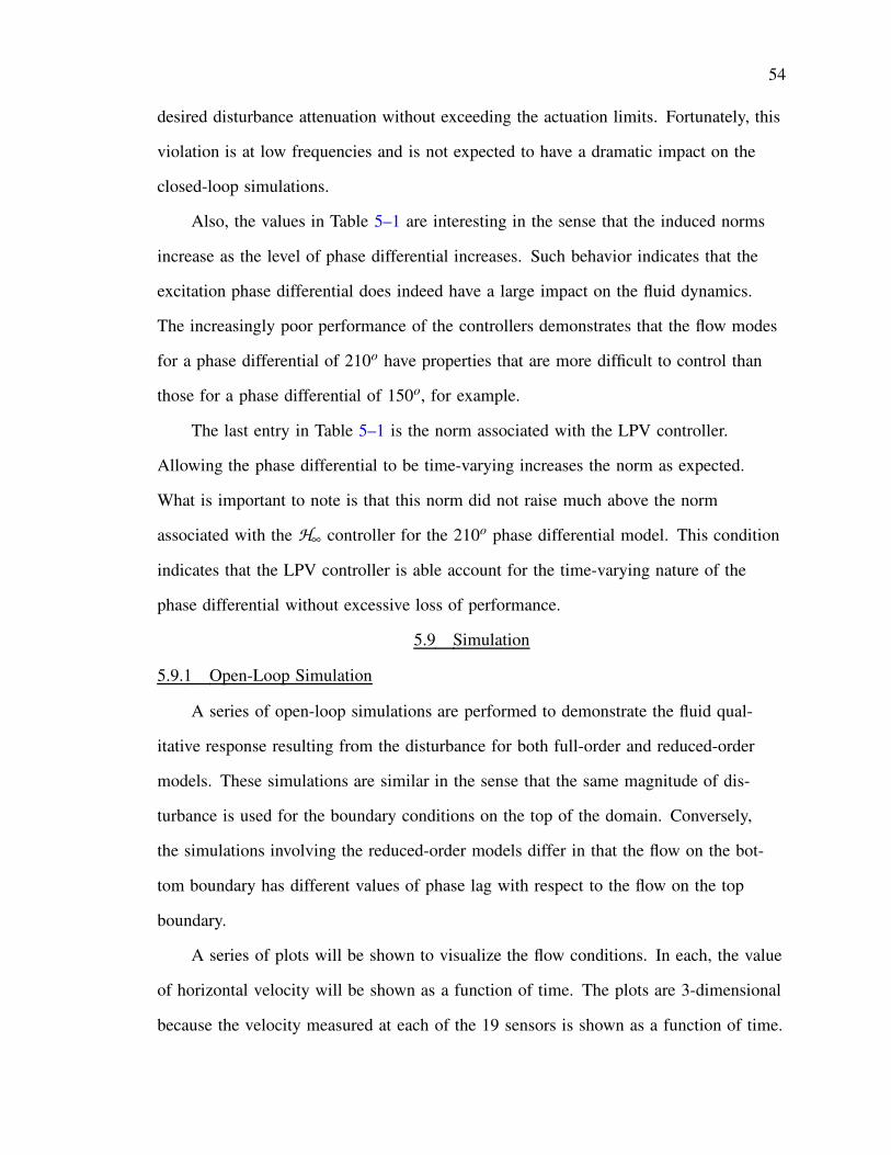
54
desired disturbance attenuation without exceeding the actuation limits. Fortunately, this
violation is at low frequencies and is not expected to have a dramatic impact on the
closed-loop simulations.
Also, the values in Table 5–1 are interesting in the sense that the induced norms
increase as the level of phase differential increases. Such behavior indicates that the
excitation phase differential does indeed have a large impact on the fluid dynamics.
The increasingly poor performance of the controllers demonstrates that the flow modes
for a phase differential of 210o have properties that are more difficult to control than
those for a phase differential of 150o, for example.
The last entry in Table 5–1 is the norm associated with the LPV controller.
Allowing the phase differential to be time-varying increases the norm as expected.
What is important to note is that this norm did not raise much above the norm
associated with the H∞ controller for the 210o phase differential model. This condition
indicates that the LPV controller is able account for the time-varying nature of the
phase differential without excessive loss of performance.
5.9 Simulation
5.9.1 Open-Loop Simulation
A series of open-loop simulations are performed to demonstrate the fluid qual-
itative response resulting from the disturbance for both full-order and reduced-order
models. These simulations are similar in the sense that the same magnitude of dis-
turbance is used for the boundary conditions on the top of the domain. Conversely,
the simulations involving the reduced-order models differ in that the flow on the bot-
tom boundary has different values of phase lag with respect to the flow on the top
boundary.
A series of plots will be shown to visualize the flow conditions. In each, the value
of horizontal velocity will be shown as a function of time. The plots are 3-dimensional
because the velocity measured at each of the 19 sensors is shown as a function of time.

55
Again, it is important to note that all measurements are non-dimensional. This
characteristic applies to both the time and velocity component so no units are noted for
the simulations.
The open-loop flow for the full-order model is used as a comparison for the
reduced-order model simulations (Figure 5–3). This plot clearly shows the sinusoidal
nature of the flow that results from the top exogenous disturbance changing with the
sine function, ho sin2πt . The flow near the center of the cavity, near point 11,
shows the largest velocity with a magnitude near -0.2 at t 03 to +0.2 at t 0
7.
0
0.5
1
510
1520
−0.2
0
0.2
TimePoint Index
Vel
ocity
Figure 5–3: Open-Loop Flow Velocities for Full-Order Model
The flow for the reduced-order model with a phase differential of 165o is shown
in Figure 5–4. This plot also demonstrates a sinusoidal nature, but has a smaller
open-loop magnitude compared to the full-order flow with the highest velocity being
0.07.
The flow for the reduced-order model with an phase differential of 210o is shown
in Figure 5–5. The flow again demonstrates a sinusoidal nature and the velocities are
slightly larger than those of the full-order model.
A sinusoidal trajectory of phase differentials shown in Figure 5–6 is used in a
simulation which shows the open-loop characteristics of the reduced-order flow as
phase differential changes.

56
0
0.5
1
510
1520
−0.2
0
0.2
TimePoint IndexV
eloc
ity
Figure 5–4: Open-Loop Flow Velocities for Reduced-Order Model with 165o PhaseDifferential
0
0.5
1
510
1520
−0.2
0
0.2
TimePoint Index
Vel
ocity
Figure 5–5: Open-Loop Flow Velocities for Reduced-Order Model with 210o PhaseDifferential
0 0.2 0.4 0.6 0.8 1150
160
170
180
190
200
210
Time
Phas
e D
iffe
rent
ial
Figure 5–6: Trajectory of Phase Differential

57
The flow velocities for the reduced-order model throughout the time-varying phase
trajectory are shown in Figure 5–7. The sinusoidal nature that is apparent in all of the
other open-loop flows is slightly different for this open-loop flow. This difference is
due to the changing of the parameter through the trajectory. The full-order flow does
not have a dependence on phase differential, therefore, the velocities for the full-order
model’s flow over the phase differential trajectory are the same as those plotted in
Figure 5–3.
0
0.5
1
510
1520
−0.2
0
0.2
TimePoint Index
Vel
ocity
Figure 5–7: Open-Loop Flow Velocities for Reduced-Order Model over a Trajectory ofPhase Differentials
An interesting feature to note is that the flow for each reduced-order model
with phase differential has a similar shape but significantly different magnitude. The
maximum velocity measured at the center of the cavity is smaller in magnitude for the
models with phase differentials located at the beginning of the range than the models
with phase differentials near the end of the range. This feature indicates the flow is
indeed strongly dependent on phase differential and should be considered for control
design.
5.9.2 Reduced-Order Closed-Loop Simulation
The closed-loop dynamics are also simulated to demonstrate the performance of
the controller for the reduced-order models, in this section, and the full-order model,
in the next section. The diagram of the closed-loop system for both the reduced-order

58
models and the full-order model can be seen in Figure 5–8. These simulations use the
same open-loop dynamics but include the linear parameter-varying controller that was
synthesized over the range of phase differentials, which contains 24 states. In each
simulation, the flow on the upper boundary is the same, but now the flow on the lower
boundary results only from the commands issued by the controller. In this section,
the controller was tested with reduced-order models for two specific cases of phase
differential and over a time-varying trajectory of phase differentials.
K '&h &
β Pδ & Ψ
R& Φα && Vm S
Figure 5–8: Closed-loop System
The measured velocities for the reduced-order model with a phase differential of
165o in response to the LPV controller with a phase differential of 165o is shown in
Figure 5–9. The comparison of these velocities with the open-loop measurements in
Figure 5–4 demonstrate a reduction of velocity along the center of the cavity, where the
velocity is greatest, of roughly 70%.
The measured velocities for the reduced-order model with a phase differential
of 210o in response to the LPV controller with a phase differential of 210o is shown
in Figure 5–10. The reduction in velocities is apparent by comparing the closed-loop
velocities in Figure 5–10 with the open-loop velocities in Figure 5–5, which shows a
reduction along the center of the cavity of roughly 90%.
The closed-loop simulation of the reduced-order models over the phase differential
trajectory, whcih also effects the controller, is shown in Figure 5–11. The velocity
magnitude shows a clear reduction in magnitude compared to the open-loop simulation

59
0
0.5
1
510
1520
−0.2
0
0.2
TimePoint IndexV
eloc
ity
Figure 5–9: Closed-Loop Flow Velocities for Reduced-Order Model with 165o PhaseDifferential
0
0.5
1
510
1520
−0.2
0
0.2
TimePoint Index
Vel
ocity
Figure 5–10: Closed-Loop Flow Velocities for Reduced-Order Model with 210o PhaseDifferential
of flow over the phase differential trajectory, which was shown in Figure 5–7. The
reduction along the center is roughly 80%.
The disturbance rejection is significant for the LPV controller with the reduced-
order models. These reductions confirm that the LPV controller will work not only
for reduced-order models at specific phase differentials but also over a time-varying
trajectory of phase differentials. The simulations did show some differences between
each of the reduced-order models. In particular, the amount of attenuation was slightly
less for the reduced-order model with a phase differential of 165o but much higher for
the reduced-order model with a phase differential of 210o. This decrease in attenuation

60
0
0.5
1
510
1520
−0.2
0
0.2
TimePoint IndexV
eloc
ity
Figure 5–11: Closed-Loop Flow Velocities for Reduced-Order Model over a Trajectoryof Phase Differentials
seems almost contradictory considering that the open-loop simulations showed a
decrease in flow velocities for the same models.
5.9.3 Full-Order Closed-Loop Simulation
The simulations that were performed for the reduced-order models were repeated
using the full-order model. The reduced-order models are subspaces of this full-order
model so the performance of the controllers on the full-order model is actually of
predominant interest.
The measured velocities in response to an H∞ controller, created specifically for
the full-order model, are shown in Figure 5–12. Clearly, the magnitude of the velocity
is dramatically decreased below the open-loop level. The velocities in Figure 5–12
are several orders of magnitude less than the corresponding open-loop velocities in
Figure 5–3. This response will be used as a comparison for the responses from the
full-order model controlled by the LPV controller.
The velocities for the full-order model in response to the LPV controller with a
phase differential of 165o is shown in Figure 5–13. Though the velocities were not
reduced to the extent of the full-order simulation in Figure 5–12, they were reduced
by an amount comparable to the response shown by the reduced-order model at a 165o
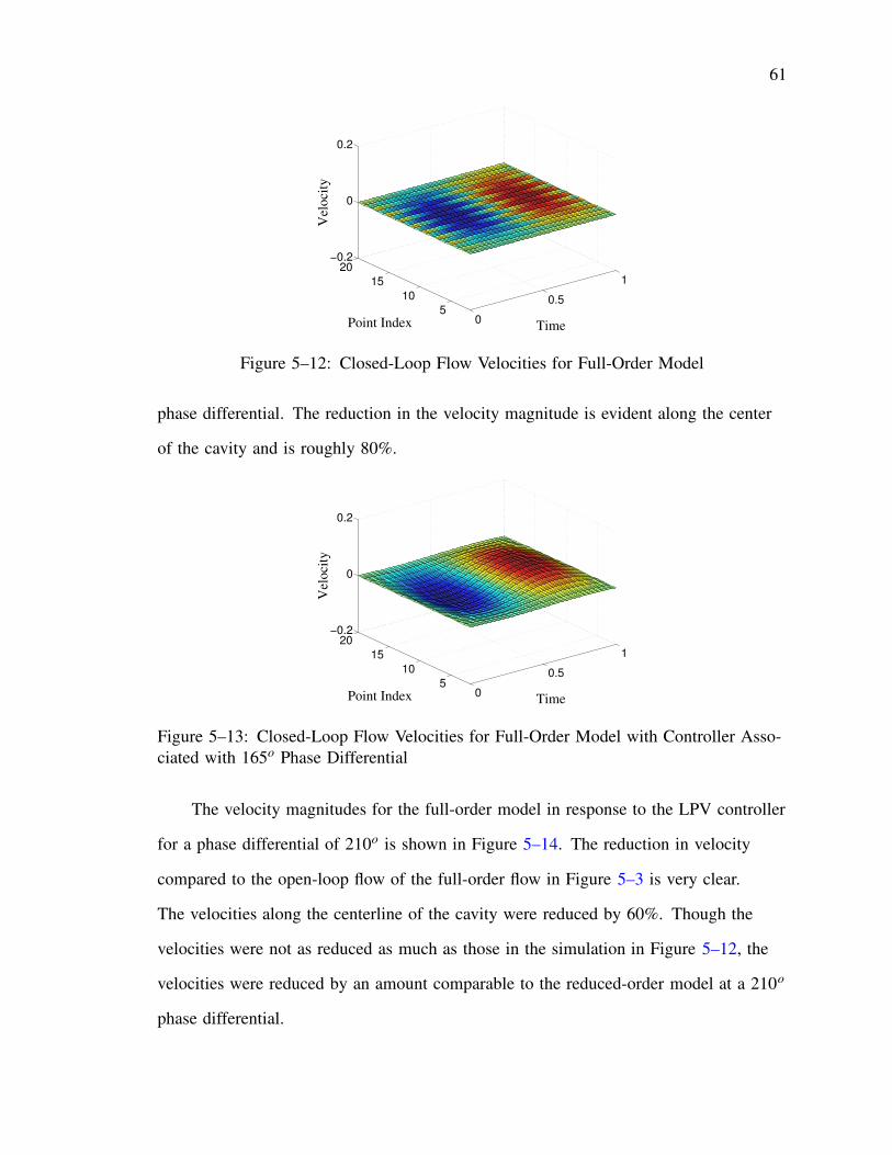
61
0
0.5
1
510
1520
−0.2
0
0.2
TimePoint IndexV
eloc
ity
Figure 5–12: Closed-Loop Flow Velocities for Full-Order Model
phase differential. The reduction in the velocity magnitude is evident along the center
of the cavity and is roughly 80%.
0
0.5
1
510
1520
−0.2
0
0.2
TimePoint Index
Vel
ocity
Figure 5–13: Closed-Loop Flow Velocities for Full-Order Model with Controller Asso-ciated with 165o Phase Differential
The velocity magnitudes for the full-order model in response to the LPV controller
for a phase differential of 210o is shown in Figure 5–14. The reduction in velocity
compared to the open-loop flow of the full-order flow in Figure 5–3 is very clear.
The velocities along the centerline of the cavity were reduced by 60%. Though the
velocities were not as reduced as much as those in the simulation in Figure 5–12, the
velocities were reduced by an amount comparable to the reduced-order model at a 210o
phase differential.

62
0
0.5
1
510
1520
−0.2
0
0.2
TimePoint IndexV
eloc
ity
Figure 5–14: Closed-Loop Flow Velocities for Full-Order Model with Controller Asso-ciated with 210o Phase Differential
The closed-loop simulation of the full-order model controlled by the LPV
controller over the phase differential trajectory is shown in Figure 5–15. The velocities
show a clear reduction in magnitude compared to the open-loop full-order flow in
Figure 5–3. The flow along the center of the cavity is reduced by 66%.
0
0.5
1
510
1520
−0.2
0
0.2
TimePoint Index
Vel
ocity
Figure 5–15: Closed-Loop Flow Velocities for Full-Order Model over a Trajectory ofPhase Differentials
The disturbance rejection is significant for both the reduced-order models and
the full-order model. These reductions confirm that the LPV controller, created for a
phase differential parameter, will work not only for the reduced-order models, which
are dependent on phase differential, but also for the full-order model.

63
5.10 Conclusion
Flow control is an exceedingly difficult challenge because of the nonlinearities
and time variations inherent to flow fields. These inherent difficulties can be avoided
when restricting the flow to creeping Stokes flow within a driven cavity. This project
has introduced a control methodology suitable for such a system. In particular, the
controllers are designed by considering subspaces of the flow field that describe modes
associated with phase differential between exogenous disturbances. The models of
these subspaces are realized as state-space systems and a controller can be designed
using the linear parameter-varying framework. The resulting controller is shown to
significantly decrease the flow velocities within the cavity for both the reduced-order
subspaces and also the full-order flow.
CHAPTER 6CONCLUSION
Practically all mechanical systems that involve motion need to be controlled with a
gain-scheduling technique. Aerospace systems in particular have the possibility to have
very extensive operating domains. Three specific aerospace systems were discussed in
this paper, the longitudinal dynamics of an
F/A-18, the structural dynamics of a hypersonic vehicle and the flow dynamics of a
driven cavity. The parameters that depicted the operating domain of the F/A-18 prob-
lem were altitude and Mach number. The parameter that depicted the operating domain
of the structure of the hypersonic vehicle was temperature and the operating domain
of the driven cavity was depicted by the phase differential within the fluid. This paper
has introduced a gain-scheduled control methodology, which uses H∞ synthesis to
create a linear parameter-varying controller, that is suitable for such systems. The LPV
controller created for the F/A-18 longitudingal dynamics proved to induce a pitch rate
for the aircraft that was similar to a designated target pitch rate. The LPV controller
created for the structural dynamics of a hypersonic aircraft successfully damped out
the vibrations induced by a temperature change. The LPV controller for the fluid
dynamics within a driven cavity significantly decreased the horizontal component of the
flow velocities along the centerline of the cavity for both the reduced-order subspaces
and the full order flow. The results of the control methodology to create proficient
controllers for three very different aerospace applications leads to the conclusion that
this methodology could be useful for other aerospace applications.
64

REFERENCES
[1] W. Rugh and J. Shamma, “Research on Gain Scheduling,” Automatica Vol. 36,Issue 10, John Hopkins University, Baltimore and UCLA, Los Angeles, October2000.
[2] D.J. Leith and W.E. Leithead, “Survey of Gain-Scheduling Analysis and Design,”International Journal of Control, Vol. 73, 2000, pp. 1001-1025.
[3] B. Bamieh and L. Giarre, “LPV Models: Identification for Gain SchedulingControl,” European Control Conference, 2001.
[4] L. Lee and M. Spillman, “Control of Slowly Varying LPV Systems: An Appli-cation to Flight Control,” AIAA Guidance, Navigation and Control Conference,AIAA-96-3805, 1996.
[5] J. Biannic, P. Apkarian and W. Garrard, “Parameter Varying Control of a HighPerformance Aircraft,” AIAA Guidance, Navigation and Control Conference,AIAA-96-3807, 1996.
[6] S. Bennani, D.M.C. Willemsen and C.W. Scherer, “Robust LPV Control WithBounded Parameter Rates,” Journal of Guidance, Control and Dynmaics, Vol. 21,No. 6, 1998, pp. 916-922.
[7] K. Tu and J.S. Shamma, “Nonlinear Gain-scheduled Control Design UsingSet-valued Methods,” American Control Conference, Vol. 2, 1998, pp. 1195-1199.
[8] J.S. Shamma and J.R. Cloutier, “Gain Scheduled Missile Autopilot Design UsingLinear Parameter Varying Transformations,” Journal of Guidance, Control andDynamics, Vol. 16, No. 2, 1993, pp. 256-263.
[9] R.A. Nichols, R.T. Reichert and W.J. Rugh, “Gain Scheduling for H-InfinityControllers: A Flight Control Example,” IEEE Transactions on Control SystemsTechnology, Vol. 1, No. 2, 1993, pp. 69-79.
[10] Z. Lin and M. Kammash, “Robust Gain-scheduled Aircraft Lontitudinal ControllerDesign using an H∞ Approach,” American Control Conference, 2001, pp. 2724-2729.
[11] S.M. Shahruz and S. Behtash, “Design of Controllers for Linear Parameter-Varying Systems by the Gain Scheduling Technique,” IEEE Conference onDecision and Control, Vol. 4, 1990, pp. 2490-2491.
65

66
[12] A. Sparks, “Linear Parameter Varying Control for a Tailless Aircraft,” AIAAGuidance, Navigation and Control Conference, AIAA-97-3636, 1997.
[13] L. Lee and M. Spillman, “Robust, Reduced-Order, Linear Parameter-VaryingFlight Control for an F-16,” AIAA Guidance, Navigation and Control Conference,AIAA-97-3637, 1997.
[14] R. Lind, J. Buffington, J. and A. Sparks, “Multi-loop Aeroservoelastic Controlof a Hypersonic Vehicle,” AIAA Guidance, Navigation and Control Conference,AIAA-99-4123, 1999.
[15] P. Gahinet and P. Apkarian, “A Linear Matrix Inequality Approach to H∞Control,” International Journal of Robust and Nonlinear Control, Vol. 4, 1995,pp. 421-448.
[16] J. Shin, “Optimal Blending Functions in Linear Parameter Varying ControlSynthesis for F-16 Aircraft,” American Control Conference, 2002, pp. 41-46.
[17] D. Malloy and B.C. Chang, “Stablilizing Controller Design for Linear ParameterVarying Systems Using Parameter Feedback,” AIAA Meeting Paper, AIAA-96-3808, July 1996.
[18] J. Mueller and G. Balas, “Impelmentattion and Testing of LPV Controllers forthe NASA F/A-18 Systems Research Aircraft,” AIAA Guidance, Navigation, andControl Conference, AIAA-2000-4446, 2000.
[19] P. Apkarian and P. Gahient, “Self-Scheduled H∞ Control of Missile via LinearMatrix Inequalities,” Journal of Guidance, Control and Dynamics, Vol. 18, No. 3,1995.
[20] G. Becker and A. Packard, “Robust Performance of Linear ParametericallyVarying Systems Using Parametrically-Dependent Linear Feedback,”Systems andControl Letters, Vol. 23, 1994, pp. 205-215.
[21] V. Verdult and M. Verhaegen, “Identification of Multivariable LPV State SpaceSystems By Local Gradiant Search,” European Control Conference, 2001,pp. 3675-3680.
[22] A. Nakajima and K. Tsumura, “Identification Methods for LPV MIMO Systems,”SICE Annual Conference, Vol. 2, 2002, pp. 1241-1245.
[23] M. Verhaegen and P. Dewilde, “Subspace Model Identification PartI: The Output-error State Space Model Identification Class of Algorithms,” International Journalof Control, Vol. 56, 1992, pp. 1187-1210.
[24] A. Kumar and M. Anderson, “A Comparison of LPV Modeling Techniques forAircraft Control,” AIAA Guidance Navigation and Control Conference, AIAA-2000-4458, 2000.

67
[25] F. Wu and A. Packard, “LQG Control Desgin for LPV Systems,” AmericanControl Conference, Vol. 6, June 1995, pp. 4440-4444.
[26] P. Apkarian, P. Gahinet and G. Becker, “Self-Scheduled H∞ Control of LinearParameter Varying Systems,” IEEE Conference on Decision and Control, Vol. 3,1994, pp. 2026-2031.
[27] P. Apkarian and P. Gahinet, “A Convex Characterization of Gain-Schedulede H∞Controllers,” IEEE Transactions on Automatic Control, Vol. 40, No. 5, 1995,pp. 853-864.
[28] R. Smith and A. Ahmed, “Robust Parmeterically Varying Attitude Controller De-sign for the X-33 Vehicle,” AIAA Guidance, Navigation and Control Conference,AIAA-2000-4158, 2000.
[29] R. Lind, “µ-Synthesis of an F/A-18 Controller,” AIAA Guidance, Navigation andControl Conference, AIAA-2000-4445, 2000.
[30] E. Jafarov and R. Tasaltin, “Design of Longitudinal Variable Structure FlightControl System for the F-18 Aircraft Model with Parameter Perturbations,” IEEEInternational Symposium on Computer Aided Control System Design, 1999,pp. 607-612.
[31] K.Tu, A. Sideris, K.D. Mease, J. Nathan and J. Carter, “Robust Lateral-DirectionalControl Design for the F/A-18,” AIAA Guidance, Navigation and ControlConference, AIAA-99-4204, Vol. 2, 1999, pp. 1213-1219.
[32] R. Lind, “Gain-Scheduled Approximations to H∞ Controllers for the F/A-18Active Aeroelastic Wing,” AIAA Guidance, Navigation and Control Conference,AIAA-99-4205, Vol. 2, 1999, pp. 1220-1230.
[33] G.J. Balas, J.B. Mueller and J. Barker, “Application of Gain-Scheduled Mul-tivariable Control Techniques to the F/A-18 System Research AIrcraft,” AIAAGuidance, Navigation and Control Conference, AIAA-99-4206, 1999.
[34] G.J. Balas, J.C. Doyle, K. Glover, A. Packard, and R. Smith, µ-Analysis andSynthesis Toolbox, The MathWorks, 2001.
[35] H. Buschek and A.J. Calise, “Fixed Order Robust Control Design for HypersonicVehicles,” AIAA Guidance, Navigation and Control Conference, AIAA-94-3662,1994.
[36] H. Buschek and A.J. Calise, “Robust Control of Hypersonic Vehicles ConsideringPropulsive and Aeroelastic Effects,” AIAA Guidance, Navigation and ControlConference, AIAA-93-3762, 1993.
[37] R. Lind, “Linear Parameter-Varying Modeling and Contol of Structural Dynamicswith Aerothermoelastic Effects,” Journal of Guidance, Control and Dynamics,Vol. 25, No.4, 2001, pp. 733-739.
68
[38] P. Vu and D.J. Biezad, “Longitudinal Control of Hypersonic Aircraft: An AlphaFollow-Up Scheme,” IEEE Regional Aerospace Control Systems Conference,1999, pp. 440-444.
[39] C.I. Marrison and R.F. Stengel, “Design of Robust Control Systems for aHypersonic Aircraft,” AIAA Guidance, Control of Dynamics Journal, Vol. 21,No. 1, 1998, pp. 58-63.
[40] Q. Wang and R.F. Stengel, “Robust Nonlinear Control of a Hypersonic Aircraft,”AIAA Guidance, Control and Dynamcis Journal, Vol. 23, No. 4, 2000, pp. 577-585.
[41] S.N. Balakrishnan, J. Shen and J.R. Grohs, “Hypersonic Vehicle TrajectoryOptimization and Control,” AIAA Guidance, Navigation and Control Conference,AIAA-97-3531, 1997.
[42] M. Sinai, “Hierarchical Design of Integrated Control for Hypersonic Vehicles,”IEEE Intelligent Control Symposium, Vol. 2, 1990, pp. 904-908.
[43] M. Heller, F. Hozapfel and G. Sachs, “Robust Lateral Control of HypersonicVehicles,” AIAA Guidance, Navigation and Control Conference, AIAA-2000-4248,2000.
[44] D.S. Naidu, S.S. Banda and J.L. Buffington, “Unified Approach to H2 and H∞Optimal Control of a Hypersonic Vehicle,” American Control Conference, Vol. 4,1999, pp. 2737-2741.
[45] F.R. Chavez and D.K. Schmidt, “An Integrated Analytical Aeropropul-sive/Analytical Model for the Dynamic Analysis of Hypersonic Vehicles,” AIAAAtmospheric Flight Mechanics Conference, AIAA-92-4567, 1992, pp. 551-563.
[46] D.K. Schmidt, H. Mamich and F.R. Chavez, “Dynamics and Control of Hyper-sonic Vehicles - The Integration Challenge for the 1990’s,” AIAA InternationalAerospace Planes Conference, AIAA-91-5057, 1991.
[47] F.R. Chavez and D.K Schmidt, “Analytical Aeropropulsive/AeroelasticHypersonic-Vehicle Model with Dynamic Analysis,” AIAA Guidance, Controland Dynamics Journal, Vol. 17, No. 6, 1994, pp. 1308-1319.
[48] F.R. Chavez and D.K. Schmidt, “Flight Dynamics and Control of Elastic Hyerp-sonic Vehicles: Modeling Uncertainties,” AIAA Guidance, Navigation and ControlConference, AIAA Paper 94-3629, 1994.
[49] J. Heeg, M.G. Gilbert and A.S. Pototzky, “Active Control of AerothermoelasticEffects for a Conceptual Hypersonic Aircraft,” Journal of Aircraft, Vol. 30, No. 4,July-August 1993, pp. 453-458.
[50] P. Gahinet, A. Nemirovski, A. Laub, M. Chilali, LMI Control Toolbox - UsersGuide, The MathWorks, Inc. Natick, MA, 1995.

69
[51] H. Chih-Ming, “Control of Fluid Flows by Micro Transducers,” IEEE Interna-tional Symposium on Micro Machine and Human Science, 1996, pp. 29-33.
[52] J. Ortiz and A. Barhorst, “Modeling Fluid-Structure Interaction,” Journal ofGuidance, Control and Dynamics, Vol. 20, No. 6, 1997, pp. 1221-1228.
[53] K. Ito and S.S. Ravindran, “A Reduced Order Method for Control of FluidFlows,” IEEE Conference on Decision and Control, Vol. 4, 1996, pp. 3705-3710.
[54] Y. Feng, A.J. Kurdila, R. Lind and D.W. Mikolaitis, “Linear Parameter-VaryingFlow Control for a Driven Cavity using Reduced-Order Models,” AIAA Guidance,Navigation and Control Conference, AIAA-2003-5351, 2003.
[55] J. Lumley, “The Structure of Inhomogeneous Turbulent Flows,” AtmopshericTurbulence and Radio Wave Propagation, edited by A.M. Yaglom and V.I.Tararsky, Nauka, Moscow, 1967, pp. 166-178.
[56] J.A. Burns and O. Yuh-Roung, “Feedback Control of the Driven Cavity ProblemUsing LQR Designs,” IEEE Conference on Decision and Control, Vol. 1, 1994,pp. 289-294.
[57] L. Baramov, O. Tutty and E. Rogers, “Robust Control of Linearized PoiseuilleFlow,” Journal of Guidance, Control and Dynamics, Vol. 25, No. 1, 2002,pp. 145-151.
[58] H.T. Banks, K. Ito, “Structural Actuator Control of Fluid/Structure Interactions,”IEEE Conference on Decision and Control, Vol. 1, 1994, pp. 283-288.
[59] O.K. Rediniotis, J. Ko, X. Yue, A.J. Kurdila, “Synthetic Jets, their Reduced OrderModeling and Applications to Flow Control,” AIAA Aerospace Sciences Meetingand Exhibit, AIAA-99-1000, 1999.
[60] S.S. Ravindran, “Reduced-Order Adaptive Controllers for MHD Flows UsingProper Orthogonal Decomposition,” IEEE Conference on Decision and Control,Vol. 3, 2001, pp. 2454-2459.
[61] L. Ji and J. Zhou, “The Boundary Element Method For Boundary Control of TheLinear Stokes Flow,” IEEE Conference on Decision and Control, Vol. 3, 1990,pp. 1192-1194.
[62] C.F.M. Coimbra and R.H. Rangel, “Spherical Particle Motion in Unsteady ViscousFlows,” AIAA Aerospace Science Meeting and Exhibit, 1999, AIAA-99-1031.
[63] K. Zhou, J.C. Doyle and K. Glover, “Robust and Optimal Control,” Prentice Hall,1st Edition, 1997.
BIOGRAPHICAL SKETCH
Kristin Fitzpatrick was born in Blue Hill, Maine on March 26, 1980. Her
family moved to Florida in 1988 after the death of her mother. She received her
high school diploma from the Center for Advanced Technologies, a magnet program
in St. Petersburg, Florida. She then attended the University of Florida and received a
degree in Aerospace Engineering with Honors in December 2002. She has worked with
the aerospace dynamics and control research group under the direction of Dr. Rick
Lind and Dr. Andy Kurdila and is projected to receive her Master of Science degree in
aerospace engineering in December 2003. She will stay at the University of Florida to
pursue a doctorate in aerospace engineering with the focus in dynamics and control.
70