U.S. Department of Transportation

Federal Highway Administration

Applications of Knowledge Discovery in Massive Transportation Data: The Development of a Transportation Research Informatics Platform (TRIP) PUBLICATION NO. FHWA-HRT-19-008 JANUARY 2019

Research, Development, and Technology Turner-Fairbank Highway Research Center 6300 Georgetown Pike McLean, VA 22101-2296

FOREWORD

Transportation researchers and practitioners have access to unprecedented amounts of data but lack the tools to easily store, manipulate, and analyze these data. The Transportation Research Informatics Platform (TRIP) is an informatics-based system designed to manage massive amounts of transportation data and provide researchers an efficient way to conduct analytics on big data. The objectives of TRIP include creating the ability to handle massive amounts of transportation data; utilize open-source technologies and tools to ingest, store, align, and process data; accept structured, semistructured, and unstructured datasets from any source; provide an efficient way to query data without indepth knowledge of metadata; integrate with open-source and consumer off-the-shelf analytics products; and provide visualization tools to offer greater insights into data. TRIP architecture is flexible and built on open-source state-of-the-art technology developed with big data in mind. Although predominantly developed for transportation safety research, TRIP is domain agnostic and capable of addressing issues pertaining to operations and maintenance given the ingestion of the appropriate datasets.

This document chronicles the development of the platform and provides background information on the need for analytical tools. In addition, this document supplies the resources and instructions on how to set up an instance of the platform and how to operate it. This document will be useful for transportation researchers, operators, and data managers interested in working with large transportation datasets.

Brian P. Cronin, P.E. Director, Office of Safety

Research and Development

Notice This document is disseminated under the sponsorship of the U.S. Department of Transportation (USDOT) in the interest of information exchange. The U.S. Government assumes no liability for the use of the information contained in this document.

The U.S. Government does not endorse products or manufacturers. Trademarks or manufacturers’ names appear in this report only because they are considered essential to the objective of the document.

Quality Assurance Statement The Federal Highway Administration (FHWA) provides high-quality information to serve Government, industry, and the public in a manner that promotes public understanding. Standards and policies are used to ensure and maximize the quality, objectivity, utility, and integrity of its information. FHWA periodically reviews quality issues and adjusts its programs and processes to ensure continuous quality improvement.

I

I I I

TECHNICAL REPORT DOCUMENTATION PAGE

1. Report No. FHWA-HRT-19-008

2. Government Accession No.

3. Recipient’s Catalog No.

4. Title and Subtitle: Applications of Knowledge Discovery in Massive Transportation Data: The Development of a Transportation Research Informatics Platform (TRIP)

5. Report Date January 2019 6. Performing Organization Code:

7. Author(s) Kevin Majka, Eric Nagler, Alex James, Alan Blatt, John Pierowicz, Panagiotis Ch. Anastasopoulos (ORCID: 0000-0002-1555-3308), Grigorios Fountas (ORCID: 0000-0002-2373-4221)

8. Performing Organization Report No.

9. Performing Organization Name and Address CUBRC 4455 Genesee St. Buffalo, NY 14225

10. Work Unit No.

11. Contract or Grant No. DTFH6115C00016

12. Sponsoring Agency Name and Address Office of Corporate Research, Technology, and Innovation Management Federal Highway Administration 6300 Georgetown Pike McLean, VA 22101

13. Type of Report and Period Final Report; April 2015–April 2018 14. Sponsoring Agency Code HRDS-2

15. Supplementary Notes James Pol (HRDS-2), Office of Safety Research and Development, served as the Technical Manager for the Federal Highway Administration. 16. Abstract Transportation researchers and practitioners have access to unprecedented amounts of data but lack the tools to easily store, manipulate, and analyze these data. The Transportation Research Informatics Platform (TRIP) is an informatics-based system designed to manage massive amounts of transportation data and provide researchers an efficient way to conduct analytics on big data. The objectives of TRIP include creating the ability to handle massive amounts of transportation data; utilize open-source technologies and tools to ingest, store, align, and process data; accept structured, semistructured, and unstructured datasets from any source; provide an efficient way to query data without indepth knowledge of metadata; integrate with open-source and consumer off-the-shelf analytics products; and provide visualization tools to offer greater insights into data. TRIP architecture is flexible and built on open-source state-of-the-art technology developed with big data in mind. Although predominantly developed for transportation safety research, TRIP is domain agnostic and capable of addressing issues pertaining to operations and maintenance given the ingestion of the appropriate datasets. 17. Key Words Informatics, analytics, big data, ingest, align, safety, operations, maintenance, visualization

18. Distribution Statement No restrictions. This document is available to the public through the National Technical Information Service, Springfield, VA 22161. http://www.ntis.gov

19. Security Classif. (of this report) Unclassified

20. Security Classif. (of this page) Unclassified

21. No. of Pages: 95

22. Price

Form DOT F 1700.7 (8-72) Reproduction of completed page authorized.

SI* (MODERN METRIC) CONVERSION FACTORS APPROXIMATE CONVERSIONS TO SI UNITS

Symbol When You Know Multiply By To Find Symbol

in ft yd mi

in2

ft2

yd2

ac mi2

fl oz gal ft3

yd3

oz lb T

oF

fc fl

lbf lbf/in2

LENGTH inches 25.4 millimeters feet 0.305 meters yards 0.914 meters miles 1.61 kilometers

AREA square inches 645.2 square millimeters square feet 0.093 square meters square yard 0.836 square meters acres 0.405 hectares square miles 2.59 square kilometers

VOLUME fluid ounces 29.57 milliliters gallons 3.785 liters cubic feet 0.028 cubic meters cubic yards 0.765 cubic meters

NOTE: volumes greater than 1000 L shall be shown in m3

MASS ounces 28.35 grams pounds 0.454 kilograms short tons (2000 lb) 0.907 megagrams (or "metric ton")

TEMPERATURE (exact degrees) Fahrenheit 5 (F-32)/9 Celsius

or (F-32)/1.8 ILLUMINATION

foot-candles 10.76 lux foot-Lamberts 3.426 candela/m2

FORCE and PRESSURE or STRESS poundforce 4.45 newtons poundforce per square inch 6.89 kilopascals

mm m m km

2mm 2m 2m

ha km2

mL L

3m 3m

g kg Mg (or "t")

oC

lx cd/m2

N kPa

APPROXIMATE CONVERSIONS FROM SI UNITS Symbol When You Know Multiply By To Find Symbol

mm m m km

2mm 2m 2m

ha km2

mL L

3m 3m

g kg Mg (or "t")

oC

lx cd/m2

N kPa

LENGTH millimeters 0.039 inches meters 3.28 feet meters 1.09 yards kilometers 0.621 miles

AREA square millimeters 0.0016 square inches square meters 10.764 square feet square meters 1.195 square yards hectares 2.47 acres square kilometers 0.386 square miles

VOLUME milliliters 0.034 fluid ounces liters 0.264 gallons cubic meters 35.314 cubic feet cubic meters 1.307 cubic yards

MASS grams 0.035 ounces kilograms 2.202 pounds megagrams (or "metric ton") 1.103 short tons (2000 lb)

TEMPERATURE (exact degrees) Celsius 1.8C+32 Fahrenheit

ILLUMINATION lux 0.0929 foot-candles candela/m2 0.2919 foot-Lamberts

FORCE and PRESSURE or STRESS newtons 0.225 poundforce kilopascals 0.145 poundforce per square inch

in ft yd mi

in2

ft2

yd2

ac mi2

fl oz gal ft3

yd3

oz lb T

oF

fc fl

lbf lbf/in2

* SI is the symbol for the International System of Units. Appropriate rounding should be made to comply with Section 4 of ASTM E380. (Revised March 2003)

ii

TABLE OF CONTENTS

CHAPTER 1. INTRODUCTION................................................................................................ 1 CHAPTER 2. PLATFORM COMPONENTS ........................................................................... 3

INFRASTRUCTURE SYSTEMS.......................................................................................... 3 DATA STORAGE AND DISTRIBUTION .......................................................................... 4 DATABASES AND SOURCES............................................................................................. 4 DATA INGEST, TRANSFORM, AND MANAGE ............................................................. 4 DATA PROCESSING, WAREHOUSING, AND QUERY................................................. 5 WEB CLIENT AND APP SERVER ..................................................................................... 5 ANALYTICS AND VISUALIZATION................................................................................ 6

CHAPTER 3. STUDY AREA AND DATA ................................................................................ 7 STUDY AREA......................................................................................................................... 7 DATA SOURCES ................................................................................................................... 8

HSIS ................................................................................................................................... 8 Clarus ................................................................................................................................. 8 RID ..................................................................................................................................... 9 Total Ingested Data........................................................................................................... 9

CHAPTER 4. RESEARCH QUESTIONS ............................................................................... 11 CHAPTER 5. ANALYTICS AND CAPABILITIES ............................................................... 15

CAPABILITIES.................................................................................................................... 16 UI ...................................................................................................................................... 18 Unified Data Models ....................................................................................................... 19 Visualization of Roadway Data 19 ...................................................................................... Entity Resolution............................................................................................................. 20 Dashboards ...................................................................................................................... 23 Visual Query Builder...................................................................................................... 23 SHRP2 NDS Time-Series Data ...................................................................................... 24 Benchmarking ................................................................................................................. 24 Safety Analyses................................................................................................................ 26

CHAPTER 6. PLATFORM SETUP AND USE....................................................................... 59 GENERAL CLUSTER SETUP........................................................................................... 59 WEB-SERVER SETUP........................................................................................................ 59 GEOSERVER SETUP.......................................................................................................... 60

Setting up the Database .................................................................................................. 60 Importing a GeoDB file into PostGIS ........................................................................... 61

TALEND OPEN STUDIO FOR BIG DATA ..................................................................... 62 JAVA, SCALA, AND WEB SOURCE CODE ................................................................... 64 JUPYTER NOTEBOOKS.................................................................................................... 65 ENTITY RESOLUTION...................................................................................................... 65 DASHBOARDING INSTALLATION................................................................................ 66 DATA CHARACTERIZER/LOADER .............................................................................. 67 UI2 INSTALLATION .......................................................................................................... 68 NGINX INSTALLATION.................................................................................................... 69

iii

USING TRIP ......................................................................................................................... 69 CHAPTER 7. SUMMARY......................................................................................................... 77 REFERENCES............................................................................................................................ 79

iv

LIST OF FIGURES

Figure 1. Graphic. TRIP components and typical workflow.......................................................... 3 Figure 2. Map. Demonstration area for TRIP ................................................................................. 7 Figure 3. Screenshot. TRIP UI...................................................................................................... 15 Figure 4. Screenshot. TRIP UI2.................................................................................................... 19 Figure 5. Screenshot. Visualization of roadway data ................................................................... 20 Figure 6. Chart. Server throughput ............................................................................................... 25 Figure 7. Chart. TRIP responsiveness .......................................................................................... 26 Figure 8. Graphic. Illustration of crash and noncrash data points ................................................ 27 Figure 9. Equation. Binary outcome probability for crash occurrence......................................... 29 Figure 10. Equation. Vectors of random parameters .................................................................... 30 Figure 11. Equation. V of random parameters .............................................................................. 30 Figure 12. Equation. Standard deviation of correlated random parameters ................................. 31 Figure 13. Equation. Standard error of the standard deviation for the correlated random

parameters ........................................................................................................................... 31 Figure 14. Equation. Computation of the t-statistic for the standard deviation of the

correlated random parameters ............................................................................................. 32 Figure 15. Equation. Correlation coefficient between two random parameters ........................... 32 Figure 16. Equation. Marginal effects of the explanatory variables............................................. 32 Figure 17. Equation. Density function of the conditional mean function..................................... 33 Figure 18. Equation. Ordered probit model formulation .............................................................. 33 Figure 19. Equation. Estimation of thresholds under the HOPIT framework .............................. 33 Figure 20. Equation. Probability of a crash resulting in j ............................................................. 34 Figure 21. Equation. Marginal effects for the explanatory variables of the ordered

probability model ................................................................................................................ 34 Figure 22. Equation. Probability that a crash will occur on a specific roadway segment, n,

in time, t, according to the random-parameters model estimated in phase 1 ...................... 35 Figure 23. Equation. Probability that a crash will occur on n in t according to the

correlated-grouped-random-parameters model ................................................................... 41 Figure 24. Equation. Probability that a crash will occur on n in t according to the

uncorrelated-grouped-random-parameters model ............................................................... 41 Figure 25. Equation. Likelihood ratio test statistic ....................................................................... 41 Figure 26. Equation. Probability of a crash resulting in no injury................................................ 48 Figure 27. Equation. Probability of a crash resulting in an injury................................................ 49 Figure 28. Equation. Probability of a crash resulting in a serious injury 49 ...................................... Figure 29. Equation. Probability of a crash resulting in a fatal injury.......................................... 49 Figure 30. Equation. Parametric function of the threshold between the no-injury and injury

outcomes.............................................................................................................................. 49 Figure 31. Equation. Parametric function of the threshold between the injury and serious-

injury outcomes ................................................................................................................... 50 Figure 32. Screenshot. Dynamically assigned crash risk.............................................................. 57 Figure 33. Screenshot. Talend Open Studio for Big Data home screen ....................................... 63 Figure 34. Screenshot. Talend with a data-load job...................................................................... 63 Figure 35. Screenshot. Jupyter notebook analysis ........................................................................ 65 Figure 36. Screenshot. TRIP welcome screen .............................................................................. 69

v

Figure 37. Screenshot. TRIP UI1.................................................................................................. 70 Figure 38. Screenshot. Time-range selector ................................................................................. 71 Figure 39. Screenshot. Text-search box........................................................................................ 71 Figure 40. Screenshot. Attribute-search tool ................................................................................ 72 Figure 41. Screenshot. Data source–attribute examiner ............................................................... 72 Figure 42. Screenshot. Query button with Geo Search option ..................................................... 73 Figure 43. Screenshot. Query results and attribute information ................................................... 73 Figure 44. Screenshot. Clarus weather station information.......................................................... 74 Figure 45. Screenshot. Base-layer selector ................................................................................... 74 Figure 46. Screenshot. NEXRAD imagery with time slider......................................................... 75 Figure 47. Screenshot. TRIP UI2.................................................................................................. 75 Figure 48. Screenshot. UI2 advanced visual query builder .......................................................... 76 Figure 49. Screenshot. Weather dashboard with traffic cameras.................................................. 76

vi

LIST OF TABLES

Table 1. Research questions, analytics, strategy, and output........................................................ 12 Table 2. TRIP phase 2 potential capabilities ................................................................................ 17 Table 3. GeoServer suite............................................................................................................... 20 Table 4. TRIP entity resolution—example 1 ................................................................................ 22 Table 5. TRIP entity resolution—example 2 ................................................................................ 22 Table 6. TRIP entity resolution—example 3 ................................................................................ 23 Table 7. Tabular illustration of crash stationary and dynamic information.................................. 27 Table 8. Descriptive statistics of key variables............................................................................. 35 Table 9. Model-estimation results................................................................................................. 36 Table 10. Model-estimation results for the correlated-grouped-random-parameters binary

logit model and its model counterparts ............................................................................... 39 Table 11. Diagonal and off-diagonal elements of the gamma matrix (t-stats in brackets) ........... 40 Table 12. Correlation coefficient matrix for the random parameters ........................................... 40 Table 13. Likelihood ratio test results........................................................................................... 42 Table 14. Distributional effect of the random parameters across observations............................ 42 Table 15. Marginal effects of the explanatory variables for the dynamic logit models ............... 43 Table 16. Descriptive statistics of key variables included in the injury-severity model .............. 47 Table 17. Model-estimation results for the HOPIT model ........................................................... 48 Table 18. Marginal effects of the explanatory variables for the HOPIT model ........................... 50 Table 19. Observed versus predicted crash and no-crash segments for the random-

parameters model estimated in phase 1 using the mean-β approach................................... 52 Table 20. Observed versus predicted crash and no-crash segments for the random-

parameters model estimated in phase 1 using the individual-β approach ........................... 53 Table 21. Observed and predicted crash and no-crash segments for the uncorrelated-

random-parameters model................................................................................................... 54 Table 22. Observed and predicted crash and no-crash segments for the correlated-grouped-

random-parameters model................................................................................................... 55 Table 23. Tomcat™ configuration................................................................................................ 59 Table 24. GeoServer suite............................................................................................................. 60 Table 25. TRIP subprojects........................................................................................................... 64 Table 26. Grafana™ setup parameters.......................................................................................... 66

vii

LIST OF ABBREVIATIONS AND SYMBOLS

Abbreviations

AADT annual average daily traffic API application programming interface CentOS Community Enterprise Operating System FHWA Federal Highway Administration FID feature identification code GDAL Geospatial Data Abstraction Library HDFS Hadoop Distributed File System HDP Hortonworks® Data Platform HOPIT hierarchical-ordered probit HSIS Highway Safety Information System NDS Naturalistic Driving Study NEXRAD Next Generation Radar npm node package manager ogr OGR Simple Features Library RAM random access memory RID Roadway Information Database RWIS roadway-weather information system sbt simple build tool SciPy Python scientific computing SHRP2 second Strategic Highway Research Program SPA single-page application SSL Secure Sockets Layer SQL Structured Query Language TRIP Transportation Research Informatics Platform UI user interface URI Uniform Resource Identifier YARN Yet Another Resource Negotiator

Symbols

AADTI annual average daily traffic per lane indicator ACCI access-control indicator ARBDI airbag-deployment indicator ADI alcohol/drugs indicator ADTL annual average daily traffic per lane CIn vector of the observable dynamic (variable over time for the same roadway

segment, and varying across roadway segments) characteristics associated with all possible discrete outcomes for roadway segment.

Cin vector of the observable dynamic (variable over time for the same roadway segment, and varying across roadway segments) characteristics that determine the crash occurrence for roadway segment.

cj vectors of estimable parameters

viii

Cor(xj,n,xn’,n) correlation coefficient between two random parameters cov(xj,n,xj’,n) CTI DGI E[P(yi)] HCI I i ICTH J j Ki

LCI LL(βd1) LL(βd2) 2 M M’ MCI MW N n P PI q P(y = 1) P(y = 2) P(y = 3) P(y = 4) Pn

RHI RI 𝑆𝑆𝑆𝑆𝜎𝜎𝑗𝑗 SGL SWI 𝑠𝑠𝜎𝜎 𝑗𝑗𝑗𝑗

t 𝑡𝑡𝜎𝜎𝑗𝑗 TVI V VCI VCLI VDI χ2

Xi

covariance between the two explanatory variables with random parameters collision-type indicator driver-gender indicator expected value of the mixed logit probability horizontal curve–length indicator set of all possible discrete outcomes of the crash occurrence. crash occurrence ice thickness or water depth on roadway surface highest injury-severity level integer ordered injury-severity level explanatory variable determining the thresholds of the ordered probit model lighting-conditions indicator log-likelihood function at convergence of the competitive dynamic model 1

log-likelihood function at convergence of the competitive dynamic models

probability function of the conditional mean function transposed function of the conditional mean function month-of-crash indicator median width number of observations used for model estimation roadway segment probability of an injury-severity level pedestrian indicator density function of the estimable parameters probability of no injury probability of injury probability of serious injury probability of fatal injury probability of crash occurrence for roadway segment relative-humidity indicator ramp indicator standard error of the standard deviation roadway-segment length shoulder-width indicator standard deviation of the observation-specific random parameter time t-statistic for the standard deviation of the correlated random parameter towed-vehicle indicator variance–covariance matrix vehicle-condition indicator vertical curve–length indicator vehicle’s direction indicator test statistic distributed with degrees of freedom equal to the difference in the number of explanatory parameters between the competitive models vector of explanatory variables

ix

XIn vector of the observable stationary (stable over time for the same roadway segment, but varying across roadway segments) characteristics associated with all possible discrete outcomes for roadway segment

Xin vector of the observable stationary (stable over time for the same roadway segment, but varying across roadway segments) characteristics that determine crash occurrence for roadway segment

xj,n explanatory variable with a random parameter (correlated with the parameter of xj’,n)

xj’,n explanatory variable with a random parameter (correlated with the parameter of xj,n)

yi integer corresponding to ordering of injury-severity outcomes zi unobserved dependent variable of the ordered probit model αj intercept for each threshold β mean value of the random-parameters vector β' transposed vector of estimable parameters βI vector of estimable parameters corresponding to all possible discrete outcomes βi vector of estimable parameters corresponding to crash occurrence βi vector of estimable parameters Γ symmetric matrix Γ΄ transpose of the symmetric matrix δi randomly distributed term with mean equal to 0 and variance equal to 1 εi random error term that is normally distributed with a mean of 0 and variance of 1 μ threshold parameter μ1 upper threshold for the injury outcome μ2 upper threshold for the serious injury outcome σj standard deviation of the random parameter σj,n standard deviation of the random parameter σj’,n standard deviation of the random parameter σk,1 off-diagonal element in the kth row and first column of the symmetric matrix σk,k respective diagonal element of the symmetric matrix σk,k−1 off-diagonal element in the kth row and (k−1)th column of the symmetric matrix σk,k−2 off-diagonal element in the kth row and (k−2)th column of the symmetric matrix φ vector of parameters of the density function corresponding to the estimable

parameters φ΄ density function of the standard normal distribution Φ cumulative function of the standard normal distribution

x

CHAPTER 1. INTRODUCTION

Great advancements have been made in transportation safety. However, motor-vehicle crashes are still a major cause of injuries and fatalities in the United States. Past innovative research has led to improvements in the design and safety of vehicles and roads, yet there is still much to be understood regarding the determination of factors, including driving behavior, that contribute to crashes. The second Strategic Highway Research Program (SHRP2) Naturalistic Driving Study (NDS) data enable innovative safety research to continue, but even though transportation researchers and practitioners now have access to an unprecedented amount of data, they lack the tools to easily store, manipulate, and analyze these data.(1)

One promising research area is informatics-based approaches to big-data analytics. Informatics pertains to the science behind making data accessible for knowledge discovery or mining, and analytics is the process used to discover patterns and meaningful information from data. The Transportation Research Informatics Platform (TRIP) is a complete informatics-based system designed to handle massive amounts and many forms of transportation data, provide researchers an efficient way to interact with data, and allow for the straightforward use of tools to analyze data. TRIP has been designed to be highly customizable and function with both legacy and innovative data stores. TRIP provides tools for researchers, enabling them to conduct big-data analytics in an efficient way. TRIP enables researchers to handle a wide range of transportation data on a scalable platform. TRIP can be deployed on a single workstation with a few megabytes of data or on a massive multinode distributed cluster with petabytes of data.

At its core, TRIP is based on Apache Hadoop™ technology, which allows TRIP to easily ingest, store, and process large amounts of data.(2) A data-retrieval layer based on PostgreSQL (SQL meaning Structured Query Language), GeoServer, and other Web services provides rapid access to data; the handling of contextual, temporal, and geospatial searches; and the ability to quickly serve the data to transportation safety researchers.(3,4) Finally, the main user interface (UI) is designed as a Web application so that TRIP can be easily deployed and accessed.

The initial design requirements specified that TRIP would be deployed to analysts to conduct transportation-safety research based on the integration of the Highway Safety Information System (HSIS), the SHRP2 Roadway Information Database (RID), and Clarus data within the Seattle, WA region.(5–7) The research team envisions that TRIP could be deployed at U.S., State, and local transportation departments and other transportation-related facilities, such as metropolitan planning organizations and traffic incident management and operations centers. The overall architecture of TRIP, which was built on all open-source, state-of-the-art technologies and developed with big data in mind, is flexible. The overall design goals for TRIP included the following abilities:

• Handle massive amounts (e.g., terabytes) of transportation data.• Utilize open-source technologies and tools to ingest, store, align, and process data.• Accept structured, semistructured, and unstructured datasets from any source.• Provide an efficient way to query data without indepth knowledge of metadata.• Integrate with open source and consumer off-the-shelf products.• Visualize data to provide greater insights and understanding.

1

To accomplish the design goals, seven process layers were built: infrastructure systems; data storage and distribution; database and sources; data ingest, transform, and management; data processing, warehousing, and query; analytics and visualization; and Web-clients and application server. Generally, each layer is dependent on the layers that precede it. Each of the process layers has been tested at various stages of development through the use of agile development practices and unit testing. Major components are iterated for multiple development cycles to create features and remove bugs. The components are then unit tested individually for functionality and completeness. In addition, experiments have been conducted on the system components and validated through the use of research queries.

In order to demonstrate the functionality of the overall system, several user access points and interfaces were developed. TRIP utilizes a modern, streamlined, Web-based UI for remote access and query capabilities. The UI provides basic analytics and visualization through the use of an interactive, visual query builder and data characterizer and viewer. These analytics provide access to temporal, categorical, and spatial queries as well as visualization of the datasets and linkages. Temporal queries can be performed by selecting desired time frames that are continuous or segmented by hours of interest. The categorical search tool allows analysts to select attributes of interest through an indexed data characterizer; thus, they do not require indepth knowledge of the source metadata. The spatial-query tool enables interactive selection of specific locations through the use of an on-screen display. The results and attributes are made instantly available in a separate data window. The unified UI provides the ability to view HSIS crash information, RID roadway data, along with the closest Clarus weather data (both time and space) and Next Generation Radar (NEXRAD) imagery from the Iowa Environmental Mesonet.(5–8)

The capabilities of TRIP can be extended and customized to users’ needs by providing linkages to many popular analytics packages, such as R, SAS®, MathWorks® Matlab®, Microsoft® Excel™, etc. As an example of a linkage between TRIP and a analytics package, and to provide a demonstration of the full potential of the platform, Jupyter notebooks were used in this study.(9)

Notebooking technology enables analysts to collect and run code, provide text descriptions and visualizations, and develop and test models all in one place. Analysts also have to ability to import a rich set of libraries with previously designed algorithms or models that can be customized and executed against the full set of data ingested in the platform. Finally, as another extension, dashboarding capabilities have been included as a rapid way to summarize and visualize streaming and historical data. Specific examples have been developed that provide summary reports on crash information along with supplemental weather and traffic camera data in graph and tabular forms.

The development of a full-scale prototype has allowed for integration testing of individual components of TRIP. Proven functionality and validity of results have been established through various demonstrations throughout the development of the platform. In addition, a task to benchmark the platform has been completed to test the components in an integrated way. Validation of the functionality of the components was performed through the execution of 10 queries that relied on the interoperability of the process layers. The following chapters of this report provide detailed descriptions of the platform components, the study area and data, the research questions used to validate and test the platform, included analytics and capabilities, platform setup and use, and finally, a summary and conclusions.

2

Formulate Question

Collect Data

Transform Data

Analyze Results

Present Results

Infrastructure Systems

Storage and Distribution

Databases and Sources

Ingest, Transform, and Manage

Process, Warehouse, and Query

Web Client and App Server

Analytics and Visualization

,n

cu 8 -·-cu C: C a,

en

,n C:

..... 2 C: -(1) cu ·- 0 o= Q!

Q! ~

CHAPTER 2. PLATFORM COMPONENTS

TRIP development focused on designing and building a big-data analytics platform to handle the diverse types of information the Federal Highway Administration (FHWA) collects and analyzes. TRIP allows an analyst to collect, transform, analyze, and publish results for others to consume. This chapter provides the documentation relevant to the specific components of TRIP. TRIP was designed to be readily available to transportation research, planning, and operations agencies and is built on open-source, state-of-the-art technology. The key components of the platform and the associated tasks of a typical workflow are illustrated in figure 1.

© 2017 CUBRC.

Figure 1. Graphic. TRIP components and typical workflow.

INFRASTRUCTURE SYSTEMS

The foundation of the infrastructure-systems layer consists of the hardware and operating systems that power this analytics platform. The infrastructure-systems layer contains both the servers hosting the data and analytics and the client machines accessing the server resources. The servers run a distribution of the Linux operating system.(10) The distribution chosen is Community Enterprise Operating System (CentOS).(11) CentOS has a large community-based support. Using such a distribution encourages long-term support and stability for TRIP. The dedicated commodity servers, which hold and process the data for this platform, are dual Xeon processor servers with 128 gigabytes of random access memory (RAM) and six 2-terabyte hard drives. This hardware setup and operating system offers a flexible environment for client

3

machines to access the server resources. Client machines simply need to be able to run a modern Web browser.

DATA STORAGE AND DISTRIBUTION

The data-storage and -distribution layer enables TRIP’s processing and storage capabilities. To handle the current and future volume of data the platform is expected to process, a Hadoop™ framework is employed.(2) The Hadoop™ framework consists of multiple subprojects, each focusing on one component of an entire big-data solution. When Hadoop™ is installed on a collection of systems, which is called a cluster, a specific distribution of Hadoop™ that guarantees all components of the Hadoop™ ecosystem are tested and validated to appropriately work with each other needs to be chosen. TRIP employs the Hortonworks® distribution of Hadoop™, called Hortonworks® Data Platform (HDP).(12) To provision and install HDP, the built-in provisioning tool called Apache Ambari™ was used.(12,13) Ambari™’s responsibility is to provision, manage, and monitor clusters running Hadoop™.(13,2)

The two major components that HDP provides are the Hadoop™ Distributed File System (HDFS) and Yet Another Resource Negotiator (YARN).(12,2) The HDFS is the main storage location for files to be queried and analyzed. When files are placed in the HDFS, portions of the files called blocks are distributed throughout the cluster. A block size is typically either 64 or 128 megabytes. These blocks are then replicated, by default, three times across the nodes of the cluster. This process enables fault tolerance across the cluster, meaning if one machine holding these data fails, then the data are still accessible.

The Hadoop™ YARN negotiator enables running applications to request processing resources from the cluster.(2) Each node of the machine has processing resources that can be allocated to running applications. When the application is started, it will request the cluster resource manager to run. A unit of these cluster resources is called a container. A container is usually defined by the amount of RAM requested for it. An entire application is defined by the number of containers requested.

Usually, when an application starts, it requests resources like 4 containers with 2 gigabytes of RAM each or 16 containers with 4 gigabytes of RAM each. YARN will then attempt to fulfill the request and start the application. If the request cannot be fulfilled, then YARN will suspend the application and wait until the amount of resources requested can be fulfilled. Due to this dynamic allocation ability, YARN can run and optimize multiple types of workflows. Long-running applications can be started and left running to a batch analysis, and real-time applications can accept requests for data and publish results to Web services.

DATABASES AND SOURCES

A detailed description of the data sources is provided in chapter 3.

DATA INGEST, TRANSFORM, AND MANAGE

After launching the data platform, the first step was to ingest the data sources into the Hadoop™ data lake.(2) A data lake is a centrally managed repository for big data. There are two main methods to manage a data lake. The first method is to use Talend Open Studio for Big Data, a

4

visual extract, transform, and load tool.(14) Talend is capable of taking data from a large variety of data sources and transforming and loading them into the target data store. Talend supports a wide range of file formats, database types, and vendors. The second method utilizes Apache Hive™ to manually transfer, store, and manage the schema of the data.(15) Hive™ is a data warehousing system built on top of Hadoop™, allowing individuals to manage tabular-based data sources.(15,2) Hive™ enables SQL queries to be run against Hadoop™, which bypasses the need to learn how to query against Hadoop™ natively.(15,2) An alternative method is to copy the files directly to the HDFS. This method is acceptable if the data are guaranteed to have an error-free schema.

DATA PROCESSING, WAREHOUSING, AND QUERY

To enable scaled-out distributed processing, an Apache Spark™ framework was employed.(16)

Spark™ enables high-performance distributed processing for big-data applications. Spark™ has a variety of different methods for accessing the underlying data stored in the HDFS. One method is via the native access application programming interface (API) and the second is via the SQL API. For the applications written, both APIs were used to retrieve and process the underlying data. Spark™ applications can be written in Java, Scala, Python, and R. Along with these processing capabilities, one interesting feature of Spark™ is its support of in-memory processing. With Spark™, a dataset can be promoted to memory, allowing for operations to be performed much quicker compared to accessing the information on disk.

Spark™ enables large, scaled-out analytics queries but does not offer instant data access.(16) To enable this process, Apache HBase™ is utilized.(17) HBase™ is an open-source, key-value, distributed database written on Hadoop™.(17,2) A key-value database has one indexed column that can be queried for instant data access. The database is also distributed among multiple nodes for fault-tolerance and query scalability. For the demonstrated UI, the crash data are loaded into HBase™ and queried from the Web client to be displayed on the Web UI.(17) For optimal query capability, sometimes the data are duplicated multiple times in different tables or representations to enable the fastest queries possible, depending on what the user requests.Along with Spark™ and HBase™ for large-scale, distributed analytics, PostgreSQL and PostGIS are utilized for real-time data access and geospatial indexing. (See references 16, 17, 3, and 18)

WEB CLIENT AND APP SERVER

A Web application was created to interact with and display analyzed data. This Web client has the ability to query and filter data, display results on a map, and perform natural text searches for locations. To enable these features, a handful of technologies were used on the client (Web browser) side and the server side.

To enable a rich user experience, the Google® Angular Web-application framework was used.(19)

The Angular 2 framework was created by Google® to create a single-page application (SPA). An SPA is different from a traditional Web application in that, in a traditional Web application, pages are served one at a time from a server, whereas when an SPA loads, the entire Web application is downloaded from the service and run in the Web browser. This feature of SPAs eliminates the need to load pages one at a time from the server and provides a quicker and more responsive user experience overall. Along with Angular 2, a handful of plug-ins were utilized.

5

Leaflet was used as TRIP’s open-source geospatial visualization framework.(20) Leaflet supports a variety of basemaps (OpenStreetMap®, MapQuest®, ESRI®, etc.) and offers customizable layers and markers.(20–23) Geometry information can be stored in PostgreSQL, but to publish and visualize that information, GeoServer is used.(3,4) GeoServer is an open-source server designed to read and serve geospatial data from a variety of sources.(4) GeoServer can produce data in Web feature service, Web map service, and Keyhole Markup Language formats among a variety of others. Similarly, information can be read into GeoServer in shapefile formats, such as PostGIS, GeoTIFF, and MrSID.(4,18) A listing of all of the formats can be found on the GeoServer documentation page.(24)

The application server used is Apache Tomcat™.(25) Tomcat™ is an open-source Java servlet container allowing for Java-based applications to be served to clients. In this container, applications are developed using a combination to two Web-application frameworks, Scalatra and Oracle® Jersey.(26,27) Scalatra is a Web-application microframework that permits Web applications to be developed quickly with minimal overhead.(26) It was modeled after the Sinatra framework for creating Web applications. Jersey is mainly used with Atmosphere, which is for creating and using websockets in the application.(27,28) A websocket offers persistent connections between the server and client without the overhead of reestablishing a new connection each time.

ANALYTICS AND VISUALIZATION

A detailed description of the analytics tools is provided in chapter 5 of this document.

6

Pierce County

-~ Suliona

- RIO Ortttn Roactw•~ I King Pieree. Snohomish County

CHAPTER 3. STUDY AREA AND DATA

This chapter provides a description of the study area and data that were selected to demonstrate the capabilities of TRIP, although the platform itself is agnostic to geographic boundaries.

STUDY AREA

To demonstrate the ability of TRIP to process and combine disparate datasets and return novel information, a study area surrounding Seattle, WA, was selected. The Seattle area was chosen for the following reasons: Seattle (specifically, King, Pierce, and Snohomish Counties) was one of the larger SHRP2 NDS data-collection sites, RID data were collected to support the NDS in the Seattle area, multiple active and reporting roadway-weather information system (RWIS) stations were archived in the Clarus system, and Washington State has participated in the HSIS data-sharing program. (See references 1, 6, 7, and 5.) In addition, during the phase 2 effort of SHRP2 NDS, data collected in the Seattle test site area, including time-series data, annotated video data, and driver-assessment information, were also available.(1) Figure 2 illustrates the study area that was examined in the TRIP project and displays the 4,277 mi of centerline data available in RID and the 27 RWISs located in the 3-county area.(6)

© 2017 CUBRC.

Figure 2. Map. Demonstration area for TRIP.

7

DATA SOURCES

As part of the initial development and demonstration effort, TRIP supports and hosts a sample of data from the Seattle, WA, region from HSIS, Clarus weather data, SHRP2 RID, and NEXRAD weather imagery from the Iowa Environmental Mesonet. (See references 5, 7, 6, and 8.) Utilizing these four data sources will enable the research team to demonstrate a number of important capabilities of TRIP, including the ability to handle large amounts of data and process queries across multiple databases.

HSIS

HSIS is a comprehensive database of crash records and detailed roadway information maintained by FHWA. Currently, California, Ohio, North Carolina, Illinois, Maine, Minnesota, and Washington actively contribute to HSIS.(5) Previously, Michigan and Utah also provided data to HSIS. The databases include information on crashes of differing severity levels; traffic volumes; as well as characteristics of intersections, curve/grade, and interchange facilities. The differences in State data-collection systems and resulting variation in reported data provide an opportunity for TRIP to demonstrate its ability to function across databases through the use of a common data model. The following is a summary of HSIS data size:

• Data for King, Pierce, and Snohomish Counties in Washington State from 2011 to 2013. • Eight tables, which contain a total of 202,073 records and 83,074,533 cell values, of data. • Uncompressed file storage size of 129 megabytes.

A data request was made to HSIS for a complete set of data for King, Pierce, and Snohomish Counties in Washington State from 2011 to 2013.(5) A complete list of metadata available for Washington State is available on the HSIS website.(29)

Clarus

In order to monitor weather throughout the United States, there are approximately 2,175 automated weather sites (typically at airports), including 879 automated surface observing systems, 20 automated weather sensor systems, and 1,276 automated weather observing systems. In addition, there are over 2,000 RWIS sites. The Clarus Initiative was an effort to provide complete information on atmospheric-weather and roadway-surface conditions in real time for over 4,000 locations throughout the United States.(7,30) In many cases/locations, the data were archived for further analysis. Recently, the Clarus system, which was operated by FHWA, was transitioned to the Meteorological Assimilation Data Ingest System, which is operated by the National Oceanic and Atmospheric Administration. These detailed and microscopic weather data offer new opportunities to support transportation research from safety and operational perspectives. The following is a summary of Clarus data size:

• Data for all stations in the State of Washington from 2011 to 2013. • 14 tables, which contain a total of 59,109,128 records and 6,967,164,174 cell values. • Uncompressed file storage size of 6.45 gigabytes.

8

A data request was made to FHWA for a complete set of archived Clarus data for King, Pierce, and Snohomish Counties in Washington State from 2011 to 2013.(7) This request was processed and data were received for all Clarus stations in the entire State of Washington for that time period. A complete list of metadata available for the archived Clarus data is available online through FHWA’s website, Weather Data Environment.(31)

RID

RID was created as part of SHRP2.(6) To create RID, an instrumented vehicle was driven on the roads on which SHRP2 NDS participants at each of the six test sites (including the Seattle, WA, test site) most frequently drove.(1) RID contains detailed information on roadway geometrics and attributes for more than 12,500 centerline-mi of roadway. In addition, it contains information on roadway infrastructure as well as supporting historical data on crashes, weather, traffic laws, safety campaigns, and work zones obtained from State transportation departments. Data are available for roadways within and surrounding the SHRP2 NDS study center test sites, which include Buffalo, NY; Seattle, WA; Tampa, FL; Raleigh–Durham, NC; State College, PA; and Bloomington, IN.(1) The following is a summary of RID data size:

• Entire database, minus the video log for Washington State. • 66 tables, which contain a total of 3,719,870 records and 1,962,156,038 cell values. • Uncompressed file storage size of 3.57 gigabytes.

A complete list of metadata available for RID is available online through Iowa State University’s Center for Transportation Research and Education website.(6)

Total Ingested Data

The following is a summary of the total data size:

• 88 tables containing a total of 60,031,071 records and 9,012,394,745 cell values. • Uncompressed file storage size of 10.15 gigabytes. • After ingestion into TRIP, the total file storage size utilized is 5.03 gigabytes.

9

CHAPTER 4. RESEARCH QUESTIONS

This chapter identifies the research areas that were selected in order to test and validate the capabilities of TRIP as well as offer examples of the types of queries that will be possible. These queries illustrate the unique capabilities of this approach and the power of leveraging massively large datasets for analysis. Although predominantly developed for transportation-safety research, TRIP is domain agnostic and capable of addressing issues pertaining to operations and maintenance given the ingestion of the appropriate datasets.

TRIP provides safety analysts the ability to develop dynamic statistical models that have the capability to identify hazardous locations or hot spots in terms of the number of crashes by injury severity and in terms of the likelihood of crash occurrence. This capability allows for the prediction of the risk of a transportation-network user being involved in a crash as a driver, passenger, pedestrian, or transit user and for the prediction of the risk of a specific vehicle being involved in a crash. Furthermore, the identification of hazardous locations and crash-risk forecasts for vehicles and users can be used to provide equitable resource allocation to effectively preserve the transportation network and improve the network’s safety performance. Safety analysts can then make informed recommendations to develop or improve engineering, enforcement, or education solutions.

Table 1 illustrates the possible types of queries within TRIP that are specific to the ingested datasets. These research questions represent the types of questions that can be answered via TRIP but are not exhaustive. The technical descriptions and answers provided are meant to be illustrative of the tools and techniques that have been built into TRIP, not definitive answers to a select few research questions. In addition to the research questions, table 1 also shows the requirements and data needed to answer each question, the implementation strategies, the necessary tools and analytics, and the overall status of each question.

These examples rely on attributes of incorporated datasets, their relationships, as well as derivative information. TRIP has the ability to ingest common data sources and supports the use of natural language queries. Ontological representations of time of day, temperature, and age of driver can be defined and represented in order to answer the posited questions. An additional benefit of TRIP is the ability not only to make these queries, but to make them across nonstandardized databases in an efficient manner.

11

12

Table 1. Research questions, analytics, strategy, and output. Database

(6,7,5)No. Research Parameters Analytics Initial Implementation Strategies Status 1 Identify all crashes where it

was freezing for less than 1 h on roadways that have one travel lane and are undivided.

RID, Clarus Spatial distance, weather, road exposure over distance (modeling)

1.

2.

Collect the set of roadways that have one travel lane and are undivided; collect crashes on these roadways. Collect spans of time that it was freezing for less than 1 h. Need to generate spans of time and pick the leading edge of the line chart.

Compl ete: A map identifies all crashes with c onditions in which it was freezin g for less than 1 h on roadways that ha ve one travel lane and are undivi ded. Travel lanes were not identif ied; therefore, this solution identif ies all roadways that meet only the other parameters.

3. Merge both datasets, and output crashes.

2

3

Identify all run-off-the-road crashes on undivided, curved, two-lane, rural roads within 1 h of reported snow and or rain conditions.

What roadway types had the greatest percentage increase in serious-injury crashes over the last 3 yr, separated out by urban rural classification?

RID, Clarus

RID, HSIS

Weather, proximity

Aggregation

1.

2.

3.

4. 1.

2.

3.

Retrieve the set of run-off-the-road crashes matching the question’s criteria. Collect time spans that it was freezing for less than 1 h. Determine the overlap of the time spans using a sliding, adjustable window to account for hourly and location differences. Display results back to the user. Aggregate and apply a simple filter on the data. Output a table grouped by roadway characteristics and crash types. Provide a count of serious

Incom plete: This question is unsup ported by the data received. Roadw ay-surface temperatures are missin g for a significant number of locatio ns. An example of joining roadw ay surface temperatures to crashe s could be provided, but it will not pr ovide statistical significance. Additi onal data will be required to proceed.

Compl ete: Bar plots and tables provide results to this question. Greatest increa se (8.9%) was on urban, two-way, l eft-turn lanes.

crashes. 4 In what type of weather are

pedestrians more likely to be involved in a crash?

RID, HSIS Aggregation 1.

2.

Collect the set of crashes in which pedestrians were involved. Aggregate information on weather year by year, and visualize it as a bar graph.

Complete: Histogram and mosaic plots identify that clear or partly cloudy, overcast, and raining have the largest magnitudes, respectively. Normalization would be an important additional step.

Database (6,7,5)No. Research Parameters Analytics Initial Implementation Strategies Status

13

5 What roadway curvature characteristics present an increased risk factor for commercial vehicles?

6 What locations, as a function of traffic volume and clear weather conditions, exhibit a higher-than-expected crash risk?

7 What makes and models of vehicles are more likely to be involved in crashes of which speeding was a causal factor?

8 Do snow-covered roadways lead to increased single-vehicle, run-off-the-road

RID Stacked box plots, machine-learning model

1.

2.

3.

Determine how to retrieve a crash with a commercial vehicle. Retrieve that set of crashes and retrieve the curvature information associated with that crash. Plot the roadway curvature characteristics versus the all of the crashes, and stack the same

Complete: Overall, with a combination of roadway-curvature characteristics and event-based crash data can provide many different opportunities to gain insights using a variety of different analytics-visualization and -training techniques. Three different models were invoked to return results for this question. They include a decision tree, a random forest, and a k-

plot on top of the roadway condition information.

nearest neighbor model.

4. Attempt to model the crash types using the curvature characteristics as the source of information.

5. Select several different machine

RID, HSIS, Clarus

RID

HSIS

Aggregation, traffic-volume function, level of service

Aggregation

Aggregation, comparison

1.

2.

1.

2.

3.

1.

learning–model types as the basis for evaluation, and report performance of those models. Create a model that takes in weather and AADT and makes a prediction of the probability of a crash. Research needs to be done on this front. Input different locations, and output a percentage from 0 to 1. Find reports that indicate that speeding was a factor. Create a dataset that combines roadway and crash information with speed limits. Aggregate makes and models, and output a table. Capture the range of daylight hours for a period of time.

Incomplete: This question is unsupported by the data received. Traffic volumes are missing for a significant number of locations. Additional data will be required to proceed.

Complete: Histograms provide results indicating that, for the RID dataset, the Honda Civic is the most popular vehicle and for HSIS the Toyota SXC is the most popular vehicle.

Complete: Histograms and pie charts show that the most popular contributing factors for dry conditions are other and over centerline. For

Database No.

9

10

Research Parameters crashes on curves during daylight hours?

Is crash severity correlated to roadway-surface temperature?

Find all senior drivers who struck pedestrians at intersections with crosswalks but without pedestrian-crossing lights during twilight hours.

(6,7,5)

HSIS, Clarus

HSIS, RID

Analytics

Correlation measure, roadway-temperature interpolation

Entity resolution

Initial Implementation Strategies 2. Find single-vehicle run-off-the-

road crashes that occur on snow-covered roadways.

3. Categorize the crashes and group the results.

1. Compile a dataset of crash severities paired with roadway-surface temperatures.

2. Determine an appropriate correlation measure to use, and apply it to the data.

3. Return the correlation measure.

1. Find when twilight was for the time range of interest.

2. Retrieve an oversized sample of drivers (age greater than 40) who struck pedestrians with the defined parameters.

3. Allow user to select age and output a table.

Status winter-like conditions, the most popular are exceeding reasonable and safe speed and over centerline.

Incomplete: This question is unsupported by the data received. Roadway-surface temperatures are missing for a significant number of locations. An example of joining roadway-surface temperatures to crashes could be provided, but it will not provide statistical significance. Additional data will be required to proceed. Complete: Tables provide results of the 25 crashes that met the criteria in HSIS and for the 45 crashes recorded in RID.

Event Validation Criteria: Time of Event, Vehicle Heading, Speed Limit

14

AADT = annual average daily traffic.

0T.,,..R.w,gto

• •

>_ Tensearcn

Detailed Information for Accident: E228841

Oat11 Soo1ce RID

... g•IICl•r

,n1,NUn4k 12200'°'57Nl10)01 ... =::•UftOMOtG

.-Ill

Multiple Data Sources

CHAPTER 5. ANALYTICS AND CAPABILITIES

Basic analytics are available to the analyst through the use of the Web-based UI illustrated in figure 3. These analytics provide temporal, categorical, and spatial queries as well as visualization of the datasets and linkages.

© 2017 CUBRC; Basemap © 2017 MapQuest.

Figure 3. Screenshot. TRIP UI.(22)

The temporal query allows analysts to select desired time frames that can be continuous or sliced or segmented by hour(s) of interest (e.g., morning peak or day(s) of the week). The categorical-search tools allow the analyst or researcher to select attributes of interest from the crash databases. The spatial-query tools support the identification of specific locations and their corresponding crashes. In addition to the query portion of the UI, a display of results and attributes is instantly made available to the analyst. From this window, additional information associated with crashes from alternative datasets is also available. For instance, crash information from both RID and HSIS can be viewed along with the closest (in time and space) Clarus weather data.(6,5,7) In addition, some advanced features that are under development include radar-intensity data and the ability to step through a passing weather-event time using a time slider.

Advanced analytics generate insights into data that enhance the richness of the output by exploiting targeted aspects of the data. TRIP is designed with these capabilities in mind. TRIP includes core resolution analytics for entity and event resolution that feature the ability to customize attribute sets that are required for reliable entity coreference and disambiguation. Unlike many other approaches to coreference resolution, the TRIP approach applies probabilities of shared feature sets to entities to assert whether one entity is the same as another. This functionality is reliable within documents, across documents, and even across data sources. An added bonus to this approach is that social-network algorithms can execute against all data

15

sources as entity resolution will prune out duplicate entities without over-populating a network graph.

TRIP was designed to provide great flexibility to analysts and researchers. As such, linkages have been provided to many popular analytics packages and tools that allow users to develop methodologies and strategies for their analyses. Many of these packages contain built-in libraries with algorithms or models for analyses. The current implementation of these tools occurs within the Jupyter notebooks section of TRIP with the intent of providing integration into the Web-based UI.(9)

Jupyter notebooks are Web pages that enable the combination of code, visualization, and word processing all in one document.(9) With a Jupyter notebook, algorithms and visualizations can be prototyped quickly and easily and then shared with colleagues. Later, the code or algorithmic process written can be transitioned to running applications to power front-end applications. Some of the tools used to enable analytics and visualization include scikit-learn (machine-learning library), Pandas (data-manipulation tool), and Folium (map plotting tool).(32–34)

The Python scientific computing (SciPy) tool stack was selected for the development of customizable analytics within the platform. The SciPy tool stack is free, open source, and well documented; it also has a large development community.(35) Just like Hadoop™, Python comes in a variety of distributions.(2) For this platform, the Anaconda distribution was chosen for its large variety of prebuilt, commonly used Python software packages and ease of use.(36)

Along with Python-based tools, there are a handful of other analytical tools available for use in TRIP.(35) Apache Zeppelin™ is a new notebooking tool for big data.(37) Zeppelin™ primarily uses Spark™ for analytics, whereas Jupyter notebooks support many additional programming languages.(37,16,9)

CAPABILITIES

This section describes the capabilities that were developed for the current iteration of TRIP. A list of requirements and potential capabilities was developed in order to evaluate which offered the most potential value to users. Table 2 identifies each enhancement, its focus area, whether the task is dependent on accomplishing another task, the estimated level of effort (in labor weeks) needed to accomplish the enhancement, an average ranking determined by FHWA and the project team, and if the enhancement would be included in phase 2.

16

Table 2. TRIP phase 2 potential capabilities. LOE Phase 2

# Enhancement Focus Area Dependency (Week) Rank Selection 1 Expanded UI capabilities Systems None 2 2.2 Yes 2 Benchmarking Systems None 2 4.6 Yes 3 Data security Systems None 2 8.7 No 4 Containerization of apps Systems None 2 19.0 No 5 Safety analyses Analytics #10 4 4.0 Yes 6 Contextual associations Systems None 16 8.0 No 7 Cross tables (data cubes) Analytics #8 8 11.3 No 8 Unified data models (forms) Analytics None 8 4.3 Yes 9 More like these (queries) Analytics None 12 10.7 No 10 Visualization of roadways Visualization None 4 5.7 Yes 11 Thematic mapping Visualization 2 part 12 16.0 No 12 Hot-spot and density mapping Visualization #10, #11 16 14.0 No 13 Drawing and annotation Visualization None 8 18.5 No

capabilities 14 SHRP2 NDS time-series data(1) Data None 4 4.0 Yes 15 Social media (Twitter™) Data None 12 16.0 No 16 V2V/V2I communications Data None 12 12.0 No 17 Volume/congestion data Data #10 8 11.0 No 18 Expanded geographic coverage Data None 4 9.5 No 19 Integrating streaming data Data None 12 11.0 No

sources 20 Dashboards Systems #19 4 13.7 Yes 21 Visual query builder Systems #7, #8 12 8.5 Yes

V2V = vehicle to vehicle; V2I = vehicle to infrastructure; LOE = level of effort.

17

The following capabilities were selected to be included in phase 2:

• Expanded UI capabilities. • Benchmarking. • Highway Safety Manual-type safety analyses.(38)

• Unified data models. • Visualization of roadway data. • SHRP2 NDS time-series data.(1)

• Dashboards. • Visual query builder.

UI

The phase 1 TRIP UI (version 1) allowed users to run a limited number of queries against a backend Web service and display the results on a map. The UI did not, however, provide complete access to all of the tools available in the notebooking interface. Expanding the UI to include the following elements would make improve the overall user experience:

• Provide interactive geosearching. • Retrieve a crash by identifier. • Export query results to a .csv (comma-separated values) file. • Aggregate single-time and time-range bundles. • Save, load, and share queries to different users.

To develop the UI’s advanced capabilities, the map-browser and visual-query-builder modules were separated into two distinct interfaces. The separation of these interfaces optimizes the map-viewing and -querying experience.

• The map-browser module enhancements include more basemaps, orthoimagery, and the ability to display all types of vector layers (point, line, polygon) on the map.

• The visual-query-builder module permits the construction of complex queries in a network format with the ability to be executed against multiple target databases.

In addition, enhancements to the UI to support other tasks performed were also developed and are illustrated in figure 4. All components have been rigorously tested to ensure functionality.

18

© 2017 CUBRC; Basemap © 2017 MapQuest.

Figure 4. Screenshot. TRIP UI2.(22)

Unified Data Models

To optimize the visual query builder’s capabilities, a common data model was necessary. The development of TRIP in phase 1 did not have a single centralized data model for accessing data. This circumstance made it difficult to consistently query the data. Leveraging the work done in phase 1, the different schemas were unified into one centralized data model while maintaining the source provenance. This unified data model facilitated the extraction of information and reduced the complexity of the developed systems. This model allowed for a more intuitive and efficient query interface in UI2 and provided better data characterization. To support the unified data models, the following components of UI2 were adjusted or modified:

• Data characterization was improved to maintain provenance of data sources, which can be visualized in UI2.

• Entity-resolution code was improved to facilitate the addition of more field comparators and grouping functions.

• Geolocation storage was improved so that geolocations are now stored in a database that allows for spatial query and extraction.

Visualization of Roadway Data

The visualization capability supports the drawing of roadway segments and networks as editable layers in the platform. In order to accomplish this task, GeoServer was setup on the TRIP server.(4) Utilizing GeoServer and the associated suite of tools listed in table 3, the roadway data from RID, which is in geodatabase format (.gdb), were imported into PostGIS using the Geospatial Data Abstraction Library (GDAL) “ogr2ogr” command.(18,39) GeoServer affords TRIP

19

• ifr1 Tlan~RHNf'thlnfonn1tk.•PI.Mfotm O WCMM p au.y

.., __ □-□ ---□ -"­□-□-□-□ M<-

□-□-□ ...

increased spatial-query capabilities and enhances the ability and efficiency to view spatial data.(4,6)

Table 3. GeoServer suite.(4)

Tool Name PostgreSQL(3)

PostGIS(18)

Version 9.5 2.2

Description/Use Relational database backend to hold data and geometries. PostGIS supports geographic objects.

pgAdmin Ⅲ©(40)

1.22.1 Administration tool for PostgreSQL.

GDAL(39) 2.1.1 GDAL is a computer software library for reading and writing

GeoServer(4) 2.9.1 raster and vector geospatial data formats. Connects to and serves geo tiles and data.

Similar to the point data that have already been incorporated, it is now possible to query, identify (i.e., view attribute data), and stylize roadway data (represented by lines). Figure 5 is an illustration of simple roadway data overlaid on a basemap in version 2 of TRIP’s UI.

© 2017 CUBRC; Basemap © 2017 MapQuest.

Figure 5. Screenshot. Visualization of roadway data.(22)

Entity Resolution

Entity resolution allows an analyst to quickly perform a comprehensive search and collect important attributes of that entity automatically. The process begins with some defining information about an entity of interest, such as a crash. The entity resolution algorithm then searches the data sources based on the provided information and finds other mentions of that entity, some of which will contain additional attributes not previously known to the analyst (e.g., crash causation, make and model of vehicle). These additional attributes are collected and aggregated into a more complete representation of the crash’s true attributes. The resulting

20

visualization may present this information as a table of crash attributes, as a timeline of important events, or as a map of the location of the crash.

The approach to entity resolution taken in TRIP is modeled after an equality logic problem. This model operates using only strong identifiers or a set of attributes that collectively behave as strong identifiers (e.g., crash report number, time, and location). Attributes that behave as strong disidentifiers, meaning they contain conflicting information, are used to detect inconsistencies with the strong identifier models. When a conflict in strong identifiers occurs (e.g., two crashes occurred at the same location but at different times), an attempt will be made to resolve this in the way most likely to reflect reality. Unlike many other approaches to probabilistic data linkage, the research team’s approach applies probabilities of shared feature sets to entities to assert whether one entity is the same as another. This functionality is reliable within documents, across documents, and even across data sources.

The entity resolution capability demonstrated for the TRIP project is a proof-of-concept algorithm that adapts principles from the more mature data-association algorithm that runs on the Hadoop™ platform.(2) For the sake of demonstration, the capability to identify and aggregate descriptions of the same crash but sourced from different databases (i.e., HSIS and RID) was developed.(5,6) No single attribute is unique to a crash in both sources, and aggregating attributes from both databases yields more information than is available from either source by itself. To demonstrate the ability of the algorithm to function on a larger problem set, only weakly identifiable attributes were utilized to correlate crashes. For example, a strong identifier, such as the location of the crash, was not used; however, combination sets, such as time of crash, vehicle make, and driver gender, were. Overall, a set of 13 attributes was combined with appropriate similarity comparison transforms to associate approximately 99.6 percent of crashes identified in HSIS with records in RID.(5,6)

Table 4 through table 6 compare attributes of three sets of crashes. Each row is given a weighted value based on how well the records match. For two records to be associated, the aggregated score must be above a user-selected threshold. The records in table 4 match because there is enough similarity to associate them; the records in table 5 are a possible match because several attributes match, but they do not have a high enough aggregate score to be associated; an evaluation of the records in table 6 indicates these records do not match.

21

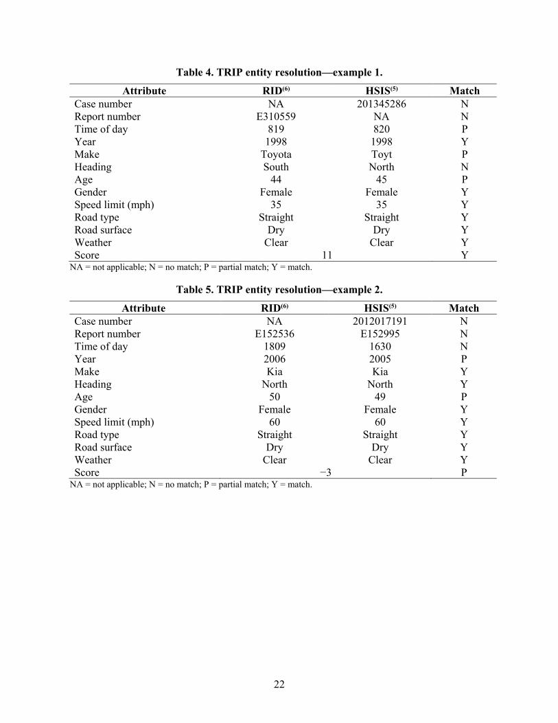
Table 4. TRIP entity resolution—example 1.

Attribute RID(6) HSIS(5) Match Case number NA 201345286 N Report number E310559 NA N Time of day 819 820 P Year 1998 1998 Y Make Toyota Toyt P Heading South North N Age 44 45 P Gender Female Female Y Speed limit (mph) 35 35 Y Road type Straight Straight Y Road surface Dry Dry Y Weather Clear Clear Y Score 11 Y

NA = not applicable; N = no match; P = partial match; Y = match.

Table 5. TRIP entity resolution—example 2.

Attribute RID(6) HSIS(5) Match Case number NA 2012017191 N Report number E152536 E152995 N Time of day 1809 1630 N Year 2006 2005 P Make Kia Kia Y Heading North North Y Age 50 49 P Gender Female Female Y Speed limit (mph) 60 60 Y Road type Straight Straight Y Road surface Dry Dry Y Weather Clear Clear Y Score −3 P

NA = not applicable; N = no match; P = partial match; Y = match.

22

Table 6. TRIP entity resolution—example 3.

Attribute RID(6) HSIS(5) Match Case number NA 201345286 N Report number E162518 E16003 N Time of day 145 1828 N Year 1995 2010 N Make Honda Niss N Heading West Northeast N Age 19 56 N Gender Female Male N Speed limit (mph) 55 60 N Road type Straight Straight Y Road surface Dry Wet N Weather Clear Raining N Score −11 N

Dashboards

Dashboards are centralized places that provide an at-a-glance view of information. The main TRIP UIs (versions 1 and 2) are primarily query-based systems and do not provide the capability to continuously run analytics in the background or provide updates over time. Dashboards enable analysts to develop queries (new crashes matching certain criteria, such as current weather conditions, etc.) and display the results in real time from streaming data with alerts, notifications, maps, charts, or graphs. To provide an example of this functionality within the allotted development time, a version of this technology that relies on ingested data rather than streaming data and is static rather than providing updated information in real time was developed.

The TRIP dashboard module has two main components. The first component is Grafana™, which is a dashboarding Web application designed to create metric and analytic dashboards.(41)

It enables query and visualization from multiple data sources and the ability to create summary charts, graphs, and tables from data. The second component is InfluxDB, which is a time series– sequenced database.(42) This temporal data structure is used because it optimizes querying and display over a time dimension. Although the demonstrations show archived historical crash data, they can be adjusted to show real-time local traffic, incident-detection sensors, weather information, air-quality data, and other relevant time-based information with relatively modest additional development focused on provided connectors to external streaming data.

Visual Query Builder

The first version of TRIP’s UI contained a simplified way to query attributes but did not approach the complexity that is possible within the notebooking interface. A novice user should be able to build complex queries within the Web UI and have a visual way to document his/her selection. To meet these needs, an advanced interactive visual query builder was developed, which allows analysts to select and drag different variables and operators into a window and then connect them in a logical way to create complex queries.

23

In order to support the new capabilities required in the advanced visual query builder, PostgreSQL and PostGIS technologies were employed.(3,18) PostgreSQL is an open-source, relational database allowing for storage of relational, tabular-based data.(3) PostGIS is a plug-in for PostgreSQL allowing for geospatial analytics to be run on top of PostgreSQL’s relational model.(18,3) This architecture offers a variety of geospatial analytics and functions to be run against the geometry data. These tools also provide the ability to transform the RID ESRI® geodatabase file (.gdb) to PostgreSQL allowing for query access outside of ArcGIS™.(6,3,23)

Overall, the visual query builder improves the query capabilities of TRIP UI version 2. To develop the advanced capabilities and include them in the UI, the map browser and query modules were modified. The components were separated into two distinct interfaces that can be viewed side by side, resized, and minimized independently. The separation of the map browser from the query module presents the opportunity to focus on building the best interface possible for map viewing and querying, respectively. The map browser–module enhancements include more basemaps, orthoimagery, and the ability to display all types of vector layers (point, line, polygon) on the map. The query-builder module permits the construction of complex queries in a network format with the ability to be executed against multiple target databases. To support the advanced features, two new technologies were utilized for network display and graphing. These technologies were Almende B.V. vis.js for the visualization of the query network and Chart.js for the visualization of data histograms.(43,44)

SHRP2 NDS Time-Series Data

The purpose of this task was to demonstrate the ability to ingest a large amount of SHRP2 NDS time-series data and integrate it with the search methods built into the platform.(1) A fundamental feature of TRIP is the ability to work with large amounts of data, and therefore, the time-series data certainly represent a sufficiently large dataset that benefits from the built-in data-handling features to query, associate, and extract information. Having an easy way to associate the time-series data with RID data and detailed weather information is also advantageous.(6) To demonstrate the ability to incorporate SHRP2 NDS time-series data, a sample dataset of trips was requested.(1) These trips have been made available for view and query within the platform and can be overlaid with other ingested layers, including RID data and time-specific weather information.(6)

Benchmarking

Evaluating the speed of backend analysis and measuring the ability of the Web interface to scale to multiple users were the two means of benchmarking TRIP the research team used. Benchmarking began by recording an interaction sequence using the TRIP UI. Once recorded, the load-testing software Apache JMeter™, which replayed the session as if multiple simulated users were simultaneously using TRIP, was utilized.(45) To vary interactions, the recorded sequence was edited to focus on specific technical aspects of TRIP (e.g., one sequence utilized aerial imagery whereas another sequence did not).

Two attributes of the system, server throughput and responsiveness, were captured to describe system performance. To measure server throughput, a range of 1–60 simultaneous users was simulated. As illustrated in figure 6, the system provided a consistent amount of throughput

24

" C: 0 u Q) V,

~

100

~ 10 V,

t;; Q) ::, Cj' Q)

a::

1

. ' Target Benchmark

0 10

Server Throughput

' 20 30 40 50

# of Users

~ w/ MrSID, Server Throughput w/o MrSID, Server Throughput - Web UI API

60

regardless of the number of users. The exception to this finding was when users requested aerial imagery. An initial analysis indicated that the decrease in throughput is due to the additional processing required to decompress the aerial imagery. Spreading imagery across multiple servers would likely increase throughput if there were a large number (over 30) of simultaneous users.

In the case of server responsiveness, the average amount of time taken for the server to provide requested data was measured. Then, the standard deviation of response times was computed and plotted over the number of simulated users. For cases of fewer than 60 simultaneous users, the responsiveness of TRIP (regarding both UI elements and data requests) was well within accepted ranges (figure 7). Similar to the first measure, when aerial imagery is utilized, the server can reasonably support 30 simultaneous users before a noticeable decrease in responsiveness occurs. Again, distributing the imagery across several servers would likely mitigate this issue in a production context.

© 2017 CUBRC.

Figure 6. Chart. Server throughput.

25

....... c~

100%

Q _g 90% ta ~ ~ ~ 80%

7Cf'/4

60%

50%

4Cf'/4

3Cf'/4

2Cf'/4

lCl'/4

0%

Server Responsiveness

Target Benchmark with Imagery _______ _

___________ Target Benchmark with out Imagery ...

0

-----10 20 30 40

# of Users

--+- w/ MrSID > .25 std .dev --<r- w/ MrSID > 0.5 std.dev

w/o MrSID > .25 std.dev --- w/o MrSID > .5 std.dev

50 60

© 2017 CUBRC.

Figure 7. Chart. TRIP responsiveness.

Safety Analyses

To predict potential hazardous locations (hot spots) in time and space, the dynamic binary random (mixed) parameters probit/logit model was employed. To that end, dynamic data elements were linked with stationary information, and crash-occurrence probabilities were identified. The output was the likelihood that a crash will occur on a specific roadway segment in a specific time interval.

The dynamic data elements included the following:

• Weather information (e.g., temperature, rain precipitation, snow precipitation, and other weather-specific information).

• Pavement-surface condition.

The stationary data elements included the following:

• Roadway geometrics (e.g., number of lanes, horizontal- and vertical-curvature characteristics, median and median-barrier characteristics, and shoulder information).

• Roadway functional characteristics (e.g., roadway classification, controlled access, and speed limit).

26

.4.ccidam

Segment - 11 5 I I i ldQ. /.,-30 lo T1II1e (I)

Accident Segment - 337

I I i l;;;;§.Q 1-30 T=e (I)

.4.ccidem

Segment - 665

L --{)0 1,-30 t, Tnne (I)

• Average traffic characteristics (e.g., annual average daily traffic (AADT) and trafficcounts for single units).

The data were aggregated over 30-min intervals from the moment that a crash occurred. Note that the data were available for a 1-h period before the moment that a crash occurred. Figure 8 illustrates three data points (over the two 30-min intervals) in graphic format. Table 7 displays the way the stationary and dynamic information is arranged in the dataset in a tabular format.

© 2017 CUBRC. to = time of the crash occurrence for segment – 115; t = time of the crash occurrence for segment – 337; t1 = time of crash occurrence for segment – 665; to–30 = 30 min before the time of the crash occurrence for segment – 115; t–30 =30 min before the time of the crash occurrence for segment – 337; t1-30 = 30 min before the timeof the crash occurrence for segment – 665; to–60 = 60 min before the time of the crash occurrence for segment– 115; t–60 = 60 min before the time of the crash occurrence for segment – 337; t1–60 = 60 min before the timeof the crass occurrence for segment – 665.

Figure 8. Graphic. Illustration of crash and noncrash data points.

Table 7. Tabular illustration of crash stationary and dynamic information.

t = time of the crash occurrence; t–30 = 30 min before the time of the crash occurrence; t–60 = 60 min before the time of the crash occurrence.

27

The data do not only include roadway segments where crashes have occurred, but also roadway segments without crashes along with the corresponding stationary and dynamic elements of all segments for the time intervals described in the previous paragraph. This consideration contributes to efficiently capturing the influence of dynamic elements on crash-occurrence probabilities of a roadway segment.

The implemented approach supports the identification of dynamic elements that may lead to a crash while controlling for stationary elements, such as road geometrics and traffic characteristics. Therefore, the focus of the safety analyses lies in identifying precrash dynamic factors using extremely disaggregate information, as compared to the traditional approach, which looks at stationary factors using aggregated data. The main benefit of the implemented approach is that, in addition to the factors that play in the traditional crash-occurrence analysis, it accounts for dynamic elements that are neglected in the traditional approach.

The identification of potential hazardous locations is associated not only with the crash occurrence, but also with the injury-severity outcome of a possible crash. On the basis of the stationary and dynamic data elements, the injury severity–outcome probabilities can also be identified. To investigate the precrash and at-crash determinants of the injury-severity outcomes, a hierarchical ordered probability framework was employed. The output was the likelihood that a crash would result in a specific injury-severity outcome. In addition to the set of stationary and dynamic data elements that are used for the crash-occurrence analysis, the injury-severity analysis leverages a broad range of crash-specific information, such as the following:

• Driver-specific characteristics (e.g., age, gender, license status, driving experience, sobriety level, and consciousness level).

• Vehicle-specific characteristics (e.g., vehicle type, model, make, age, and pre- and postcrash condition).

• Collision-specific characteristics (e.g., collision type, major contributing factors, ejection status, lighting conditions, and environmental conditions).

• Injury-severity information (e.g., most severe injury observed and number of injured persons).

Methodological Framework In the statistical analysis of phase 1, a dynamic binary random (mixed) parameters probit/logit model is estimated. This model accounts for the dynamic nature of the dynamic explanatory parameters as well as the possibility of random variations in parameters across observations that can cause serious specification problems that could result in inconsistent parameter estimates and outcome probabilities. To that end, the binary (1 for crash occurrence and 0 otherwise) outcome probabilities can be written as shown in figure 9.

28

e</J;X;.+/JiC;,)

Pn(i I (f)) = J :~::e(/JiX1>,+/J,C1>,) q(fi I (f))d fi

'!fl

Figure 9. Equation. Binary outcome probability for crash occurrence.

Where: n = roadway segment. i = crash occurrence. I = set of all possible discrete outcomes of i. φ = vector of parameters of the density function corresponding to the estimable parameters. Pn = probability of crash occurrence for n. Xin = vector of the observable stationary (stable over time for the same roadway segment,

but varying across roadway segments) characteristics that determine i for n. XIn = vector of the observable stationary (stable over time for the same roadway segment,

but varying across roadway segments) characteristics associated with I for n. Cin = vector of the observable dynamic (variable over time for the same roadway segment,

and varying across roadway segments) characteristics that determine i for n. CIn = vector of the observable dynamic (variable over time for the same roadway segment,

and varying across roadway segments) characteristics associated with I for n. βi = vector of estimable parameters corresponding to i. βI = vector of estimable parameters corresponding to I. q = density function of the estimable parameters.

Note that the observable dynamic characteristics can take any of the following forms:

• Differential value of the dynamic characteristic between two consecutive or nonconsecutive time intervals.

• Deviation of any value of the dynamic characteristic between a time interval, t, and the average value of the same dynamic characteristic (averaged over the overall 1-h period or over additional time-period increments).

• Value of the dynamic characteristic in any t preceding the crash-occurrence time interval, t0.

These three approaches have been thoroughly investigated in order to identify statistically significant dynamic elements that affect crash-occurrence probabilities not only by considering each individual interval, but also by exploring the variation of the dynamic characteristics over the consecutive time intervals or during the overall time period.

Going back to figure 9, the variation of β is determined with q, whereas φ is a vector of parameters of the density distribution. In estimating the model, simulation-based maximum likelihood was used. A functional form of the parameter density function, q, is specified, and normal, Weibull, lognormal (which restricts the impact of the estimated parameter to be only positive or negative), uniform, and triangular distributions can be considered for the analysis.

29

V = rr'

After values of β are drawn from q, logit (or probit, depending on which model provides the best statistical fit) probabilities are computed.

In phase 2, the dynamic binary mixed probit/logit framework was extended in order to simultaneously account for the effects of the dynamic characteristics, the underlying unobserved heterogeneity, and possible unobserved heterogeneity interactions between the stationary and the dynamic characteristics. Specifically, a correlated, grouped random-parameters binary logit framework was employed. The formulation of the latter allows for capturing possible correlation effects among the explanatory variables, and systematic variations across crashes occurred on the same highway segment (i.e., panel effects). On the basis of the aforementioned modeling features, the binary crash-occurrence probability (1 for crash occurrence and 0 otherwise) is described by figure 9, whereas the introduction of random parameters allows the estimation of a separate vector of betas for each observation, as shown in figure 10.(46)

Figure 10. Equation. Vectors of random parameters. Where:

β = mean value of the random-parameters vector. Γ = symmetric matrix (also referred to as Cholesky matrix).(46)

δi = randomly distributed term with mean equal to 0 and variance equal to 1.

The elements of Γ are used for the computation of the standard deviations of the random parameters. In an effort to examine different distributional assumptions with respect to the disturbance term, both probit and logit model specifications were explored, and the logit was found to provide the best overall statistical fit (in terms of goodness-of-fit measures, McFadden pseudo-R2 and the Akaike Information Criterion).(47)

Accounting for possible correlations between the random parameters, the unrestrictive form of the Γ matrix permits nonzero off-diagonal elements, which can capture the correlation effects on the determination of the random-parameter estimates.(46,48) On the basis of the Cholesky decomposition, the variance–covariance matrix (V) of the random parameters is derived as shown in figure 11.(46)

Figure 11. Equation. V of random parameters.

Where Γ΄ is transpose of the matrix Γ.

The diagonal elements of V represent the squared values of the standard deviations of the correlated random parameters. In the case of the uncorrelated random parameters, the off-diagonal elements of V are equal to 0, and the diagonal elements of the gamma matrix represent the standard deviations of the random parameters.(46,48) Note that several highway segments are associated with multiple crash observations; thus, there is a strong possibility for systematic variations across subsamples of the population (panel effects) (i.e., across observations corresponding to the same highway segment). To simultaneously account for unobserved heterogeneity effects within each segment-specific set of crash observations as well as for

30

s Cf_;,/,

unobserved heterogeneity correlation among the explanatory parameters, the employed unrestrictive form of the Γ matrix offers the estimation of grouped correlated random parameters. Under such modeling consideration, a separate coefficient (β) is estimated for each n; thus, all observations associated with the same highway segment, which likely share common unobserved characteristics, are represented with one single random-parameter coefficient.(49) As far as unobserved heterogeneity is concerned, the effect of some variables can vary across the observations in the uncorrelated random-parameters (mixed) logit models (yielding one β for each observation), whereas under the correlated-grouped-random-parameters approach, the effect of some variables can vary across the highway segments (yielding one β for each segment).

On the basis of the derivation of V (figure 11), the research team can infer that the computation of the standard deviations of the correlated-grouped random parameters is based on the diagonal and off-diagonal elements of the Γ matrix. Note that the elements of the Γ matrix are also estimable parameters. The standard deviation of each correlated random parameter is derived as shown in figure 12.

Figure 12. Equation. Standard deviation of correlated random parameters.

Where: σj = standard deviation of the random parameter. σk,k = respective diagonal element of the Γ matrix. σk,k−1 = off-diagonal element in the kth row and (k−1)th column of the Γ matrix. σk,k−2 = off-diagonal element in the kth row and (k−2)th column of the Γ matrix. σk,1 = off-diagonal element in the kth row and first column of the Γ matrix.

The standard error and t-statistic for each correlated-group random parameter are estimated on the basis of the software-generated, observation-specific coefficients of the standard deviations of the random parameters, σj,n. First, the standard error (averaged across the observations) of the standard deviation, 𝑆𝑆𝑆𝑆𝜎𝜎𝑗𝑗 , is computed as shown in figure 13.

Figure 13. Equation. Standard error of the standard deviation for the correlated random parameters.

Where: = standard deviation of the observation-specific σj,n.

N = number of observations used for model estimation.

The t-statistic—used to test whether σj,n is statistically different from 0—is computed as shown in figure 14.

31

co,·(x,,n.xj',n) Cor (x1," • xJ',n) = ai,,,ar '"

aE[ P(v. )] = M '(/J'X ,)P = f (/J'X ,)P, ax,

Figure 14. Equation. Computation of the t-statistic for the standard deviation of the correlated random parameters.

Where 𝑡𝑡𝜎𝜎𝑗𝑗 is a t-statistic for the standard deviation of the correlated random parameter of the variable xj,n.

The t-statistic computation procedure is based on a postestimation, yet analytical, procedure; this procedure unambiguously warrants the statistical significance of the standard deviations of the correlated grouped random parameters’ density functions.

A significant feature of the correlated-grouped-random-parameters approach arises from the estimation of the random parameters’ correlation matrix on the basis of the V matrix and the vector of the computed standard deviations. In this context, the correlation coefficient between two random parameters is defined as shown in figure 15.

Figure 15. Equation. Correlation coefficient between two random parameters.

Where: Cor(xj,n,xj’,n) = correlation coefficient between two random parameters. cov(xj,n,xj’,n) = covariance between the two explanatory variables, xj,n and xj’,n, with

random parameters. σj,n = standard deviation of the random parameter corresponding to variable xj,n. σj’,n = standard deviation of the random parameter corresponding to variable xj’,n.

In order to evaluate the validity of the parameter estimates and to identify the magnitude of the effect of each explanatory variable on the resulting probabilities, marginal effects were also computed. Marginal effects measure the effect that one unit change in a specific variable has on the crash-occurrence probability for a highway segment, and are computed as shown in figure 16 and figure 17.(46)

Figure 16. Equation. Marginal effects of the explanatory variables.

Where: E[P(yi)] = expected value of the mixed logit probability. Xi = vector of explanatory variables. M’ = transposed function of the conditional mean function. β' = transposed vector of estimable parameters. βi = vector of estimable parameters.

32

f (P 'X ;) = M (P'X;)[l - M (P'X;)]

Z ; = PX; +c;, Y; = j if µ j-1 <Y; < µ ;, j = o, ... ,J

µ . . =µ. - 1 +exp (a . +c K ) 1,J l ,J - J J I

Figure 17. Equation. Density function of the conditional mean function.

Where M is the probability function of the conditional mean function.

M(β’X) and f (β’X) denote the probability and density functions of the general conditional mean function, respectively.(46) It should be noted that, although marginal effects are calculated for each highway segment, the averaged values over the highway segment population are presented.

The identification of potential hazardous locations is not only associated with the risk of crash occurrence on a highway segment, but also with the resulting injury-severity outcome of a crash that occurs on a highway segment. In this context, an empirical analysis that combines stationary and dynamic information has the potential to provide insights with regard to the precrash or at-crash factors that affect crash injury severities.

An inherent characteristic of the injury-severity data is their ordinal nature; thus, the ordered probability framework constitutes a good candidate for the empirical injury-severity analysis. To study crash injury-severity probabilities in an ordered probability setting, the ordered probit model is defined as shown in figure 18.(47)

Figure 18. Equation. Ordered probit model formulation.

Where: zi = unobserved dependent variable of the ordered probit model. β = vectors of estimable parameters. εi = random error term that is normally distributed with a mean of 0 and variance of 1. yi = integer corresponding to ordering of injury-severity outcomes. μ = threshold parameters that define y. j = integer ordered injury-severity levels. J = highest injury-severity level.

To account for the effect of unobserved factors on the determination of the ordered thresholds, the hierarchical-ordered probit (HOPIT) framework is employed because its model structure allows the thresholds to vary as a function of unique explanatory variables.(46) Under the HOPIT modeling scheme, the thresholds can be estimated as shown in figure 19.

Figure 19. Equation. Estimation of thresholds under the HOPIT framework.

Where: αj = intercept for each threshold. Ki = explanatory variable determining the thresholds of the ordered probit model. cj = vectors of estimable parameters for Ki.

33

P(y = J) = ([)(;1 . - p.x . )- ([)(;1 . 1 - p.x .) j ll J+ ll

Thus, the probability of each crash observation resulting in injury severity j, can be computed as shown in figure 20.(2)

Figure 20. Equation. Probability of a crash resulting in j.

Where: P = probability of the j. Φ = cumulative function of the standard normal distribution (with a mean of 0 and a

variance of 1). μ = threshold corresponding to outcome j.

For the lower injury-severity outcomes (j equal to 1), the corresponding threshold (μ0) is considered 0 without loss of generality—which means that only j minus 2 thresholds are estimated.(47)

To evaluate the effect of the independent variables on the probability of each injury-severity outcome, marginal effects are estimated as shown in figure 21.(47,50)

𝑃𝑃(𝑦𝑦 = 𝑗𝑗) = �𝜑𝜑′�𝜇𝜇𝑗𝑗 −1 − 𝜷𝜷𝑿𝑿� − 𝜑𝜑′�𝜇𝜇𝑗𝑗 − 𝜷𝜷𝑿𝑿��𝜷𝜷

𝜕𝜕𝑿𝑿

Figure 21. Equation. Marginal effects for the explanatory variables of the ordered probability model.

Where φ΄ denotes the density function of the standard normal distribution.

Marginal effects provide the change in the probability of each injury-severity outcome, caused by a 1-unit change (or change from 0 to 1 in the case of indicator variables) in the independent variable. Computation of the marginal effects is based on the sample mean of the independent variables.

Crash-Occurrence Analysis Table 8 presents descriptive statistics of key variables (which were found to be statistically significant determinants of the crash-occurrence probability in phase 1 and 2 statistical analyses). The estimation of the random-parameters models was based on a dataset consisting of 8,459 crash and noncrash observations between 2011 and 2013, which correspond to homogeneous roadway segments of urban and rural highways in Washington State (including highways that allow high-volume and maximum-speed traffic movements between and through large metropolitan areas and cities). The data include information about segments where crashes occurred as well as segments without crash occurrence. More specifically, crash observations consist of 6,127 single-vehicle crash cases on highway segments in Snohomish, King, and Pierce Counties, drawn jointly from RID and HSIS.(6,5)

In the same area, 2,332 roadway segments of similar functional classification without crash occurrence were found. In this context, geometric and functional characteristics, average traffic volumes, weather information, and pavement-condition information are reported in the dataset.

34

--4.254+1.149SP DJ+l.30 5HCJ+30.679SGL+0 .02MW +3. 737SIJ'J+O. I 55 ADIL+2.S66 ACCI---O.S 131CTH +2.260RHJ

P,,(i) = 1: e --4.254+1.149SPDJ+l.305HCJ+30 .6 9SGL+0.02.Wf+3. 3 SJH+0.1 55 ADIL+2.S66 ACCI ---O.Sl 31CTH+2.260RHI

Given the presence of many missing values in the dataset, primarily for the dynamic data elements, a portion of the dataset was used for model estimation in order to simultaneously investigate the impact of the stationary and dynamic characteristics on the crash occurrence. Most of the observations in this portion pertain to roadway segments with crash occurrences as shown in table 8. With regard to the independent variables, multiple forms of the dynamic characteristics (including differential values or deviations between different time intervals) were considered in the crash-occurrence analysis.

Table 8. Descriptive statistics of key variables.

Standard Variables Mean or % Deviation Min Max

Crash-occurrence indicator (1 if a crash 88.35% - 0.00 1.00 occurred in a roadway segment, 0 otherwise)

SPDI (1 if speed limit is greater than 55 mph, 0 94.60% - 0.00 1.00 otherwise)*

HCI (1 if a horizontal curve is present and the 35.70% - 0.00 1.00 curve length is less than 1,200 ft, 0 otherwise)*

SGL (mi)* 0.38 0.39 0.01 1.93 MW (ft)* 60.49 76.17 1.00 450.00 SWI (1 if shoulder width is greater than 12 ft, 0 8.40% - 0.00 1.00

otherwise)* ADTL (in 10,000 vehicles per d)* 2.22 1.79 0.00 18.20 ACCI (1 if access control, 0 otherwise)* 98.00% - 0.00 1.00 ICTH in t–60 (in 10−2 in) ** 2.10 4.49 0.00 44.09 RHI in t–30 (1 if humidity is greater than 60%, 85.74% - 0.00 1.00

0 otherwise)** Note: Crashes occurred in time t. *Stationary characteristic. **Dynamic characteristic. -Not applicable. Min = minimum; Max = maximum; SPDI = speed limit indicator; HCI = horizontal curve–length indicator; SGL = roadway-segment length; MW = median width; SWI = shoulder-width indicator; ADTL = AADT per lane; ACCI = access-control indicator; ICTH = ice thickness or water depth on roadway surface; RHI = relative-humidity indicator.

Table 9 presents the results of the random-parameters models, which were estimated in phase 1. According to the results, the probability that a crash will occur on a specific roadway segment, n, in time, t, can be estimated with the equation shown in figure 22.

Figure 22. Equation. Probability that a crash will occur on a specific roadway segment, n, in time, t, according to the random-parameters model estimated in phase 1.

Where Pn(i) is the crash-occurrence probability (i is equal to 1 in the case of a crash occurrence, 0 otherwise) for n, and the rest of the terms as defined in table 9.

35

Table 9. Model-estimation results.

Standard Variables Coefficient Error t-ratio P-value

Constant −4.254 1.449 −2.940 0.003 SPDI (1 if speed limit is greater than 55

mph, 0 otherwise)2,* 1.149 0.687 1.670 0.095

HCI (1 if a horizontal curve is present 1.305 0.491 2.660 0.008 and the curve length is less than 1,200 ft, 0 otherwise)*

SGL (mi)* 30.679 4.037 7.600 0.000 Standard deviation of parameter 26.409 3.461 7.630 0.000 density function

MW (ft)* 0.020 0.004 5.190 0.000 Standard deviation of parameter 0.016 0.004 4.250 0.000 density function

SWI (1 if shoulder width is greater than 3.737 0.878 4.260 0.000 12 ft, 0 otherwise)*

Standard deviation of parameter 7.002 1.327 5.280 0.000 density function

ADTL (in 10,000 vehicles per d)* 0.155 0.080 1.940 0.052

ACCI (1 if access control, 0 otherwise)1,*

2.866 1.290 2.220 0.026

ICTH in t–60 (in 10–2 in)** −0.813 0.040 −7.880 0.000 RHI in t–30 (1 if humidity is greater 2.260 0.464 4.870 0.000

than 60%, 0 otherwise)** Standard deviation of parameter density 2.727 0.443 6.160 0.000

function Number of observations 1185 - - -Log-likelihood at zero −447.870 - - -Log-likelihood at convergence −212.137 - - -

Note: For the segments with crashes, the crashes occurred in time t. 1Some caution should be exercised in interpreting this variable because the number of observations for which this variable was 0 was small (between 20 and 30 observations). 2Parameter statistically significant at the 90-percent confidence level. *Stationary characteristic.**Dynamic characteristic.-Not applicable.SPDI = speed limit indicator; HCI = horizontal curve–length indicator; SGL = roadway-segment length; MW =median width; SWI = shoulder-width indicator; ADTL = AADT per lane; ACCI = access-control indicator; ICTH =ice thickness or water depth on roadway surface; RHI = relative-humidity indicator.

The employed mixed logit framework allowed the effect of (all or some of) the parameters to vary across the observations. In the case of random parameters, a functional form of the parameter density function was specified. For the random parameters of the estimated model, the normal distribution of the parameter estimates was explored. Both binary probit and logit models were investigated in the modeling procedure; the logit model was found to provide the best

36

statistical fit in terms of goodness-of-fit measures (log-likelihood function, McFadden pseudo-R-squared, Akaike Information Criterion).(47) For model estimation, a simulation-based maximum-likelihood approach was used, considering 500 Halton draws, an empirical setting that provides accurate probability approximations. In addition, the log-likelihood ratio test between the random- and fixed-parameter models (including the same explanatory parameters) demonstrated that the random-parameters model has a better statistical fit, considering a 90-percent confidence level.

Regarding the distinction between the random and the fixed parameters in this model formulation, a parameter can be considered random under the condition that the standard deviation of the parameter density function is statistically different from 0. If the estimated standard deviation of the parameter density function is not statistically different from 0, the specific parameter is considered as fixed across the observations (its effect does not vary across roadway segments).

Turning to specific estimation results in table 9, four independent variables were found to yield statistically significant random parameters. With regard to stationary characteristics, the roadway-segment length (SGL), the median width (MW), and the shoulder-width indicator (SWI) (if shoulder is wider than 12 ft) are shown to have parameters whose effect varies across the roadway segments population. With respect to the dynamic characteristics, the relative-humidity indicator (RHI) in the time interval t–30—which precedes the moment of the crash occurrence by 30 min—produces a statistically significant random parameter.

Looking deeper into the parameters mentioned in the previous paragraph, the SGL results in a normally distributed random parameter with a mean of 30.679 and a standard deviation of 26.409. These values imply that, as the SGL increases, the likelihood of the crash occurrence is subsequently increased for most of the cases, given that only 12.3 percent of the observations are characterized by a negative value of the specific parameter (indicating that, as the SGL increases, the crash-occurrence likelihood decreases). The same effect is also observed considering MW as a random parameter. The MW results in a normally distributed random parameter with approximately 11.2 percent of the distribution resulting in a negative parameter value, and 88.8 percent in a positive. Similarly, the mean and the standard deviation of the parameter density function of the variable representing the SWI, demonstrate a similar effect on crash occurrence. More specifically, the presence of large shoulder widths (larger than 12 ft) increases the crash-occurrence likelihood for 70.2 percent of the roadway segments and decreases it for the remaining 29.8 percent.

The fixed-parameter stationary characteristics are found to have similar effects on crash occurrence. Intuitively, higher values of AADT per lane (ADTL) are found to increase crash-occurrence likelihood. Similarly, access control and higher speed limits are found to increase crash-occurrence likelihood. In addition, presence of short horizontal curves (less than 1,200 ft) is also found to increase the crash-occurrence likelihood.

Turning to the dynamic attributes, the RHI produces a normally distributed random parameter with mean equal to 2.260 and standard deviation equal to 2.727. These values indicate that, in the vast majority of the cases (approximately 79.7 percent of the roadway-segment population), a high level of relative humidity during the 30-min interval prior to t increases the likelihood for a

37

crash to occur at t. High humidity can be associated with reduced visibility during daylight and nighttime driving as blurry windows and windscreens significantly obstruct the driver’s visibility. On the contrary, the ice thickness or water depth on roadway surface (ICTH) 1 h before t reduces crash-occurrence likelihood in t as indicated by the negative value of the corresponding coefficient. The low probability of a crash occurring in cases of increased ice-thickness values at a substantial time interval prior to the moment of a crash may be an outgrowth of significant driver alertness due to the weather-related pavement conditions.

Table 10 presents the model-estimation results for the dynamic correlated-grouped-random-parameters binary logit model. To further assess the comparative statistical benefits of the employed grouped-correlated-random-parameters framework, its two model counterparts (dynamic-fixed and uncorrelated-random-parameters binary logit models) (see table 10 for model-estimation results) are also estimated and presented. With regard to the former, table 11 presents the diagonal and off-diagonal elements of the Γ matrix, whereas table 12 presents the estimated correlation matrix, which summarizes all possible correlations among the random parameters.

38

Table 10. Model-estimation results for the correlated-grouped-random-parameters binary logit model and its model counterparts.

Variable Description Dynamic-Fixed-Parameters Logit Model

Dynamic-Uncorrelated-Random-Parameters Logit Model

Dynamic-Correlated-Grouped-Random-Parameters Logit Model

Variables Coefficient t-stat Coefficient t-stat Coefficient t-stat Constant −0.973 −1.21 −3.574 −2.67a −4.436 −2.54a

HCI (1 if a horizontal curve 0.680 2.20b 1.445 2.79a 1.975 2.78a

is present and the curve length is less than 1,200 ft, 0 otherwise)*

SGL(mi)* 3.119 4.67a 34.617 7.49a 47.083 5.92a

Standard deviation of - - 29.917 7.50a 55.343 5.79a

parameter density function

MW (ft) 0.006 2.83a 0.022 5.29a 0.017 3.59a

Standard deviation of 0.018 4.40a 0.047 121.10a

parameter density function

SWI (1 if shoulder width is 0.563 1.18 3.842 4.27a 6.590 4.19a

greater than 12 ft, 0 otherwise)* Standard deviation of - - 7.570 5.48a 18.970 271.77a

parameter density function

ADTL (in 10,000 vehicles 0.020 0.30 0.166 2.00b 0.363 2.94a

per d)* ACCI (1 if access control, 0 2.123 2.88a 3.230 2.53b 4.014 2.34b

otherwise)* ICTH in t–60 (in

10−2 in)** −0.336 −13.40a −0.874 −7.66a −1.259 −5.92a

RHI in t–30 (1 if humidity 1.215 4.06a 2.292 4.80a 3.346 5.10a

is greater than 60%, 0 otherwise)** Standard deviation of - - 2.808 6.06a 4.356 244.97a

parameter density function

Number of observations 1185 1185 1185 Log-likelihood at zero −821.379 −821.379 −821.379 Log-likelihood at −228.434 −214.088 −188.852 convergence McFadden pseudo-R2 0.722 0.739 0.770

*Stationary characteristic. **Dynamic characteristic. aStatistically significant at 99-percent confidence level. bStatistically significant at 95-percent confidence level. -Not applicable. HCI = horizontal curve–length indicator; ACCI = access-control indicator.

39

Table 11. Diagonal and off-diagonal elements of the gamma matrix (t-stats in brackets).

SWI (1 if Shoulder RHI in t–30

Highway- Width is (1 if Humidity Segment Greater than is Greater than Length 12 ft, 60%,

Variable Description (mi)* (SGL) MW (ft)* 0 Otherwise)* 0 Otherwise)** Highway segment

length (mi)* (SGL) 55.343 (5.79a)

0.044 (4.83a)

−7.173 (−3.71a)

−1.874 (−2.94b)

MW (ft)* 0.044 (4.83a)

0.015 (2.49b)

−11.588 (−4.69a)

−3.760 (−4.86a)

SWI (1 if shoulder 7.173 −11.588 7.943 10.536 width is greater (−3.71a) (−4.69a) (4.06a) (4.49a) than 12 ft, 0 otherwise)*

RHI in t–30 (1 if humidity is greater

−1.874 (−2.94b)

−3.760 (−4.86a)

10.536 (4.49a)

2.14179 (5.17a)

than 60%, 0 otherwise)**

*Stationary characteristic. **Dynamic characteristic. aStatistically significant at 99-percent confidence level. bStatistically significant at 95-percent confidence level.

Table 12. Correlation coefficient matrix for the random parameters.

Highway- SWI (1 if Shoulder RHI in t–30 (1 if Segment Width is Greater Humidity is Greater Length than 12 ft, 0 than 60%, 0

Variable Description (mi)* (SGL) MW (ft)* Otherwise)* Otherwise)** Highway segment

length (mi)* (SGL) MW (ft)* SWI (1 if shoulder

width is greater than 12 ft, 0 otherwise)*

RHI in t–30 (1 if humidity is greater than 60%, 0 otherwise)**

1.000 0.947 −0.378 −0.430

0.947 1.000 −0.554 −0.685 −0.378 −0.554 1.000 0.837

−0.430 −0.685 0.837 1.000

*Stationary characteristic. **Dynamic characteristic.

According to the results of the correlated-grouped-random-parameters binary logit model, the probability that a crash will occur on a specific roadway segment, n, in time, t, can be estimated with the equation in figure 23.

40

e-4.436+1.975HCJ +47.083SGL+0.017 MW +6.590SWJ +0.363ADTL+4.014ACCJ- 0.49IICTH +3.346RHJ

pn (i) = 1 + e - 4.436+1.975HCJ +47.083SGL+0.01 ?MW +6.590SWJ +0.363ADTL+4.014 ACCJ- 0.49IICTH +3.346RHI

e - 3.574 +1.445HCJ +34.6 17 SGL+0.022MW +3.842SWJ +0 .1 66ADTL+3.230ACCJ- 0.34IICTH +2.292RH/

pn (i) = l + e - 3.514+1.445HCJ +34.617 SGL+0.022MW +3.842SWJ +0.166ADTL+3.230ACCJ- 0.34IICTH +2.292RHI

Figure 23. Equation. Probability that a crash will occur on n in t according to the correlated-grouped-random-parameters model.

Under the uncorrelated-grouped-random-parameters binary logit model (which includes the same explanatory variables as the correlated-grouped-random-parameters model), the specific probability is computed as shown in figure 24.

Figure 24. Equation. Probability that a crash will occur on n in t according to the uncorrelated-grouped-random-parameters model.

To further investigate the relative statistical performance of the proposed approach, the correlated-grouped-random-parameters and the uncorrelated-random-parameters models and their fixed-parameters counterpart (which includes the same explanatory variables as the random-parameter models) were compared in terms of statistical fit through the use of likelihood ratio tests. The test statistic is computed as shown in figure 25.(47)

Figure 25. Equation. Likelihood ratio test statistic.

Where: LL(βd1) = log-likelihood function at convergence of the competitive dynamic model 1 (i.e.,

uncorrelated-random-parameters or fixed-parameters models). LL(βd2) = log-likelihood function at convergence of the competitive dynamic models 2

(i.e., correlated grouped random-parameters or uncorrelated-random parameters models).

χ2 = test statistic distributed with degrees of freedom equal to the difference in the number of explanatory parameters between the competitive models.

The results of the likelihood ratio tests among the competitive models are presented in table 13. In all, the random-parameters models were found to be statistically superior (greater than a 90-percent confidence level) to their fixed-parameters counterpart, and the correlated-grouped-random-parameters model was found to statistically outperform (greater than a 90-percent confidence level) its uncorrelated random-parameters and fixed-parameters counterparts. The statistical superiority of the correlated-grouped-random-parameters model is further supported by the presented (table 10) goodness-of-fit measures (log-likelihood at convergence and McFadden pseudo-R2).

41

Table 13. Likelihood ratio test results. Correlated-Grouped-

Uncorrelated-Random- Correlated-Grouped- Random-Parameters Parameters Model vs. Random-Parameters Model vs. Uncorrelated-

Likelihood Ratio Test Fixed-Parameters Model vs. Fixed- Random-Parameters Parameters Model Parameters Model Model

Degrees of freedom 4 10 6 Level of confidence 0.90 0.90 0.90 Computed χ2 28.69 79.16 50.48 Critical χ2 (90-percent 7.78 15.99 10.64 confidence level)

The number of Halton draws used in the simulation-based maximum-likelihood approach is another important consideration that influences the stability of the parameter estimates and affects the accuracy of the probability approximations. A number of studies have theoretically and empirically shown that 200 Halton draws provide accurate and stable-parameter estimates.(50–54) However, the uncorrelated- and correlated-random-parameters models were estimated with 600 Halton draws in order to reach reliable (accurate and stable) parameter estimates.

Turning to the specific estimation results, table 13 shows that four independent variables are found to yield statistically significant (and normally distributed) random parameters in both (uncorrelated and correlated) random-parameters logit approaches. In regard to stationary characteristics, the SGL, MW, and SWI are shown to have parameters with effects that vary across the highway segments. With respect to the dynamic characteristics, the RHI in the time interval t–30—which precedes the moment of the crash or no-crash occurrence by 30 min— produces a statistically significant random parameter. Table 14 provides the distributional effect of the random parameters in terms of positive or negative impact on the crash-occurrence probability; table 15 provides the averaged—across all observations—marginal effects for the three models.

Table 14. Distributional effect of the random parameters across observations. Dynamic-Correlated-Grouped-

Dynamic-Uncorrelated-Random- Random-Parameters Logit Model Parameters Logit Model (%) (%)

Variable Description Below 0 Above 0 Below 0 Above 0 Highway segment length (mi)*

(SGL) MW (ft)*

SWI (1 if shoulder width is greater than 12 ft, 0 otherwise)*

12.36

11.38 30.59

87.64

88.62 69.41

19.75

35.94 36.41

80.25

64.06 63.59

RHI in t–30 (1 if humidity is greater than 60%, 0 otherwise)**

20.71 79.29 22.12 77.88

*Stationary characteristic. **Dynamic characteristic.

42

Table 15. Marginal effects of the explanatory variables for the dynamic logit models.

Dynamic-Dynamic- Correlated-

Uncorrelated- Grouped-Dynamic-Fixed- Random- Random-

Parameters Logit Parameters Logit Parameters Logit Variable Description Model Model Model

HCI (1 if a horizontal curve 0.0351 0.0188 0.0183 is present and the curve length is less than 1,200 ft, 0 otherwise)*

Highway segment length 0.1691 0.0801 0.0829 (miles)* (SGL)

MW (ft)* 0.0003 0.0003 0.0002 SWI (1 if shoulder width is 0.0277 0.0442 0.0547

greater than 12 ft, 0 otherwise)*

ADTL (in 10,000 vehicles 0.0011 0.0023 0.0035 per day)*

ACCI (1 if access control, 0 0.1820 0.0573 0.0483 otherwise)*

ICTH in t–60 (10−2 in)** −0.0182 −0.0123 −0.0126 RHI in t–30 (1 if humidity is 0.0801 0.0348 0.0357

greater than 60%, 0 otherwise)**

*Stationary characteristic. **Dynamic characteristic. HCI = horizontal curve–length indicator; ACCI = access-control indicator.

Specifically, table 14 shows that, as the SGL increases, the likelihood of crash occurrence increases for the majority of the highway segments; it increases for 87.64 and 80.25 percent of the observations for the uncorrelated-random-parameters and correlated-grouped-random-parameters models, respectively, and decreases for the remaining 12.36 and 19.75 percent, respectively. Table 15 shows that a 1-mi increase in the SGL (the average highway segment length is 0.38 mi) results in a greater increase in the crash-occurrence probability when the correlation of the random parameters is accounted for (0.0801 and 0.0829 increase in the crash-occurrence probability for the uncorrelated-random-parameters and the correlated-grouped-random-parameters models, respectively). Similarly, the MW variable results in a normally distributed random parameter in the uncorrelated-random-parameters and correlated-grouped-random-parameters logit models, with the majority of the observations resulting in higher crash-occurrence probability. This distributional trend is more prominent in the uncorrelated-random-parameters approach, with approximately 11.38 percent of the segments having a lower crash-occurrence probability, and 88.62 percent higher—as opposed to the correlated-grouped-random-parameters model, where 35.94 percent of the segments have a lower crash-occurrence probability and 64.06 percent a higher. In a similar fashion, presence of wide shoulders (wider than 12 ft) increases the crash-occurrence probability for the vast majority of the highway

43

segments in both the uncorrelated (for 69.41 percent of the segments) and correlated (for 63.59 percent of the segments) random-parameters-modeling approaches and decreases it for the remaining segments (30.59 and 36.41 percent, respectively). These findings are in line with Chin and Quddus, and imply that, for the majority of the highway segments, the crash-occurrence probability increases on average by 0.0002 for a 1-ft increase in the MW and by 0.0547 for shoulders wider than 12 ft as indicated by the marginal effects in table 15.(55)

The fixed parameters reflecting other stationary characteristics are found to have similar effects on crash occurrence in both random-parameters models. Note that several statistically insignificant parameters in the dynamic fixed-parameters model became statistically significant in the dynamic random-parameters models, with their effect being either fixed or variable across the observations. Those were the constant, the SWI, and the ADTL, which resulted in statistically significant fixed parameters in the random-parameters models; the SWI and the RHI in t–30 resulted in statistically significant random parameters in the random-parameters models.

Intuitively, higher ADTL, access control, and presence of relatively sharp (less than 1,200 ft in length) horizontal curves are all found to increase the crash-occurrence probability, by 0.0023 and 0.0035, 0.0573 and 0.0483, and 0.0188 and 0.0183, for the uncorrelated random-parameters and correlated-grouped-random-parameters models, respectively, as indicated by the marginal effects in table 15. These findings are consistent with the literature.(54,56–58)

Turning to the dynamic attributes, the RHI resulted in normally distributed random parameters in the uncorrelated-random-parameters and correlated-grouped-random-parameters models. Specifically, for the vast majority of the highway segments (79.29 and 77.88 percent of the observations for the uncorrelated-random-parameters and correlated-grouped-random-parameters models, respectively), high (greater than 60 percent) humidity during the 30-min interval prior to t, increases the likelihood for a crash to occur at t; while, for the rest of the segments (20.71 and 22.12 percent, respectively), the same variable reduces the likelihood for a crash to occur at t. The marginal effects in table 15 show that the crash-occurrence probability in t increases (by 0.035 and 0.036, respectively, for the uncorrelated-random-parameters and correlated-grouped-random-parameters models) when the humidity measured 30 min before t exceeds 60 percent. The RHI may pick up the effect of reduced visibility (for the 79.29 and 77.88 percent of the observations for the uncorrelated- and correlated-random-parameters models, respectively) during daylight and nighttime driving due to high humidity (blurry windows and windscreens have the potential to significantly obstruct the driver’s visibility, which can result in a higher crash-occurrence likelihood). At the same time, drivers who experience reduced visibility due to high humidity may drive more carefully (as far as the remaining 20.71 and 22.12 percent of the observations are concerned for the uncorrelated- and correlated-random-parameters models, respectively), which can result in a lower crash-occurrence likelihood. Interestingly, greater ICTH 1 h before t results in lower crash-occurrence likelihood in t (by 0.0123 and 0.0126 per 10−2 in for the uncorrelated-random-parameters and correlated-grouped-random-parameters models, respectively, as indicated by the marginal effects in table 15). The effect of ICTH is fixed across the highway segments and may be picking up the residual effect of adverse weather and environmental conditions on drivers’ alertness. In other words, drivers may notice adverse weather conditions (in terms of ICTH) and drive more cautiously for an amount of time (i.e., up to 1 h before t) after the inclement weather conditions are observed. The driver’s alertness for an

44

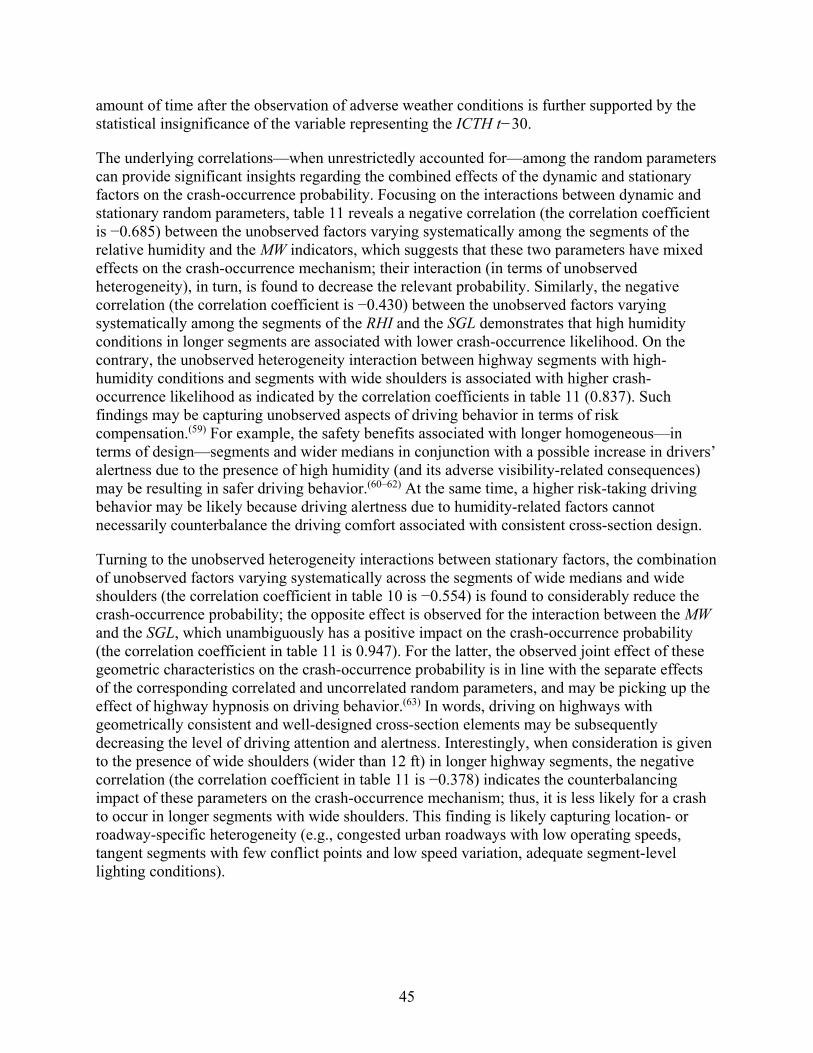
amount of time after the observation of adverse weather conditions is further supported by the statistical insignificance of the variable representing the ICTH t−30.

The underlying correlations—when unrestrictedly accounted for—among the random parameters can provide significant insights regarding the combined effects of the dynamic and stationary factors on the crash-occurrence probability. Focusing on the interactions between dynamic and stationary random parameters, table 11 reveals a negative correlation (the correlation coefficient is −0.685) between the unobserved factors varying systematically among the segments of the relative humidity and the MW indicators, which suggests that these two parameters have mixed effects on the crash-occurrence mechanism; their interaction (in terms of unobserved heterogeneity), in turn, is found to decrease the relevant probability. Similarly, the negative correlation (the correlation coefficient is −0.430) between the unobserved factors varying systematically among the segments of the RHI and the SGL demonstrates that high humidity conditions in longer segments are associated with lower crash-occurrence likelihood. On the contrary, the unobserved heterogeneity interaction between highway segments with high-humidity conditions and segments with wide shoulders is associated with higher crash-occurrence likelihood as indicated by the correlation coefficients in table 11 (0.837). Such findings may be capturing unobserved aspects of driving behavior in terms of risk compensation.(59) For example, the safety benefits associated with longer homogeneous—in terms of design—segments and wider medians in conjunction with a possible increase in drivers’ alertness due to the presence of high humidity (and its adverse visibility-related consequences) may be resulting in safer driving behavior.(60–62) At the same time, a higher risk-taking driving behavior may be likely because driving alertness due to humidity-related factors cannot necessarily counterbalance the driving comfort associated with consistent cross-section design.

Turning to the unobserved heterogeneity interactions between stationary factors, the combination of unobserved factors varying systematically across the segments of wide medians and wide shoulders (the correlation coefficient in table 10 is −0.554) is found to considerably reduce the crash-occurrence probability; the opposite effect is observed for the interaction between the MW and the SGL, which unambiguously has a positive impact on the crash-occurrence probability (the correlation coefficient in table 11 is 0.947). For the latter, the observed joint effect of these geometric characteristics on the crash-occurrence probability is in line with the separate effects of the corresponding correlated and uncorrelated random parameters, and may be picking up the effect of highway hypnosis on driving behavior.(63) In words, driving on highways with geometrically consistent and well-designed cross-section elements may be subsequently decreasing the level of driving attention and alertness. Interestingly, when consideration is given to the presence of wide shoulders (wider than 12 ft) in longer highway segments, the negative correlation (the correlation coefficient in table 11 is −0.378) indicates the counterbalancing impact of these parameters on the crash-occurrence mechanism; thus, it is less likely for a crash to occur in longer segments with wide shoulders. This finding is likely capturing location- or roadway-specific heterogeneity (e.g., congested urban roadways with low operating speeds, tangent segments with few conflict points and low speed variation, adequate segment-level lighting conditions).

45

Crash Injury-Severity Analysis Table 16 presents descriptive statistics of key variables (those that were found to be statistically significant determinants of the crash injury-severity outcomes). The estimation of the HOPIT model was based on the same dataset that was used for the crash-occurrence analysis. On the basis that the injury-severity analysis primarily leverages crash-specific data, the portion of the dataset relating to noncrash observations was not considered for this part of the analysis. Specifically, the dataset portion with only crash observations consists of 6,127 single-vehicle, police-reported crashes, from 2011 to 2013, from urban and rural highways in the State of Washington. The dataset includes information about roadway characteristics (roadway geometrics, functional class, cross-section features, and number of lanes) traffic characteristics (AADT, traffic composition, traffic-control systems, and posted speed limit) and crash-specific characteristics (injury-severity outcome; location and date of the crash; and vehicle-, driver-, and collision-specific characteristics). In addition, all the available dynamic data elements (i.e., weather information and pavement-condition information) are also included in the dataset for the injury-severity analysis.

The injury-severity outcomes were observed in four injury-severity levels: no injury (including property damage only and possible injury), injury, serious injury, and fatality. Note that the injury-severity outcome of each observation is specified as the most severe injury observed in the crash. Given the presence of many missing values in the dataset, primarily for the dynamic data elements, a portion of the dataset was used for model estimation in order to simultaneously investigate the impact of the stationary and dynamic characteristics on the injury-severity outcomes. Specifically, the final dataset consists of 2,179 single vehicle–crash observations with a full set of stationary and dynamic information. Out of these 2,179 crashes, 1,579 resulted in no injury, 555 in injury, 34 in serious injury, and 10 in fatality. With regard to the independent variables, multiple forms of the dynamic characteristics (including differential values or deviations between different time intervals) were considered in the injury-severity analysis.

46

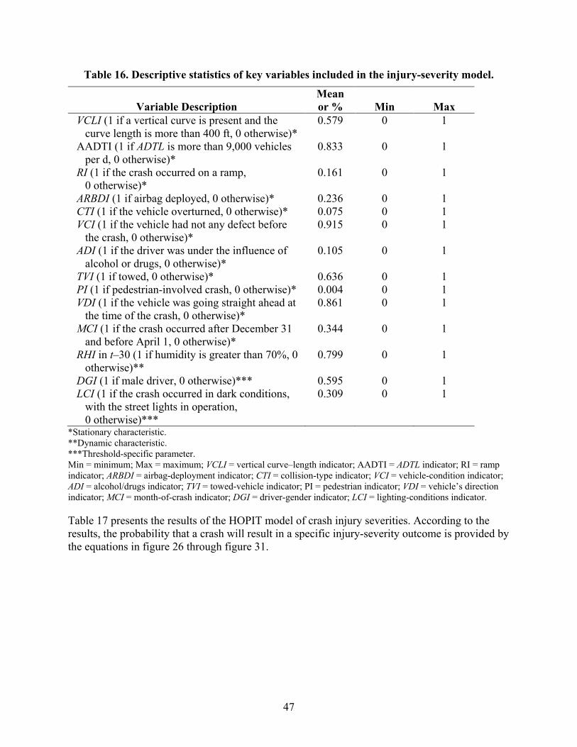
Table 16. Descriptive statistics of key variables included in the injury-severity model.

Mean Variable Description or % Min Max

VCLI (1 if a vertical curve is present and the 0.579 0 1 curve length is more than 400 ft, 0 otherwise)*

AADTI (1 if ADTL is more than 9,000 vehicles 0.833 0 1 per d, 0 otherwise)*

RI (1 if the crash occurred on a ramp, 0.161 0 1 0 otherwise)*

ARBDI (1 if airbag deployed, 0 otherwise)* 0.236 0 1 CTI (1 if the vehicle overturned, 0 otherwise)* 0.075 0 1 VCI (1 if the vehicle had not any defect before 0.915 0 1

the crash, 0 otherwise)* ADI (1 if the driver was under the influence of 0.105 0 1

alcohol or drugs, 0 otherwise)* TVI (1 if towed, 0 otherwise)* 0.636 0 1 PI (1 if pedestrian-involved crash, 0 otherwise)* 0.004 0 1 VDI (1 if the vehicle was going straight ahead at 0.861 0 1

the time of the crash, 0 otherwise)* MCI (1 if the crash occurred after December 31 0.344 0 1

and before April 1, 0 otherwise)* RHI in t–30 (1 if humidity is greater than 70%, 0 0.799 0 1

otherwise)** DGI (1 if male driver, 0 otherwise)*** 0.595 0 1 LCI (1 if the crash occurred in dark conditions, 0.309 0 1

with the street lights in operation, 0 otherwise)***

*Stationary characteristic. **Dynamic characteristic. ***Threshold-specific parameter. Min = minimum; Max = maximum; VCLI = vertical curve–length indicator; AADTI = ADTL indicator; RI = ramp indicator; ARBDI = airbag-deployment indicator; CTI = collision-type indicator; VCI = vehicle-condition indicator; ADI = alcohol/drugs indicator; TVI = towed-vehicle indicator; PI = pedestrian indicator; VDI = vehicle’s direction indicator; MCI = month-of-crash indicator; DGI = driver-gender indicator; LCI = lighting-conditions indicator.

Table 17 presents the results of the HOPIT model of crash injury severities. According to the results, the probability that a crash will result in a specific injury-severity outcome is provided by the equations in figure 26 through figure 31.

47

P (y = 1) = <P(- 0.134VCLI + 0.206AADTI + 0.463RI - 0.708ARBDI - 0 .75CTI +

0.319VCI - 0.578ADI - 0 .197TVI - 2.93PI + 0.403 VDJ + 0.137 MCI + 0.297 RH])

Table 17. Model-estimation results for the HOPIT model.

Variable Description Coefficient t-stat P-value VCLI (1 if a vertical curve is present and the curve 0.134 2.30 0.021

length is more than 400 feet, 0 otherwise)* AADTI (1 if ADTL is more than 9,000 vehicles per d, −0.206 −2.78 0.005

0 otherwise)* RI (1 if the crash occurred on a ramp, 0 otherwise)* −0.463 −2.03 0.042 ARBDI (1 if airbag deployed, 0 otherwise)* 0.708 10.66 0.000 CTI (1 if the vehicle overturned, 0 otherwise)* 0.750 5.79 0.000 VCI (1 if the vehicle had not any defect before the −0.319 −3.77 0.000

crash, 0 otherwise)* ADI (1 if the driver was under the influence of 0.578 6.48 0.000

alcohol or drugs, 0 otherwise)* TVI (1 if towed, 0 otherwise)* 0.197 3.06 0.002 PI (1 if pedestrian-involved crash, 0 otherwise)* 2.930 8.70 0.000 VDI (1 if the vehicle was going straight ahead at the −0.403 −5.51 0.000

time of the crash, 0 otherwise)* MCI (1 if the crash occurred after December 31 and −0.137 −2.23 0.026

before April 1, 0 otherwise)* RHI in t–30 (1 if humidity is greater than 70%, −0.297 −4.28 0.000

0 otherwise)** Intercept for μ1*** 0.745 10.51 0.000 Intercept for μ2*** 1.106 13.44 0.000 DGI (1 if male driver, 0 otherwise)*** −0.227 −2.85 0.004 LCI (1 if the crash occurred in dark conditions, with −0.149 −1.89 0.059

the street lights in operation, 0 otherwise)*** Number of observations 2,179 Log-likelihood at zero −1,467.228 Log-likelihood at convergence −1,308.166 McFadden pseudo-R2 0.108

*Stationary characteristic. **Dynamic characteristic. ***Threshold-specific parameter. VCLI = vertical curve–length indicator; AADTI = ADTL indicator; RI = ramp indicator; ARBDI = airbag-deployment indicator; CTI = collision-type indicator; VCI = vehicle-condition indicator; ADI = alcohol/drugs indicator; TVI = towed-vehicle indicator; PI = pedestrian indicator; VDI = vehicle’s direction indicator; MCI = month-of-crash indicator; DGI = driver-gender indicator; LCI = lighting-conditions indicator.

Figure 26. Equation. Probability of a crash resulting in no injury.

Where: P(y = 1) = probability of no injury. VCLI = vertical curve–length indicator. AADTI = ADTL indicator.

48

P(y = 2) = <P(A - 0.134VCLI +0.206AADTI + 0.463RI - 0.708ARBDI - 0.75CTI +

0.319VCI - 0.578ADI - 0.197TVl - 2.93PI +0.403VDI +0.137MCI +0.297RHl) ­

<P(- 0.134VCLI + 0.206AADTI + 0.463RI - 0.708ARBDI - 0.75CTI +

0.319VCI - 0.578ADI - 0.197TVl - 2.93PI +0.403VDI +0.137MCI +0.297RHI)

P(y = 3) = <P(/li, - 0.134VCLI +0.206AADTI +0.463RI - 0.708ARBDI- 0.75CTI + 0.319VCI - 0.578ADI - 0.197Tv7 - 2.93PI +0.403VDI + 0.137MCI +0.29iRH[) ­

<P(J4 - 0.134VCLI + 0.206AADTI +0.463RI - 0.708ARBDI - 0.75CTI + 0.319VCI - 0.578ADI - 0.197Tv7 - 2.93PI +0.403VDI + 0.137MCI +0.29iRH[)

P (y = 4) = 1- <P(;,2 - 0.1 34VCU +0 .206AADTI +0.463RI - 0.708ARBDI - 0.75CTI +

0.319VCI - 0.578ADI - 0 .197TVI - 2 .93PI + 0.403VDI + 0.137MC/ +0.297RH/)

;11 = 0.745 - 0.227DGI - 0.149LCI

RI = ramp indicator. ARBDI= airbag-deployment indicator. CTI = collision-type indicator. VCI = vehicle-condition indicator. ADI = alcohol/drugs indicator. TVI = towed-vehicle indicator. PI = pedestrian indicator. VDI = vehicle’s direction indicator. MCI = month-of-crash indicator.

Figure 27. Equation. Probability of a crash resulting in an injury.

Where: P(y = 2) = probability of injury. μ1 = upper threshold for the injury outcome.

Figure 28. Equation. Probability of a crash resulting in a serious injury.

Where: P(y = 3) = probability of serious injury. μ2 = upper threshold for the serious injury outcome.

Figure 29. Equation. Probability of a crash resulting in a fatal injury.

Where P(y = 4) is probability of fatal injury.

Figure 30. Equation. Parametric function of the threshold between the no-injury and injury outcomes.

Where: DGI = driver-gender indicator. LCI = lighting-conditions indicator.

49

p 2 = 1.106 - 0.227DGI - 0.149LCI

Figure 31. Equation. Parametric function of the threshold between the injury and serious-injury outcomes.

To better interpret the results and to identify the magnitude of the effect of each explanatory variable across the various injury-severity outcomes, table 18 presents the marginal effects of the explanatory parameters for the HOPIT model.

Table 18. Marginal effects of the explanatory variables for the HOPIT model.

Serious Fatal Variable Description No Injury Injury Injury Injury

VCLI (1 if a vertical curve is present and the curve length is more than 400 ft, 0 otherwise)*

AADTI (1 if ADTL is more than 9,000 vehicles per d, 0 otherwise)*

RI (1 if the crash occurred on a ramp, 0 otherwise)*

ARBDI (1 if airbag deployed, 0 otherwise)* CTI (1 if the vehicle overturned, 0 otherwise)* VCI (1 if the vehicle had not any defect before

the crash, 0 otherwise)* ADI (1 if the driver was under the influence of

alcohol or drugs, 0 otherwise)* TVI (1 if towed, 0 otherwise)* PI (1 if pedestrian-involved crash, 0

otherwise)* VDI (1 if the vehicle was going straight ahead

at the time of the crash, 0 otherwise)* MCI (1 if the crash occurred after

December 31 and before April 1, 0 otherwise)*

RHI in t–30 (1 if humidity is greater than 70%, 0 otherwise)**

−0.044

0.071

0.130

−0.254 −0.282

0.113

−0.212

−0.064 −0.727

0.143

0.045

0.103

0.040 0.003 0.001

−0.065 −0.005 −0.001

−0.123 −0.006 −0.001

0.226 0.024 0.004 0.242 0.033 0.007

−0.102 −0.009 −0.001

0.187 0.021 0.004

0.059 0.004 0.001 0.031 0.288 0.408

−0.129 −0.012 −0.002

−0.042 −0.003 0.000

−0.094 −0.008 −0.001

*Stationary characteristic. **Dynamic characteristic.

Turning to the estimation results of the HOPIT model, table 17 shows that 11 stationary characteristics and 1 dynamic characteristic produce statistically significant parameters that affect the injury-severity outcome probabilities, and two statistically significant parameters are found to determine the thresholds. A positive sign of a parameter in the ordered probit models indicates that the probability of the most severe outcome (i.e., fatality) increases, while the probability of the least severe outcome (i.e., no injury) decreases.

Focusing on the factors with effects that do not vary over time (i.e., stationary), several roadway-, traffic-, vehicle-, driver-, and collision-specific characteristics are found to be

50

statistically significant determinants of crash injury-severity outcomes. As far as the roadway characteristics are concerned, VCLI is found to decrease the probability of a no-injury outcome (by −0.044, as shown in table 18) and increase the probability of severe-injury outcomes (by 0.040, 0.003, and 0.001, for injury, serious injury, and fatality, respectively, as shown in table 18). On the contrary, crashes that occur on a ramp are more likely to result in no injury and less likely to result in injury outcomes of higher severity. With regard to the traffic characteristics, the variable reflecting high AADT (more than 9,000 vehicles per d) is found to increase the probability for no injury (by 0.071) and, subsequently, to decrease the probability for injury, serious injury, and fatal injury (by −0.065, −0.005, and −0.001, respectively). All these findings are in line with previous injury-severity studies.(50,54)

Turning to driver-specific characteristics, alcohol- or drug-impaired drivers are found to be associated with more severe-injury outcomes since the relevant variable (ADI) increases the probability of injury, serious injury, and fatal injury (by 0.187, 0.021, and 0.004, respectively) and decreases the probability of no injury (by −0.212). A similar effect is also observed for PI; it increases the probability of more severe outcomes (by 0.031, 0.288 and 0.408, respectively) and significantly decreases the probability of no injury (by −0.727); note that PI has the greatest (in magnitude) effect on the no-injury probability.

In regard to the vehicle-specific characteristics, table 18 shows that vehicles with good precrash condition are associated with crashes of lower injury severity. In contrast, the variable reflecting the presence of towed vehicle after the crash is found to increase the probability of more severe-injury outcomes (by 0.059, 0.004, and 0.001, for injury, serious injury, and fatality, respectively) and to decrease the probability of no injury (by −0.064). When consideration is given to the crash characteristics, the variables reflecting airbag deployment and overturned vehicles are found to result in more severe injury outcomes and may capture underlying collision-specific conditions; the opposite effect is observed for the VDI (reflecting vehicles going straight at the time of the crash), which increases the probability of no-injury outcome (by 0.143) and, in turn, decreases the probability of injury, serious injury, and fatal injury (by −0.129, −0.012, and −0.002, respectively). Furthermore, table 18 shows that crashes that occur in a winter month (January through March) are more likely to result in lower-severity outcome; such a finding is intuitive since the crash data were collected in the State of Washington, where drivers regularly experience inclement weather conditions.(50)

Focusing on the time-variant characteristics, high relative humidity (greater than 70 percent) in t–30 (which precedes the moment of the crash occurrence by 30 min) is found to increase the probability of no-injury outcome (by 0.103) and, subsequently, decrease the probability of the injury, serious injury, and fatal injury (by −0.094, −0.008, and −0.001, respectively). This finding may capture the effect of the driver’s precrash alertness due to environmental conditions associated with the presence of high humidity (reduced visibility, fog, etc.).

Turning to the threshold-specific parameters, DGI and LCI (specifically, dark conditions with the roadway-lighting infrastructure in operation) are both found to reduce the threshold values and, subsequently, to increase the likelihood for more severe crashes.

51

Model Evaluation To assess the forecasting accuracy of the random-parameters models, observed and model-predicted crash-occurrence probabilities are computed and compared. In the case of the random parameters, a separate coefficient (β) for each observation can be computed.(46) However, the computation of observation-specific coefficients can be computationally cumbersome, and most statistical software applications typically report a single coefficient for each random parameter (estimated as the average of the individual β over the observations). The mean-β predictor is useful for forecasting from sample crash-occurrence likelihoods. Even though these mean-β predictors reflect consistent and efficient parameter estimates (the random-parameters modeling scheme, by definition, addresses unobserved heterogeneity), it has been shown that their use in crash prediction is likely to yield inferior forecasts compared to the individual-β predictors.(64)

For the purposes of the TRIP project, both approaches are presented, that is, mean and individual β are used for the computation of crash-occurrence probabilities.

The forecasting accuracy of the random-parameters model estimated in phase 1 was evaluated using the mean parameter values (i.e., mean β) and individual parameter values (i.e., individual β). Table 19 and table 20 present the forecasting accuracy results of the random-parameters model using the mean parameter and individual parameter values. Under the mean-β approach, the random-parameters model correctly predicts 78 of the 138 segments without crashes (0 values), and 1,023 out of 1,047 segments with crashes (non-0 values). Under the individual-β approach, the random-parameters model correctly predicts 131 of total 138 segments without crashes and 1,045 out of 1,047 segments with crashes. Note that the sample dataset consists of 1,185 observations, which correspond to 456 roadway segments with one or more crash occurrences and 138 roadway segments with no crash occurrences. The prediction outcome is derived by the computed probability of each observation according to the following criteria:

• Prediction outcome equals 1 (a crash is likely to occur in the roadway segment) if the computed probability is equal or greater than 0.5.

• Prediction outcome equals 0 (a crash is not likely to occur in the roadway segment) if the computed probability is less than 0.5.

Table 19. Observed versus predicted crash and no-crash segments for the random-parameters model estimated in phase 1 using the mean-β approach.

Observed No. of Occurrence Segments Predicted as No Crash Predicted as Crash

No crash 138 (11.65%) 70 68 Crash 1,047 (88.35%) 24 1,023 Sum 1,185 (100%) 94 (7.93%) 1,091 (92.07%)

No. = number.

In terms of correctly and incorrectly predicted crash and no-crash segments, the results of the mean-β approach are summarized in the following list:

52

• Segments with no crashes correctly predicted as segments with no crashes: 70 out of 138 (50.7 percent).

• Segments with crashes correctly predicted as segments with crashes: 1,023 out of 1,047 (97.7 percent).

• Segments with no crashes incorrectly predicted as segments with crashes: 68 out of 138 (49.3 percent).

• Segments with crashes incorrectly predicted as segments with no crashes: 24 out of 1,047 (2.3 percent).

Table 20. Observed versus predicted crash and no-crash segments for the random-parameters model estimated in phase 1 using the individual-β approach.

Observed No. of Occurrence Segments Predicted as No Crash Predicted as Crash

No crash 138 (11.65%) 131 7 Crash 1,047 (88.35%) 1 1,046 Sum 1,185 (100%) 132 (11.14%) 1,053 (88.86%)

No. = number.

In terms of correctly and incorrectly predicted crash and no-crash segments, the results of the individual-β approach are summarized in the following list:

• Segments with no crashes correctly predicted as segments with no crashes: 131 out of 138 (95.0 percent).

• Segments with crashes correctly predicted as segments with crashes: 1,045 out of 1,047 (99.8 percent).

• Segments with no crashes incorrectly predicted as segments with crashes: 7 out of 138 (5.1 percent).

• Segments with crashes incorrectly predicted as segments with no crashes: 1 out of 1047 (0.1 percent).

As far as the phase-2 crash-occurrence models are concerned, table 21 and table 22 provide an overview and comparison of the observed and predicted probabilities for the uncorrelated-random-parameters and correlated-grouped-random-parameters models, respectively.

53

Table 21. Observed and predicted crash and no-crash segments for the uncorrelated-random-parameters model.

Observed Crash and No-Crash Occurrence Segments Individual-β Approach Mean-β Approach

Predicted Type of Predicted as Predicted as No Predicted

Occurrence No. of Segments No Crash as Crash Crash as Crash No crash 138 (11.65%) 132 6 71 67

Crash 1,047 (88.35%) 1 1,046 21 1,026 Sum 1,185 (100%) 133 1,052 92 1,093

- - 11.22% 88.78% 7.76% 92.24% -Not applicable. No. = number.

In terms of correctly predicted crash and no-crash segments, the results of the uncorrelated-random-parameters model are summarized in the following list:

• Segments with no crashes correctly predicted as segments with no crashes (individual-β approach): 132 out of 138 (95.7 percent).

• Segments with no crashes correctly predicted as segments with no crashes (mean-β approach): 71 out of 138 (51.5 percent).

• Segments with crashes correctly predicted as segments with crashes (individual-β approach): 1,046 out of 1,047 (99.9 percent).

• Segments with crashes correctly predicted as segments with crashes (mean-β approach): 1,026 out of 1,047 (97.9 percent).

In terms of incorrectly predicted crash and no-crash segments, the results of the uncorrelated-random-parameters model are summarized in the following list:

• Segments with crashes incorrectly predicted as segments with no crashes (individual-β approach): 1 out of 1,047 (0.1 percent).

• Segments with crashes incorrectly predicted as segments with no crashes (mean-β approach): 21 out of 1,047 (2.1 percent).

• Segments with no crashes incorrectly predicted as segments with crashes (individual-β approach): 6 out of 138 (4.3 percent).

• Segments with no crashes incorrectly predicted as segments with crashes (mean-β approach): 67 out of 138 (48.5 percent).

54

Table 22. Observed and predicted crash and no-crash segments for the correlated-grouped-random-parameters model.

Observed Crash and no-Crash Occurrence Segments Individual-β Approach Mean-β Approach

Predicted Predicted Type of as No Predicted as No Predicted

Occurrence No. of Segments Crash as Crash Crash as Crash No crash 138 (11.65%) 86 52 76 62

Crash 1,047 (88.35%) 5 1,042 19 1,028 Sum 1,185(100%) 91 1,094 95 1,090

- - 7.68% 92.32% 8.02% 91.98% -Not applicable. No. = number.

In terms of correctly predicted crash and no-crash segments, the results of the correlated-random-parameters model are summarized in the following list:

• Segments with no crashes correctly predicted as segments with no crashes (individual-β approach): 86 out of 138 (62.3 percent).

• Segments with no crashes correctly predicted as segments with no crashes (mean-β approach): 76 out of 138 (55.1 percent).

• Segments with crashes correctly predicted as segments with crashes (individual-β approach): 1,042 out of 1,047 (99.5 percent).

• Segments with crashes correctly predicted as segments with crashes (mean-β approach): 1,028 out of 1,047 (98.2 percent).

In terms of incorrectly predicted crash and no-crash segments, the results of the correlated-random-parameters model are summarized in the following list:

• Segments with crashes incorrectly predicted as segments with no crashes (individual-β approach): 5 out of 1,047 (0.5 percent).

• Segments with crashes incorrectly predicted as segments with no crashes (mean-β approach): 19 out of 1,047 (1.8 percent).

• Segments with no crashes incorrectly predicted as segments with crashes (individual-β approach): 52 out of 138 (37.7 percent).

• Segments with no crashes incorrectly predicted as segments with crashes (mean-β approach): 62 out of 138 (44.9 percent).

Table 21 and table 22 show that, under the individual-β approach, the uncorrelated-random-parameters model correctly predicts 132 out of 138 (95.7 percent) segments with no crashes and 1,046 out of 1,047 (nearly 100 percent) segments with crashes, whereas the correlated-grouped-

55

random-parameters approach correctly predicts 86 out of 138 (60.9 percent) segments with no crashes and 1,042 out of 1,047 (99.5 percent) segments with crashes. Under the mean-β approach, the uncorrelated-random-parameters model correctly predicts 71 out of 138 (51.5 percent) segments with no crashes, and 1,026 out of 1,047 (97.9 percent) segments with crashes; while the correlated-grouped-random-parameters model correctly predicts 76 out of 138 (55.1 percent) segments with no crashes, and 1,028 out of 1,047 (98.2 percent) segments with crashes.

At the same time, under the individual-β approach, the uncorrelated-random-parameters model yields fewer incorrect predictions (4.3 percent of segments with no crashes and 0.1 percent of segments with crashes are incorrectly predicted) compared to the correlated-grouped-random-parameters model (37.7 percent of segments with no crashes, and 0.5 percent of segments with crashes are incorrectly predicted). In contrast, under the mean-β approach, the uncorrelated-random-parameters model yields more incorrect predictions (48.5 percent of segments with no crashes, and 2.1 percent of segments with crashes are incorrectly predicted), as compared to the correlated-random-parameters model (44.9 percent of segments with no crashes, and 1.8 percent of segments with crashes are incorrectly predicted). It is important to note that the crash-occurrence probabilities of the fixed-parameters model were significantly inferior to the counterparts of the random-parameters model.

Overall, in terms of forecasting accuracy, the uncorrelated-random-parameters model outperforms its correlated counterpart, under the individual-β approach; the opposite is inferred when consideration is given to the mean-β approach, under which the correlated-grouped-random-parameters model outperforms the uncorrelated-random-parameters model. In regard to the performance of the two prediction approaches, even though the individual-β approach outperforms the mean-β approach, both approaches provide rather accurate forecasts. Factoring in the fact that the mean-β approach may be more useful in terms of out-of-sample predictability, both approaches have merits and limitations. In such manner, the correlated-grouped-random-parameters model may yield more accurate forecasts in cases of out-of-sample implementation, while it accounts for the correlation among the random parameters.

Crash-Occurrence Risk Assessment The computed probabilities are also used for the assessment of the crash-occurrence risk for each roadway segment in the sample. More specifically, for the risk-level assessment, a three-level scale was developed, which indicates three hierarchical crash-occurrence risk levels: low, moderate, and high. Each roadway segment is assigned to a risk level on the basis of the calculated probabilities. For roadway segments with more than one crash observation, the average value of the computed probabilities is used.

The comparison of the calculated probabilities with predetermined probability thresholds constitutes the fundamental criterion for the assignment of the segments to specific risk levels. For this purpose, the distribution of the resulting probabilities was investigated, and the probability thresholds were determined, as follows:

56

. TIIIPM.nM,plM..,.,• X +

C a_,_. * Q c:, ... . . = • Q TT•n•port.Uon R•n.rch lnfonnatlcs Pi.tfom1

• Roadway segments with probability less than or equal to 0.1 are considered low crash-occurrence risk.

• Roadway segments with probability between 0.1 and 0.9 are considered moderate crash-occurrence risk.

• Roadway segments with probability 0.9 or greater are considered high crash-occurrence risk.

Using the results of the random-parameters model estimated in phase 1, the risk-level assessment demonstrated that 453 out of 594 roadway segments are likely to have high crash-occurrence risk, 76 segments are likely to have moderate crash-occurrence risk, and 65 segments are likely to have low crash-occurrence risk.

On the basis of the results of the correlated-grouped-random-parameters model, which by definition addresses more complex aspects of unobserved heterogeneity and results in superior statistical fit and forecasting accuracy, the risk-level assessment demonstrates that 480 out of 594 roadway segments are likely to have high crash-occurrence risk, 45 segments are likely to have moderate crash-occurrence risk, and 69 segments are likely to have low crash-occurrence risk. An illustration of crash risk is provided in figure 32.

© 2017 CUBRC; Basemap © 2017 MapQuest.

Figure 32. Screenshot. Dynamically assigned crash risk.(22)

57

CHAPTER 6. PLATFORM SETUP AND USE

This chapter provides the documentation relevant to the installation and deployment of the key components of the platform as well as how to run the analytics. FHWA is exploring options to host the commented prototype software code and setup files in an open-source repository.

GENERAL CLUSTER SETUP

The first step in deploying TRIP involves the provisioning of a Hadoop™ Cluster to hold the analytics platform.(2) There is a wealth of information available on how to choose hardware for a Hadoop™ deployment, so it will not be discussed here. Articles from Hortonworks® and Cloudera detail the hardware requirements for their installations.(65,66) The next step is to provision the hardware with HDP.(12) The version used in TRIP is 2.5.2. Detailed installation information is provided on the Hortonworks® website.(67) Following the installation of HDP, the Anaconda Python distribution version 2.7 should be installed.(12,36,68)

WEB-SERVER SETUP

The Web-server setup requires the use of Tomcat™ 8 from Apache’s website.(25) Unzip the distribution and run bin/startup.sh. When loaded, it is possible to navigate to <your-hostname>:8080 to see instances of Tomcat™ running. To match the settings used for TRIP, replace the files in the Tomcat™ distribution with the files in Tomcat™-settings folder from the TRIP source-code folder. An overview of these settings is shown in table 23.

Table 23. Tomcat™ configuration.(25)

Setting File Description keystore/tripkeystore2 The HTTPS/SSL keystore used by

the application tomcat/bin/setenv.sh Expands the JVM heap used by

Tomcat™ tomcat/conf/server.xml Sets up HTTPS/SSL keystore

location and password and mounts Angular 2 static application(19)

tomcat/conf/tomcat-users.xml Holds login information for the Tomcat™ management application.

tomcat/conf/web.xml Adds CORS Filter settings to Web server

HTTPS = hypertext transfer protocol secure; SSL = Secure Sockets Layer; JVM = Java virtual machine; CORS = Cross-Origin Resource Sharing.

Note that, on the server.xml file, there are two hard-coded paths for the location of the keystore and Angular 2 static application.(19) Adjust these paths as needed to the target system. Similarly, to use a non-self-signed certificate adjust the Secure Sockets Layer (SSL)/Transport Layer Security connector appropriately. After these have been set, the Web-application files can be deployed to Tomcat™.(25)

59

Navigate to https://<your-hostname>/manager and login with the username/password trip/trip. Deploy the built Web-application resources to the application by clicking the “Browse…” button at the bottom of the page, selecting the WAR (Web Application Resource), and then clicking “Deploy.” As part of TRIP code delivery, two application UIs are included. One is the original phase-1, demonstration UI under “trip-web-client.” The second UI is an enhanced UI that was developed in phase 2.

GEOSERVER SETUP

The following process outlines the installation of the GeoServer stack that is utilized in the setup of TRIP.(4) Specifically, the tools outlined in table 24 will be setup and configured.

Table 24. GeoServer suite.(4)

Tool Name Version Description/Use PostgreSQL(3) 9.5 Relational Database; backend to hold data and geometries PostGIS(18) 2.2 PostGIS; adds support for geographic objects to the PostgreSQL

object-relational database pgAdmin Ⅲ 1.22.1 Administration tool for PostgreSQL GDAL(39) 2.1.1 GDAL is for reading and writing raster and vector geospatial data GeoServer 2.9.1 Connects to and serves Geo tiles and data

To set up these utilities, follow the instructions provided by the U.S. Geoscience Information Network Commons.(69)

Setting up the Database

After the database and associated tools are installed, a new database to contain the data should be created. In pgAdmin Ⅲ, connect to the database and create a new database Name the database, and run the following commands against it:

-- Enable PostGIS (includes raster) CREATE EXTENSION postgis; -- Enable Topology CREATE EXTENSION postgis_topology; -- Enable PostGIS Advanced 3D -- and other geoprocessing algorithms -- sfcgal not available with all distributions CREATE EXTENSION postgis_sfcgal; -- fuzzy matching needed for Tiger CREATE EXTENSION fuzzystrmatch; -- rule based standardizer CREATE EXTENSION address_standardizer; -- example rule data set CREATE EXTENSION address_standardizer_data_us; -- Enable US Tiger Geocoder CREATE EXTENSION postgis_tiger_geocoder;

60

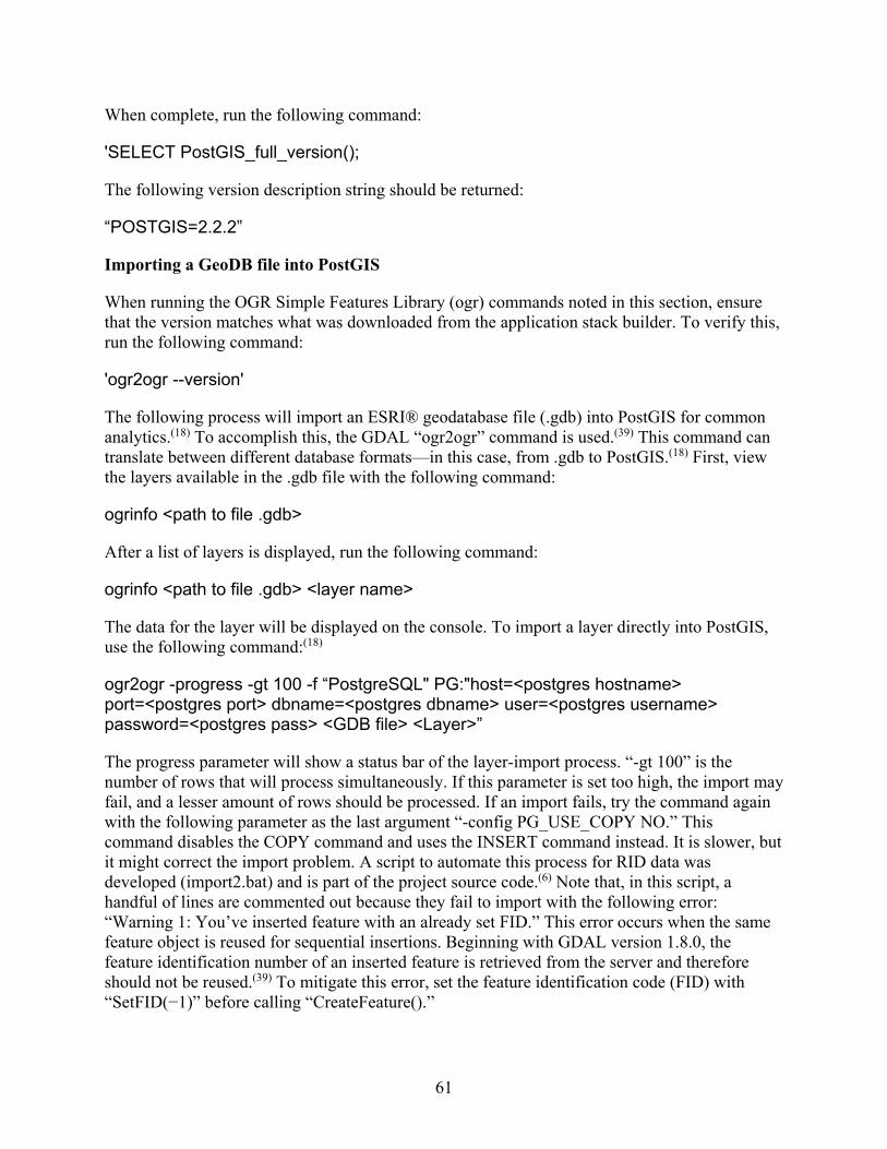
When complete, run the following command:

'SELECT PostGIS_full_version();

The following version description string should be returned:

“POSTGIS=2.2.2”

Importing a GeoDB file into PostGIS

When running the OGR Simple Features Library (ogr) commands noted in this section, ensure that the version matches what was downloaded from the application stack builder. To verify this, run the following command:

'ogr2ogr --version'

The following process will import an ESRI® geodatabase file (.gdb) into PostGIS for common analytics.(18) To accomplish this, the GDAL “ogr2ogr” command is used.(39) This command can translate between different database formats—in this case, from .gdb to PostGIS.(18) First, view the layers available in the .gdb file with the following command:

ogrinfo <path to file .gdb>

After a list of layers is displayed, run the following command:

ogrinfo <path to file .gdb> <layer name>

The data for the layer will be displayed on the console. To import a layer directly into PostGIS, use the following command:(18)

ogr2ogr -progress -gt 100 -f “PostgreSQL" PG:"host=<postgres hostname> port=<postgres port> dbname=<postgres dbname> user=<postgres username> password=<postgres pass> <GDB file> <Layer>”

The progress parameter will show a status bar of the layer-import process. “-gt 100” is the number of rows that will process simultaneously. If this parameter is set too high, the import may fail, and a lesser amount of rows should be processed. If an import fails, try the command again with the following parameter as the last argument “-config PG_USE_COPY NO.” This command disables the COPY command and uses the INSERT command instead. It is slower, but it might correct the import problem. A script to automate this process for RID data was developed (import2.bat) and is part of the project source code.(6) Note that, in this script, a handful of lines are commented out because they fail to import with the following error: “Warning 1: You’ve inserted feature with an already set FID.” This error occurs when the same feature object is reused for sequential insertions. Beginning with GDAL version 1.8.0, the feature identification number of an inserted feature is retrieved from the server and therefore should not be reused.(39) To mitigate this error, set the feature identification code (FID) with “SetFID(−1)” before calling “CreateFeature().”

61

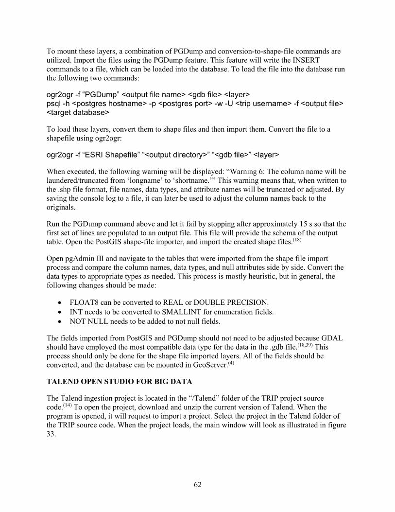
To mount these layers, a combination of PGDump and conversion-to-shape-file commands are utilized. Import the files using the PGDump feature. This feature will write the INSERT commands to a file, which can be loaded into the database. To load the file into the database run the following two commands:

ogr2ogr -f “PGDump” <output file name> <gdb file> <layer> psql -h <postgres hostname> -p <postgres port> -w -U <trip username> -f <output file> <target database>

To load these layers, convert them to shape files and then import them. Convert the file to a shapefile using ogr2ogr:

ogr2ogr -f “ESRI Shapefile” “<output directory>” “<gdb file>” <layer>

When executed, the following warning will be displayed: “Warning 6: The column name will be laundered/truncated from ‘longname’ to ‘shortname.’” This warning means that, when written to the .shp file format, file names, data types, and attribute names will be truncated or adjusted. By saving the console log to a file, it can later be used to adjust the column names back to the originals.

Run the PGDump command above and let it fail by stopping after approximately 15 s so that the first set of lines are populated to an output file. This file will provide the schema of the output table. Open the PostGIS shape-file importer, and import the created shape files.(18)

Open pgAdmin Ⅲ and navigate to the tables that were imported from the shape file import process and compare the column names, data types, and null attributes side by side. Convert the data types to appropriate types as needed. This process is mostly heuristic, but in general, the following changes should be made:

• FLOAT8 can be converted to REAL or DOUBLE PRECISION. • INT needs to be converted to SMALLINT for enumeration fields. • NOT NULL needs to be added to not null fields.

The fields imported from PostGIS and PGDump should not need to be adjusted because GDAL should have employed the most compatible data type for the data in the .gdb file.(18,39) This process should only be done for the shape file imported layers. All of the fields should be converted, and the database can be mounted in GeoServer.(4)

TALEND OPEN STUDIO FOR BIG DATA

The Talend ingestion project is located in the “/Talend” folder of the TRIP project source code.(14) To open the project, download and unzip the current version of Talend. When the program is opened, it will request to import a project. Select the project in the Talend folder of the TRIP source code. When the project loads, the main window will look as illustrated in figure 33.

62

© - C X

File Edit Wir.dow Help

l!H ill.ID ~ filk ft IJwra..d.cl '!! ~

Q Repository

in Business Models

e ~ JobDesigns

~Contexts

e ~Code

e fil'SQL Templates

e~ Metadata jl Documentation

iiiiRecyclebin

!!!!!!!I

Welcome to Talend Open Studio for Big Data

Thtspower1ul andflexit1'e tool helpsyoutakecontrol olyourdata Beloreyougetstarted, herearethet>asK:s

!!!!!!!I !!!!!!!I First, create a job using the ~

Right clK:k and select ~ Dropsource, target, andtranslormation

componentslromthe ~ toyourjob View andconf1gurethepropertiesolyourjob

components in the ~ tab

And ~nalty, use the Rl!..!!....,J__ tab toexecuteyour Job and view the results

~~ Outli l'lJ Cod 8® ~Job [f& Contexts ~ Compor.ent I ► Run job c;i Progress e@

F,~ Edt View W,l'ldl;,w Heip

11111 1.Uul tl &t tf ~ )! ~

Q RePOS>IOfY

LOCAL:TRIP .i. llusincnModds

• t • JobDnlgns

• e,cl•M

f.aC l•MHrttLo.d!obO.l

¼! CiarulMySQLl.oadJob 0.1

D cullrc_contrib C:,HSO

□ IUO_OB

D1eslir,g ~Conteiru

~ Code j1 SQL Trmpl,lln

~ Me1ac:1.,1

• Ooaiment.tlon aR«ycieti,n

=· OuU,rw, ~ ~V,t!'Wer I::) I' ~ •

, tfilelnputO..hmited_l(d1rrwteRe,;ord)

tFilelnputOelimitedJ(contriblile)

tf1lelnpul:Dehm1ted_l(1m.,ge)

tfilelnput0elimited_4(ob5lype)

tf,lelnpul:Dehm,tftl_S(obsValueM•p)

1FilelnputO..hmmed_6(o,va111z.a11on)

tFileloputDelimited_7(qchpafm}

tf,lelnpu!Dehm,ted_l (sernof)

1FilelnputOelimited_9(s«ISOfTypt)

tftlt-lnpul:0..limiter;t_lO(s,lt)

tfilelnput[)elimte<Ul{mtion)

tf1lelnpu1De11m,1ed_l2{lnptJ!f1ie)

tFilelisl_l(li.Streadingfiles)

II 139Mof 4028M ID

Q T.alf'<>d()p.-r,S1ud10 •-., XJOClaru;H,veloadJobO.l •

-~ -q­~:,o~ d,m,~,.!,., °"'~'°""'r ,,.a,~""'°"'""'°"""'°'°" '°"'a'~"'«°"''''

H.cioopS~ingP.ill Cl•n.nMet~•talociltion

3 Oi1!U$Sli1llonRodi"9l

,,.. Siring Strinsi Slri"9

I /1Mf/l.ript<1¥W a

· ·SJTRIP Pfoje,;t Oata/D•Wtl$/WA_0¥U5/Clffll5_Metal 0 "S/TRlPProfe,;t0,11,i/Oa~A_0,11\1$· 0

193Mof4047M 8

~ Palette 8@

ApalettE isr.otavailable

19 Pa1ene ~- •

f1ndcomponenL Q ~

Impala

M<mSQL ........ Neo4j

"' .. , Sqoop

8U'Sinnslnttlli9ence

© 2017 Talend.

Figure 33. Screenshot. Talend Open Studio for Big Data home screen.(14)

Figure 34 illustrates the various parts of the main Talend window.(14) The left side of the window is the repository window. This window contains two main menus, “Job Designs” and “Metadata.” The “Job Designs” menu contains all the developed jobs to import the data from the local file system to the HDFS. The “Metadata” menu contains the mapped input data schema of the different data sources and the configuration information for the Hadoop™ Cluster.(2) An example of a sample job showing how Talend transforms the data can be viewed by opening the ClarusHiveLoadJob from the “Job Designs” menu.(14,7,15)

© 2017 Talend.

Figure 34. Screenshot. Talend with a data-load job.(14)

63

This view shows the series of steps to take the information from the file data source and output it to Hadoop™.(2) The rows represent one type of file being loaded into Hadoop™, and each step is labeled to represent what it is performing. The bottom Context pane represents the global variables used throughout this job. These variables might need to be adjusted to match where the files are located on the local file system. Finally, the last variable that needs to be adjusted is network addresses of the setup Hadoop™ Cluster. Those can be found under Metadata > Hadoop Cluster. To configure the hostnames for the HDFS, right click “Hadoop Cluster,” click “Edit Hadoop Cluster,” click “next,” and adjust the Namenode Uniform Resource Identifier (URI), Resource Manager, and Resource Manager Scheduler. These configuration settings can be found in Ambari™.(13)

To adjust Hive™, spin open the Hive™ folder, right click “Edit Hive,” and adjust the settings in the pop-up menu.(15) When “Finish” is clicked, Talend will indicate that the changes made will need to be propagated to the dependent jobs.(14) Accept the propagated changes, and return to the Clarus Load Job.(7) To run the job and load the data, click the “Run” tab in the bottom window, and click the green play button. At this point, Talend will run the application and load the data into Hadoop™.(14,2) To load all of the data, click on each job, and click the play button.

JAVA, SCALA, AND WEB SOURCE CODE

The source code developed for TRIP is dependency managed using Apache Maven™ for Java code, the simple build tool (sbt) for Scala code, and node package manager (npm) for Web code.(70–72) A dependency is simply a code library on which a project depends to compile and run an application. Maven™ is a dependency specification and code management framework commonly used for java-based application development. sbt is extremely similar to Maven™ except it is designed to build Scala code. Finally, npm is used to build and manage javascript code. Commonly, Maven™ and sbt are used from the command line. When the Maven™ distribution is unzipped, make sure to include the “mvn” binary on the command line path of the local system. When sbt and npm are installed, the path should automatically update; if not, modify accordingly.

Included in the TRIP source-code folder are multiple subprojects. A listing of these subprojects, their purpose, and how to build them is displayed in table 25. Please note that these projects are only required if one wants to develop java code against the system. Prototyping functionality can be performed in Jupyter notebooks and is discussed in the following section.(9)

Table 25. TRIP subprojects.

Project Description Build Command trip-main Main code repository for TRIP mvn–DskipTests install trip-dashboarding-api Helper functions for dashboard UI sbt package trip-ui-websocket UI2 websocket code mvn–DskipTests install trip-web-app Web application code for original UI sbt package trip-web-client Original Angular Web application npm install trip-ui-2 Advanced UI npm install

64

What roadway curvature characteristics present an increased risk factor for commercial vehicles?

CUBRC

September 2nd, 2015

Last Updated: September 28th, 2015

In [ll: IImport libraries and set global options %matplotlib inline import math ~rt numpy as np import pandas as pd from scipy import stats import rnatplotlib import matplotlib . pyplot as plt from pandas . tools . plotting import table ~rom collections import defaultdict matplotlib.style . use( ' ggplot ') pd . set_option(' display . max_colurnns ' , None)

JUPYTER NOTEBOOKS

The rapid prototyping of queries and visualizations was conducted using Jupyter notebooks.(9) To validate TRIP, the sample queries detailed in chapter 4 were performed against the system. Jupyter was installed as part of the Anaconda Python distribution.(36) To start the distribution on Microsoft® Windows™, click the start button > Anaconda 2 > Launcher. When the application loads, click “Launch on IPython-notebook”. The application will load and open in a Web browser. In the browser, navigate to the IPython Notebook, code delivery in “/Jupyter Notebooks,” and open an existing .ipynb file or create a new notebook by clicking “New.” An example of an existing notebook is provided in figure 35.

© 2017 CUBRC.

Figure 35. Screenshot. Jupyter notebook analysis.(9)

All of the sample notebooks developed for TRIP and delivered with the source code can be opened, viewed, and modified. The entire notebook can be run by using the play button at the top of the screen. New cells can also be created by clicking the plus button and modifying the type of cell by clicking the adjustor labeled “Markdown.” The two major cell types are “Code” and “Markdown.” A code cell allows code in that particular cell. A markdown cell permits the entering of text in a markdown format that will be rendered into Hypertext Markup Language for viewing on a webpage. The Jupyter notebook user guide contains additional detailed information on how to develop and use Jupyter notebooks.(73,9)

ENTITY RESOLUTION

The entity-resolution tool discussed in chapter 5 was developed and tested using JetBrains IntelliJ.(74) The algorithm itself was developed within the context of a Spark™ job.(16) Utilizing Spark™ allows the algorithm to be parallelized across multiple processors or, if available, multiple nodes. The default configuration of the code uses four threads on a local machine.

65

To run the algorithm, open IntelliJ and select the option to open a project. The TRIP source-code delivery includes the IntelliJ project, so additional setup should not be needed.(74) Once the project is open, navigate to the file highlighted in left-hand project-tree view and double click to open. Once the source file is open, right click within the testData function and select the debug testData() option from the context menu. The code uses a MySQL server on the development network. The MySQL server and user login information will need to be configured by the user before the code will run as expected. The algorithm runs as a local Spark™ job, which handles the logistics of parallelization.(16) Results of the algorithm are displayed in IntelliJ’s debugger console window and finally written to a .csv file for additional analysis and importation into Hive™.(74,15)

DASHBOARDING INSTALLATION

For the dashboarding capability of the system, InfluxDB and Grafana™ technologies were utilized.(42,41) InfluxDB is a time-series database designed to store and rapidly query data with time dimensions. Grafana™ is a Web application for building metric and analytics dashboards. To install these components, first install InfluxDB followed by Grafana™. To install InfluxDB, navigate to the InfluxDB downloads page and then follow the instructions for the appropriate platform.(42) Next, install Grafana™ version 3.1.1 from the products-download section.(41) After installation, run the following influx command to create a user:

CREATE USER ‘grafana’ WITH PASSWORD ‘grafana’ WITH ALL PRIVILEGES CREATE DATABASE “trip”

Type “exit.” Navigate to grafana at <your-hostname>:3000.(41) After login, the home screen will be displayed. Click the Grafana™ logo at the upper left, and then click “Data Sources.” Using the settings in table 26, fill in the corresponding fields.

Table 26. Grafana™ setup parameters.(41)

Field Value Name InfluxDB(42)

Type InfluxDB(42)

Default Checked URL http://<server-

hostname>:8086 Database trip User Grafana™ Password Grafana™

Next, run the data-import script. To run this script, open the delivered trip-root project, and run the InfluxDBLoader class.(42) Finally, import the provided dashboards into Grafana™ by clicking the home button at the top left and then the import button at the bottom of the dropdown menu.(41) Click the “Upload .json file” button. Select a dashboard to load from the TRIP folder, and if prompted, select the InfluxDB data source created previously. Click save and open.(42)

Afterward, the dashboard can be viewed by selecting it from the top left dropdown menu.

66

DATA CHARACTERIZER/LOADER

Two applications are used to characterize and load data into PostgreSQL and PostGIS.(3,18) The data characterizer is responsible for reading data from the different data sources, automatically determining the type of data in the column and then generating a histogram that can be viewed by the user. The data loader is responsible for reading the data and transforming them so they can be queried from the UI. Both processes were written in Spark™ and are run from the command line.(16)

First, make sure the trip-main Maven™ project has been built using the mvn install command.(70)

Next, collect the two built jars defined below in the TRIP source code–alignment folder and place them in a common folder:

• data-characterization-deployer\target\data-characterization-deployer-1.0-SNAPSHOT-jar-with-dependencies.jar.

• data-alignment-deployer\target\data-alignment-deployer-1.0-SNAPSHOT-jar-with-dependencies.jar.

Download the PostgreSQL jar from Maven™ Central and place it in the same folder.(3,70) Next, connect to PostgreSQL using (pgAdmin Ⅲ, psql, etc.), and execute the PostgreSQL database setup script, postgres_setup.sql. The setup script contains all of the definitions for the table, materialized views, and stored procedures used in the TRIP application.

Next, three configuration files need to be created: hikari.properties, spark-db.properties, and spark-db-output.properties.(16) These configuration files contain the connection and database information needed to read and write records. Sample connection files are included in the delivery folder. The only modifications required are to set the user name, password, and Java Database Connectivity connection string fields for the PostgreSQL database.(3) Afterward, save and close the files. Then, run the following commands from a Linux terminal.(10) The first command will perform the data characterization; the second will load the RID data.(6)

spark-submit \ --master yarn --deploy-mode client --name “Characterize RID Data” --conf spark.driver.memory=8G --executor-cores 2 --num-executors 6 --executor-memory 8G --jars “postgresql-9.4.1212.jar” --class DataCharacterizer_162 data-characterization-deployer-1.0-

SNAPSHOT-jar-with-dependencies.jar “hikari.properties” “spark-db.properties”

spark-submit \ --master yarn \

67

--deploy-mode client \ --name “RID to JSON - New Schema” \ --conf spark.driver.memory=8G \ --executor-cores 2 \ --num-executors 6 \ --executor-memory 16G \ --jars “postgresql-9.4.1212.jar” \ --class JsonInserter data-alignment-deployer-1.0-SNAPSHOT-jar-with-dependencies.jar “spark-db.properties” “spark-db-output.properties”

After these processes have been completed, three SQL queries need to be executed to convert and build the appropriate indexes. Run the following commands:

INSERT INTO rid_all_adjusted SELECT id,

collision_report_number, datasource, city_id, county_id, time AT TIME ZONE 'PST', ST_Transform(st_geomfromtext(geom), 4326), CASE

WHEN (geom = 'POINT M EMPTY') THEN TRUE ELSE FALSE

END as geom_isempty, (json::jsonb) as json

FROM rid_all;

After running these commands, all of the data required for UI2 will have been loaded. The preceding process can be repeated for any new data in a similar format.

UI2 INSTALLATION

The second version of the TRIP UI is based on Google® Angular 2 with two minor adjustments.(19) The first adjustment is the version of Angular was updated from the beta release version in UI1 to a major release version. Second, UI2 uses angular-cli to manage the project assets and build cycle. To install angular-cli, first, ensure node.js v6.10 is installed. Next, check out the project and run the following commands. Replace the server <hostname> template with the URI of the appropriate server hostname.

npm install –g @angular/cli@1.0.0-beta.26 # navigate to ui2 project folder npm install ng build –deploy-url=http://<hostname>/ui2 --base-href=/ui2

68

A Transportation Research Informatics Platform (TRIP)

The Transportation Research Informatics Platform (TRIP) is an informatics based system designed to handle massive amounts of transportation data, provide researchers an efficient way to interact with this data, and allow for the straightforward use of analytical tools to assess the data. TRIP is an ongoing project funded under the Federal Highway Administration's Exploratory Advanced Research Program.

Transportation researchers and practitioners have access to unprecedented amounts of data but lack the tools to easily store, manipulate, and analyze this data. TRIP provides tools for researchers enabling them to conduct 'Big Data' analytics in an efficient way. The objectives of TRIP include:

TRIP architecture is flexible and is built on open source state-0f-the--art technology developed with 'Big Data' in mind. The platform consists of seven process layers 1) Infrastructure Systems; 2) Data Storage & Distribution; 3) Database & Sources; 4) Data Ingest, Transform, & Manage; 5) Data Processing, Warehousing, & Query; 6) Analytics & Visualization; and 7) Web Client & App Server. TRIP utilizes a modern, streamlined, web based user interface for remote access and query capabilities. In addition, the platform can be customized to fit exact users needs and provides linkages to many other popular analytics packages.

Although the initial objectives of TRIP were built to support transportation safety analyses the platform is capable of supporting a wide range of planning and operations activities as well . Analyses of big transportation data through an informatics approach offer opportunities to improve highway safety, reduced congestion and pollution, and more efficient incident management.

The following links provide access to the different TRIP Application endpoints:

• Phase 1 TRIP UI - Initial TRIP User Interface combining data from HSIS, RID, and Clarus. Demostrates initial, simple query building functionality, Nominatum search, Entity Resolution, and Glarus station data viewing

• Phase 2 TRIP UI - Enhanced TRIP User Interface featuring point and line data viewer and the advanced query builder. To view data for a selected point or line re-0pen another instance of the UI and click "Data Viewer" at the top of the window. Then click on a point or line

• Grafana Dashboards - Multiple different example dashboards that can be used to summarize and display data

After the ng build command has been run, a “dist/” folder is created with the Web application. This folder then can be placed in NGINX to serve the Web UI.(75)

NGINX INSTALLATION

NGINX is a multiuse Web server that can also be used as a reverse proxy, load balancer, and Hypertext Transfer Protocol cache.(75) NGINX was utilized in TRIP as a Web service and reverse proxy to serve the different UIs through one endpoint. To set up NGINX, install it via the Linux package manager using the instructions on the NGINX website.(75,10) An SSL certificate will need to be generated for NGINX.(75) To generate a self-signed certificate, use the following command:

openssl req -new -x509 -nodes -out server.crt -keyout server.key

Place the output server.crt and server.key next to the default.conf configuration file. In the default.conf file, edit each line that starts with “proxy_pass” to be the hostname of the machine on which the Tomcat™ Web server is running.(25) The process of renaming the server involves changing the hypertext transfer protocol secure address to the local Tomcat™ Web-server host and port. Next, the Web-server landing page and UI2 need to be installed. For CentOS, the files should be placed in /usr/shared/nginx.(11) UI2 should be in /usr/shared/nginx/ui2. The supplied landing page should be placed in the /usr/shared/nginx/homepage. The installation and deployment of all the TRIP components is now complete.

USING TRIP

This section provides a brief overview and tutorial on using the various components of TRIP. After installation, the TRIP home screen will look similar to figure 36.

© 2017 CUBRC.

Figure 36. Screenshot. TRIP welcome screen.

Clicking on the phase 1 TRIP UI launches the UI1 home screen as seen in figure 37.

69

A Transportation Research Informatics Platform .1. ~

0lime Range

D Beginning Date nme (UTCJ

12124/2013 12:00 AM ii D End Date nme (UTCJ

12131/2013 12:00 AM ii

□ Advanced

>_ Text Search

Search for

0 Limit results to current viewable

map area.

Q. Attribute Search

Query y

Centra l

J:RIA Lo~? Anacortes

Clallam Bay

Forks

Oui-nai-e lt Villa~

westp<>rt

" Sl<okomish

McCle.ilrv Ot Y:MPIA Abet'deen --F' Elma /

Oak• Ue '

"""""'.\ Napavine

Boi!.tfort '

Raymond

Toledo

Long B&ach Grays River i 130 km I ,._ Ska.mokawa 20 mi 1-J .. ~ _____ ...... ,.h·va11~ c::Q;XJ:G(i}' 8 Pu~l!t~ ... --.. Co~ r

Roy

Eatonville

Mossyrock

Methow

WA'SHINGTO

s Enti.lt

Wenatchee

Malaga

© 2017 CUBRC; Basemap © 2017 MapQuest.

Figure 37. Screenshot. TRIP UI1.(22)

UI1 allows access to a number of user’s tools to query and select data. In the upper left, users can construct a query based on a time range that is either continuous or sliced by hours of days or days of the week (figure 38).

70

0T1me Range

□ Beginning Date nme (UTC)

12/24/2013 12:00 AM ii D End Date nme (UTC)

12/31/2013 12:00 AM ii 0Advanced

Restrict searcn to selected days or tne weeK.

All selected (7) •

Adjust now to searcn witn lime.

® Time encapsulates entire period

0 Time is recurrent between start and end lime

>_ Text Search

Search for ...

I imit n~s.ults to r::urrP.nt viP.w;thlP. map area.

© 2017 CUBRC.

Figure 38. Screenshot. Time-range selector.

The “Text Search” box (figure 39) supports querying by name, type, or location of a place. In addition, results can be limited to an area in the current map view.

© 2017 CUBRC.

Figure 39. Screenshot. Text-search box.

The “Attribute Search” tool and Data Source Attribute Examiner (figure 40 and figure 41) can be used to select attributes from the target datasets. The data examiner permits querying of key

71

Q. Attribute Search

City/ County Selector

All selected (83) •

Add New Field

Data Source Attribute Examiner

oacaba;e

c.r;:ish_ lr:i:.

c.r;:ish_lrs

FlelCI Name

nlr.l"rol_tr.~t- ~t"1'11

s

nlr.l"rol_tr.~t_ rF.~111

Column l')'pe

0 ~r.r~1e CrJf~~nric. a l

0 ~ .r~ie Num~rir.r.l

Type Of Hit Matcnea va1ue

r.n ltmm n r1m P. ~tr.h! r.11.nhol_lP~t_

s

r.(")lt1m n 1Mm P. r~~ll r.11.nhol_lP~t_

ACld Show " --cr;-1sh_lI s c1mhitJ1Jliug_ciu:11 mstan,:e_1

0 ~ :rele C:rtl~Jlllic 31

~e111e11I in h ~IOl:Jf

am llm1t->1 1u n11~11i:e o f

A1cono - - v Number of blanK or null value;: 315156

I l istogrnm f)istrih11tion for 11ttrih11tP. 11lc.ohol_tP.st_rP.s11 lt

i ·····••11111111111111111 ••..... O O 0.1 0.2 0.3 - 0./4 0.5

terms to find target datasets and attributes that contain those terms. In addition, the examiner can also provide a preview of the distribution of the values in a histogram and allows the user to select specific values or ranges to add to the query.

© 2017 CUBRC.

Figure 40. Screenshot. Attribute-search tool.

© 2017 CUBRC.

Figure 41. Screenshot. Data source–attribute examiner.

Once the various elements of the query have been selected, they can be executed using the query button with or without the option to have the search performed in the current map view known as a Geo Search (figure 42).

72

>_ T®$:,.,,rtll

Q.JJnKf$!',;,;Jirrn

e1r,1eo,n,, S.lffl<)r

" .......... ,.,.

... lffiOIHII__,,.,_,_.,..

·-·----- ·

Query

Geo Se arch Viewable A rea

"

•

" -=• N'ID-.,

,._ .......... .-......... -....... . --

© 2017 CUBRC.

Figure 42. Screenshot. Query button with Geo Search option.

Figure 43 shows an executed query of crash data and the results. By clicking on an entity on the map, users are able to view a summary of associated attributes. There is also an option to view detailed information in a separate frame as well as the option to see information from the nearest Clarus weather station spatially and temporally (figure 44).(7)

© 2017 CUBRC; Basemap © 2017 MapQuest.

Figure 43. Screenshot. Query results and attribute information.(22)

73

0TimeRange

~ S.ginning 0 .11e Time (UTC)

11112120121200.AM

~ End 0.11e Time (UTC)

11112/2012200.AM

-· Tmel!IIC:~~lnperlod

" Tme II returrtffl l)efWleen , i,n lllCI eno tme

>_ Text search

·•l-1'- 101l-"· 1111-'1- 1011-"- 1011-" :11111-11- 11'1 :11111-11 :1111:. •1Z-t< :io•t-!!- 11,z.n 2011 !'- .,1_.,_ ·•l·" ••1-11- ·•l·" :1011-" · ••:.••- 11'1·"· ••1-u- :111•1-1• :111•1·"· 11'1 «1• ,. ttn1t 1·2:. .. ";c:~ t1n•o tt;:340 "n!c' ,1 .. ,0 11C1100 'l" '~ ,.., ,, ,a, .. , _.,~, ,202,0 •u;oo ,10..~ •1 u•o ,1oioo ·1u!~ u1><11 ••1><• 110•~• •1~•• •l9'40 . . . . . . . . . . . . . . . . . . . . . . . .

@ MapQuest

0 MapQuest Satellite

0 MapQuest Hybrid

0 MapQuest Dark

0 MapQuest Light

0 Open Street Maps

0 Stamen Toner

ONEX.RAD

Legend

Reading out of range

Crash Time

© 2017 CUBRC; Basemap © 2017 MapQuest.

Figure 44. Screenshot. Clarus weather station information.(7,22)

The layer icon in the upper right corner of the map allows users to change the basemap between several styles and has the ability to add NEXRAD radar (figure 45).

© 2017 CUBRC.

Figure 45. Screenshot. Base-layer selector.

Selecting the NEXRAD layer will import the tiles associated with the time period selected in the query (figure 46). The user then has the ability to step through images (time slider) in 5-min increments.

74

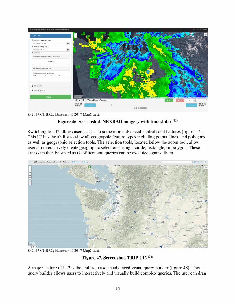
0Tmefw,ge

-, Beginning 0111• nm. (UTCI

11112120121200,t,M

" Et1C1D111• T1m.- lUTC)

11/1212012200,t,M

-, AC1v11nc•C1

-· 1" enu,psulate5 entR penoc1

IJ TimelJrec:urrenllbelweenS&Mandendtme

>_ Text Search

0.AttrouteSeafch

to12·11-12 00:00:00 -

■ Q Trans portation RHHrch lnfonnatk1 f>tatform O Broww P O y

--·~

= s ® ...... ~~-----------------~---~----

--

to12•11-12 O2:la:OO

£ H K1. 11 0

0 - e

© 2017 CUBRC; Basemap © 2017 MapQuest.

Figure 46. Screenshot. NEXRAD imagery with time slider.(22)

Switching to UI2 allows users access to some more advanced controls and features (figure 47). This UI has the ability to view all geographic feature types including points, lines, and polygons as well as geographic selection tools. The selection tools, located below the zoom tool, allow users to interactively create geographic selections using a circle, rectangle, or polygon. These areas can then be saved as Geofilters and queries can be executed against them.

© 2017 CUBRC; Basemap © 2017 MapQuest.

Figure 47. Screenshot. TRIP UI2.(22)

A major feature of UI2 is the ability to use an advanced visual query builder (figure 48). This query builder allows users to interactively and visually build complex queries. The user can drag

75

(p) , ..

= {11 SR 99: S Otarborn St

Filterbyfleld(a lcohol tet.lJHUlt) 41c.11~t. selected.

MapOfArH

"""'-Seattle Seahawt(s Query

Select a field to view browse it's contents.

Field Name Field "Type

... I 5 141 5:\5 iii 1#-:I I

@ldenliler(&) @ OGcretecategontlll(156) @NumentC.tegonu,1(23) @ l«.metitC0nlll'luout(A) @ Slanc!MllCOMmt.(3)

Ad)us1Viewablehelds

@ Hide tu WIUe$? @ I-toe Zettl vauet? D Hide lllalW WIUe$?

~ !Ill::. 2017-03-09 ~ :05:liOPM

' ii e:ten-.. .}-,-• ,.-•

Updated Right Now!

(3)3rdAYeS (A)4rdAYeS (SI 1.,oAJrport WrJ. WI

1, tt, Kevin! O

View ... --

(6)1thAveS.H

and drop components into a frame to select various data elements and attributes and then subject them to geographic or Boolean operations. As in UI1, users can also preview the values of a selected attribute in a histogram and then selectvalues to be included in the query. Once a query has been constructed, it can be saved as a graphlet for future use or modification.

© 2017 CUBRC.

Figure 48. Screenshot. UI2 advanced visual query builder.

Finally, TRIP users also have the ability to utilize and customize several prebuilt dashboards that display crash, weather, and traffic-camera information for the Seattle region (figure 49). Users can change the county, collision severity, and time periods using the dropdown menus. In addition, users can create their own dashboards or modify the existing dashboards.

© 2017 CUBRC; Basemap © 2017 MapQuest, Traffic Images © 2017 WSDOT.

Figure 49. Screenshot. Weather dashboard with traffic cameras.(22)

76

CHAPTER 7. SUMMARY

It is clear that optimizing the utility of the vast amount of data available to transportation safety analysts now and in the near future, including SHRP2 NDS data, is a challenging and complex task.(1) For this reason, it is necessary to develop tools to handle and analyze data in an efficient manner. TRIP is an end-to-end informatics-based system designed to handle massive amounts and many forms of transportation data, provide researchers an efficient way to interact with data, and provides straightforward tools to analyze data. TRIP has been designed to be highly customizable and function with both legacy and innovative data stores.

TRIP consists of several integrated process layers that provide the core functionality of the system. The first layer provides the infrastructure system for the platform utilizing the CentOS Linux operating system.(11,10) The second layer provides data storage, processing, and management solutions based on the Hadoop™ framework.(2) In order to ingest, transform, align, and store structured, semistructured, and unstructured data, tools, such as Talend and GDAL, and management tools, including Ambari™, have been employed.(14,39,13) Data-processing, -warehousing, and -query functionality are provided by Spark™ and Hive™, PostgreSQL, while PostGIS provides advanced geospatial capabilities. (See references 16, 15, 3, and 18.) TRIP was designed to provide great flexibility to analysts and researchers. As such, linkages to many popular analytics packages and visualization tools have been developed.

As part of the initial development and demonstration of TRIP, sample datasets from the Seattle, WA, region have been ingested, transformed, aligned, and stored. The first dataset was from HSIS and has information on crashes on State roads, traffic volumes, and characteristics of facilities, including curve and grade.(5) RID, from the SHRP2 NDS program, contains detailed information on roadway geometrics and attributes.(6,1) It also contains supplemental information on historical crashes, volumes, weather, traffic laws, safety campaigns, and work zones. Data from the Clarus Initiative provide complete information on atmospheric camera feeds and were also incorporated.(7) In order to demonstrate the functionality of the overall system, several user access points and interfaces were developed.

TRIP utilizes a modern, streamlined, Web-based UI for remote access and query capabilities. The UI provides basic analytics and visualization through the use of an interactive visual query builder and data characterizer and viewer. These analytics provide access to temporal, categorical, and spatial queries as well as visualization of the datasets and linkages. Temporal queries can be performed by selecting desired time frames, continuous as well as segmented by hours of interest. The categorical search tool allows analysts to select desired attributes of interest through an indexed data characterizer, thus not requiring in depth knowledge of the source metadata. The spatial-query tools allow for the interactive selection of specific locations through the use of an on-screen display. The results and attributes are made instantly available in a separate data window. In the example presented, the unified UI provides the ability to view HSIS crash information, RID roadway data along with the closest Clarus weather data (both time and space), and NEXRAD radar imagery.(5–7)

The capabilities of TRIP can be extended and customized to user’s needs by providing linkages to many popular analytics packages such as R, SAS®, MathWorks® MATLAB®, Microsoft®

77

Excel™, etc. As an example of this linkage, and to provide a demonstration of the full potential of the platform, Jupyter notebooks have been incorporated. Notebooking technology provides analysts a way to collect code and run code, provide text descriptions and visualizations, and develop and test models all in one place.(9) They also have to ability to import a rich set of libraries with previously designed algorithms or models that can be customized and executed against the full set of data ingested in the platform. Finally, as another extension, dashboarding capabilities have been provided as a rapid way to summarize and visualize streaming and historical data. Specific examples have been developed that provide summary information on crash information in graph and tabular forms along with supplemental weather and traffic camera information.

A potential limiting factor in transportation-safety research has been the reliance on relatively small, isolated datasets. For example, many safety analyses primarily depend upon historical crash databases, such as the Fatality Awareness Reporting System, the National Automotive Sampling System, and Special Crash Investigations, collected by the National Highway Traffic Safety Administration. These datasets include sparse roadway-characterization data and limited weather information. In some cases, these datasets do not contain data that accurately reflect the technology and features of the current vehicle fleet or the existing features and conditions of the highway systems. The current state of the art in transportation research is finding ways to utilize massive or novel data sources to solve these problems. Examples of this kind of data include vehicle-to-vehicle, vehicle-to-infrastructure, mobile phones, and other sensor data. While each of these data resources provide a wealth of data, their structure, size, and quality can be challenging to use. To take advantage of the vast amount of data available, it is necessary to develop tools like TRIP to handle and analyze the data in an efficient manner.

The analyses of big data through an informatics-based approach offer great promise for a new generation of advancements in transportation, including improved highway-vehicle management, reduced congestion and pollution, and most importantly, safer roadways. The value of this approach comes from its ability to establish linkages between large, disparate datasets and then use tools to identify patterns and insights in the data that were not otherwise apparent. The initial objectives of TRIP were to support transportation-safety analyses, but the platform is also capable of supporting a wide range of planning, maintenance, and operations activities. Analyses of big transportation data through an informatics approach offer opportunities to improve highway safety, reduce congestion and pollution, and ensure more efficient incident management.

This project has developed, demonstrated, and delivered an informatics-based system to handle massive amounts of transportation data to allow researchers to query features/events and utilize analytics to assess the results. This system provides transportation safety analysts new tools and access to data in order to further their understanding of transportation safety–related issues. Although further development and testing is necessary, it is the goal to make TRIP readily available to transportation research, planning, and operations agencies for use in real-world analyses.

78

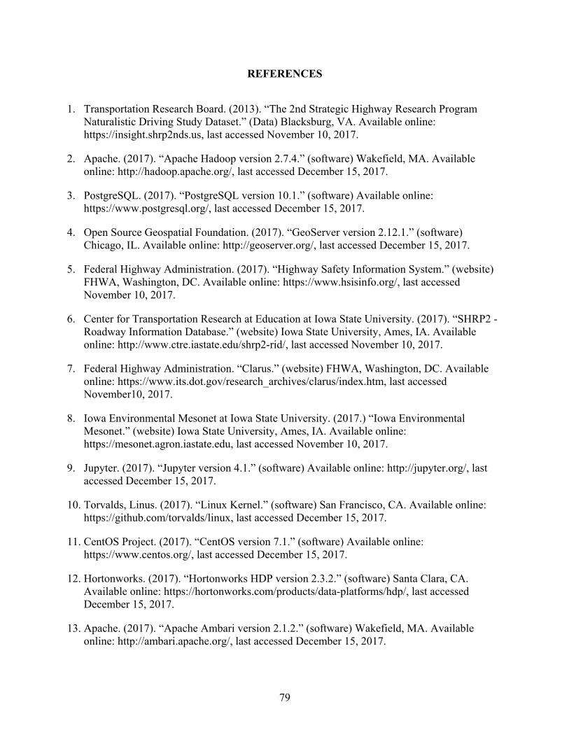
REFERENCES

1. Transportation Research Board. (2013). “The 2nd Strategic Highway Research Program Naturalistic Driving Study Dataset.” (Data) Blacksburg, VA. Available online: https://insight.shrp2nds.us, last accessed November 10, 2017.

2. Apache. (2017). “Apache Hadoop version 2.7.4.” (software) Wakefield, MA. Available online: http://hadoop.apache.org/, last accessed December 15, 2017.

3. PostgreSQL. (2017). “PostgreSQL version 10.1.” (software) Available online: https://www.postgresql.org/, last accessed December 15, 2017.

4. Open Source Geospatial Foundation. (2017). “GeoServer version 2.12.1.” (software) Chicago, IL. Available online: http://geoserver.org/, last accessed December 15, 2017.

5. Federal Highway Administration. (2017). “Highway Safety Information System.” (website) FHWA, Washington, DC. Available online: https://www.hsisinfo.org/, last accessed November 10, 2017.

6. Center for Transportation Research at Education at Iowa State University. (2017). “SHRP2 -Roadway Information Database.” (website) Iowa State University, Ames, IA. Available online: http://www.ctre.iastate.edu/shrp2-rid/, last accessed November 10, 2017.

7. Federal Highway Administration. “Clarus.” (website) FHWA, Washington, DC. Available online: https://www.its.dot.gov/research_archives/clarus/index.htm, last accessed November10, 2017.

8. Iowa Environmental Mesonet at Iowa State University. (2017.) “Iowa Environmental Mesonet.” (website) Iowa State University, Ames, IA. Available online: https://mesonet.agron.iastate.edu, last accessed November 10, 2017.

9. Jupyter. (2017). “Jupyter version 4.1.” (software) Available online: http://jupyter.org/, last accessed December 15, 2017.

10. Torvalds, Linus. (2017). “Linux Kernel.” (software) San Francisco, CA. Available online: https://github.com/torvalds/linux, last accessed December 15, 2017.

11. CentOS Project. (2017). “CentOS version 7.1.” (software) Available online: https://www.centos.org/, last accessed December 15, 2017.

12. Hortonworks. (2017). “Hortonworks HDP version 2.3.2.” (software) Santa Clara, CA. Available online: https://hortonworks.com/products/data-platforms/hdp/, last accessed December 15, 2017.

13. Apache. (2017). “Apache Ambari version 2.1.2.” (software) Wakefield, MA. Available online: http://ambari.apache.org/, last accessed December 15, 2017.

79

14. Talend. (2017). “Talend version 6.1.” (software) Redwood City, CA. Available online: https://www.talend.com/, last accessed December 15, 2017.

15. Apache. (2017). “Apache Hive version 2.3.2.” (software) Wakefield, MA. Available online: http://hive.apache.org/, last accessed December 15, 2017.

16. Apache. (2017). “Apache Spark version 2.2.1.” (software) Wakefield, MA. Available online: http://spark.apache.org/, last accessed December 15, 2017.

17. Apache. (2017). “Apache HBase version 1.4.0.” (software) Wakefield, MA. Available online: http://hbase.apache.org/, last accessed December 15, 2017.

18. PostGIS. (2017). “PostGIS version 2.4.0.” (software) Available online: https://postgis.net/, last accessed December 15, 2017.

19. Google®. (2017). “Google Angular 2 version 5.0.0.” (software) Mountain View, CA. Available online: https://angular.io/, last accessed December 15, 2017.

20. Agafonkin, Vladimir. (2017). “Leaflet version 1.2.0.” (software) Available online: http://leafletjs.com/, last accessed December 15, 2017.

21. OpenStreetMap. (2017). “OpenStreetMap.” (website) Available online: https://www.openstreetmap.org/, last accessed December 15, 2017.

22. MapQuest. (2017). “MapQuest.” (website) MapQuest, Denver, CO. Available online: https://www.mapquest.com/, last accessed December 15, 2017.

23. ESRI. (2017). “ESRI ArcGIS version 10.3.1.” (software) Redlands, CA. Available online: http://www.esri.com/arcgis/about-arcgis, last accessed December 15, 2017.

24. GeoServer. (2017). “GeoServer Documentation.” (website) Open Source Geospatial Foundation, Beaverton, OR. Available online: http://docs.geoserver.org/, last accessed November 10, 2017.

25. Apache. (2017). “Apache Tomcat version 8.0.21.” (software) Wakefield, MA. Available online: http://tomcat.apache.org/, last accessed December 15, 2017.

26. Scalatra. (2017). “Scalatra version 2.6.0.” (software) Available online: http://scalatra.org/, last accessed December 15, 2017.

27. Oracle. (2017). “Oracle Jersey version 2.26.” (software) Redwood Shores, CA. Available online: https://jersey.github.io/, last accessed December 15, 2017.

28. Async-IO.org (2017). “Atmosphere version 2.1.0.” (software) Available online: https://github.com/Atmosphere/atmosphere, last accessed December 15, 2017.

80

29. Federal Highway Administration. (2017). “Highway Safety Information System Guidebook for the Washington State Data Files.” (website) FHWA, Washington, DC. Available online: http://www.hsisinfo.org/guidebooks/washington.cfm, last accessed November 10, 2017.

30. Federal Highway Administration. (2018). “Projects and Programs.” (website) FHWA, Washington, DC. Available online: https://ops.fhwa.dot.gov/weather/mitigating_impacts/programs.htm, last accessed October 31, 2018.

31. Federal Highway Administration. (2017). “Weather Data Environment.” (website) FHWA, Washington, DC. Available online: https://74.254.188.153/auth2/metadata.jsp, last accessed November 10, 2017.

32. Scikit-learn. (2017). “Scikit-learn version 0.18.2.” (software) Available online: http://scikit-learn.org/, last accessed December 15, 2017.

33. Pandas. (2017). “Pandas version 0.21.0.” (software) Available online: https://pandas.pydata.org/, last accessed December 15, 2017.

34. Story, Rob. (2017). “Folium version 0.6.0.” (software) Available online: https://github.com/python-visualization/folium, last accessed December 15, 2017.

35. SciPy. (2017). “SciPy tool stack 1.0.0.” (software) Available online: https://www.scipy.org/, last accessed December 15, 2017.

36. Anaconda (2017). “Anaconda Distribution version 5.0.1.” (software) Austin, TX. Available online: https://www.anaconda.com/distribution, last accessed December 15, 2017.

37. Apache. (2017). “Apache Zeppelin version 0.7.3.” (software) Wakefield, MA. Available online: http://zeppelin.apache.org/, last accessed December 15, 2017.

38. American Association of State Highway and Transportation Officials. (2014). Highway Safety Manual. AASHTO, Washington, DC. Available online: http://www.highwaysafetymanual.org/Pages/hsm_parts.aspx#partb, last accessed December 15, 2017.

39. Open Source Geospatial Foundation. (2017). “Geospatial Data Abstraction Library version 2.2.3.” (software) Available online: http://www.gdal.org/, last accessed December 15, 2017.

40. pgAdmin. (2017). “pgAdmin III version 1.22.1” (software) Available online: https://www.pgadmin.org/, last accessed December 2017.

41. Coding Instinct. (2017). “Grafana version 4.6.3.” (software) Stockholm, Sweden. Available online: https://grafana.com/, last accessed December 15, 2017.

42. InfluxData Inc. (2017). “InfluxDB 1.6.4.” (software) San Francisco, CA. Available online: https://www.influxdata.com/time-series-platform/influxdb/, last accessed December 15, 2017.

81

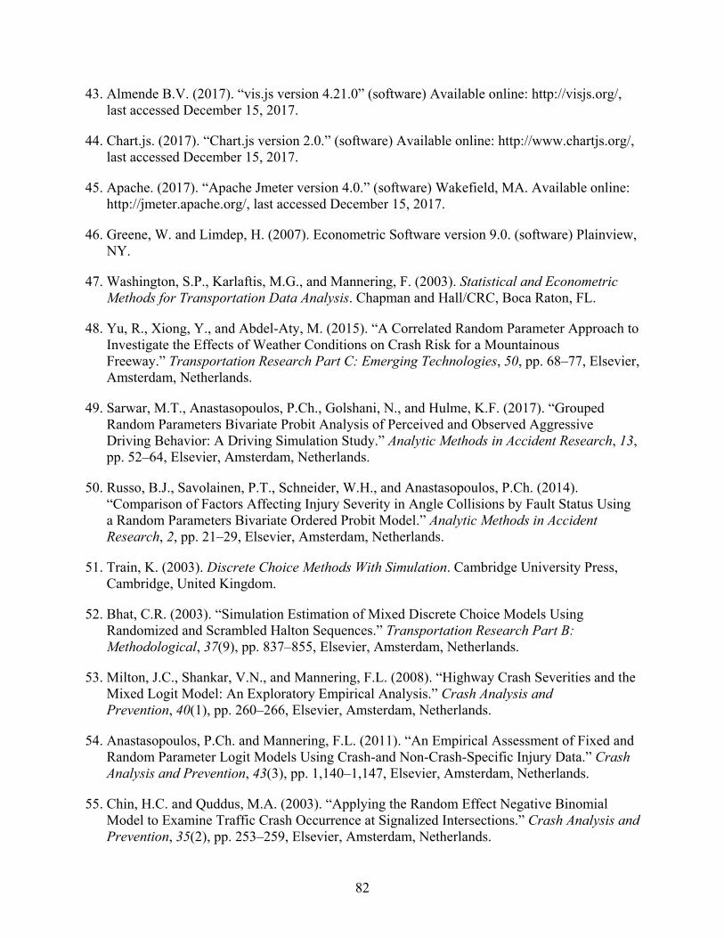
43. Almende B.V. (2017). “vis.js version 4.21.0” (software) Available online: http://visjs.org/, last accessed December 15, 2017.

44. Chart.js. (2017). “Chart.js version 2.0.” (software) Available online: http://www.chartjs.org/, last accessed December 15, 2017.

45. Apache. (2017). “Apache Jmeter version 4.0.” (software) Wakefield, MA. Available online: http://jmeter.apache.org/, last accessed December 15, 2017.

46. Greene, W. and Limdep, H. (2007). Econometric Software version 9.0. (software) Plainview, NY.

47. Washington, S.P., Karlaftis, M.G., and Mannering, F. (2003). Statistical and Econometric Methods for Transportation Data Analysis. Chapman and Hall/CRC, Boca Raton, FL.

48. Yu, R., Xiong, Y., and Abdel-Aty, M. (2015). “A Correlated Random Parameter Approach to Investigate the Effects of Weather Conditions on Crash Risk for a Mountainous Freeway.” Transportation Research Part C: Emerging Technologies, 50, pp. 68–77, Elsevier, Amsterdam, Netherlands.

49. Sarwar, M.T., Anastasopoulos, P.Ch., Golshani, N., and Hulme, K.F. (2017). “Grouped Random Parameters Bivariate Probit Analysis of Perceived and Observed Aggressive Driving Behavior: A Driving Simulation Study.” Analytic Methods in Accident Research, 13, pp. 52–64, Elsevier, Amsterdam, Netherlands.

50. Russo, B.J., Savolainen, P.T., Schneider, W.H., and Anastasopoulos, P.Ch. (2014). “Comparison of Factors Affecting Injury Severity in Angle Collisions by Fault Status Using a Random Parameters Bivariate Ordered Probit Model.” Analytic Methods in Accident Research, 2, pp. 21–29, Elsevier, Amsterdam, Netherlands.

51. Train, K. (2003). Discrete Choice Methods With Simulation. Cambridge University Press, Cambridge, United Kingdom.

52. Bhat, C.R. (2003). “Simulation Estimation of Mixed Discrete Choice Models Using Randomized and Scrambled Halton Sequences.” Transportation Research Part B: Methodological, 37(9), pp. 837–855, Elsevier, Amsterdam, Netherlands.

53. Milton, J.C., Shankar, V.N., and Mannering, F.L. (2008). “Highway Crash Severities and the Mixed Logit Model: An Exploratory Empirical Analysis.” Crash Analysis and Prevention, 40(1), pp. 260–266, Elsevier, Amsterdam, Netherlands.

54. Anastasopoulos, P.Ch. and Mannering, F.L. (2011). “An Empirical Assessment of Fixed and Random Parameter Logit Models Using Crash-and Non-Crash-Specific Injury Data.” Crash Analysis and Prevention, 43(3), pp. 1,140–1,147, Elsevier, Amsterdam, Netherlands.

55. Chin, H.C. and Quddus, M.A. (2003). “Applying the Random Effect Negative Binomial Model to Examine Traffic Crash Occurrence at Signalized Intersections.” Crash Analysis and Prevention, 35(2), pp. 253–259, Elsevier, Amsterdam, Netherlands.

82

56. Vogt, A. and Bared, J. (1998). “Crash Models for Two-Lane Rural Segments and Intersections.” Transportation Research Record, 1635, pp. 18–29, Transportation Research Board, Washington, DC.

57. Anastasopoulos, P.Ch. and Mannering, F.L. (2009). “A Note on Modeling Vehicle Crash Frequencies With Random-Parameters Count Models.” Crash Analysis and Prevention, 41(1), pp. 153–159, Elsevier, Amsterdam, Netherlands.

58. Venkataraman, N., Ulfarsson, G.F., and Shankar, V.N. (2013). “Random Parameter Models of Interstate Crash Frequencies by Severity, Number of Vehicles Involved, Collision and Location Type.” Crash Analysis and Prevention, 59, pp. 309–318, Elsevier, Amsterdam, Netherlands.

59. Mannering, F.L. and Bhat, C.R. (2014). “Analytic Methods in Crash Research: Methodological Frontier and Future Directions.” Analytic Methods in Accident Research, 1, pp. 1–22, Elsevier, Amsterdam, Netherlands.

60. Knuiman, M., Council, F., and Reinfurt, D. (1993). “The Effect of Median Width on Highway Crash Rates.” Transportation Research Record, 1401, pp. 70–80, Transportation Research Board, Washington, DC.

61. Hadi, M.A., Aruldhas, J., Chow, L.F., and Wattleworth, J.A. (1995). “Estimating Safety Effects of Cross-Section Design for Various Highway Types Using Negative Binomial Regression.” Transportation Research Record, 1500, p. 169, Transportation Research Board, Washington, DC.

62. Abdel-Aty, M.A. and Radwan, A.E. (2000). “Modeling Traffic Crash Occurrence and Involvement.” Crash Analysis and Prevention, 32(5), pp. 633–642, Elsevier, Amsterdam, Netherlands.

63. Winston, C., Maheshri, V., and Mannering, F. (2006). “An Exploration of the Offset Hypothesis Using Disaggregate Data: The Case of Airbags and Antilock Brakes.” Journal of Risk and Uncertainty, 32(2), pp. 83–99, Springer, Basingstoke, UK.

64. Anastasopoulos, P.Ch. (2016). “Random Parameters Multivariate Tobit and Zero-Inflated Count Data Models: Addressing Unobserved and Zero-State Heterogeneity in Crash Injury-Severity Rate and Frequency Analysis.” Analytic Methods in Accident Research, 11, pp. 17– 32, Elsevier, Amsterdam, Netherlands.

65. Baldeschieler, E. (2011). “Best Practices for Selecting Apache Hadoop Hardware.” (blog) Hortonworks, Santa Clara, CA. Available online: https://hortonworks.com/blog/best-practices-for-selecting-apache-hadoop-hardware/, last accessed November 10, 2017.

66. O’Dell, K. (2013). “How-to: Select the Right Hardware for Your New Hadoop Cluster.” (blog) Cloudera, Palo Alto, CA. Available online: http://blog.cloudera.com/blog/2013/08/how-to-select-the-right-hardware-for-your-new-hadoop-cluster/, last accessed November 10, 2017.

83

67. Hortonworks. (2017). “Apache Ambari Installation” (website) Santa Clara, CA. Available online: https://docs.hortonworks.com/HDPDocuments/Ambari-2.6.2.0/bk_ambari-installation/content/ch_Deploy_and_Configure_a_HDP_Cluster.html, last accessed November 10, 2017.

68. Anaconda. (2017). “Download Anaconda Distribution.” (website) Austin, TX. Available online: https://www.anaconda.com/download/, last accessed November 10, 2017.

69. U.S. Geoscience Information Network Commons. (2013). “Convert File GDB to PostGIS Database.” (website) Tucson, AZ. Available online: http://lab.usgin.org/groups/best-practices-usgin-web-service-hosting/convert-file-gdb-postgis-database, last accessed November 10, 2017.

70. Apache. (2017). “Apache Maven version 3.3” (software) Wakefield, MA. Available online: http://maven.apache.org/, last accessed December 15, 2017.

71. Lightbend. (2017). “sbt version 1.2.6.” (software) San Francisco, CA. Available online: https://www.scala-sbt.org/, last accessed December 15, 2017.

72. npm. “npm version 10.13.0.” (software) Oakland, CA. Available online: https://www.npmjs.com/get-npm, last accessed December 15, 2017.

73. Jupyter. (2017). “The Jupyter Notebook.” (website) Available online: https://jupyter-notebook.readthedocs.io/en/latest/, last accessed November 10, 2017.

74. JetBrains. (2017). “IntelliJ version 2017.2.2.” (software) Available online: https://github.com/JetBrains/intellij-community, last accessed December 15, 2017.

75. NGINX. (2017). “NGINX version 1.13.” (software) San Francisco, CA. Available online: http://hg.nginx.org/nginx/, last accessed December 15, 2017.

84

HRDS-01/01-19(WEB)E