applications of differentiation

APPLICATIONS OF DIFFERENTIATIONAPPLICATIONS OF DIFFERENTIATION

4

APPLICATIONS OF DIFFERENTIATION

So far, we have been concerned with some

particular aspects of curve sketching:

Domain, range, and symmetry (Chapter 1) Limits, continuity, and asymptotes (Chapter 2) Derivatives and tangents (Chapters 2 and 3) Extreme values, intervals of increase and decrease,

concavity, points of inflection, and l’Hospital’s Rule (This chapter)

It is now time to put all this information

together to sketch graphs that reveal

the important features of functions.


4.5Summary of

Curve Sketching

In this section, we will learn:

How to draw graphs of functions

using various guidelines.


SUMMARY OF CURVE SKETCHING

You might ask:

Why don’t we just use a graphing calculator or computer to graph a curve?

Why do we need to use calculus?

It’s true that modern technology

is capable of producing very accurate

graphs.

However, even the best graphing devices have to be used intelligently.



We saw in Section 1.4 that it is extremely

important to choose an appropriate viewing

rectangle to avoid getting a misleading graph.

See especially Examples 1, 3, 4, and 5 in that section.

The use of calculus enables us to:

Discover the most interesting aspects of graphs.

In many cases, calculate maximum and minimum points and inflection points exactly instead of approximately.



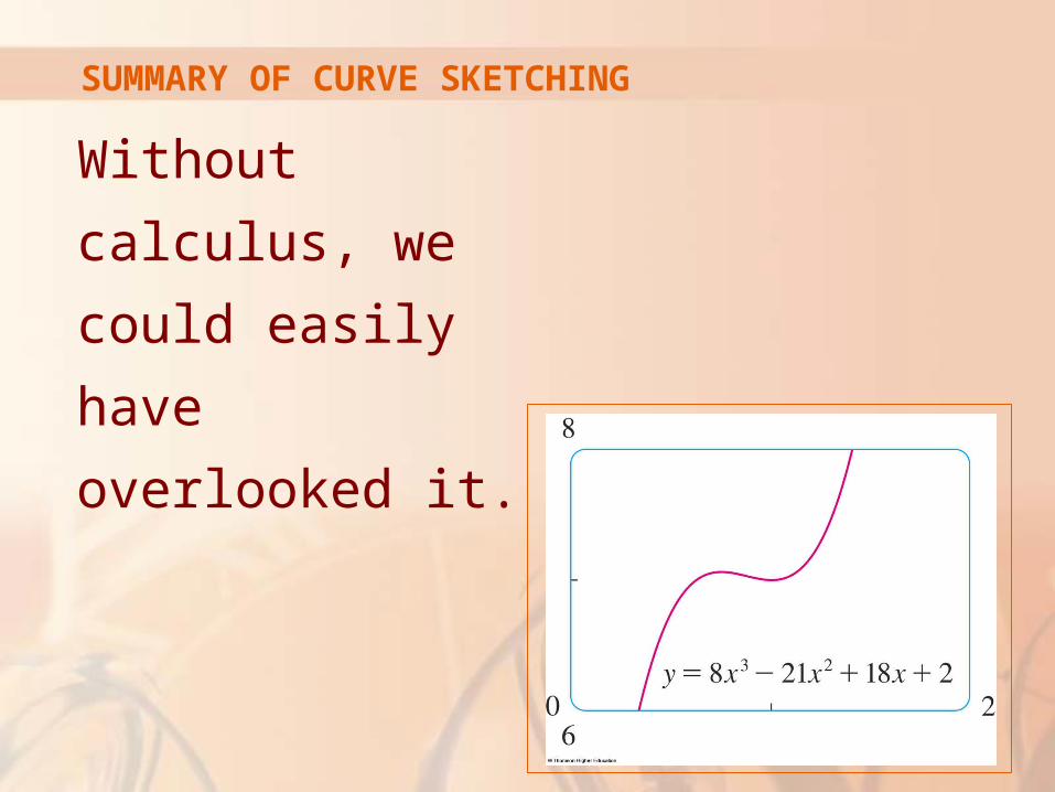
For instance, the

figure shows

the graph of:

f(x) = 8x3 - 21x2 +

18x + 2


At first glance, it

seems reasonable:

It has the same shape as cubic curves like y = x3.

It appears to have no maximum or minimum

point.


However, if you compute

the derivative,

you will see that there is

a maximum when

x = 0.75 and a minimum

when x = 1.

Indeed, if we zoom in to this portion of the graph, we see that behavior exhibited in the next figure.


Without calculus,

we could easily

have overlooked it.


In the next section, we will graph

functions by using the interaction

between calculus and graphing devices.


In this section, we draw graphs by first

considering the checklist that follows.

We don’t assume that you have a graphing device.

However, if you do have one, you should use it as a check on your work.

GUIDELINES FOR SKETCHING A CURVE

The following checklist is intended as a

guide to sketching a curve y = f(x) by hand.

Not every item is relevant to every function. For instance, a given curve might not have

an asymptote or possess symmetry. However, the guidelines provide all the information

you need to make a sketch that displays the most important aspects of the function.

A. DOMAIN

It’s often useful to start by determining

the domain D of f.

This is the set of values of x for which f(x) is defined.

B. INTERCEPTS

The y-intercept is f(0) and this tells us

where the curve intersects the y-axis.

To find the x-intercepts, we set y = 0

and solve for x.

You can omit this step if the equation is difficult to solve.

C. SYMMETRY—EVEN FUNCTION

If f(-x) = f(x) for all x in D, that is, the equation

of the curve is unchanged when x is replaced

by -x, then f is an even function and the curve

is symmetric about the y-axis.

This means that our work is cut in half.


If we know what the

curve looks like for x ≥ 0,

then we need only reflect

about the y-axis to obtain

the complete curve.


Here are some

examples:

y = x2

y = x4

y = |x| y = cos x

If f(-x) = -f(x) for all x in D, then f

is an odd function and the curve is

symmetric about the origin.

C. SYMMETRY—ODD FUNCTION


Again, we can obtain

the complete curve

if we know what it looks

like for x ≥ 0.

Rotate 180°

about the origin.


Some simple

examples of odd

functions are:

y = x y = x3

y = x5

y = sin x

If f(x + p) = f(x) for all x in D, where p

is a positive constant, then f is called

a periodic function.

The smallest such number p is called

the period.

For instance, y = sin x has period 2π and y = tan x has period π.

C. SYMMETRY—PERIODIC FUNCTION

C. SYMMETRY—PERIODIC FUNCTION

If we know what the

graph looks like in

an interval of length p,

then we can use

translation to sketch the

entire graph.

D. ASYMPTOTES—HORIZONTAL

Recall from Section 2.6 that, if either

or ,

then the line y = L is a horizontal asymptote

of the curve y = f (x).

If it turns out that (or -∞), then we do not have an asymptote to the right.

Nevertheless, that is still useful information for sketching the curve.

lim ( )x

f x L

lim ( )x

f x L

lim ( )x

f x

Recall from Section 2.2 that the line x = a

is a vertical asymptote if at least one of

the following statements is true:

lim ( ) lim ( )

lim ( ) lim ( )x a x a

x a x a

f x f x

f x f x

Equation 1D. ASYMPTOTES—VERTICAL

For rational functions, you can locate

the vertical asymptotes by equating

the denominator to 0 after canceling any

common factors.

However, for other functions, this method does not apply.

D. ASYMPTOTES—VERTICAL

Furthermore, in sketching the curve, it is very

useful to know exactly which of the statements

in Equation 1 is true.

If f(a) is not defined but a is an endpoint of the domain of f, then you should compute or , whether or not this limit is infinite.

D. ASYMPTOTES—VERTICAL

lim ( )x a

f x

lim ( )x a

f x

Slant asymptotes are discussed

at the end of this section.

D. ASYMPTOTES—SLANT

E. INTERVALS OF INCREASE OR DECREASE

Use the I /D Test.

Compute f’(x) and find the intervals

on which:

f’(x) is positive (f is increasing).

f’(x) is negative (f is decreasing).

F. LOCAL MAXIMUM AND MINIMUM VALUES

Find the critical numbers of f (the numbers c

where f’(c) = 0 or f’(c) does not exist).

Then, use the First Derivative Test.

If f’ changes from positive to negative at a critical number c, then f(c) is a local maximum.

If f’ changes from negative to positive at c, then f(c) is a local minimum.

Although it is usually preferable to use the

First Derivative Test, you can use the Second

Derivative Test if f’(c) = 0 and f’’(c) ≠ 0.

Then,

f”(c) > 0 implies that f(c) is a local minimum.

f’’(c) < 0 implies that f(c) is a local maximum.

F. LOCAL MAXIMUM AND MINIMUM VALUES

G. CONCAVITY AND POINTS OF INFLECTION

Compute f’’(x) and use the Concavity Test.

The curve is:

Concave upward where f’’(x) > 0

Concave downward where f’’(x) < 0

Inflection points occur

where the direction of concavity

changes.

G. CONCAVITY AND POINTS OF INFLECTION

H. SKETCH AND CURVE

Using the information in items A–G,

draw the graph.

Sketch the asymptotes as dashed lines.

Plot the intercepts, maximum and minimum points, and inflection points.

Then, make the curve pass through these points, rising and falling according to E, with concavity according to G, and approaching the asymptotes

If additional accuracy is desired near

any point, you can compute the value of

the derivative there.

The tangent indicates the direction in which the curve proceeds.

H. SKETCH AND CURVE

GUIDELINES

Use the guidelines to sketch

the curve 2

2

2

1

xy

x

Example 1

A. The domain is:

{x | x2 – 1 ≠ 0} = {x | x ≠ ±1}

= (-∞, -1) U (-1, -1) U (1, ∞)

B. The x- and y-intercepts are both 0.

GUIDELINES Example 1

GUIDELINES

C. Since f(-x) = f(x), the function

is even.

The curve is symmetric about the y-axis.

Example 1

GUIDELINES

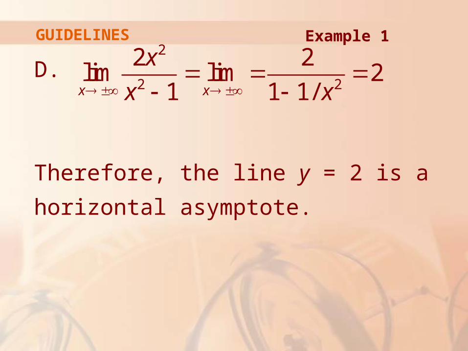
D.

Therefore, the line y = 2 is a horizontal

asymptote.

2

2 2

2 2lim lim 2

1 1 1/x x

x

x x

Example 1

GUIDELINES

Since the denominator is 0 when x = ±1,

we compute the following limits:

Thus, the lines x = 1 and x = -1 are vertical asymptotes.

2 2

2 21 1

2 2

2 21 1

2 2lim lim

1 1

2 2lim lim

1 1

x x

x x

x x

x x

x x

x x

Example 1

GUIDELINES

This information about

limits and asymptotes

enables us to draw the

preliminary sketch,

showing the parts of the

curve near the

asymptotes.

Example 1

GUIDELINES

E.

Since f’(x) > 0 when x < 0 (x ≠ 1) and f’(x) < 0

when x > 0 (x ≠ 1), f is:

Increasing on (-∞, -1) and (-1, 0)

Decreasing on (0, 1) and (1, ∞)

2 2

2 2 2 2

4 ( 1) 2 2 4'( )

( 1) ( 1)

x x x x xf x

x x

Example 1

GUIDELINES

F. The only critical number is x = 0.

Since f’ changes from positive to negative

at 0, f(0) = 0 is a local maximum by the First

Derivative Test.

Example 1

GUIDELINES

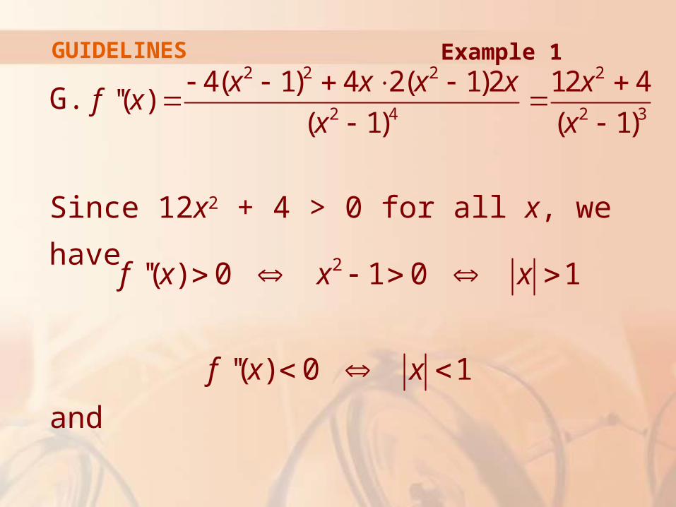
G.

Since 12x2 + 4 > 0 for all x, we have

and

2 2 2 2

2 4 2 3

4( 1) 4 2( 1)2 12 4''( )

( 1) ( 1)

x x x x xf x

x x

2''( ) 0 1 0 1f x x x

''( ) 0 1f x x

Example 1

GUIDELINES

Thus, the curve is concave upward on

the intervals (-∞, -1) and (1, ∞) and concave

downward on (-1, -1).

It has no point of inflection since 1 and -1

are not in the domain of f.

Example 1

GUIDELINES

H. Using the

information in E–G,

we finish the sketch.

Example 1

GUIDELINES

Sketch the graph of:2

( )1

xf x

x

Example 2

A. Domain = {x | x + 1 > 0}

= {x | x > -1}

= (-1, ∞)


C. Symmetry: None


GUIDELINES

D. Since , there is no horizontal

asymptote.

Since as x → -1+ and f(x) is

always positive, we have ,

and so the line x = -1 is a vertical asymptote

2

lim1x

x

x

2

1lim

1x

x

x

Example 2

1 0x

GUIDELINES

E.

We see that f’(x) = 0 when x = 0 (notice that

-4/3 is not in the domain of f).

So, the only critical number is 0.

2

3/ 2

2 1 1/(2 1) (3 4)'( )

1 2( 1)

x x x x x xf x

x x

Example 2

GUIDELINES

As f’(x) < 0 when -1 < x < 0 and f’(x) > 0

when x > 0, f is:

Decreasing on (-1, 0)

Increasing on (0, ∞)

Example 2

GUIDELINES

F. Since f’(0) = 0 and f’ changes from

negative to positive at 0, f(0) = 0 is

a local (and absolute) minimum by

the First Derivative Test.

Example 2

GUIDELINES

G.

Note that the denominator is always positive.

The numerator is the quadratic 3x2 + 8x + 8, which is always positive because its discriminant is b2 - 4ac = -32, which is negative, and the coefficient of x2 is positive.

3/ 2 2 1/ 2

3

2

5/ 2

2( 1) (6 4) (3 4)3( 1)''( )

4( 1)

3 8 8

4( 1)

x x x xf x

x

x x

x

Example 2

So, f”(x) > 0 for all x in the domain of f.

This means that:

f is concave upward on (-1, ∞).

There is no point of inflection.


GUIDELINES

H. The curve is

sketched here.

Example 2

GUIDELINES

Sketch the graph of:

f(x) = xex

Example 3

A. The domain is .


C. Symmetry: None


GUIDELINES

D. As both x and ex become large as

x → ∞, we have

However, as x → -∞, ex → 0.

lim x

xxe

Example 3

So, we have an indeterminate product that

requires the use of l’Hospital’s Rule:

Thus, the x-axis is a horizontal asymptote.

1lim lim lim lim ( )

0

x xx xx x x x

xxe e

e e


GUIDELINES

E. f’(x) = xex + ex = (x + 1) ex

As ex is always positive, we see that f’(x) > 0

when x + 1 > 0, and f’(x) < 0 when x + 1 < 0.

So, f is: Increasing on (-1, ∞)

Decreasing on (-∞, -1)

Example 3

GUIDELINES

F. Since f’(-1) = 0 and f’ changes

from negative to positive at x = -1,

f(-1) = -e-1 is a local (and absolute)

minimum.

Example 3

GUIDELINES

G. f’’(x) = (x + 1)ex + ex = (x + 2)ex

f”(x) = 0 if x > -2 and f’’(x) < 0 if x < -2.

So, f is concave upward on (-2, ∞) and concave downward on (-∞, -2).

The inflection point is (-2, -2e-2)

Example 3

GUIDELINES

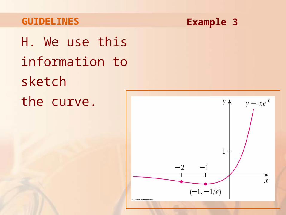
H. We use this

information to sketch

the curve.

Example 3

GUIDELINES

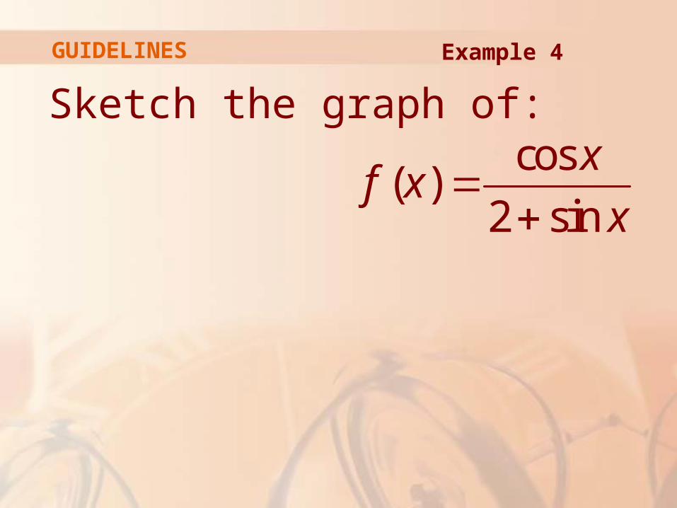
Sketch the graph of:cos

( )2 sin

xf x

x

Example 4

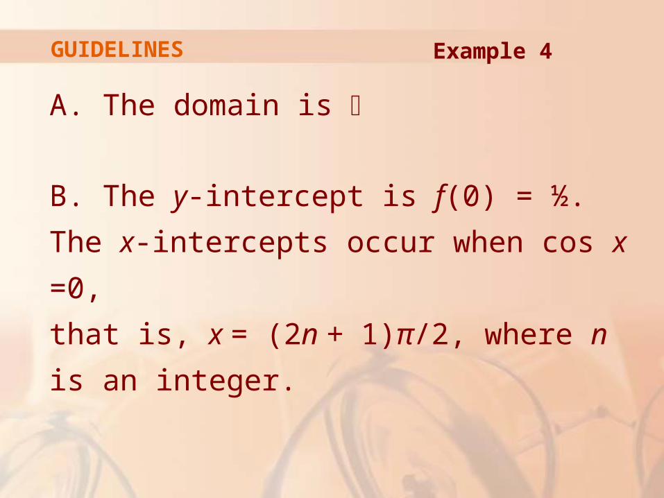
A. The domain is

B. The y-intercept is f(0) = ½.

The x-intercepts occur when cos x =0,

that is, x = (2n + 1)π/2, where n is an integer.


GUIDELINES

C. f is neither even nor odd.

However, f(x + 2π) = f(x) for all x.

Thus, f is periodic and has period 2π.

So, in what follows, we need to consider only 0 ≤ x ≤ 2π and then extend the curve by translation in part H.

D. Asymptotes: None

Example 4

GUIDELINES

E.

Thus, f’(x) > 0 when 2 sin x + 1 < 0

sin x < -½ 7π/6 < x < 11π/6

2

2

(2 sin )( sin ) cos (cos )'( )

(2 sin )

2sin 1

(2 sin )

x x x xf x

x

x

x

Example 4

Thus, f is:

Increasing on (7π/6, 11π/6)

Decreasing on (0, 7π/6) and (11π/6, 2π)


GUIDELINES

F. From part E and the First Derivative

Test, we see that:

The local minimum value is f(7π/6) = -1/

The local maximum value is f(11π/6) = -1/

3

Example 4

3

GUIDELINES

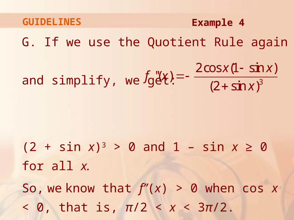
G. If we use the Quotient Rule again

and simplify, we get:

(2 + sin x)3 > 0 and 1 – sin x ≥ 0 for all x.

So, we know that f’’(x) > 0 when cos x < 0,

that is, π/2 < x < 3π/2.

3

2cos (1 sin )''( )

(2 sin )

x xf x

x

Example 4

Thus, f is concave upward on (π/2, 3π/2)

and concave downward on (0, π/2) and

(3π/2, 2π).

The inflection points are (π/2, 0) and

(3π/2, 0).


GUIDELINES

H. The graph of the

function restricted

to 0 ≤ x ≤ 2π is shown

here.

Example 4

GUIDELINES

Then, we extend it,

using periodicity,

to the complete graph

here.

Example 4

GUIDELINES

Sketch the graph of:

y = ln(4 - x2)

Example 5

A. The domain is:

{x | 4 − x2 > 0} = {x | x2 < 4}

= {x | |x| < 2}

= (−2, 2)


GUIDELINES

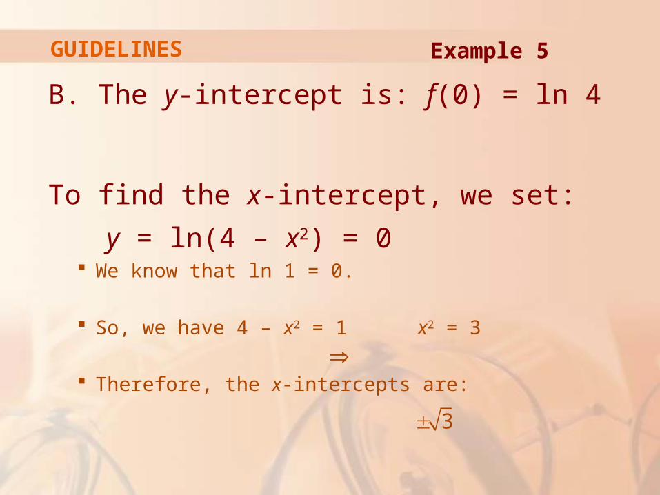
B. The y-intercept is: f(0) = ln 4

To find the x-intercept, we set:

y = ln(4 – x2) = 0 We know that ln 1 = 0.

So, we have 4 – x2 = 1 x2 = 3

Therefore, the x-intercepts are:

Example 5

3

GUIDELINES

C. f(-x) = f(x)

Thus,

f is even.

The curve is symmetric about the y-axis.

Example 5

GUIDELINES

D. We look for vertical asymptotes

at the endpoints of the domain.

Since 4 − x2 → 0+ as x → 2- and as x → 2+, we have:

Thus, the lines x = 2 and x = -2 are vertical asymptotes.

2 2

2 2lim ln(4 ) lim ln(4 )x x

x x

Example 5

GUIDELINES

E.

f’(x) > 0 when -2 < x < 0 and f’(x) < 0 when

0 < x < 2.

So, f is: Increasing on (-2, 0) Decreasing on (0, 2)

2

2'( )

4

xf x

x

Example 5

GUIDELINES

F. The only critical number is x = 0.

As f’ changes from positive to negative at 0,

f(0) = ln 4 is a local maximum by the First

Derivative Test.

Example 5

GUIDELINES

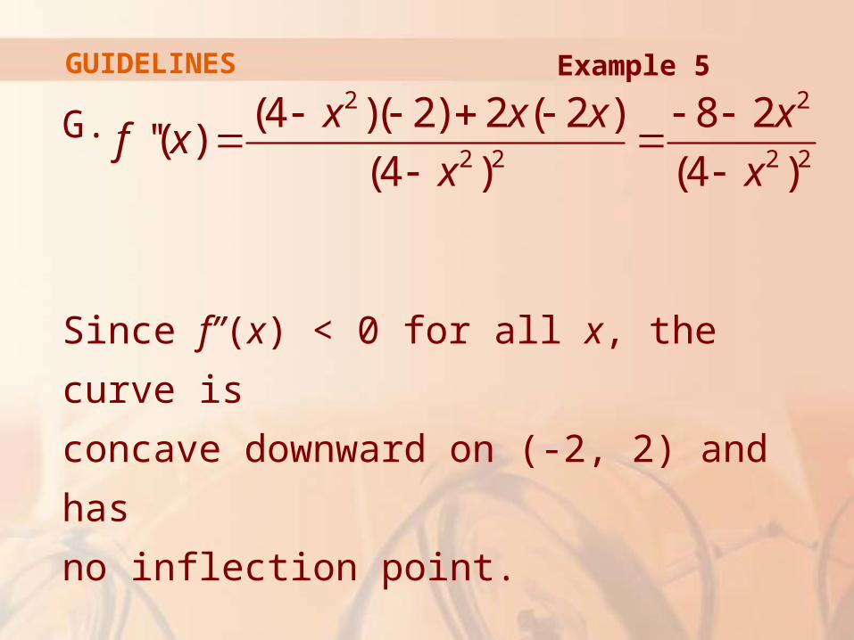
G.

Since f”(x) < 0 for all x, the curve is

concave downward on (-2, 2) and has

no inflection point.

2 2

2 2 2 2

(4 )( 2) 2 ( 2 ) 8 2''( )

(4 ) (4 )

x x x xf x

x x

Example 5

GUIDELINES

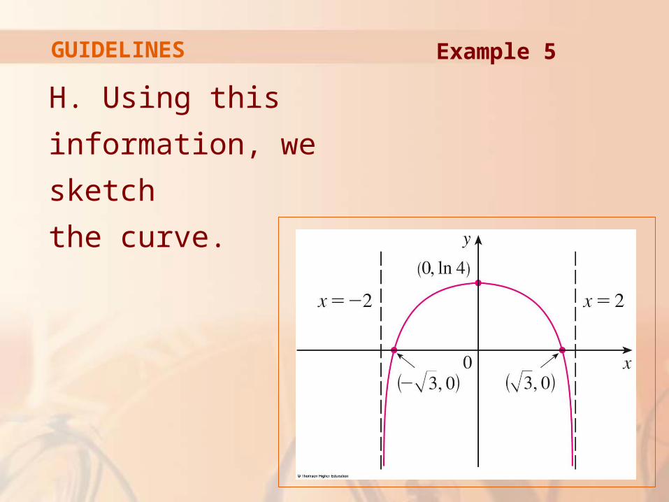
H. Using this

information, we

sketch

the curve.

Example 5

SLANT ASYMPTOTES

Some curves have asymptotes that

are oblique—that is, neither horizontal

nor vertical.

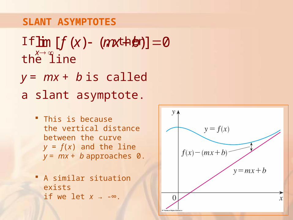
SLANT ASYMPTOTES

If

, then the line

y = mx + b is called a

slant asymptote.

This is because the vertical distance between the curve y = f(x) and the line y = mx + b approaches 0.

A similar situation exists if we let x → -∞.

lim[ ( ) ( )] 0x

f x mx b

SLANT ASYMPTOTES

For rational functions, slant asymptotes occur

when the degree of the numerator is one more

than the degree of the denominator.

In such a case, the equation of the slant asymptote can be found by long division—as in following example.

SLANT ASYMPTOTES

Sketch the graph of:3

2( )

1

xf x

x

Example 6

A. The domain is: = (-∞, ∞)


C. As f(-x) = -f(x), f is odd and its graph is

symmetric about the origin.

Example 6SLANT ASYMPTOTES

SLANT ASYMPTOTES

Since x2 + 1 is never 0, there is no vertical

asymptote.

Since f(x) → ∞ as x → ∞ and f(x) → -∞ as

x → - ∞, there is no horizontal asymptote.

Example 6

SLANT ASYMPTOTES

However, long division gives:

So, the line y = x is a slant asymptote.

3

2 2( )

1 1

x xf x x

x x

2

2

1

( ) 0 as11 1

x xf x x xx

x

Example 6

SLANT ASYMPTOTES

E.

Since f’(x) > 0 for all x (except 0), f is

increasing on (- ∞, ∞).

2 2 3 2 2

2 2 2 2

3 ( 1) 2 ( 3)'( )

( 1) ( 1)

x x x x x xf x

x x

Example 6

SLANT ASYMPTOTES

F. Although f’(0) = 0, f’ does not

change sign at 0.

So, there is no local maximum or minimum.

Example 6

SLANT ASYMPTOTES

G.

Since f’’(x) = 0 when x = 0 or x = ± , we set up the following chart.

3 2 2 4 2 2

2 4

2

2 3

(4 6 )( 1) ( 3 ) 2( 1)2''( )

( 1)

2 (3 )

( 1)

x x x x x x xf x

x

x x

x

Example 6

3

SLANT ASYMPTOTES

The points of

inflection are:

(− , −¾ )

(0, 0)

( , ¾ )

3 3

3 3

Example 6

SLANT ASYMPTOTES

H. The graph of f is

sketched.

Example 6

applications of differentiation

Documents