Master Thesis

Software Engineering

Thesis no: MSE-2007:20

August 2007

School of EngineeringBlekinge Institute of TechnologyBox 520SE – 372 25 RonnebySweden

Applications of data mining algorithms

to analysis of medical data

Dariusz Matyja

This thesis is submitted to the School of Engineering at Blekinge Institute of Technology inpartial fulfillment of the requirements for the degree of Master of Science in SoftwareEngineering. The thesis is equivalent to 20 weeks of full time studies.

Contact Information:

Author:Dariusz MatyjaE-mail: mneman@tlen.pl

University advisors:Lech Tuzinkiewicz, PhD.Institute of Applied InformaticsWrocław University of Technology, Poland

Niklas LavessonSchool of EngineeringBlekinge Institute of Technology, Sweden

School of EngineeringBlekinge Institute of TechnologyBox 520SE – 372 25 RonnebySweden

Internet : www.bth.se/tekPhone : +46 457 38 50 00Fax : + 46 457 271 25

ii

ABSTRACT

Medical datasets have reached enormous capacities.This data may contain valuable information that awaitsextraction. The knowledge may be encapsulated invarious patterns and regularities that may be hidden inthe data. Such knowledge may prove to be priceless infuture medical decision making. The data which isanalyzed comes from the Polish National Breast CancerPrevention Program ran in Poland in 2006.

The aim of this master's thesis is the evaluation ofthe analytical data from the Program to see if thedomain can be a subject to data mining. The next step isto evaluate several data mining methods with respect totheir applicability to the given data. This is to showwhich of the techniques are particularly usable for thegiven dataset. Finally, the research aims at extractingsome tangible medical knowledge from the set.

The research utilizes a data warehouse to store thedata. The data is assessed via the ETL process. Theperformance of the data mining models is measuredwith the use of the lift charts and confusion(classification) matrices. The medical knowledge isextracted based on the indications of the majority of themodels. The experiments are conducted in theMicrosoft SQL Server 2005.

The results of the analyses have shown that theProgram did not deliver good-quality data. A lot ofmissing values and various discrepancies make itespecially difficult to build good models and draw anymedical conclusions. It is very hard to unequivocallydecide which is particularly suitable for the given data.It is advisable to test a set of methods prior to theirapplication in real systems.

The data mining models were not unanimous aboutpatterns in the data. Thus the medical knowledge is notcertain and requires verification from the medicalpeople. However, most of the models stronglyassociated patient's age, tissue type, hormonal therapiesand disease in family with the malignancy of cancers.

The next step of the research is to present thefindings to the medical people for verification. In thefuture the outcomes may constitute a good backgroundfor development of a Medical Decision SupportSystem.

Keywords: medical data mining, medical datawarehouse, medical data, breast cancer.

1

Contents

1 INTRODUCTION...............................................................................................................................7

1.1 RESEARCH AIM AND OBJECTIVES...........................................................................................................81.2 RESEARCH QUESTIONS.........................................................................................................................81.3 RESEARCH METHODOLOGY...................................................................................................................91.4 THESIS OUTLINE.................................................................................................................................9

2 RELATED WORK............................................................................................................................11

3 DATA MINING METHODS...........................................................................................................14

3.1 DECISION TREES..............................................................................................................................183.2 ASSOCIATION RULES.........................................................................................................................193.3 CLUSTERING....................................................................................................................................203.4 NAIVE BAYES..................................................................................................................................213.5 ARTIFICIAL NEURAL NETWORKS.........................................................................................................213.6 LOGISTIC REGRESSION.......................................................................................................................22

4 IMPLEMENTATION OF THE DATA MINING METHODS IN THE MICROSOFT BI SQL

SERVER 2005 ......................................................................................................................................24

4.1 MICROSOFT ASSOCIATION RULES.......................................................................................................254.2 MICROSOFT DECISION TREES.............................................................................................................264.3 MICROSOFT CLUSTERING...................................................................................................................274.4 MICROSOFT NAIVE BAYES................................................................................................................284.5 MICROSOFT NEURAL NETWORK.........................................................................................................284.6 MICROSOFT LOGISTIC REGRESSION.....................................................................................................30

5 SOURCES OF THE ANALYTICAL DATA..................................................................................31

5.1 POLISH NATIONAL BREAST CANCER PREVENTION PROGRAM..................................................................315.2 DATA RECEPTION..............................................................................................................................33

6 ANALYTICAL DATA PREPARATION.......................................................................................34

6.1 INTRODUCTION TO DATA WAREHOUSE MODELING....................................................................................346.2 MEDICAL DATA WAREHOUSE MODEL....................................................................................................356.3 ETL PROCESS..................................................................................................................................386.4 QUALITY ISSUES...............................................................................................................................39

7 DATA ANALYSES...........................................................................................................................41

7.1 DATA PRE-ANALYSES........................................................................................................................417.2 INITIAL FEATURE SELECTION...............................................................................................................527.3 DESCRIPTION OF THE EXPERIMENT.......................................................................................................537.4 MICROSOFT DECISION TREES.............................................................................................................537.5 MICROSOFT CLUSTERING...................................................................................................................597.6 MICROSOFT NEURAL NETWORK.........................................................................................................657.7 MICROSOFT LOGISTIC REGRESSION.....................................................................................................697.8 MICROSOFT NAIVE BAYES................................................................................................................737.9 MICROSOFT ASSOCIATION RULES.......................................................................................................777.10 EVALUATION OF THE ALGORITHMS.....................................................................................................807.11 CONCLUSIONS FROM THE EVALUATION...............................................................................................84

8 MEDICAL KNOWLEDGE GAINED............................................................................................87

8.1 DECISION TREES...............................................................................................................................878.2 CLUSTERING....................................................................................................................................898.3 NEURAL NETWORK............................................................................................................................918.4 LOGISTIC REGRESSION.......................................................................................................................938.5 ASSOCIATION RULES..........................................................................................................................948.6 NAIVE BAYES..................................................................................................................................968.7 GENERALIZATION OF THE KNOWLEDGE...............................................................................................101

2

9 CONCLUSIONS AND FUTURE WORK....................................................................................102

10 REFERENCES..............................................................................................................................105

3

Index of TablesTABLE 3.1. SAMPLE CLASSIFICATION MATRIX..................................................................................................16TABLE 4.1. PARAMETERS OF THE MICROSOFT ASSOCIATION RULES...................................................................26TABLE 4.2. MICROSOFT DECISION TREES PARAMETERS....................................................................................27TABLE 4.3. MICROSOFT CLUSTERING PARAMETERS..........................................................................................27TABLE 4.4. MICROSOFT NAIVE BAYES PARAMETERS.......................................................................................28TABLE 4.5. MICROSOFT NEURAL NETWORK..................................................................................................29TABLE 7.1. INITIAL FEATURE SELECTION........................................................................................................52TABLE 7.2. CLASSIFICATION MATRIX OF THE DECISION TREE WITH THE ENTROPY SCORE METHOD............................55TABLE 7.3. CLASSIFICATION MATRIX FOR THE BK2 TREE................................................................................55TABLE 7.4. CLASSIFICATION MATRIX FOR THE BDEU TREE.............................................................................56TABLE 7.5. TRUE CLASS VALUES RATES DELIVERED BY THE DECISION TREES MODELS............................................56TABLE 7.6. CLASSIFICATION MATRIX FOR THE EM CLUSTERS...........................................................................61TABLE 7.7. CLASSIFICATION MATRIX FOR THE K-MEANS CLUSTERING..................................................................62TABLE 7.8. TRUE CLASS VALUES RATES DELIVERED BY THE CLUSTERING MODELS.................................................63TABLE 7.9. CLASSIFICATION MATRIX FOR THE 30% SPLIT NEURAL NETWORK......................................................66TABLE 7.10. CLASSIFICATION MATRIX FOR THE 60% SPLIT NEURAL NETWORK....................................................66TABLE 7.11. TRUE CLASS VALUES RATES DELIVERED BY THE NEURAL NETWORKS MODELS.....................................66TABLE 7.12. CLASSIFICATION MATRIX FOR THE 30% SPLIT LOGISTIC REGRESSION................................................70TABLE 7.13. CLASSIFICATION MATRIX FOR THE 50% SPLIT LOGISTIC REGRESSION................................................70TABLE 7.14. TRUE CLASS VALUES RATES DELIVERED BY THE LOGISTIC REGRESSION MODEL..................................70TABLE 7.15. CLASSIFICATION MATRIX FOR THE MICROSOFT NAIVE BAYES.........................................................73TABLE 7.16. TRUE CLASS VALUES RATES DELIVERED BY THE NAIVE BAYES MODEL.............................................74TABLE 7.17. CLASSIFICATION MATRIX FOR THE ASSOCIATION RULES...................................................................77TABLE 7.18. TRUE CLASS VALUES RATES DELIVERED BY THE ASSOCIATION RULES MODEL......................................77TABLE 8.1. RULES DERIVED FROM THE ENTROPY DECISION TREE FOR EACH OF THE CLASS VALUE, PROVIDED WITH THE

PROBABILITY OF PREDICTION.........................................................................................................................87TABLE 8.2. DISTRIBUTIONS (AT LEAST 30%) OF CLASS VALUES IN PARTICULAR CLUSTERS....................................90TABLE 8.3. IMPACT OF THE ATTRIBUTES' VALUES ON THE CLASS VALUE FOR THE NEURAL NETWORK........................92TABLE 8.4. IMPACT OF THE ATTRIBUTES' VALUES ON THE CLASS VALUE FOR THE LOGISTIC REGRESSION....................93TABLE 8.5. ITEM SETS WITH THE HIGHEST SUPPORT FOR THE ASSOCIATION RULES.................................................94TABLE 8.6. TOP 30 RULES WITH THE HIGHEST IMPORTANCE AND THE PROBABILITY EQUAL 1..................................94

4

Index of FiguresFIGURE 3.1. SAMPLE LIFT CHART..................................................................................................................17FIGURE 3.2. SAMPLE ROC PLOT..................................................................................................................17FIGURE 3.3. A SITUATION WHEN THE K-MEANS ALGORITHM DOES NOT DELIVER AN OPTIMAL SOLUTION. TWO GRAY

SQUARES DENOTE THE INITIAL CHOICE OF THE CLUSTER CENTERS, DASHED ELLIPSES SHOW THE NATURAL CLUSTERS, THE

SOLID-LINED ONES – THE ACTUAL GROUPING. ..................................................................................................20FIGURE 3.4. LOGIT TRANSFORMATION............................................................................................................23FIGURE 3.5: LOGISTIC REGRESSION FUNCTION.................................................................................................23FIGURE 4.1. SAMPLE LIFT CHART GENERATED BY THE MICROSOFT BI SQL SERVER 2005...................................25FIGURE 5.1. ACTIONS IN THE NATIONAL BREAST CANCER PREVENTION PROGRAM..............................................33FIGURE 6.1. DATA WAREHOUSE CONCEPTUAL MODEL.......................................................................................36FIGURE 6.2. DATA WAREHOUSE LOGICAL MODEL.............................................................................................37FIGURE 6.3. DATA WAREHOUSE PHYSICAL MODEL...........................................................................................38FIGURE 6.4: DATA INTEGRATION PROJECT IN THE MICROSOFT INTEGRATION SERVICES ENVIRONMENT FOR THE DATA

FROM THE BREAST CANCER PREVENTION PROGRAM (THE ETL PROCESS)...........................................................39FIGURE 7.1. DISTRIBUTION OF THE AGE ATTRIBUTE.........................................................................................41FIGURE 7.2. DISTRIBUTION OF THE BIRTHS ATTRIBUTE.....................................................................................42FIGURE 7.3. DISTRIBUTION OF THE CITY ATTRIBUTE........................................................................................42FIGURE 7.4. DISTRIBUTION OF THE FIRSTMENSTRUATION ATTRIBUTE.................................................................43FIGURE 7.5. DISTRIBUTION OF THE LASTMENSTRUATION ATTRIBUTE..................................................................43FIGURE 7.6. DISTRIBUTION OF THE HORMONALTHERAPIESEARLIER ATTRIBUTE....................................................44FIGURE 7.7. DISTRIBUTION OF THE HORMONALTHERAPIESNOW ATTRIBUTE........................................................44FIGURE 7.8. DISTRIBUTION OF THE MAMMOGRAPHIESCOUNT ATTRIBUTE............................................................45FIGURE 7.9. DISTRIBUTION OF THE SELFEXAMINATION ATTRIBUTE....................................................................45FIGURE 7.10: DISTRIBUTION OF THE SYMPTOMDESCRIPTION ATTRIBUTE.............................................................46FIGURE 7.11. DISTRIBUTION OF THE TISSUETYPENAME ATTRIBUTE...................................................................46FIGURE 7.12: DISTRIBUTION OF THE BIRADSDESCRIPTION ATTRIBUTE............................................................47FIGURE 7.13: DISTRIBUTION OF THE BIRADSVALUE ATTRIBUTE....................................................................47FIGURE 7.14. DISTRIBUTION OF THE CHANGECOUNT ATTRIBUTE.......................................................................48FIGURE 7.15. DISTRIBUTION OF THE CHANGESIDE ATTRIBUTE..........................................................................48FIGURE 7.16: DISTRIBUTION OF THE CHANGESIZE ATTRIBUTE...........................................................................49FIGURE 7.17. DISTRIBUTION OF THE CHANGELOCATION ATTRIBUTE...................................................................49FIGURE 7.18: DISTRIBUTION OF THE FAMILYLINE ATTRIBUTE...........................................................................50FIGURE 7.19. DISTRIBUTION OF THE RELATIVE ATTRIBUTE...............................................................................50FIGURE 7.20. DISTRIBUTION OF THE MONTH ATTRIBUTE..................................................................................51FIGURE 7.21. DISTRIBUTION OF THE DIAGNOSISDESCRIPTION ATTRIBUTE, WHICH IS THE CLASS FOR THE INSTANCES. .51FIGURE 7.22. DECISION TREE BUILT WITH THE USE OF THE ENTROPY SCORE METHOD............................................54FIGURE 7.23. DECISION TREE BUILT WITH THE USE OF THE BAYESIAN WITH K2 PRIOR (BK2)..............................55FIGURE 7.24. DECISION TREE BUILT WITH THE USE OF THE BAYESIAN DIRICHLET EQUIVALENT WITH UNIFORM PRIOR

(BDEU)..................................................................................................................................................56FIGURE 7.25. LIFT CHART FOR THE MALIGNANT CLASS FOR THE DECISION TREES.................................................57FIGURE 7.26. LIFT CHART FOR THE SUSPICIOUS CLASS FOR THE DECISION TREES..................................................57FIGURE 7.27. LIFT CHART FOR THE PROBABLYMILD CLASS FOR THE DECISION TREES...........................................58FIGURE 7.28. LIFT CHART FOR THE MILD CLASS FOR THE DECISION TREES..........................................................58FIGURE 7.29: LIFT CHART FOR THE NORM CLASS FOR THE DECISION TREES.........................................................59FIGURE 7.30. CLUSTERS GENERATED WITH THE USE OF THE EM ALGORITHM......................................................60FIGURE 7.31. DISTRIBUTION OF CLASS VALUES IN INDIVIDUAL EM CLUSTERS.....................................................60FIGURE 7.32. CLUSTERS GENERATED WITH THE USE OF THE K-MEANS ALGORITHM...............................................61FIGURE 7.33. DISTRIBUTION OF THE CLASS VALUES IN INDIVIDUAL K-MEANS CLUSTERS.........................................62FIGURE 7.34. LIFT CHART FOR THE MALIGNANT CLASS VALUE FOR CLUSTERS.....................................................63FIGURE 7.35. LIFT CHART FOR THE SUSPICIOUS CLASS VALUE FOR CLUSTERS.......................................................63FIGURE 7.36. LIFT CHART FOR THE PROBABLYMILD CLASS VALUE FOR CLUSTERS................................................64FIGURE 7.37. LIFT CHART FOR THE MILD CLASS VALUE FOR CLUSTERS...............................................................64FIGURE 7.38. LIFT CHART FOR THE NORM CLASS VALUE FOR CLUSTERS..............................................................65FIGURE 7.39. LIFT CHART FOR THE MALIGNANT CLASS VALUE FOR NEURAL NETWORKS........................................67FIGURE 7.40. LIFT CHART FOR THE SUSPICIOUS CLASS VALUE FOR NEURAL NETWORKS..........................................67FIGURE 7.41. LIFT CHART FOR THE PROBABLYMILD CLASS VALUE FOR NEURAL NETWORKS...................................68FIGURE 7.42. LIFT CHART FOR THE MILD CLASS VALUE FOR NEURAL NETWORKS.................................................68

5

FIGURE 7.43. LIFT CHART FOR THE NORM CLASS VALUE FOR NEURAL NETWORKS................................................69FIGURE 7.44. LIFT CHART FOR THE MALIGNANT CLASS VALUE FOR LOGISTIC REGRESSION.....................................71FIGURE 7.45. LIFT CHART FOR THE SUSPICIOUS CLASS VALUE FOR LOGISTIC REGRESSION.......................................71FIGURE 7.46. LIFT CHART FOR THE PROBABLYMILD CLASS VALUE FOR LOGISTIC REGRESSION................................72FIGURE 7.47. LIFT CHART FOR THE MILD CLASS VALUE FOR LOGISTIC REGRESSION..............................................72FIGURE 7.48. LIFT CHART FOR THE NORM CLASS VALUE FOR LOGISTIC REGRESSION..............................................73FIGURE 7.49. LIFT CHART FOR THE MALIGNANT CLASS VALUE FOR NAÏVE BAYES...............................................74FIGURE 7.50. LIFT CHART FOR THE SUSPICIOUS CLASS VALUE FOR NAÏVE BAYES................................................75FIGURE 7.51. LIFT CHART FOR THE PROBABLYMILD CLASS VALUE FOR NAÏVE BAYES.........................................75FIGURE 7.52. LIFT CHART FOR THE MILD CLASS VALUE FOR NAÏVE BAYES........................................................76FIGURE 7.53. LIFT CHART FOR THE NORM CLASS VALUE FOR NAÏVE BAYES.......................................................76FIGURE 7.54. LIFT CHART FOR THE MALIGNANT CLASS VALUE FOR ASSOCIATION RULES........................................78FIGURE 7.55. LIFT CHART FOR THE SUSPICIOUS CLASS VALUE FOR ASSOCIATION RULES.........................................78FIGURE 7.56. LIFT CHART FOR THE PROBABLYMILD CLASS VALUE FOR ASSOCIATION RULES..................................79FIGURE 7.57. LIFT CHART FOR THE MILD CLASS VALUE FOR ASSOCIATION RULES.................................................79FIGURE 7.58. LIFT CHART FOR THE NORM CLASS VALUE FOR ASSOCIATION RULES................................................80FIGURE 7.59. COMPARISON OF THE CLASSIFICATION MATRICES OF ALL THE MODELS..............................................81FIGURE 7.60. COMPARATIVE LIFT CHART OF ALL OF THE MODELS WITH RESPECT TO THE MALIGNANT CLASS VALUE. .81FIGURE 7.61. COMPARATIVE LIFT CHART OF ALL OF THE MODELS WITH RESPECT TO THE SUSPICIOUS CLASS VALUE. . .82FIGURE 7.62. COMPARATIVE LIFT CHART OF ALL OF THE MODELS WITH RESPECT TO THE PROBABLYMILD CLASS VALUE

................................................................................................................................................................83FIGURE 7.63. COMPARATIVE LIFT CHART OF ALL OF THE MODELS WITH RESPECT TO THE MILD CLASS VALUE...........83FIGURE 7.64. COMPARATIVE LIFT CHART OF ALL OF THE MODELS WITH RESPECT TO THE NORM CLASS VALUE..........84FIGURE 8.1. THE MALIGNANT CLASS VALUE CHARACTERISTICS FOR THE NAÏVE BAYES........................................96FIGURE 8.2. THE SUSPICIOUS CLASS VALUE CHARACTERISTICS FOR THE NAÏVE BAYES..........................................97FIGURE 8.3. THE PROBABLYMILD CLASS VALUE CHARACTERISTICS FOR THE NAÏVE BAYES...................................98FIGURE 8.4. THE MILD CLASS VALUE CHARACTERISTICS FOR THE NAÏVE BAYES.................................................99FIGURE 8.5. THE NORM CLASS VALUE CHARACTERISTICS FOR THE NAÏVE BAYES...............................................100

6

1 INTRODUCTION

Health care institutions all over the world have been gathering medical data overthe years of their operation. The enormous volume of this data is getting to a point where itwill exceed available storage capacities [8]. This data may constitute a valuable sourceof medical information that has potential to be very useful in diagnosing and treatment.Its format, however, may require some additional processing before the data can servedoctors as a precious source of information in their everyday work. This data may comprisethousands of records which may contain valuable patterns and dependencies hidden deepamong them. The volume of the dataset and complexity of the medical domain make it verydifficult for a human to analyze the data manually to extract hidden information. For thisreason the computer science proves to be helpful. Machines are used to mine datafor patterns and regularities. Various data mining algorithms have been developedwhich analyze the data in order to extract underlying knowledge [23], [31].

This research is focused on breast cancer. According to [2] this disease is the mostfrequent malignant cancer in Polish women (about 20% of all malignant cancers). In year2000 almost 11 000 women in Poland suffered from the disease. The number grewcomparing to year 1999 and prognoses for the future are pessimistic. It is estimatedthat mortality rate due to the breast cancer increases about 0.7% every year. This wasthe reason for the president of the Polish National Health Fund (Polish: Narodowy Fundusz

Zdrowia, NFZ) to issue a disposition [2] in 2005 to start (among others) the Breast CancerPrevention Program (described in details in the Chapter 5).

The etiology of the breast cancer, despite broad and thorough research conductedby leading oncological institutions all over the world, is still not well known [2]. The diseasecan be induced by a variety of factors (carcinogens) such as mutations of genes, age,occurrences of the disease in family, and many others. However, the best results in treatmentare achieved when the disease is diagnosed early enough. Otherwise costs are incomparablygreater. They encompass costs of treatment (operations, radiology, chemotherapy, etc),complications, sick leaves, pensions, welfare, and so on. Another problem are the social andpsychological side-effects of the disease and possibly a death in family. All these reasonsconfirm the fact that the sooner the disease has been diagnosed it gives not only a greaterchance for complete cure but also significantly smaller cost at the same time. The Polishgovernment has already introduced several preventive programs concerning the cancer. Theexperiences from the last one (conducted between 1976 and 1990 [2]) allowed for creation ofa model breast cancer screening program and its introduction in the six leading medicalcenters in Poland. In Western European countries and the USA it has been agreed that thebest way to reduce malignant cancer occurrences are national preventive programs sponsoredby governments. They aim not only at diagnosing patients but also purchasing modernequipment, increasing awareness of the society and encouraging people to take better care oftheir health. In these countries such programs helped to decrease mortality rate by up to onethird [2].

The Breast Cancer Prevention Program mentioned above brought a lot of raw datain a form of surveys. Each of them was filled out by both patients and doctors participatingin the screening. The former provided general information about the state of their health andinformation concerning various aspects from their lives (number of births, age at first andlast menstruation, etc.). The latter entered the results of the screening. The data contained inthese surveys may contain valuable information, encapsulated in various patterns andregularities, which could be used in a diagnosing process in the future. To extract theknowledge the data has to be transformed to an electronic form, then cleansed and finallyanalyzed.

7

1.1 Research aim and objectives

The research has three main goals:1. Evaluation of the analytical data gathered from the surveys of the National

Breast Cancer Prevention Program ran in Poland in 2006. The data is assessedin order to see if it may constitute a source for building a data warehouse and datamining models. The research objectives are as follows:a. The ETL process [19] which encompasses extraction of the data from

operational databases (E), data transformations so that it fits the data warehouse(T) and finally loading the data into the warehouse (L).

b. Final assessments of the quality based on the amount of data which had to beremoved because of inconsistencies or missing values.

2. Evaluation of data mining methods with regard to their applicability to the data

from the Program. There are many algorithms and methods that seek for patterns indata. The evaluation of the methods may turn out to be a valuable source ofinformation for medical people who will be responsible for drawing conclusionsfrom the outcomes of the Program. The objectives are as follows:a. Thorough literature survey in order to determine which algorithms are used in

medicine (especially for the breast cancer). This is also to see what performancemetrics are used to evaluate the algorithms.

b. Overview of the methods and their implementation in the analyticalenvironment.

c. Creation of a data warehouse which aggregates the analytical data. d. Generation of data mining models.e. Evaluation of the performance of the models.

3. Extraction of medical knowledge from the dataset. The knowledge is measuredby unanimousness of patterns delivered by the data mining models. Patternsdiscovered by most of them are likely to constitute the hidden informationpotentially useful from the perspective of a diagnosing process. Even though thealgorithms are different in their nature and view the data from different angles whenthey discover similar patterns these findings have to be taken as potentially valuable.The methods can associate certain attributes with each other or not find anyassociations whatsoever. From such findings relevant conclusions can be drawn. Thediversity of the methods is actually an advantage in this research. The objectives areas follows:a. Extraction of patterns from individual models.b. Generalization of the knowledge.

1.2 Research questionsThere are three research questions of this study:

1. What is the quality of the medical dataset gathered from the Polish National Breast

Cancer Prevention Program?

The quality of the data in this context denotes consistency of the values in the set(conformance to allowable ranges and formats), the amount of missing values, number ofpossible classes and distribution of the attributes' values.

2. Which data mining methods can be applied to extract knowledge from the medical

dataset gathered from the Polish National Breast Cancer Prevention Program?

The evaluation is based on performance of the methods for the given dataset.

8

3. What knowledge (patterns) can the methods extract from the medical dataset

gathered from the Polish Breast Cancer Prevention Program?

As mentioned previously the validity of the knowledge is measured withunanimousness of patterns discovered by the algorithms.

1.3 Research methodology

There are many classifications of research. Dawson in [11] distinguishes an evaluationproject, i.e. a project which involves evaluation. In the case of this thesis the subject for theevaluation will be the very analytical data and the data mining methods. Thus this study canbe categorized as an evaluation project. Another categorization of projects has beenpresented by Creswell [10] who identified three types of research: qualitative, quantitativeand mixed. The first type of research aims at analyzing qualitative aspects of the studieddomain, i.e. answers a question “what”. It bases on discovering constituent parts andinterrelations among them. It also delivers various interpretations of different aspects. On theother hand there are quantitative studies. They, in turn aim at describing and analyzing factsin a quantitative manner, i.e. representing them in various breakdowns and calculations.They answer a question “how much” or “how many”. The research presented within thisthesis can be thus characterized as a combination of both types. The evaluation of the qualityof the analytical data is done with the use of the quantitative approach. The particularattributes are analyzed in terms of quantities of values. This approach has also been appliedfor the extraction of medical knowledge: indication of majority of data mining models.Qualitative approach is employed for the evaluation of the data mining methods. Hereparticular features of them are analyzed. Also the interrelations among the attributes aretaken into consideration.

A thorough and comprehensive literature study is carried out prior to thedevelopmental and analytical work. The literature encompasses peer-reviewed articles,journals and books. First, the analysis of the data mining algorithms and their applicability tothe breast cancer set is done. Afterwards, a data warehouse is designed and filled with thedata from the Breast Cancer Prevention Program. This step includes an assessment of thequality of the data. Then, the studied data mining methods are applied to the warehouse.Finally, the indications of the data mining models obtained in the previous phase are used togeneralize the knowledge extracted from the dataset.

The research aims at delivering the following outcomes:– evaluation of the medical dataset in terms of quality of the data from the Program,– evaluation of data mining methods with respect to their applicability to the data from the

Program, – knowledge extracted from the dataset.

1.4 Thesis outline

The paper is organized as follows:

Chapter 1 provides an introduction to the topic of the thesis describing the problem that isdiscussed.

Chapter 2 constitutes an overview of the professional literature on topic. Here variousaspects of medical data mining have been mentioned.

In Chapter 3 several data mining methods have been presented. These methods are usedin the analyses.

9

Chapter 4 shows how the data mining methods are implemented in the Microsoft SQLServer 2005 along with any limitations and constraints which the implementation imposes.

Chapter 5 describes the source of the analytical data, i.e. the National Breast CancerPrevention Program held in Poland.

In Chapter 6 the data from the surveys of the Program is prepared for analysis. Herethe ETL process is described followed by design of a data warehouse, which is going to be abasis for the analyses.

Next, in Chapter 7 the very analyses are presented along with the results. This chapter alsoprovides a detailed description of quality of the dataset followed by various experiments.

Chapter 8 contains medical knowledge extracted from the outcomes of the data miningmodels.

Finally, in Chapter 9 overall conclusions have been conveyed along with perspectives offuture work.

10

2 RELATED WORK

The problem of cancer and the oncology in general has been present in theprofessional literature for a long time. Engineers have been looking for patterns in themedical data trying to deliver some valuable knowledge which may be helpful in diagnosingand treatment. This way the information science plays an important role in increasing thelevel of oncological awareness.

Chen and Hsu [5] in their work proposed an evolutionary approach to mining breastcancer data. Their research is based on a genetic algorithm. They argue that traditional datamining methods deliver only n best-fit rules which are far from being convergent to the bestpossible one. In their approach these rules are generated in an evolutionary manner until allof the training samples have been classified correctly. In the process of learning thealgorithm mines for an extra rule for the misclassified examples, which is expected toincrease the overall accuracy. The authors conclude by saying that their method deliversmuch simpler rules in comparison to those generated by many other algorithms. Theirapproach gives slightly better results than a commercial tool PolyAnalyst [33] used forcomparison. However, the authors do not discuss the over-training problem. It seems thattheir model tends to adjust too much to the training data because it seeks for an extra rulethat fits the particular training data.

A genetic algorithm is only one of the possible ways of exploring the medical data.An alternative approach has been presented by Xiong et.al. [32]. They describe their 5-stepprocess of discovering knowledge in the breast cancer data. It consisted of correlation-basedfeature selection followed by qualitative and quantitative analyses in order to builda decision tree and to generate a set of association rules. The authors also recommendremoval of outliers (data points which lie outside of any natural data groups) to furtherimprove the performance. The experiment delivered a model which was accurate in 90% ofpredictions. The authors conclude that often in order to come up with a good model one hasto build several intermediate ones.

Cancer can be influenced by a variety of carcinogens. These factors can come fromboth internal and external environment of a human body. Authors of the article [21] analyzethe impact of caffeine intake and the race on the invasive breast cancer. In their research theyutilize Bayesian network, then cross tabulation (a method to display joint distribution of twoor more variables) and multinomial logistic regression model. The results of the experimentshow that caffeine intake is strongly associated with ethnicity which in turn affectsmenopausal status. These observations have been then compared with the results ofthe logistic regression analysis. The outcomes confirmed what had been observed in theBayesian network: the menopausal status is of the greatest influence on the risk of the breastcancer. Cross tabulation analysis, however, ultimately proved that caffeine intake does notaffect significantly the breast cancer incidence in the studied population. The authorsconclude by saying that it is difficult to associate various aspects of life with breast cancer.Nevertheless, experiments similar to theirs aim at finding connections between those two andare very important. This premise was the basis for starting the research in this thesis. Thedata which comes from the Program also contains information concerning various aspect oflife along with the medical data. Such a dataset may deliver interesting results by associatingthese two types of data.

From among diverse data mining algorithms artificial neural networks are also used inthe field of medicine. The article [1] describes an evolutionary approach to mining breastcancer data with the use of such a network. The author utilizes the Pareto differentialevolution algorithm augmented with local search for predictions of the breast cancer cases.This approach is then compared and contrasted with the back-propagation algorithm. Theresearcher argues that the latter, due to its drawback of potential of falling into a localminimum, tends to train less accurate networks comparing to the evolutionary approach.Besides that, it suffers from high cost of finding appropriate number of hidden neurons. The

11

evolutionary approach proposed by the author brings in a trade-off between the architectureof the network and its predictive ability. The method proved to be quite accurate on thebreast cancer set. During the experiments the standard deviation of the test error was small,which, according to the author, indicates consistency, stability and accuracy of the method.The method has been compared with the one presented in [13]. It turned out to be little moreaccurate, with much lower standard deviation and with computational time significantlysmaller.

Another use of an artificial neural network has been presented by the authors of thearticle [7]. Their approach has been enriched with multivariate adaptive regression splines(MARS). They present superiority of their approach over traditional ones such as:discriminant analysis, linear regression, artificial neural networks and the MARS itself. TheMARS is a method for finding relationships among variables, utilized here to derive inputsto the network. The hybrid model reached equal prediction accuracy as a regular back-

propagation network (without MARS). However, the authors claim that their method isbetter because it identifies only the most important variables.

Authors of the article [12] compare two data mining methods (neural network anddecision trees) and a statistical one (logistic regression) with respect to their applications inmedicine. The experiments proved that the decision trees are the most accurate predictors,with the neural networks to be the second and logistic regression to be the third. These threemethods are also utilized in this thesis to verify their applicability to the data from theProgram. The authors focus also on traditional methods of medical prognosis as a methodwhich encompasses estimations of potential complications and recurrence of the disease. Thetraditional statistical methods: Kaplan-Meier test or Cox-Propositional hazard models arebeing gradually replaced by the data mining techniques and knowledge discovery. Finallythe authors mention several problems and issues that may arise while mining the breastcancer data. First of all is the heterogeneity of the data which constitutes a problem to datamining algorithms. The data can also be incomplete, redundant, inconsistent and imprecise.Thus preparation of the data may require more data reduction than in case of the data fromother types of sources. Such analyses should include all the clinically relevant data and mustmake sense to medical people who will make use of the results. The data in the thesis alsoundergoes the preparation stage within which the ETL process is conducted (Chapter 6). Theauthors conclude that the data mining, being a powerful tool, still requires a human to assessthe results in terms of relevance, applicability and importance of the extracted knowledge.This is also the case in the thesis. The results of the experiments need to be verified by themedical people which will be the next step of the research (beyond the scope of the thesisthough).

Feature selection is another problem that engineers face while mining medical data.Irrelevant attributes may bring noise to the data and harm the prediction abilities ofgenerated models. On the other hand, eradicating important variables also may decrease theaccuracy of the models. This is particularly important in case of the breast cancer data wherea lot of factors can influence occurrence of the disease. The authors of the article [6]compare two methods of selecting the most relevant features (variables) for medical datamining. The first one, data-driven is an automatic approach utilizing automatic mechanisms.The second one is knowledge-driven and bases on opinions of experts. The experimentsshowed that feature selection done by the experts improves sensitivity of a classifier, whileautomated approach improves predictive power on the majority class.

Predictive power of data mining models is very important especially in the medicalfield. It strongly depends on several aspects. One of them is the quality of the training datawhich may have a significant impact on the output model. The data may contain sampleswith values way off in comparison to the rest of them (so-called outliers). The authors of thearticle [24] try to prove that eradicating the outliers makes the set more focused and thusproducing more accurate classifiers. The authors emphasize the need for good criteria uponwhich an instance is judged to be an outlier. They suggest removing the instances that arepredicted differently by different classifiers because. This may mean that such instancescontain contradictory information (not necessarily an error though) and are misleading in the

12

learning process. The experiment revealed that removal of the outliers improved accuracyonly on the training set. On the testing sets the accuracy was either the same or slightlydifferent in both directions (in-plus and in-minus). The authors conclude that since theirmethod does not necessarily improve predictive power of the data mining models it isadvisable to test if the removal of the outliers will do any good to the models. They also saythat even the smallest improvement is of high significance when it comes to the medicaldata. However, the authors used accuracy as the measure of performance of the models. Ithas been proven that accuracy is not a good means for measuring performance of the datamining models, though [25].

Researchers conduct medical analyses in a variety of environments. The authorsof the article [22] evaluated several data mining algorithms implemented in the MicrosoftSQL Server 2005 with respect to their applicability to medical data. Research has shownthat these algorithms have high performance with relatively low errors (type I and type II).The experiments have shown that the best results are gained with the use of the Naive Bayes,artificial neural networks and logistic regression. The worst results were gained by theassociation rules. This article constitutes a baseline for the analyses conducted within thisthesis.

Another aspect that is broadly discussed in the professional literature is the uniquenessof the medical data. The authors of the article [8] list several aspects that make such dataunique. First of all the data is heterogeneous. It usually is very complex and often isenormous in volume. What adds to the heterogeneity is a variety of interpretations ofdiagnoses and screening results. Almost always they are imprecise. Furthermore the medicaldata is difficult to characterize in a mathematical way and does not have any canonical formof representation. Besides that the uniqueness of medical data results from various ethical,legal and social issues as well. The authors condemn any frivolous use of the data when thereare no relevant benefits expected. While performing the medical data mining a researcherhas to ensure that the results are not publicly used unless verified and validated byprofessionals.

All of the analyses conducted with the use of the data mining and statistical algorithmsare of no use to medical people unless included in an easy-to-use medical decision supportsystem. Authors of the article [27] even claim that breast cancer is an example ofinconsistency because specialists do not have access to valuable medical information andguidelines to strengthen their decisions. Their research aims at providing means for easy andconsistent access to various medical data via a decision support system which incorporatesthe data mining techniques. The research presented in the thesis may also contribute to thismotion by providing the evaluation of the methods which can be then incorporated in suchmedical decision support systems.

The reduction of the variability of physicians' medical decisions has been discussedin the article [17]. The authors argue that a computer system has potential to reducevariability in radiologists' interpretations of mammograms. They briefly describe theirsystem which allowed them to limit the unnecessary biopsies (i.e. those done to patientswithout cancer) significantly. They also managed to reduce the standard deviation of thediagnoses by 47%. The variation was measured by the standard deviation of the ROC curves.The system increased the unanimity of medical diagnoses by 13% to 32%. This study showsthat the computers really are used for medical purposes. The authors also present one of theperformance measures – the ROC curves.

Professional literature broadly treats of mining medical data and proves that thesetechniques can be beneficial from the perspective of future diagnosis and treatment. Thisresearch is also focused on evaluation of several data mining algorithms applied to a real-lifemedical data set concerning the breast cancer. The analytical data undergoes the preparationstage (the ETL process) according to the suggestions of some of the authors [12]. Afterwardsthe data is analyzed with the use of some of the methods described by them [7], [12], [22],[32]. The fact that the data comes from a real source makes the results of the analysescredible. As mentioned by [21] studies which analyze the impact of both the medical andnon-medical data on the occurrence of the disease are important.

13

3 DATA MINING METHODS

Data mining, also known as knowledge discovery in databases (KDD [12], [14]) isdefined as “the extraction of implicit, previously unknown, and potentially usefulinformation from data” [31]. It encompasses a set of processes performed automatically [22],whose task is to discover and extract hidden features (such as: various patterns, regularitiesand anomalies) from large datasets. Usually the volume of such sets makes manual analysesat least arduous. All of the data mining processes are conducted with the use of machines,namely computers.

Research fields such as statistics and machine learning contributed greatly to thedevelopment of various data mining and knowledge discovery algorithms. The objectives ofthese algorithms include (among others) pattern recognition, prediction, association andgrouping [31]. They can be applied to a variety of learning problems. Their applicabilityvaries, though. Some of them may give better results in one type of problems in which othersgive worse, or even fail. Some give good results in case of well structured data, whileperforming poor on heterogeneous datasets. Some work only on discrete data, others requireit to be numeric (continuous), etc. Specific features make particular algorithms especiallysuitable for certain domains, for instance association rules are often used for market basketanalysis [28], Naive Bayes is applicable to documents classification [31], others have moregeneric applications. As mentioned in the Chapter 2 the medical datasets are unique in theirnature. They are heterogeneous and contain both discrete and continuous values.

There are several tasks of learning [31]:– classification – an algorithm is given a set of examples that belong to certain predefined

and discrete classes from which it is expected to learn to classify future instances,– regression (numeric prediction) – an algorithm is expected to predict a numeric class

instead of a discrete,– association – an algorithm seeks for any correlations (dependencies) among features,– clustering – an algorithm groups examples that are in some way similar.

Classification and regression are commonly referred to as prediction. They represent aso-called supervised learning [31]. The supervision can be understood by observing the wayin which an algorithm learns. It is given a set of instances, each provided with an outcome(class). The method operates as if it was supervised by this training set telling it what classshould be assigned to a particular instance.

Unlike the prediction, the association learning looks for potentially interestingdependencies among variables. Prediction differs from association learning in two aspects[31]. First of all the latter can be used to predict any attribute of an instance (not just a class).Furthermore it is possible to employ the association to predict more than one attribute at atime.

The clustering, in turn, is used primarily to group instances [31]. It is often applied todatasets in which a class is nonexistent or irrelevant from the perspective of knowledge.However, the method can also be used for classification purposes to determine a missingvalue of an attribute of an instance by assigning it to one of the clusters. Each cluster groupsinstances that are in some way similar or related to each other. The division criteriondepends on a problem and can be distance-based or probability-based. Evaluation of thegroups is usually subjective and depends on how useful a particular division is to a user [31].

The aim of the learning process is to determine a description of a class [31], i.e. thething (value) the algorithm is expected to learn. The process is based on training data fromwhich an algorithm is to gain knowledge by analyzing training examples (or instances) [31].Each instance represents a single independent example of the class. In order to ensure theindependence of the instances the original dataset often has to be denormalized.

All of the instances are characterized by a set of predefined features (attributes), fixedacross the entire dataset [31]. Each of them can bear a value from a certain domain. The factof all of the instances being the same as far as their features go imposes several limitations.

14

For instance some attributes may not apply to certain cases but still have to be there. Anotherproblem are interdependencies among the attributes. A feature type of cancer depends on avalue of an attribute diagnosis as an example.

The attributes can hold several types of values. The following list describes thepossibilities [31]:– numeric values are often referred to as continuous (but not in the mathematical sense).

All the mathematical calculations apply (summation, multiplication, division), forinstance cost,

– nominal attributes take values from a predefined, finite set of possibilities. They oftenrepresent names (labels). Any ordering, distance measuring or any other mathematicalcalculations (such as summation, multiplication, division, etc.) simply do not make senseand usually are not possible. For instances, it is not possible to sum the values of adiagnosis.

– ordinal quantities, which represent sortable labels, for instance temperature hot > mild >cold. Still any mathematical computations are meaningless,

– interval values, which represent sortable numeric attributes which can be arranged inintervals, for instance year. However, still some of the mathematical calculation do notapply here, for instance it does not make sense to sum the years.

The distinction presented is only theoretical and most of the practical applications utilizeonly numeric and nominal types of attributes [31]. Often a special case of nominal values isdistinguished: dichotomy (sometimes referred to as Boolean), which has only two possiblevalues: true and false or yes and no.

The learning process requires some steps to be undertaken prior to building a model.These steps constitute a data preparation stage. Preparation includes gathering the data in oneconsistent dataset. It can either be a delimited flat file, table in a relational database or aspreadsheet. It can also be a data warehouse [31], which is a database storing corporate datain an aggregated, closed-in-time form. The data warehouse often contains historical data,which is rather useless from the perspective of everyday work, but which can be used fordecision making. The past data contains information from which professional people candraw relevant conclusions to support future business decisions. That is why a data warehouseconstitutes a valuable milestone on a way to the data mining [14]. All the steps required inthe process of building a data warehouse are also necessary in the data mining. These includedata reception, cleansing and preparation to deliver a final set of data items ready foranalyses. Also in this research a data warehouse will be built prior to the data mininganalyses. The design of the data warehouse and the steps of the data preparation stage aredescribed in the Chapter 6.

The last important step in the learning process is the verification of the generatedmodel. In order to perform the tests a researcher has to have a separate, preferably disjointwith the training one, set of instances. Obviously there is no sense in testing the model on thetraining data, as this would always give excellent results. On the other hand, usually theamount of data available to build a model is very limited. If the set was split into two subsets(one for training and one for testing) it is highly probable that both would be too little fortheir purposes. The size of the training set strongly affects the quality of the model: thesmaller the set the higher variance of the estimates and thus lower confidence of predictions[31].

The problem of testing sparse datasets has been widely discussed in the professionalliterature [23] and [31]. The engineers seem to agree that today's solution, which is gainingon the acceptance, is the k-fold cross-validation. The method splits the training set into kfolds. Then the algorithm is run k times, each time training the model on the union of k-1subsets and testing it on the remaining k-th one. This process is repeated so that each of thesubsets has been used for testing once. The models obtained in each consecutive iteration arethen combined to create an ultimate result.

The test results are usually expressed in terms of an error. Errors are often presentedwith the use of a classification (or confusion) matrix which presents the “quality” ofpredictions of a data mining model with respect to the class values [31]. A sample matrix for

15

a Boolean problem is presented in the Table 4.1. The matrix shows numbers of correctly andincorrectly predicted instances. It also depicts a class value that was predicted instead of acorrect one. For instance, in the Table 4.1 the value 348 denotes the number of correctlyclassified instances from a class false. In turn, the value 14 denotes the number of instancesfrom the same class which were wrongly classified to the class true. An unquestionablestrength of this method is its simplicity and clarity. It is possible to see at a glance how gooda model is. Such matrices have been used in a variety of data mining situations, includingmedicine [23], [31].

Table 3.1. Sample classification matrix

Actual value false Actual value true

Predicted value false 348 15

Predicted value true 14 208

There are several ways of measuring performance of data mining models. The mostcommon, and the most criticized one is the accuracy [25]. It is computed by applying themodel to a dataset and observing the rate of properly classified instances. It gives goodresults in case of datasets in which the classes are close-to-equally distributed. However, ifone class constitutes an overwhelming majority in the dataset the accuracy may always behigh if the model favors this class. The actual predictive power of such a model for unseenfuture instances may be low, though. Alternative measures include lift charts and area underROC curves (AUC) [31]. They have been broadly used in various data mining problems,including medicine. – lift chart – a graph which plots a lift factor. The lift is the ratio of concentration of a

given class in a sample of data (derived from the entire dataset) to the concentration ofthe class in the entire dataset [28]. It is calculated according to the equation (3.1):

lift=classt /sample

class t/ population(3.1)

where: classt is the number of instances belonging to class t, sample is the sample size, population is the size of the entire population.

In order to be able to plot a lift chart the data mining model has to provide probabilitiesof predictions [31] (probability that an instance belongs to a certain class). The instanceshave to be then sorted by these probabilities in the descending order. The creation of thegraph is done iteratively, by simply reading a certain number of instances off the list andcalculating the lift factor. The graph has on its horizontal axis the size of a subsetexpressed as a ratio of the size of the entire dataset [31]. The vertical axis shows thenumber of instances from the given class in the sample. Besides the lift curve the graphalso presents a baseline. It depicts the expected lift factor for a sample drawn randomly.The purpose of the lift charts is to determine the best subset of instances which containsthe most instances from one class. The Figure 3.1 shows a sample lift chart. The straightdiagonal line denotes the baseline and the curve denotes the actual lift plot.

16

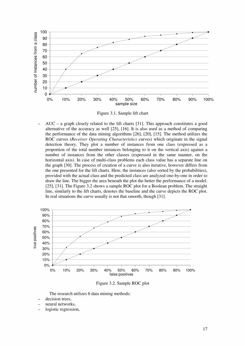
– AUC – a graph closely related to the lift charts [31]. This approach constitutes a goodalternative of the accuracy as well [25], [16]. It is also used as a method of comparingthe performance of the data mining algorithms [26], [20], [15]. The method utilizes theROC curves (Receiver Operating Characteristics curves) which originate in the signaldetection theory. They plot a number of instances from one class (expressed as aproportion of the total number instances belonging to it on the vertical axis) against anumber of instances from the other classes (expressed in the same manner, on thehorizontal axis). In case of multi-class problems each class value has a separate line onthe graph [30]. The process of creation of a curve is also iterative, however differs fromthe one presented for the lift charts. Here, the instances (also sorted by the probabilities),provided with the actual class and the predicted class are analyzed one-by-one in order todraw the line. The bigger the area beneath the plot the better the performance of a model.[25], [31]. The Figure 3.2 shows a sample ROC plot for a Boolean problem. The straightline, similarly to the lift charts, denotes the baseline and the curve depicts the ROC plot.In real situations the curve usually is not that smooth, though [31].

The research utilizes 6 data mining methods: – decision trees,– neural networks, – logistic regression,

Figure 3.1. Sample lift chart

0% 10% 20% 30% 40% 50% 60% 70% 80% 90% 100%

0

10

20

30

40

50

60

70

80

90

100

sample size

num

ber

of

insta

nces f

rom

a c

lass

Figure 3.2. Sample ROC plot

0% 10% 20% 30% 40% 50% 60% 70% 80% 90% 100%

0%

10%

20%

30%

40%

50%

60%

70%

80%

90%

100%

false positives

true p

ositiv

es

17

– clustering, – Naive Bayes, – association rules.

They have been all implemented in the business intelligence part of the Microsoft SQLServer 2005 [28] and this was the main reason for choosing them. The implementation isdescribed in the next chapter.

The following subsections describe the data mining methods in detail.

3.1 Decision Trees

Decision trees are one of the most popular data mining algorithms and knowledgerepresentation means [31]. They have been used in a variety of classification tasks, includingmedicine [23]. The process of building a tree is iterative and can be described in brief asfollows [31]: choose an attribute which goes to the root and then create a branch for each ofits values. These two steps are repeatedly performed until all of the attributes have beeninserted into the tree. This approach requires the attributes to take only discrete values.

Decision trees are very robust to noise in the data [23]. Trees classify future instancesby sorting them down the tree along branches that correspond to the values of the attributes.

The basic decision tree learning algorithm is called ID3. It has become outdated sinceits first publication in 1986 [23]. Nevertheless, it is important to understand the basics of ID3in order to be able to comprehend the modern approaches.

The ID3 algorithm builds a tree from the root down. The selection of the attributes togo to particular nodes is an integral part of the algorithm. Attributes that are the mostinformative (carry the most information which is determined by how well they alone classifyall the instances) are put closer to the root. The best one goes to the very root. This is agreedy search for a solution. A drawback of this algorithm is that it does not go back up thetree to review previous decisions about splits. This forms a bias which makes the algorithmfavor first acceptable solution over potentially better ones that may be out there in the spaceof possible solutions. Thus the tree may converge to a local minimum, not the global one.

The decisions about the splits are made basing on a statistical test called information

gain calculated for each attribute. As a measure ID3 uses entropy (equation (3.2)) whichdescribes the impurity of data.

Entropy S ≡∑i=1

c

�p i log2 pi(3.2)

where: S – collection of training instances, c – number of values of a class, pi – proportion of attributes with a class i in the entire set.

Then the information gain for each attribute is computed according to equation (3.3):

GainS , A≡Entropy S � ∑v∈Values A

∣Sv∣∣S∣

Entropy Sv (3.3)

where:Values(A) – a set of all possible values of an attribute ASv – a subset of S for which the attribute A take a value v.

The definition of the ID3 algorithm described above clearly states that attributes ofinstances have to take only discrete values. However there are ways of incorporatingcontinuous values as well. This process is called discretization and relies on splitting thecontinuous values into several subranges and treating them as discrete.

18

The ability of handling numeric values along with several other improvements, likeover-fitting avoidance technique and enhanced attribute selection measure [23] has beenintroduced in an ID3 successor, the C4.5 decision trees. The over-fitting avoidance aims atprotecting the tree from over training, i.e. adjusting the tree to much to the training datawhich may harm its predictive power on the future instances. The pruning method applied inthe C4.5 is the rule post-pruning. It transforms the tree into a set of rules and then removesparts of them that cause the over-fitting [23].

In the decision tree learning algorithms described above it was assumed that only oneattribute can be put in a node. Such trees are called univariate. On the contrary, there aremultivariate trees which allow for a number of attributes to decide about the split of a tree.Such approach has been introduced in Classification and Regression Trees (CART) [31]which are capable of creating linear combinations of attribute values in order to decide abouta split of the tree. Such trees are often more accurate and smaller in size in comparison withC4.5, but the process of learning takes much longer. Also their interpretation is moreproblematic. CART is capable of both regression and classification depending on a type of aclass (dependent variable) [4].

3.2 Association Rules

Association rules are another form of knowledge representation [31]. Theygeneralize classification rules in a way that they allow for predictions of any attribute values,not just a class. This also gives them the ability of predicting combinations of attributes.Also, unlike classification rules, the association rules are to be used individually, not as a set[31].

Association rules can be generated from even small datasets. Often the number of therules is very large, with most of them not containing any relevant knowledge. In order todetermine which rules potentially carry the most information two measures have beenintroduced [31]:– coverage – also referred to as support, denotes a number of instances a rule applies to,– accuracy – also referred to as confidence, expresses a number of instances correctly

predicted in proportion to all of the instances the rule applies to. Rules are similar to trees in terms of the type of the algorithm used to create them

[31]. Both trees and rules use divide-and-conquer type of algorithms which rely on splittingthe training set. However, there are differences in the representation: rules are easier tounderstand from a humans' perspective. An algorithm used in rules induction is calledcovering. Unlike the one used in ID3, it chooses attributes which maximize separationamong attributes, while in case of the trees it aims at maximization of the information gain.Also, in the association rules it is possible for a rule to have not only a set of attributes on theleft side, but also the right side can comprise any number of them (not only the class). Therule induction algorithm is run for every possible combination of attribute values on the leftand the right sides. This poses a serious computational problem and delivers an enormousnumber of rules. This approach is not efficient and often infeasible. Instead the algorithmseeks for the most frequent item sets (sets of attribute/value pairs) with support at somepredefined level. These item sets are then transformed into rules. This process consists oftwo stages:

1. generation of all the possible combinations of rules that can be derived from a givenitem set and calculating accuracy of each of these rules

2. removal of all of the rules whose accuracy is lower than a predefined value. This way the ultimate rule set contains only the best of them.

19

3.3 Clustering

Clustering, as mentioned before, is a common name for all the algorithms which aimat grouping examples based on some regularities or resemblance among them. There are twotypes of clustering [28]: – hard clustering in which an instance may belong to one cluster only,– soft clustering in which an instance may belong to several cluster with different

probabilities. One way of grouping the instances is based on their distance to the centers of

clusters. This algorithm is called k-means [28] and is a hard clustering technique of groupinginstances. The algorithm takes a parameter k which specifies a number of clusters to becreated. Initially the centers of the clusters are chosen randomly and all of the examples areassigned to the nearest one based on the Euclidean distance. The instances in each cluster arethen used to compute a “new” center (or a mean) of the cluster. The whole procedure startsover for the new centers and is repeated until the positions of clusters' centers remain thesame in two consecutive iterations. At this point the clusters are stabilized and will stay assuch forever. This does not mean that this is the only possible arrangement of groups,though. The division of instances obtained this way probably constitutes only a localminimum. The algorithm is very sensitive to the initial random choices of clusters' centers.Even slight difference in this choice may end up in the totally different grouping. Besidesthat, the k-means has some other drawbacks. There is a chance that it will fail to find optimalgrouping. As an example of such situation the author of [31] describes a rectangle with fourinstances located at its corners (Figure 3.3). Assuming that two natural clusters containinstances at the ends of the shorter sides (the gray dashed ellipses), let's imagine a situationwhen initial centers have been picked in the middles of the longer sides (the two graysquares). This creates a stable situation in which the clusters contain instances from the endsof the longer sides (the two solid-lined ellipses) because they are near the centers.

The k-means algorithm also, due to the fact that it adopts distance as a determiner ofbelonging of the instances to the clusters, is only applicable to data for which it is possible tocompute the distance (i.e. numeric). It seems senseless to calculate distance between colorsor diagnoses, for instance. This issue has been addressed in the EM algorithm.

The EM algorithm – expectation maximization [28] – unlike k-means, bases onprobability when assigning instances to clusters. Thus it represents soft clustering becauseindividual instances may belong to several groups at once. The method requires initiallyrandom Normal distributions with some means and standard deviations assigned to each ofthe clusters [23]. Afterwards, these distributions are used to initialize k clusters by guessingthe probabilities at which particular instances belong to each cluster. The algorithm then triesto converge to real distributions and probabilities. Unlike the k-means, in the EM stoppingcondition is not that easy to determine as the algorithm will never reach the ultimateoptimum. The process is iteratively repeated until convergence to a predefined, “good-enough” value.

Figure 3.3. A situation when the k-means algorithm does not deliver an optimal solution. Two graysquares denote the initial choice of the cluster centers, dashed ellipses show the natural clusters, the

solid-lined ones – the actual grouping.

20

3.4 Naive Bayes

The Naive Bayes is a quick method for creation of statistical predictive models [28].The algorithm, being a simple one, is used in a variety of other fields of science. The authorsof [31] even claim that Naive Bayes sometimes gives better results than other moresophisticated algorithms such as neural networks. They encourage researchers to try thisalgorithm first, before applying more difficult and complex solutions.

The naivety of the algorithm results from the fact that it assumes the variables(attributes) to be independent. This assumption, being not true in most real-life situations,usually delivers a model with a good predictive power [28]. The learning process relies oncounting correlations (combinations) of each of the values of each attribute with each valueof a class. The probability of an instance E consisting of attributes' values n1, n2,...,nk to beclassified as belonging to a class H is estimated with the use of the following equation (3.4):

Pr [E∣H ]≈N !⋅∏i=1

k P i

ni

ni !(3.4)

where N = n1, n2,...,nk and P i

ni denotes a probability of a particular value of an

attribute ni to be correlated with a class value H [31].

However, if only a single value of an attribute has not been associated with the valueof the class the entire equation evaluates to 0. This, in turn, means that the value of the classwill never be predicted for any of the instances. This drawback can be easily eliminated byassuming that all the correlations are possible. This can be done in a variety of ways. One ofthe most common is to use some coefficients incorporating external knowledge into themodel [28]. The assumption that all of the correlations are possible is such an externalknowledge. This approach can for instance increase all the numbers of correlations by 1which will eliminate the “0 correlations” allowing the model to predict any value of theclass.

3.5 Artificial Neural Networks

Artificial neural networks have been inspired by the human brain [23]. They are builtof neurons, which in this context are simply some computational units which combine inputs(with the use of the combination function) in order to produce an output (with the use of theactivation function). The networks are not sensitive to errors in the training data but requirelong time of learning [23]. They usually deliver predictions for future instances very fast,though. However, understanding of the prediction mechanism often poses serious troubles.

The neurons of a network are arranged in layers [23]. The first one is called an inputlayer and receives the values of the input attributes that are to be analyzed. It is followedby an optional set of hidden layers containing hidden neurons. They allow the network toperform nonlinear predictions [23]. The last layer is the output one which delivers theresults. A flow of data is conducted along connectors between the neurons. Each connectorhas a weight assigned. A network is nothing more than a graph with nodes (units) andinterconnections [28]. There are several types of networks: feed-forward and non-feed-forward. The former does not allow for cycles in the graph, while the latter does. Thisresearch is going to be focused only on feed-forward multi-layered networks.

It is usually not easy to determine the best topology of a neural network, i.e. thenumber of hidden neurons [28]. The more hidden neurons the longer training time andcomplexity of the network. Solutions to this problem vary and depend on implementationand problems to which a network is applied.

The aim of the learning process is to minimize the output error of predictionsexpressed as a squared error between the actual output and the target values [23]. This is

21

done by adjusting the weights assigned to each connector which are randomly guessedbefore the process starts. There are many algorithms for learning a neural network. One ofthe most popular is called back-propagation in which the error is calculated according to thefollowing equation (3.5):

E w≡12∑d ∈D

∑k∈outputs

t kd�okd (3.5)

where outputs denotes the set of output neurons of the network, tkd and okd are thetarget and output values respectively, associated with k-th output neuron and trainingexample d from the set D.

There are two approaches to adjustments of the weights [28]. The first is called thecase (or online) updating in which they are modified after each individual instance haspassed through the network. Alternatively, the error can also be back-propagated once afterthe entire training set has been pushed through the network. Such method is called the epoch

(or batch) updating. In order to understand the learning process the authors of [31] advise to imagine the

error as a surface in a 3-dimensional space. The aim is to find its minimum. The problem iswhen the surface has a number of them. The way the back-propagation algorithm works –stochastic, gradient descent – unfortunately does not guarantee that a global minimum willbe reached. Often the learning stops when the error descends to a local one. Nevertheless,the artificial neural networks are commonly used in medicine giving decent results [13],[12], [7].

3.6 Logistic regression

Logistic regression is a statistical algorithm which is applicable to dichotomyproblems [31]. It is a better alternative for a linear regression which assigns a linear model toeach of the class and predicts unseen instances basing on majority vote of the models. Suchapproach has a drawback because it does not deliver proper probability values as the outputvalues may fall outside the range [0,1]. The logistic regression, in turn, builds a linear modelbased on a transformed target variable whose values are not limited to only 0 or 1 but takeany real value instead [31]. The transformation function is called a logit transformation

presented in Figure 3.4. The resulting model is approximated by the equation (3.6):

Pr [1∣a1, a2,... , ak ]=1

1exp �w0�w1 a1�...�w k ak (3.6)

where wi denotes weights of particular attributes. The Figure 3.5 presents a samplelogistic regression function.

The weights in the regression function (equation (3.6)) are adjusted so that they fit thetraining data. The algorithm strives for maximizing the log-likelihood (equation (3.7)) as ameasure of this fitting [31].

∑i=1

n

1�xi log1�Pr [1∣a1

i, a2

i , ... , ak

i ]xi logPr [1∣a1

i , a2

i , ... , ak

i ] (3.7)

where x(i) equals either 0 or 1.

22

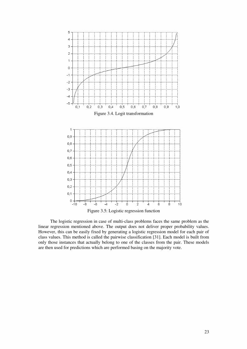
The logistic regression in case of multi-class problems faces the same problem as thelinear regression mentioned above. The output does not deliver proper probability values.However, this can be easily fixed by generating a logistic regression model for each pair ofclass values. This method is called the pairwise classification [31]. Each model is built fromonly those instances that actually belong to one of the classes from the pair. These modelsare then used for predictions which are performed basing on the majority vote.

Figure 3.4. Logit transformation

Figure 3.5: Logistic regression function

23

4 IMPLEMENTATION OF THE DATA MINING METHODS IN THE

MICROSOFT BI SQL SERVER 2005

In the previous chapter several data mining algorithms have been described. They allhave been well defined theoretically. However, various analytical systems implement themin a number of different ways. The actual performance strongly depends not only on the veryalgorithm, training data, or a computational power of a machine. It may also be affected byspecific features with which algorithms have been equipped by their implementers. Thedevelopers and system architects are free to introduce any constraints and alterations to theway an algorithm works and performs predictions. The aim of this research is to evaluate theimplementation of several algorithms in the business intelligence part of the Microsoft SQLServer 2005 [28].

The Microsoft SQL Server 2005 offers 9 algorithms to be chosen from: 1. Microsoft Association Rules2. Microsoft Decision Trees3. Microsoft Clustering4. Microsoft Time Series5. Microsoft Naive Bayes6. Microsoft Sequence Clustering7. Microsoft Neural Network8. Microsoft Linear Regression9. Microsoft Logistic Regression

In fact, the Microsoft SQL Server 2005 implements only seven of the above.The Microsoft Linear Regression is realized with use of the Microsoft Decision Treeswhich do not branch and the Microsoft Logistic Regression is realized with use of theMicrosoft Neural Network without hidden neurons.

In the research only the following algorithms have been evaluated: MicrosoftAssociation Rules, Microsoft Decision Trees, Microsoft Clustering, Microsoft Naive Bayes,Microsoft Neural Network and Microsoft Logistic Regression. The reason for rejecting thetime series and the sequence clustering is the fact that the analytical data used in the researchis not related to time. It does not contain any information about the sequence of events whichis necessary in order to apply these algorithms [28]. More detailed description of theanalytical data is provided in the Chapters 5 and 6. The reason for rejecting the linearregression, besides the one described in the previous chapter, is the non-linearity of the datafrom the surveys of the Breast Cancer Prevention Program.

Initial overview of the system allows for drawing a conclusion that Microsoft does notfollow commonly accepted trends in the data mining. As an example one can give a lack ofcross-validation during the construction of a model. Instead the Microsoft SQL Serverapplies some other measures which stop further development of a model when somecondition is met. A user cannot influence the training process by any means other thanthrough several parameters which vary among the algorithms. Results are presented in analgorithm-specific viewer which allows both to visualize the model along with some otherfeatures dependent on the algorithm. The Microsoft SQL Server implements only twoperformance measure techniques: a lift chart and a classification matrix [28]:– lift chart – as described in the Chapter 3 is a plot depicting a lift factor. In the Microsoft

SQL Server the concentration of a class (the vertical axis) in the sample is expressed as aratio of its concentration in the entire dataset (population). There are two modes in whichthe lift chart can be viewed. The first shows the correct classifications in the sampledataset (the accuracy). This mode is triggered when the user does not select any classvalue to plot. If the class value has been selected the proper lift chart is built. It containsat least three lines. One for the randomly guessed model, the second for the ideal modeland the third for the model that is being analyzed. In case when more models are

24

examined at the same time, each of them has its line on the chart. The Figure 4.1 shows asample lift chart created in the Microsoft SQL Server 2005.

– classification matrix – as described in the previous chapter.

The following subsections describe implementation of particular algorithms in theMicrosoft SQL Server 2005.

4.1 Microsoft Association Rules

The Microsoft Association Rules are based on the Apriori algorithm [28]. Asmentioned in the previous chapter association rules are the generalized version of theclassification rules in a way that they allow for prediction of any attribute. The MicrosoftAssociation Rules method does not generate rules with multiple attributes on the right side,though. However, it is possible to perform multi-attribute prediction via issuing a predictivequery to the entire model [28]. The method requires the input attributes to be discrete.

The algorithm seeks for the most frequent item sets of attributes' values in the trainingset. They are created in the first step of the learning process. The second stage is to transformthese sets into rules.

The method, besides the support and the confidence (described in the previouschapter), adds an extra feature which characterizes the rules: importance. It expressesdependencies among attributes in a rule or in an item set. If the importance equals 1 then twoattributes are independent. If the value is less then 1 the attributes are negatively correlated,which means that increased probability of occurrence of one attribute decreases theprobability of occurrence of the other one (negative correlation). In turn, values greater than1 denote positive correlation.

Generation of the item sets can deliver a large number of them. In order to keep onlythose that are relevant from the perspective of further analyses the Microsoft AssociationRules introduces a parameter MINIMUM_SUPPORT, which provides a minimal thresholdfor the value of the support. This and other parameters are presented in the Table 4.1.

The Microsoft Association Rules can be used to perform predictions. This is done intwo steps. First the model looks for the rules whose left sides match an instance to predict. Incase there are no such rules the method applies a marginal statistical test to deliver the mostmatching ones. The rules with the most probability are the ones that give the most accuratepredictions.

Figure 4.1. Sample lift chart generated by the Microsoft BI SQL Server 2005

25

Table 4.1. Parameters of the Microsoft Association Rules

Parameter Description

MINIMUM_SUPPORT Defines a minimum support for item sets and rules.

MAXIMUM_SUPPORT Defines a maximum support for item sets and rules.

MINIMUM_PROBABILITY Defines a minimum probability for an association rule.

MINIMUM_IMPORTANCE Defines a minimum importance of a rule.

MAXIMUM_ITEMSET_SIZE Defines a maximum size of an item set

MINIMUM_ITEMSET_SIZE Defines a minimum size of an item set.

MAXIMUM_ITEMSET_COUNT Defines a maximum number of item sets.

4.2 Microsoft Decision Trees

The Microsoft Decision Trees incorporate features of the C4.5 and the CARTalgorithms [28]. Thus they are capable of performing predictions both in discrete andcontinuous problems. A tree can be grown on training data which contains errors.

The Microsoft Decision Trees can handle multi-class problems. The default behaviorof the algorithm in case of a class with more than 100 values is that it takes 99 the mostpopular ones and one representing all of the other values. After each split this subset can bechanged, based on the class values' distribution.

The algorithm does not implement pruning. Instead, the growth of a tree is controlledin two ways:– Bayesian score – a score which stops further growth of a tree if the remaining data does

not justify any more splits,– parameter COMPLEXITY_PENALTY – a parameter which takes values from 0 to 1,

where the higher the value to smaller the tree. Another important parameter is the SCORE_METHOD which defines the score

method, i.e. the function applied to the attributes to calculate the best split of the tree. Thehigher the score the more chance for the tree to split on the given attribute. There are threefunctions available: entropy, Bayesian with K2 prior (BK2) and Bayesian DirichletEquivalent with Uniform prior (BDEU). The first has been described in the Chapter 3. Thesecond adds a constant value (prior) to the class value in each node of the tree regardless ofthe level in that tree [28]. The third, in turn, takes the level of a node into consideration whileadding a weighted value (prior) to the class values in the tree nodes [28]. In these twomethods the closer to the root the higher the prior. This prior also allows for incorporatingsome external knowledge into the tree [28]. The Table 4.2 presents the rest of theparameters.

The algorithm performs feature selection step before starting the training process [28].Too much attributes may result in a long learning time and large resources utilization.The Microsoft Decision Trees applies the feature selection not only to the attributes but also,in some cases, to the predictable variables (classes). This step is controlled by twoparameters: MAXIMUM_INPUT_PARAMETERS and MINIMUM_INPUT_PARAMETERS.This is the only way users may influence the feature selection process, which is invokedinternally beyond any user's attention.

The Microsoft Decision Trees can handle continuous inputs [28]. The discretizationdivides such attributes into a number of buckets (99 by default). The next step is to mergeneighboring ones, however only those pairs which can increase a split score of the tree. Thisstep is performed iteratively until any further merging is harmful to the tree's performance.

The output model of Microsoft Decision Trees algorithm may contain several trees(that is why the name of the algorithm is plural) [28]. This fact is used to perform association

26

analysis. The trees may be connected with each other showing interrelations between theirindividual nodes.

Table 4.2. Microsoft Decision Trees parameters

Parameter Description

COMPLEXITY_PENALTY Used to control the growth of a tree.

MINIMUM_SUPPORT Defines a minimum size of leaves in a tree.

SCORE_METHOD Defines a method to measure the split score atduring the training process.

SPLIT_METHOD Specifies a shape of a tree (binary, bushy).

MAXIMUM_INPUT_ATTRIBUTES Specifies a maximum number of attributes andinvokes feature selection when the number of inputparameters is greater than its value

MAXIMUM_OUTPUT_ATTRIBUTE

S

Specifies a maximum number of output attributes.

FORCE_REGRESSOR Specifies one of the attribute to be a regressor (usedin regression trees).

4.3 Microsoft Clustering

The Microsoft Clustering implements two clustering algorithms: k-means andexpectation-maximization (EM) [28]. They were described in the Chapter 3.

Despite the fact that the k-means is traditionally not applicable to discrete problemsthe Microsoft Clustering uses an alternative distance measure, which allows it to be used forsuch problems. The distance is calculated as one minus the probability that a particular valuebelongs to a cluster.

The Microsoft Clustering can be used to perform predictions on top of the grouping.The model can predict any of the missing attributes of an unseen instance. First, the model,basing on the known values of the attributes, looks for a cluster which the instance best fitsto. Next, based on the values in the cluster, the model reads the missing value and itsprobability (if that is the case).

During the analyses the user can see the profile of each of the clusters. Furthermore, itis possible to see what features distinguish each cluster from the others.

The Table 4.3 presents the parameters which control the behavior of the method.

Table 4.3. Microsoft Clustering parameters

Parameter Description

CLUSTERING_METHOD Species an algorithm used to determine clustermembership: Scalable EM, Non-scalable EM,Scalable K-Means, Non-scalable K-Means.

CLUSTER_COUNT Specifies how many clusters to find, 0 will force thealgorithm to guess the number of them based onheuristics.

MINIMUM_SUPPORT Defines a minimum number of instances belonging toa cluster

27

MODELING_CARDINALITY Defines a number of candidate models to createduring the training process

STOPPING_TOLERANCE Stopping condition of the training process, determinesthe maximum number of cases when an instancechanges membership.

SAMPLE_SIZE Defines a number of instances used to train the model,setting it to 0 will force the model to use all theavailable ones.

CLUSTER_SEED A random number used to initialize clusters.

MAXIMUM_INPUT_ATTRIBUTES Specifies a maximum number of input attributes. Ifthere are more attributes than this value, automaticfeature selection is triggered.

MAXIMUM_STATES Specifies a maximum number of states (values) of anattribute. If there are more states then only the mostpopular are used.

4.4 Microsoft Naive Bayes

The Microsoft Naive Bayes does not introduce any specific constraints other than forthe numbers of attributes [28]. These numbers are limited with the use of the model'sparameters presented in the Table 4.4. Also the method requires the input attributes to bediscrete.

The implementation uses the independent probability, the prior, to incorporateexternal knowledge and to eliminate the shortcoming of an algorithm described in theChapter 3.

Table 4.4. Microsoft Naive Bayes parameters

Parameter Description

MAXIMUM_INPUT_ATTRIBUTES Specifies a number of input parameters(255 by default)

MAXIMUM_OUTPUT_ATTRIBUTES Specifies a number of output parameters(255 by default)

MAXIMUM_STATES Specifies a number of states (values) ofattributes to consider during the trainingprocess

MINIUMUM_DEPENDENCY_PROBABILIT

Y

Specifies the dependency between an inputvariable and the class.

4.5 Microsoft Neural Network

The Microsoft Neural Network is an implementation of a feed-forward neural network[28] (no cycles in the graph are allowed). As mentioned in the Chapter 3 there are two typesof functions associated with each neuron: combination and activation. In the MicrosoftNeural Network as the combination function a weighted sum of inputs is used. Activationfunction, in turn, depends on whether a neuron is hidden or output. In case of the former,tanh (2) is used, while the latter has the sigmoid (3).

28

o=ea�e�a

eae

�a(2)

where o – output value, a – input value.

o=1

1ea (3)

where o – output value, a – input value.

The Microsoft Neural Network is trained according to the back-propagation

algorithm. A sum of squared deltas (differences) between the actual and the expected outputis used as an error function in case of continuous attributes. Otherwise, the algorithm usescross-entropy [28]. As far as the weights adjustment is considered the Microsoft NeuralNetwork utilizes epoch (or batch) updating approach described in the Chapter 3. Accordingto the authors of [28] this gives better results in regression problems.

The Microsoft Neural Network allows only for one hidden layer [28]. The number ofhidden neurons is determined by an equation (4):

c⋅n⋅m (4)

where: c denotes a constant dependent on a problem, in case of the Microsoft NeuralNetwork set to 4 by default, modifiable by the user. Variables n and m denote the number ofinput and output attributes respectively.

The Microsoft Neural Network also imposes constraints on the number of outputneurons (limited to 500). In case when there are more attributes, automatic feature selectionalgorithm is triggered. The network is not visualized in the system in any way.

The Table 4.5 presents model's parameters.

Table 4.5. Microsoft Neural Network

Parameter Description

MAXIMUM_INPUT_ATTRIBUTES Specifies a maximum number of input attributes.

MAXIMUM_OUTPUT_ATTRIBUTE

S

Specifies a maximum number of output attributes.

MAXIMUM_STATES Specifies a maximum number of states (values) anattribute can take

HOLDOUT_PERCENTAGE Specifies a percentage of training data that is heldout for validating purposes.

HOLDOUT SEED Specifies a seed for selecting a holdout set.

HIDDEN_NODE_RATIO Specifies a value of c variable in the (4) equation.Default value is 4.

SAMPLE_SIZE Specifies a size of the data used for training.

29

4.6 Microsoft Logistic Regression

The Microsoft Logistic Regression constitutes a totally different approach from thecanonical algorithm described in the Chapter 3. It is based on the Microsoft Neural Network.

The logistic regression implemented in the SQL Server 2005 does not calculate linearmodels for class values but uses the Microsoft Neural Network without a hidden layer tocreate them, instead. Such network, with the use of the sigmoid function, generates the sameregression models as the logistic regression algorithm itself. The only reason that the modelis available for users is its discoverability. Thus the model has the same parameters, althoughthe Hidden_Node_Ratio is set to 0 and not modifiable.

30

5 SOURCES OF THE ANALYTICAL DATA

The analyses performed within this research are based on the data from the PolishNational Breast Cancer Prevention Program. The following subsections provide detaileddescription of the Program as well as the data reception process.

5.1 Polish National Breast Cancer Prevention Program

The Polish National Breast Cancer Prevention Program was held under the dispositionof the President of the Polish National Health Fund [2] in 2006. The reason for startingthe Program, as described in the Chapter 1, was the fact that the breast cancer is the mostfrequent malignant cancer in Polish women. It constitutes about 20% of all the malignantcancers. Its occurrence probability increases after menopause or after 50 years of age.According to the Polish Central Statistical Office (Polish: Główny Urząd Statystyczny, GUS)almost 11 000 women went down with the disease in 2000. The number of cases increasedfrom 50,5 in 1999 to 55,3 in 2000 per 100 000 women. Observations have proved thatsudden increase in the occurrence of the cancer takes place in women between 50 and 69years of age. Forecasts for the future are pessimistic. It has been estimated that each year theoccurrence rate increases by 0,7% [2]. This allows for drawing a conclusion that actionstaken to detect and identify breast tumors in an early stage are still insufficient.

Oncologists and physicians are still not certain what is the cause of the cancer. This isdespite huge amount of work and analyses dedicated to the disease by doctors aroundthe world. This research is particularly difficult because the same type of breast cancer canbe induced by several factors (carcinogens) [2]. Scientists indicate that genetic heritage playsa significant role. In Poland about 10% of breast cancer cases are in women who have beendiagnosed to have mutations in the BRCA1 gene. However, genes are only oneof the possible carcinogens. These are the others:

– age between 50 and 69– breast cancer in family, especially in close relatives (mother, sister), – said mutations within genes– early menstruation (before 14 years of age),– late menopause (after 55 years of age),– birth after 35 years of age,– lack of children,– previous breast cancer related treatment,– treatment due to some other breast illnesses.Scientists agree that the most crucial factor deciding about success or failure of the

treatment is the early detection. A method which allows for discovery of any disorders in abreast tissue is the mammography. Its sensitivity reaches about 90-95% for women aftermenopause. Random screenings reduced the death rate by 25-30% in women who had theirmammography each year or two [2]. American College of Preventive Medicine recommendsmammography in 2 projections, every second year to women between 50 and 69 years of agewho belong to a so-called “low-risk” group, and every year to women from “high-risk”group.

The importance of the health problem is really high. In populations where there is noscreenings held whatsoever, there is high mortality rate due to the invasive breast cancer [2].This cancer, besides social price, requires a very costly treatment. Depending on howadvanced the tumor is the treatment may require operation (amputation), radiotherapy orsystem treatment (chemotherapy, hormonal therapy). All these means are very costly. Theoverall cost consists of cost of an operation and therapies, cost of treatment of complications,expenses resulting from disability pensions, sick-leaves, social care and so forth.

31

Another problem constitute psychological and social effects resulting from the illness or adeath in family.

A lot has already been done in order to increase the level of knowledge concerningthe breast cancer. From 1976 to 1990 Polish government ran the National Tumor FightingProgram. Within this Program screenings in some areas of Poland were introduced whichaimed at early detection of the breast cancer. This allowed for creation of a model of a breastcancer screening program and its implementation in the six leading centers in Poland.

Similar research has been held all over the world [2]. In the USA and the EuropeanUnion it has been agreed that the most effective means of fighting malignant cancers arenational cancer prevention programs. Such programs are financed by the governments.Activities within such a program should include, besides the screenings, also purchase ofmodern equipment for diagnosis and treatment and education of the society and the medicalestablishment. Experiences learned by western countries, which has been running suchprograms for a long time now, indicate that they are effective and really reduce mortality rateeven by 33% in women before 50 years of age.

Objectives of the Polish Program included the reduction of a death rate in Polishwomen due to the breast cancer and also a decrease of that rate to the level present in themodern European countries. Also the founders of the Program hoped to increase the level ofknowledge concerning the disease and its prophylaxis. Another objective was to increase therate of early detection which guarantees better treatment results.

The Program targeted women between 50 and 69 years of age who had not had amammography within last 24 months. Women, who had had a breast cancer alreadydiagnosed, were not eligible for the Program.

The Program consisted of two parts: basic and extended. Within the former a patientwas asked to fill out a survey stating her current health condition and other important aspectsof her life. This part constituted the appendix 1. Afterwards she underwent a mammographyscreening which, along with the description and the Mammography Card created by aradiologist (the appendix 2), were kept on her file. Basing on the results of the screening thepatient was referred (appendix 3) to further screening (extended) if it was considerednecessary. Otherwise the patient's attendance in the Program ended. Within the extended partof the screening the patient underwent some additional examinations. These includedphysical screening, additional mammography or ultrasonography (USG), fine needleaspiration or core needle biopsy [2]. The results were documented in the Extended ScreeningCard (the appendix 4). All the actions and a flow of control have been depicted in the Figure5.1.

The data comes from the surveys from a Clinical Hospital No. 1 in Wrocław.

32

5.2 Data reception

The National Breast Cancer Prevention Program was based on surveys filled outby patients and cards filled out by doctors. The Program required medical staff to store thedata in paper and parts in digital documents (only parts filled out by the doctors). Thereception process consisted of three stages:

1. development of a software tool enabling convenient data input to the database,2. manual data input (using the tool) from the patients' parts of the surveys,3. automatic data input from the digital documents.

The software tool (of a working name DataRetriever), developed for the purposeof the data input, provides several features. It is a user oriented application which allowsfor creation of a number of users that can belong to one of three groups: administrators,doctors and administrative staff. Each role gives them special permissions, for instance: theadministrative staff cannot input other data than personal information of the patients,administrators, in turn, have a right to manage users and perform some additionaladministrative operations like batch input.

The main window of the tool closely reflects the way the surveys are organized. Thismeans that the arrangement of particular fields in the survey has been mirrored in theapplication. This makes the data input convenient.

The tool was developed in the .NET Framework 2.0 and requires such to run. Thesystem uses the Microsoft SQL Server 2005 database management system.

33

6 ANALYTICAL DATA PREPARATION

The research is based on a data warehouse into which the data is loaded. Thefollowing subsections provide a brief introduction to data warehousing and describe thedesign of the warehouse used in the research followed by the ETL process.

6.1 Introduction to data warehouse modeling

Han and Kamber in [14] define a data warehouse as “semantically consistent data storethat serves as a physical implementation for a decision support data model and stores theinformation on which an enterprise needs to make strategic decisions”. Often the datawarehouse systems are referred to as OLAP (On-Line Analytical Processing) systems whichdiffer from the operational ones (OLTP – On-Line Transactional Processing) by theirpurpose. The OLAP ones are used to support decisions by querying large amounts ofaggregated data whereas the OLTP serve as a means for managing data in everyday work[14]. There are several terms essential to understanding the data warehousing process:– dimension – a perspective from which the data can be viewed. They may be hierarchical

(e.g. year – quarter – month – day). Their purpose is to describe the measures (facts),– fact – a numerical measure represented in a fact table along with dimensions. Often it is

not easy to determine what data should be put as a fact. Kimball and Ross [18] give anadvice that facts should be additive along each of the dimensions. This means that itshould be possible to sum the values of the fact along each and every dimension. Forinstance quantity of sales are additive along such dimensions as time, product, storebecause one can add up the sales value per year, per product or per store. But, forinstance bank account balance is not additive along the time dimension because onecannot sum the values as it would give senseless results.

A data warehouse stores and presents the data in a multidimensional manner [18].These dimensions along with facts form data cubes – a basic object in a data warehousewhich stores the data in an aggregated form.

Before creation of the data cubes a data warehouse schema has to be designed. Suchdesign takes a form of a relational database in which the unified data is gathered andaggregated. There are two basic forms of the design of the data warehouse schema [18]:– star schema – this paradigm allows for a large fact table surrounded by smaller,

denormalized dimension tables, – snowflake (constellation) schema – this paradigm allows for normalization of the

dimension tables. This means that they can keep their data in some additional tablesassociated with them.

There are a number of ways of modeling a data warehouse. Han and Kamber [14]describe four views that have to be considered while designing a data warehouse. – top-down view – selection of the most important information that the data warehouse

will model,– data source view – relates to the operational data sources which contain data that is

going to be loaded into the data warehouse,– data warehouse view – relates to fact tables and dimensions,– business-query view – a view from the perspective of an end-user.

The first view has been done by analyzing the surveys in order to the parts that carriedrelevant information. These are described later in this chapter. The second view required theexamination of the operational database – the one the DataRetriever tool worked on. Thethird view was done according to a methodology proposed by Todman [29]. This approachdivides the data warehouse schema design into three stages: conceptual, logical and physical.Todman proposed a convenient way of designing the conceptual model – dot modeling. Inhis approach a fact is modeled as a dot surrounded by dimensions. Such model, if properly

34

created, shows all the relationships among facts and dimensions, for instance it is easilypossible to determine shared dimensions (i.e. those that are used by several data cubes). It isalso easy to see what schema model (star or snowflake) suits better the data. The last view(the business-query view) is beyond the scope of this research.

Han and Kamber [14] prove that a data warehouse can be used for knowledgediscovery with the use of data mining methods as one of three applications of datawarehouses. Besides the data mining, warehouses can be used in information processing(basic statistical analyses) and analytical processing (advanced operations). The differencebetween the analytical processing and the data mining comes from the fact that processingperforms aggregations and summarizations of the data while data mining automatically seeksfor implicit patterns allowing for prediction, clustering and association. OLAP with datamining is called On-Line Analytical Mining (OLAM). There are several reasons for whichOLAM is beneficial from the business perspective [14]:– data warehouse usually contains high quality data – this fact may have a significant

impact on the quality of the data mining models,– availability of information processing tools that are usually incorporated into data

warehouse environments – these include database access providers, integration,consolidation and transformation of heterogeneous data sources (even remote),

– it provides means for analyses conducted on portions of data at various granularities,drilling the data through to see which records influenced particular decisions,

– integration of OLAP functions into data mining allows the users to dynamically swapdata mining algorithms.

A very important step on the way to a data warehouse is the ETL process [19].The abbreviation stands for: Extraction, Transformation and Loading. The first partof the process embraces all the actions that are required to extract the data from various,often heterogeneous operational data sources. This also includes pre-cleaning. The secondstep encompasses all the transformations that the data has to go through in order to fitthe data warehouse model. In this phase data is aggregated, cleaned and transformed so thatit could be loaded into a data warehouse. The very loading is performed in the last stage.Here also some additional cleaning is possible.

The next subsections describe the design of the data warehouse schema used in thisresearch as well as the ETL process performed during data preparation.

6.2 Medical data warehouse model

The design of the data warehouse utilized in the research followed the three models(conceptual, logical and physical) design pattern described by Todman [29]. In theconceptual phase dot modeling was employed. During this stage dimensions as well as factswere identified. The second stage was the transformation of the conceptual model into thelogical one. The transformation included supplementing the dimensions with their attributes.The last stage performed a further transformation into the physical model. It added variousplatform specific features to the model, such as primary and reference keys to the fact anddimension tables.

CONCEPTUAL MODEL

Figure 6.1 presents the conceptual model of the data warehouse. During this stage 9dimensions were identified. The granularity of the model was set at a particular location ofthe cancer, i.e. a specific place (behind nipple, centrally or in the so-called Spence's tail) inone of the breasts. This is the reason for creation of the following dimensions (they werebased on the information contained in the surveys):– FamilyDisease – represents the occurrences of breast cancer in a family of a patient.

It is important to distinguish close (first line) and distant (second line) just as it was in

35

the surveys. In case of the first line relatives it should also be noted what age the cancerwas diagnosed: before or after 50 years of age.

– TimeMonth – time dimension, generated on the basis of the dates of mammographies,concerns only 2006.

– Patient – represents patients taking part in the screening.– TissueType – a type of breast tissue: fat, fat-glandular, glandular-fat, glandular.– Symptom – represents symptoms discovered by the patients in their breasts.– BIRADS – represents BIRADS marks – used in oncology to denote the level of intensity

of a change in the breast tissue, takes integer values from the range [2;5] with 2 being theleast intensive and 5 being the most intensive change.

– Diagnosis – represents a diagnosis of a particular breast cancer case.– ScreeningResult – represents a result of the screening.– ChangeLocation – represents a location of a change in a breast: behind nipple, centrally

or in the so-called Spence's tail.

LOGICAL MODEL

The next step in the data warehouse modeling process is the logical model. During thisphase dimensions' attributes are identified. The model has been presented in the Figure 6.2.The dimensions identified in the conceptual model have been supplied with their attributes(also based on the surveys):– FamilyDisease

– FamilyLine – denotes the family line of a relative, this attributes also encodes theage in case of close relatives,

– Relative – denotes the relative (e.g. sister, mother, aunt, grandmother, etc.).– TimeMonth

– Month – denotes a month in the time dimension; this concerns only months in 2006.– Patient

– Age – age of the patient,– Births – a number of births (1 or more). This attribute also encodes the age of a first

delivery (before of after 35 years of age),– City – city of the patient's residence,– FirstMenstruation – age at first menstruation,– HormonalTherapiesEarlier – Boolean value indicating whether the patient applied

any hormonal therapies earlier in her life,– HormonalTherapiesNow – Boolean value indicating whether the patient applied any

hormonal therapies at the time of the screening,– LastMenstruation – denotes the age at the last menstruation, – MammographiesCount – denotes the total number of mammographies the patient

had in her life,

Figure 6.1. Data warehouse conceptual model

36

– ScreeningNumber – denotes a number of the screening, assigned by the medical staffupon performing the screening,

– SelfExamination – Boolean value indicating whether the patient self-checks herbreasts.

– TissueType

– TissueTypeName – a name of a type of a tissue.– Symptom

– SymptomDescription – description of a symptom.– BIRADS

– BIRADSDescription – denotes a change (such as architecture disorder, tumor,calcification, etc.),

– BIRADSValue – denotes a value of the mark from the range [2;5] which expressesthe intensity of the change.

– Diagnosis

– DiagnosisDescription – the description of a diagnosis, takes one of the followingvalues: norm, mild, probably mild, suspicious and malignant.

– ScreeningResult

– ChangeCount – number of changes discovered in a location,– ChangeSide – side (either left or right) of the change,– ChangeSize – size of the change expressed in millimeters.

– ChangeLocation

– ChangeLocation – location of the change, takes on of the following values: behindnipple, centrally, in the so-called Spence's tail.

In this stage usually a fact is also identified. However, the data that comes from thesurveys does not contain any numeric value that could be used as a fact. Potentially, adiagnosis could be a good candidate for a fact, but it would violate the additivity requirementdescribed in the previous subsection. However, there is a possibility to add a fully additivefact to the data warehouse that is being designed. This is a so-called calculated measure [28]which is computed after deployment of a data cube. In this case such fact would the numberof cases. It obviously is additive along each of the 9 identified dimensions.

PHYSICAL MODEL

Physical model is the last step of modeling a data warehouse. It transforms the logicalmodel so that it fits a dedicated, concrete database management system. In this phasereference constraints are added to the tables which entails addition of keys. The resulting

Figure 6.2. Data warehouse logical model

37

model can be implemented. The Figure 6.3 presents the physical view of the data warehousein the target environment which is the Microsoft SQL Server 2005.

The Microsoft SQL Server 2005 allows for mining data aggregated in a datawarehouse [28]. The way it is done is similar as if the analyses were performed on aregular data table. Furthermore, in the latter case also a virtual data warehouse cubeis created. The results of the analyses are equal in both cases. The reason for creatinga warehouse is the fact that it requires the data to be cleansed prior to loading. It is adesired process especially in case of such dirty data as used in the research.

6.3 ETL process

The data warehouse schema created and implemented in the previous step has to benow fed with the data. However, before this can happen the data has to be prepared. Thepreparation includes (but is not limited to) the following activities:– data transformation so that it fits the data warehouse schema– data cleansing so that only complete and unified data gets loaded into the warehouse.

In order to perform the ETL process the Microsoft Integration Services environmenthas been used. The Figure 6.4 shows the steps of the data integration process conducted onthe oncological data gathered from the surveys of the Program. The individual componentsrepresent the following activities:– Create database schema – this task reads an external SQL script and runs it against the

Microsoft SQL Server 2005 to create the data warehouse schema.– Symptoms preparation – this data flow task creates the dimension of symptoms. Here the

symptoms are aggregated and unified. For instance several patients stated that they feltpain in many different ways. This is to unify the descriptions of the symptoms.

– TissueType preparation – this task aggregates the possible types of a breast tissue andalso translates the names into English. Here the cleaning was not needed because thesurvey did not allow for putting own descriptions.

– Diagnosis preparation – this task creates the Diagnosis dimension. It aggregates thepossible diagnoses and inserts them into the dimension table.

– TimeMonth preparation – this task creates the time dimension based on themammographies dates of the surveys. All the dates are from 2006.

Figure 6.3. Data warehouse physical model

38

– BIRADS preparation – prepares the BIRADS dimension. This task cleanses andaggregates the BIRADS marks due to the fact that the surveys allowed the patients toenter their own descriptions which vary significantly. It also translates the names intoEnglish.

– FamilyDisease preparation – this task creates the FamilyDisease dimension. It performsthe encoding of the possible values stored in the data warehouse. These values includeage of a relative in whom cancer was diagnosed and the family line (either first orsecond).

– ChangeLocation preparation – this task prepares the ChangeLocation dimension. Itdiffers from the rest in a way that it does not retrieve any data from the operationaldatabase. The dimension's possible values have been hard-coded into the componentbecause they are fixed.

– ScreeningResult preparation – this task creates the dimension of screening results. Itaggregates the related data from the operational database.

– Patients preparation – this task prepares the dimension of the patients. The data iscleansed by removing patients with missing values.

– Fact preparation – this is the most complex task. Basing on the values of the incomingrecords it looks up values in the dimension tables seeking for matching data. In this taskalso the granularity is set. The incoming records are at the higher granularity (patientlevel) while the data warehouse expects it to be at the change location level.

– Check Database Integrity Task – the final task which is responsible for checking the datawarehouse for data integrity. This includes for instance conformance to referenceconstraints.

As a result of the ETL process 1311 breast cancer facts have been added to the datawarehouse.

6.4 Quality issues

Quality of the data is a very important aspect in the data mining. It has a superiorsignificance while building a data warehouse or data mining models [14]. Even though someof the algorithms are resistant to noise in the data, it is obvious that training processgenerates better results when the data is clean.

Figure 6.4: Data integration project in the Microsoft Integration Services environment for the datafrom the Breast Cancer Prevention Program (the ETL process)

39

The analytical data from the surveys of the National Breast Cancer PreventionProgram also required cleaning. The surveys were filled out by patients who, from variousreasons, tend to provide false or incomplete information. This was probably due to eitherpersonal issues or mistakes in the surveys' design. Passing over the personal reasons themistakes could result from rather poor organization of the questions in the survey. Thisconcerns locations of the questions on the form. Some of them could be easily overlookedbecause they were placed for instance in the upper right-hand corner. Furthermore, a lot ofanswers depended on answers to other questions. For instance checking the age of a firstbirth required to specify the number of birth greater than 0. For some reason some patientfailed to mark all the information. Errors also were frequent in the parts filled out by doctors.They were supposed to enter information regarding the screening into the survey. However,very often all they did was to attach a free text note stating the results of the screening,leaving the survey blank. Such free text notes are very difficult to analyze.

Due to the reasons stated above many of the surveys had to be excluded during thevery reception process. In other cases attempts were made to recover the values based on thecontext. Ultimately, the training data set contained only 1311 cases from approximately8000.

40

7 DATA ANALYSES

The training dataset, obtained from the surveys of the National Breast CancerPrevention Program, was used to build several data mining models. They included: decisiontrees, clusters, neural networks, logistic regressions, association rules and Naive Bayes.However, prior to this the dataset has been pre-analyzed. This was to see how the attributesare represented in terms of their values to determine the initial input set of attributes. Thiswas followed by the analyses.

The following subsections describe pre-analyses followed by the initial featureselection and the description of the experiment. Finally, the description of particular datamining models is provided which is concluded with an evaluation of all of them.

7.1 Data pre-analyses

Before building the data mining models the dataset has been pre-analyzed to see howeach attribute is represented. This step allows to see diversity of values of each attribute andtheir distribution. This fact is a good basis for delivering conclusions concerning whether thedataset contains enough data for the models to learn. It will also enable for initial featureselection. Attributes poorly represented are not informative enough to be taken into accountduring the learning process.

The first dimension of the data warehouse is the Patient. The nine subsequent chartsplot the particular patients' attributes' values against the number of instances carrying them.Figure 7.1 shows the distribution of the Age attribute. Even though the Program wasdedicated to women between 50 and 69 years of age, nine women from beyond this rangealso had the screening done. The most numerous group comprises women aged between 51and 59 (at least 80). The least representative groups contain women younger than 50 or olderthan 60 (less than 35).

Figure 7.1. Distribution of the Age attribute

1

45

98 96

133

144138

85 83 84

117

63

14

33 31

17

30

1423

3226

4

0

20

40

60

80

100

120

140

160

45 50 51 52 53 54 55 56 57 58 59 60 61 62 63 64 65 66 67 68 69 70

41

The next attribute is the Births. As mentioned in the Chapter 6 it encodes the numberof births along with the age at which the patient had the first delivery. Figure 7.2 presents thedistribution of values of this attribute. It shows that the most women had at least 2 childrenand their first delivery was before they turned 35 (700 cases). A significant proportion ofwomen did not have any children (249 cases) or had only one at a young age (330 cases).The chart plots a tendency of women having their first children before 35 years of age or nothaving children at all.

The Program was dedicated to women from the Lower Silesia province in Poland. TheFigure 7.3 presents the cities which the attendees were from. The number of them was toolarge to display all of them on one graph. For the simplicity's sake the cities, which appear inthe data less than 10 times have been grouped under the common label Other. The traditionalcapital city of the province – Wrocław – is the most frequent in the data.

Figure 7.2. Distribution of the Births attribute.

249

330

25

700

7

0

100

200

300

400

500

600

700

800

No children 1 child before 35

years of age

1 child after 35

years of age

2 and more

children (1st one

before 35 years of

age)

2 and more

children (1st one

after 35 years of

age)

Figure 7.3. Distribution of the City attribute.

14 12 12 18 16 24 12

958

16

229

0

200

400

600

800

1000

1200

DzierŜ

oniów

Jelcz

Las

kowice

Konin

Lubań

Łany

Św. K

atar

zyna

Trze

bnica

Wro

cław

Zako

pane

Other

42

The surveys contained questions concerning various facts from patients' lives. Thesefacts can have a significant impact on the final class of an instance. The Figures 7.4 and 7.5present the distribution of the age at which the patients had their first and last menstruationrespectively. In case of the former the dominant value is 14 (447 instances). In turn, the lastmenstruation was the most frequent between the ages 48 and 52 (at least 100 instances). Thevalue 100 on the latter graph represents the patients that still have the menstruation.

Another very important aspect of a patient's life is whether they took any hormonaltherapies. Figures 7.6 and 7.7 show the distributions of the therapies taken earlier and atpresent. Most of the patients declare that they have never taken hormonal therapies, neither

Figure 7.4. Distribution of the FirstMenstruation attribute.

2 1 1

60

203

287

447

172

91

27 20

0

50

100

150

200

250

300

350

400

450

500

8 9 10 11 12 13 14 15 16 17 18

Figure 7.5. Distribution of the LastMenstruation attribute

23 31 32 35 37 38 39 40 41 42 43 44 45 46 47 48 49 50 51 52 53 54 55 56 57 58 59100

0

25

50

75

100

125

150

175

200

225

250

1 3 1 2 1 4 2 3 1

28

54

24

66

3125

106101

243

130

191

9488

56

196 7 2

22

43

before nor now. The proportion of those that admit applying such therapies at present ismuch lower than the same indicator in the past.

The vast majority of the patients had had mammography screenings prior to signing upfor the Program. Most of them, however, did not have more than 5 such screenings (at least100 of patients per a number of mammographies). Only few patients had more than 10mammographies. Figure 7.8 presents the distribution of this attribute.

Figure 7.7. Distribution of the HormonalTherapiesNow attribute

1208

103

0

200

400

600

800

1000

1200

1400

False True

Figure 7.6. Distribution of the HormonalTherapiesEarlier attribute.

842

469

0

100

200

300

400

500

600

700

800

900

False True

44

In Poland the breast cancer awareness have been increased by several previous actions,either local or nationwide [2]. This resulted in the patients paying attention to their health bydoing occasional self-examinations. This fact is presented in the Figure 7.9:

In the surveys, the patients also had to provide descriptions of symptoms that theyobserved during such self-examinations (the Symptom dimension of the data warehouse).The survey had a few options but also provided some space to add extra ones. The Figure

Figure 7.8. Distribution of the MammographiesCount attribute

179

259274

198

158

122

65

10 5 10 17 122

0

50

100

150

200

250

300

0 1 2 3 4 5 6 7 8 9 10 12 15

Figure 7.9. Distribution of the SelfExamination attribute

1

1310

0

200

400

600

800

1000

1200

1400

False True

45

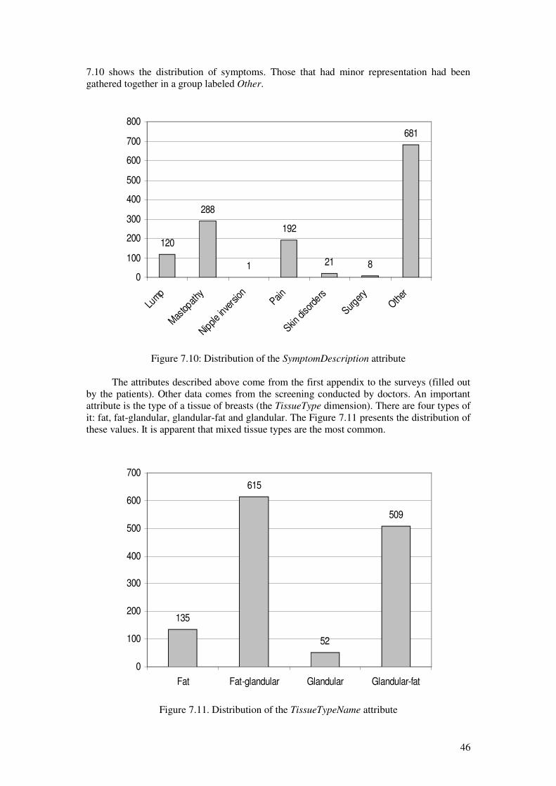
7.10 shows the distribution of symptoms. Those that had minor representation had beengathered together in a group labeled Other.

The attributes described above come from the first appendix to the surveys (filled outby the patients). Other data comes from the screening conducted by doctors. An importantattribute is the type of a tissue of breasts (the TissueType dimension). There are four types ofit: fat, fat-glandular, glandular-fat and glandular. The Figure 7.11 presents the distribution ofthese values. It is apparent that mixed tissue types are the most common.

Figure 7.11. Distribution of the TissueTypeName attribute

135

615

52

509

0

100

200

300

400

500

600

700

Fat Fat-glandular Glandular Glandular-fat

Figure 7.10: Distribution of the SymptomDescription attribute

120

288

1

192

21 8

681

0

100

200

300

400

500

600

700

800

Lump

Mas

topat

hy

Nipple

inve

rsion Pain

Skin d

isord

ers

Surger

yOth

er

46

Besides the tissue type the doctors also identified and measured the changes within thebreasts. The measurements were expressed with the use of the BIRADS marks (the BIRADS

dimension) described previously in the Chapter 6. There are three potential changes inbreasts identified by the doctors: architecture disorders, calcification and lump. Theirdistribution has been presented in the Figure 7.12. The most common are the architecturedisorders.

The Figure 7.13, in turn, shows the distribution of the BIRADS values. The mostcommon value is 2, which denotes a minor change in terms of its intensity and size.However, a significant proportion constitutes the value 3. Value 5 – the most intensivechange – did not appear in the dataset.

Figure 7.12: Distribution of the BIRADSDescription attribute

878

147

286

0

100

200

300

400

500

600

700

800

900

1000

Architecture disorders Calcification Lump

Figure 7.13: Distribution of the BIRADSValue attribute

843

449

19 00

100

200

300

400

500

600

700

800

900

2 3 4 5

47

Besides the BIRADS marks, the changes are also described with use of the followingmetrics: a number of them (Figure 7.14), side (left or right, Figure 7.15) and size (Figure7.16) from the ScreeningResult dimension and location (behind nipple, centrally or in the so-called Spence's tail, Figure 7.17) from the ChangeLocation dimension. Their distributionshave been presented in the four subsequent figures (Figures 7.14, 7.15, 7.16 and 7.17).

Figure 7.14. Distribution of the ChangeCount attribute

301

947

4418 1

0

100

200

300

400

500

600

700

800

900

1000

0 1 2 3 5

Figure 7.15. Distribution of the ChangeSide attribute

667

644

630

635

640

645

650

655

660

665

670

Left Right

48

As indicated in the Chapter 5 the breast cancer's occurrence strongly depends onwhether this disease was diagnosed in the family or not. The Figure 7.18 shows thedistribution of this attribute in the dataset. The most common value is None, which denotesthe fact that the disease did not appear in the family. The second most frequent value is theFirst_After50 which denotes the diseases in the first-line family members (mother or sister)

Figure 7.16: Distribution of the ChangeSize attribute

1013

4 35 61 57 30 14 858

7 1 4 11 2 3 30

200

400

600

800

1000

1200

0 3 4 5 6 7 8 9 10 12 13 15 20 25 30 40

Figure 7.17. Distribution of the ChangeLocation attribute

301

478

405

127

0

100

200

300

400

500

600

BehindNipple Central None SpenceTail

49

in whom the disease was discovered. The disease in the second-line members is also veryfrequent.

The following figure (Figure 7.19) presents the distribution of the occurrence of thedisease with respect to the relatives. Similarly to the Figure 7.18 the value None is the mostfrequent (the values are equal which is logical, because these two attributes are dependent).However, the most common relatives that went down with the disease are the first-linemembers of the family (mother being the most frequent and sister being the second).

Figure 7.18: Distribution of the FamilyLine attribute

9553 76

1087

0

200

400

600

800

1000

1200

First_After50 First_Before50 Second None

Figure 7.19. Distribution of the Relative attribute

9157 56

20

1087

0

200

400

600

800

1000

1200

Mother Sister Aunt Grandmother None

50

The last attribute – the time (in months) – is presented in the Figure 7.20. The monthsin which the physicians conducted the most screenings are: February, October andNovember. This attribute does not carry any relevant information from the perspective of thepredictions, because it encompasses a short period of time (1 year). It has been put here forstatistical purposes only.

Finally, the Figure 7.21 presents the distribution of the class (DiagnosisDescription). Itis apparent that the instances are far from being equally distributed among the class values.The Malignant class is very poorly represented (only 3 cases). This fact can have asignificant impact on the data mining models and analyses because too few training instancesfrom a particular class do not give enough information to train the model.

Figure 7.21. Distribution of the DiagnosisDescription attribute, which is theclass for the instances

640

469

104 95

30

100

200

300

400

500

600

700

Norm Mild ProbablyMild Suspicious Malignant

Figure 7.20. Distribution of the Month attribute

16

200

8674

122

90

5668

99

192 188

120

0

50

100

150

200

250

Janu

ary

Febr

uary

Mar

chApr

ilM

ayJu

neJu

ly

Augus

t

Septe

mbe

r

Octob

er

Novem

ber

Decem

ber

51

7.2 Initial feature selection

The analytical dataset comprises several attributes. However, some of them do notcarry any relevant information from the perspective of the analyses. For instance, theScreeningNumber in no way can influence the occurrence of the breast cancer. In case of theCity one can argue that some cities are more polluted than others and living there mayinfluence the disease. However, in case of this research the patients come from a small areain Poland (one province) and all of the cases are close-to-equally affected in this regard.Thus this attribute will also be skipped. The Table 7.1 shows the attributes both that havebeen chosen for the analyses and those that have been rejected.

Table 7.1. Initial feature selection

Attribute Accepted Reason for rejection

FamilyDisease dimension

FamilyLine Yes

Relative No This attribute is dependent on the FamilyLine.

Time dimension

Month No Time span within which the Program was conductedis too short and in no way influences the occurrenceof the disease.

Patient dimension

Age Yes

Births Yes

City Yes

FirstMenstruation Yes

HormonalTherapiesEarli

er

Yes

HormonalTherapiesNow Yes

LastMenstruation Yes

MammographiesCount No Numbers of mammographies taken by a patient doesnot affect the disease.

ScreeningNumber No It is only a statistical attribute introduced foradministrative purposes and carries no medicalinformation.

SelfExamination No It is uninformative because only one case (out of1311) bears a different value from all the rest. It mayadd a lot of noise to the data.

TissueType dimension

TissueTypeName Yes

Symptom dimension

SymptomDescription Yes

BIRADS dimension

BIRADSDescription Yes

BIRADSValue Yes

52

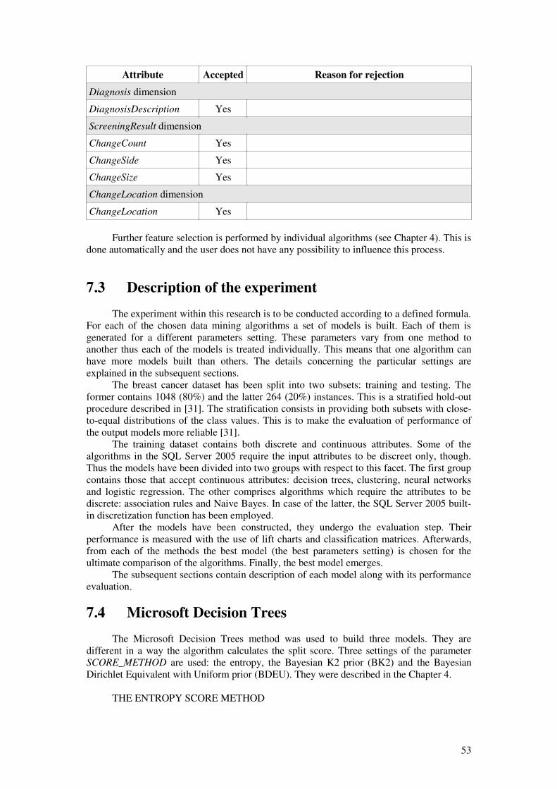
Attribute Accepted Reason for rejection

Diagnosis dimension

DiagnosisDescription Yes

ScreeningResult dimension

ChangeCount Yes

ChangeSide Yes

ChangeSize Yes

ChangeLocation dimension

ChangeLocation Yes

Further feature selection is performed by individual algorithms (see Chapter 4). This isdone automatically and the user does not have any possibility to influence this process.

7.3 Description of the experiment

The experiment within this research is to be conducted according to a defined formula.For each of the chosen data mining algorithms a set of models is built. Each of them isgenerated for a different parameters setting. These parameters vary from one method toanother thus each of the models is treated individually. This means that one algorithm canhave more models built than others. The details concerning the particular settings areexplained in the subsequent sections.

The breast cancer dataset has been split into two subsets: training and testing. Theformer contains 1048 (80%) and the latter 264 (20%) instances. This is a stratified hold-outprocedure described in [31]. The stratification consists in providing both subsets with close-to-equal distributions of the class values. This is to make the evaluation of performance ofthe output models more reliable [31].

The training dataset contains both discrete and continuous attributes. Some of thealgorithms in the SQL Server 2005 require the input attributes to be discreet only, though.Thus the models have been divided into two groups with respect to this facet. The first groupcontains those that accept continuous attributes: decision trees, clustering, neural networksand logistic regression. The other comprises algorithms which require the attributes to bediscrete: association rules and Naive Bayes. In case of the latter, the SQL Server 2005 built-in discretization function has been employed.

After the models have been constructed, they undergo the evaluation step. Theirperformance is measured with the use of lift charts and classification matrices. Afterwards,from each of the methods the best model (the best parameters setting) is chosen for theultimate comparison of the algorithms. Finally, the best model emerges.

The subsequent sections contain description of each model along with its performanceevaluation.

7.4 Microsoft Decision Trees

The Microsoft Decision Trees method was used to build three models. They aredifferent in a way the algorithm calculates the split score. Three settings of the parameterSCORE_METHOD are used: the entropy, the Bayesian K2 prior (BK2) and the BayesianDirichlet Equivalent with Uniform prior (BDEU). They were described in the Chapter 4.

THE ENTROPY SCORE METHOD

53

The Figure 7.22 shows a decision tree built with the use of the entropy as a scoremethod. The tree is very complex and contains 60 leaves.

Figure 7.22. Decision tree built with the use of the entropy score method

54

The classification matrix for the entropy decision tree is presented in the Table 7.2.The Malignant case has been mispredicted as Mild. The reason for this is probably the poorrepresentation of this value. A very interesting observation is the fact that the class values:Mild and Norm have high rates of misclassifications favoring one another. Also theProbablyMild value has been mispredicted in favor of the Norm and the Mild. TheSuspicious also has a high rate of misclassified instances in favor of the Norm class.

Table 7.2. Classification matrix of the decision tree with the entropy score method

Predicted Malignant

(Actual)

Suspicious

(Actual)

ProbablyMild

(Actual)

Mild

(Actual)

Norm

(Actual)

Malignant 0 0 0 0 0

Suspicious 0 1 0 1 0

ProbablyMild

0 0 0 0 6

Mild 1 0 16 14 12

Norm 0 18 5 79 110

THE BAYESIAN WITH K2 PRIOR SCORE METHOD

The Figure 7.23 shows a decision tree built with the use of the Bayesian with K2 prior(BK2). Unlike the one built with the entropy score method, the BK2 tree is much simpler; itcontains only 4 leaves.

The classification matrix for the BK2 tree is presented in the Table 7.3. In this casealso the Malignant cases have been misclassified, this time as the Norm class. All of theSuspicious instances have also been misclassified in favor of either Mild or Norm. Also all ofthe ProbablyMild instances were misclassified (as Norm). Poor results also gave the Mild

value. A great proportion of these instances have been classified wrongly as belonging to theNorm class. Excellent results were gained for the Norm value: all of these instances werepredicted correctly.

Table 7.3. Classification matrix for the BK2 tree

Predicted Malignant

(Actual)

Suspicious

(Actual)

ProbablyMild

(Actual)

Mild

(Actual)

Norm

(Actual)

Malignant 0 0 0 0 0

Suspicious 0 0 0 0 0

ProbablyMild

0 0 0 0 0

Mild 0 7 0 6 0

Norm 1 12 21 88 128

Figure 7.23. Decision tree built with the use of the Bayesian with K2 prior (BK2)

55

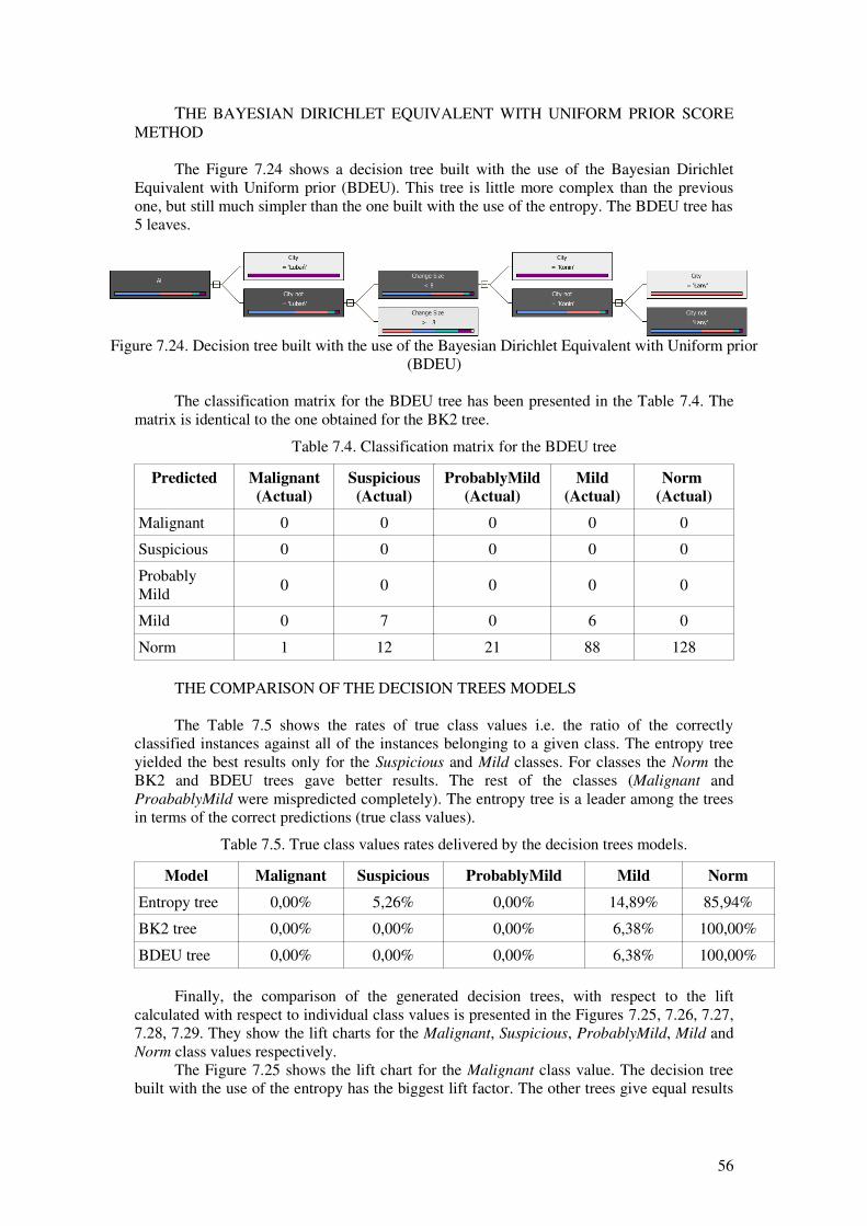
THE BAYESIAN DIRICHLET EQUIVALENT WITH UNIFORM PRIOR SCOREMETHOD

The Figure 7.24 shows a decision tree built with the use of the Bayesian DirichletEquivalent with Uniform prior (BDEU). This tree is little more complex than the previousone, but still much simpler than the one built with the use of the entropy. The BDEU tree has5 leaves.

The classification matrix for the BDEU tree has been presented in the Table 7.4. Thematrix is identical to the one obtained for the BK2 tree.

Table 7.4. Classification matrix for the BDEU tree

Predicted Malignant

(Actual)

Suspicious

(Actual)

ProbablyMild

(Actual)

Mild

(Actual)

Norm

(Actual)

Malignant 0 0 0 0 0

Suspicious 0 0 0 0 0

ProbablyMild

0 0 0 0 0

Mild 0 7 0 6 0

Norm 1 12 21 88 128

THE COMPARISON OF THE DECISION TREES MODELS

The Table 7.5 shows the rates of true class values i.e. the ratio of the correctlyclassified instances against all of the instances belonging to a given class. The entropy treeyielded the best results only for the Suspicious and Mild classes. For classes the Norm theBK2 and BDEU trees gave better results. The rest of the classes (Malignant andProabablyMild were mispredicted completely). The entropy tree is a leader among the treesin terms of the correct predictions (true class values).

Table 7.5. True class values rates delivered by the decision trees models.

Model Malignant Suspicious ProbablyMild Mild Norm

Entropy tree 0,00% 5,26% 0,00% 14,89% 85,94%

BK2 tree 0,00% 0,00% 0,00% 6,38% 100,00%

BDEU tree 0,00% 0,00% 0,00% 6,38% 100,00%

Finally, the comparison of the generated decision trees, with respect to the liftcalculated with respect to individual class values is presented in the Figures 7.25, 7.26, 7.27,7.28, 7.29. They show the lift charts for the Malignant, Suspicious, ProbablyMild, Mild andNorm class values respectively.

The Figure 7.25 shows the lift chart for the Malignant class value. The decision treebuilt with the use of the entropy has the biggest lift factor. The other trees give equal results

Figure 7.24. Decision tree built with the use of the Bayesian Dirichlet Equivalent with Uniform prior(BDEU)

56

which are below the plot of the random guesser. This fact makes the entropy tree the bestclassifier among the trees.

The Figure 7.26 presents the lift chart for the Suspicious class value. In this case theBayesian trees (BK2 and DBEU, equal results) give better lift factor in comparison with theentropy tree whose plot falls below the random guesser.

The Figure 7.27 depicts the lift chart for the ProbablyMild class value. The entropytree gives the best lift factor in comparison to the other trees.

Figure 7.25. Lift chart for the Malignant class for the decision trees

Figure 7.26. Lift chart for the Suspicious class for the decision trees

57

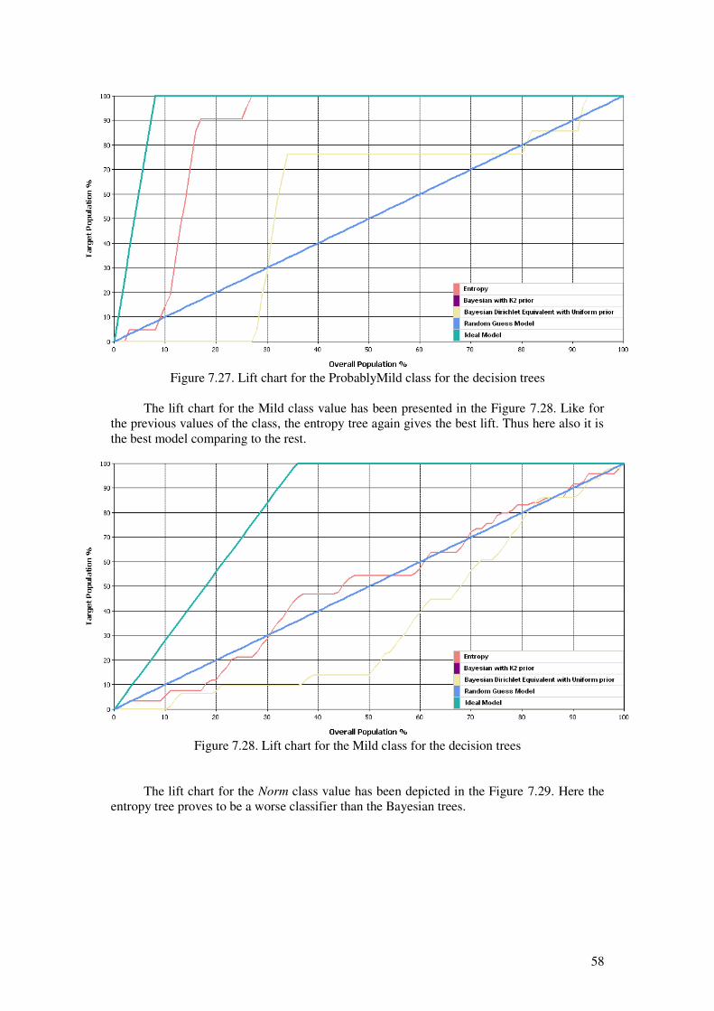
The lift chart for the Mild class value has been presented in the Figure 7.28. Like forthe previous values of the class, the entropy tree again gives the best lift. Thus here also it isthe best model comparing to the rest.

The lift chart for the Norm class value has been depicted in the Figure 7.29. Here theentropy tree proves to be a worse classifier than the Bayesian trees.

Figure 7.27. Lift chart for the ProbablyMild class for the decision trees

Figure 7.28. Lift chart for the Mild class for the decision trees

58

The lift charts for the decision trees, with respect to each of the class values show thatthe best lift factor in most of the cases (3 out of 5) was achieved by the tree built with the useof the entropy. The other score methods delivered models that are equal to each other interms of the lift factor. The classification matrices, in turn, showed that the BDEU and BK2score methods favor the majority class (the Norm value). The other class values predictionswere either the best in case of the entropy tree or equal to 0 for all of the trees. Thus theoverall best classifier was gained with the use of the entropy score method.

7.5 Microsoft Clustering

The Microsoft Clustering allows for building the model with two methods: the EM andk-means algorithms. This is done by setting the CLUSTERING_METHOD parameteraccordingly. The clusters have been built with the use of both of these algorithms. Thenumber of clusters has been set to the default value (10).

THE EM ALGORITHM

The Figure 7.30 shows the clusters generated with the use of the EM algorithm and therelationships among them. The darker the cluster the more instances it contains. Theassociations among the clusters are organized in the same manner, i.e. the darker the line themore similar the two clusters are.

Figure 7.29: Lift chart for the Norm class for the decision trees

59

The Figure7.31 shows the distribution of the class values in each of the clusters. Thecluster 10 contains the most instances from the Norm class. The ones which contain the leastof such instances are the clusters 4 and 8. The most Malignant cases contains the cluster 6.The rest of the class values are irregularly distributed among the clusters.

The classification matrix for the clusters generated with the use of the EM algorithm ispresented in the Table 7.6. Similarly to the decision trees the Malignant class wasmisclassified in all of its instances. The predictions favor the Norm class value. Very badresults were obtained for the Suspicious class – all of the suspicious instances weremisclassified either as Mild or Norm. The ProbablyMild class also delivered poor results asall of its instances were predicted as Norm. Poor results also gave the Mild class in case ofwhich most of the predictions were in favor of the Norm class. The very Norm class,however, gave excellent results (all correct classifications).

Figure 7.30. Clusters generated with the use of the EM algorithm

Figure 7.31. Distribution of class values in individual EM clusters

60

Cluster 1 Cluster 2 Cluster 3 Cluster 4 Cluster 5 Cluster 6 Cluster 7 Cluster 8 Cluster 9 Cluster 10

0,000

0,100

0,200

0,300

0,400

0,500

0,600

0,700

0,800

0,900

1,000

Malignant Suspicious ProbablyMild Mild Norm

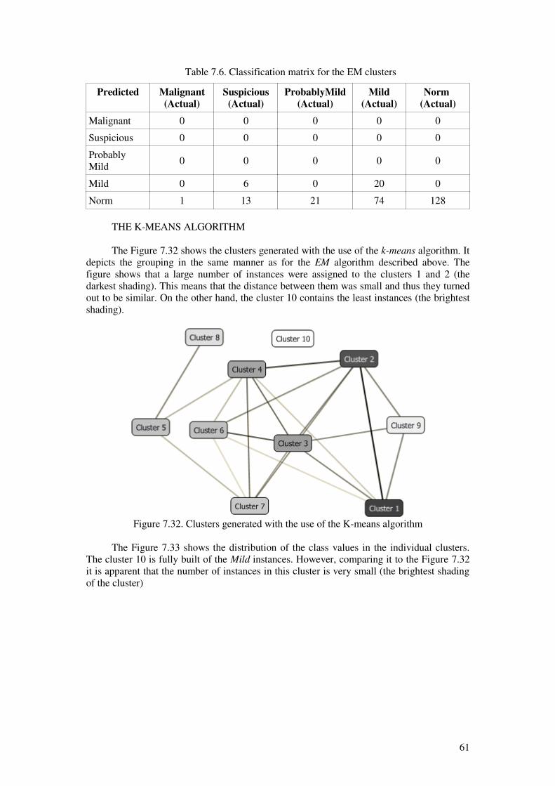
Table 7.6. Classification matrix for the EM clusters

Predicted Malignant

(Actual)

Suspicious

(Actual)

ProbablyMild

(Actual)

Mild

(Actual)

Norm

(Actual)

Malignant 0 0 0 0 0

Suspicious 0 0 0 0 0

ProbablyMild

0 0 0 0 0

Mild 0 6 0 20 0

Norm 1 13 21 74 128

THE K-MEANS ALGORITHM

The Figure 7.32 shows the clusters generated with the use of the k-means algorithm. Itdepicts the grouping in the same manner as for the EM algorithm described above. Thefigure shows that a large number of instances were assigned to the clusters 1 and 2 (thedarkest shading). This means that the distance between them was small and thus they turnedout to be similar. On the other hand, the cluster 10 contains the least instances (the brightestshading).

The Figure 7.33 shows the distribution of the class values in the individual clusters.The cluster 10 is fully built of the Mild instances. However, comparing it to the Figure 7.32it is apparent that the number of instances in this cluster is very small (the brightest shadingof the cluster)

Figure 7.32. Clusters generated with the use of the K-means algorithm

61

The classification matrix for the clusters generated with the use of the k-means

algorithms is presented in the Table 7.7. In this case also all of the Malignant instances havebeen misclassified. The predictions favored the Norm class. Similarly to the EM algorithm,here also the Suspicious class gave very bad results as all of the instances were wronglypredicted as belonging to either the ProbablyMild or the Norm classes. The ProbablyMild

class value delivered poor results too. All of the instances from this class were predictedeither as the Mild or the Norm. The Mild class was predicted wrongly as the Norm morefrequently than it was classified correctly. Again the best results were obtained for the Norm

class.

Table 7.7. Classification matrix for the k-means clustering

Predicted Malignant

(Actual)

Suspicious

(Actual)

ProbablyMild

(Actual)

Mild

(Actual)

Norm

(Actual)

Malignant 0 0 0 0 0

Suspicious 0 0 0 0 0

ProbablyMild

0 6 0 1 0

Mild 0 0 18 36 30

Norm 1 13 3 57 98

THE COMPARISON OF THE CLUSTERING MODELS

The Table 7.8 shows the rate of true class values delivered by the clustering models.The EM clustering model yielded slightly better results in terms of the true class values rate.The k-means was only little better in case of the Norm class. Very bad results were obtainedfor the Malignant and Suspicious class values.

Figure 7.33. Distribution of the class values in individual k-means clusters

62

Cluster 1 Cluster 2 Cluster 3 Cluster 4 Cluster 5 Cluster 6 Cluster 7 Cluster 8 Cluster 9 Cluster 10

0,000

0,100

0,200

0,300

0,400

0,500

0,600

0,700

0,800

0,900

1,000

Malignant Suspicious ProbablyMild Mild Norm

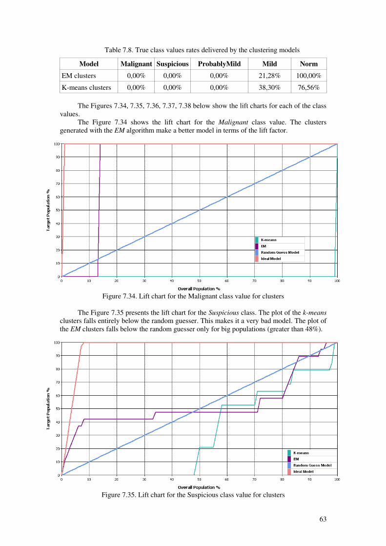
Table 7.8. True class values rates delivered by the clustering models

Model Malignant Suspicious ProbablyMild Mild Norm

EM clusters 0,00% 0,00% 0,00% 21,28% 100,00%

K-means clusters 0,00% 0,00% 0,00% 38,30% 76,56%

The Figures 7.34, 7.35, 7.36, 7.37, 7.38 below show the lift charts for each of the classvalues.

The Figure 7.34 shows the lift chart for the Malignant class value. The clustersgenerated with the EM algorithm make a better model in terms of the lift factor.

The Figure 7.35 presents the lift chart for the Suspicious class. The plot of the k-means

clusters falls entirely below the random guesser. This makes it a very bad model. The plot ofthe EM clusters falls below the random guesser only for big populations (greater than 48%).

Figure 7.34. Lift chart for the Malignant class value for clusters

Figure 7.35. Lift chart for the Suspicious class value for clusters

63

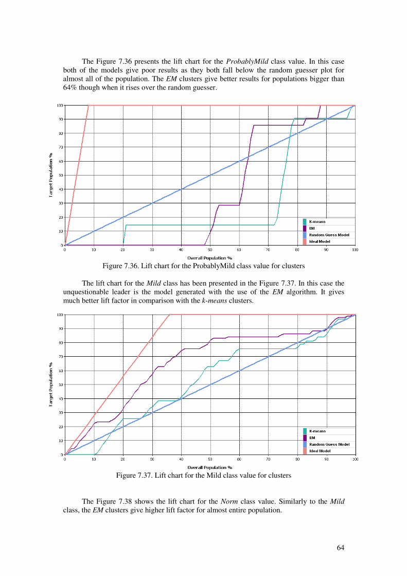
The Figure 7.36 presents the lift chart for the ProbablyMild class value. In this caseboth of the models give poor results as they both fall below the random guesser plot foralmost all of the population. The EM clusters give better results for populations bigger than64% though when it rises over the random guesser.

The lift chart for the Mild class has been presented in the Figure 7.37. In this case theunquestionable leader is the model generated with the use of the EM algorithm. It givesmuch better lift factor in comparison with the k-means clusters.

The Figure 7.38 shows the lift chart for the Norm class value. Similarly to the Mild

class, the EM clusters give higher lift factor for almost entire population.

Figure 7.36. Lift chart for the ProbablyMild class value for clusters

Figure 7.37. Lift chart for the Mild class value for clusters

64

The EM algorithm delivered a better lift factor for all of the class values. Onlysometimes, for some populations the k-means was favored. However, on in case of some ofthe classes both plots fell below the plot of the random guesser. This means that in practice itis more beneficial too choose the samples randomly than to use to model to select them.Nevertheless, in general the best lift factor has been gained with the use of the EMalgorithm.

7.6 Microsoft Neural Network

Since the Microsoft SQL Server 2005 does not implement the cross-validation theonly method available for testing the model is the holdout procedure [31]. This procedure isused during the creation of a network for validation purposes (to test the output error whileadjusting the weights). It is separate from the testing of a model which is done afterwardswith the use of the separate testing set. One of the parameters of the Microsoft NeuralNetwork allows for modifying the percentage of the instances that are used for testing theoutput error: the HOLDOUT_PERCENTAGE. For the purpose of this research two settingsare used. One is the default value: 30% of the instances used for testing. The second one hasbeen set to 60%. Even though a general truth says that the more instances used for thetraining the better the model, its quality also depends on the output error [31]. The authors ofthe [31] say that there has to be a trade-off introduced between the amount of instances usedfor training and those used for testing. They say that in order to obtain a good classifier asmuch of the instances as possible have to be used for training. On the other hand, in order toobtain a good error estimate as much of the instances as possible have to be used for testing.The experiment is to show how the split of the dataset influences the output model. The twonumbers: 30% and 60% are to demonstrate whether the quality of the output model is moredependent on the size of the training set or the testing set. In other words, this is to showwhether the model gives better results if more instances are used for training or for testingthe output error of a network. Two models are built for these two hold-out sets.

THE 30% HOLD-OUT SET

The Table 7.9 shows the classification matrix for the neural network built with the30% hold-out set. Similarly to the previous models, the Malignant class has been

Figure 7.38. Lift chart for the Norm class value for clusters

65

mispredicted in all of its cases. Unlike the previous models, the Suspicious class value gavebetter results. Nevertheless, majority of classifications were wrong. Bad results weredelivered for the ProbablyMild class value. The predictions mostly favored either the Mild orthe Norm values. In case of the Mild class, incorrect predictions outnumber the correct ones.The best results were gained for the Norm class.

Table 7.9. Classification matrix for the 30% split neural network

Predicted Malignant

(Actual)

Suspicious

(Actual)

ProbablyMild

(Actual)

Mild

(Actual)

Norm

(Actual)

Malignant 0 0 0 0 0

Suspicious 0 2 0 3 0

ProbablyMild

0 3 0 0 0

Mild 0 0 9 35 35

Norm 1 14 12 56 93

THE 60% HOLD-OUT SET

The Table 7.10 presents the classification matrix for the neural network built with the60% hold-out set. The results are very similar to what the 30% split delivered. This means inparticular poor results for the Malignant, the Suspicious and the ProbablyMild class values.The Mild value in this case has slightly worse results as the error is bigger. Again the Norm

class has the best outcome, however, much worse than in the previous case.

Table 7.10. Classification matrix for the 60% split neural network

Predicted Malignant

(Actual)

Suspicious

(Actual)

ProbablyMild

(Actual)

Mild

(Actual)

Norm

(Actual)

Malignant 0 0 0 0 0

Suspicious 0 0 0 0 1

ProbablyMild

0 2 0 0 0

Mild 0 4 15 25 52

Norm 1 13 6 69 75

THE COMPARISON OF THE NEURAL NETWORK MODELS

The Table 7.11 shows the rate of the correctly classified instances from a given classto the number of instances from this class. The results differ. The biggest difference is in thecase of the Suspicious class in the favor of the 30% split model, because the rate for the 60%split equals 0%. The other values are either equal to 0% or favor the 30% split model as well.

Table 7.11. True class values rates delivered by the neural networks models

Model Malignant Suspicious ProbablyMild Mild Norm

30% split 0,00% 10,53% 0,00% 37,23% 72,66%

60% split 0,00% 0,00% 0,00% 26,60% 58,59%

66

The Figures 7.39, 7.40, 7.41, 7.42 and 7.43 present the lift charts for each of the classvalues.

The Figure 7.39 presents the lift chart for the Malignant class value. The better liftfactor has been given by the model with 60% split of the dataset.

The lift factor for the Suspicious class has been presented in the Figure 7.40. In thiscase the 30% split of the dataset proves to be better for most of the population.

The Figure 7.41 depicts the lift chart for the ProbablyMild class value. The situationhere is different to the one presented for the Suspicious class (Figure 7.40). This means thatthe model with the 60% split of the dataset gives a better lift factor for most of thepopulations.

Figure 7.39. Lift chart for the Malignant class value for neural networks

Figure 7.40. Lift chart for the Suspicious class value for neural networks

67

The Figure 7.42 shows the lift chart for the Mild class value. In this case the plotclearly favors the model built with the use of the 30% split of the dataset. It gives a higherlift factor. The lift for the model built with the 60% split falls below the plot of the randomguesser regardless of the size of the population.

The Figure 7.43 shows the lift chart for the Norm class value. It also demonstrates thatthe 30% split gives a better lift. However, in this case the difference between the 30% andthe 60% split of the dataset is smaller than in case of the Mild class. The lift plot for the 60%is very close to the plot of the random guesser.

Figure 7.41. Lift chart for the ProbablyMild class value for neural networks

Figure 7.42. Lift chart for the Mild class value for neural networks

68

On most of the lift charts (3 out of 5) generated for the neural networks the one withthe 30% split of the dataset has a better lift factor. The Malignant class value, however,favors the 60% split. This may result from the poor representation of this class, though. Alsothe ProbablyMild class favors this split. In case of the rest of the class values the 30% modelis better because it has a better lift almost regardless of the size of the population.Nevertheless, the difference between the two models was small. This and the fact that notalways one model was better than the other allow for drawing a conclusion that the split ofthe dataset does not necessarily have a large impact on the output model (at least in case ofthe given dataset). Even though the latter case (the 60% split) used less than a half of theinstances for training it still delivered better results for the Malignant and ProbablyMild

class values. However, this may also be an effect of poor representation of the class values inthe set. This confirms the hypothesis that both the training set and the testing set are veryimportant in the learning process. The quality of the model (its predictive power) stronglydepends on both the training and the testing sets. However, it may turn out to be difficult todetermine the best split. It is then advisable to try out several combinations.

The results gained by the lift charts are confirmed by the true class values rates (Table7.11). The higher lift factor of the 60% split model in case of the Malignant and theProbablyMild classes cannot be credible because the true class value rate for these twovalues were equal 0%. Thus all of the instances from these classes were misclassified. Thepreferable neural network model is the one built with the use of the 30% split of the dataset.

7.7 Microsoft Logistic Regression

As mentioned in the Chapter 4, the Microsoft Logistic Regression is realized with theuse of the Microsoft Neural Network without the hidden layer. The analyses with the use ofthis method have been conducted in the same manner as for the neural networks describedabove. The reason for choosing the 30% and the 60% splits was the same as for the neuralnetworks.

THE 30% HOLD-OUT SET

The Table 7.12 presents the classification matrix for the logistic regression with the30% split of the dataset. Again the Malignant class value was misclassified in all of the

Figure 7.43. Lift chart for the Norm class value for neural networks

69

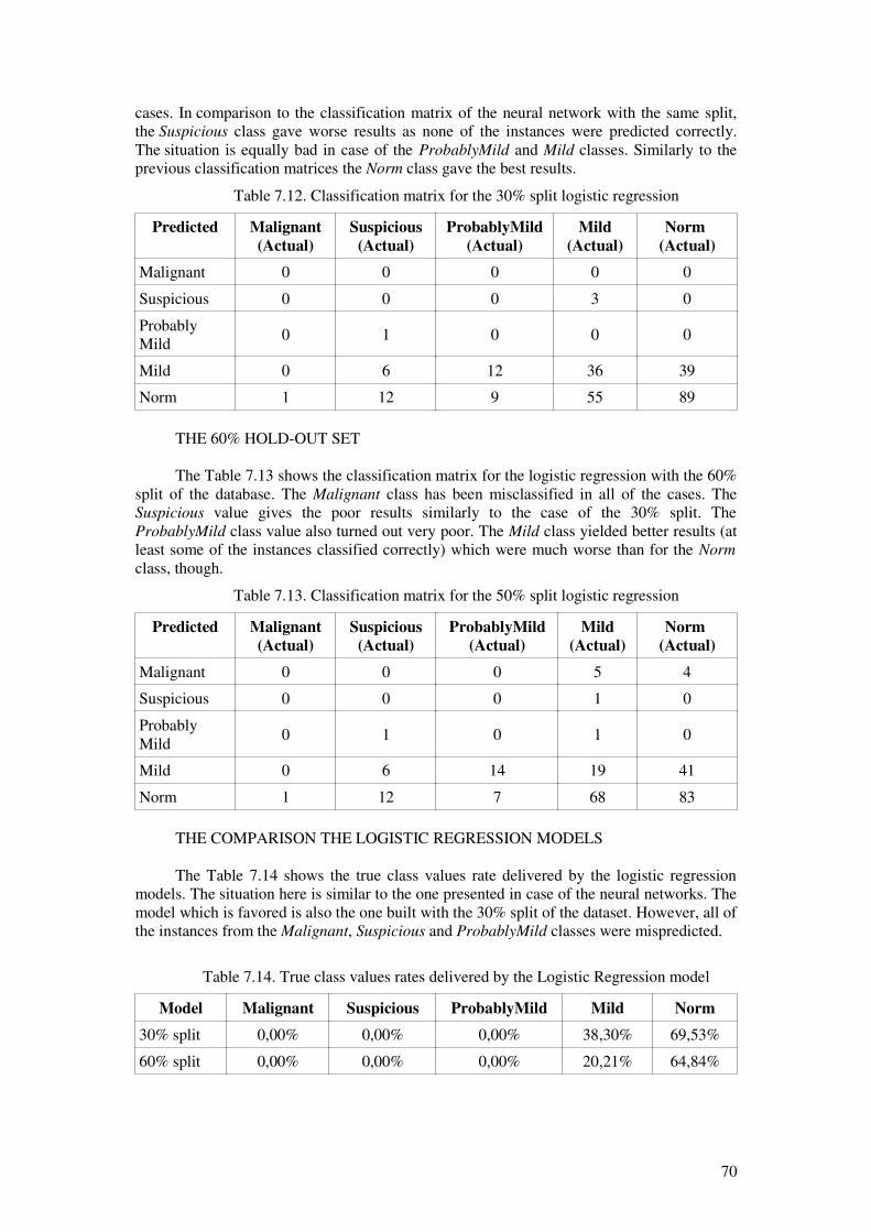
cases. In comparison to the classification matrix of the neural network with the same split,the Suspicious class gave worse results as none of the instances were predicted correctly.The situation is equally bad in case of the ProbablyMild and Mild classes. Similarly to theprevious classification matrices the Norm class gave the best results.

Table 7.12. Classification matrix for the 30% split logistic regression

Predicted Malignant

(Actual)

Suspicious

(Actual)

ProbablyMild

(Actual)

Mild

(Actual)

Norm

(Actual)

Malignant 0 0 0 0 0

Suspicious 0 0 0 3 0

ProbablyMild

0 1 0 0 0

Mild 0 6 12 36 39

Norm 1 12 9 55 89

THE 60% HOLD-OUT SET

The Table 7.13 shows the classification matrix for the logistic regression with the 60%split of the database. The Malignant class has been misclassified in all of the cases. TheSuspicious value gives the poor results similarly to the case of the 30% split. TheProbablyMild class value also turned out very poor. The Mild class yielded better results (atleast some of the instances classified correctly) which were much worse than for the Norm

class, though.

Table 7.13. Classification matrix for the 50% split logistic regression

Predicted Malignant

(Actual)

Suspicious

(Actual)

ProbablyMild

(Actual)

Mild

(Actual)

Norm

(Actual)

Malignant 0 0 0 5 4

Suspicious 0 0 0 1 0

ProbablyMild

0 1 0 1 0

Mild 0 6 14 19 41

Norm 1 12 7 68 83

THE COMPARISON THE LOGISTIC REGRESSION MODELS

The Table 7.14 shows the true class values rate delivered by the logistic regressionmodels. The situation here is similar to the one presented in case of the neural networks. Themodel which is favored is also the one built with the 30% split of the dataset. However, all ofthe instances from the Malignant, Suspicious and ProbablyMild classes were mispredicted.

Table 7.14. True class values rates delivered by the Logistic Regression model

Model Malignant Suspicious ProbablyMild Mild Norm

30% split 0,00% 0,00% 0,00% 38,30% 69,53%

60% split 0,00% 0,00% 0,00% 20,21% 64,84%

70

The Figures 7.44, 7.45, 7.46, 7.47 and 7.48 show the lift charts for each of the classvalues.

The Figure 7.44 presents the lift chart for the Malignant class value. Similarly to theneural networks the 60% split yielded the best results as its gives the better lift factor and iscloser to the ideal model.

The lift chart for the Suspicious class value has been depicted in the Figure 7.45. Inthis case 30% split model yields better plot. The 60% split model falls below the randomguesser's plot for very small subsets of population (less than 5%).

The Figure 7.46 shows the lift chart for the ProbablyMild class. The model with 60%split yields better lift for most of the population. Both models fall below the random guesserfor small- and medium-sized populations, but the 30% split model gives much worse liftfactor.

Figure 7.44. Lift chart for the Malignant class value for logistic regression

Figure 7.45. Lift chart for the Suspicious class value for logistic regression

71

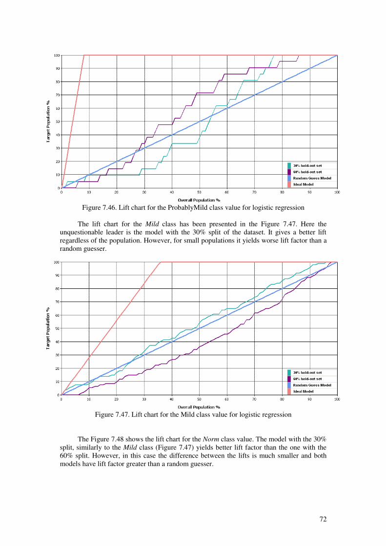
The lift chart for the Mild class has been presented in the Figure 7.47. Here theunquestionable leader is the model with the 30% split of the dataset. It gives a better liftregardless of the population. However, for small populations it yields worse lift factor than arandom guesser.

The Figure 7.48 shows the lift chart for the Norm class value. The model with the 30%split, similarly to the Mild class (Figure 7.47) yields better lift factor than the one with the60% split. However, in this case the difference between the lifts is much smaller and bothmodels have lift factor greater than a random guesser.

Figure 7.46. Lift chart for the ProbablyMild class value for logistic regression

Figure 7.47. Lift chart for the Mild class value for logistic regression

72

The Microsoft Logistic Regression yielded similar results to the neural network. Thisis because this algorithm is a realized with the use of the Microsoft Neural Network. Here,also the 30% split method turned out to be the best in all but two cases (when it comes to thelift factor). The two cases which favor the 60% split are the Malignant and the ProbablyMild

class values. The logistic regression models have worse results when it comes to the trueclass values. None of them predicted any of the instances from the Malignant, Suspicious

and ProbablyMild classes correctly. However, overall best model is the one with 30% splitof the dataset.

7.8 Microsoft Naive Bayes

The model of the Naive Bayes was built with the default setting of the parameters. Thetests have shown that the outcome of the method is not affected by the modification of theparameters, because they mostly concern the number of attributes and states.

The Table 7.15 presents the classification matrix of the method. At a first glimpse theerrors of predictions for Mild and Norm classes are slightly smaller than in case of theprevious algorithms. The Malignant class has been misclassified for all of its instances. Thesame situation is for the Suspicious and the ProbablyMild classes. Poor results were obtainedfor the Mild class as well as high proportion of predictions favored the Norm class. TheNorm value yielded good results as most of the instances were predicted correctly.

Table 7.15. Classification matrix for the Microsoft Naive Bayes

Predicted Malignant

(Actual)

Suspicious

(Actual)

ProbablyMild

(Actual)

Mild

(Actual)

Norm

(Actual)

Malignant 0 0 0 0 0

Suspicious 0 0 0 0 0

ProbablyMild

0 0 0 1 0

Mild 0 0 4 37 23

Norm 1 19 17 56 105

Figure 7.48. Lift chart for the Norm class value for logistic regression

73

THE EVALUATION OF THE NAIVE BAYES MODEL

The Table 7.16 shows the true class values rate generated by the Naive Bayes. This isthe only model which predicted all of the Malignant instances correctly. The worst resultswere gained for the Malignant, Suspicious and the ProbablyMild class value.

Table 7.16. True class values rates delivered by the Naive Bayes model

Model Malignant Suspicious ProbablyMild Mild Norm

Naive Bayes 0,00% 0,00% 0,00% 39,36% 82,03%

The lift charts for each of the class value are depicted in the Figures: 7.49, 7.50, 7.51,7.52 and 7.53.

The Figure 7.49 shows the lift chart for the Malignant class value. The Naive Bayesyielded a model which misclassified all of the Malignant instances. The reason for this maybe the poor representation of this value.

The lift chart for the Suspicious class value has been shown in the Figure 7.50. TheNaive Bayes gives a high lift factor which is always better than the random guesser's.

Figure 7.49. Lift chart for the Malignant class value for Naïve Bayes

74

The Figure 7.51 shows the lift chart for the ProbablyMild class. In this case the liftfactor is smaller than in case of the previous class. It even falls below the plot of the randomguesser. It is not worth using this algorithm for small and medium populations as it givesworse results than the random model.

The Figure 7.52 presents the lift chart for the Mild class. In this case the model yields

higher lift compared to the previous class. It is always higher than the random guesser.

Figure 7.50. Lift chart for the Suspicious class value for Naïve Bayes

Figure 7.51. Lift chart for the ProbablyMild class value for Naïve Bayes

75

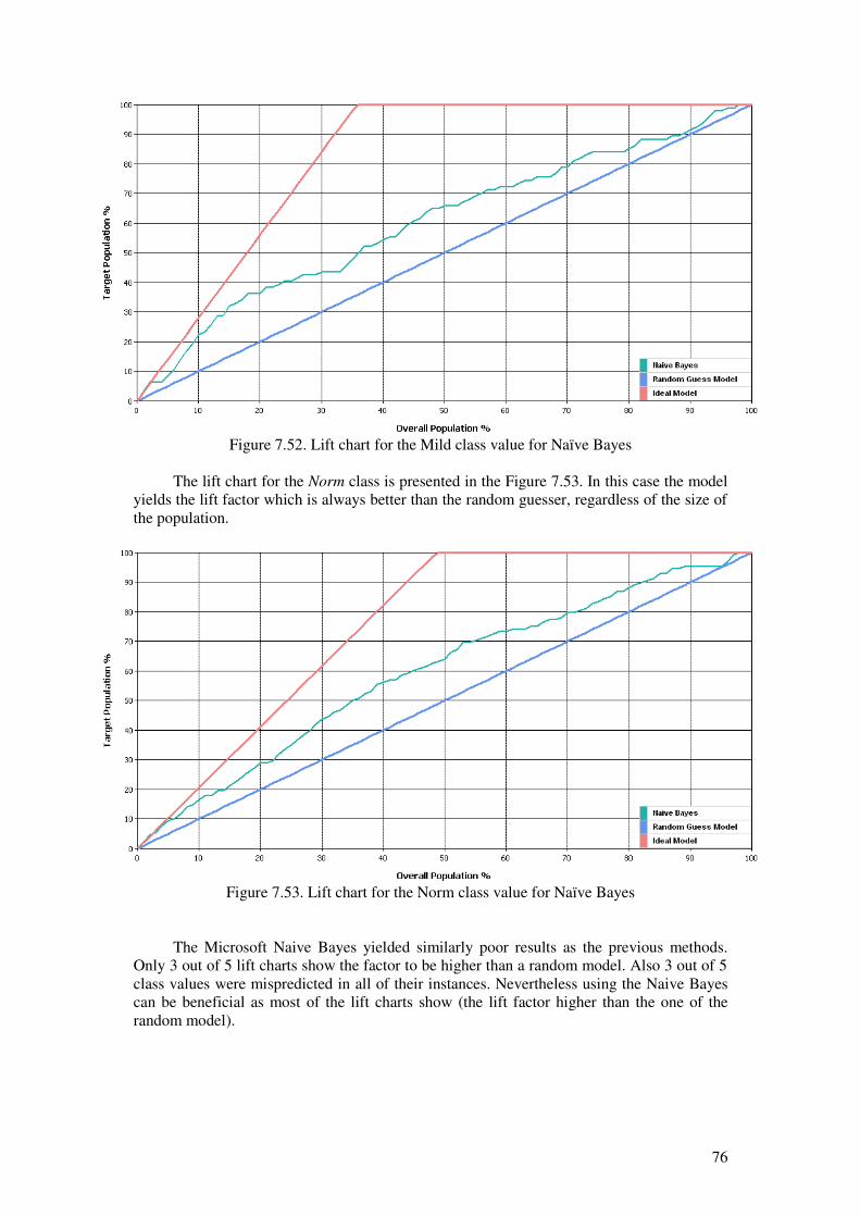
The lift chart for the Norm class is presented in the Figure 7.53. In this case the modelyields the lift factor which is always better than the random guesser, regardless of the size ofthe population.

The Microsoft Naive Bayes yielded similarly poor results as the previous methods.Only 3 out of 5 lift charts show the factor to be higher than a random model. Also 3 out of 5class values were mispredicted in all of their instances. Nevertheless using the Naive Bayescan be beneficial as most of the lift charts show (the lift factor higher than the one of therandom model).

Figure 7.53. Lift chart for the Norm class value for Naïve Bayes

Figure 7.52. Lift chart for the Mild class value for Naïve Bayes

76

7.9 Microsoft Association Rules

Similarly to the Microsoft Naive Bayes, also the Microsoft Association Rules weregenerated with the default parameters settings.

The Table 7.17 presents the classification matrix for the association rules. All of theinstances from the Malignant class have been misclassified. Good results were yielded forthe Suspicious and Norm classes, i.e. most of the predictions were correct. In case of theProbablyMild and the Mild values most of the predictions were wrong. However, unlike theprevious models at least some of the instances were correctly classified.

Table 7.17. Classification matrix for the association rules

Predicted Malignant

(Actual)

Suspicious

(Actual)

ProbablyMild

(Actual)

Mild

(Actual)

Norm

(Actual)

Malignant 0 0 0 0 0

Suspicious 0 13 2 46 22

ProbablyMild

0 0 1 14 6

Mild 0 5 12 17 26

Norm 1 1 6 17 74

THE EVALUATION OF THE ASSOCIATION RULES

The Table 7.18 shows the true class values rate generated by the association rules. Themodel delivered results better than previous models. For all but one of the class values atleast some of the instances were correctly classified. For two (Suspicious and Norm) morethan half of the instances were predicted correctly. This is the best overall result among all ofthe models constructed within the research.

Table 7.18. True class values rates delivered by the association rules model

Model Malignant Suspicious ProbablyMild Mild Norm

Association rules 0,00% 68,42% 4,76% 18,09% 57,81%

Here also the lift charts for each if the class values have been created. They aredepicted in the Figures 7.54, 7.55, 7.56, 7.57 and 7.58.

The Figure 7.54 presents the lift chart for the Malignant class value. The modelmisclassified all of the Malignant instances and thus the lift plot being far below the plot ofthe random guesser. The reason for this may be fact that this class is very poorly representedand the support of the rules containing this class was very low.

77

The Figure 7.55 shows the lift chart for the Suspicious class value. In this case the liftis significantly better than for the Malignant class. A very good lift factor has been gainedfor the percentage of population between 8% and 69. There is a long horizontal segment inwhich the lift factor does not grow. This means that taking a population of the size of 26% isno better than taking a 90% population.

The Figure 7.56 presents the lift chart for the ProbablyMild class. Here the situation issimilar: the best lift is gained for medium percentage of population (between 18% and 92%).However between 22% and 80% the lift factor equals zero.

Figure 7.54. Lift chart for the Malignant class value for association rules

Figure 7.55. Lift chart for the Suspicious class value for association rules

78

The lift chart for the Mild class value has been presented in the Figure 7.57. The lift inthis case is more monotonous in comparison with the previous ones for this model. There areless sudden “jumps” of the line. Almost entire line is over the plot of the lift of the randomguesser.

The Figure 7.58 shows the lift chart for the Norm class. The lift line crosses the line ofthe random guesser. Depending on the size of the population the use of the model may not bebeneficial.

Figure 7.56. Lift chart for the ProbablyMild class value for association rules

Figure 7.57. Lift chart for the Mild class value for association rules

79

None of the lift charts show a line that is completely above the line of the randommodel. All of the lift plots are either entirely below it (the Malignant class) or cross itoccasionally. This means that use of the association rules may not be beneficial for some ofthe populations. It may be worth trying the random guesser instead of the model.

7.10 Evaluation of the algorithms

The last step of the analyses is the comparative evaluation of the generated models.For the evaluation only the “best” models from their groups were taken, i.e. those thatyielded the best results in terms of the lift and the classifications. The following models havebeen chosen: – the decision tree built with the use of the entropy score method, – the clusters generated with the use of the EM algorithm, – the neural network with the 30% split of the dataset– the logistic regression with the 30% split of the dataset– the Naive Bayes, – the association rules.

The evaluation is performed in two stages. The first is based on the classificationmatrices generated for all of the models, not just those with the best lift (for bettervisualization presented in the Figure 7.59). The second compares the lift charts constructedonly for the best models. The Figures 7.60, 7.61, 7.62, 7.63 and 7.64 show the lift charts ofall of the models chosen for the evaluation with respect to the class values.

Figure 7.58. Lift chart for the Norm class value for association rules

80

The Figure 7.59 shows that the best results were gained for the Norm class value; theworst for the Malignant. This is because of the distribution of these values. The former hasthe most instances while the latter the least. The best results for the Suspicious and theProbablyMild classes have been gained with the use of the association rules. The modelswhich gave the worst results in terms of the classification are the 60% split neural networkand the logistic regression with the same split. They mispredicted not only the Malignant

class but also the Suspicious and ProbablyMild ones. Good results in terms of theclassification were obtained by the models: entropy tree, 30% split neural network and theassociation rules. For most of the class values they yielded correct prediction for at leastsome of the instances.

The Figure 7.60 presents the lift chart for the Malignant class value. All of the modelsmisclassified the only Malignant test instance (see Table ). However, the lift plots for all buttwo models (the association rules and the Naive Bayes) yielded high lift factors. This meansthat they were much less confident that the prediction was correct than the other two models.In this case the association rules and the Naive Bayes gave the worst results because theywere more confident that the wrong prediction was correct.

Figure 7.60. Comparative lift chart of all of the models with respect to the Malignant class value

Figure 7.59. Comparison of the classification matrices of all the models

81

En

trop

y tre

e

BK

2 tre

e

BD

EU

tre

e

EM

clu

ste

rs

K-m

ean

s c

luste

rs

NN

30

% s

plit

NN

60

% s

plit

LR

30

% s

plit

LR

60

% s

plit

Naiv

e B

ayes

Associa

tion

ru

les

0,00%

10,00%

20,00%

30,00%

40,00%

50,00%

60,00%

70,00%

80,00%

90,00%

100,00%

Malignant Suspicious ProbablyMild Mild Norm

The lift charts for the Suspicious class value have been presented in the Figure 7.62.Most of the models yielded the lift factor greater than the randomly guessed model. Threemodels' plots: the entropy tree, EM clusters and the association rules fell below the randomguesser. Good results were obtained for the neural network (with 30% split of the dataset)and the logistic regression (with the same split). From the models which have the lift plotabove the random guesser they give the best lift factor for almost entire population. Theworst model is the entropy tree. Its lift factor is way below the plot of the random guesser foralmost entire population.

The Figure 7.62 presents the lift charts for the ProbablyMild class value. The modelwhich yields the best lift is definitely the entropy decision tree. It reaches the 100%correctness of classification much sooner than other models. The second best model are theassociation rules. However, in this case the plot has a long horizontal line which depicts zerolift. The worst model in the case of this class are the EM clusters. They yield the lowest liftfrom all of the models, especially for small populations (less than 48% where the targetpopulation has no instances). The rest of the models delivered similar lift charts across theentire population. For small populations, though, their plots fall below the plot of the randomguesser.

Figure 7.61. Comparative lift chart of all of the models with respect to the Suspicious class value

82

The lift charts for the Mild class have been plotted in the Figure 7.63. The modelswhich got the best lift factors are the EM clusters and the association rules. The plots areinterspersed. The worst model turned out to be the entropy decision tree. Its plot falls belowthe plot of the random guesser, especially for small populations. The rest of the models gavesimilar charts.

The Figure 7.64 presents the lift charts for the Norm class. In this case the entropydecision tree also belongs to the worst models. Its plot also falls below the random model.The best model in this case are the EM clusters. Also the Naive Bayes proves to bebeneficial for small populations. The association rules can be employed only for smallpopulations as well. The rest of the models again have similar plots.

Figure 7.62. Comparative lift chart of all of the models with respect to the ProbablyMild class value

Figure 7.63. Comparative lift chart of all of the models with respect to the Mild class value

83

To sum up, it is impossible to choose one model which could suit all of the instances.Some model proved to give better results for only some class values, or only for populationsof certain size. There is no unquestionable leader among the models. Definitely, the bestmodels include the neural network, logistic regression both built with the 30% split of thedataset. These two gave lift which was better from the one delivered by the random guessedmodel. This means that is can be beneficial to use them. It may also be worth trying theassociation rules and the Naive Bayes. The former, even though its lift plot is often worsethan the one of the random guesser, it gave good results for 3 out of 5 class values, just likethe Naive Bayes.

7.11 Conclusions from the evaluation

The very important aspect of the data mining is the quality of the data. As shownin the graphs in the initial analyses (section 7.1) the distribution of the values of the attributesis mostly unequal. This in particular concerns the values of the class (theDiagnosisDescription). First and foremost, it takes 5 different values. In most of the researchdescribed in the Chapter 2 the classes took only two values (Boolean) which indicatedwhether an instance was benign or malignant. In the case of this research such classificationwas not possible due to the fact that the surveys did not deliver such information. None ofthe patients' cases have been ultimately assigned to either benign or malignant group. Thusthe only value that could be adopted as a class was the final mammography assessment. Asmentioned in the Chapter 5 often one mammography is not enough to decide about themalignancy of a case. This situation posed a serious problem to the learning methods. Someof the cases turned out to be so similar that often a model “confused” them, for instance theMild cases with the Norm ones and vice-versa.

Considerable differences in the number of instances belonging to each of the classescaused a situation in which not enough information was provided for the algorithms to learnparticular classes, e.g. the Malignant class. This resulted in the models which mispredictedthis value completely. Furthermore, most of the models provided low true class values rates.This must have also resulted from the resemblance of the instances. The unequal distributionof the class values also did not allow for applying the accuracy as a measure of the models'performance (for the reasons described in the Chapter 3) but required to use more advancedtechniques: lift charts and true class values rates (the environment does not implement anyother measures).

Figure 7.64. Comparative lift chart of all of the models with respect to the Norm class value

84

The evaluation of the data mining algorithms has shown that it is impossible to decidewhich is the best, i.e. the most suitable for the given dataset. The performance of the modelsvaried, depending on a class value. As mentioned previously, the models which gave the bestresults included: artificial neural network, logistic regression, association rules and the NaiveBayes. The first two had similar lift charts in most of the cases. This is because both methodsare realized with the use of a neural network. However, care needs to be given whileapplying them to future instances as they may give worse results than a random guessedmodel for some class values and populations. When the association rules are considered theygave decent results for most of the classes as their lift was above the lift of the randomguesser for most of the populations. This may be the result of the fact that the item setsextracted from the dataset had the support high enough. If the support was too high the itemsets would not be informative enough to generate good rules. However, even in the case ofthe association rules the lift sometimes falls below the random guesser's. Similar situation isfor the Naive Bayes. Even though this method delivered decent results for most of the classvalues its lift also falls below the lift of the random guesser for some classes and populations.

On the other hand, it is also very difficult to say which of the models not to usedefinitely. Probably the one to name would be the entropy decision tree as it had low liftfactor for most of the class values. This may results from the fact that the tree was verycomplex which could mean that it was over-trained.

Good results, in terms of the lift were also gained by the EM clusters. On most of thelift charts their lift was higher than of the random guesser at least for some populations.However, the clusters often also gave the lift significantly worse than the random guesser.This is probably also the effect of the poor quality of the training data. Since the EMalgorithm represents the soft clustering, some of the values must have been assigned toseveral clusters. This contributes the most to the low probabilities of belonging to a certaingroup, thus low confidentiality of predictions.

The worst results, though, were gained for the methods that have not been takenfor the final evaluation: k-means clusters, BK2 and BDEU trees, neural network and thelogistic regression model with 60% split of the dataset. In case of the k-means clusters, sincein the implementation the method still uses the probabilities the reasoning is the sameas for the EM clusters. The reason that the k-means clusters were worse than the EM onescan also result from the choice of the initial centers of the clusters. This delivered a modelthat gives poorer results than the EM one.

When it comes to the trees, the Bayesian score methods proved to give less accuratemodels probably because of the small size of the generated trees. Small number of leavescorresponds to a small number of rules and thus to a high number of misclassifications.

The neural network and the logistic regression models, which were built with the useof the 60% split of the dataset gave slightly poorer results than their counterparts builtwith the 30% splits. Here the reason may be the statistical distribution of the values.Probably 40% of the training examples was not enough to train a good network in bothcases: the Microsoft Neural Network and the Microsoft Logistic Regression (which is also aneural network in this case). This was discussed in the section 7.6. A conclusion was drawnthat both the training set and the testing set are of significant importance during the trainingof a data mining model. Comparable results obtained for both of the splits and the fact that60% split model was better for some class values than the 30% one implies that the sizes ofthese sets may not necessarily yield completely different models in terms of theperformance. However, the splits were done randomly, thus it is highly probable thatperforming the analyses for a couple more times may give different results. It may be alsoworth trying the 50% split of the dataset. Nevertheless, the results show that it may bedifficult to balance the division of the dataset into the training and the testing ones.Sometimes it may turn out that the testing set may serve its purpose well, but the training onewill yield a poor model or vice-versa.

The evaluation of the data mining models was also limited by the environment used.The Microsoft did not implement evaluation techniques commonly used in medicine [20] –the area under the ROC curves (AUC). However, the main orientation of the SQL Server

85

2005 is business [28] and in the implementation the system allows for incorporating costsinto the lift charts. Nevertheless, even business people would like to see which of the modelsprovide the best predictions. Implementing only one method may not be enough.

86

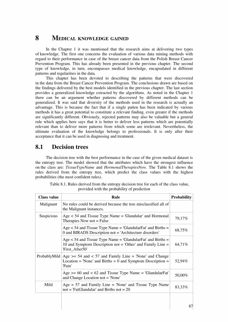
8 MEDICAL KNOWLEDGE GAINED

In the Chapter 1 it was mentioned that the research aims at delivering two typesof knowledge. The first one concerns the evaluation of various data mining methods withregard to their performance in case of the breast cancer data from the Polish Breast CancerPrevention Program. This has already been presented in the previous chapter. The secondtype of knowledge, in turn, encompasses medical knowledge, encapsulated in differentpatterns and regularities in the data.

This chapter has been devoted to describing the patterns that were discoveredin the data from the Breast Cancer Prevention Program. The conclusions drawn are based onthe findings delivered by the best models identified in the previous chapter. The last sectionprovides a generalized knowledge extracted by the algorithms. As noted in the Chapter 1there can be an argument whether patterns discovered by different methods can begeneralized. It was said that diversity of the methods used in the research is actually anadvantage. This is because the fact that if a single patten has been indicated by variousmethods it has a great potential to constitute a relevant finding, even greater if the methodsare significantly different. Obviously, rejected patterns may also be valuable but a generalrule which applies here says that it is better to deliver less patterns which are potentiallyrelevant than to deliver more patterns from which some are irrelevant. Nevertheless, theultimate evaluation of the knowledge belongs to professionals. It is only after theiracceptance that it can be used in diagnosing and treatment.

8.1 Decision trees

The decision tree with the best performance in the case of the given medical dataset isthe entropy tree. The model showed that the attributes which have the strongest influenceon the class are: TissueTypeName and HormonalTherapiesNow. The Table 8.1 shows therules derived from the entropy tree, which predict the class values with the highestprobabilities (the most confident rules).

Table 8.1. Rules derived from the entropy decision tree for each of the class value,provided with the probability of prediction

Class value Rule Probability

Malignant No rules could be derived because the tree misclassified all ofthe Malignant instances.

Suspicious Age < 54 and Tissue Type Name = 'Glandular' and HormonalTherapies Now not = False

79,17%

Age < 54 and Tissue Type Name = 'GlandularFat' and Births =0 and BIRADS Description not = 'Architecture disorders'

68,75%

Age < 54 and Tissue Type Name = 'GlandularFat' and Births =10 and Symptom Description not = 'Other' and Family Line ='First_After50'

64,71%

ProbablyMild Age >= 54 and < 57 and Family Line = 'None' and ChangeLocation = 'None' and Births = 0 and Symptom Description ='Pain'

52,94%

Age >= 60 and < 62 and Tissue Type Name = 'GlandularFat'and Change Location not = 'None'

50,00%

Mild Age = 57 and Family Line = 'None' and Tissue Type Namenot = 'FatGlandular' and Births not = 20

83,33%

87

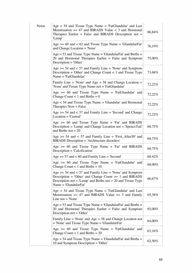
Norm Age < 54 and Tissue Type Name = 'FatGlandular' and LastMenstruation >= 47 and BIRADS Value < 3 and HormonalTherapies Earlier = False and BIRADS Description not ='Lump'

86,84%

Age >= 60 and < 62 and Tissue Type Name = 'GlandularFat'and Change Location = 'None'

76,19%

Age = 53 and Tissue Type Name = 'GlandularFat' and Births =20 and Hormonal Therapies Earlier = False and SymptomDescription = 'Other'

75,00%

Age >= 54 and < 57 and Family Line = 'None' and SymptomDescription = 'Other' and Change Count < 1 and Tissue TypeName = 'FatGlandular'

73,68%

Family Line = 'None' and Age = 58 and Change Location ='None' and Tissue Type Name not = 'FatGlandular'

72,22%

Age >= 60 and Tissue Type Name = 'FatGlandular' andChange Count < 1 and Births = 0

72,22%

Age < 54 and Tissue Type Name = 'Glandular' and HormonalTherapies Now = False

72,22%

Age >= 54 and < 57 and Family Line = 'Second' and ChangeLocation = 'Central'

72,22%

Age >= 60 and Tissue Type Name = 'Fat' and BIRADSDescription = 'Lump' and Change Location not = 'SpenceTail'and Births not = 20

68,75%

Age >= 54 and < 57 and Family Line = 'First_After50' andBIRADS Description = 'Architecture disorders'

68,75%

Age >= 60 and Tissue Type Name = 'Fat' and BIRADSDescription = 'Calcification'

68,75%

Age >= 57 and < 60 and Family Line = 'Second' 68,42%

Age >= 60 and Tissue Type Name = 'FatGlandular' andChange Count < 1 and Births = 10

68,00%

Age >= 54 and < 57 and Family Line = 'None' and SymptomDescription = 'Other' and Change Count >= 1 and BIRADSDescription not = 'Lump' and Births not = 20 and Tissue TypeName = 'GlandularFat'

66,67%

Age < 54 and Tissue Type Name = 'FatGlandular' and LastMenstruation >= 47 and BIRADS Value >= 3 and FamilyLine not = 'None'

65,38%

Age = 53 and Tissue Type Name = 'GlandularFat' and Births =20 and Hormonal Therapies Earlier = False and SymptomDescription not = 'Other'

65,00%

Family Line = 'None' and Age = 58 and Change Location not= 'None' and Tissue Type Name = 'GlandularFat'

64,00%

Age >= 60 and Tissue Type Name = 'FatGlandular' andChange Count < 1 and Births = 20

63,16%

Age < 54 and Tissue Type Name = 'GlandularFat' and Births =10 and Symptom Description = 'Other'

62,50%

88

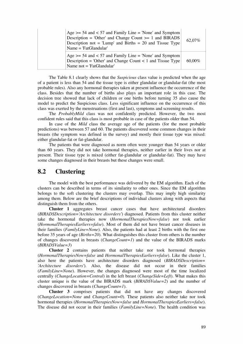
Age >= 54 and < 57 and Family Line = 'None' and SymptomDescription = 'Other' and Change Count >= 1 and BIRADSDescription not = 'Lump' and Births = 20 and Tissue TypeName = 'FatGlandular'

62,07%

Age >= 54 and < 57 and Family Line = 'None' and SymptomDescription = 'Other' and Change Count < 1 and Tissue TypeName not = 'FatGlandular'

60,00%

The Table 8.1 clearly shows that the Suspicious class value is predicted when the ageof a patient is less than 54 and the tissue type is either glandular or glandular-fat (the mostprobable rules). Also any hormonal therapies taken at present influence the occurrence of theclass. Besides that the number of births also plays an important role in this case. Thedecision tree showed that lack of children or one births before turning 35 also cause themodel to predict the Suspicious class. Less significant influence on the occurrence of thisclass was exerted by the menstruations (first and last), symptoms and screening results.

The ProbablyMild class was not confidently predicted. However, the two mostconfident rules said that this class is most probable in case of the patients older than 54.

In case of the Mild class the average age of the patients (for the most probablepredictions) was between 57 and 60. The patients discovered some common changes in theirbreasts (the symptom was defined in the survey) and mostly their tissue type was mixed:either glandular-fat or fat-glandular.

The patients that were diagnosed as norm often were younger than 54 years or olderthan 60 years. They did not take hormonal therapies, neither earlier in their lives nor atpresent. Their tissue type is mixed (either fat-glandular or glandular-fat). They may havesome changes diagnosed in their breasts but these changes were small.

8.2 Clustering

The model with the best performance was delivered by the EM algorithm. Each of theclusters can be described in terms of its similarity to other ones. Since the EM algorithmbelongs to the soft clustering the clusters may overlap. This may imply high similarityamong them. Below are the brief descriptions of individual clusters along with aspects thatdistinguish them from the others.

Cluster 1 aggregates breast cancer cases that have architectural disorders(BIRADSDescription='Architecture disorders') diagnosed. Patients from this cluster neithertake the hormonal therapies now (HormonalTherapiesNow=false) nor took earlier(HormonalTherapiesEarliers=false). Most of them did not have breast cancer diseases intheir families (FamilyLine=None). Also, the patients had at least 2 births with the first onebefore 35 years of age (Births=20). What distinguishes this cluster from others is the numberof changes discovered in breasts (ChangeCount=1) and the value of the BIRADS marks(BIRADSValue=3)

Cluster 2 contains patients that neither take nor took hormonal therapies(HormonalTherapiesNow=false and HormonalTherapiesEarliers=false). Like the cluster 1,also here the patients have architecture disorders diagnosed (BIRADSDescription=

'Architecture disorders'). Also, the disease did not occur in their families(FamilyLine=None). However, the changes diagnosed were most of the time localizedcentrally (ChangeLocation=Central) in the left breast (ChangeSide=Left). What makes thiscluster unique is the value of the BIRADS mark (BIRADSValue=2) and the number ofchanges discovered in breasts (ChangeCount=1).

Cluster 3 comprises patients that did not have any changes discovered(ChangeLocation=None and ChangeCount=0). These patients also neither take nor tookhormonal therapies (HormonalTherapiesNow=false and HormonalTherapiesEarliers=false).The disease did not occur in their families (FamilyLine=None). The health condition was

89

diagnosed normal (DiagnosisDescription=Norm). The lack of changes distinguishes thiscluster among others.

Cluster 4 aggregates patients that neither take nor took hormonal therapies(HormonalTherapiesNow=false and HormonalTherapiesEarliers=false). However, in theircases big-sized changes have been diagnosed (ChangeSize=5-14). The change was mostly alump (BIRADSDescription=Lump). The disease was not diagnosed in their families(FamilyLine=None). These changes diagnosed make the cluster unique among others.

Cluster 5 contains patients that do not take hormonal therapies not(HormonalTherapiesNow=false) but used to take them in the past(HormonalTherapiesEarlier=true). The changes discovered in their breasts were mostlyarchitectural disorders (BIRADSDescription='Architecture disorders'). Usually they hadmore than one child, the first one before 35 years of age (Births=20). The disease did notoccur in their families. What makes this cluster unique is the number of changes(ChangeCount=1) and the value of the BIRADS marks (BIRADSValue=2).

Cluster 6 contains patients that neither take not took hormonal therapies(HormonalTherapiesNow=false and HormonalTherapiesEarliers=false). The disease did notoccur in their families. However, the changes diagnosed in their breasts were of highdimensions (ChangeSie=5-14) and mostly it was a lump (BIRADSDescription=Lump). Whatdistinguishes this cluster from others is the number of changes discovered(ChangeCount=1).

Cluster 7 comprises patients that neither take nor took hormonal therapies(HormonalTherapiesNow=false and HormonalTherapiesEarliers=false). The disease wasnot diagnosed in their families (FamilyLine=None). The tissue type is mostly fat-glandular(TissueTypeName=FatGlandular). The usual BIRADS value was 3 (BIRADSValue=3).What distinguishes this cluster from others is the high average size of a change discovered inthe breasts (ChangeSize=14-40).

Cluster 8 contains patients who either had not changes diagnosed(ChangeLocation=None and ChangeCount=0) or had architecture disorders(BIRADSDescription='Architecture disorders'). The patients neither take nor took hormonaltherapies (HormonalTherapiesNow=false and HormonalTherapiesEarliers=false). Whatdistinguishes this cluster from others is the fact that usually there were no changesdiscovered in the breasts (ChangeCount=0).

Cluster 9 aggregates patients that had at least 2 children and the first one was beforethey turned 35 (Births=20). The patients neither take nor took hormonal therapies(HormonalTherapiesNow=false and HormonalTherapiesEarliers=false). The average age ofthe patients is 45-53 (Age=45-53). Mostly they had architecture disorders diagnosed(BIRADSDescription='Architecture disorders'). What distinguishes this cluster from theothers is the fact that the patients still have the menstruation (LastMenstruation=75-100).

Cluster 10 contains patients who neither take nor took hormonal therapies(HormonalTherapiesNow=false and HormonalTherapiesEarliers=false). Their type of thetissue is mostly glandular-fat (TissueTypeName=GlandularFat). They had only one childbefore they turned 35 (Births=10). They had their last menstruation between 45 and 53 yearsof age (LastMenstraution=45-53). Their average age is 45-53 (Age=45-53). Whatdistinguishes this cluster from the others is the fact that mostly the changes discovered werebig (ChangeSize=15-40). The number of these changes was between 3 and 5(ChangeCount=3-5).

Unlike the decision trees (section 8.1.) the clusters do not provide such confidentpredictions (the number of instances from none of the classes exceeds 50% in any of theclusters). Thus, for the purpose of the medical knowledge extraction, only the clusters whichcontain at least 30% of instances from a given class were analyzed. The Table 8.2 showsthese clusters along with class value and the distribution.

90

Table 8.2. Distributions (at least 30%) of class values in particular clusters

Class value Cluster number Distribution

Malignant No cluster contains at least30% of malignant instances

Suspicious 10 0,32

ProbablyMild 10 0,36

8 0,30

Mild 1 0,42

2 0,46

4 0,42

6 0,51

7 0,42

9 0,44

Norm 1 0,47

2 0,43

3 0,73

4 0,49

5 0,54

7 0,33

8 0,38

9 0,36

Despite the fact that the EM clusters gave poor results their profiles and the Table 8.2allow for drawing some medical conclusions. The Suspicious or the ProbablyMild classes(the same cluster) were observed in the patients of about 53 years of age, after themenopause. They usually do not take any hormonal therapies but had several relatively largechanges diagnosed in their breasts. Often the disease had been diagnosed in their families.

When it comes to the Mild class value the patients mostly had some change in theirbreasts diagnosed: architecture disorders or lump for the most times. The average age wasbetween 51 and 57 years. Some of the patients took hormonal therapies (earlier and atpresent) other did not. The tissue type was mixed. Most of the time it was the glandular-fat,however, a small proportion had the fat-glandular type.

The Norm class encompasses the patients who either did not have any changesdiagnosed or the changes had small intensity (BIRADSValue)

8.3 Neural network

The results delivered by the neural network are presented in the Table 8.3. The tableshows which attribute/value pairs favor the class values. In other words, inputting the valuesof the attributes from the right column of the table to the network will most likely (thehighest probability) make it predict the classes from the left column, regardless of otherinputs. The Table 8.3 has been constructed according to the following steps (established afterseveral tests), the validity of these findings were verified in the Microsoft SQL Server 2005:

1. For every pair of class values generate a list of attribute/value pairs that favor eachof the class values

91

2. Eliminate those attribute/value pairs that are duplicated in at least two class valuesfavoring only one of them.

3. For each class value, for each attribute whose 2 or more values have been added tothe set check if all of them actually favor the class value. Remove those that do not.

These simple steps allowed for creation of one of the possible input attribute/value pairsets for each of the class value. Certainly, there can be more sets like this and this algorithmseeks for the first solution.

Table 8.3. Impact of the attributes' values on the class value for the neural network

Class value Attribute/value pair which favors the class value

Malignant Births=21, FamilyLine='Second',SymptomDescription={'Nipple inversion', 'Surgery','Skin disorders'},TissueTypeName='Glandular'

Suspicious BIRADSDescription='Calcification',Births='0',ChangeSize='4,711-14,616'FamilyLine='First_After50',TissueTypeName='Glandular', SymptomDescription='Skin disorders'

Probably mild Births='10', ChangeSize='4,711-14,616', FamilyLine='First_Before50',SymptomDescription={'Mastopathy', 'Lump', 'Skin disorders'}

Mild Age='59,940-70,000'Births='0',SymptomDescription='Mastopathy',ChangeLocation='SpenceTail'FamilyLine='First_Before50'

Norm Age='59,940-70,000', Births='11', FamilyLine={'First_Before50', FamilyLine='Second'}, SymptomDescription='Surgery', TissueTypeName='Fat'

The most influential attributes that make the network classify an instance as Malignant

is the number of births (2 children, first one after 35 years of age) and the tissue type(glandular). Also two of the symptoms are influential: nipple inversion and skin disorders.

In case of the suspicious instances the tissue type was also glandular. However, in thiscase the patients often did not have any children. The changes diagnosed in their breastswere usually large and mostly it was the calcification. Also close relatives after 50 years ofage had the breast cancer.

As for the ProbablyMild class the most influential attribute was the number of births(one child before 50 years of age) and also the size of the change discovered in the patient'sbreasts (usually large) located mostly in the so-called Spence's tail. Similarly to thesuspicious cases the close relatives suffered from the disease before they turned 50.

The normal cases concerned women between 60 and 70 years of age. They usually hadtheir only children after the turned 35 years old. What is surprising, the disease wasdiagnosed in their families, both in close and distant relatives.

92

8.4 Logistic regression

The Table 8.4 shows the impact of the particular attributes' values on the class value.The table has been prepared according the same steps as in case of the neural networks.

Table 8.4. Impact of the attributes' values on the class value for the logistic regression

Class value Attribute/value pair which favors the class value

Malignant Births='11',ChangeSize='4,711-14,616',FamilyLine='First_After50',SymptomDescription='Skin disorders',TissueTypeName='Fat'

Suspicious BIRADSDescription='Calcification',Births='0',ChangeSize='4,711-14,616', FamilyLine='First_After50',HormonalTherapiesNow='True',TissueTypeName='Glandular',SymptomDescription='Skin disorders',

Probably mild Births='10',ChangeSize='4,711-14,616', FamilyLine='First_Before50', SymptomDescription={'Lump', 'Skin disorders'},

Mild Births={'21', '0'},FamilyLine='First_Before50',SymptomDescription='Nipple inversion',TissueTypeName='Glandular'

Norm Births='11', FamilyLine='Second',HormonalTherapiesNow='True', SymptomDescription={'Surgery', 'Skin disorders'},TissueTypeName='Fat'

The logistic regression, even though it is realized with the neural network, deliveredslightly different results than the neural network. As far as the Malignant class is concerned,the number of births is also an influential factor (however, in this case only one child, after35 years of age). Also, the changes discovered in the patients' breasts were large and theyhad some skin disorders. Their tissue was fat-based. The disease has been diagnosed in theclose relatives after 50 years of age.

When it comes to the suspicious cases the size of the changes and the presence of theskin disorders is the same as in the malignant ones. The difference is in the fact that thepatients now apply the hormonal therapies and they did not have any children. Their tissuetype is glandular. The disease has been diagnosed in the close relatives after 50 years of age.

Also the changes were large in case of the ProbablyMild class. Similarly to the twoprevious cases, the disease has been discovered in the close relatives, but before they turned50 years old.

The women, who were diagnosed as Mild, often either did not have any children orhad 2 after they turned 35 years old. Their tissue type was usually glandular.

The Norm class, as conveyed by the model, usually had the fat tissue type. Thepatients also had some skin disorders.

93

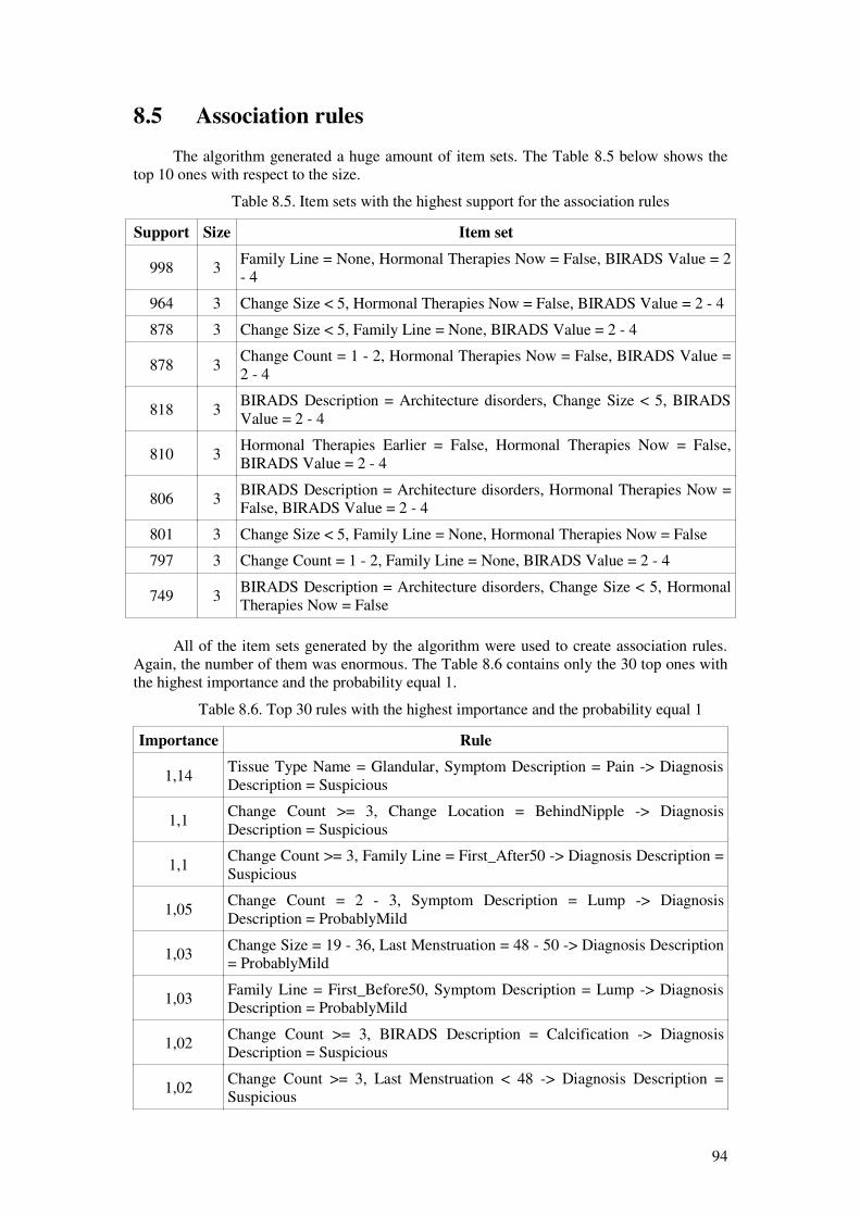
8.5 Association rules

The algorithm generated a huge amount of item sets. The Table 8.5 below shows thetop 10 ones with respect to the size.

Table 8.5. Item sets with the highest support for the association rules

Support Size Item set

998 3Family Line = None, Hormonal Therapies Now = False, BIRADS Value = 2- 4

964 3 Change Size < 5, Hormonal Therapies Now = False, BIRADS Value = 2 - 4

878 3 Change Size < 5, Family Line = None, BIRADS Value = 2 - 4

878 3Change Count = 1 - 2, Hormonal Therapies Now = False, BIRADS Value =2 - 4

818 3BIRADS Description = Architecture disorders, Change Size < 5, BIRADSValue = 2 - 4

810 3Hormonal Therapies Earlier = False, Hormonal Therapies Now = False,BIRADS Value = 2 - 4

806 3BIRADS Description = Architecture disorders, Hormonal Therapies Now =False, BIRADS Value = 2 - 4

801 3 Change Size < 5, Family Line = None, Hormonal Therapies Now = False

797 3 Change Count = 1 - 2, Family Line = None, BIRADS Value = 2 - 4

749 3BIRADS Description = Architecture disorders, Change Size < 5, HormonalTherapies Now = False

All of the item sets generated by the algorithm were used to create association rules.Again, the number of them was enormous. The Table 8.6 contains only the 30 top ones withthe highest importance and the probability equal 1.

Table 8.6. Top 30 rules with the highest importance and the probability equal 1

Importance Rule

1,14Tissue Type Name = Glandular, Symptom Description = Pain -> DiagnosisDescription = Suspicious

1,1Change Count >= 3, Change Location = BehindNipple -> DiagnosisDescription = Suspicious

1,1Change Count >= 3, Family Line = First_After50 -> Diagnosis Description =Suspicious

1,05Change Count = 2 - 3, Symptom Description = Lump -> DiagnosisDescription = ProbablyMild

1,03Change Size = 19 - 36, Last Menstruation = 48 - 50 -> Diagnosis Description= ProbablyMild

1,03Family Line = First_Before50, Symptom Description = Lump -> DiagnosisDescription = ProbablyMild

1,02Change Count >= 3, BIRADS Description = Calcification -> DiagnosisDescription = Suspicious

1,02Change Count >= 3, Last Menstruation < 48 -> Diagnosis Description =Suspicious

94

1,02Change Count >= 3, First Menstruation < 12 -> Diagnosis Description =Suspicious

1,02Change Count >= 3, Family Line = Second -> Diagnosis Description =Suspicious

0,98Change Size >= 36, Last Menstruation = 48 - 50 -> Diagnosis Description =ProbablyMild

0,98 Change Size >= 36, Births = 20 -> Diagnosis Description = ProbablyMild

0,98Change Size >= 36, Hormonal Therapies Now = False -> DiagnosisDescription = ProbablyMild

0,98Symptom Description = Skin disorders, Change Location = SpenceTail ->Diagnosis Description = ProbablyMild

0,96Symptom Description = Skin disorders, Age = 53 - 56 -> DiagnosisDescription = Suspicious

0,96Change Count = 2 - 3, BIRADS Description = Calcification -> DiagnosisDescription = Suspicious

0,96Change Size = 7 - 19, Change Count < 1 -> Diagnosis Description =Suspicious

0,96 Change Size = 19 - 36, Births = 0 -> Diagnosis Description = Suspicious

0,92Change Size >= 36, Tissue Type Name = Fat -> Diagnosis Description =ProbablyMild

0,92 Change Size >= 36, Age < 53 -> Diagnosis Description = ProbablyMild

0,92Change Size >= 36, First Menstruation = 13 - 14 -> Diagnosis Description =ProbablyMild

0,92Change Size >= 36, Symptom Description = Mastopathy -> DiagnosisDescription = ProbablyMild

0,92 Change Size >= 36, Age = 56 - 60 -> Diagnosis Description = ProbablyMild

0,92Change Size >= 36, Tissue Type Name = GlandularFat -> DiagnosisDescription = ProbablyMild

0,92Change Size >= 36, First Menstruation = 14 - 16 -> Diagnosis Description =ProbablyMild

0,92First Menstruation < 12, Symptom Description = Lump -> DiagnosisDescription = ProbablyMild

0,92Change Size >= 36, Symptom Description = Other -> Diagnosis Description= ProbablyMild

0,92First Menstruation < 12, Age = 60 - 65 -> Diagnosis Description =ProbablyMild

0,92Symptom Description = Skin disorders, First Menstruation >= 16 ->Diagnosis Description = ProbablyMild

0,43Family Line = First_Before50, Age = 56 - 60 -> Diagnosis Description =Mild

The item sets, with the highest support, delivered by the model are not informativeenough. The most frequent item set (BIRADSValue = 2-4) does not bring any newinformation other than the one presented in the initial analyses in the Chapter 7. However,the sets with little lower support do deliver some information. For instance, the lack of the

95

breast cancer disease in the family goes with the lack of the hormonal therapies at presentand the size of a change less than 5 mm.

The model mispredicted all of the malignant cases. In case of the suspicious ones theattribute which exerts the biggest influence on the class is the number of changes greater orequal 3.

The ProbablyMild cases are influenced the most by the size of a change, which isgreater than 36 mm.

When it comes to the mild cases the most influential attribute is the number of births.The patient usually had more than 1 one and the first delivery was after 35 years of age. Thesecond attribute is the nipple inversion symptom and the number of changes (1 or 2). Finally,the patients were usually 56 to 60 years old.

Finally, the normal cases encompass the patients that had a surgery in the area of thebreasts. They usually had only one child after they turned 35. They did not have any changesdiscovered.

8.6 Naive Bayes

The Naive Bayes discovered dependencies among the attributes. The dependenciesordered by the strength are as follows: ChangeCount, TissueTypeName,SymptomDescription, LastMenstruation, ChangeSize, HormonalTherapiesNow andBIRADSValue. These attributes have been analyzed with respect to their correlation with theclass values. The results of these analyses are presented in the Figures: 8.1, 8.2, 8.3, 8.4 and8.5. These figures show how often (expressed as a ratio of all the instances) each of theattributes appears with the particular class value. In case of the Malignant class (Figure 8.1)its occurrence is accompanied with several attributes. Examining the Figure 8.1 it is apparentthe Malignant class always goes with the Symptom Description (value Other), theTissueTypeName (value Fat), ChangeCount (value 1-2), BIRADSValue (value 2-4) and theHormonalTherapiesNow (value false).

The Analysis Services also allow to compare the attributes in terms of their influenceon the class value. When it comes to the Malignant the two most influential ones, whichfavor anything but this class are: ChangeSize < 5 and SymptomDescription = 'Nipple

Figure 8.1. The Malignant class value characteristics for the Naïve Bayes

ChangeSize = 5 - 7

LastMenstruation = 51 - 53

LastMenstruation = 48 - 50

ChangeSize = 7 - 19

HormonalTherapiesNow = False

BIRADSValue = 2 - 4

ChangeCount = 1 - 2

TissueTypeName = Fat

SymptomDescription = Other

0 0,1 0,2 0,3 0,4 0,5 0,6 0,7 0,8 0,9 1

96

inversion'. On the other hand the one which favors this class the most is the TissueTypeName

= Fat. The Figure 8.2 shows the correlations for the Suspicious state of the class. This class

always appears with the BIRADSValue set to the value 2-4. This value was also present inthe previous class (the Malignant). The reason for this is the fact that the internaldiscretization function generated only one value for this attribute, i.e. 2-4.

The Suspicious value is favored the most by the two attributes: LastMEnstruation =

51-53 and TissueTypeName = 'Glandular'. The third one is the ChangeCount >= 3. On theopposite side, favoring anything else but the Suspicious value, is the attributeTissueTypeName = 'FatGlandular'. The second and third are the LastMenstruation = 50-51and SymptomDescription = 'Other' respectively.

In case of the ProbablyMild (Figure 8.3) also the class always appears with theattribute BIRADSValue = 2-4, for the same reason as for the previous classes.

Figure 8.2. The Suspicious class value characteristics for the Naïve Bayes

ChangeSize = 19 - 36

SymptomDescription = Skin disorders

ChangeCount = 2 - 3

TissueTypeName = Fat

LastMenstruation = 50 - 51

ChangeSize = 5 - 7

LastMenstruation < 48

ChangeCount >= 3

LastMenstruation >= 53

Symptom Description Lump

LastMenstruation = 48 - 50

TissueTypeName = Glandular

HormonalTherapiesNow = True

ChangeCount < 1

ChangeSize = 7-19

SymptomDescription = Mastopathy

TissueTypeName = FatGlandular

SymptomDescription = Pain

SymptomDescription = Other

TissueTypeName = GlandularFat

LastMenstruation = 51 - 53

ChangeCount = 1 - 2

ChangeSize < 5

HormonalTherapiesNow = False

BIRADSValue = 2 - 4

0 0,1 0,2 0,3 0,4 0,5 0,6 0,7 0,8 0,9 1

97

When it comes to the influence the attributes exert on the class value, the mostinfluential one which favors this class is the LastMenstruation = 50-51. It is followed by theSymptomDescription = 'Lump'. However, the attribute SymtpomDescription = 'Other',favoring anything else but this class, is more influential than them. The next attribute whichfavor Not-ProbablyMild class value is the LastMenstruation < 48.

The Figure 8.4 shows the correlations between the attributes and the Mild class. Themost frequent attribute (besides the BIRADSValue = 2-4) is the HormonalTherapiesNow =

False.

Figure 8.3. The ProbablyMild class value characteristics for the Naïve Bayes

ChangeSize >= 36

SymptomDescription = Skin disorders

TissueTypeName = Fat

LastMenstruation < 48

ChangeSize = 5 - 7

HormonalTherapiesNow = True

ChangeSize = 19 - 36

ChangeCount = 2 - 3

LastMenstruation = 51 - 53

LastMenstruation = 48 - 50

ChangeSize = 7 - 19

SymptomDescription = Other

SymptomDescription = Pain

SymptomDescription = Lump

ChangeCount < 1

LastMenstruation >= 53

SymptomDescription = Mastopathy

LastMenstruation = 50 - 51

TissueTypeName = FatGlandular

TissueTypeName = GlandularFat

ChangeCount = 1 - 2

ChangeSize < 5

HormonalTherapiesNow = False

BIRADSValue = 2 - 4

0 0,1 0,2 0,3 0,4 0,5 0,6 0,7 0,8 0,9 1

98

In the case of the Mild class the most influential attribute which favors anything butthe Mild class value is the ChangeCount < 1. Its influence is stronger than the strongestinfluence of the attribute favoring the class, i.e. the ChangeCount = 1-2. The attributes:HormonalTherapiesNow = False also favors this class but is weaker than theHormonalTherapiesNow = True which, in turn, favors anything else but the Mild class value

The Figure 8.5 presents the correlations in case of the Norm class value. The mostfrequent ones are the same as for the Mild class, i.e. BIRADSValue = 2-4 andHormonalTherapiesNow = False.

Figure 8.4. The Mild class value characteristics for the Naïve Bayes

ChangeCount >= 3

ChangeSize = 19 - 36

TissueTypeName = Glandular

HormonalTherapiesNow = True

ChangeCount = 2 - 3

TissueTypeName = Fat

SymptomDescription = Lump

ChangeSize = 7 - 19

ChangeCount < 1

ChangeSize = 5 - 7

SymptomDescription = Pain

LastMenstruation = 50 - 51

LastMenstruation = 48 - 50

LastMenstruation = 51 - 53

LastMenstruation < 48

LastMenstruation >= 53

SymptomDescription = Mastopathy

TissueTypeName = GlandularFat

TissueTypeName = FatGlandular

SymptomDescription = Other

ChangeSize < 5

ChangeCount = 1-2

HormonalTherapiesNow = False

BIRADSValue = 2-4

0 0,1 0,2 0,3 0,4 0,5 0,6 0,7 0,8 0,9 1

99

The Norm class value is favored by three attributes: ChangeCount < 1,SymtpomDescription = 'Other' and ChangeSize < 5. Their influence is stronger than thestrongest one – the ChangeCount = 1-2 – which favors anything else but this class value. Yetanother attribute, which is in favor of the Norm class value is the TissueTypeName = 'Fat'.

According to what the Naive Bayes delivered the attributes which exert the mostimpact on the class value are the number of changes, tissue type and the symptoms. Also thelast menstruation and hormonal therapies play an important role in classification.

The malignant cases are always accompanied by symptom values other than thedefault ones specified in the surveys. Also, the tissue type is always fat. The number ofchanges is either 1 or 2. Also the model always associated the malignant cases with the factof lack of hormonal therapies applied by the patients.

When it comes to the suspicious cases the model was not that certain as in the previousclass. The occurrence of this class is highly connected with the lack of hormonal therapies.Also the number of changes is equal to 1 or 2 and their size is less than 5 mm. The patientshad their last menstruation at the age of 51 to 53. The type of their breast tissue is glandular-fat.

The ProbablyMild class almost always appears accompanied by the lack of hormonaltherapies. Similarly to the previous class, the number of changes is either 1 or 2 and theirsize is less than 5 mm. The tissue type is mixed though: either glandular-fat or fat-glandular,with the former being more probable.

Figure 8.5. The Norm class value characteristics for the Naïve Bayes

ChangeCount >= 3

SymptomDescription = Surgery

ChangeCount = 2 - 3

TissueTypeName = Glandular

SymptomDescription = Skin disorders

ChangeSize = 7 - 19

SymptomDescription = Lump

ChangeSize = 5 - 7

HormonalTherapiesNow = True

SymptomDescription = Pain

LastMenstruation = 48 - 50

TissueTypeName = Fat

SymptomDescription = Mastopathy

LastMenstruation < 48

LastMenstruation = 50 - 51

LastMenstruation >= 53

LastMenstruation = 51 - 53

ChangeCount < 1

TissueTypeName = GlandularFat

TissueTypeName = FatGlandular

SymptomDescription = Other

ChangeCount = 1 - 2

ChangeSize < 5

HormonalTherapiesNow = False

BIRADSValue = 2 - 4

0 0,1 0,2 0,3 0,4 0,5 0,6 0,7 0,8 0,9 1

100

The mild cases most likely will come also with the lack of the hormonal therapies. Thesize and the number of changes are equal to the previous cases. The model is less certainabout the tissue type.

The patients whose condition has been diagnosed as normal most likely did not applyhormonal therapies. The changes discovered in their breasts were smaller than 5 mm. Themost probable tissue type was the fat-glandular.

8.7 Generalization of the knowledge

All of the models delivered some knowledge about the breast cancer disease.However, the information is very vague and often contradictory with the one conveyed byother models. Nevertheless, an attempt has been made to generalize the premises in order tocome up with a small but concise set of facts.

One of the most influential attributes is the age. A significant proportion of theclassifications delivered by the models take it into consideration. Regularity has beenobserved that the group of women that has the highest risk of the breast cancer compriseswomen approximately between 50 and 57 years of age. According to what the modelsconvey the disease is much less likely to occur in older women.

Another important attribute, which has a large impact on the predictions, is the tissuetype. However, the models do not agree what types favor what class value. There is a slighttendency that the mixed tissues are more likely to develop the cancer.

Hormonal therapies are another influential attribute. It has been observed that applyingsuch a therapy increases the risk of going down with the disease. Most of the models did notmake any distinction whether the therapy was applied earlier or at present.

The disease in the family is also an influential factor. This concerns the close relativesin particular. It has been observed that occurrence of the disease in the family increasesthe risk of becoming ill.

The screening results proved to be less deterministic than expected. Any changes, eventhe big ones do not imply the disease.

101

9 CONCLUSIONS AND FUTURE WORK

The main goal of the research was to first and foremost analyze the data from thesurveys of the National Breast Cancer Prevention Program and to judge whether it is suitableto be analyzed with the use of the data mining methods. The second step was to evaluateseveral data mining algorithm in terms of their applicability to this data. Finally, an attemptwas made to deliver some tangible medical knowledge extracted by the methods. In generalthe research was to answer the following questions:

1. What is the quality of the medical dataset gathered from the Polish Breast Cancer

Prevention Program?

The quality of analytical data is very important to building good data mining models.The data used in this research came from the surveys filled out both by patients of theOncological Clinic in Wrocław, Poland, and the medical staff of the health care facility. Aspeople tend to do mistakes the data contained a lot of noise. During the ETL process vastmajority of the data had to be eradicated due to various inconsistencies and errors whichwere impossible to rectify. The resulting set contained attributes whose values were farunequally distributed. This poses a serious problem of insufficiency of training information.If a given attribute is poorly represented, not only will it fail to bring relevant informationbut also it may introduce additional noise.

The poor quality of the training data could also be the effect of possiblemisunderstandings of survey questions or many other factors related to the surveys.Obviously, it is impossible to eliminate all of these factors, however, it is feasible to limitthem. The survey form could be updated so that patients do not overlook questions, as ittakes place now in case of several questions located in wrong places (for instance the upperright corner of the form). The formulation (the wording) of the questions needs to target thesurvey-takers. Questions whose answers depend on some other questions (like the “age atfirst birth” depends on the “number of births”) should be clearly marked.

The very process of surveying also has a lot to be desired. The physicians fail to fillout the surveys after a screening has been completed. They tend to only attach a free-textnote describing the findings and leaving the survey's questions blank. This makes thereception of the data very difficult and often requires removing large portions of it.Nevertheless, despite the poor quality of the data it was used to conduct the analyses.

2. Which data mining methods can be applied to extract knowledge from the medical

dataset gathered from the Polish National Breast Cancer Prevention Program?

The second goal was to evaluate several data mining methods. Six of them werechosen because of their implementation in the target analytical environment: the businessintelligence part of the Microsoft SQL Server 2005. The models constructed in the learningprocess were evaluated with the use of lift charts and classification matrices. The results ofthe analyses proved that it is impossible to name one classifier which would be the best forthe given dataset. The reason for this situation is the poor quality of the training data. Noneof the models correctly classified the Malignant instances because there was not enoughtraining information to learn from. The models were, in a sense, “unaware” of this class. Itmay be advisable to try several of the algorithms prior to their application in real medicalsystems.

The models which yielded good results were: artificial neural network, logisticregression (both with the 30% split of the dataset), association rules and the Naive Bayes.They had the highest lift factor for most of the class values and also the true class value rateswere higher than in case of other models. Nevertheless, application of these methods requirescare because for some populations they gave results poorer than a random guesser. This

102

means that it is more beneficial to choose the instances randomly than to apply the method.The first two methods (neural network and logistic regression) had lift plots similar to eachother. In case of the association rules the item sets had “high-enough” support. This gavegood rules, however still only for some class values and for some populations. The samegoes for the Naive Bayes. Good results were also gained by the EM clusters. However, thecarefulness also applies here. This also results from the poor quality of the training data. Softclusters (as the EM cluster are) allows for a value to belong to several groups at once. Lowquality of the data could result in assignment of the values to a number of clusters. Thismeans low probability of belonging to any.

It is also difficult to say which of the methods could not be applied to the dataset (fromthose taken for the ultimate evaluation). The worst results were gained by the entropy tree.This may results from the over-training of the tree which was very complex. However, theresearch showed that definitely the worst methods, which should not be used, are thosewhich were not taken for the final evaluation: k-means clusters, BK2 and BDEU trees, neuralnetwork and logistic regression model with 60% split of the dataset. The k-means clusters,similarly to the EM ones in the SQL Server 2005 implementation use the probability ofbelonging to a group. Due to the low quality of the data, wrong clusters must have beenchosen for the attributes. Also the reason for poor performance of this method could be theinitial choice of the cluster centers. When it comes to the Bayesian trees (BK2 and BDEU)they were small. This could have been the reason for the low performance. The number ofattributes must have been too small to give good predictions. The neural network and thelogistic regression models, which were built with the use of the 60% split of the dataset gavepoorer results than their counterparts built with the 30% splits. The reasoning for such a splitwas to determine the impact of both the cardinality of the training and the testing sets on theoutput model. The analyses proved that the 30% split network gives slightly better results.This may have been due to the poor quality of the training data or simply because the othernetwork did not have enough information to train a good model. However, these resultsshow that the split of the dataset does not necessary influence the output model in asignificant way. The analyses have shown that large difference in the cardinality of both setsdoes not give considerably different results. This may have been due to the unequaldistributions of the class values, though as the performance of the model was probablyaffected the most by the majority class: the Norm value.

3. What knowledge (patterns) can the methods extract from the medical dataset

gathered from the Polish Breast Cancer Prevention Program?

The last step of the research was to deliver some tangible medical knowledge fromwhat the models extracted. The unanimousness of the predictions was used as a measure ofpotential relevance of the findings. If most of the models confirmed a premise, there was agood chance that it constituted some practical information. There is a discussion whethersuch a measure can be applied. The argument against it is the diversity of data miningmethods and the fact that each of them is different and treats data in a different way.However,on the other hand, such diversity can be regarded as an advantage, because apattern delivered by different methods has a great potential to be valuable and important.A rule applied in this research says that it is more beneficial to deliver a smaller set ofpatterns which are potentially relevant than to deliver a broader set of patterns from whichsome are irrelevant. The latter situation might have been encountered if all of the discoveredpatterns were taken into consideration as some of them were contradictory. On the otherhand, limiting the set of patterns to only the potentially relevant ones poses a threat ofremoving other potentially relevant ones. This is the cost which needs to be taken in order toprovide doctors with findings in an concise and comprehensive form. This trade-off wasmade to prevent the research from delivering too many patterns that is actually not deliveringanything at all.

Several correlations have been found. One of the most important is the strongassociation between the age of a patient and the breast cancer occurrence. The research has

103

indicated that women between 50 and 57 years of age are in the high-risk group, whereasolder ones are less susceptible to the disease. Another very influential facet is the type of thebreast tissue. However, when it comes to the values of this attribute the models were notunanimous. They agreed, though, on the significance of the hormonal therapies and theirimpact on a patient's health. Application of such a therapy, according to the most of themodels, increases the risk of going down with the breast cancer. The risk is also shifted if thedisease was diagnosed in the members of family, especially the close relatives.

What was a little surprising was that the screening results do not exert so muchinfluence on the diagnosis of the breast cancer as one might have expected. The presencechanges, their large size, quantity and location, do not necessarily mean the disease.

Despite the confidence of the above findings, they have to be validated by professionalphysicians. This research was only to point to some directions that potentially may bringsome new knowledge, which further developed, may turn out to be helpful. The patternsdiscovered by the data mining methods employed in the research are not supported by anymedical knowledge, though. They have been learned only by finding correlations amongattributes. Furthermore, the amount of training data was very small comparing to all of thepossible combinations of attributes' values. This also may have distorted the findings. It hasnot been an intention of the research to prove that data mining algorithms can be blindlyused in real life (especially in medicine). It was an intention, though, to point out theirpotential in directing people to possibly relevant and important knowledge that is hidden indata. This knowledge, and it also concerns this research, may turn out to be worthless andcompletely wrong. However, this has to be verified by knowledgeable people, who, unlikemachines, have broader knowledge and are capable of associating different premises anddrawing sophisticated conclusions.

The research will be carried on. The next step is the evaluation of the results by themedical staff of the Wroclaw health unit. In a more distant perspective the analyses alongwith the DataRetriever software tool will constitute a basis for development of a medicaldecision support system.

104

10 REFERENCES

[1] Abbass H. A., An Evolutionary Artificial Neural Networks Approach for Breast CancerDiagnosis, CiteSeer, 2002 [2] Appendix No. 4 of the disposition No. 86/2005 of the President of the Polish NationalHealth Fund, Public Information Bulletin, 2005. [3] Berry, M. J. A., Linoff G. S., Data Mining Techniques For Marketing, Sales, and

Customer Relationship Management, Second Edition, Wiley Publishing Inc., USA, 2004.[4] Breiman L., Friedman J. H., Olshen R. A., Stone C. J., Classification and Regression

Trees. The Wadsworth Statistics/Probability Series, 1984, 358.[5] Chen T., Hsu T., A GA based approach for mining breast cancer pattern, Expert Systemswith Applications, 30, Elsevier, 2006, 674-681.[6] Cheng T., Wei C., Tseng V. S., Feature Selection for Medical Data Mining:

Comparisons of Expert Judgment and Automatic Approaches, Proceedings of the 19th IEEESymposium on the Computer-Based Medical Systems, IEEE, 2006.[7] Chou S., Lee T., Shao Y. E., Chen I., Mining the breast cancer pattern using artificial

neural networks and multivariate adaptive regression splines, Expert Systems withApplications, 27, Elsevier, 2004, 133-142.[8] Cios K.J., Moore W.G., Uniqueness of Medical Data Mining, Artificial Intelligence inMedicine, 26 (1-2), Elsevier, 2002, 1-24.[9] Cooper G. F., Herskovits E., A Bayesian Method for the Induction of Probabilistic

Networks from Data, Machine Learning, 9, Kluwer, 1992, 309-347[10] Creswell J. W., Research Design – Qualitative, Quantitative and Mixed MethodApproached, Second edition, Sage Publications, Thousands Oaks CA, 2002.[11] Dawson C. W., The Essence of Computing Projects – a Student's Guide, Prentice Hall,Harlow UK, 2000. [12] Delen D., Walker G., Kadam A., Predicting Breast Cancer Survivability: a comparison

of three data mining methods, Artificial Intelligence in Medicine, 34, Elsevier, 2005, 113-127.[13] Fogel D. B., Wasson E. C., Boughton E. M., Evolving neural networks for detecting

breast cancer, Cancer letters, 96(1), Elsevier, 1995, 49–53.[14] Han J., Kamber M., Data Mining: Concepts and Techniques, Second edition, TheMorgan Kaufmann Publishers, 2006.[15] Hanley J. A., McNeil B. J., The Meaning and Use of the Area under a Receiver

Operating Characteristic (ROC) Curve, Radiology, 143, Radiological Society of NorthAmerica, 1982, 29-36. [16] Huang J., Lu J., Ling C. X., Comparing Naive Bayes, Decision Trees, and SVM with

AUC and Accuracy, Proceedings of the Third IEEE International Conference on DataMining, IEEE, 2003. [17] Jiang Y. et. al., The potential of Computer-Aided Diagnosis (CAD) to reduce variability

in radiologists' interpretation of mammograms, Academin Radiology, 10 (8), Elsevier, 2003.[18] Kimball R., Ross M., The Data Warehouse Toolkit. The complete Guide to Dimensional

modeling, Second Edition, Wiley Publishing, Inc., 2002.[19] Kimball R., Caserta J., The Data Warehouse ETL Toolkit. Practical Techniques for

Extraction, Cleaning, Conforming, and Delivering Data, Wiley Publishing, Inc., 2004.[20] Liu H., Wu T., Estimating the Area under a Receiver Operating Characteristic (ROC)

Curve For Repeated Measures Design, Journal of Statistic Software, 8 (12), University ofCalifornia at Los Angeles, Department of Statistics, 2003.[21] Maskery S., Zhang Y., Hu H., Shriver C., Hooke J., Liebman M., Caffeine Intake, Race,

and Risk of Invasive Breast Cancer – Lessons Learned from Data Mining a Clinical

Database, Proceedings of the 19th IEEE Symposium on Computer-Based Medical SystemsIEEE, 2006.

105

[22] Matyja D., Tuzinkiewicz L. Analysis of oncological data with use of MS BI SQL Server,Proceedings of the Methods and Tools of Software Development Conference, WroclawUniversity of Technology Publishing House, 2007, 293-306.[23] Mitchell, T. M., Machine Learning, McGraw-Hill Science/Engineering/Math, 1997[24] Podgorelec V., Hericko M., Rozman I., Improving Mining of Medical Data by Outliers

Prediction, Proceedings of the 18th IEEE Symposium on Computer-Based Medical Systems,IEEE, 2005.[25] Provost F., Fawcett T., Kohavi R. The case against accuracy estimation for comparing

classifiers, Proceedings of the 15th International Conference on Machine Learning, MorganKaufmann, 1998, 445–553. [26] Provost F., Fawcett T., Analysis and visualization of classifier performance:

comparison under imprecise class and cost distributions. Proceedings of the ThirdInternational Conference on Knowledge Discovery and Data Mining, Menlo Park, CA,AAAI Press, 1997, 43-48. [27] Skevofilakas M. T., Nikita K. S., A decision support system for breast cancer treatment

based on data mining technologies and clinical practice guidelines, Proceedings of the 2005IEEE Engineering in Medicine and Biology 27th Annual Conference, IEEE, 2005.[28] Tang Z., MacLennan J., Data Mining with SQL Server 2005, USA, Wiley PublishingInc., 2005.[29] Todman C., Designing a Data Warehouse: Supporting Customer Relationship

Management, Prentice Hall, 2000.[30] Winkler S. M., Affenzeller M., Wagner S., Sets of Receiver Operating Characteristics

Curves and their Use in the Evaluation of Multi-Class Classification, ACM Press, 2006. [31] Witten H.I., Frank E., Data Mining: Practical Machine Learning Tools and Techniques,Second edition, Morgan Kaufmann Publishers, 2005. [32] Xiong X., Kim Y., Baek Y., Rhee D.W., Kim S., Analysis of Breast Cancer Using Data

Mining and Statistical Techniques, Proceedings of the Sixth International Conference onSoftware Engineering, IEEE, 2005. [33] http://www.megaputer.com/products/pa/index.php3, retrieved on 21.02.2007.

106