applications of constrained stochastic simulation … · the mean gust shape to a simplified, fixed...

PROPRIETARY RIGHTS STATEMENTPROPRIETARY RIGHTS STATEMENTPROPRIETARY RIGHTS STATEMENTPROPRIETARY RIGHTS STATEMENT

This document contains information, which is proprietary to the “INNWIND.EU” Consortium. Neither this document nor the information contained herein shall be used, duplicated or communicated by any means to any third party, in whole

or in parts, except with prior written consent of the “INNWIND.EU” consortium.

Applications of constrained stochastic Applications of constrained stochastic Applications of constrained stochastic Applications of constrained stochastic simulationsimulationsimulationsimulation

Agreement n.: 308974

Duration November 2012 – October 2017

Co-ordinator: DTU Wind

2 | P a g e (INNWIND.EU, Deliverable x, Name of the report)


Document Document Document Document informationinformationinformationinformation

Document Name:Document Name:Document Name:Document Name: xxxxxxxxxxxxxxxxxxxxx

Document Number:Document Number:Document Number:Document Number: Deliverable D …

Author:Author:Author:Author: xxxxxxxxxxxxxx

Document TypeDocument TypeDocument TypeDocument Type Choose an item.

Dissemination levelDissemination levelDissemination levelDissemination level Choose an item.

Review:Review:Review:Review: xxxxxxxxxxxxxx

Date:Date:Date:Date: xxxxxxxxxxxxxxxxxxx

WP:WP:WP:WP: xxxxxxxxxxxxxxxx

Task:Task:Task:Task: xxxxxxxxxxxxxxxxxxxxx

Approval: Approval: Approval: Approval: Choose an item.


TABLE OF CONTENTSTABLE OF CONTENTSTABLE OF CONTENTSTABLE OF CONTENTS 1

TABLE OF CONTENTS ...................................................................................................................... 5 1

APPLICATIONS OF CONSTRAINED STOCHASTIC SIMULATION ...................................................... 6 22.1 Introduction ........................................................................................................................... 6

2.2 Response to extreme gusts .................................................................................................. 6

2.2.1 Set-up ............................................................................................................................................ 6

2.2.2 Response in the yz-plane ............................................................................................................. 6

2.2.3 Response in the time domain ..................................................................................................... 7

2.3 Lidar-assisted control ......................................................................................................... 11

2.3.1 Set-up .......................................................................................................................................... 11

2.3.2 Velocity field reconstruction ...................................................................................................... 11

2.3.3 A gust measured in the field ...................................................................................................... 13

2.3.4 Construction of a control input signal ....................................................................................... 14

2.4 DLC 1.1 extreme load predictions ..................................................................................... 15

2.4.1 Case study: the NREL 5 MW ...................................................................................................... 15

2.4.2 An importance sampling method .............................................................................................. 17

2.5 References .......................................................................................................................... 20

CHAPTER 1 .................................................................................................................................... 21 33.1 First paragraph .................................................................................................................... 21

3.1.1 Second paragraph ...................................................................................................................... 21

CHAPTER 2 .................................................................................................................................... 22 4

CHAPTER 3 .................................................................................................................................... 23 55.1 First Paragraph .................................................................................................................... 23

5.1.1 xxxx .............................................................................................................................................. 23


APPLICATIONS OF CONSAPPLICATIONS OF CONSAPPLICATIONS OF CONSAPPLICATIONS OF CONSTRAINED STOCHASTIC STRAINED STOCHASTIC STRAINED STOCHASTIC STRAINED STOCHASTIC SIMULATIIMULATIIMULATIIMULATIONONONON 2

2.12.12.12.1 IntroductionIntroductionIntroductionIntroduction

Constrained stochastic simulation (D1.12) is a method that allows the user to generate extreme events in 3D turbulent wind fields. In addition, the probability associated with local maxima and minima can be derived analytically. This means that load cases containing the 50-year gust can be set up directly, without having to generate 50 years of turbulence.

Having full control over the wind field offers great potential. First, it makes it possible to study the interaction between the rotor and extreme gusts (which would otherwise naturally occur in very long time series). Second, it can be used to reconstruct the velocity field around lidar measurements. And, finally, they open the door for very efficient extreme load predictions when coupled to importance sampling methods. These applications will be discussed in detail in the following sections.

What is presented here is a brief overview of the work conducted in the scope of D1.43. The full extent of TU Delft’s contribution to D1.12 and D1.43 is compiled in a PhD thesis:

Bos, R. (2017). Extreme gusts and their role in wind turbine design. PhD thesis. Delft University of Technology.

For completeness, in Appendix A of this report Chapter 4 of the PhD thesis is included: Gust loads on rotor blades; Appendix B is Chapter 5: Predicting extreme gust loads.

2.22.22.22.2 Response to extreme gustsResponse to extreme gustsResponse to extreme gustsResponse to extreme gusts

Compared to, for example, the IEC extreme operating gust, the gusts generated by constrained stochastic simulation are bounded in space and can be positioned anywhere in the wind field. To assess the impact this has on a turbine—most notably the blade root flapwise moments—a large number of these gusts are generated at various locations on the rotor disk.

2.2.1 Set-up

As an example, we consider the DTU 10 MW with the baseline controller in Bladed v4.4. Based on

the steady thrust and pitch curve, we expect that the rated wind speed of �� 11.4 m/s is the point at which the turbine is most susceptible to high gust loads. A severe gust is set up by taking

a spheroidal volume with a length of 2�� and a diameter of 25 m. Based on the theory of D1.12, this corresponds to a 50-year amplitude of 11.0 m/s.

A 64×64, 4-Hz grid is set up with a width and height of 268.8 m (= 8�). Each simulation is run for 2 minutes, of which the first minute is discarded to avoid the start-up transients. The gust arrives around the 24-s mark, but varies within a period of �2�/Ω/3 to make sure that every possible blade position is accounted for. The gusts are positioned uniformly over the frontal plane at 32×32 positions, each with 9 seeds, resulting in a total of 9,216 simulations.

2.2.2 Response in the yz-plane

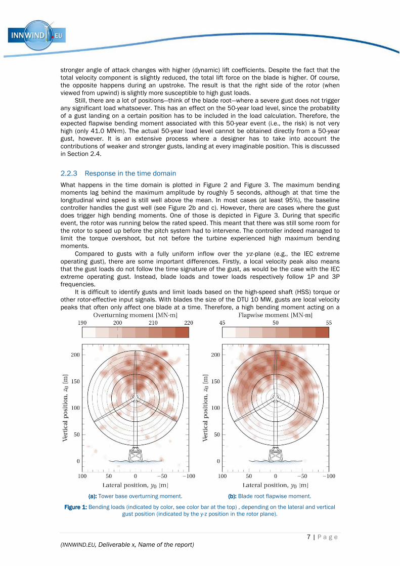
Figure 1 shows the tower overturning and blade flapwise bending moments as a function of the

gust landing on a range of �- and -positions. In both cases, the upper half of the rotor disk is the most vulnerable part, which is due to the wind shear profile. When added to the gust velocity, it causes high apparent wind speeds and higher angles of attack near the zero azimuth position. For the tower overturning moment, the gusts landing higher up have an even bigger impact due to the longer arm with respect to the tower base.

In addition, there is also some asymmetry in the lateral plane. We investigated this by feeding the mean gust shape to a simplified, fixed speed, fixed pitch model of the DTU 10 MW rotor. This mean gust shape is retrieved from the expected value of Equation (2.5) of the D1.12 report; that is,

�� ∗��∗��. (2.1)

Using the rotationally sampled velocity signals, we found that the asymmetry is caused by the correlation tensor prescribed by the Mann model. Positive streamwise amplitudes are often accompanied by negative (downward) vertical velocities. Therefore, a blade hit by a gust during its downstroke will also experience a decrease in the azimuthal velocity component. This causes


stronger angle of attack changes with higher (dynamic) lift coefficients. Despite the fact that the total velocity component is slightly reduced, the total lift force on the blade is higher. Of course, the opposite happens during an upstroke. The result is that the right side of the rotor (when viewed from upwind) is slightly more susceptible to high gust loads.

Still, there are a lot of positions—think of the blade root—where a severe gust does not trigger any significant load whatsoever. This has an effect on the 50-year load level, since the probability of a gust landing on a certain position has to be included in the load calculation. Therefore, the expected flapwise bending moment associated with this 50-year event (i.e., the risk) is not very high (only 41.0 MN·m). The actual 50-year load level cannot be obtained directly from a 50-year gust, however. It is an extensive process where a designer has to take into account the contributions of weaker and stronger gusts, landing at every imaginable position. This is discussed in Section 2.4.

2.2.3 Response in the time domain

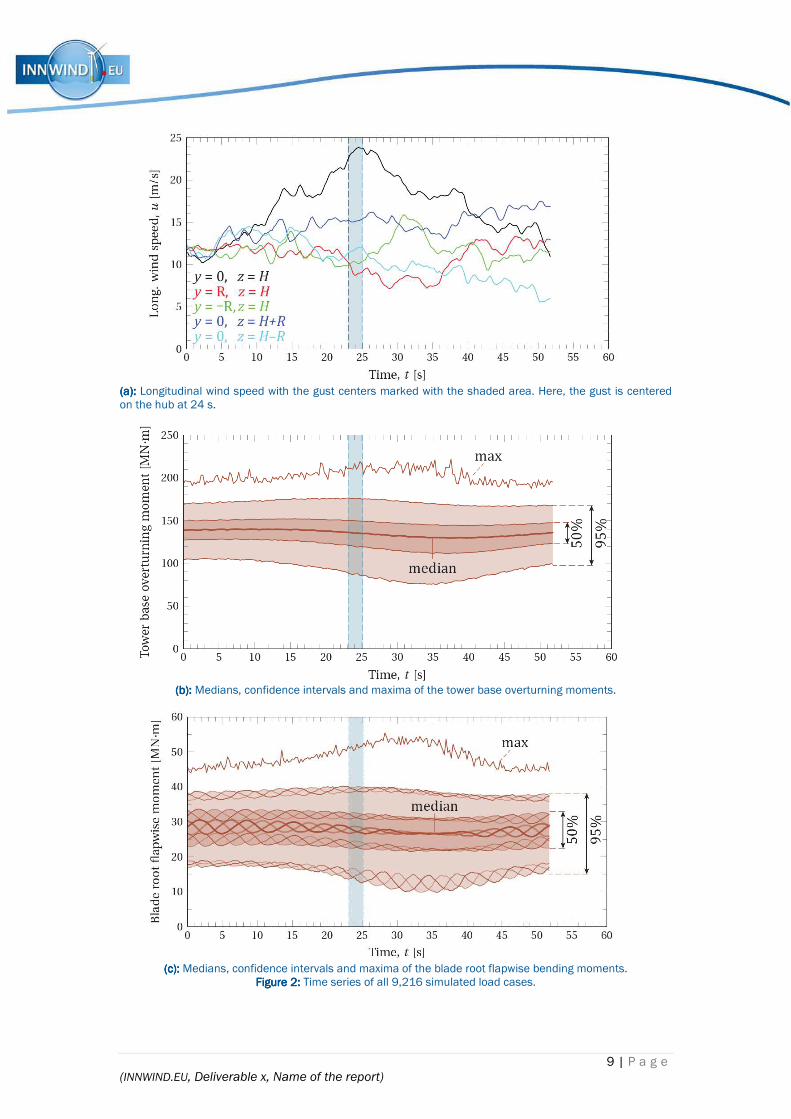
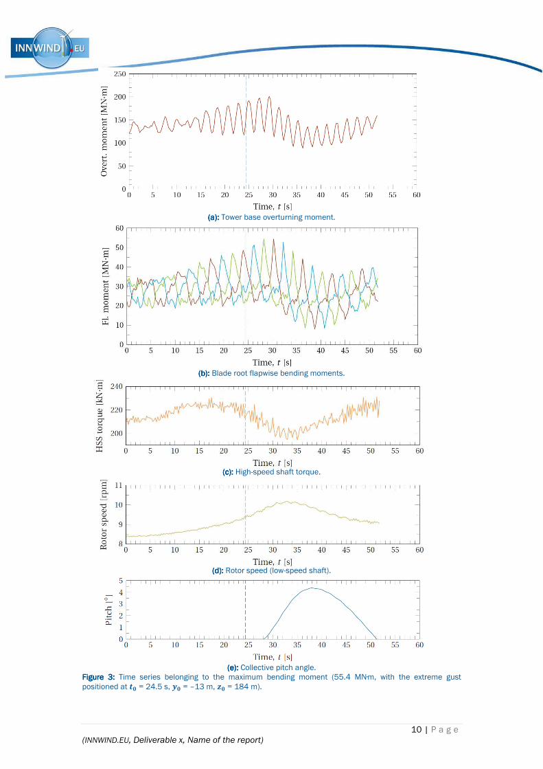
What happens in the time domain is plotted in Figure 2 and Figure 3. The maximum bending moments lag behind the maximum amplitude by roughly 5 seconds, although at that time the longitudinal wind speed is still well above the mean. In most cases (at least 95%), the baseline controller handles the gust well (see Figure 2b and c). However, there are cases where the gust does trigger high bending moments. One of those is depicted in Figure 3. During that specific event, the rotor was running below the rated speed. This meant that there was still some room for the rotor to speed up before the pitch system had to intervene. The controller indeed managed to limit the torque overshoot, but not before the turbine experienced high maximum bending moments.

Compared to gusts with a fully uniform inflow over the � -plane (e.g., the IEC extreme operating gust), there are some important differences. Firstly, a local velocity peak also means that the gust loads do not follow the time signature of the gust, as would be the case with the IEC extreme operating gust. Instead, blade loads and tower loads respectively follow 1P and 3P frequencies.

It is difficult to identify gusts and limit loads based on the high-speed shaft (HSS) torque or other rotor-effective input signals. With blades the size of the DTU 10 MW, gusts are local velocity peaks that often only affect one blade at a time. Therefore, a high bending moment acting on a

((((aaaa): ): ): ): Tower base overturning moment. ((((bbbb): ): ): ): Blade root flapwise moment.

Figure Figure Figure Figure 1111: : : : Bending loads (indicated by color, see color bar at the top) , depending on the lateral and vertical gust position (indicated by the y-z position in the rotor plane).


single blade root is not necessarily accompanied by high torque. For the same reason, high blade root moments do not always mean high tower moments.

Because the angle of attack changes are very local, collective pitch is a very crude measure and can lead to adverse results in the case of negative gust amplitudes. In the case of the NREL 5 MW machine with the baseline controller (see Figure 9), this turned out to be solely responsible for the 50-year load. A better solution is to rely on individual pitch, distributed control, and/or lidar-assisted control.


((((aaaa): ): ): ): Longitudinal wind speed with the gust centers marked with the shaded area. Here, the gust is centered on the hub at 24 s.

((((bbbb): ): ): ): Medians, confidence intervals and maxima of the tower base overturning moments.

((((cccc): ): ): ): Medians, confidence intervals and maxima of the blade root flapwise bending moments.

Figure Figure Figure Figure 2222: : : : Time series of all 9,216 simulated load cases.


((((aaaa): ): ): ): Tower base overturning moment.

((((bbbb): ): ): ): Blade root flapwise bending moments.

((((cccc): ): ): ): High-speed shaft torque.

((((dddd): ): ): ): Rotor speed (low-speed shaft).

((((eeee): ): ): ): Collective pitch angle.

Figure Figure Figure Figure 3333: : : : Time series belonging to the maximum bending moment (55.4 MN·m, with the extreme gust

positioned at �� = 24.5 s, �� = –13 m, �� = 184 m).


2.32.32.32.3 LidarLidarLidarLidar----assisted controlassisted controlassisted controlassisted control

Another interesting application is the reconstruction of lidar data. On the assumption that turbulence is a stationary, homogeneous, and Gaussian process, the statistics of any 3D spectral model can be used to give the best possible estimate for the velocity field. This was demonstrated using data from the LAWINE project (concluded in October 2016). More details of this method can be found in the paper (Bos et al., 2016).

2.3.1 Set-up

The set-up consisted of an Avent-Lidar 5-beam pulsed lidar prototype that was mounted on the nacelle of a Darwind XD115-5MW wind turbine on the test site of ECN (see Figure 4). It provides data of ten range gates simulatenously (50—185 m upwind), while cycling between the five beam positions (0—4) every 0.25 s.

The lidar does not provide a perfect point measurement, but more of a weighted average. This is modeled by a Gaussian pulse shape (Frehlich et al., 2006):

�� 12Δ� �erf #� − � + �&Δ�Δ' ( − erf #� − � − �&Δ�Δ' () (2.2)

where � is the distance to the range gate, Δ� the distance between the range gates, Δ' the e��

radius of the pulse, and erf�* is the error function. The e�� radius is derived from the full-width-at-half-maximum pulse width (FWHM):

Δ' � FWHM2√ln 2, (2.3)

with FWHM � 30 m for this set-up. Under the assumption that the streamwise velocity component

is the dominant one (i.e., 3 ≫ 5,�), the line-of-sight velocity at a given point 6 is:

3789,: � cos>: ?3@*: + �, �: , :A��d�, (2.4)

where > is the beam angle.

2.3.2 Velocity field reconstruction

The 3D velocity field that surrounds the collection of C measurements is a conditional field:

DE�F � GD�F|?3�*� + �, �� , ��d� � 3789,�cos>� , … ,?3�*J + �, �J, J��d� � 3789,Jcos>JK. (2.5)

Using the theory of D1.12, it is possible to derive the set of velocity fields that match the set of measurements, while adhering to the statistics of the spectral tensor, L�M. For this, we assume

that D�F is stationary, homogeneous, and Gaussian and can be constructed by a Fourier series:

Figure Figure Figure Figure 4444: : : : Sketch of the pulsed lidar system mounted on the nacelle of a Darwind XD115-5MW wind turbine.


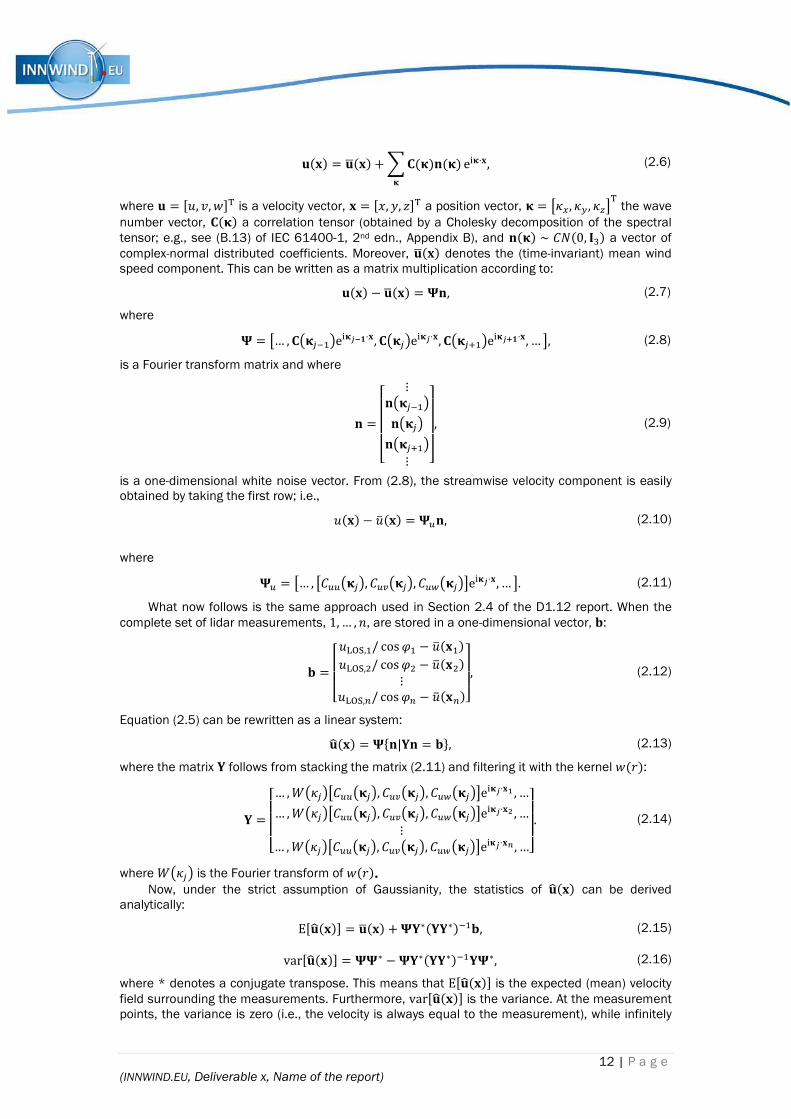
D�F � D��F +NO�M��MM

ePM⋅F, (2.6)

where D � R3, 5, �ST is a velocity vector, F � R*, �, ST a position vector, M � UVW, VX , VYZT the wave

number vector, O�M a correlation tensor (obtained by a Cholesky decomposition of the spectral tensor; e.g., see (B.13) of IEC 61400-1, 2nd edn., Appendix B), and ��M ∼ \]�0, _` a vector of

complex-normal distributed coefficients. Moreover, D��F denotes the (time-invariant) mean wind speed component. This can be written as a matrix multiplication according to:

D�F − D��F � a�, (2.7)

where

a � U… , O@M:��AePMbcd⋅F, O@M:AePMb⋅F, O@M:e�AePMbfd⋅F, … Z, (2.8)

is a Fourier transform matrix and where

� �ghhhhi ⋮�@M:��A�@M:A�@M:e�A⋮ kl

lllm, (2.9)

is a one-dimensional white noise vector. From (2.8), the streamwise velocity component is easily obtained by taking the first row; i.e.,

3�F − 3n�F � ao�, (2.10)

where

ao � U… , U\oo@M:A, \op@M:A, \oq@M:AZePMb⋅F, … Z. (2.11)

What now follows is the same approach used in Section 2.4 of the D1.12 report. When the

complete set of lidar measurements, 1,… , C, are stored in a one-dimensional vector, �:

� �ghhi3789,�/ cos >� − 3n�F�3789,&/ cos >& − 3n�F&⋮3789,J/ cos >J − 3n�FJkl

lm, (2.12)

Equation (2.5) can be rewritten as a linear system:

DE�F � ar�|s� � �t, (2.13)

where the matrix s follows from stacking the matrix (2.11) and filtering it with the kernel ��: s �

ghhhi… ,u@V:AU\oo@M:A, \op@M:A, \oq@M:AZePMb⋅Fv , …… ,u@V:AU\oo@M:A, \op@M:A, \oq@M:AZePMb⋅Fw , …⋮… ,u@V:AU\oo@M:A, \op@M:A, \oq@M:AZePMb⋅Fx , …kl

llm. (2.14)

where u@V:A is the Fourier transform of ��. . . .

Now, under the strict assumption of Gaussianity, the statistics of DE�F can be derived analytically:

ERDE�FS � D��F + as∗�ss∗��, (2.15)

varRDE�FS � aa∗ −as∗�ss∗��sa∗, (2.16)

where * denotes a conjugate transpose. This means that ERDE�FS is the expected (mean) velocity

field surrounding the measurements. Furthermore, varRDE�FS is the variance. At the measurement points, the variance is zero (i.e., the velocity is always equal to the measurement), while infinitely


far away, the variance should be equal to the square of the turbulence intensity (i.e., the best guess with only the ten-minute statistics). The process can be best compared to kriging—which was originally applied in geostatistics—where the variance is representative of the uncertainty.

2.3.3 A gust measured in the field

This method was applied to a gust that was picked up by the lidar’s center beam on 22 December 2013. It was the most severe event in the 1.5-year data set, while still being undisturbed from the surrounding turbines and met masts.

Assuming that the terrain is relatively flat and homogeneous, a neutral wind shear profile was fitted to the ten-minute mean wind speeds measured at the positions 0, 1 and 3 at � � -140 m:

3n� � 3n� |}~ ln� / �ln� / |}~, (2.17)

which resulted in a roughness length of � � 0.55 m, matching the site fairly well (de Jong et al.,

1990). In addition, Mann’s spectral tensor was set up with � ≈ 25 m (estimated from the low-frequency part of the lidar spectrum), Γ � 3 (for neutral conditions) (Sathe et al., 2013), and ��&/` ≈ 0.16 m4/3/s2. The latter was found by matching the longitudinal variance of the center beam measurements to the filtered spectral tensor:

?u&�VWΦoo�MdV ≈ �o,789& , (2.18)

Figure 5 shows two cross-sections of the fields ERDE�FS and varRDE�FS. The low-frequency parts of the gust, which hold most of the momentum content, are captured fairly well. The variance is the lowest along the directions of the beams, as should be expected. However, it never reaches complete zero due to the range weighting, so part of this variance has to account for the high frequencies that are not captured by the lidar.

Figure Figure Figure Figure 5555: : : : Expected velocity fields in the yz- (aaaa) and xz-planes (bbbb), together with the normalized variance in the yz- (cccc) and xz-planes (dddd).


2.3.4 Construction of a control input signal

The expected velocity field, together with its variance, can be used to construct an input signal for a gust controller. It relies on the notion that, under Taylor’s frozen turbulence hypothesis, it holds that

�3n �3�* � −��*,

��* ��3n3 + � � 0,

�3n3 + � � const. (2.19)

Here, � is the air density and � is the static atmospheric pressure. The along-wind force, pushing

on the � -plane at a distance � upwind, is found by integrating the dynamic pressure term, �3n3, over a surface, �:

��; � � ��3n��, �, 3��, �, , �d�d �

. (2.20)

Because 3n�F is constant and 3�F, � is a Gaussian field, it must follow that ��; � is also Gaussian. This is convenient, since it allows us to also derive its statistics, based on the statistics of a reconstructed velocity field, 3��F, �: EU��; �Z � ��3n��, �, ER3��, �, , �Sd�d

�, (2.21)

varU��; �Z � �&��3n&��, �, varR3��, �, , �Sd�d �

. (2.22)

This along-wind force is related to the loads on the structure and can be used for gust

control. For example, with 97.7% certainty, the along-wind force will stay under the level �� + 2�� (see Figure 6). The uncertainty is a function of the turbulence coherence and the amount of available measurement points, which will vary due to the technical availability of the lidar and the

blades passing in front of the eye. Therefore, a signal �� + C�� is a rather objective way of judging the lidar input.

The method was cross-checked with a similar input signal: the rotor-effective wind speed, �}~~, which is a pseudo-signal that is directly derived from the measured rotor torque:

� � ��\��, ��`�}~~& , (2.23)

where � is the shaft torque, \� the torque coefficient (a function of the pitch angle, �, and tip

speed ratio, �), and � the rotor diameter. The rotor-effective wind speed has been proven to be a good input signal for feed-forward control and has been successfully implemented to improve turbine behavior under gust loading (van der Hooft et al., 2003, 2004). Figure 7 shows a direct comparison of the two signals by matching their mains. The rotor-effective wind speed was downsampled to 1 Hz (was 64 Hz) to reduce the noise and focus on the more important low-

frequency fluctuations. The 95% range follows from the area enclosed by �� ± 2��. The two signals seem to agree well in a qualitative sense, with the most important up- and downward trends

around � � 0 clearly recognizable.


2.42.42.42.4 DLC 1.1 DLC 1.1 DLC 1.1 DLC 1.1 extreme load predictionsextreme load predictionsextreme load predictionsextreme load predictions

Probably the most powerful application of constrained stochastic simulation is in the prediction of extreme loads. Extreme loads, most notably the 50-year loads, are difficult to obtain because certain dynamic behavior or controller behavior might only show up in very large sample sizes. This often makes it hard to model the extreme load behavior in cases when the computational budget is limited; for example, in early design phases.

2.4.1 Case study: the NREL 5 MW

As a case study, we considered the NREL 5 MW. This was a convenient subject, since a large data set was available with 96 years’ worth of extremes (Barone et al., 2013).1 At the same time, it provided a nice insight in the controller behavior in extreme cases. The data set was generated

1 Downloadable from http://energy.sandia.gov/?page_id=13173.

Figure Figure Figure Figure 6666: : : : Expected along-wind force belonging to the gust event of Figure 5 at � � –140 m, together with the uncertainty levels.

Figure Figure Figure Figure 7777: : : : Expected along-wind force belonging to the gust event of Figure 5 at � � –140 m, compared to the rotor-effective wind speed by ECN with a 10.5-s delay to account for advection towards the rotor disk (downsampled to 1 Hz for clarity).


using the onshore version of the NREL 5 MW with the baseline controller, modeled in FAST v7. Wind fields were generated by TurbSim on a 137×137 m, 20×20 grid, with a temporal frequency of 20 Hz, and following an IEC class 1B normal turbulence model. Each simulation was run for 11 minutes, with the first minute discarded to get rid of the start-up transients.

The data set was generated by a crude Monte Carlo method. This means that the mean wind speeds were sampled from the parent Rayleigh distribution and that the extreme load distribution

follows naturally from sorting an assigning the appropriate plotting position to the �th load:

��@�X,�A � �] + 1, (2.24)

where ] is the sample size. The regions below the cut-in and above cut-out wind speeds can be accounted for by either completing the data set with zero loads or by correcting the load distribution according to

��@�X,�A � 1 − �1 − �] + 1 ? ¡��d��¢£¤�¥£¤¢£¤�P¦

. (2.25)

Figure 8 shows the extreme blade root flapwise bending moments. Judging from both the scatter plot (a) and the return level plot (b), the extreme loads seem to originate from relatively high wind speeds in the pitch control regime. It turned out that this was due to a particular weakness in the baseline controller. Strongly negative gust amplitudes would sometimes reduce the wind speed close to the rated wind speed, which causes the turbine to pitch back to zero. When the wind speed recovers, the machine is operating at full thrust in an 18—19-m/s mean wind speed, leading to the high extreme loads (e.g., see Figure 9). When the data set increases in size, the extreme cases appear in even higher wind speeds, since increasingly larger amplitudes are encountered that are able to bring the wind speed back to rated. This also means that, for small sample sizes, the extremes might seem to lie close to the rated wind speed, which is also what is shown by the error bars in Figure 8a.

(a): (a): (a): (a): Scatter plot of the entire data set. The edges of the box plots indicate the 25th and 75th percentiles, the whiskers indicate the 2.5th and 97.5th percentiles, and the bar shows the medians.

(b): (b): (b): (b): Return level plot, yielding a 50-year extreme of 17.8 MN·m. Longer return periods are obtained by fitting a generalized extreme value distribution. The shaded area marks the 95% confidence interval, which is estimated by resampling the data.

Figure Figure Figure Figure 8888: : : : Extreme blade root flapwise moments of the NREL 5 MW reference turbine (§ � 5 · 106).


2.4.2 An importance sampling method

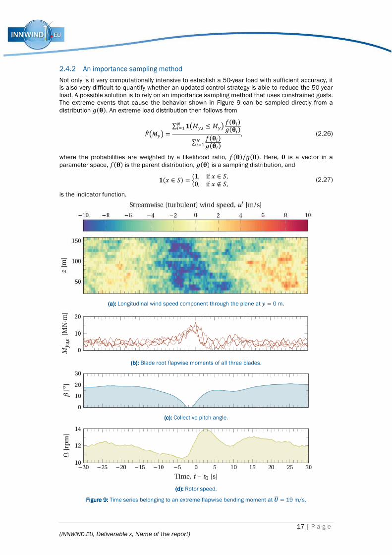
Not only is it very computationally intensive to establish a 50-year load with sufficient accuracy, it is also very difficult to quantify whether an updated control strategy is able to reduce the 50-year load. A possible solution is to rely on an importance sampling method that uses constrained gusts. The extreme events that cause the behavior shown in Figure 9 can be sampled directly from a

distribution ¨�©. An extreme load distribution then follows from

��@�XA � ∑ d@�X,� ≤ �XA ¡�©�¨�©�¬��∑ ¡�©�¨�©�¬��

, (2.26)

where the probabilities are weighted by a likelihood ratio, ¡�©/¨�©. Here, © is a vector in a

parameter space, ¡�© is the parent distribution, ¨�© is a sampling distribution, and

d�* ∈ ¯ � G1, if* ∈ ¯,0, if* ∉ ¯, (2.27)

is the indicator function.

(a): (a): (a): (a): Longitudinal wind speed component through the plane at � � 0 m.

((((bbbb): ): ): ): Blade root flapwise moments of all three blades.

((((cccc): ): ): ): Collective pitch angle.

((((dddd): ): ): ): Rotor speed.

Figure Figure Figure Figure 9999: : : : Time series belonging to an extreme flapwise bending moment at ²� � 19 m/s.


Importance sampling can be a very attractive solution when a designer has complete control over the wind field. Instead of running large sample sizes of ten-minute wind fields, the same results can be obtained by only evaluating the response to a small set of extreme gusts, which can be stored in time series of 1—2 minutes.

The critical part of an importance sampling method is always to define a proper sampling distribution. We assume that the extremes loads are dependent on 2 parameters: the mean wind

speed, ��, and the gust amplitude, �. The gust position is left unconstrained (i.e., uniformly

distributed over the � -plane). Then, an initial survey of the parameter space, shown in Figure 10, explains the scatter of Figure 8a. It confirms the suspicion that combinations of high wind speeds and large negative gust amplitudes are responsible for the extreme load behavior.

The probability associated with such gusts are estimated through the Euler characteristic heuristic:

¡�� ≈ − dd� ER>�'�S, (2.28)

where the expected Euler characteristic, ER>�'�S, is given by Equation (3.13) of the D1.12 report. Based on Figure 10, two different gust settings are used: (1) a point gust (i.e., exciting a single grid point) and (2) a spheroidal gust with a time scale of 2 s and a lateral diameter of 25 m. The 50-year amplitudes for these events lie approximately at the ±8� and ±7� level, respectively. Two sampling distributions are then set up:

¨��, � ≈ 12π ⋅ 2 ⋅ 0.5 exp �− �� − 20&2 ⋅ 2& − �� ⁄ + 7&2 ⋅ 0.5& ), (2.29)

Figure Figure Figure Figure 10101010: : : : Extreme blade root flapwise moments of the NREL 5 MW reference turbine triggered by point gust

amplitudes (§ � 105).


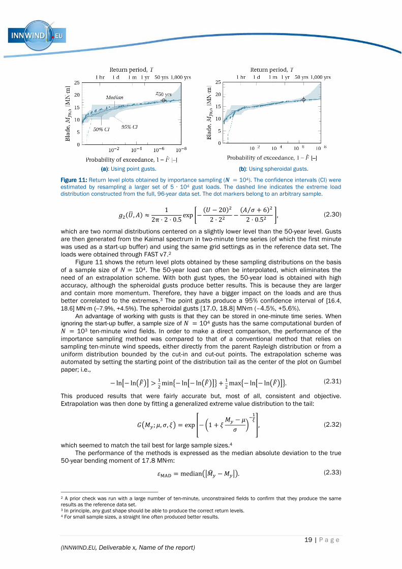
¨&��, � ≈ 12π ⋅ 2 ⋅ 0.5 exp �− �� − 20&2 ⋅ 2& − �� ⁄ + 6&2 ⋅ 0.5& ), (2.30)

which are two normal distributions centered on a slightly lower level than the 50-year level. Gusts are then generated from the Kaimal spectrum in two-minute time series (of which the first minute was used as a start-up buffer) and using the same grid settings as in the reference data set. The loads were obtained through FAST v7.2

Figure 11 shows the return level plots obtained by these sampling distributions on the basis of a sample size of ] � 104. The 50-year load can often be interpolated, which eliminates the need of an extrapolation scheme. With both gust types, the 50-year load is obtained with high accuracy, although the spheroidal gusts produce better results. This is because they are larger and contain more momentum. Therefore, they have a bigger impact on the loads and are thus better correlated to the extremes.3 The point gusts produce a 95% confidence interval of [16.4, 18.6] MN·m (–7.9%, +4.5%). The spheroidal gusts [17.0, 18.8] MN·m (–4.5%, +5.6%).

An advantage of working with gusts is that they can be stored in one-minute time series. When ignoring the start-up buffer, a sample size of ] � 104 gusts has the same computational burden of ] � 103 ten-minute wind fields. In order to make a direct comparison, the performance of the importance sampling method was compared to that of a conventional method that relies on sampling ten-minute wind speeds, either directly from the parent Rayleigh distribution or from a uniform distribution bounded by the cut-in and cut-out points. The extrapolation scheme was automated by setting the starting point of the distribution tail as the center of the plot on Gumbel paper; i.e.,

− lnU− ln@��AZ > �&min¼− lnU− ln@��AZ½ + �&max¼− lnU− ln@��AZ½. (2.31)

This produced results that were fairly accurate but, most of all, consistent and objective. Extrapolation was then done by fitting a generalized extreme value distribution to the tail:

¾@�X; ¿, �, ÀA � exp Á− �1 + À�X − ¿� ��ÂÃ, (2.32)

which seemed to match the tail best for large sample sizes.4 The performance of the methods is expressed as the median absolute deviation to the true

50-year bending moment of 17.8 MN·m:

ÄÅÆÇ � median@È�ÉX −�XÈA. (2.33)

2 A prior check was run with a large number of ten-minute, unconstrained fields to confirm that they produce the same results as the reference data set. 3 In principle, any gust shape should be able to produce the correct return levels. 4 For small sample sizes, a straight line often produced better results.

(a)(a)(a)(a): Using point gusts. ((((bbbb)))): Using spheroidal gusts.

Figure Figure Figure Figure 11111111: : : : Return level plots obtained by importance sampling (§ � 104). The confidence intervals (CI) were estimated by resampling a larger set of 5 · 104 gust loads. The dashed line indicates the extreme load distribution constructed from the full, 96-year data set. The dot markers belong to an arbitrary sample.


This is similar to the root-mean-squared error, but is less distorted by extremely bad fits. Figure 12 then shows the comparison of the methods. For the same quality result, the importance sampling method is, in general, about two orders of magnitude faster than sampling ten-minute mean wind speeds. This makes it especially suitable for early design phases when computational resources are scarce.

2.52.52.52.5 ReferencesReferencesReferencesReferences

Barone, M., Paquette, J., Resor, B., and Manuel, L. (2012). Decades of wind turbine load simulation, 50th AIAA Aerosp. Sci. Meet. Incl. New Horizons Forum Aerosp. Expo., Nashville, TN, United States, 9–12 January, 2012, doi:10.2514/6.2012-1288.

Bos R, Giyanani A, Bierbooms W. (2016). Assessing the severity of wind gusts with lidar. Remote Sens, 8, 758. doi:10.3390/rs8090758.

Frehlich, R.; Meillier, Y.; Jensen, M.L.; Balsley, B.; Sharman, R. (2006). Measurements of boundary layer profiles in an urban environment. J. Appl. Meteorol. Climatol, 45, 821—837.

van der Hooft, E.L.; Schaak, P.; van Engelen, T.G. (2003). Wind Turbine Control Algorithms, Energy Research Centre of The Netherlands: Petten, The Netherlands.

van der Hooft, E.L.; van Engelen, T.G. (2004). Estimated wind speed feed forward control. In: Proceedings of the European Wind Energy Conference, 22—25 November 2004,London, UK.

de Jong, J.J.M.; de Vries, A.C.; Klaasen, W. (1990). Influence of obstacles on the aerodynamic roughness of the Netherlands. Bound Lay. Meteorol., 91, 51—64.

Sathe, A.R.; Mann, J.; Barlas, T.; Bierbooms, W.A.A.M.; van Bussel, G.J.W. (2013). Influence of atmospheric stability on wind turbine loads. Wind Energy, 16, 1013—1032.

Figure Figure Figure Figure 12121212: : : : Median-absolute deviation to the 50-year load as obtained by the importance sampling method (IS), compared to sampling ten-minute mean wind speeds from a uniform distribution and from the parent Rayleigh distribution (i.e., crude Monte Carlo).


CHAPTER CHAPTER CHAPTER CHAPTER 1111 3

3.13.13.13.1 First paragraphFirst paragraphFirst paragraphFirst paragraph

3.1.1 Second paragraph


CHAPTER CHAPTER CHAPTER CHAPTER 2222 4


CHAPTER 3CHAPTER 3CHAPTER 3CHAPTER 3 5

5.15.15.15.1 First ParagraphFirst ParagraphFirst ParagraphFirst Paragraph

5.1.1 xxxx


Appendix A


Table Table 1.

Date

Meeting Location

March 2014 Progress meeting 3 TBD

Table 2.

Table 3.

applications of constrained stochastic simulation … · the mean gust shape to a simplified, fixed...

Documents