applications of calculus i – book from your calculus text along with a detailed solution. ......
TRANSCRIPT


Preface
One of the goals of the EXCEL program is to enhance understanding of mathematics (primarily calculus) for Science, Technology, Engineering and Mathematics (STEM) students. Mathematics is considered the cornerstone of the success of any student pursuing a degree in a STEM discipline. One way of achieving this goal at UCF is by introducing students to the Applications of Calculus courses. This book is the textbook material for the Applications of Calculus II course that you will be taking in the spring semester of your freshman studies at UCF. It is comprised of a series of chapters written by EXCEL faculty from various disciplines of the sciences, engineering and mathematics. These chapters and the presentations that the individual EXCEL faculty members will make in the Applications of Calculus II class will show you how material that you will be learning in your Calculus II class is actually used in the discipline of the faculty presenter. These presentations are correlated with the sections of your calculus book and will be presented just shortly after you cover those sections in your Calculus II class.
Each of the chapters of this book is organized in the same way. The chapters begin with a section titled Calculus Topic which includes at least one calculus problem taken directly from your calculus text along with a detailed solution. The purpose of including a problem from your calculus text is to 1) reinforce the techniques used to solve problems from that particular section and 2) to explain how a particular mathematical concept is related to a particular physical (real world) problem. The next section in each chapter is a Background/Motivation section. This section provides you with the basic understanding of the field of study that will follow and why the mathematics (in particular, a Calculus II topic) is necessary in that field of study. Following the Background/Motivation section you will find a series of Learning Objectives. Each Learning Objective is followed by text, figures and tables which lead the reader through the process of understanding that objective. Each of the Learning Objectives shown in a chapter will be a focus of the faculty presentation. The faculty presenters are outstanding educators and researchers in their respective fields. Each faculty member authored his/her chapter as well as the presentation that will be given in class.
We hope that you, the reader and student, find this book to be helpful in your journey through this course, that the course offers a useful enhancement to your understanding of Calculus and that the weekly presentations broaden your horizons and peek your interests in topics of mathematics, engineering and sciences that you may have never otherwise studied on your own.
Acknowledgements
First and foremost, we would like to acknowledge the support of the National Science Foundation grant DUE 05254209, who has entrusted us with the opportunity to educate the STEM youth of tomorrow.
We also want to acknowledge the generous support from Provost Hickey, Vice–Provost Schell, the UCF Office of Research and Commercialization (in particular, the Vice–President of Research Dr. Soileau), the College of Engineering and Computer Science Dean’s Office (in particular, Dean Gallagher, Associate Dean Nayfeh and Ms. Falls), the College of Sciences Dean’s Office (in particular, Dean Panousis, Associate Dean Johnson and Ms. Kirkpatrick), the Office of Operational Excellence and Assessments (in particular, Drs. Pet–Armacost, Krist and Lancey), the Institutional Research Office (in particular, Ms. Ramsey), UCF Admissions Office (in particular, Dr. Chavis and Ms. Costello), the First Year Advising Office (in particular, Ms. Priest and Ms. Datta), the UCF Orientation Office (in particular, Mr. Richie and Mr. Hicks), the UCF Diversity Office (in particular, Dr. King), the UCF Housing Office (in particular, Mr. Paulick, Mr. Novak and Ms. Rutkowski) and Associate Provost Poisel, amongst many others.
This book would not have been possible without the hard work and dedication of the EXCEL faculty: Drs. Georgiopoulos and Young (EXCEL Directors), who have been involved with all aspects of this project from planning, writing, coordinating, scheduling to the more thankless jobs of handling the finances of the project. Drs. Geiger, Hagen, Islas and Winningham (EXCEL Coordinators), all of which spent a tremendous amount of time in planning and directing this project as well as their continuing projects. The EXCEL faculty who have contributed their knowledge and expertise in order to make this book a reality are Drs. Kocak (Chapter 1), Ou (Chapter 2), Rollins (Chapters 3 and 5), da Vitoria Lobo (Chapter 4), Efthimiou (Chapter 6) and Turgut (Chapter 7). The assessment and evaluation materials associated with this class were developed by the Faculty Center for Teaching and Learning under the guidance of Drs. Morisson–Shetlar and Crouse, and this is a contribution for which we are very thankful. Special thanks go to the EXCEL graduate students: Peter Bacopoulos, Erin Holland, Chris Sentelle, Todd Smith and Tomasz Wlodarczyk, who reviewed and critiqued every chapter in this book. These students gave their time and energy to review all the chapters in this book and provided excellent advice to the EXCEL faculty in changing the chapter write–up to enhance its understandability by the EXCEL students.
Finally, the load of integrating the information from seven different EXCEL faculty into a cohesive volume of work fell upon Tomasz Wlodarczyk and Peter Bacopoulos, who did an outstanding job under the guidance of the EXCEL coordinator, Dr. Hagen. We are very grateful for their effort.

Table of Contents
1 Sigmoid functions and their usage in artificial neural networks.......................................... 1–1 2 Laplace Transforms and initial value problems................................................................... 2–1 3 Mathematical Modeling of the Population Growth of a Single Species I – Continuous..... 3–1 4 Interactive Graphics Curves using Parametric Equations.................................................... 4–1 5 Mathematical Modeling of the Population Growth of a Single Species II – Discrete......... 5–1 6 The Geometric Series and Some Applications .................................................................... 6–1 7 Multipath Effects in Wireless Networks.............................................................................. 7–1

Chapter 1
1 Sigmoid functions and their usage in artificial neural networks by Dr. Taskin Kocak Weeks: 1/8 and 1/15 of Spring 2007
Sigmoid functions and their usage in artificial neural networks 1–2
Calculus Topic: Hyperbolic Functions Section 7.6 #19: Prove identity
xexx 2
tanh1tanh1
=−+
2
21
2
21
coshsinh1
coshsinh1
tanh1tanh1
xx
xx
xx
xx
ee
ee
ee
ee
xxxx
xx
−
−
−
−
+
−
−
+
−
+
=−
+=
−+
xx
x
xx
xxxx
xx
xxxx
xx
xx
xx
xx
eee
eeeeee
eeeeee
eeeeeeee
2
22
1
1==
+
+−++
−++
=
+
−−
+
−+
=−
−
−−
−
−−
−
−
−
−
In this section we will discuss sigmoid functions, which belong to the family of
hyperbolic functions. We will also present their usage in artificial neural networks.
Background/Motivation A sigmoid function is a mathematical function that produces a sigmoid curve, i.e. a curve having an “S” shape. An example sigmoid function, which is the special case of the logistic function, is given below and it is plotted in Figure 1. A logistic function models the growth of some set. The initial stage of growth is approximately exponential; then growth slows and at maturity, growth stops.
tet
−+=
1
1)(sig (1)

Sigmoid functions and their usage in artificial neural networks 1–3
–6 –4 –2 0 2 4 6 0
0.1
0.2
0.3
0.4
0.5
0.6
0.7
0.8
0.9
1
Figure 1: Sigmoid function.
In general, a sigmoid function is real–valued and differentiable, having a non–negative or non–positive first derivative, one local minimum, and one local maximum. The logistic sigmoid function is related to the hyperbolic tangent as follows
2tanh
1121 xe x
−=+
−− (2)
Sigmoid functions are often used in artificial neural networks to introduce nonlinearity in the model. A neural network element computes a linear combination of its input signals, and applies a sigmoid function to the result. A reason for its popularity in neural networks is because the sigmoid function satisfies a property between the derivative and itself such that it is computationally easy to perform. Derivatives of the sigmoid function are usually employed in learning algorithms.
))(sig1)((sig)(sig tttdtd
−= (3)

Sigmoid functions and their usage in artificial neural networks 1–4
Learning objective #1: Determine the relationships between the biological and artificial neural networks Modern digital computers perform better than humans when it comes to numeric computation and related symbol manipulation. However, humans can beat the world’s fastest computer in solving complex perceptual problems such as recognizing a man in a crowd from a mere glimpse of his face at a high speed. The remarkable difference in their performance is due to the biological neural system architecture, which is completely different from the computer architecture.
A neuron (or nerve cell) is a special biological cell that processes information (see Figure 2). It is composed of a cell body, or soma, and two types of out–reaching tree–like branches: the axon and the dendrites. The cell body has a nucleus that contains information. A neuron receives signals (impulses) from other neurons through its dendrites (receivers) and transmits signals generated by its cell body along the axon (transmitter).
Figure 2: A sketch of a biological neuron.
Inspired by biological neural networks, Artificial Neural Networks (ANNs) are massive parallel computing systems consisting of an extremely large number of simple processors with many interconnections. McCulloch and Pitts [1] proposed a binary threshold unit as a computational model for an artificial neuron (see Figure 3).
Sigmoid functions and their usage in artificial neural networks 1–5
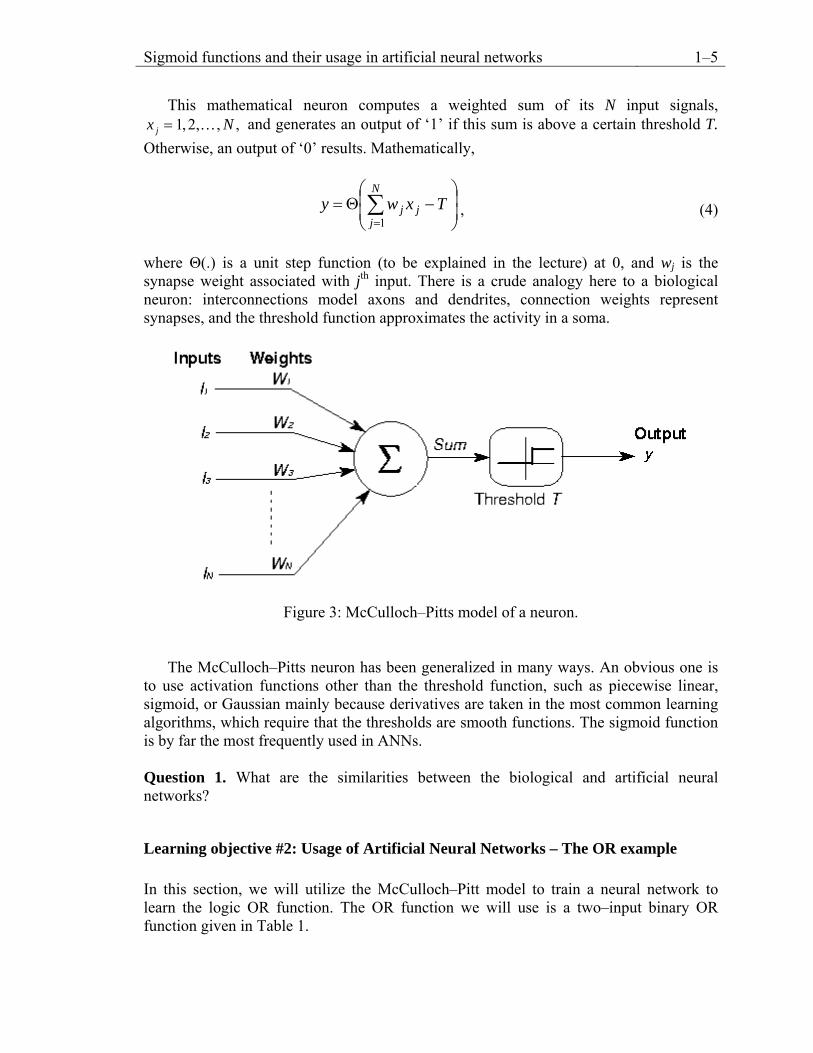
This mathematical neuron computes a weighted sum of its N input signals, 1,2, , ,jx N= K and generates an output of ‘1’ if this sum is above a certain threshold T.
Otherwise, an output of ‘0’ results. Mathematically,
⎟⎟⎠
⎞⎜⎜⎝
⎛−Θ= ∑
=
N
jjj Txwy
1, (4)
where Θ(.) is a unit step function (to be explained in the lecture) at 0, and wj is the synapse weight associated with jth input. There is a crude analogy here to a biological neuron: interconnections model axons and dendrites, connection weights represent synapses, and the threshold function approximates the activity in a soma.
Figure 3: McCulloch–Pitts model of a neuron.
The McCulloch–Pitts neuron has been generalized in many ways. An obvious one is to use activation functions other than the threshold function, such as piecewise linear, sigmoid, or Gaussian mainly because derivatives are taken in the most common learning algorithms, which require that the thresholds are smooth functions. The sigmoid function is by far the most frequently used in ANNs. Question 1. What are the similarities between the biological and artificial neural networks?
Learning objective #2: Usage of Artificial Neural Networks – The OR example In this section, we will utilize the McCulloch–Pitt model to train a neural network to learn the logic OR function. The OR function we will use is a two–input binary OR function given in Table 1.

Sigmoid functions and their usage in artificial neural networks 1–6
I1 I2 Output 0 0 0 0 1 1 1 0 1 1 1 1
Table 1: OR function.
First, we will use one neuron with two inputs as illustrated in Figure 4. Note that the inputs are given equal weights by assigning the weights (w’s) to ‘1’. The threshold, T, is set to 0 in this example.
Figure 4: One neuron model for the OR function. We calculate the output as follows:
1) Compute the total weighted inputs
∑=
=2
1iii wIX (5)
X = I1 w1+I2 w2 = I1 1+I2 1 = I1+I2 (6)
2) Calculate the output using the logistic sigmoid activation function
XeO
−+=
11
(7)
Now, let’s try it for the inputs given in Table 1. For I1 = 0 and I2 = 0; X = 0,
5.011
11
10 =
+=
+=
eO (8)
For I1 = 0 and I2 = 1, and I1 = 1 and I2 = 0; X = 1,

Sigmoid functions and their usage in artificial neural networks 1–7
73.037.01
11
11 ≅
+=
+= −e
O (9)
For I1 = 1 and I2 = 1; X = 2,
88.014.01
11
12 ≅
+=
+= −e
O (10)
For all cases the results are correct assuming that 0.5 and below are considered as ‘0’ and above as ‘1’. Question 2. If the weights were 0.5 rather 1, will the network still function like OR? Question 3. In groups of two students, discuss whether the same network can be used to learn the AND function? (Hint: You may change the threshold (=0.5) if necessary.)
I1 I2 Output 0 0 0 0 1 0 1 0 0 1 1 1
Table 2: AND function.
Learning objective #3: The classic XOR problem If we use the same one–neuron model to learn the XOR (exclusive or) function, the model will fail. The XOR function is given in Table 2. The first three cases will produce correct results; however, the last case should also be considered as ‘1’, which is not correct.
I1 I2 Output 0 0 0 0 1 1 1 0 1 1 1 0
Table 3: XOR function.
The solution is to add a middle (hidden in ANN terminology) layer between the inputs and the output neuron as shown in Figure 5.

Sigmoid functions and their usage in artificial neural networks 1–8
Figure 5: ANN with the hidden neurons for the XOR problem (note that there will be a threshold function at the final output (O)).
Choose the weights w11=w12=w21=w22=1. Use a different sigmoid function, which is given with a certain threshold for each neuron:
)2.0(
)5.1(2
)5.0(1
11)(
11)(
11)(
−−
−−
−−
+=
+=
+=
xO
xH
xH
exsig
exsig
exsig
(11)
Confirm by calculating the neuron outputs for each possible input combinations that this neural network is indeed functioning like an XOR. (Hint: The output equal or below 0.5 is considered ‘0’, otherwise ‘1’)
Reference [1] W. S. McCulloch and W. Pitts, “A logical calculus of the ideas immanent in neurons activity,” Bull. Math. Biophys., vol. 5, pp. 115–133, 1943.

Chapter 2
2 Laplace Transforms and initial value problems by Dr. Miaojung Ou Weeks: 1/22 and 1/29 of Spring 2007
Laplace Transforms and initial value problems 2–2
Calculus topic: Integration by parts
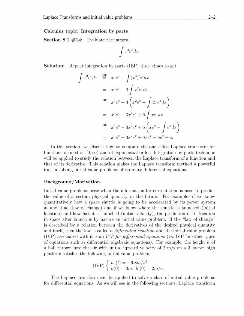
Section 8.1 #14: Evaluate the integral∫x3exdx.
Solution: Repeat integration by parts (IBP) three times to get∫x3exdx
IBP= x3ex −
∫(x3)′exdx
= x3ex − 3
∫x2exdx
IBP= x3ex − 3
(x2ex −
∫2xexdx
)
= x3ex − 3x2ex + 6
∫xexdx
IBP= x3ex − 3x2ex + 6
(xex −
∫exdx
)= x3ex − 3x2ex + 6xex − 6ex + c.
In this section, we discuss how to compute the one–sided Laplace transform forfunctions defined on [0,∞) and of exponential order. Integration by parts techniquewill be applied to study the relation between the Laplace transform of a function andthat of its derivative. This relation makes the Laplace transform method a powerfultool in solving initial value problems of ordinary differential equations.
Background/Motivation
Initial value problems arise when the information for current time is used to predictthe value of a certain physical quantity in the future. For example, if we knowquantitatively how a space shuttle is going to be accelerated by its power systemat any time (law of change) and if we know where the shuttle is launched (initiallocation) and how fast it is launched (initial velocity), the prediction of its locationin space after launch is by nature an initial value problem. If the “law of change”is described by a relation between the derivatives of the desired physical quantityand itself, then the law is called a differential equation and the initial value problem(IVP) associated with it is an IVP for differential equations (vs. IVP for other typesof equations such as differential–algebraic equations). For example, the height h ofa ball thrown into the air with initial upward velocity of 2 m/s on a 3–meter–highplatform satisfies the following initial value problem:
(IVP)
{h′′(t) = −9.8m/s2,h(0) = 3m, h′(0) = 2m/s.
The Laplace transform can be applied to solve a class of initial value problemsfor differential equations. As we will see in the following sections, Laplace transform

Laplace Transforms and initial value problems 2–3
provides a powerful tool to rewrite the differential equation together with the ini-tial conditions as one algebraic equation through integration by parts. The solution(prediction) is then obtained by solving the algebraic equation followed by inverseLaplace transform.
Learning Objective #1: Calculation of Laplace transform of elementaryfunctions
Definition 1. The one–sided Laplace transform of a function f defined on [0,∞) isa function of s such that
L{f}(s) :=
∫ ∞
0
e−stf(t)dt.
The domain of L{f} is where the integral exists.
Example 1. Calculate the Laplace transform of f(t) = 1.
L{1}(s) :=
∫ ∞
0
e−st · 1dt
:= limN→∞
∫ N
0
e−stdt
= limN→∞
e−st
−s
∣∣∣∣t=N
t=0
= limN→∞
(e−sN
−s− 1
−s
)=
1
s.
So the Laplace transform of the constant function f(t) = 1 is1
sfor s > 0.
Example 2. Calculate the Laplace transform of f(t) = t.
L{t}(s) :=
∫ ∞
0
e−st · tdt
:= limN→∞
∫ N
0
te−stdt
IBP= lim
N→∞
[te−st
−s
∣∣∣∣t=N
t=0
−∫ N
0
e−st
−sdt
]
= limN→∞
(Ne−sN
−s− e−sN
s2+
1
s2
)
=1
s2for s > 0.
Note that L’Hospital Rule was applied to evaluate the first term in the limit.

Laplace Transforms and initial value problems 2–4
Question 1. Use similar ideas to calculate the Laplace transform of f(t) = t2. Doyou identify some pattern? Use the pattern to make your best guess on L{tn} forn = 3.What about for n = 10?
Example 3. Calculate the Laplace transform of f(t) = sin t.
L{sin t}(s) :=
∫ ∞
0
e−st · sin tdt
:= limN→∞
∫ N
0
e−st sin tdt.
We evaluate
∫ N
0
e−st sin tdt by using integration by parts as follows:
∫ N
0
e−st sin tdtIBP=
e−st · sin t
−s
∣∣∣∣t=N
t=0
−∫ N
0
e−st · cos t
−sdt
=
(e−sN · sin N
−s− 0
)+
1
s
∫ N
0
e−st · cos tdt
IBP=
e−sN · sin N
−s+
1
s
(e−st · cos t
−s
∣∣∣∣t=N
t=0
+
∫ N
0
e−st · sin t
−sdt
)
=e−sN · sin N
−s+
1
s
(e−sN · cos N − 1
−s
)− 1
s2
∫ N
0
e−st · sin tdt.
Combining the∫ N
0e−st · sin tdt terms and divide, we obtain
∫ N
0
e−st sin tdt =
e−sN · sin N
−s+
1
s
(e−sN · cos N − 1
−s
)
1 +1
s2
=−s · e−sN · sin N − (e−sN · cos N − 1
)s2 + 1
.
squeeze theorem=⇒ lim
N→∞
∫ N
0
e−st sin tdt =1
s2 + 1for s > 0.
Question 2. Calculate L{sin 3t} in a similar way. Do you identify any pattern?
Laplace Transforms and initial value problems 2–5
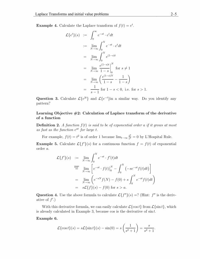
Example 4. Calculate the Laplace transform of f(t) = et.
L{et}(s) :=
∫ ∞
0
e−st · etdt
:= limN→∞
∫ N
0
e−st · etdt
= limN→∞
∫ N
0
e(1−s)t
= limN→∞
e(1−s)t
1 − s
∣∣∣∣N
0
for s �= 1
= limN→∞
(e(1−s)N
1 − s− 1
1 − s
)
=1
s − 1for 1 − s < 0, i.e. for s > 1.
Question 3. Calculate L{e2t} and L{e−t}in a similar way. Do you identify anypattern?
Learning Objective #2: Calculation of Laplace transform of the derivativeof a function
Definition 2. A function f(t) is said to be of exponential order a if it grows at mostas fast as the function eat for large t.
For example, f(t) = t2 is of order 1 because limt→∞ t2
et = 0 by L’Hospital Rule.
Example 5. Calculate L{f ′}(s) for a continuous function f = f(t) of exponentialorder a.
L{f ′}(s) := limN→∞
∫ N
0
e−st · f ′(t)dt
IBP= lim
N→∞
[e−st · f(t)
∣∣N0−∫ N
0
(−se−stf(t)dt)]
= limN→∞
(e−sNf(N) − f(0) + s
∫ N
0
e−stf(t)dt
)= sL{f}(s) − f(0) for s > a.
Question 4. Use the above formula to calculate L{f ′′}(s) =? (Hint: f ′′ is the deriv-ative of f ′.)
With this derivative formula, we can easily calculate L{cos t} from L{sin t}, whichis already calculated in Example 3, because cos is the derivative of sin t.
Example 6.
L{cos t}(s) = sL{sin t}(s) − sin(0) = s
(1
s2 + 1
)=
s
s2 + 1.
Laplace Transforms and initial value problems 2–6
f(t) = L−1{F (s)}(t) F (s) := L{f(t)}(s)
11
s, s > 0
tn, n = 1, 2, ...n!
sn+1, s > 0
sin btb
s2 + b2, s > 0
cos bts
s2 + b2, s > 0
eat 1
s − a, s > a
tneat, n = 1, 2, ...n!
(s − a)n+1, s > a
eat sin btb
(s − a)2 + b2, s > a
eat cos bts − a
(s − a)2 + b2, s > 0
f ′(t) sF (s) − f(0)
f ′′(t) s2F (s) − sf(0) − f ′(0)
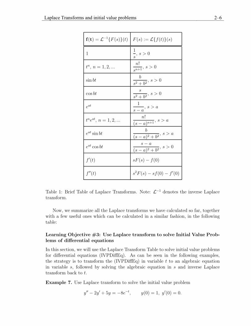
Table 1: Brief Table of Laplace Transforms. Note: L−1 denotes the inverse Laplacetransform.
Now, we summarize all the Laplace transforms we have calculated so far, togetherwith a few useful ones which can be calculated in a similar fashion, in the followingtable:
Learning Objective #3: Use Laplace transform to solve Initial Value Prob-lems of differential equations
In this section, we will use the Laplace Transform Table to solve initial value problemsfor differential equations (IVPDiffEq). As can be seen in the following examples,the strategy is to transform the (IVPDiffEq) in variable t to an algebraic equationin variable s, followed by solving the algebraic equation in s and inverse Laplacetransform back to t.
Example 7. Use Laplace transform to solve the initial value problem
y′′ − 2y′ + 5y = −8e−t, y(0) = 1, y′(0) = 0.

Laplace Transforms and initial value problems 2–7
Let Y (s) := L{y}. Use the Table to obtain
L{y′′} = s2Y (s) − sy(0) − y′(0) = s2Y (s) − s.
L{y′} = sY (s) − y(0) = sY (s) − 1,
L{−8e−t} =−8
s + 1.
Applying Laplace transform to both sides of the DiffEq leads to the following algebraicequation for Y (s):
s2Y − s − 2(sY − 1) + 5Y =−8
s + 1,
⇒ Y (s) =s2 − s − 10
(s + 1)(s2 − 2s + 5).
Use partial fractions
s2 − s − 10
(s + 1)(s2 − 2s + 5)=
A
s + 1+
Bs + C
s2 − 2s + 5
to get
Y (s) =−1
s + 1+
2s − 5
s2 − 2s + 5.
Since y(t) = L−1{Y (s)}, we need to use the Table to inverse transform each the righthand side of the above equation.
L−1
{ −1
s + 1
}= −L−1
{1
s + 1
}= −e−t,
L−1
{2s − 5
s2 − 2s + 5
}= L−1
{2(s − 1) − 3
(s − 1)2 + 22
}
= 2L−1
{(s − 1)
(s − 1)2 + 22
}− 3
2· L−1
{2
(s − 1)2 + 22
}= ???
Question 5. Use the Table to find the solution to the above example. How do youcheck if your answer is correct?
The last example is from an application problem from control theory. We considera servomechanism that models an auto pilot. Such a system applies a torque to thesteering shaft so that an airplane will follow a prescribed direction (angle) g(t). Ascan be expected, the true direction of the airplane y(t) is not always to be the same asthe desired g(t) at all time t. When this happens, the servomechanism will measurethe deviation between y(t) and g(t) and feed back to the steering shaft a torque whichis proportional to the deviation e(t) := y(t) − g(t) but with opposite sign. In thisway, the airplane can stay in the desired course. On the other hand, according toNewton’s second law of motion, the total torque of a rotating object is related to the

Laplace Transforms and initial value problems 2–8
moment of Inertia (denoted by I) of the object and the angular acceleration y′′(t).Hence the servomechanism following the following rule in correcting the direction ofan airplane
Iy′′(t) = −ke(t),
Here k is the positive proportional constant of the correction system.
Example 8. Determine the error e(t) for the auto pilot if the steering shaft is initiallyat rest (y′(0) = 0) in the zero direction (y(0) = 0) and the desired direction is givenby g(t) = a (i.e. a fixed direction=a straight line).
The initial value problem is
Iy′′(t) = −ke(t), y(0) = 0, y′(0) = 0. (1)
Let Y (s) = L{y(t)} and E(s) = L{e(t)}. Since e(t) = y(t) − g(t) = y(t) − a, wehave
E(s) = Y (s) − L{a} = Y (s) − a
s.
Laplace transform both sides of the differential equation (1) to get
L{Iy′′(t)} = I[s2Y (s) − sy(0) − y′(0)] = Is2Y (s) = −kE(s).
Replace Y (s) with E(s) +a
s, we obtain
Is2(E(s) +
a
s
)= −kE(s).
Therefore, E(s) =−Isa
Is2 + k. Inverse Laplace transform E to conclude that
e(t) = −aL−1
{s
s2 + kI
}= −a cos
(√k
It
).
Problems
1. Use Laplace transform to solve the initial value problem
y′′ − 2y′ + 5y = −8e−t, y(0) = 1, y′(0) = 3.
2. Consider the autopilot steering problem given in the last section. Calculatethe error e(t) in the system if the steering shaft is initially at rest in the π/2direction (i.e. y(0) = π/2, y′(0) = 0) and the desired direction is g(t) = a,where a is a constant.
Chapter 3
3 Mathematical Modeling of the Population Growth of a Single Species I – Continuous by Dr. David Rollins Weeks: 2/5 and 2/12 of Spring 2007
Population Growth of a Single Species I – Continous Models 3–2
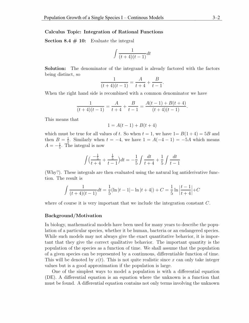
Calculus Topic: Integration of Rational Functions
Section 8.4 # 10: Evaluate the integral
∫1
(t + 4)(t − 1)dt
Solution: The denominator of the integrand is already factored with the factorsbeing distinct, so
1
(t + 4)(t − 1)=
A
t + 4+
B
t − 1.
When the right hand side is recombined with a common denominator we have
1
(t + 4)(t − 1)=
A
t + 4+
B
t − 1=
A(t − 1) + B(t + 4)
(t + 4)(t − 1).
This means that1 = A(t − 1) + B(t + 4)
which must be true for all values of t. So when t = 1, we have 1= B(1 +4) = 5B andthen B = 1
5. Similarly when t = −4, we have 1 = A(−4 − 1) = −5A which means
A = −15. The integral is now
∫ ( −15
t + 4+
15
t − 1
)dt = −1
5
∫dt
t + 4+
1
5
∫dt
t − 1
(Why?). These integrals are then evaluated using the natural log antiderivative func-tion. The result is∫
1
(t + 4)(t − 1)dt =
1
5(ln |t − 1|− ln |t + 4|) + C =
1
5ln∣∣∣∣t − 1
t + 4
∣∣∣∣+C
where of course it is very important that we include the integration constant C.
Background/Motivation
In biology, mathematical models have been used for many years to describe the popu-lation of a particular species, whether it be human, bacteria or an endangered species.While such models may not always give the exact quantitative behavior, it is impor-tant that they give the correct qualitative behavior. The important quantity is thepopulation of the species as a function of time. We shall assume that the populationof a given species can be represented by a continuous, differentiable function of time.This will be denoted by x(t). This is not quite realistic since x can only take integervalues but is a good approximation if the population is large.
One of the simplest ways to model a population is with a differential equation(DE). A differential equation is an equation where the unknown is a function thatmust be found. A differential equation contains not only terms involving the unknown

Population Growth of a Single Species I – Continous Models 3–3
function but also it’s derivatives. An example of a DE with unknown x(t) that alsocontains the first derivative is
x′(t) = 4x(t) + t2
The subject of differential equations is a rich one but we will focus on examples thatcan be solved by integration.
Learning Objective #1: See how a population can be modeled by an ini-tial value problem and see how to solve it by using the partial fractionintegration method.
Simple Growth Model. The simplest model will only concern itself with theeffects of births and deaths. Let x(t) be the species population at any time t. Therate of change of x(t) with respect to time is given by
dx
dt= birth − deaths
Assume that the birth term is proportional to x which is quite reasonable as weexpect the number of births to increase with x. Similarly assume the death term isalso proportional to x. Then our differential equation for x(t) is
dx
dt= bx − μx = (b − μ)x
where b is the per capita birth rate and μ is the per capita death rate. Both theseconstants have the units of time−1. It is natural to define a net growth rate constant
r = b − μ
and then the differential equation for x(t) to be solved is
dx
dt= rx.
Before we solve this let us notice some qualitative features of this equation. Re-member that the population satisfies x(t) ≥ 0 with x(t) = 0 only when the speciesbecomes extinct. Suppose the per capita birth rate is larger than the death rate sothat r > 0. Then we have
dx
dt≥ 0,
which means that x is an increasing function of t. This makes sense since there aremore births than deaths and so the population will grow.
Question 1. Suppose r < 0. What does this mean about births and deaths? Inthis case is x an increasing or decreasing function of time? Explain your answer.
Population Growth of a Single Species I – Continous Models 3–4
Solution:
1. Divide both sides by x:1
x
dx
dt= r
2. Integrate both sides with respect to time t. Note that often, differential equa-tions are solved by integrating.
∫1
x
dx
dtdt =
∫rdt
The left hand integral can be simplified by changing the variable of integrationto x by using the fact that dx = dx
dtdt:
∫ 1
xdx =
∫rdt
The right hand integration is very simple (remember that r is a constant!).The left hand integration is a very simple example of partial fractions with theintegrand already a partial fraction. We get
ln |x(t)| = rt + C
where C is the integration constant. Note that the absolute value symbols arenot required since x(t) > 0. We would like to solve for x(t), so we take theexponential of both sides and get
x(t) = ert+C = eCert = C0ert.
Note that eC is a constant which we will define as C0, that we don’t knowyet. To find C0 we will have give one more piece of information which is calledthe initial condition. Suppose the population is given at some particular time(perhaps by counting) then C0 can be found. Suppose x(0) = 1000 is thestarting population. Then we have
x(0) = 1000 = C0e0 = C0
and the solution is x(t) = 1000ert. A differential equation plus initial conditionis called an initial value problem.
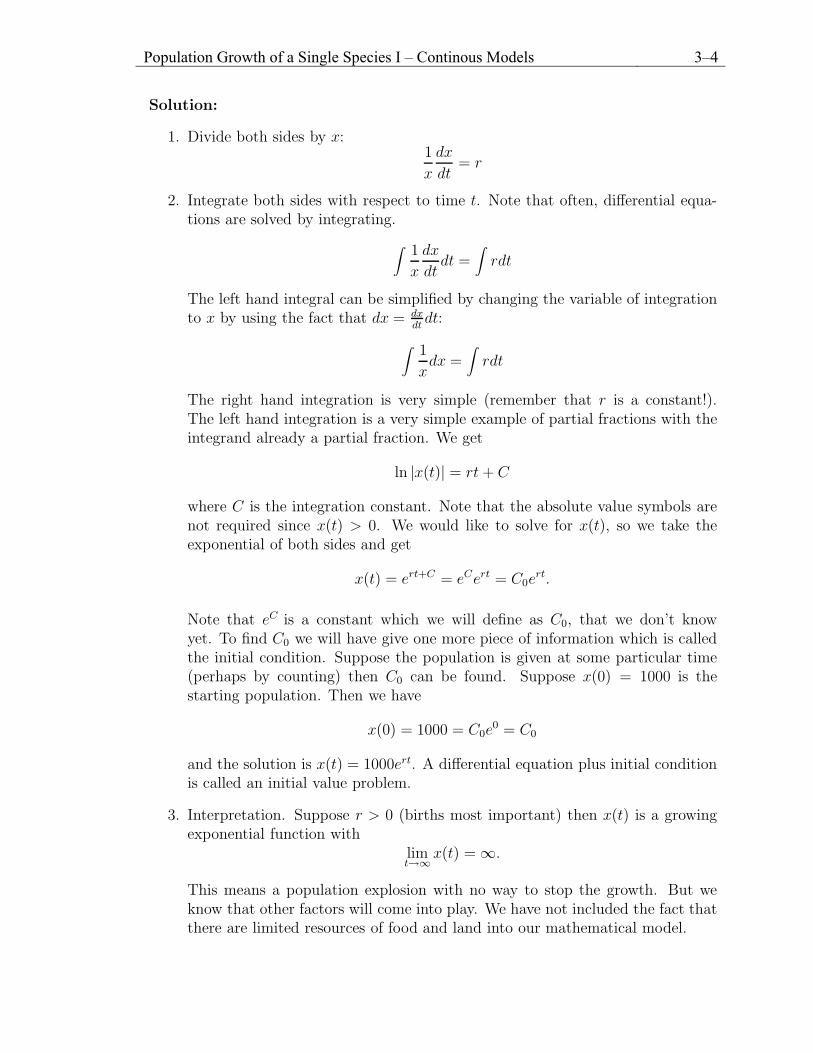
3. Interpretation. Suppose r > 0 (births most important) then x(t) is a growingexponential function with
limt→∞x(t) = ∞.
This means a population explosion with no way to stop the growth. But weknow that other factors will come into play. We have not included the fact thatthere are limited resources of food and land into our mathematical model.
Population Growth of a Single Species I – Continous Models 3–5
Population Growth of a Single Species I – Continous Models 3–6
Note that the equilibrium solutions are x = 0 and x = 1. Following the aboveprocedure
1. Divide both sides by x(1 − x):
1
x(1 − x)
dx
dt= r
2. Integrate both sides with respect to time t. Note that often, differential equa-tions are solved by integrating.
∫1
x(1 − x)
dx
dtdt =
∫rdt
As before, the left hand integral can be simplified by changing the variable ofintegration to x: ∫
1
x(1 − x)dx =
∫rdt
The left hand integration is done by using partial fractions:
1
x(1 − x)=
−1
x(x − 1)=
A
x+
B
x − 1
This implies −1 = A(x − 1) + Bx and gives A = 1 and B = −1. So
∫ (1
x− 1
x − 1
)dt = ln |x|− ln |x − 1| = rt + C.
Combining the logarithms
ln∣∣∣∣ x
x − 1
∣∣∣∣ = rt + C
and inverting we havex
x − 1= eCert = C0e
rt.
Let’s suppose the initial population is x(0) = 2, then the constant C0 can befound
2
2 − 1= C0e
0 ⇒ C0 = 2.
and then x/(x − 1) = 2ert. Since we don’t have x(t) given explicitly we alge-braically solve to get
x(t) =2ert
2ert − 1=
2
2 − e−rt
which is the population of our species for any time t.

Population Growth of a Single Species I – Continous Models 3–7
Population Growth of a Single Species I – Continous Models 3–8
2. Imagine a species that is hunted or fished with a yearly quota specified. In this
case, the differential equation model is modified as follows
dx
dt= rx(1 − x/K) − H
where H is a constant and is called the harvesting rate. Write down the initialvalue problem in the case when the net growth rate is 1, the carrying capacityis 100, the harvesting rate is 21 and the initial population at time zero is 50.
(a) What are the equilibrium solutions?
(b) Find x(t) by integration.
(c) Use algebraic manipulation to find an explicit formula for x(t) includingthe evaluation of the integration constant.
(d) Find the large time limiting behavior and interpret the result from a biolog-ical perspective. How did the harvesting term affect the results comparedwith question 1?
Chapter 4
4 Interactive Graphics Curves using Parametric Equations by Dr. Niels da Vitoria Lobo Weeks: 2/19 and 2/26 of Spring 2007
Interactive Graphics Curves using Parametric Equations 4–2
Calculus Topic: Calculus with Parametric Curves
Section 11.2 # 3: Find an equation of the tangent to the curve at the point.
x = t4 + 1, y = t3 + t, t = −1
Solution: We getdx
dt= 4t3 and
dy
dt= 3t2 + 1.
Hence, the slope of the tangent any tangent is given by
dy
dx=
dy/dt
dx/dt=
3t2 + 1
4t3;
and at t = −1, the slope simplifies to −1. Now, when t = −1, we get x = 2and y = −2. So, using the point–slope form of an equation for a line, namely,y − y0 = m(x − x0), we get y − (−2) = (−1)(x − 2) or y = −x.
Application: Interactive Graphics Curves
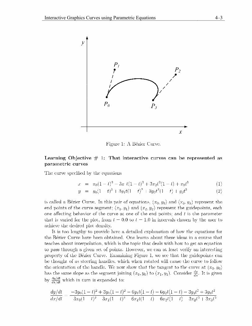
In this section, we discuss how interactive graphics curves can be provided to designersand other users by employing parametric curves (also see the Laboratory Project atthe end of Section 11.2). Interactive graphics curves are often needed that are smooth,and can be conveniently and speedily generated and modified. One such system iscalled Bezier Curves, named after Pierre Bezier (1910 – 1999) a mathematician inthe French automotive industry. A piece of smooth curve is specifiable by giving twopoints P0(x0, y0) and P3(x3, y3), and two guidepoints (like steering handles) P1(x1, y1)and P2(x2, y2). The curve must pass through P0 and P3. The segment joining P0 andP1 defines the direction of the tangent at P0, while the length of this segment definesfor how long the curve starting at P0 should stay close to the tangent. Similarly, forthe segment joining P2 to P3.
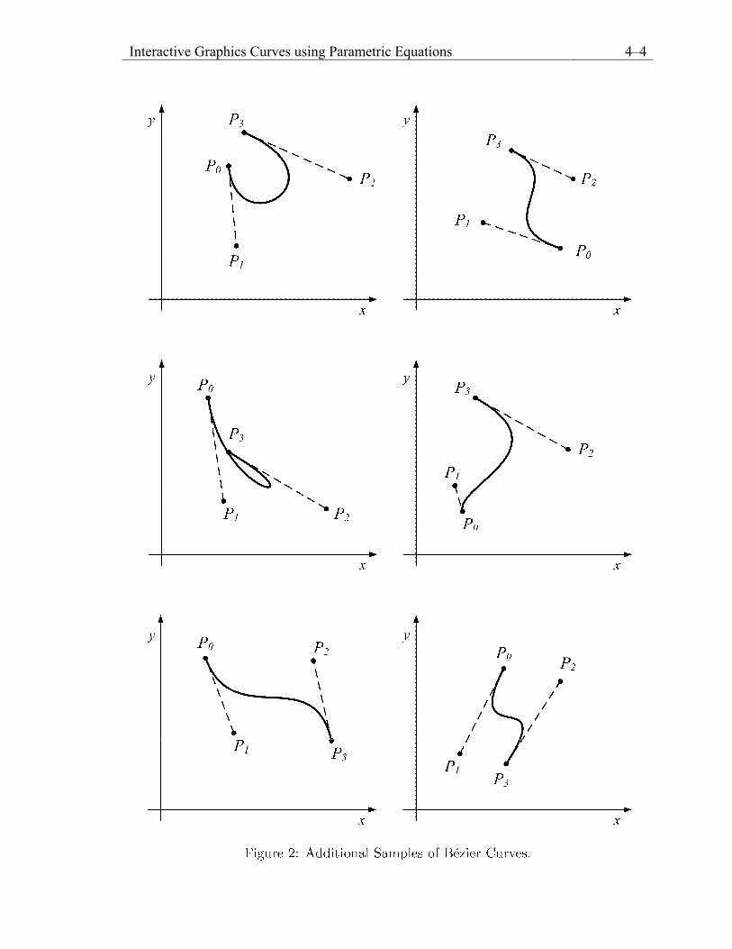
Figure 1 shows an example of such a curve. The user can change the position ofP1 and P2 to change the curve. Figure 2 shows several additional examples of BezierCurves.
Background/Motivation
Interactive graphics curves are used anywhere artists need to design curves that arethen reproducible automatically. One such example is the design of fonts and othersymbols for printers. Other examples include the design of consumer goods such asautomobiles, cell phones, furniture, and the like. In general, complicated curves willbe produced by a chain of several simpler curves, each a Bezier Curve. This allows theuser to change one portion of the complicated curve with little or no effect on otherportions of the overall curve. Once the chain of points is specified for the overallcurve, the user controls the shape of a portion between two consecutive points byplacing two guidepoints for this portion.
The formula to generate the curve is very speedy to execute on a computer, and sothe user can make changes to the design and see the effects of these changes instantly.
Interactive Graphics Curves using Parametric Equations 4–3
Interactive Graphics Curves using Parametric Equations 4–4

Interactive Graphics Curves using Parametric Equations 4–5
Interactive Graphics Curves using Parametric Equations 4–6
Question 2. Draw a symbol similar to the arches in the McDonald’s M. Then,place guidepoints that would have been needed to obtain this symbol.
Learning Objective # 3: To manually follow the plotting procedure fora given specified curve
For the three curves specified next, give the (x, y) coordinates for four intermediatepoints per curve. The first curve is specified by: P0 (3,6); P1 (3.3,6.5); P2 (2.8,3.0);P3 (2,2). The second is specified by: P3 (2,2); P4 (2.5,2.5); P5 (5.8,5.0); P6 (6,6). Thethird is: P6 (6,6); P7 (5.0,5.8); P8 (5.5,2.2); P9 (5,2). Note that your four t choicesper curve will be 0.2, 0.4, 0.6 and 0.8. On graph paper, plot the (16) points, andturn this in along with a list of all the (x, y) coordinates. The manual procedure youare following is one that is automated by Bezier Curve Systems, such as those usedin industry. There are several interactive demos for drawing simple Bezier Curves onthe Internet. Use search terms “Bezier curve demo” to examine some of these. Ifyou leave the word “demo” out, you will also get additional sites where you can readmore about these interesting curves.

Chapter 5
5 Mathematical Modeling of the Population Growth of a Single Species II – Discrete by Dr. David Rollins Weeks: 3/5 and 3/19 of Spring 2007

Population Growth of a Single Species II – Discrete Models 5–2 Calculus Topic: Convergence and Divergence of Sequences
Section 12.1 #19: Determine whether the sequence converges and diverges and ifit converges, determine the limit.
an =2n
3n+1
Solution: The first few terms in the sequence are as follows
a0 =1
3, a1 =
2
32=
2
9, a2 =
22
33=
4
27, a4 =
23
34=
8
81, . . .
By looking at the decimal approximations of these numbers (0.333, 0.222, 0.148,0.098, . . .) we might expect that the sequence will converge to zero in the limit oflarge n. This is made precise by evaluating the limit
limn→∞ an = lim
n→∞2n
3n+1= lim
n→∞1
3
(2
3
)n
= 0
since 2/3 < 1 and the limit of rn as n → ∞ is zero if |r| < 1.
Background/Motivation
Earlier we saw that mathematical models can be used to describe the population ofa particular species, whether it be human, bacteria or an endangered species. Weused a continuous differentiable function to represent the population of a species atany time. We derived a differential equation that when solved by integration gavethe population at any time.
It is also possible to represent the population as a discrete variable xn which givesthe population at the nth time interval. So we can identify the subscript as referringto the time. Generally, we take n = 0, 1, 2, . . ., corresponding to time 0, one timeunit later, two time units later and so on. This can be interpreted as the time unitbetween successive generations of the population, so xn gives the population of thenth generation. The starting population is x0. The population is mathematicallya sequence, with the convergence or divergence property of this sequence determiningthe behavior of the population for large time (n → ∞).
While differential equations are used in the continuous case, difference equationsare used in the discrete case. The solution to a difference equation is a sequence. Dif-ference equations offer the possibility of more complicated population behavior thanthe differential equations we considered. For example, chaotic behavior is possiblewhich was not possible for the simple differential equations we studied in the contin-uous case. Chaotic behavior appears to be random and would mean wild fluctuationsin the species population.
Population Growth of a Single Species II – Discrete Models 5–3
Learning Objective #1: See how a population can be modeled by a dif-ference equation problem and see how to find the sequence and determinethe behavior.
Simple Growth Model. The simplest model will only concern itself with theeffects of births and deaths. Let xn be the population of the nth generation. Assumethat the birth term is proportional to xn which is quite reasonable as we expect morebirths when xn is large. Similarly assume the death term is also proportional to xn.Then our difference equation for xn is
xn+1 = xn + (b − μ)xn = (1 + r)xn
where b is the per capita birth rate, μ is the per capita death rate and r the netgrowth rate constant. This equation says that the population at the next generationis sum of the current population (xn term) plus new growth (or loss) (rxn term) dueto the net growth rate.
Suppose the initial population x0 = 2 and r = 1 so xn+1 = 2xn. Then the sequenceis given by
x1 = 4, x2 = 8, x3 = 16, x4 = 32, . . .
We can clearly see by examining the first few terms of the sequence that xn = 2n+1.We can verify that this in fact solves the difference equation by plugging it in:
xn+1 = 2(n+1)+1 = 2n+2 = 2 · 2n+1 = 2xn
Now we ask whether this sequence converges or diverges.
limn→∞xn = lim
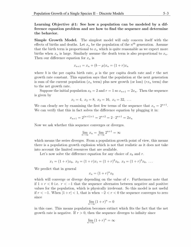
n→∞ 2n+1 = ∞which means the series diverges. From a population growth point of view, this meansthere is a population growth explosion which is not that realistic as it does not takeinto account the limited resources that are available.
Let’s now solve the difference equation for any choice of x0 and r.
x1 = (1 + r)x0, x2 = (1 + r)x1 = (1 + r)2x0, x3 = (1 + r)3x0, . . .
We predict that in generalxn = (1 + r)nx0
which will converge or diverge depending on the value of r. Furthermore note thatif 1 + r < 0 i.e. r < −1 that the sequence alternates between negative and positivevalues for the population, which is physically irrelevant. So this model is not usefulif r < −1. When |1 + r| < 1, that is when −2 < r < 0 the sequence converges to zerosince
limn→∞(1 + r)n = 0
in this case. This means population becomes extinct which fits the fact that the netgrowth rate is negative. If r > 0, then the sequence diverges to infinity since
limn→∞(1 + r)n = ∞
Population Growth of a Single Species II – Discrete Models 5–4
Population Growth of a Single Species II – Discrete Models 5–5

Population Growth of a Single Species II – Discrete Models 5–6
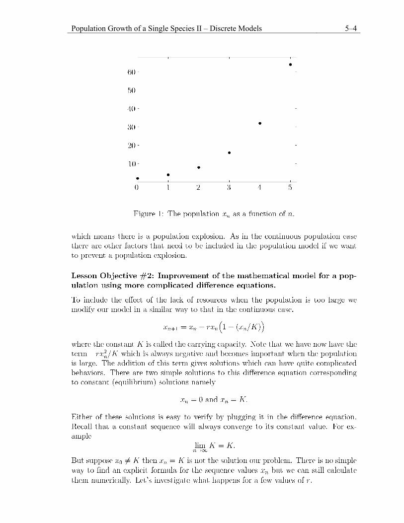
Example 3. Suppose x0 = 2, r = 2.5 and K = 10. Then the difference equation tocalculate the values of xn is:
xn+1 = xn + 2.5xn
(1 − (xn/10)
).
For example x1 = x0+2.5x0(1−(x0/10)) = 2+5(1−(2/10)) = 6. Similar calculationsshow that approximately x2 = 12, x3 = 6, x4 = 12, x5 = 6 and so on. This sequencehas elements that oscillate back and forth between 6 and 12 so the sequence does notconverge. This has the biological interpretation of a population that is periodic intime and repeats itself every two generations. Other periods are also possible for thisdifference equation.
Problems
1. For the model above
(a) Take x0 = 10 and r = 0.5, find the formula for the population xn.
(b) Does the sequence of population values converge or diverge.
(c) What can you conclude from a biological point of view about the long timebehavior of the population?
2. A population is defined by the difference equation
xn+1 =rxn
xn + A
where r and A are constants.
(a) Given x0 = 2, r = 10 and A = 1 find the next four elements in thesequence.
(b) What do you think happens to the population as the number of generationsincreases?
(c) Given x0 = 2, r = 1 and A = 10 find the next four elements in thesequence.
(d) What do you think happens to the population as the number of generationsincreases?
(e) Make an argument similar to that in Example 1 to see what the possibleexact limits should be for this sequence for any value of r and A.

Chapter 6
6 The Geometric Series and Some Applications by Dr. Costas Efthimiou Weeks: 3/26 and 4/2 of Spring 2007
The Geometric Series and Some Applications 6–2
Calculus Topic: The Geometric Series and its Convergence
Background material
Section 12.2 as introduction to series. Pay special attention to Example 5, page 752.The material presented in the following discussion is based on section 12.6 of yourbook.
The ratio and root tests applied to the geometric series. In example 5 ofsection 12.2 it is said that the geometric series
S =∞∑
n=0
xn (1)
converges if |x| < 1. In fact, its limit is
∞∑n=0
xn =1
1 − x.
By setting x = −y, from the discussion in the same example we see that the series
∞∑n=0
(−1)n yn
also converges for |y| < 1 to the sum
S ′ =
∞∑n=0
(−1)n yn =1
1 + y. (2)
Notice that the two results are identical although they may seem different: when x ispositive, y is negative and vice versa. For example, setting x = 1/2 in (1), we find
∞∑n=0
(1
2
)n
= 2 .
Setting y = −1/2 in (2), we find the exact same equation. When x = −1/2, equation(1) gives
∞∑n=0
(−1
2
)n
=2
3.
This result is also recovered from equation (2) for y = 1/2.Now, we would like to re–examine the convergence of the geometric series (1) from
another perspective: that of section 12.6 of your book. The general term of the seriesis an = xn. Then ∣∣∣an+1∣ an
∣∣∣ =
∣∣∣xn+1∣ ∣ xn
∣∣∣ = |x| .
∣
The Geometric Series and Some Applications 6–3
We notice that according to the ratio test, the series S is absolutely convergent when|x| < 1 and divergent for |x| > 1. If x = ±1, the ratio test cannot draw a conclusion.
Similarly, we notice that
n√
|an| = n√
|x|n = |x| .
Therefore the root test also arrives at the same conclusion: the series S is absolutelyconvergent when |x| < 1 and divergent for |x| > 1. If x = ±1, the root test cannotdraw a conclusion either.
Two special series. As noted above, the root and ratio tests cannot say if the twoseries
1 + 1 + 1 + · · · ,
1 − 1 + 1 − · · · ,
converge. However, if we look at the partial sums, we can easily say what the behavioris. For the first series, the partial sums are s1 = 1, s2 = 1+1 = 2, s3 = 1+1+1 = 3, . . .Therefore sn = n and lim
n→∞sn = ∞. For the second series, the partial sums are s1 = 1,
s2 = 1 − 1 = 0, s3 = 1 − 1 + 1 = 1, s4 = 1 − 1 + 1 − 1 = 0. We notice that
sn =
{1 , if n=odd ,0 , if n=even .
However if a sequence {an} converges, then
limn→∞
an+1 = limn→∞
an .
(See exercise 52, page 747 of your book.) If the series was convergent, the aboveequality (applied for the sequence of partial sums) would imply 1 = 0. Therefore theseries is not convergent.
Learning Objectives
In the following section that includes applications of the geometric series, you shouldlearn the following:
1. How series appear in physical problems. The problems we will presentare related to motion of objects. Moreover, for simplicity, we have tried to focuson the geometric series only. However, many different kinds of series appear invirtually all topics in physics.
2. Addition of an infinite number of quantities does not necessarily re-sult in an infinite result: One of the most common misconceptions amongthe students who study physics and have not mastered calculus is that when aninfinite summation is involved, the sum will always be infinite. However, seriesteach us that this is not the case. Adding an infinite number of quantities cangive in some cases a finite number.

The Geometric Series and Some Applications 6–4
3. Memorization of the basic formulæ and theorems: In science there isan enormous amount of information. It is certainly impossible for someoneto memorize all results known to scientists. On the other hand, it is of para-mount importance for someone to recognize the most common situations andknow basic theorems and results. As you work on this project, memorize therelated theorems for series. Also, memorize the basic results and formulæ of thegeometric series; it will be a life–savior for the future.
As you read the next two sections, come back to these learning objectives andensure that you have realized them. In class,
1. I will present several different situations, and I will ask you to explain in whichof them a series will appear.
2. I will give you several series and ask you to apply the root and ratio test to testconvergence.
3. I will give you some geometric series and ask you to find the sum.
Zenon’s Paradoxes
Zenon of Elea (fl. c. 460 BC) was an ancient Greek philosopher who investigatedsome problems dealing with time and space. Their theoretical investigation based oncommon sense seemed to contradict every day reality. Zenon’s paradoxes remainedunresolved in his time. Unfortunately for him, he was lacking many notions thatcalculus introduced much later. In particular, he was lacking the notion of limitsand the methods to sum an infinite number of quantities. Such notions were firstintroduced by Archimedes (Archimedes’ method of exhaustion) and became popularand formal by Newton and Leibnitz1.
I will introduce to you, two of Zenon’s paradoxes. However, I will provide nosolutions! I will let you think about them on your own (and return a written resolutionof one of the two during the second meeting). Their resolution will lead you to a deeperunderstanding of limits and series. In section I will describe another problem and itssolution. You may use this problem as the guiding light for Zenon’s paradoxes.
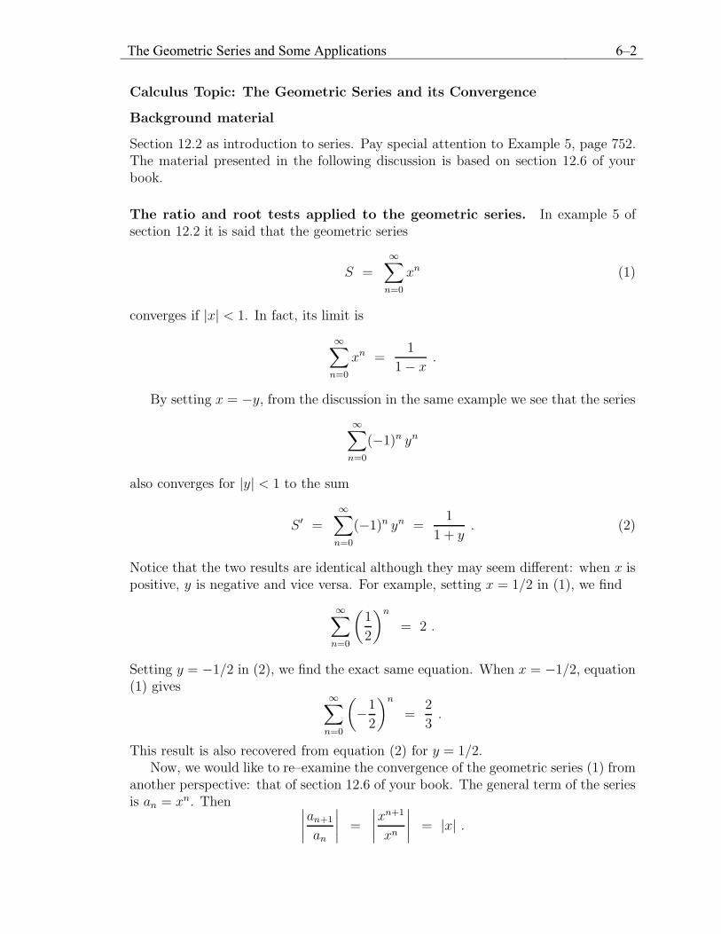
Speedy Achilleas and Turtle. It is said that the great hero of the Trojan warAchilleas could run with the amazing speed of 60 kilometers per hour2. One day hearranged a 120–kilometer race against a fast turtle which could run at the speed of30 kilometers per hour. To make the race fair, the turtle was given a head start of 30kilometers.
The turtle was sure that she was going to win the race. Her reasoning was asfollows. Achilleas starts behind me. By the time Achilleas reaches point T0, I will
1We actually now know that Archimedes had developed and advanced calculus to a great level –1900 years ahead of Newton and Leibnitz but his book was lost. A copy of this work was recentlydiscovered.
2Is this a really fast speed? Estimate the speed of a 100–meter sprinter to compare with.

The Geometric Series and Some Applications 6–5
The Geometric Series and Some Applications 6–6
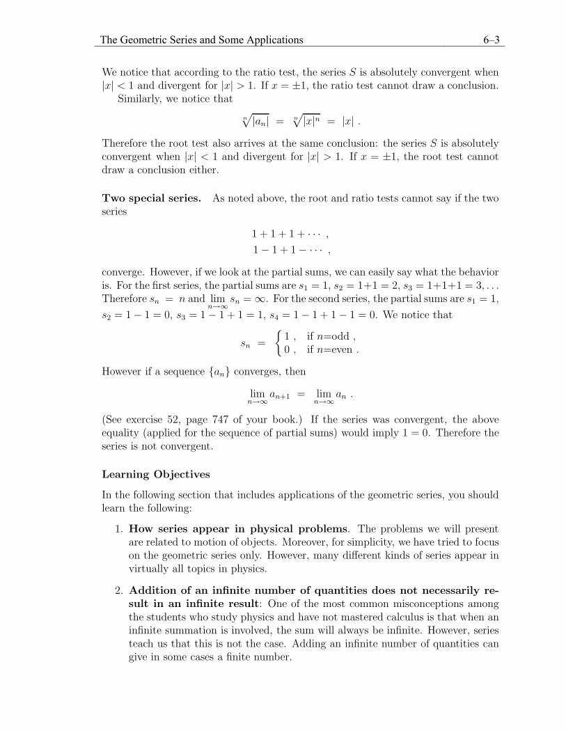
The Geometric Series and Some Applications 6–7

The Geometric Series and Some Applications 6–8
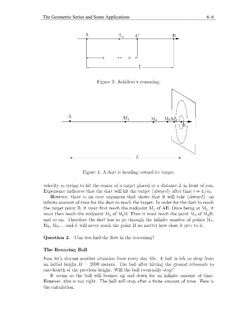
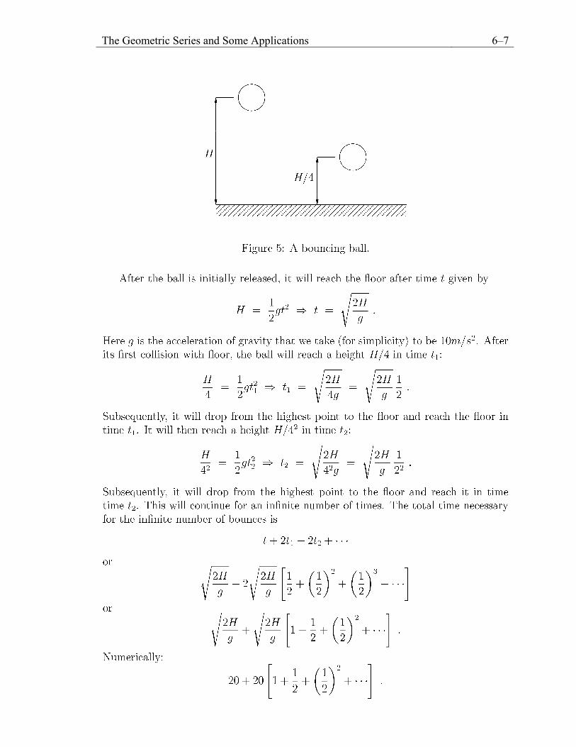
The sum inside the parenthesis is a geometric series that converges to a finite number.Therefore the total time is
20 + 20 × 1
1 − 1/2= 60 seconds .
Question 3. If the ball after each collision with the floor maintains a fractionf (f < 1) of the energy it had before the collision, how much time does it take untilit stops?
Comment
Finally, a comment that may be of some use when you solve the problems: Noticethat in the Achilleas–Turtle race, the speed of Achilleas is twice as much as thatof the Turtle. Similarly, in the dart–target problem, we have selected midpoints.Although these relations are not significant for the conceptual aspect of the problem,they simplify your calculations.
Chapter 7
7 Multipath Effects in Wireless Networks by Dr. Damla Turgut and Chris Sentelle Weeks: 4/9 and 4/16 of Spring 2007
Multipath Effects in Wireless Networks 7–2
Calculus Topic: Taylor and Maclaurin Series
Section 12 #57: Find the sum of the following series. 2 1
2 10
( 1)(2 1)!4
n n
nn n
π +∞
+=
−+∑ .
Solution: Let
xxf sin)( = 0)0( =f xxf cos)(' = '(0) 1f =
xxf sin)('' −= 0)0('' =f xxf cos)(''' −= 1)0(''' −=f
xxf sin)()4( = 0)0()4( =f The Taylor expansion of a function f about the point a is
( ) ( ) ( )
' '' 2 ( )
0
( )( ) ( )( ) ( )( )( ) ( )1! 2! !
!
k k
nn
n
f a x a f a x a f a x af x f ak
f a x an
∞
=
− −= + + + +
−=∑
L−
For ( ) ( )sinf x = x , the expansion about 0a = is
( ) ( )( )
2 13 5 7
0
1sin
1! 3! 5! 7! 2 1 !
n n
n
xx x x xxn
+∞
=
−= − + − + =
+∑L
Now take 4
x π= , so that 1sin
4 2π⎛ ⎞ =⎜ ⎟⎝ ⎠
. Now we have the formula
( )( )
2 1
2 10
112 4 2 1
n n
nn n
π +∞
+=
−=
!+∑
Background/Motivation In this assignment, we are going to discuss Taylor series as they apply to multipath in 802.11 wireless networks. Multipath propagation occurs when radio frequency (RF) signals go through different paths from a source to a destination. A part of the signal travels directly to the destination while another part can bounce off an obstruction such as metal, coated glass, or stone, just as light reflects from a shiny surface before reaching the destination. As a result, part of the signal arrives at the destination via a longer path, incurring delay. This phenomenon is called multipath distortion. The effects of multipath

Multipath Effects in Wireless Networks 7–3
distortion can range from harmless to the cancellation of the signal, depending upon the paths taken by the signal. If the signal received via the longer path has sufficient delay it can interfere with the signal from the direct path resulting in cancellation. On the other hand, the multipath effect can also boost the received signal when both paths arrive in phase such as when multiple transmitting antennas are used.
Multipath interference can be very complex, for example, in an urban environment there are plenty of opportunities for reflections from building structures and automobiles. In the home, the walls, appliances, and furniture introduce numerous opportunities for reflections. In Figure 1, the effect of multipath in an office with a steel desk can be readily observed. This figure is created by simulating the effect of reflections from the RF generated by a transmitter within an office. This is a simple simulation in that only the four walls and steel desk represent opportunities for reflection, while in an actual office the situation would be far more complex. The variations in color represent the fluctuations in signal strength resulting from multipath cancellation as reflections interfere with the energy received directly from the transmitter. All of the dark red areas represent areas where, if an 802.11 receiver were located, the signal strength would be poor while light blue areas represent areas where signal strength would be high. The dark red rectangles represent the steel desk within the room, which represents an area of low intensity because RF energy does not penetrate metal objects. As this shows, a wireless receiver can experience large variations in received signal strength even as it is moved about a small office.
Figure 1: A depiction of multipath in a standard office with a desk looking down on the office. The change in color represents variation in field intensities that occur even in a static environment due to multipath effects within the room. Red indicates weak intensities where cancellation has occurred and blue represent strong intensities.
Multipath Effects in Wireless Networks 7–4
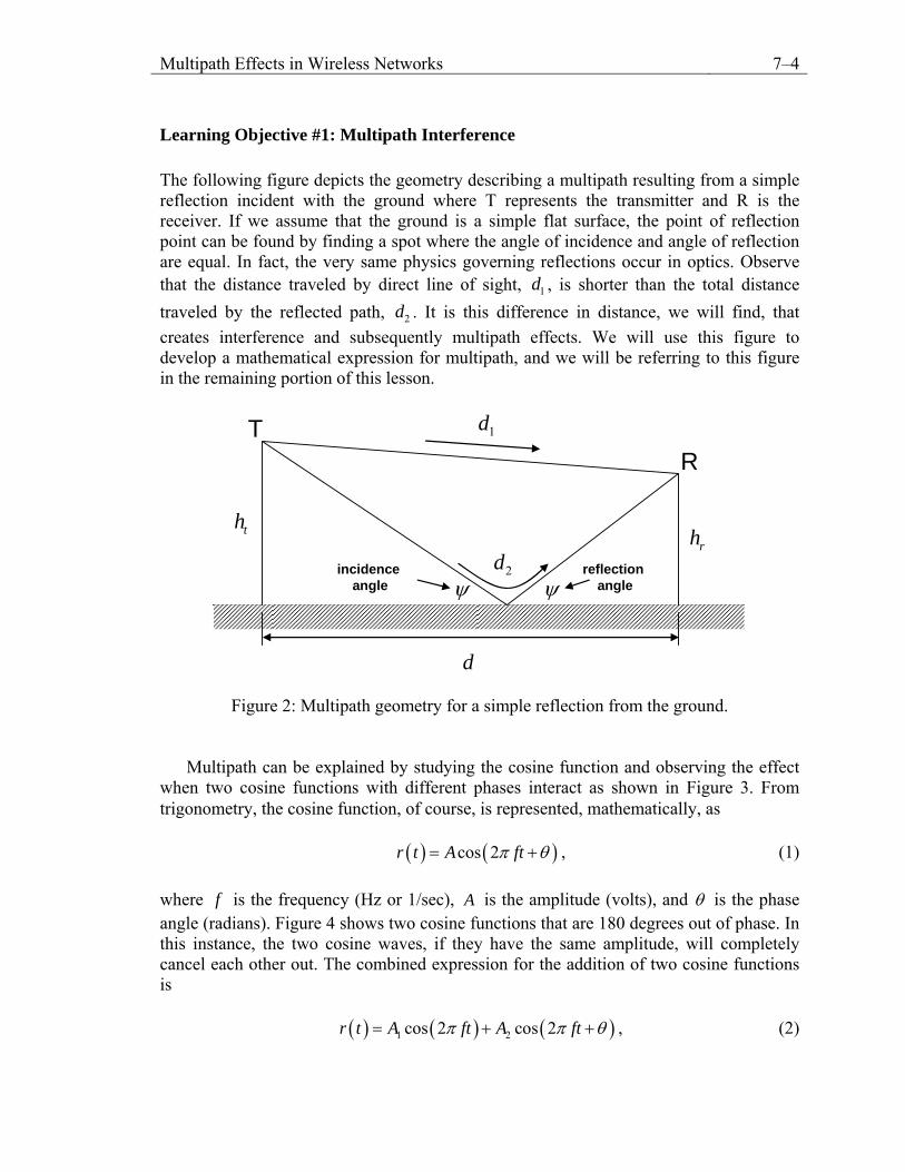
Learning Objective #1: Multipath Interference The following figure depicts the geometry describing a multipath resulting from a simple reflection incident with the ground where T represents the transmitter and R is the receiver. If we assume that the ground is a simple flat surface, the point of reflection point can be found by finding a spot where the angle of incidence and angle of reflection are equal. In fact, the very same physics governing reflections occur in optics. Observe that the distance traveled by direct line of sight, , is shorter than the total distance traveled by the reflected path, . It is this difference in distance, we will find, that creates interference and subsequently multipath effects. We will use this figure to develop a mathematical expression for multipath, and we will be referring to this figure in the remaining portion of this lesson.
1d
2d
1d
2dth
rh
d
ψψ
TR
reflection angle
incidence angle
Figure 2: Multipath geometry for a simple reflection from the ground.
Multipath can be explained by studying the cosine function and observing the effect when two cosine functions with different phases interact as shown in Figure 3. From trigonometry, the cosine function, of course, is represented, mathematically, as ( ) ( )cos 2r t A ftπ θ= + , (1) where is the frequency (Hz or 1/sec), f A is the amplitude (volts), and θ is the phase angle (radians). Figure 4 shows two cosine functions that are 180 degrees out of phase. In this instance, the two cosine waves, if they have the same amplitude, will completely cancel each other out. The combined expression for the addition of two cosine functions is ( ) ( ) ( )1 2cos 2 cos 2r t A ft A ftπ π θ= + + , (2)

Multipath Effects in Wireless Networks 7–5
where θ (radians) represents the difference in phase between the two cosine waves and there is a different amplitude associated with each wave. For two cosine waves that are 180 degrees or π radians out of phase, we get,
( ) ( ) ( )
( ) ( )( ) ( )
1 2
1 2
1 2
cos 2 cos 2
cos 2 cos 2
cos 2
r t A ft A ft
A ft A ft
A A ft
π π π
π π
π
= + +
= −
= −
(3)
and, of course, if the amplitude are equal, then this results in a solution of zero.
0 0.5 1 1.5 2 2.5 3 3.5 4-1
-0.8
-0.6
-0.4
-0.2
0
0.2
0.4
0.6
0.8
1
Am
plitu
de (V
olts
)
Time (seconds) Figure 3: Depiction of two cosine functions with one having a phase shift less than 180 degrees relative to the other.
0 0.5 1 1.5 2 2.5 3 3.5 4-1
-0.8
-0.6
-0.4
-0.2
0
0.2
0.4
0.6
0.8
1
Am
plitu
de (V
olts
)
Time (seconds)
Figure 4: Depiction of two cosine functions that are 180 degrees out of phase.

Multipath Effects in Wireless Networks 7–6
In the case of wireless networking, we are often concerned with knowing the average power of a received signal. The average power (Watts) can be found with the following equation
( )2
2
2
1limT
avg TT
PT→∞
−
= ∫ r t dt (4)
The term represents the instantaneous power of the signal. The value T is the
period (seconds) of the waveform, ( )2r t
( )r t . By integrating the instantaneous power over the period and dividing by the period, we obtain the average power. After calculating the integral, the limit is taken as T approaches infinity, which represents the average power over all time. This limit allows us to compute the average power for a signal that is, perhaps, infinite in duration. The following expression for
T
( )r t describes the addition of two cosine functions having different amplitudes and different phase. ( ) ( ) ( )1 2cos 2 cos 2r t A ft A ftπ π θ= + + (5) Solving for, , we obtain the following avgP
( ) ( ) ( )
( ) ( ) ( ) ( ) ( )
( ) ( )
2 21 2 1 2
2
22 2 2 2
1 2 1 2 1 2
22 2
1 21 2 1 2
1, , lim cos 2 cos 2
1, , lim cos 2 cos 2 2 cos 2 cos 2
, , cos2 2
T
avg TT
T
avg TT
avg
P A A A ft A ft dtT
P A A A ft A ft A A ft ft dtT
A AP A A A A
θ π π θ
θ π π θ π
θ θ
→∞−
→∞−
⎡ ⎤= + +⎣ ⎦
= + + +
= + +
∫
∫ π θ+
Of course, all of the steps have not been shown here, but this is a simple integral to
solve involving a few trigonometric identities and a few substitutions. After solving the integral, the period T drops out preventing the need for solving the limit. This makes sense from the perspective of a cosine function where the average power within the interval will be equal to the average power over all time. We leave the solution of the integral as an exercise for the motivated student.
T
Question 1. Graph the average power as a function of θ if 1 2 1A A= = . Question 2. What happens if the two amplitudes are not equal, i.e., 1 1,A = 2 1 2A = ? Graph the average power as a function of θ .
Multipath Effects in Wireless Networks 7–7
Learning Objective #2: Simple Multipath Example In the case of multipath, the radiated energy from the wireless device, the access point in the example, can be represented as a cosine wave with a frequency of 2.4 GHz or
Hz. Looking again at 92.4 10× Figure 1, we can compare the direct path distance to the receiving node versus the distance of the indirect path where energy is reflected from the ground. We see that the energy reflecting from the ground must travel a longer distance. The longer distance implies that the time of arrival is slightly delayed for the reflected path versus the direct path since the RF energy must travel at the speed of light. It turns out that this delay can be written as a phase as follows.
( ) ( )( ) [( ) ( )
cos 2
cos 2 2
cos 2
d
d
r t A f t
r t A ft f
r t A ft
π τ
]π π τ
π θ
⎡ ⎤= +⎣ ⎦= +
= +
(6)
where, 2 dfθ π τ= . Therefore, the phase of the received signal is a function of the time delay and the frequency of the signal. Of course, the time delay can be computed given the distance and the fact that RF energy must travel at the speed of light as,
ddc
τ = , (7)
where is the distance in meters and c is the speed of light, which is equal to
meters/sec. In our case, we are really interested in the time delay difference between the direct and reflected energy as a function of the difference in distance. Therefore, we can write a new expression of phase as follows with replaced by
.
d83 10×
d
21 dd −
( )1 22d d
fc
θ π−
= , (8)
which shows that if we know the difference in distance covered between the directed and reflected energy, we can compute the phase difference between the two signals. Therefore, the interference resulting from multipath reflection off of the ground can be written as,
( ) ( ) ( )1 21 2cos 2 cos 2 2
d dr t A ft A ft f
cπ π π
⎛ ⎞−= + +⎜
⎝ ⎠⎟ (9)
where the first term on the right hand side of the expression is the energy received directly and the second term is the energy received indirectly.
Multipath Effects in Wireless Networks 7–8
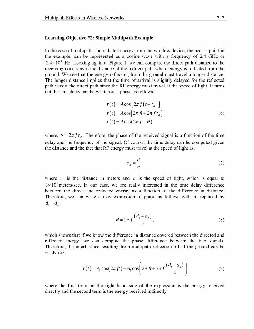
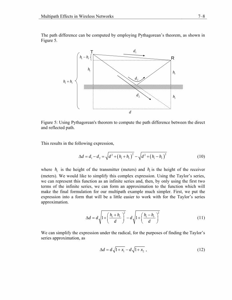
The path difference can be computed by employing Pythagorean’s theorem, as shown in Figure 5.
1d
2d
thrh
TR
2drh
d
t rh h−
t rh h+
Figure 5: Using Pythagorean's theorem to compute the path difference between the direct and reflected path. This results in the following expression,
( ) ( )22 21 2 t r t rd d d d h h d h hΔ = − = + + − + − 2 (10)
where is the height of the transmitter (meters) and is the height of the receiver (meters). We would like to simplify this complex expression. Using the Taylor’s series, we can represent this function as an infinite series and, then, by only using the first two terms of the infinite series, we can form an approximation to the function which will make the final formulation for our multipath example much simpler. First, we put the expression into a form that will be a little easier to work with for the Taylor’s series approximation.
th rh
2 2
1 1t r t rh h h hd d dd d+⎛ ⎞ ⎛Δ = + − +⎜ ⎟ ⎜
⎝ ⎠ ⎝
− ⎞⎟⎠
(11)
We can simplify the expression under the radical, for the purposes of finding the Taylor’s series approximation, as 11 1d d x d x2Δ = + − + , (12)
Multipath Effects in Wireless Networks 7–9
where 2
1t rh hxd+⎛ ⎞= ⎜ ⎟
⎝ ⎠and
2
2t rh hxd−⎛= ⎜
⎝ ⎠⎞⎟ for each part of the expression in (11). The
general Taylor’s series expansion is
( ) ( ) ( ) ( ) ( ) ( )2
1! 2!f a f a
f x f a x a x a′ ′′
= + − + − +L (13)
Since we are trying to approximate (12), we can substitute 0a = in the above equation, that is, we are finding an expansion around the point 0x = .
( ) ( ) ( ) ( ) 20 00
1! 2!f f
f x f x x′ ′′
= + + L+ (14)
Although the Taylor’s series represent the function as an infinite series, the infinite series allows for arbitrary precision and we are only interested in a suitable approximation, therefore, we will take only the first two terms of the Taylor’s series approximation. Equation (14) is also referred to as the Maclaurin series. In general, we can find an approximation to the expression 1 x+ as,
( )
12
00
11 1 12
11 12
xx
x x x
x x
−
→→
+ ≅ + + +
+ ≅ +
x (15)
Therefore, we can now rewrite each radical in (11)
2 21 11 1
2 2t r t rh h h hd d dd d
⎡ ⎤ ⎡+⎛ ⎞ ⎛ ⎞Δ ≅ + − +⎤−
⎢ ⎥ ⎢⎜ ⎟ ⎜ ⎟⎝ ⎠ ⎝ ⎠
⎥⎢ ⎥ ⎢ ⎥⎣ ⎦ ⎣ ⎦
(16)
and, simplifying this expression, we derive the following,
Multipath Effects in Wireless Networks 7–10
( ) ( )
( ) ( )
( )
2 2
2 2
2 2 2 2
1 12 2
12
2 212
1 422
t r t r
t r t r
t r t r t r t r
t r
t r
h h h hd d d
d d
h h h hd
h h h h h h h hd
h hd
h hd
+ −Δ ≅ + − −
⎡ ⎤+ − −= ⎢ ⎥
⎢ ⎥⎣ ⎦⎡ ⎤+ + − + −
= ⎢ ⎥⎢ ⎥⎣ ⎦⎡ ⎤= ⎢ ⎥⎣ ⎦
=
(17)
Therefore, the approximation is
2 r th hdd
Δ ≈ (18)
We can, then, combine this with (8) to obtain
4 t rfh hcd
πθ = (19)
and our expression for the received waveform becomes,
( ) ( )1 24cos 2 cos 2 t rfh hr t A ft A ft
cdππ π⎛= + +⎜
⎝ ⎠⎞⎟ (20)
Of course, we know the general expression for received power level as a function of phase from the previous learning objective, for which we can now substitute in the actual phase for the multipath geometry
( )2 2
1 21 2 1 2
4, , cos2 2
t rfh hA AP A A d A Acd
π⎛= + + ⎜⎝ ⎠
⎞⎟ (21)
It turns out that the amplitude received via the reflected path can be written in terms of the amplitude received via the direct path. In fact, the reflected energy experiences a 180 degrees phase shift as it is reflected from the ground in our problem. Therefore, we can change the expression for received power assuming the reflected amplitude is the negative of the direct amplitude.
( )2 2
2 4, cos2 2
t rfh hA AP A d Acd
π⎛= + − ⎜⎝ ⎠
⎞⎟ (22)
Multipath Effects in Wireless Networks 7–11
( ) 2 2 4, cos t rfh hP A d A Acd
π⎛= − ⎜⎝ ⎠
⎞⎟ (23)
( ) 2 4, 1 cos t rfh hP A d Acd
π⎡ ⎤⎛= − ⎜⎞⎟⎢ ⎥⎝ ⎠⎣ ⎦
(24)
Then, using a trigonometric identity, we can transform equation (24) to
( ) 2 2 2, 2 sin t rfh hP A d Acd
π⎡ ⎤⎛= ⎜⎞⎟⎢ ⎥⎝ ⎠⎣ ⎦
(25)
0 5 10 15 20 250
0.2
0.4
0.6
0.8
1
1.2
1.4
1.6
1.8
2
Distance (meters)
Rec
eive
d si
gnal
stre
ngth
(pow
er)
Rec
eive
d A
vera
ge P
ower
(Wat
ts)
Figure 6: Received signal strength as a function of distance from the transmitter.
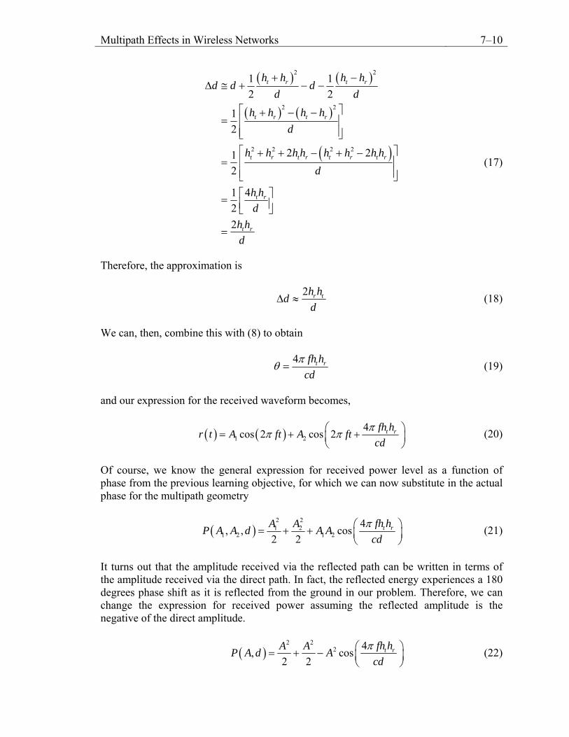
In Figure 6, a plot is made where the amplitude is 1 Volt, 1A = , the frequency is 1 GHz, and the transmitter and receiver are both at 1 meter above the ground. As seen in the figure, the signal strength oscillates at near distances before hitting a peak, at about 13 meters, where a transition from oscillatory behavior to an exponential decay occurs. The point at which the signal first transitions from the oscillatory behavior is referred to as the first Fresnel zone.
We can find the transition point, or first Fresnel zone, by solving for the first derivative of equation (26) and setting this equal to zero as follows,
( ) 2
2
, 8 2 2sin cos 0t r t r t rdP A x fh h A fh h fh hdd cd cd cd
π π π− ⎛ ⎞ ⎛ ⎞= =⎜ ⎟ ⎜ ⎟⎝ ⎠ ⎝ ⎠
(26)
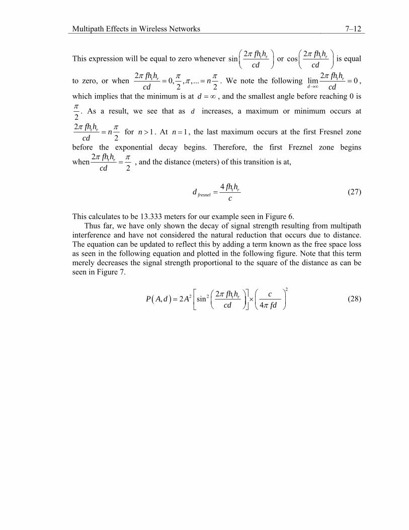
Multipath Effects in Wireless Networks 7–12
This expression will be equal to zero whenever 2sin t rfh hcd
π⎛ ⎞⎜ ⎟⎝ ⎠
or 2cos t rfh hcd
π⎛⎜⎝ ⎠
⎞⎟ is equal
to zero, or when 2 0, , ,...2 2
t rfh h ncd
π π ππ= = . We note the following 2lim 0t r
d
fh hcd
π→∞
= ,
which implies that the minimum is at d = ∞ , and the smallest angle before reaching 0 is
2π . As a result, we see that as increases, a maximum or minimum occurs at d
22
t rfh h ncd
π π= for . At 1n > 1n = , the last maximum occurs at the first Fresnel zone
before the exponential decay begins. Therefore, the first Freznel zone begins
when 22
t rfh hcd
π π= , and the distance (meters) of this transition is at,
4 t rfresnel
fh hdc
= (27)
This calculates to be 13.333 meters for our example seen in Figure 6.
Thus far, we have only shown the decay of signal strength resulting from multipath interference and have not considered the natural reduction that occurs due to distance. The equation can be updated to reflect this by adding a term known as the free space loss as seen in the following equation and plotted in the following figure. Note that this term merely decreases the signal strength proportional to the square of the distance as can be seen in Figure 7.
( )2
2 2 2, 2 sin4
t rfh h cP A d Acd fd
ππ
⎛ ⎞⎡ ⎤⎛ ⎞= ×⎜⎜ ⎟⎢ ⎥⎝ ⎠⎣ ⎦ ⎝ ⎠⎟ (28)
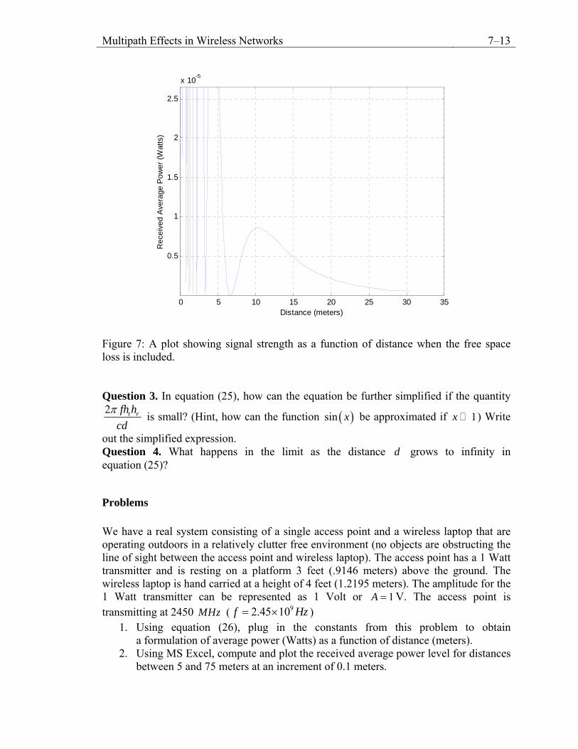
Multipath Effects in Wireless Networks 7–13
0 5 10 15 20 25 30 35
0.5
1
1.5
2
2.5
x 10-5
Distance (meters)
Sig
nal S
treng
thR
ecei
ved
Ave
rage
Pow
er (W
atts
)
Figure 7: A plot showing signal strength as a function of distance when the free space loss is included. Question 3. In equation (25), how can the equation be further simplified if the quantity 2 t rfh h
cdπ is small? (Hint, how can the function ( )sin x be approximated if ) Write
out the simplified expression.
1x
Question 4. What happens in the limit as the distance d grows to infinity in equation (25)?
Problems We have a real system consisting of a single access point and a wireless laptop that are operating outdoors in a relatively clutter free environment (no objects are obstructing the line of sight between the access point and wireless laptop). The access point has a 1 Watt transmitter and is resting on a platform 3 feet (.9146 meters) above the ground. The wireless laptop is hand carried at a height of 4 feet (1.2195 meters). The amplitude for the 1 Watt transmitter can be represented as 1 Volt or 1A = V. The access point is transmitting at 2450 MHz ( 92.45 10f Hz= × )
1. Using equation (26), plug in the constants from this problem to obtain a formulation of average power (Watts) as a function of distance (meters).
2. Using MS Excel, compute and plot the received average power level for distances between 5 and 75 meters at an increment of 0.1 meters.
Multipath Effects in Wireless Networks 7–14
3. Using equation (28), compute the distance where the first Fresnel zone begins (curve transitions from the oscillatory behavior to an exponential decay)?
4. Use the simplification ( )sin x x= for small x to rewrite and simplify equation (29). Note that the simplification is only valid for large distances. How does the average power level vary as a function of d in this equation (describe, no need to plot)? Would this have been as easy to see if the Taylor’s series approximation had not been used to simplify equation (11)? Why?
Appendix: Using Microsoft Excel MS Excel can be used to plot mathematical functions and has the added benefit of being less costly than most of the mathematical software tools such as MATLAB and Mathematica. Due to its availability, it is important to understand the power of MS Excel in solving engineering problems. In this appendix, we will illustrate how to use MS Excel for plotting a function.
In this exercise, we will plot the function ( ) cos 24
x t ft ππ⎛ ⎞= +⎜ ⎟⎝ ⎠
where f is the
frequency in Hz and is the time in seconds. We will set t 910f Hz= for a frequency of 1 . GHz
First, we want to establish the domain of our problem or the x–coordinate. The period of ( )x t is 91 10 seT f −= = c or 1 nsec. If we want to plot ± 4 periods of the function,
then our time should range from 94 10−− × sec to 94 10−× sec. If we want to plot a total of
50 points, our increment should be 9
108 10 1.6 1050
t−
−×Δ = = × . Therefore, we have all of
the information needed to create our plot. Upon launching MS Excel, we are presented with the following.

Multipath Effects in Wireless Networks 7–15
Figure 8: MS Excel with an empty workbook at startup. We are going to be creating two series of data in the first two columns of the Excel spreadsheet. We can start by labeling the series by typing “Time (sec)” in cell “A1” and typing “x(t)” in cell “B1”. Note that the column widths can be changed by selecting the line between two columns such as column “A” and column “B” and right clicking and dragging the line to the desired location.
Figure 9: Entering the column titles for the domain and range.

Multipath Effects in Wireless Networks 7–16
Next, enter the starting value for time by typing “–4E–9” in cell “A2”. Also, the next time will be based upon the increment value. This can be entered as the next time by typing “–3.84E–9” into cell “A3”.
9 104 10 1.6 10 3.84 10− −− × + × = − × 9−
Figure 10: Entering the first two time values in column “A”. Using a shortcut within Excel, the remaining values for time can be automatically filled in. Select both cells “A2” and “A3” by clicking on cell “A2” and holding the left mouse button down while dragging the selection over cell “A3”, and then, releasing the left mouse button so that both cells are highlighted as follows
Figure 11: Result of selecting cells “A2” and “A3”. Note that there is a filled–in box on the bottom right corner of the selection border. When the mouse hovers over this box, the cursor changes to a cross–hair cursor. Click on the box with the left mouse button and while holding the left mouse button, drag the selection across 50 cells so that cells “A2” through “A52” are highlighted with a hash border. The following figure shows highlighting just cells “A2” through “A27”.

Multipath Effects in Wireless Networks 7–17
Figure 12: Result of clicking the lower right corner of the selection in the previous figure and dragging the mouse to cell “A27” while clicking the left mouse button. After all of the cells have been highlighted, release the left mouse button and the incremented values are automatically populated. The value in cell “A52” should be “4.00E–9”.
Figure 13: Results of automatically filling in the time series data.

Multipath Effects in Wireless Networks 7–18
Now we are ready to enter the formula. The formula will be ( ) ( )cos 2 1 94
x t e t ππ⎛ ⎞= +⎜ ⎟⎝ ⎠
,
which can be specified in Excel as, COS(2*PI()*1e9*A2 + PI()/4), if the formula is placed in cell “B2” and “A2” represents time. To enter the formula, type “=COS(2*PI()*1e9*A2 + PI()/4)” in cell “B2”.
Figure 14: Entering the formula into cell “B2”. Once this is done, a shortcut can be used, once again, to populate the remaining values. Do this by first selecting (clicking on) cell “B2” and, then, double click the lower right corner of the cell where the filled in box is located. At this point, all of the values are automatically populated corresponding to entry of time in the “A” column.
Figure 15: Selecting cell “B2” and observing the filled in box at the lower right of the selection border.

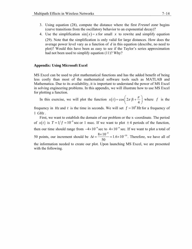
Multipath Effects in Wireless Networks 7–19
Figure 16: Result after double clicking the lower right corner of the selection in the previous figure. To see what happened, click on cell “B3” and observe that the formula was automatically updated to use cell “A3” for time instead of cell “A2”.
Figure 17: Observing the formula in cell “B3”. In order to plot the function, select columns “A” and “B” by clicking on the “A” at the top of column “A” and dragging the selection to column “B” while pressing the left mouse button.

Multipath Effects in Wireless Networks 7–20
Figure 18: Selecting columns “A” and “B”. Once the columns are selected, select the Chart Wizard using the button in the toolbar which depicts a 3D bar graph.
Figure 19: The chart wizard button located in the toolbar. This brings up the wizard. We want to select the XY (Scatter) plot since we are plotting a graph containing both x and y coordinates. From within the XY (Scatter) possibilities, select the chart sub–type which will provide a smooth curve without displaying the points in our data series.
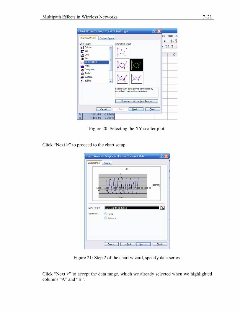
Multipath Effects in Wireless Networks 7–21
Figure 20: Selecting the XY scatter plot. Click “Next >” to proceed to the chart setup.
Figure 21: Step 2 of the chart wizard, specify data series. Click “Next >” to accept the data range, which we already selected when we highlighted columns “A” and “B”.

Multipath Effects in Wireless Networks 7–22
Figure 22: Step 3 of the chart wizard, specify title and axis labels. Fill in the values for the chart title, and x, y axis in step 3 of the wizard and click “Next >” to continue.
Figure 23: Final step of the chart wizard.
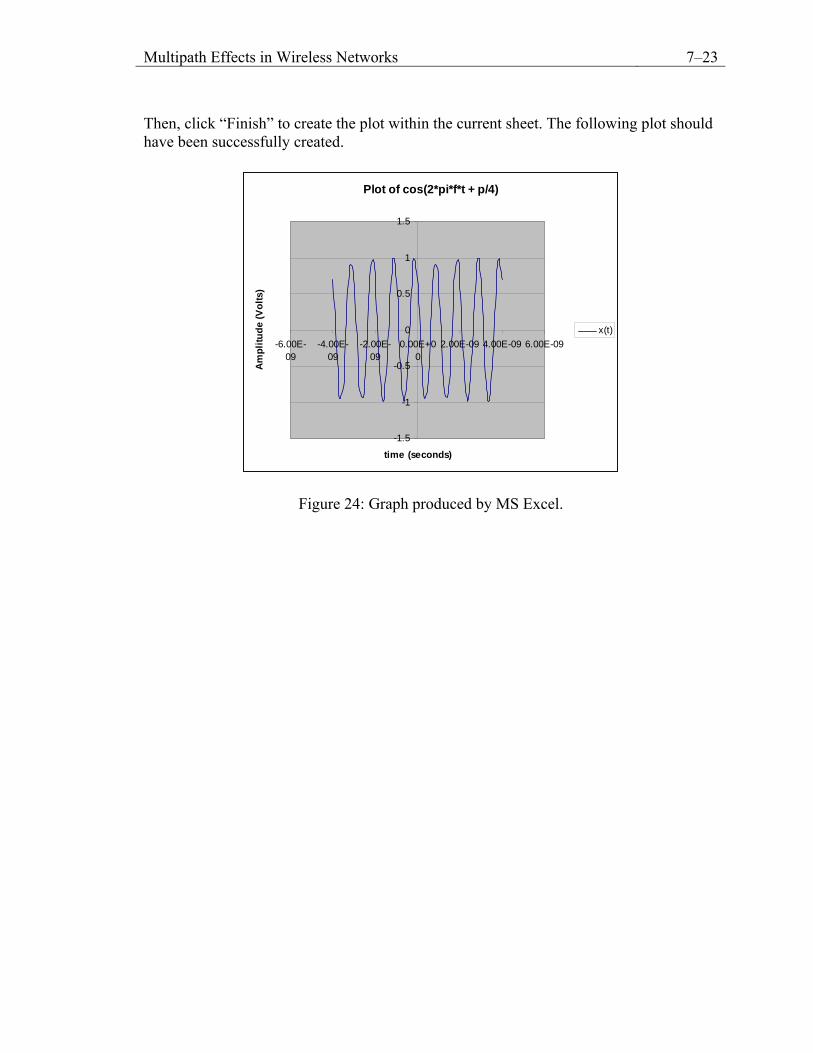
Multipath Effects in Wireless Networks 7–23
Then, click “Finish” to create the plot within the current sheet. The following plot should have been successfully created.
Plot of cos(2*pi*f*t + p/4)
-1.5
-1
-0.5
0
0.5
1
1.5
-6.00E-09
-4.00E-09
-2.00E-09
0.00E+00
2.00E-09 4.00E-09 6.00E-09
time (seconds)
Ampl
itude
(Vol
ts)
x(t)
Figure 24: Graph produced by MS Excel.