applications and limitations of constrained high
TRANSCRIPT
Atmos. Meas. Tech., 9, 3263–3281, 2016www.atmos-meas-tech.net/9/3263/2016/doi:10.5194/amt-9-3263-2016© Author(s) 2016. CC Attribution 3.0 License.
Applications and limitations of constrained high-resolution peakfitting on low resolving power mass spectra from the ToF-ACSMHilkka Timonen1, Mike Cubison2, Minna Aurela1, David Brus1, Heikki Lihavainen1, Risto Hillamo1,Manjula Canagaratna3, Bettina Nekat4, Rolf Weller3, Douglas Worsnop3, and Sanna Saarikoski11Atmospheric composition research, Finnish Meteorological Institute, Helsinki, Finland2TOFWERK AG, Thun, Switzerland3Aerodyne Research Inc., Billerica, MA, USA4The Alfred Wegener Institute, Helmholtz Centre for Polar and Marine Research, Bremerhaven, Germany
Correspondence to: Hilkka Timonen ([email protected])
Received: 15 January 2016 – Published in Atmos. Meas. Tech. Discuss.: 2 March 2016Revised: 31 May 2016 – Accepted: 22 June 2016 – Published: 25 July 2016
Abstract. The applicability, methods and limitations of con-strained peak fitting on mass spectra of low mass resolv-ing power (m/1m50 ∼ 500) recorded with a time-of-flightaerosol chemical speciation monitor (ToF-ACSM) are ex-plored. Calibration measurements as well as ambient dataare used to exemplify the methods that should be appliedto maximise data quality and assess confidence in peak-fitting results. Sensitivity analyses and basic peak fit metricssuch as normalised ion separation are employed to demon-strate which peak-fitting analyses commonly performed inhigh-resolution aerosol mass spectrometry are appropriateto perform on spectra of this resolving power. Informationon aerosol sulfate, nitrate, sodium chloride, methanesulfonicacid as well as semi-volatile metal species retrieved fromthese methods is evaluated. The constants in a commonlyused formula for the estimation of the mass concentrationof hydrocarbon-like organic aerosol may be refined basedon peak-fitting results. Finally, application of a recently pub-lished parameterisation for the estimation of carbon oxida-tion state to ToF-ACSM spectra is validated for a range oforganic standards and its use demonstrated for ambient ur-ban data.
1 Introduction
Atmospheric aerosols influence health, climate and visibil-ity (Pope and Dockery, 2006; IPCC, 2013). All these influ-ences are tightly linked with particulate matter (PM) concen-
tration and PM chemical composition (IPCC, 2013). Tradi-tionally, aerosol composition was studied by collecting par-ticulate matter on a filter substrate for an extended periodranging from hours to days and subsequent composition anal-ysis in laboratory. Development of online analysis instru-ments, particularly based on aerosol mass spectrometry, hasenabled the measurement of chemical composition of PM inreal time. The Aerodyne aerosol mass spectrometer (AMS;Jayne et al., 2000; DeCarlo et al., 2006) is designed to pro-vide detailed information on size-resolved aerosol chemicalcomposition for short- to medium-term campaigns (weeks tomonths); however, it is not suitable for long-term monitoringwithout the presence of an operator. The Aerodyne aerosolchemical speciation monitor (Q-ACSM; Ng et al., 2011b) isbased on AMS technology but adapted for long-term moni-toring; however, the quadrupole detector limits the mass re-solving power to unity and provides reduced sensitivity com-pared with the AMS. A recently developed version of this in-strument employing time-of-flight (ToF) detection providesgreater sensitivity and mass resolving power of around 500(ToF-ACSM; Fröhlich et al., 2013). Whilst the increase insensitivity relative to the Q-ACSM is an obvious advantagefor measurements in clean locations such as Antarctica or forincreasing temporal resolution, the limits of potential extrainformation afforded by the increased mass resolving power,and in particular the associated uncertainties on peak-fittingparameters, are as yet unexplored in literature.
In analysis of high-resolution AMS data, peak fittingis typically employed to retrieve signal intensities of ions
Published by Copernicus Publications on behalf of the European Geosciences Union.

3264 H. Timonen et al.: Constrained peak fitting of ToF-ACSM data
whose peaks overlap in the mass spectrum, expanding greatlythe content and quality of information that may be extractedfrom the data in comparison to simple peak integration(e.g. DeCarlo et al., 2006; Aiken et al., 2008). Fröhlich etal. (2013) demonstrated that peak fitting could be applied toToF-ACSM data and presented a simple example for a singleisobaric peak, but the extent and limitations of the applicabil-ity of the technique were not explored. This paper addressesthe question of what extra information can be obtained by fit-ting the MS peaks. Recently, the uncertainty on fitted peak in-tensity associated with the constrained peak-fitting procedureemployed by the AMS community has been explored andparameterisations for calculation of the precision reported(Corbin et al., 2015; Cubison and Jimenez, 2015). These areused, together with the appropriate sensitivity analyses, to as-sess the confidence in the peak-fitting results and draw con-clusions on the appropriateness of applying peak fitting forretrieval of overlapping ion peak intensities for a range ofexample scenarios measured with a ToF-ACSM.
2 Experimental
2.1 Time-of-flight aerosol chemical speciation monitor
The ToF-ACSM (Fröhlich et al., 2013; Aerodyne ResearchInc., Billerica, USA) is designed for long-term monitor-ing of submicron aerosol composition with temporal reso-lution of typically 10 min (and up to 1 Hz) and mass re-solving power m/1m50 of typically 500 (and up to 600).Based on the sampling technology of the ToF-AMS (time-of-flight aerosol mass spectrometer; Drewnick et al., 2005;DeCarlo et al., 2006), the ToF-ACSM contains a critical ori-fice to constrain the flow (1.4 cm3 s−1) and an aerodynamiclens to focus submicron particles into a narrow beam intro-duced into a differentially pumped vacuum chamber wherethe gas molecules tend to diverge from the beam path and arepumped away, concentrating the aerosol : gas molecule ratioby a factor of around 107. The particle beam impacts a heatedplate held at 600 ◦C and the molecules are vaporised and im-mediately ionised using 70 eV electron impact (EI) ionisa-tion. The ions are introduced into a compact time-of-flightmass analyser (ETOF, TOFWERK AG, Thun, Switzerland)and extracted orthogonally using pulsed extraction for even-tual detection with a discrete dynode detector. Mass spec-tra are recorded with and without the use of a filter in theinlet line; the resulting difference in recorded signal is pre-scribed to the aerosol. These signals are converted to nitrateequivalent mass concentrations using the same ionisation ef-ficiency calibration procedure utilised for the AMS and de-scribed by Jimenez et al. (2003). Post-processing was per-formed using the data analysis package “Tofware” (version2.5.3, www.tofwerk.com/tofware) running in the Igor Pro(Wavemetrics, OR, USA) environment.
2.2 Measurement locations and datasets
Three ToF-ACSM datasets were used to study the applica-bility and limitations of constrained peak fitting on massspectra recorded with the ToF-ACSM, measured in cleanbackground conditions (Neumayer, Antarctica), in the urbanbackground (SMEAR III) and in an industrial environment(underground mine, Kemi).
2.2.1 Helsinki, Finland
ToF-ACSM measurements were conducted at the SMEARIII measurement station in Helsinki, Finland, from 2 to 8March 2014. The SMEAR III station (Station for MeasuringEcosystem–Atmosphere Relationships; 60◦12′ N, 24◦57′ E;30 m a.s.l.; Järvi et al., 2009) is an urban background mea-surement station for the long-term measurement and inves-tigation of chemical and physical properties of atmosphericaerosols and trace gases, meteorological parameters and tur-bulent fluxes. The station is situated on the Kumpula cam-pus, 5 km northeast from the centre of Helsinki. Approx.200 m east of the station is a major road with heavy traf-fic (60 000 cars day−1). A collection efficiency of 0.5 was as-sumed based on previous studies conducted on SMEAR IIIstation, e.g. Aurela et al. (2015). During the measurement pe-riod presented here the PM concentrations exhibited a meanaverage of 16.2 µg m−3. However, larger concentrations upto 45 µg m−3 were observed (Fig. S1).
2.2.2 Antarctica
ToF-ACSM measurements were conducted at the NeumayerIII station in Antarctica (70.6744◦ S, 8.2742◦W; http://www.awi.de/en/go/air_chemistry_observatory; Weller et al., 2011)during the Antarctic summer from December 2014 to Febru-ary 2015. Located far from primary emission sources, theNeumayer III station is an ideal location for conductingbackground measurements free from anthropogenic influ-ences (Weller et al., 2015). The two most frequently observedclasses of aerosol observed in Antarctica contain sulfur andsea salt. Sulfur-containing particles, whose secondary pro-duction in the atmosphere is controlled by pathways includ-ing photochemical reactions involving dimethyl sulfide emit-ted by the oceans, dominate particle number concentrationsin the Antarctic atmosphere most of the time (Korhonen etal., 2008; Weller et al., 2011).
Very low background aerosol concentrations of less than1 µg m−3 were typically measured, consisting almost purelyof sulfate and chloride compounds. Larger PM concentra-tions were observed during January and February (up to3 µg m−3) when the temperature was higher and the adjacentocean ice free. We have chosen two distinct episodes for usein analyses presented in this work. Each exhibited differentcharacteristics and posed different problems for extractinginformation from the data using peak fitting. Episode 1 (2–
Atmos. Meas. Tech., 9, 3263–3281, 2016 www.atmos-meas-tech.net/9/3263/2016/

H. Timonen et al.: Constrained peak fitting of ToF-ACSM data 3265
3 December 2014) represents emissions from sea areas andhad elevated chloride concentrations. During episode 2 (7–13 January 2015) elevated sulfate and methanesulfonic acid(MSA) concentrations were observed.
2.2.3 Underground mine
ToF-ACSM measurements were conducted at the Kemi Mine(Outokumpu Chrome Oy) 500 m below the surface duringthe spring of 2014 as a part of a project aiming to help devel-opment of a sustainable and safe mining environment. Themain sources of particles in the underground mine were theore extraction and processing for coarse particles and dieselexhausts from mining machinery and transport vehicles forsubmicron particles. A subset of the data is used here in or-der to test peak fitting on information-rich mass spectra takenin an environment with high PM concentrations.
3 Methods
3.1 Peak-fitting methodology
The post-processing software “Tofware” utilised for ToF-ACSM analysis uses a peak deconvolution routine where thepeak positions are defined a priori and held fixed in the fittingprocedure, based on the methodology utilised by the PIKAsoftware of the ToF-AMS community (DeCarlo et al., 2006;Sueper, 2008). EI ionisation, as is used in the ToF-ACSM,tends to ionise and fragment the molecules in a very con-sistent manner. Thus, 1 degree of freedom is removed fromthe ion fitting procedure, which can be based upon a com-prehensive list of ions and their exact m/Q that define thefitted centroid values. Furthermore, the peak model (widthand shape) is held fixed for a given isobaric mass and themass calibration is also defined a priori and held constant.The only parameter to vary is thus peak intensity, for whichthe optimal values for all peaks at a given isobar are ascer-tained by non-negative least-squares optimisation using theactive set method of Lawson and Hanson (1995). We presenthere a detailed description of each step in the setup of thepeak-fitting routine, with exception of the mass calibration,which is discussed at length in the following section.
3.1.1 Mass spectral baseline subtraction
Mass spectra recorded using analogue-to-digital convertersto digitise the detector signal for data acquisition purposes,as is the case in the ToF-ACSM, can be expected to ex-hibit a non-zero mass spectral baseline as a result of back-ground ions and, potentially, electronic noise (Fig. 1). In ad-dition, peaks adjacent to large signals (such as N+2 in the ToF-ACSM) can be expected to be superimposed upon a signifi-cant baseline varying in intensity with m/Q. It is importantto subtract this baseline from the mass spectrum before car-rying out the peak fit procedure. As it is desired to let the
Figure 1. Example of a mass spectral baseline determined using themethodology described in the text.
analysis software execute peak fitting as a batch process uponlarge numbers of mass spectra, a parameterisation is requiredwhich can reliably generate the MS baseline based on onlya few tuneable parameters. Tofware achieves this through asimple two-step process:
i. a low-pass filter is applied to the MS to remove noise;
ii. a running box average of the de-noised MS is generatedbased not on the mean but on the lowest data point inthe box.
Provided the box width is set large enough such that it ex-tends over the entire width of a typical MS peak, step (ii)effectively interpolates over the peaks as it takes the lowestdata point at each step. Step (i) has the effect of ensuring thecalculated baseline tends to run through the centre and notalong the bottom edge of the noise. By default, the width ofthe box is set to 40 mass spectral data points (50 ns). It is pos-sible that, in regions adjacent to large peaks with significantgradients, the box method generates a baseline slightly lowerthan the optimum. However, the peak most significantly im-pacted by this effect, NO+, the negative offset is observed tobe at most 5 % of peak height and typically lower. This off-set is also removed during calculation of the difference spec-trum, although it does contribute to a slightly higher impreci-sion. The low-pass filter (Zahradník and Vlcek, 2004) used instep (i) removes by default frequencies higher than 16 GHz.We note that sometimes the baseline might not be reachedbetween large peaks, especially at higher m/Q range. ForToF-ACSM mass range (up to m/Q∼ 200) this is, however,not an issue.
3.1.2 Determination of instrumental transfer function(peak model)
Peak width
The width of an isolated ion peak is expected to observe a lin-ear relationship with m/Q. A scatter plot of peak width vs.m/Q for isolated ions will thus highlight MS peaks that rep-resent multiple, overlapping, ions as they will lie above the
www.atmos-meas-tech.net/9/3263/2016/ Atmos. Meas. Tech., 9, 3263–3281, 2016

3266 H. Timonen et al.: Constrained peak fitting of ToF-ACSM data
0.35
0.30
0.25
0.20
0.15
0.10
0.05
0.00
Full-
wid
th a
t h
alf
-maxi
mu
m
150100500
600
400
200
0
150100500
Fit for p
eak a
t mo
use
ptr
15.115.014.9
Peaks used in fit, sized by intensity
Peak width function
m Q-1 m dm as f (m Q )-1 -1
Figure 2. Ascertaining the peak width as a function of m/Q: thestraight-line fit (peak width function, in red) is applied to the chosendata points (in black), giving the relationship for mass resolvingpower shown bottom-right. The principle behind this methodologyis that isolated ions (in black) should exhibit narrower peak widthsthan those with adjacent ions (in grey).
linear regression line (Meija and Caruso, 2004) as shown inFig. 2. Junninen et al. (2010) and Stark et al. (2015) both usedthis effect to develop peak width parameterisations for use inatmospheric science analysis software; an adapted version ofthe method of Stark et al. (2015) is utilised here. Müller etal. (2013) report on a robust method for peak width calcula-tion in proton mass-transfer mass spectrometry which utilisesthe same list of known isolated ions as the mass calibration.A similar method could certainly be employed for the lowerpart of the ToF-ACSM mass spectrum but would require ex-trapolation to high m/Q. To constrain the upper end of thelinear regression, the following steps are taken:
i. the N most intense peaks in the spectrum are found,where N is the largest m/Q measured divided by 3;
ii. a single Gaussian is fitted to each MS peak;
iii. a straight-line fit is applied to the scatter plot of fullwidth at half maximum vs. m/Q;
iv. step (iii) is iterated, removing the point that lies the fur-thest above the fit line, until 10 peaks remain.
The user may choose additional peaks to use at step (iv),and has the option to manually remove any points from thelinear fit of step (iii). Peak width is not expected to varygreatly over time other than with changes in instrument tun-ing. Thus the default peak width is calculated automaticallyfor each 24 h data file, but the user can define a revised ver-sion, typically once for each set of instrument tuning param-eters during an experimental campaign, and save this in thedata files for future use.
Peak shape
Owing foremost to the energetic primary ion beam, the mea-sured shape of the ion peaks in the ToF-ACSM mass spec-
trum is often distinctly non-Gaussian and not easily de-scribed using mathematical functions. Therefore, rather thanattempt to reduce the observed shape to a combination offunctions, each peak is represented with a custom peak shapefunction following the high-resolution time-of-flight aerosolmass spectrometer (HR-ToF-AMS) methodology proposedby DeCarlo et al. (2006) and adapted for use in multipleatmospheric science analysis packages (Sueper, 2008; Jun-ninen et al., 2010; Müller et al., 2013; Stark et al., 2015).The ToF-ACSM peak shape is determined using the follow-ing routine:
i. the 20 largest peaks in the spectrum are found and asingle Gaussian fitted to each;
ii. the measured shape of the peak is normalised to the fit-ted Gaussian width;
iii. the second derivative of each normalised peak is anal-ysed and peaks with shoulders are discarded (Fig. S2);
iv. all the remaining normalised shapes are averaged togenerate the custom peak shape.
The user may additionally choose to fit more/fewer peaksat step (i) and has the option to apply additional constraintssuch as monotonicity and thresholds on the min/max ioncounts. The custom peak shape is typically defined once foreach set of instrument tuning parameters during an experi-mental campaign and is saved in the data files for future use.
The assumption of consistent peak shape has been widelyemployed in the atmospheric community (e.g. Cappellin etal., 2011); nonetheless this does not prove its validity. Notethat this is not the case for ions that do not originate in thesource plume, such as K+ ions stemming from surface ioni-sation on the ToF-ACSM heater. User error – i.e. an incorrectdefinition of peak shape – is also a potential source of errorand arguably of greater probability and magnitude than anypotential instrumental artefacts. A comprehensive study ofthe impact of a varying or incorrectly determined peak shapewould be a useful addition to the literature. However, to high-light the validity of the invariant peak shape assumption forthis study, we (i) verified that the peak shape was invariantover a large mass range by comparing the shape for knownisolated ions in a calibration measurement where SF6 gas wasinjected at the ioniser (see Fig. S3) and (ii) verified that thepeak shape was invariant over time by comparing the shapeof the N+2 peak for nearly a month of data (Fig. S4).
3.1.3 Peak list
For HR-ToF-AMS data, the list of ion peaks to be utilisedduring peak fitting has been assembled and extended overa decade of instrument development and is quite compre-hensive in nature (Sueper, 2008). Most of these ions are,however, unresolvable with the mass resolving power of the
Atmos. Meas. Tech., 9, 3263–3281, 2016 www.atmos-meas-tech.net/9/3263/2016/

H. Timonen et al.: Constrained peak fitting of ToF-ACSM data 3267
ETOF-equipped ToF-ACSM, which precludes use of the HR-ToF-AMS ion list. The particular ions to fit must thereforebe carefully considered based on targeted analyses, ratherthan taking the blanket approach of fitting everything. In theresults section we present multiple case studies highlight-ing the state-of-the-art knowledge of which ions/ion groupsare appropriate for inclusion in peak-fitting analyses of ToF-ACSM data.
3.2 Mass calibration
ToF-ACSM measurement profiles are typically convertedfrom time-of-flight to mass-to-charge space and vice versausing the numerical relationship ToF= a+ b×
√(m/Q),
where a and b are constants. In the constrained peak-fittingprocedure employed during ToF-ACSM and AMS analysis,the accuracy and precision of the mass calibration are of crit-ical importance, because the fitting is performed in time-of-flight space and the position of the fitted peaks held constantusing fixed mass-to-charge values. In consequence, an imper-fect mass calibration introduces imprecision in the fitted peakintensities, particularly for weaker signals in the presenceof larger neighbours (Cubison and Jimenez, 2015), althoughimprecision in the fitted intensity is a significant source of er-ror even for isolated peaks (Corbin et al., 2015). In practice,the precision of the mass calibration is limited principallyby (i) the spectrometer resolving power, for wider calibrantpeaks have a less well-defined centroid position, (ii) countingstatistics for the calibrant ions, and, non-ideally, (iii) the in-fluence of neighbouring ions on assessment of calibrant peakposition. Since (i) is limited by the hardware, it may be con-sidered an intrinsic limitation during data analysis. Whilstnarrower peaks would improve the fitted peak positions, themeasured peak width is of course fixed during analysis andthus plays no role in the parameters that a user may tuneto optimise the mass calibration. However, (ii) and (iii) areworth consideration as they can significantly degrade cali-bration accuracy. We note that Corbin et al. (2015) demon-strate that the AMS calibration can also contain biases thatare of similar magnitude as the imprecision; considerationof their sources is, however, outside the scope of this paper.Finally, it is emphasised that this discussion pertains to fittedpeaks and these effects would not introduce appreciable errorin integrated isobaric peak intensities (processing of the full-resolution mass spectra to centroid, or “stick”, spectra basedon unit-mass resolution integration boundaries).
3.2.1 Effect of counting statistics
A significant source of calibration imprecision during mon-itoring operation can be counting errors. In the lower massrange of the ToF-ACSM spectrum, several large signals aris-ing from air and water ions (typically H2O+, N+2 , O+2 andCO+2 ) may be used for mass calibration. Constraining theupper end is, however, significantly more challenging and
is typically achieved by including the tungsten ions in thecalibrant peak list. As the ToF-ACSM is usually operatedat half the emission current of the AMS (to maximise fila-ment lifetime), these are weak signals and subject to a sig-nificant level of noise from counting error. Unfortunately,the inclusion of even one weak ion in the mass calibrationpeak list greatly increases calibration imprecision (Cubisonand Jimenez, 2015). A similar simulation of the mass cali-bration routine used in that study was employed here to as-sess the impact of the weak W+ signal on the ToF-ACSMmass calibration imprecision. Comparison of the N+2 and W+
ion signals for several ambient ToF-ACSM datasets indicatesa ratio N+2 /W+ ∼ 50 000. Assuming a typical N+2 signal of∼ 1× 10⁵ ions s−1, we expect total ion counts over an inte-gration period of a half hour (typical averaging time for masscalibration) of ∼ 2×10⁸ for N+2 but only ∼ 4×10³ for W+.The noise in the tungsten signal leads to relative calibrationprecisions of ∼ 2 ppm for m/1m= 450. This value is, how-ever, around an order of magnitude smaller than the biasesin fitted position typically observed for the calibrant peaks(the difference in fitted peak position to that predicted fromthe calibration equation). It is nonetheless important that thespectra used for calibration are integrated over a sufficientlylong period to ensure that imprecision arising from count-ing statistics is minimised. Thus, counting statistics do notcontribute significantly to mass calibration error in the ToF-ACSM.
3.2.2 Effect of isobaric ions
Identifying influence of isobaric ions
Use of the tungsten ions for mass calibration in the ToF-ACSM is further complicated by potential interference frompoorly separated isobaric ions. Figure S5 compares ToF-ACSM data with higher-resolution data (m/1m50 ∼ 10 000)that clearly show the isobaric background organic ions (fromEI ionisation of lab air) that contribute to the signal observedat the tungsten peaks. The limited mass resolving power ofthe ToF-ACSM leads to single broad peaks whose centroidvalues will be shifted to lower or higher m/Q according tothe relative intensities of the various ions (Meija and Caruso,2004).
However, it is still appropriate to utilise the tungsten peaksfor mass calibration purposes when their signal is sufficientlylarge that the influence of the background peaks becomesnegligible. Figure 3 compares lab data for clean and recentlyvented, i.e. dirty, vacuum chambers. In the absence of signif-icant background, as may be expected for ambient data in re-mote locations after a few days of pump-down, the tungstenion signals are 1–2 orders of magnitude larger than the neigh-bouring peaks. This decreases for a recently vented system toa factor of only 2–5 and with low filament emission currentscan be expected to be even less. As the resolving power is notsufficient to unequivocally separate the tungsten ions from
www.atmos-meas-tech.net/9/3263/2016/ Atmos. Meas. Tech., 9, 3263–3281, 2016

3268 H. Timonen et al.: Constrained peak fitting of ToF-ACSM data
Figure 3. Left: example ToF-ACSM mass spectra for clean and re-cently vented (i.e. dirty) vacuum chambers, showing the tungstenisotope ion pattern superimposed on background peaks of differentrelative magnitudes. Right: width of the isobaric peaks as a func-tion of mass to charge for the same MS. The solid circles denote theisobars containing the tungsten isotope peaks. These lie under thegeneral trend in the clean case but follow the trend in the recentlyvented case. Owing to instrument tuning, the peaks are generallybroader in the recently vented case.
the organic ions at the same nominal mass, this leads to peakbroadening and a centroid position that does not accuratelyreflect that of the tungsten ions (see e.g. Meija and Caruso,2004). Peak fits with freely varying positions and intensitieswere applied to each of the four isobaric MS peaks wherethe tungsten isotopes can be measured (182, 183, 184 and186 Th). The offsets of the fitted positions to the true tung-sten isotopes were respectively −0.9, 0.6, 0.0 and −0.9 ppmin the clean case and −28, +152, 60 and −95 ppm in the re-cently vented case. For peaks with mass resolving powers of∼ 500, fitted positional imprecisions on the order of a fewppm are to be expected. The offsets observed in the cleancase are thus expected and use of the tungsten isotopes formass calibration of datasets from clean locations can be con-sidered justified. However, for datasets with significant back-ground the offsets are larger than would be realistic were thepeaks to truly represent isolated ions; their use as calibrantpeaks could introduce bias and/or imprecision in the masscalibration of magnitude ∼ 100 ppm. The ToF-ACSM analy-sis software contains an integrated tool for assessing the de-gree to which offsets in the fitted positions of calibrant ionsaffect the mass calibration. Users are strongly encouraged touse this tool in order to evaluate whether individual ions withisobaric interferences can be effectively used for mass cali-brations.
An additional check on whether a peak represents anisolated ion or not is easily performed by considering thepeak width as a function of m/Q, which should follow astraight-line relationship (Meija and Caruso, 2004). In theToF-ACSM, the many interferences across the mass spectralead to observed isobaric peak widths which usually broadengoing to higher m/Q; isolated ions at high m/Q stand outclearly as they lie under the trend, as is the case for tungsten
in the clean-chamber MS in Fig. 3. In contrast, for the re-cently vented-chamber MS the peak widths at 182, 184, 184and 186 Th are broader than that which would be expected ofisolated ions.
Compensating for influences of isobaric ions
Meija and Caruso (2004) show that, when the peak width islarger than the mass difference of two neighbouring peaks,the expected centroidal peak in m/Q is approximately theweighted average of the isobar masses (their Eq. 8):
mobserved ∼ x×mcalibrant+ (1− x)×minfluence, (1)
where x is the relative abundance of the calibrant ion,mcalibrant the exact mass of the calibrant ion and minfluencethe exact mass of an influencing peak. We propose that, insome cases, it may be justified to make a weighted adjust-ment of the mass positions of calibrant ions known to haveinfluences from neighbouring, overlapping, peaks, based onthe following assumptions:
i. all influencing isobaric peaks can be grouped togetherand considered as one single influencing peak in Eq. (1);
ii. the magnitude of the influencing peak is the same as thebackground peaks in the region of the MS where thecalibrant ion is;
iii. the exact mass of the influencing peak takes the samemass excess=m/Q−mod(m/Q) as the backgroundpeaks in the region of the MS where the calibrant ionis.
Clearly any adjustment to calibrant ion exact masses in-troduces a bias into the peak-fitting procedure and, as willbe discussed later, an analysis of the sensitivity of the fittedpeak intensities to the mass calibration should be performed,in which perturbations in the mass calibration are considered.However, the “best-case” scenario is when the mass calibra-tion reflects the user’s best estimate of the true mass posi-tions of the peaks; thus, if it is known that the calibrant ionpeaks are shifted due to influencing, overlapping peaks, itmay be argued that an attempt ought be made to correct forthis, such that the sensitivity analysis starts from the best-estimated case. We note that we have chosen in this paper touse term mass excess rather than mass defect because, as inKendrick’s original publication (Kendrick, 1963) describingthe well-known “Kendrick plots”, mass defect is rather con-fusingly negative for masses with a positive offset from thenominal value.
We illustrate this methodology using the tungsten isotopeions as an example. A single peak (using the true mass spec-tral peak shape but allowing the width to vary) is fitted toeach isobaric peak in the MS between 160 and 200 Th, en-compassing the mass positions of the tungsten ions. Themean average peak intensity and mass excess of the sur-rounding peaks are calculated. Peaks of this intensity and
Atmos. Meas. Tech., 9, 3263–3281, 2016 www.atmos-meas-tech.net/9/3263/2016/
H. Timonen et al.: Constrained peak fitting of ToF-ACSM data 3269
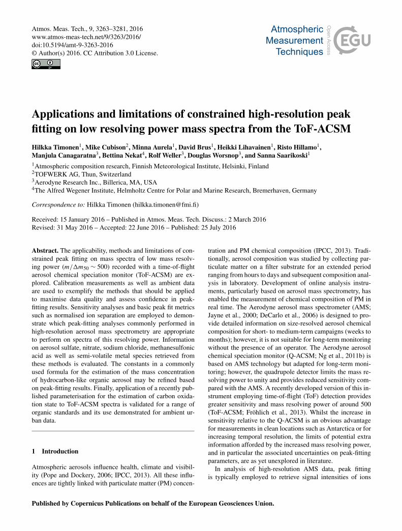
Table 1. Mass accuracy in ppm obtained using the true and compen-sated exact masses for the tungsten ions during mass calibration.
Ion SF+3 SF+4 SF+5
Using true W+ m/Q −71 −21 −76Compensated −57 −3 −53
mass excess are used in Eq. 1 to calculate the correspond-ing position of the tungsten (calibrant) ions. Figure S6 exem-plifies this approach. The surrounding isobaric peaks havean average mass excess of 0.095 Th and intensity of 665 ions(∼ 15 times smaller than the tungsten peaks), leading to smallpositive shifts to the estimated “true” mass positions of thetungsten ions of ∼ 0.006 Th (35 ppm).
In this example, the compensation for the influencingpeaks would be applied in the mass calibration by enteringnot the true tungsten isotope exact masses (red circles inFig. S6) but rather these values less the 35 ppm offset cal-culated above (yellow circles). To assess the validity of thismethod, the mass spectrum used in the example was recordedusing a calibration gas SF6 injected at the ioniser, giving riseto strong signals at the nominal masses 89, 108 and 127 Thfrom the ions SF+3 , SF4+ and SF+5 respectively. The masscalibration was performed based on the air peaks and thetrue or compensated tungsten peaks, and the mass offset ofthe SF+3 , SF+4 and SF+5 peaks calculated. As shown in Ta-ble 1, the mass accuracy was improved by ∼ 20 ppm usingthe compensation technique described here.
For the example MS used in these calculations, the tung-sten ion peaks were∼ 15 times stronger than the surroundingpeaks which we will refer to here as “background”, that is,the signal at the mass to charge ratios surrounding the cali-brant ion signal. Assuming the same background peaks werepresent, but exhibited different intensities relative to the tung-sten peaks, Fig. 4 shows the estimated relative compensationthat would be applied. For a W+/ background ratios of 100,a relative compensation of only 4 ppm is expected and thistechnique would have almost negligible effect on peak fittingat the mass resolving power of the ToF-ACSM. However, fora W+/ background ratio of 5 (as may be expected in dirtyenvironments), the relative compensation exceeds 100 ppmand use of the technique would need to be treated with theappropriate caution.
3.2.3 Alternative background peaks to tungsten ions
For datasets where the use of the tungsten ions in the masscalibration is not acceptable, an alternative constraint on theupper part of the MS is desired.
Trichloroethylene
We propose that the fragmentation pattern from the industrialsolvent trichloroethylene is a potentially useful candidate for
500
400
300
200
100
0
ppm
com
pens
atio
n
12 3 4 5 6 7 8
102 3 4 5 6 7 8
100
Ratio signals W+ / background
Figure 4. Estimated relative compensation that would need to beapplied to the W+ exact mass owing to an influencing, overlap-ping, background peak separated by 0.095 Th and of relative signalstrength indicated by the x axis.
ToF-ACSM (and AMS) mass calibration. Isotope patternsmatching the NIST EI reference MS for trichloroethyleneare apparent in multiple ToF-ACSM and AMS datasets. Inparticular, MS peaks which appear to correspond to the ionsC35
2 Cl3H+ and C372 Cl35Cl2H+ at the nominal masses 130 and
132 Th, respectively, are often visible in ToF-ACSM massspectra recorded in clean locations with low background. Thetime trend of the peak intensities for these ions follows that ofthe sensitivity of the instrument, indicating that the source ofthe interference lies within the vacuum chamber, most likelyin the ionisation region. The peaks do not show up in the dif-ference spectra and it is unlikely that trichloroethylene gasmolecules from an external source could sufficiently pen-etrate the differential pumping system, which dilutes back-ground gas molecule concentrations by a factor of 107.
The identification of the isotope pattern at 130, 132 and134 Th as trichloroethylene is supported by data from theHR-ToF-AMS. Figure 5 shows a HR-ToF-AMS MS recordedat the urban station in Helsinki (Mäkelänkatu) alongside aToF-ACSM MS from the Neumayer station. Applying free-position peak fits as in Sect. 3.2.2 gave fitted peak positionsdeviating from those of the trichloroethylene ions of 0.2,−4.6 and 3.2 ppm in the HR-ToF-AMS (limited by countingstatistics) and 0.9, 4.9 and 109 ppm in the ToF-ACSM MS for130, 132 and 134 Th respectively. Whilst the trichloroethy-lene ions are clearly well separated from their neighbours bythe HR-ToF-AMS, this is not the case for the ToF-ACSMand thus for calibration purposes the Trichloroethylene ionsignals must, as was already pointed out for use of the tung-sten ions, be significantly larger than the background in or-der to be considered as reliable mass calibration peaks. Inthe Neumayer dataset, the C35
2 Cl3H+ and C372 Cl35Cl2H+ sig-
nals were roughly 30 times larger than the background sig-nal. The influence of the background ions is thus small and arelative centroid position shift of only 4 ppm is observed. Acompensation of the exact masses during calibration as de-scribed above would thus have negligible effect. The sameis not true for the weaker C37
2 Cl352 ClH+ ion, whose centroid
www.atmos-meas-tech.net/9/3263/2016/ Atmos. Meas. Tech., 9, 3263–3281, 2016

3270 H. Timonen et al.: Constrained peak fitting of ToF-ACSM data
134132130128
Nor
mal
ised
sig
nal
Nor
mal
ised
sig
nal
ToF-ACSM (ETOF)
HR-ToF-AMS (HTOF)
Trichloroethylene isotope pattern Mass spectra (data)
m Q (Th)-1
Figure 5. Mass spectra from the ToF-ACSM and HR-ToF-AMSshowing the isotope pattern of trichloroethylene (C2Cl3H+).
position is shifted relative to the stronger isotope peaks byover 100 ppm.
For the Neumayer data, trichloroethylene proved to be amuch more useful constraint on the upper region of the masscalibration than the tungsten ions, whose signal relative tobackground was an order of magnitude weaker. Nonethe-less, it is important to note that the peaks do not representtruly isolated ions, as is clearly visible when comparing theHR-ToF-AMS and ToF-ACSM spectra in Fig. 5. Calibrationbiases of order a few ppm can be expected as a result andshould be considered when assessing peak-fitting results, aswill be discussed later.
Extrapolation
In the absence of a valid constraint on the upper region ofthe mass calibration, the question is posed as to whether it isbetter to utilise the poorly defined calibrant peak regardlessor simply extrapolate the calibration from the lower, well-defined, region of the MS. To investigate this, lab data wererecorded where SF6 gas was injected directly into the ion-isation region, leading to strong signals at unit masses 89,108 and 127 Th from the ions SF+3 , SF+4 and SF+5 respec-tively. A mass calibration was performed using the square-root relationship ToF= a+ b×
√(m/Q) and the calibrant
peaks OH+, N+2 , O+2 , Ar+ and CO+2 . The offsets from thetrue peak positions for SF+3 and SF+4 were then assessedfor the extrapolated calibration and again when additionallyusing SF+5 as a calibrant peak. For the constrained calibra-tion (with SF+5 ), offsets of −31 and 25 ppm were found forSF+3 and SF+4 respectively. Without the SF+5 constraint, thesechanged to−71 and−19 ppm respectively, a difference of upto approximately −40 ppm. In Sect. 3.2.2 it was shown howinterferences around the tungsten ions could lead to centroidpeak position shifts of > 100 ppm, indicating that an extrapo-lated calibration could indeed be preferred over introductionof a bias of unknown direction and magnitude due to inter-ferences at the calibrant peaks.
It is noted that the offsets (biases) of a few tens of ppmrepresent the limiting average mass accuracy across the MSrange that may be expected during routine ToF-ACSM op-eration. Careful calibrant selection, fitting of a sub-rangeand/or use of more complicated ToF/mass relationships mayincrease accuracy to below 10 ppm, but during normal opera-tion the user should expect mass axis biases of around 10–20and 50–100 ppm in the lower and upper regions of the MSrespectively. Fitted peak intensities should be evaluated ac-cordingly (see Corbin et al., 2015, for a detailed discussionon the influence of calibration bias on fitted peak intensity).
Addition of calibrant compounds
In the HR-ToF-AMS, the use of a plastic servomotor insidethe vacuum chamber leads to a background peak at 149 Thfrom the ionisation of the phthalate molecules leaching outfrom the plastic. This is a useful and commonly used cal-ibrant peak that is, however, missing from the ToF-ACSMMS, as the instrument does not utilise this particular compo-nent. In the Q-ACSM, a naphthalene source is intentionallyinstalled in the ioniser region to generate known backgroundpeaks for both transmission correction and mass calibration.In the interest of securing a decent calibration, installationin the vacuum chamber of a naphthalene source or a simpleplastic element known to release phthalates into the environ-ment could be a useful future modification to the instrument.
3.3 Peak-fitting uncertainties and terminology
Cubison and Jimenez (2015) give parameterisations to es-timate the precision, σI, on fitted peak intensity for a sys-tem of two overlapping peaks using the same constrainedpeak-fitting procedure employed in this study. The two de-pendent parameters are the ratio of the two peak intensities,RI, and the peak separation normalised to half-width at half-maximum (HWHM), X. As RI increases, the precision withwhich the intensity of the less-intense ion peak can be fit-ted degrades. As X decreases, the same is true for both themore- and less-intense peaks. As a general rule, for RI up to∼ 10, the fitted intensity of the child peak can be retrievedwith acceptable precision for X as low as ∼ 0.7. For smallerX, the imprecision increases and obtaining reliable resultsbecomes challenging and eventually impossible. Peaks sepa-rated by X> 1.6 can nearly always be reliably fitted, exceptin the case of RI> 200, above which the imprecision on thefitted parameters of the less-intense peak is so great as topreclude their use in data analysis. It is noted that Cubisonand Jimenez (2015) assumed a constant peak shape in deriv-ing this parameterisation, which thus represents the best-casescenario and should be interpreted accordingly. We make useof this parameterisation in this study when discussing peakseparations, which we state henceforth as X, i.e. normalisedto HWHM.
Atmos. Meas. Tech., 9, 3263–3281, 2016 www.atmos-meas-tech.net/9/3263/2016/

H. Timonen et al.: Constrained peak fitting of ToF-ACSM data 3271
4 Results and discussion
4.1 Ammonium
Data collected at the urban background station, SMEAR III,are used to study fitting of main inorganic ions, ammonium,nitrate and sulfate. Peak fitting is routinely used on HR-ToF-AMS spectra to determine ammonium signal intensities, asNH+2 , NH+3 and NH+4 all have large isobaric interferences(from O+, HO+ and H2O+ respectively) and the integrateddata time series, constructed based on molecular fragmenta-tion patterns which account for these large interferences (Al-lan et al., 2004), are thus noisy and detection limits corre-spondingly high. Fröhlich et al. (2013) applied peak fittingto ToF-ACSM spectra and concluded that the NHx ions wereunresolvable from the interfering ions; we extend this dis-cussion, with reference to the peak separations and expectedintensity ratios, as the NHx ions exemplify how the intensi-ties of well-separated peaks cannot always be accurately fit-ted. In the case of NH+2 , NH+3 and NH+4 , X approaches unityand the peaks can be considered partially separated. How-ever, for peak ratios over 100 as are observed for these ions,X > 1 is required even to achieve precisions on fitted inten-sity, σI, of 100 % (Cubison and Jimenez, 2015), effectivelyprecluding successful peak fitting for all but the strongestammonium signals. The only possibility for extracting use-ful information on ammonium from peak fitting is thus at15 Th where the interferences on NH+ are much smaller, asexemplified in Fig. 6. However, with peak separations to theneighbouring ions of X = 0.5, the imprecision expected inthe fits is still large. Batch peak fitting at 15 Th on ammo-nium nitrate calibration data yielded a time series for NH+
whose signal : noise was similar to that of the integrated peaktime series. However, peak fitting did not improve the qualityof the data and thus for ammonium could only be used to helpsupport assumptions required to construct the integrated datafragmentation table. It is estimated that mass resolving powerapproaching 1000 in this lower region of the MS would berequired in order to reliably deconvolve the ammonium peakintensities.
4.2 Nitrate
In AMS analysis, concentrations of aerosol species fromintegrated unit-mass data are calculated based on well-described fragmentation patterns (Allan et al., 2004). Previ-ous studies have shown that, in many ambient conditions,the default fragmentation patterns work well. However, inthe case of high organic loadings and particularly duringbiomass-burning events, the assumptions tend to break downand nonsensical mass concentrations may result (e.g. Ortegaet al., 2013). In general, it is preferred to construct the timeseries from the sum of individual fitted ion intensities, pro-viding of course that the uncertainty on these values is notlarge.
1500
1000
500
0
15.1515.1015.0515.0014.9514.90
15
N +
NH +
CH3 +
Ions
m Q (Th)-1
Figure 6. The isobaric peaks 15N+ (m/Q= 14.9996 Th), NH+
(m/Q= 15.01035 Th) and CH+3 (m/Q= 15.0229 Th) at 15 Thhave peak separations of 0.5 half-widths for mass resolving powerm/1m= 300.
Inorganic nitrate is an important aerosol component whoseprincipal contributing ion signals, NO+ and NO+2 , both suf-fer from isobaric interferences due to neighbouring organicions. Although Fröhlich et al. (2013) reported that it shouldbe possible to use peak fitting to resolve these interferences,the peak separations are very small indeed and no uncertain-ties or confidence metrics were presented. We address theseissues here in detail.
At 30 Th the peak separations of NO+ from the organicisobaric interferences CH2O+ and C2H+6 areX ∼ 0.3 and 1.3respectively (Fig. 7). A similar situation presents itself forNO+2 at 46 Th (isobaric ions CH2O+2 and C2H6O+). Calcu-lating peak intensity via peak fitting on fixed-position peaksseparated by X ∼ 0.3 is extremely sensitive to the mass cali-bration. However, fortuitously in this case, the isobars 30 and46 Th both lie close to calibrant ions used in the mass cali-bration; in the case of 30 Th the isobar is surrounded by N+2at 28 and O+2 at 32 Th. As a result, the bias expected in thecalibration is very small relative to other regions in the massspectrum (where the calibration may be extrapolated) and itsmagnitude can be predicted from the biases of the calibrantions themselves.
Given the expected sensitivity of the highly overlappingfits to the mass calibration, it is appropriate to conduct asensitivity analysis to assess the degree of confidence thatmight be drawn from the fitted intensity values. Tofware of-fers a graphical tool for this purpose. An example is given forthe isobar 30 Th, with fitted ions NO+, CH2O+ and C2H+6 ,in Fig. 8, using data from the SMEAR III campaign. Usingthe ions H2O+, N+2 , O+2 and CO+2 to perform the mass cali-bration gave mass accuracies of between 2 and 13 ppm. As-sessment of the sensitivity of the fitted intensities at 30 Thto mass calibration bias does not therefore need to con-sider much larger values than this; we conservatively chose20 ppm, which equates to about 5 % of the separation of theions NO+ and CH2O+. In the general case, a larger perturba-
www.atmos-meas-tech.net/9/3263/2016/ Atmos. Meas. Tech., 9, 3263–3281, 2016
3272 H. Timonen et al.: Constrained peak fitting of ToF-ACSM data
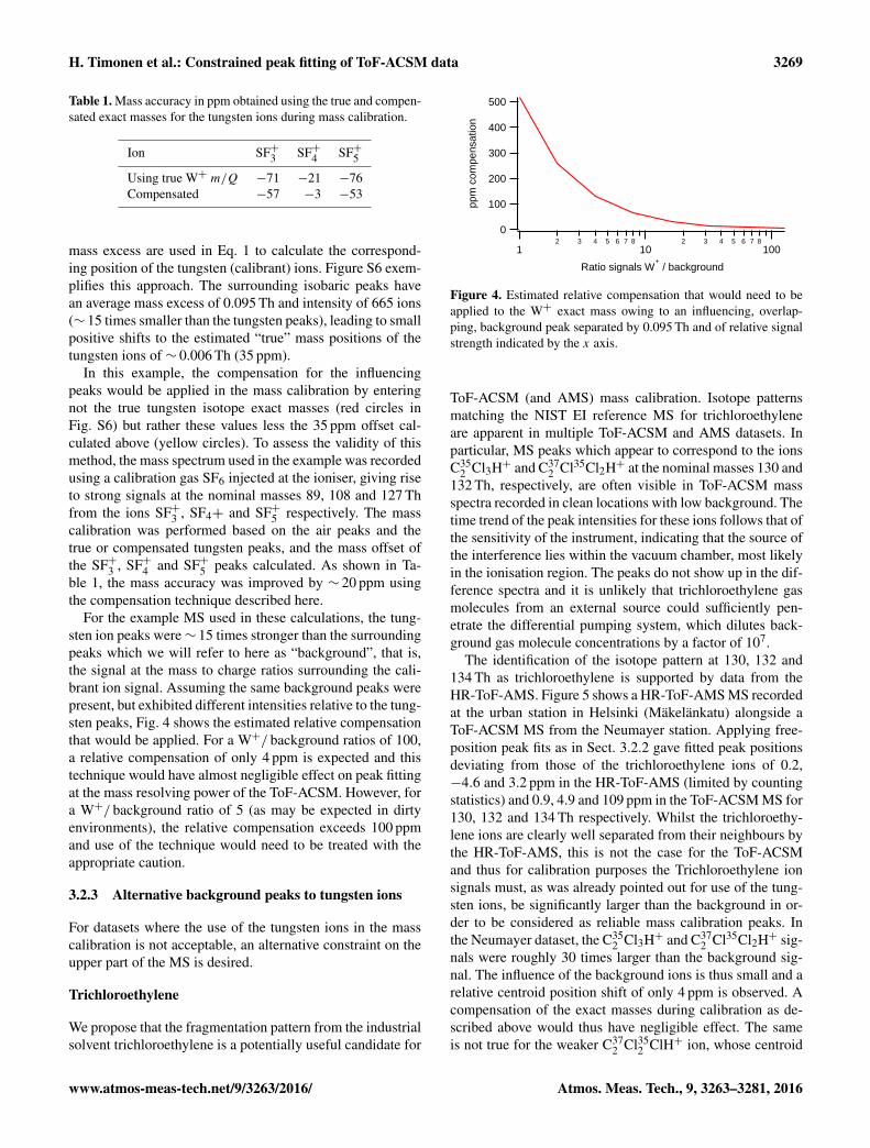
Figure 7. The isobaric peaks from NO+ (m/Q= 29.997 Th) andCH2O+ (m/Q= 30.010 Th) at 30 Th have a peak separation of 0.34half-widths for resolving power m/1m= 400.
-8
-4
0
4
8
9:30 9:45 10:00 10:15 10:30 10:45 11:00
Time
-4
-2
0
1000
800
600
400
200
0
Pert
urb
ed
fit
ted
in
ten
sity
10008006004002000
Fitted intensity (ions/s)
9:30 9:45 10:00 10:15 10:30 10:45 11:00
Time
1000
800
600
400
200
0
Fitt
ed
in
ten
sity
(io
ns/
s)
1000
800
600
400
200
0
"Actual" time-series
Positively-perturbed mass cal.
Negatively-perturbed mass cal.
Precision estimate from
Cubison & Jimenez 2015
Integrated intensity ("unit-mass")
NO+ (88.3 %) CH2O+ (5.0 %)
C2H6+ (6.8 %)
Pos. fit: y = 4.49 + 1.05 * x
Neg. fit: y = -1.10 + 0.90 * x
Abs.
resi
d. (i
ons
s )-1
Inte
nsity
(ion
s s
)-1%
resi
d.
Figure 8. Assessing the sensitivity of the fitted peak intensity ofthe NO+ ion as a function of time to perturbations in the mass cal-ibration of ±20 ppm. Left: the sum of the ions fitted at this peakcompared with the integrated signal (bottom) and the absolute andrelative residuals (top). Top right: scatter plots of the fitted NO+
signals for the perturbed vs. best-case mass calibration scenarios.Bottom right: time series of the fitted NO+ intensities, with the per-turbed mass calibration cases shown in red and blue. The shadingaround the black line indicates the expected precision predicted bythe parameterisation of Cubison and Jimenez (2015).
tion value of between 50 and 100 ppm would be appropriate,depending on the confidence in the calibration.
From Fig. 8 one can take confidence that the fitted NO+
ion intensities are reliable. Firstly, consider the time seriesof the fitted vs. integrated peak intensities and their residualsfor the unperturbed mass calibration (left panels). The sumof the fitted peak intensities matches the integrated values towithin a few percent (Figs. 8 and S7). For 20 s averaging ofa peak with a significant non-zero MS baseline and closely
separated neighbouring isobaric peaks (which influence theintegrated intensities), this level of agreement is indeed in-dicative that the peak-fitting process has been properly per-formed. The step changes in the summed fitted intensity asthe aerosol filter is switched in/out of the inlet line are alsoaccurately captured.
The influence of perturbing the mass calibration is shownin the right panels as a time series (bottom) and scatter plot(top). When positively perturbing the calibration by 20 ppm(shifting the entire mass axis 20 ppm= 30 Th×20/1×106= 0.0006 Th but holding peak positions fixed), the fitted
NO+ intensity increases by 10 %. A negative perturbation ofsimilar magnitude would decrease fitted intensity by 12 %. Itis important to note that this is a sensitivity analysis and notan uncertainty calculation on the fitted intensities; nonethe-less the method does offer a useful validity check on the fittedparameters. We henceforth refer to the relative intensity bias(offset, in percent) introduced by calibration perturbation as1I.
Regarding the perturbed time series, the estimated preci-sion on fitted intensity from the parameterisation of Cubisonand Jimenez (2015), σI, is also shown on the unperturbed in-tensity time series (shaded area, bottom right panel). The fit-ted intensity of the NO+ ion is deconvolved with σI less thana few percent. Although this example presents a truly chal-lenging peak-fitting scenario with limited signal and a largedegree of peak overlap, one may draw conclusions based onthe actual fitted peak intensities provided they held true forchanges of roughly ±10 %. Similar conclusions may also bedrawn looking at NO+2 at 46 Th (Fig. S8).
It is noted that this assessment of the uncertainties assumesan invariant and correctly defined peak shape. Inaccuracies inthe peak shape arising from either instrumental artefacts oruser error in its definition would propagate into errors in thefitted intensities discussed above. Although a quantitative as-sessment of these effects is outside of the scope of this study,we illustrate the impact of an incorrect peak shape by com-paring the fit results for NO+ and its interferences using theuser-defined and Gaussian peak shapes. For a representativeMS from the SMEAR dataset, we observe that 73 % of thearea is assigned to the NO+ ion using peak fitting with theuser-defined shape. Using Gaussians, this increases to 87 %,a relative change of+19 %. Whilst such a large inaccuracy inpeak shape would not be expected (and indeed the fit resid-uals are large and apparent using Gaussians), this highlightsthe importance of carefully defining the peak shape as de-scribed in Sect. 3.1.2.
Finally, it is noted that, for the data shown, the organicmass loading was approx. 1.5 times that of the nitrate. Inspectra with large organic signals, the relative strength of thenitrate ions to the organic interferences would be smaller andthe corresponding uncertainty larger. Nonetheless, the samemethodology presented here could be applied to assess theuncertainties.
Atmos. Meas. Tech., 9, 3263–3281, 2016 www.atmos-meas-tech.net/9/3263/2016/

H. Timonen et al.: Constrained peak fitting of ToF-ACSM data 3273
1000
800
600
400
200
0
Ions
s
2.3.2014 3.3.2014 4.3.2014 5.3.2014 6.3.2014 7.3.2014 8.3.2014
160
140
120
100
80
60
40
20
0
Ions
s
Integrated data, SO+,
SO2+, SO3
+, H2SO4
+,
HSO3+
C4+ C6H8
+ C6H10O
+C5H4O
+
C5H5O+ C5H5O2
+ CH4O2
+
C5H5O2+ C5H5O2
+ C5H5O2
+
-1-1
Figure 9. Concentrations of main sulfate ions (SO+, SO+2 , SO+3 ,HSO+3 and H2SO+4 ) from peak fitting and sulfate calculated fromapplication of the fragmentation table with integrated data (lowerpanel) and time series of the isobaric organic ions in the same m/Qas sulfate fragments (upper panel).
4.3 Sulfate
Sulfate is a further important inorganic aerosol componentmeasured by the ToF-ACSM. The principal contributingions, SO+, SO+2 , SO+3 , HSO+3 and H2SO+4 , are all affectedby isobaric organic influences and the total sulfate concen-tration from integrated peak data over the nominal massesis, as per ammonium and nitrate, calculated based on as-sumed fragmentation patterns to account for these influences(henceforth referred to simply as “integrated data”). Like ni-trate, these assumptions tend to break down for high organicmass loading and particularly for biomass burning. However,with X values relative to the closest organic interferencesof 0.5–0.8, constrained peak fitting can be employed to di-rectly calculate the sulfate ion signals with acceptable un-certainty. To demonstrate this, peak fitting was performed onthe SMEAR III dataset and an analogous sensitivity analysiswas performed as presented for nitrate in the previous sec-tion (Figs. S9–S13). The mass calibration perturbation em-ployed for these sensitivity analyses reflected the position ofthe ions under study in the mass spectrum, relative to thoseused to perform the calibration (H2O+, N+2 , O+2 and CO+2 ).Thus, the confidence in the mass calibration at 48 Th (SO+)is quite high and a 20 ppm perturbation was applied. In con-trast at 98 Th (H2SO+4 ), the calibration is somewhat extrapo-lated and a 50 ppm perturbation was applied. An example ofperturbed time series for SO+ ion is in Fig. S14. The result-ing sensitivities of the fitted intensities to calibration pertur-bations, 1I, ranged from approx. 3 to 30 %.
The SMEAR III data are used to demonstrate constructionof a mass-loading time series for sulfate based on the sum ofthe sulfate ion signals retrieved from peak fitting (Fig. 9). Thesum of the fitted intensities was able to reconstruct the sametime series as that from the fragmentation table with only 3 %difference (integrated ∼ 1.03×fitted), demonstrating the va-lidity of the method. Figure 9 shows the fitted intensities of
the isobaric interferences from organic ions. The ratio of theorganic signal from the integrated data to the sum of the fit-ted intensities of the organic ions is 0.64± 0.40. Overall, thepeak-fitting method weighted the allocation of the ion sig-nals more heavily towards organic than the fragmentationtable approach. However, the differences are small and theonly significant conclusion that may be drawn is that, for thisdataset, the methods are consistent for a sulfate to within afew percent.
4.4 Sodium chloride
The Neumayer station, situated in a clean environment adja-cent to the open ocean, provides an ideal location to studycompounds originating from the sea. Data collected on Neu-mayer station were used to study peak fitting of sodium, chlo-ride and methanesulfonic acid. The mass calibration for theNeumayer dataset was performed using the following cali-brant ions; H2O+, N+2 , O+2 , Ar+, CO+2 , SO+2 , C35
2 Cl3H+ andC35
2 Cl372 ClH+. The isolated ion peak shape was used rather
than a Gaussian to optimise the calibrant ion fits. Mass accu-racy was in the range 10–20 ppm for all calibrant ions.
On 2 and 3 December 2014, elevated aerosol chloridewas observed at the Neumayer station (Figs. S15–S16). Air-mass back trajectories (Global Data Assimilation System(GDAS) data, NOAA Hybrid Single-Particle Lagrangian In-tegrated Trajectory model (HYSPLIT, v4.9); Draxler andRolph, 2013) show that the air mass was transported alongthe Antarctic coastline at low altitudes during the previousdays, pointing to the influence of sea salt as an explanationfor the observed chloride concentrations of up to 300 ng m−3
(Fig. S15). Neither MSA, proxied by m/Q 79, nor organicaerosol was elevated during this period. Peak fitting was con-ducted on the mass spectra from this episode to (i) demon-strate the presence of sea-salt-related compounds and (ii)generate a time series for NaCl+, separated from its isobaricorganic interference(s). The chloride ions 35Cl+ and 37Cl+
have only relatively tiny interferences in ToF-ACSM massspectra and thus no meaningful additional information canbe expected to be gained from peak fitting relative to the in-tegrated peak data, except perhaps in exceptionally large or-ganic plume cases.
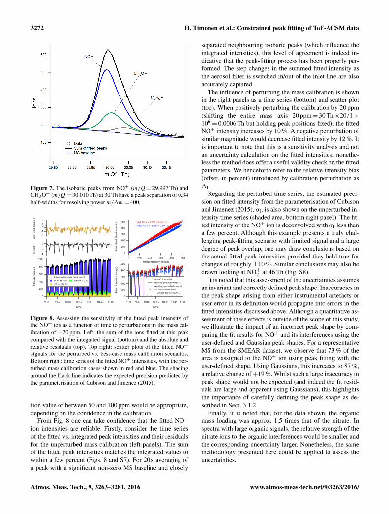
Several ions attributable to sea salt (following Schmaleet al., 2013.), such as Na35Cl+ (57.958 Th), Na37Cl+
(59.956 Th), Fe35Cl+2 (125.87 Th) and Fe37Cl35Cl+
(127.87 Th), could be identified in the average mass spec-trum from this period, as shown in Fig. 10. In the case ofNaCl+, three interfering isobaric organic ions are knownto be visible in ToF-ACSM mass spectra; at this massresolving power it is not possible to state which of these areobserved here, although the oxygenated peak C3H6O+ is alikely candidate and is demonstrated in Fig. 10. However,irrespective of the interference(s) chosen, sensitivity of thefitted intensity of NaCl+ to a 100 ppm mass calibrationperturbation was ∼ 5 %, indicating that the majority of the
www.atmos-meas-tech.net/9/3263/2016/ Atmos. Meas. Tech., 9, 3263–3281, 2016
3274 H. Timonen et al.: Constrained peak fitting of ToF-ACSM data
m Q (Th)-1
m Q (Th)-1
m Q (Th)-1
Figure 10. Top: Isobaric peaks of NaCl+ and C3H6O+. Centre:total mass spectrum showing the calibrant ion C2Cl3H+ and sig-nals from unknown compounds at nominal masses 126 and 128 Th.Bottom: difference mass spectrum (ambient minus filter) show-ing statistically relevant signals from the isotopes Fe35Cl+2 andFe37Cl35Cl+.
difference signal at 58 Th could indeed be attributed to thision.
The FeCl+ ions are shown as a further example of seasalt compounds that could be unambiguously identified inthe Neumayer data. The centre panel in Fig. 10 shows a por-tion of the average total mass spectrum together with peak-fitting curves for the period during which elevated chloridewas observed. The mass calibrant ion C2Cl3H+ at 130 This visible in addition to unknown background ion(s) at 126and 128 Th. For the difference mass spectrum, however,these background ions contribute only to the noise and twoaerosol signals are resolvable above the noise level, definedas 3 times the standard deviation over the adjacent massrange. These signals are well represented by the Fe35Cl+2and Fe37Cl35Cl+ isotopes; the mass excess of these aerosolpeaks is significantly (∼ 1500 ppm) less than the backgroundpeaks observed for the total mass spectrum. We note that itis almost certain that the signal from a multitude of unre-solvable organic ions combines together to give the appar-ent single background peak, but in this analysis we are onlyconcerned with the relatively well-separated sea salt signals.Further support to their identification is given by the ratio ofthe signal intensities. 37Cl exhibits only 32 % the abundanceof the 35Cl isotope, and thus an intensity ratio of 67 % is ex-
2000
1500
1000
500
0
-500
Fit
ted
in
ten
sity
(to
tal
ion
co
un
ts)
0:00
3.12.2014
0:00
4.12.2014
0:00
5.12.2014
400
300
200
100
0
-100
-200
Na
Cl + in
ten
sity (to
tal io
n co
un
ts)
80006000400020000
Cl+ intensity (total ion counts)
y = 0.04 x + 28
R2 = 0.4
NaCl+
C3H6O+
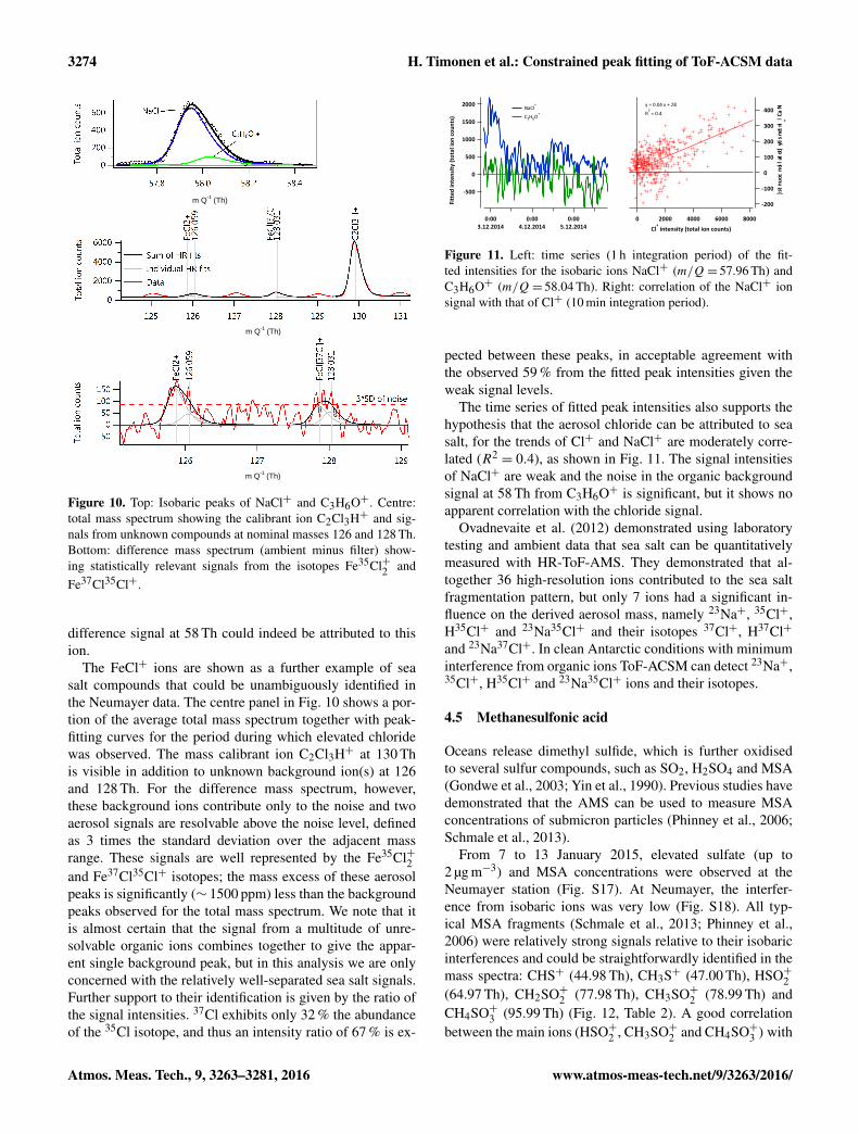
Figure 11. Left: time series (1 h integration period) of the fit-ted intensities for the isobaric ions NaCl+ (m/Q= 57.96 Th) andC3H6O+ (m/Q= 58.04 Th). Right: correlation of the NaCl+ ionsignal with that of Cl+ (10 min integration period).
pected between these peaks, in acceptable agreement withthe observed 59 % from the fitted peak intensities given theweak signal levels.
The time series of fitted peak intensities also supports thehypothesis that the aerosol chloride can be attributed to seasalt, for the trends of Cl+ and NaCl+ are moderately corre-lated (R2
= 0.4), as shown in Fig. 11. The signal intensitiesof NaCl+ are weak and the noise in the organic backgroundsignal at 58 Th from C3H6O+ is significant, but it shows noapparent correlation with the chloride signal.
Ovadnevaite et al. (2012) demonstrated using laboratorytesting and ambient data that sea salt can be quantitativelymeasured with HR-ToF-AMS. They demonstrated that al-together 36 high-resolution ions contributed to the sea saltfragmentation pattern, but only 7 ions had a significant in-fluence on the derived aerosol mass, namely 23Na+, 35Cl+,H35Cl+ and 23Na35Cl+ and their isotopes 37Cl+, H37Cl+
and 23Na37Cl+. In clean Antarctic conditions with minimuminterference from organic ions ToF-ACSM can detect 23Na+,35Cl+, H35Cl+ and 23Na35Cl+ ions and their isotopes.
4.5 Methanesulfonic acid
Oceans release dimethyl sulfide, which is further oxidisedto several sulfur compounds, such as SO2, H2SO4 and MSA(Gondwe et al., 2003; Yin et al., 1990). Previous studies havedemonstrated that the AMS can be used to measure MSAconcentrations of submicron particles (Phinney et al., 2006;Schmale et al., 2013).
From 7 to 13 January 2015, elevated sulfate (up to2 µg m−3) and MSA concentrations were observed at theNeumayer station (Fig. S17). At Neumayer, the interfer-ence from isobaric ions was very low (Fig. S18). All typ-ical MSA fragments (Schmale et al., 2013; Phinney et al.,2006) were relatively strong signals relative to their isobaricinterferences and could be straightforwardly identified in themass spectra: CHS+ (44.98 Th), CH3S+ (47.00 Th), HSO+2(64.97 Th), CH2SO+2 (77.98 Th), CH3SO+2 (78.99 Th) andCH4SO+3 (95.99 Th) (Fig. 12, Table 2). A good correlationbetween the main ions (HSO+2 , CH3SO+2 and CH4SO+3 )with
Atmos. Meas. Tech., 9, 3263–3281, 2016 www.atmos-meas-tech.net/9/3263/2016/

H. Timonen et al.: Constrained peak fitting of ToF-ACSM data 3275
10
8
6
4
2
0
Ions
s
7.1.15 8.1.15 9.1.15 10.1.15 11.1.15 12.1.15 13.1.15
CHS+, CH3S
+, HSO2
+
CH2SO2+, CH3SO2
+ CH4SO3
+,
-1
Figure 12. Time series of MSA fragments CHS+ (44.98 Th),CH3S+ (47.00 Th), HSO+2 (64.97 Th), CH2SO+2 (77.98 Th),CH3SO+2 (78.99 Th) and CH4SO+3 (95.99 Th) during episode 2.
Table 2. Observed MSA ions, their principal isobaric ions and peakseparation
Ion m/Q (Th) Principal isobaric Peakions separation X
CHS+ 44.979347 C2H5O+, 13CO2 0.2CH3S+ 46.994999 CH3O+2 , CCl+ 0.3HSO+2 64.969177 C4HO+, C5H+5 0.4CH2SO+2 77.977005 C5H2O+, C6H+6 0.3CH3SO+2 78.984825 C5H3O+, C6H+7 0.3CH4SO+3 95.987564 SO+4 0.2
highest signals was observed (Fig. S19, Table S1). However,we note that for all MSA ions the separation from isobaricions was low (X = 0.2–0.4), thus increasing the uncertainlyof the results. In typical conditions with larger backgroundand/or organic signals, this analysis would become difficultand uncertainties large. In clean conditions ToF-ACSM pro-vided the possibility to discern between and measure bothsulfate and MSA fragments, which combined with meteoro-logical data could be used to e.g. further study the CLAWhypothesis (Charlson et al., 1987).
4.6 Metals
Data collected in an underground mine are used to study thepeak fitting of ions from semi-volatile metals. It has beendemonstrated that the ToF-AMS, upon whose technologythe ACSM is based, is capable of detecting ions associatedwith the metals Cu, Zn, As, Se, Sn and Sb (Salcedo et al.,2012). Further semi-volatile elements may also be measur-able based on their melting or thermal decomposition points(Drewnick et al., 2015). In the mine environment it is ex-pected that metallic elements comprise a significant fractionof the aerosol mass (Csavina et al., 2012). The undergroundmine dataset is thus a good example of a first assessment ofthe capability of the ToF-ACSM to detect metal species. Theions of these species tend to have large mass excesses and areoften separated from their neighbouring ions by X> 1, indi-cating that peak fitting should be able to resolve their signals.
Table 3. Peak separation X, normalised to HWHM, of various met-als ions from neighbouring ions for instrumental mass resolvingpower of m/1m= 450.
Peak separation X fromElement Ion closest neighbouring ion
(normalised to HWHM)
As 75As+, 75As+2 1.0
Cu 63Cu+ 1.065Cu+ 1.2
Sb 121Sb+ 1.2123Sb+ 1.0
Se 74Se+ 1.276Se+, 77Se+ 0.978Se+ 1.180Se+ 0.1
Sn 116Sn+, 118Sn+ 1.1120Sn+ 1.5
Zn 64Zn+ 0.466Zn+, 67Zn+, 68Zn+ 1.270Zn+ 1.5
These peak separations are given in Table 3 for the isotopesof the metals reported detectable by Salcedo et al. (2012).
High signal levels, such as those observed in the mine (upto 200 µg m−3), clearly improve peak fitting, as the descrip-tion of the peak shape is well defined by the discrete datapoints with high signal : noise ratio. However, the multipleinterferences at nearly every isobar precludes a truly accu-rate mass calibration and certain assumptions must be madewhen performing this analysis step. Consequently, a carefulsensitivity analysis must be performed before drawing con-clusions from the fitted peak intensities. To highlight the per-formance of the instrument and fitting procedure in measur-ing changes in mass component intensities, a period at theend of a working day was chosen for detailed analysis, whenthe organic mass loading in the mine falls sharply from > 30to < 3 µg m−3 over a 2 h period.
As many of the metals isotopes exhibit mass excesses thatdiffer significantly from other (in most cases organic) peaksin the MS, representation of the fitted position in m/Q ofeach isobaric peak in a mass excess plot can be used to high-light features of interest, as shown in Fig. 13. Certain peaksstand out from the general pattern as having mass excessesthat deviate from the general trend, principally those fromSOx (48, 64, 66) and Asx (75, 150). It is noted that there isa contribution from 66Zn+ at 66 Th which also contributes tothe observed negative mass excess. A more detailed investi-gation was thus undertaken to assess potential signals fromthe As and Zn ions.
www.atmos-meas-tech.net/9/3263/2016/ Atmos. Meas. Tech., 9, 3263–3281, 2016
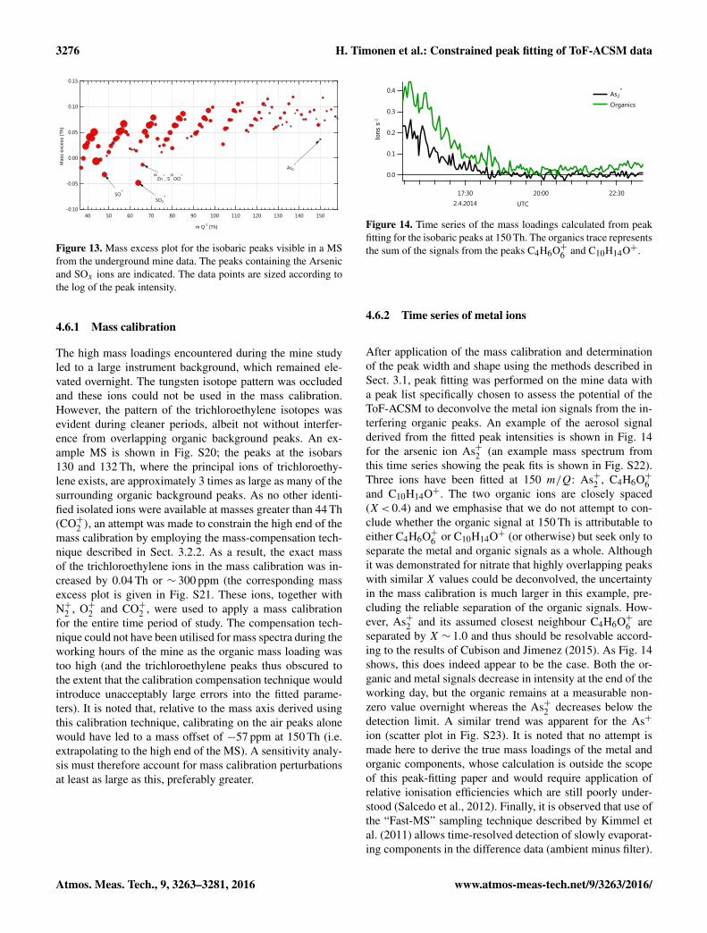
3276 H. Timonen et al.: Constrained peak fitting of ToF-ACSM data
0.15
0.10
0.05
0.00
-0.05
-0.10150140130120110100908070605040
SO+
SO2
+
66
Zn+
, S18
OO+
As2
+Mas
s ex
cess
(Th)
m Q (Th)-1
Figure 13. Mass excess plot for the isobaric peaks visible in a MSfrom the underground mine data. The peaks containing the Arsenicand SOx ions are indicated. The data points are sized according tothe log of the peak intensity.
4.6.1 Mass calibration
The high mass loadings encountered during the mine studyled to a large instrument background, which remained ele-vated overnight. The tungsten isotope pattern was occludedand these ions could not be used in the mass calibration.However, the pattern of the trichloroethylene isotopes wasevident during cleaner periods, albeit not without interfer-ence from overlapping organic background peaks. An ex-ample MS is shown in Fig. S20; the peaks at the isobars130 and 132 Th, where the principal ions of trichloroethy-lene exists, are approximately 3 times as large as many of thesurrounding organic background peaks. As no other identi-fied isolated ions were available at masses greater than 44 Th(CO+2 ), an attempt was made to constrain the high end of themass calibration by employing the mass-compensation tech-nique described in Sect. 3.2.2. As a result, the exact massof the trichloroethylene ions in the mass calibration was in-creased by 0.04 Th or ∼ 300 ppm (the corresponding massexcess plot is given in Fig. S21. These ions, together withN+2 , O+2 and CO+2 , were used to apply a mass calibrationfor the entire time period of study. The compensation tech-nique could not have been utilised for mass spectra during theworking hours of the mine as the organic mass loading wastoo high (and the trichloroethylene peaks thus obscured tothe extent that the calibration compensation technique wouldintroduce unacceptably large errors into the fitted parame-ters). It is noted that, relative to the mass axis derived usingthis calibration technique, calibrating on the air peaks alonewould have led to a mass offset of −57 ppm at 150 Th (i.e.extrapolating to the high end of the MS). A sensitivity analy-sis must therefore account for mass calibration perturbationsat least as large as this, preferably greater.
0.4
0.3
0.2
0.1
0.0
17:30
2.4.2014
20:00 22:30
UTC
As2
+
Organics
Ions
s-1
Figure 14. Time series of the mass loadings calculated from peakfitting for the isobaric peaks at 150 Th. The organics trace representsthe sum of the signals from the peaks C4H6O+6 and C10H14O+.
4.6.2 Time series of metal ions
After application of the mass calibration and determinationof the peak width and shape using the methods described inSect. 3.1, peak fitting was performed on the mine data witha peak list specifically chosen to assess the potential of theToF-ACSM to deconvolve the metal ion signals from the in-terfering organic peaks. An example of the aerosol signalderived from the fitted peak intensities is shown in Fig. 14for the arsenic ion As+2 (an example mass spectrum fromthis time series showing the peak fits is shown in Fig. S22).Three ions have been fitted at 150 m/Q: As+2 , C4H6O+6and C10H14O+. The two organic ions are closely spaced(X< 0.4) and we emphasise that we do not attempt to con-clude whether the organic signal at 150 Th is attributable toeither C4H6O+6 or C10H14O+ (or otherwise) but seek only toseparate the metal and organic signals as a whole. Althoughit was demonstrated for nitrate that highly overlapping peakswith similar X values could be deconvolved, the uncertaintyin the mass calibration is much larger in this example, pre-cluding the reliable separation of the organic signals. How-ever, As+2 and its assumed closest neighbour C4H6O+6 areseparated by X ∼ 1.0 and thus should be resolvable accord-ing to the results of Cubison and Jimenez (2015). As Fig. 14shows, this does indeed appear to be the case. Both the or-ganic and metal signals decrease in intensity at the end of theworking day, but the organic remains at a measurable non-zero value overnight whereas the As+2 decreases below thedetection limit. A similar trend was apparent for the As+
ion (scatter plot in Fig. S23). It is noted that no attempt ismade here to derive the true mass loadings of the metal andorganic components, whose calculation is outside the scopeof this peak-fitting paper and would require application ofrelative ionisation efficiencies which are still poorly under-stood (Salcedo et al., 2012). Finally, it is observed that use ofthe “Fast-MS” sampling technique described by Kimmel etal. (2011) allows time-resolved detection of slowly evaporat-ing components in the difference data (ambient minus filter).
Atmos. Meas. Tech., 9, 3263–3281, 2016 www.atmos-meas-tech.net/9/3263/2016/

H. Timonen et al.: Constrained peak fitting of ToF-ACSM data 3277
4.6.3 Sensitivity analysis
Given the assumptions made in applying the mass calibra-tion, assessment of the sensitivity of the fitted peak inten-sities to calibration perturbations, analogously as was de-scribed in Sect. 4.2 for nitrate, was particularly importantfor this dataset. Figure S24 shows the results of this sen-sitivity analysis at 150 Th, with fitted ions As+2 , C4H6O+6and C10H14O+ and an especially large mass calibration per-turbation of ±200 ppm, to reflect the low confidence in themass calibration. From these analyses we conclude that (i)the integrated area can be reconstructed from summed fit-ted peak intensities to within a few percent (excluding pointswith weak signals less than 2 ions s−1 where counting erroris large); (ii) the fitted intensity of As+2 is not sensitive to cal-ibration imperfections, exhibiting1I ∼ 20 % with a 200 ppmoffset; and (iii) the predicted imprecision on this intensity,σI, is also (coincidentally) ∼ 20 %. Although this examplepresents a truly challenging peak-fitting scenario with lim-ited signal, a large degree of peak overlap and an uncertainmass calibration, it can be confidently concluded that there isa non-negligible contribution to mass loading from the metalion As+2 . One may also draw conclusions based on the actualfitted peak intensities provided they hold true for changes of±20 %.
Further analyses were conducted for other potential metalions in the mine dataset, showing good evidence for the pres-ence of the Zn isotopes (Fig. S25). A weak but non-zero sig-nal was also found for In+ (Fig. S26). Other potential candi-dates showed either negligible signal or sensitivity analysesshowed their fitted intensities to be unreliable (e.g. for Cu+,Fig. S27).
4.7 Refinement of hydrocarbon-like organic aerosols(HOA)/oxygenated organic aerosols (OOA)constants
Previous studies have shown that the organic fraction canbe typically separated into two main components: HOA andOOA. Based on previous AMS studies, Ng et al. (2011a)proposed a simple methodology for estimating the concen-trations of OOA) and HOA from the integrated signals at 44and 57 Th, giving the relationship for HOA ∼ 13.4×(C57−
a×C44), where Cx represents the integrated signal over theisobar peak at m/Q=X. The constant a was estimated as0.1 and accounts for the predicted concentration of the inter-fering oxygenated ion C3H5O+ at 57 Th, where the majorityof ion signal can be attributed to C4H+7 .
In ToF-ACSM these two ions are separated by X = 0.6 That m/1m= 450 and are thus, with some degree of uncer-tainty, separable in the mass spectra. Thus a linear regressioncan be made of the fitted ion intensities of CO+2 and C3H5O+
to calculate the constant a for the dataset under analysis, asshown for the SMEAR III dataset in Fig. S28. The derivedslope for the SMEAR III data of 0.04 led to an increase in
0.06
0.04
0.02
0.00
Mass
exc
ess
(Th
)
3.3.2014 5.3.2014 7.3.2014
1.0
0.8
0.6
0.4
0.2
0.0O
OA
fractio
n
0.044
0.042
0.040
0.038
0.036
0.034
0.032
Ave
rag
e m
ass e
xcess (T
h)
0.60.50.40.3
OOA / (OOA+HOA)
-2.0
-1.8
-1.6
-1.4
-1.2
-1.0
-0.8
Estim
ate
d o
xidatio
n sta
te O
SC
R2
= 0.88
Average mass excess
Range of observed mass excess
OOA / (OOA+HOA) OSc
Figure 15. Time series (left) and regression (right) of the averagemass excess and OOA fractions. Shown also the time series of theestimated carbon oxidation state from mass excess analysis.
estimated HOA concentrations of 6 % with respect to usingthe default value of 0.1.
4.8 Oxidation state from analysis of mass excess
The limited mass resolving power of the ETOF-equippedToF-ACSM precludes the calculation of the oxidation state(see Kroll et al., 2011) and O /C and H /C ratios usingthe elemental analysis approach commonly employed inHR-ToF-AMS analysis and detailed in Aiken et al. (2007)and Canagaratna et al. (2015). However, it was recentlyshown that molecular and bulk chemical information canbe extracted from series of complex mass spectra with lim-ited mass resolution using a method developed by Stark etal. (2015). They demonstrated using chemical ionisation datathat the carbon oxidation state approximately follows the ob-served mass excess of the fitted ion peaks. Given that thisprinciple of mass excess variation applies generally to all or-ganic molecules irrespective of the ionisation technique, asimilar mass excess analysis was thus applied to the SMEARIII data to investigate the aerosol oxidation state. Stark etal. (2015) used the higher mass resolving power of their datatogether with comprehensive ion lists to analyse the mass ex-cess of all the fitted ions using the constrained peak-fittingmethods described in Sect. 3. A mass resolving power of∼ 500 precludes this approach, so instead the simpler bulkmass spectrum method also proposed by Stark et al. (2015)was employed. In this method, the average mass excess iscalculated from the individual mass excesses of the massspectral data points, weighted by their respective intensities.A mean average of the mass excess for the mass spectral datapoints for each isobaric MS peak between 41 and 100 Th,except those known to be influenced by inorganic ions suchas SO+, was generated by weighting to the observed signallevel at each point. The range and weighted mean average ofthe mass excess values are plotted for a time series of a fewdays in Fig. 15. The OOA and HOA components were alsocalculated following methodology of Ng et al. (2011a) andthe relative fraction of OOA is also shown. The average massexcess exhibits a clear anti-correlation with the OOA fraction
www.atmos-meas-tech.net/9/3263/2016/ Atmos. Meas. Tech., 9, 3263–3281, 2016
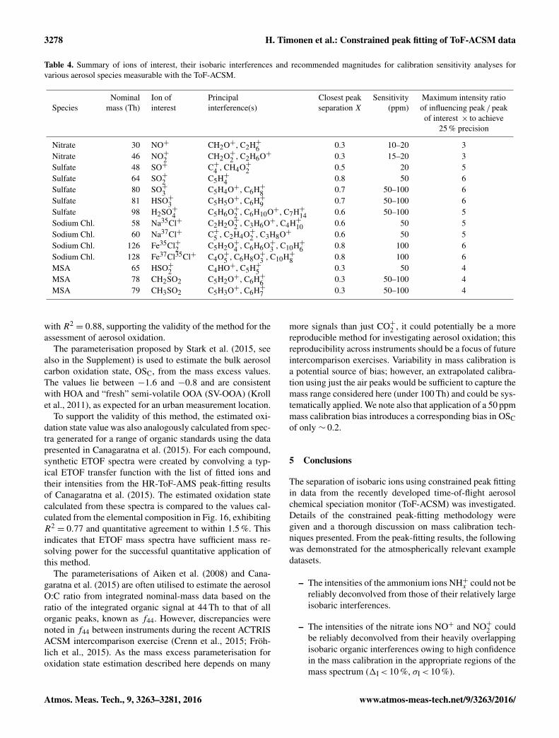
3278 H. Timonen et al.: Constrained peak fitting of ToF-ACSM data
Table 4. Summary of ions of interest, their isobaric interferences and recommended magnitudes for calibration sensitivity analyses forvarious aerosol species measurable with the ToF-ACSM.
Nominal Ion of Principal Closest peak Sensitivity Maximum intensity ratioSpecies mass (Th) interest interference(s) separation X (ppm) of influencing peak / peak
of interest × to achieve25 % precision
Nitrate 30 NO+ CH2O+, C2H+6 0.3 10–20 3Nitrate 46 NO+2 CH2O+2 , C2H6O+ 0.3 15–20 3Sulfate 48 SO+ C+4 , CH4O+2 0.5 20 5Sulfate 64 SO+2 C5H+4 0.8 50 6Sulfate 80 SO+3 C5H4O+, C6H+8 0.7 50–100 6Sulfate 81 HSO+3 C5H5O+, C6H+9 0.7 50–100 6Sulfate 98 H2SO+4 C5H6O+2 , C6H10O+, C7H+14 0.6 50–100 5Sodium Chl. 58 Na35Cl+ C2H2O+2 , C3H6O+, C4H+10 0.6 50 5Sodium Chl. 60 Na37Cl+ C+5 , C2H4O+2 , C3H8O+ 0.6 50 5Sodium Chl. 126 Fe35Cl+2 C5H2O+4 , C6H6O+3 , C10H+6 0.8 100 6Sodium Chl. 128 Fe37Cl35Cl+ C4O+5 , C6H8O+3 , C10H+8 0.8 100 6MSA 65 HSO+2 C4HO+, C5H+5 0.3 50 4MSA 78 CH2SO2 C5H2O+, C6H+6 0.3 50–100 4MSA 79 CH3SO2 C5H3O+, C6H+7 0.3 50–100 4
with R2= 0.88, supporting the validity of the method for the
assessment of aerosol oxidation.The parameterisation proposed by Stark et al. (2015, see
also in the Supplement) is used to estimate the bulk aerosolcarbon oxidation state, OSC, from the mass excess values.The values lie between −1.6 and −0.8 and are consistentwith HOA and “fresh” semi-volatile OOA (SV-OOA) (Krollet al., 2011), as expected for an urban measurement location.
To support the validity of this method, the estimated oxi-dation state value was also analogously calculated from spec-tra generated for a range of organic standards using the datapresented in Canagaratna et al. (2015). For each compound,synthetic ETOF spectra were created by convolving a typ-ical ETOF transfer function with the list of fitted ions andtheir intensities from the HR-ToF-AMS peak-fitting resultsof Canagaratna et al. (2015). The estimated oxidation statecalculated from these spectra is compared to the values cal-culated from the elemental composition in Fig. 16, exhibitingR2= 0.77 and quantitative agreement to within 1.5 %. This
indicates that ETOF mass spectra have sufficient mass re-solving power for the successful quantitative application ofthis method.
The parameterisations of Aiken et al. (2008) and Cana-garatna et al. (2015) are often utilised to estimate the aerosolO:C ratio from integrated nominal-mass data based on theratio of the integrated organic signal at 44 Th to that of allorganic peaks, known as f44. However, discrepancies werenoted in f44 between instruments during the recent ACTRISACSM intercomparison exercise (Crenn et al., 2015; Fröh-lich et al., 2015). As the mass excess parameterisation foroxidation state estimation described here depends on many
more signals than just CO+2 , it could potentially be a morereproducible method for investigating aerosol oxidation; thisreproducibility across instruments should be a focus of futureintercomparison exercises. Variability in mass calibration isa potential source of bias; however, an extrapolated calibra-tion using just the air peaks would be sufficient to capture themass range considered here (under 100 Th) and could be sys-tematically applied. We note also that application of a 50 ppmmass calibration bias introduces a corresponding bias in OSCof only ∼ 0.2.
5 Conclusions
The separation of isobaric ions using constrained peak fittingin data from the recently developed time-of-flight aerosolchemical speciation monitor (ToF-ACSM) was investigated.Details of the constrained peak-fitting methodology weregiven and a thorough discussion on mass calibration tech-niques presented. From the peak-fitting results, the followingwas demonstrated for the atmospherically relevant exampledatasets.
– The intensities of the ammonium ions NH+x could not bereliably deconvolved from those of their relatively largeisobaric interferences.
– The intensities of the nitrate ions NO+ and NO+2 couldbe reliably deconvolved from their heavily overlappingisobaric organic interferences owing to high confidencein the mass calibration in the appropriate regions of themass spectrum (1I< 10 %, σI< 10 %).
Atmos. Meas. Tech., 9, 3263–3281, 2016 www.atmos-meas-tech.net/9/3263/2016/
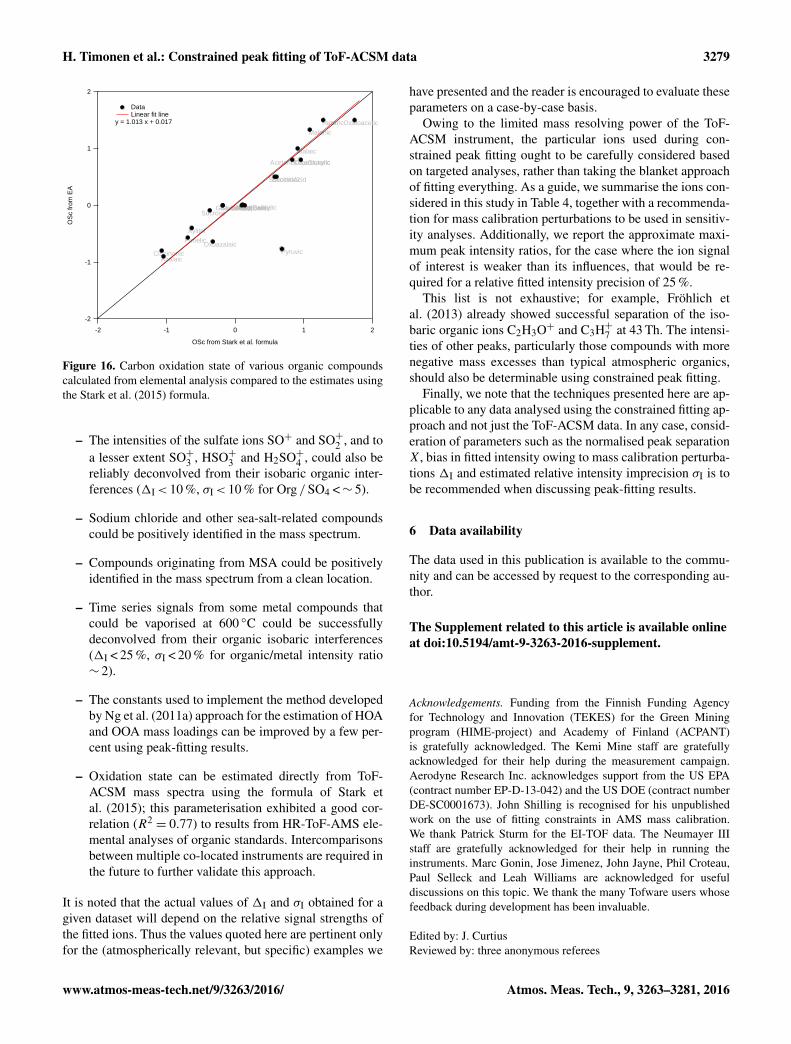
H. Timonen et al.: Constrained peak fitting of ToF-ACSM data 3279
-2
-1
0
1
2
OS
c fr
om E
A
-2 -1 0 1 2
OSc from Stark et al. formula
GlutaricAcid
SuccinicAcid
AcetoneDicarboxylic
AcetylSalicylic
AzalaicCispinonic
DiMethCarbGlutaric2
KetoGlutaric
Ketopimelic
Malaic
Malonic
Oxaloacetic
OxoazalaicPimelic
Pyruvic
Succinic2
Sucrose
Tartaric
Xylitol
Data Linear fit line
y = 1.013 x + 0.017
Figure 16. Carbon oxidation state of various organic compoundscalculated from elemental analysis compared to the estimates usingthe Stark et al. (2015) formula.
– The intensities of the sulfate ions SO+ and SO+2 , and toa lesser extent SO+3 , HSO+3 and H2SO+4 , could also bereliably deconvolved from their isobaric organic inter-ferences (1I< 10 %, σI< 10 % for Org /SO4 <∼ 5).
– Sodium chloride and other sea-salt-related compoundscould be positively identified in the mass spectrum.
– Compounds originating from MSA could be positivelyidentified in the mass spectrum from a clean location.
– Time series signals from some metal compounds thatcould be vaporised at 600 ◦C could be successfullydeconvolved from their organic isobaric interferences(1I < 25 %, σI < 20 % for organic/metal intensity ratio∼ 2).
– The constants used to implement the method developedby Ng et al. (2011a) approach for the estimation of HOAand OOA mass loadings can be improved by a few per-cent using peak-fitting results.
– Oxidation state can be estimated directly from ToF-ACSM mass spectra using the formula of Stark etal. (2015); this parameterisation exhibited a good cor-relation (R2
= 0.77) to results from HR-ToF-AMS ele-mental analyses of organic standards. Intercomparisonsbetween multiple co-located instruments are required inthe future to further validate this approach.
It is noted that the actual values of 1I and σI obtained for agiven dataset will depend on the relative signal strengths ofthe fitted ions. Thus the values quoted here are pertinent onlyfor the (atmospherically relevant, but specific) examples we
have presented and the reader is encouraged to evaluate theseparameters on a case-by-case basis.
Owing to the limited mass resolving power of the ToF-ACSM instrument, the particular ions used during con-strained peak fitting ought to be carefully considered basedon targeted analyses, rather than taking the blanket approachof fitting everything. As a guide, we summarise the ions con-sidered in this study in Table 4, together with a recommenda-tion for mass calibration perturbations to be used in sensitiv-ity analyses. Additionally, we report the approximate maxi-mum peak intensity ratios, for the case where the ion signalof interest is weaker than its influences, that would be re-quired for a relative fitted intensity precision of 25 %.
This list is not exhaustive; for example, Fröhlich etal. (2013) already showed successful separation of the iso-baric organic ions C2H3O+ and C3H+7 at 43 Th. The intensi-ties of other peaks, particularly those compounds with morenegative mass excesses than typical atmospheric organics,should also be determinable using constrained peak fitting.
Finally, we note that the techniques presented here are ap-plicable to any data analysed using the constrained fitting ap-proach and not just the ToF-ACSM data. In any case, consid-eration of parameters such as the normalised peak separationX, bias in fitted intensity owing to mass calibration perturba-tions 1I and estimated relative intensity imprecision σI is tobe recommended when discussing peak-fitting results.
6 Data availability
The data used in this publication is available to the commu-nity and can be accessed by request to the corresponding au-thor.
The Supplement related to this article is available onlineat doi:10.5194/amt-9-3263-2016-supplement.
Acknowledgements. Funding from the Finnish Funding Agencyfor Technology and Innovation (TEKES) for the Green Miningprogram (HIME-project) and Academy of Finland (ACPANT)is gratefully acknowledged. The Kemi Mine staff are gratefullyacknowledged for their help during the measurement campaign.Aerodyne Research Inc. acknowledges support from the US EPA(contract number EP-D-13-042) and the US DOE (contract numberDE-SC0001673). John Shilling is recognised for his unpublishedwork on the use of fitting constraints in AMS mass calibration.We thank Patrick Sturm for the EI-TOF data. The Neumayer IIIstaff are gratefully acknowledged for their help in running theinstruments. Marc Gonin, Jose Jimenez, John Jayne, Phil Croteau,Paul Selleck and Leah Williams are acknowledged for usefuldiscussions on this topic. We thank the many Tofware users whosefeedback during development has been invaluable.
Edited by: J. CurtiusReviewed by: three anonymous referees
www.atmos-meas-tech.net/9/3263/2016/ Atmos. Meas. Tech., 9, 3263–3281, 2016

3280 H. Timonen et al.: Constrained peak fitting of ToF-ACSM data
References
Aiken, A. C., DeCarlo, P. F., and Jimenez, J. L.: ElementalAnalysis of Organic Species with Electron Ionization High-Resolution Mass Spectrometry, Anal. Chem., 79, 8350–8358,doi:10.1021/ac071150w, 2007.
Aiken, A. C., DeCarlo, P. F., Kroll, J. H., Worsnop, D. R., Huff-man, J. A., Docherty, K., Ulbrich, I. M., Mohr, C., Kimmel, J.R., Sueper, D., Sun, Y., Zhang, Q., Trimborn, A., Northway, M.,Ziemann, P. J., Canagaratna, M. R., Onasch, T. B., Alfarra, M.R.,Prevot, A. S. H., Dommen, J., Duplissy, J., Metzger, A., Bal-tensperger, U., and Jiménez, J. L.: O/C and OM/OC Ratios ofPrimary, Secondary, and Ambient Organic Aerosols with a High-Resolution Time-of-Flight Aerosol Mass Spectrometer, Environ.Sci. Technol., 42, 4478–4485, 2008.
Allan, J. D., Coe, H., Bower, K. N., Alfarra, M. R., Delia, A. E.,Jimenez, J. L., Middlebrook, A. M., Drewnick, F., Onasch, T.B., Canagaratna, M. R., Jayne, J. T., and Worsnop, D.R.: Techni-cal Note: Extraction of Chemically Resolved Mass Spectra fromAerodyne Aerosol Mass Spectrometer Data, J. Aerosol Sci., 35,909–922, 2004.
Aurela, M., Saarikoski, S., Niemi, J. V., Canonaco, F., Prevot,A. S. H., Frey, A., Carbone, S., Kousa, A., and Hillamo,R.: Chemical and Source Characterization of Submicron Parti-cles at Residential and Traffic Sites in the Helsinki Metropoli-tan Area, Finland, Aerosol Air Qual. Res, 15, 1213–1226,doi:10.4209/aaqr.2014.11.0279, 2015.
Canagaratna, M. R., Jimenez, J. L., Kroll, J. H., Chen, Q., Kessler,S. H., Massoli, P., Hildebrandt Ruiz, L., Fortner, E., Williams, L.R., Wilson, K. R., Surratt, J. D., Donahue, N. M., Jayne, J. T.,and Worsnop, D. R.: Elemental ratio measurements of organiccompounds using aerosol mass spectrometry: characterization,improved calibration, and implications, Atmos. Chem. Phys., 15,253–272, doi:10.5194/acp-15-253-2015, 2015.
Cappellin, L., Biasioli, F., Granitto, P. M., Schuhfried, E., Souk-oulis, C., Costa, F., Mark, T. D., and Gasperi, F.: On data anal-ysis in PTR-TOF-MS: From raw spectra to data mining, SensorActuat. B-Chem., 155, 183–190, doi:10.1016/j.snb.2010.11.044,2011.
Charlson, R. J., Lovelock, J. E., Andreae, M. O., and Warren, S. G.:Oceanic phytoplankton, atmospheric sulphur, cloud albedo andclimate, Nature, 326, 655–661, 1987.
Corbin, J. C., Othman, A., Allan, J. D., Worsnop, D. R., Haskins, J.D., Sierau, B., Lohmann, U., and Mensah, A. A.: Peak-fitting andintegration imprecision in the Aerodyne aerosol mass spectrom-eter: effects of mass accuracy on location-constrained fits, At-mos. Meas. Tech., 8, 4615–4636, doi:10.5194/amt-8-4615-2015,2015.
Crenn, V., Sciare, J., Croteau, P. L., Verlhac, S., Fröhlich, R., Belis,C. A., Aas, W., Äijälä, M., Alastuey, A., Artiñano, B., Baisnée,D., Bonnaire, N., Bressi, M., Canagaratna, M., Canonaco, F.,Carbone, C., Cavalli, F., Coz, E., Cubison, M. J., Esser-Gietl,J. K., Green, D. C., Gros, V., Heikkinen, L., Herrmann, H., Lun-der, C., Minguillón, M. C., Mocnik, G., O’Dowd, C. D., Ovad-nevaite, J., Petit, J.-E., Petralia, E., Poulain, L., Priestman, M.,Riffault, V., Ripoll, A., Sarda-Estève, R., Slowik, J. G., Setyan,A., Wiedensohler, A., Baltensperger, U., Prévôt, A. S. H., Jayne,J. T., and Favez, O.: ACTRIS ACSM intercomparison – Part1: Reproducibility of concentration and fragment results from13 individual Quadrupole Aerosol Chemical Speciation Moni-
tors (Q-ACSM) and consistency with co-located instruments, At-mos. Meas. Tech., 8, 5063–5087, doi:10.5194/amt-8-5063-2015,2015.
Csavina, J., Field, J., Taylor, M. P., Gao, S., Landázuri, A., Better-ton, E. A., and Sáez, A. E.: A review on the importance of metalsand metalloids in atmospheric dust and aerosol from mining op-erations, Sci. Total Environ., 433, 58–73, 2012.
Cubison, M. J. and Jimenez, J. L.: Statistical precision of the in-tensities retrieved from constrained fitting of overlapping peaksin high-resolution mass spectra, Atmos. Meas. Tech., 8, 2333–2345, doi:10.5194/amt-8-2333-2015, 2015.
DeCarlo, P. F., Kimmel, J. R. Trimborn, A. Northway, M. J. Jayne,J. T. Aiken, A. C., Gonin, M., Fuhrer, K., Horvath, T., Docherty,K., Worsnop, D. R., and Jimenez, J. L.: Field-Deployable, High-Resolution, Time-of-Flight Aerosol Mass Spectrometer, Anal.Chem., 78, 8281–8289, 2006.
Draxler, R. R. and Rolph, G. D.: HYSPLIT (HYbrid Single-ParticleLagrangian Integrated Trajectory) Model, NOAA air ResourcesLaboratory, Silver Spring, MD, available at: http://ready.arl.noaa.gov/HYSPLIT.php, 2013.
Drewnick, F., Hings, S. S., DeCarlo, P., Jayne, J. T., Gonin, M.,Fuhrer, K., Weimer, S., Jimenez, J. L., Demerjian, K. L., Bor-rmann, S., and Worsnop, D. R.: A New Time-of-Flight AerosolMass Spectrometer (TOF-AMS) – Instrument Description andFirst Field Deployment, Aer. Sci. Tech., 39, 637–658, 2005.
Drewnick, F., Diesch, J.-M., Faber, P., and Borrmann, S.: Aerosolmass spectrometry: particle-vaporizer interactions and their con-sequences for the measurements, Atmos. Meas. Tech., 8, 3811–3830, doi:10.5194/amt-8-3811-2015, 2015.
Fröhlich, R., Cubison, M. J., Slowik, J. G., Bukowiecki, N., Prévôt,A. S. H., Baltensperger, U., Schneider, J., Kimmel, J. R., Go-nin, M., Rohner, U., Worsnop, D. R., and Jayne, J. T.: TheToF-ACSM: a portable aerosol chemical speciation monitorwith TOFMS detection, Atmos. Meas. Tech., 6, 3225–3241,doi:10.5194/amt-6-3225-2013, 2013.
Fröhlich, R., Crenn, V., Setyan, A., Belis, C. A., Canonaco, F.,Favez, O., Riffault, V., Slowik, J. G., Aas, W., Aijälä, M.,Alastuey, A., Artiñano, B., Bonnaire, N., Bozzetti, C., Bressi, M.,Carbone, C., Coz, E., Croteau, P. L., Cubison, M. J., Esser-Gietl,J. K., Green, D. C., Gros, V., Heikkinen, L., Herrmann, H., Jayne,J. T., Lunder, C. R., Minguillón, M. C., Mocnik, G., O’Dowd,C. D., Ovadnevaite, J., Petralia, E., Poulain, L., Priestman, M.,Ripoll, A., Sarda-Estève, R., Wiedensohler, A., Baltensperger,U., Sciare, J., and Prévôt, A. S. H.: ACTRIS ACSM intercompar-ison – Part 2: Intercomparison of ME-2 organic source apportion-ment results from 15 individual, co-located aerosol mass spec-trometers, Atmos. Meas. Tech., 8, 2555–2576, doi:10.5194/amt-8-2555-2015, 2015.
Gondwe, M., Krol, M., Gieskes, W., Klaassen, W., and de Baar,H.: The contribution of ocean-leaving DMS to the global atmo-spheric burdens of DMS, MSA, SO2, and NSS SO4, Global Bio-geochem. Cy., 17, 1056, doi:10.1029/2002GB001937, 2003.
IPCC: Climate Change 2013: The Physical Science Basis, Contri-bution of Working Group I to the Fifth Assessment Report of theIntergovernmental Panel on Climate Change, edited by: Stocker,T. F., Qin, D., Plattner, G.-K., Tignor, M., Allen, S. K., Boschung,J., Nauels, A., Xia, Y., Bex, V., and Midgley P. M., CambridgeUniversity Press, Cambridge, United Kingdom and New York,NY, USA, 1535 pp., 2013.
Atmos. Meas. Tech., 9, 3263–3281, 2016 www.atmos-meas-tech.net/9/3263/2016/
H. Timonen et al.: Constrained peak fitting of ToF-ACSM data 3281
Jayne, J. T., Leard, D. C., Zhang, X., Davidovits, P., Smith, K. A.,Kolb, C. E., and Worsnop, D. R.: Development of aerosol massSpectrometer for Size and Composition Analysis of SubmicronParticle, Aerosol Sci. Tech, 33, 49–70, 2000.
Jimenez, J. L., Jayne, J. T., Shi, Q., Kolb, C. E., Worsnop, D. R.,Yourshaw, I., Seinfeld, J. H., Flagan, R. C., Zhang, X., Smith,K. A., Morris, J., and Davidovits, P.: Ambient Aerosol Samplingwith an Aerosol Mass Spectrometer, J. Geophys. Res.-Atmos.,108, 8425, doi:10.1029/2001JD001213, 2003.
Junninen, H., Ehn, M., Petäjä, T., Luosujärvi, L., Kotiaho, T., Kos-tiainen, R., Rohner, U., Gonin, M., Fuhrer, K., Kulmala, M., andWorsnop, D. R.: A high-resolution mass spectrometer to mea-sure atmospheric ion composition, Atmos. Meas. Tech., 3, 1039–1053, doi:10.5194/amt-3-1039-2010, 2010.
Järvi, L., Hannuniemi, H., Hussein, T., Junninen, H., Aalto, P. P.,Hillamo, R., Mäkela, T., Keronen, P., Siivola, E., Vesala, T., andKulmala, M.: The urban measurement station SMEAR III: Con-tinuous monitoring of air pollution and surface-atmosphere inter-actions in Helsinki, Finland, Boreal Environ. Res., 14, 86–109,2009.
Kendrick, E.: A mass scale based on CH2 = 14.0000 for high res-olution mass spectrometry of organic compounds, Anal. Chem,35, 2146–2154, 1963.
Kimmel, J. R., Farmer, D. K., Cubison, M. J., Sueper, D., Tanner, C.,Nemitz, E., Worsnop, D. R., Gonin, M., and Jimenez J. L.: Real-time Aerosol Mass Spectrometry with Millisecond Resolution,Int. J. Mass Spec, 303, 15–26, doi:10.1016/j.ijms.2010.12.004,2011.
Kroll, J. H., Donahue, N. M., Jimenez, J. L., Kessler, S. H., Cana-garatna, M. R., Wilson, K. R., Altieri, K. E., Mazzoleni, L. R.,Wozniak, A. S., Bluhm, H., Mysak, E. R., Smith, J. D., Kolb, C.E., and Worsnop D. R.: Carbon Oxidation State as a Metric forDescribing the Chemistry of Atmospheric Organic Aerosol, Nat.Chem., 3, 133–139, doi:10.1038/NCHEM.948, 2011.
Korhonen, H., Carslaw, K. S., Spracklen, D. V., Mann, G.W., and Woodhouse, M. T.: Influence of oceanic dimethylsulfide emissions on cloud condensation nuclei concentra-tions and seasonality over the remote Southern Hemisphereoceans: A global model study, J. Geophys. Res., 113, D15204,doi:10.1029/2007jd009718, 2008.
Lawson, C. L. and Hanson, R. J.: Solving Least Squares Problems,SIAM, 1995.
Meija, J. and Caruso, J. A.: Deconvolution of isobaric interferencesin mass spectra, J. Am. Soc. Mass Spectrom., 15, 654–658, 2004.
Müller, M., Mikoviny, T., Jud, W., D’Anna, B., and Wisthaler, A.:A new software tool for the analysis of high resolution PTR-TOFmass spectra, Chemometr. Intell. Lab., 127, 158–165, 2013.
Ng, N. L., Canagaratna, M. R., Jimenez, J. L., Zhang, Q., Ulbrich,I. M., and Worsnop, D. R.: Real-time methods for estimating or-ganic component mass concentrations from aerosol mass spec-trometer data, Environ. Sci. Technol., 45, 910–916, 2011a.
Ng, N. L., Herndon, S. C., Trimborn, A., Canagaratna, M. R.,Croteau, P. L., Onasch, T. B., Sueper, D., Worsnop, D. R., Zhang,Q., Sun, Y. L., and Jayne, J. T.: An Aerosol Chemical SpeciationMonitor (ACSM) for Routine Monitoring of the Compositionand Mass Concentrations of Ambient Aerosol. Aer. Sci. Tech.,45, 780–794, doi:10.1080/02786826.2011.560211, 2011b.
Ortega, A. M., Day, D. A., Cubison, M. J., Brune, W. H., Bon,D., de Gouw, J. A., and Jimenez, J. L.: Secondary organicaerosol formation and primary organic aerosol oxidation frombiomass burning smoke in a flow reactor during FLAME-3, At-mos. Chem. Phys., 13, 13799–13851, 2013
Ovadnevaite, J., Ceburnis, D., Canagaratna, M., Berresheim, H.,Bialek, J., Martucci, G., Worsnop, D. R., and O’Dowd, C.: Onthe effect of wind speed on submicron sea salt mass concentra-tions and source fluxes, J. Geophys. Res.-Atmos., 117, D16201,10.1029/2011jd017379, 2012.
Phinney, L., Leaitch, W., Lohmann, U., Boudries, H., Worsnop, D.R., Jayne, J. T., Toom-Sauntry, D., Wadleigh, M., Sharma, S., andShantz, N.: Characterization of the aerosol over the sub-arcticnorth east Pacific Ocean, Deep-Sea Res. Pt. II, 53, 2410–2433,doi:10.1016/j.dsr2.2006.05.044, 2006.
Pope, C. A. and Dockery, D. W.: Health Effects of Fine ParticulateAir Pollution: Lines that Connect, J. Air Waste Manage. Assoc.,56, 709–742, 2006.
Salcedo, D., Laskin, A., Shutthanandan, V., and Jimenez, J. L.: Fea-sibility of the Detection of Trace Elements in Particulate MatterUsing Online High-Resolution Aerosol Mass Spectrometry, Aer.Sci. Tech., 46, 1187–1200, doi:10.1080/02786826.2012.701354,2012.
Schmale, J., Schneider, J., Nemitz, E., Tang, Y. S., Dragosits, U.,Blackall, T. D., Trathan, P. N., Phillips, G. J., Sutton, M., andBraban, C. F.: Sub-Antarctic marine aerosol: dominant contri-butions from biogenic sources, Atmos. Chem. Phys., 13, 8669–8694, doi:10.5194/acp-13-8669-2013, 2013.
Stark, H., Yatavelli, R. N. L., Thompson, S. L., Kimmel, J. R., Cu-bison, M. J., Chhabra, P. J., Canagaratna, M. R., Jayne, J. T.,Worsnop, D. R., and Jimenez, J. L.: Methods to extract molecu-lar and bulk chemical information from series of complex massspectra with limited mass resolution, Int. J. Mass Spec., 289, 26–38, doi:10.1016/j.ijms.2015.08.011, 2015.
Sueper, D.: ToF-AMS High Resolution Analysis Software– Pika, available at: http://cires.colorado.edu/jimenez-group/ToFAMSResources/ToFSoftware/PikaInfo, 2008.
Weller, R., Minikin, A., Wagenbach, D., and Dreiling, V.: Char-acterization of the inter-annual, seasonal, and diurnal variationsof condensation particle concentrations at Neumayer, Antarc-tica, Atmos. Chem. Phys., 11, 13243–13257, doi:10.5194/acp-11-13243-2011, 2011.
Weller, R., Schmidt, K., Teinilä, K., and Hillamo, R.: Naturalnew particle formation at the coastal Antarctic site Neumayer,Atmos. Chem. Phys., 15, 11399–11410, doi:10.5194/acp-15-11399-2015, 2015.
Yin, F., Grosjean, D., Flagan, R. C., and Seinfeld, J. H.: Photoox-idation of dimethyl sulfide and dimethyl disulfide: Mechanismsevaluation, J. Atmos. Chem, 11, 365–399, 1990.
Zahradník, P. and Vlcek M.: Fast Analytical Design Algorithms forFIR Notch Filters, IEEE T. Circuits Syst., 51, 608–623, 2004.
www.atmos-meas-tech.net/9/3263/2016/ Atmos. Meas. Tech., 9, 3263–3281, 2016