ry Systems 88 (2007) 197–203www.elsevier.com/locate/chemolab

Chemometrics and Intelligent Laborato

Application of the replacement method as novel variable selection inQSPR. 2. Soil sorption coefficients

Pablo R. Duchowicz a,⁎, Maykel Pérez González b, Aliuska Morales Helguera b,c,d,Maria Natália Dias Soeiro Cordeiro d, Eduardo A. Castro a

a Instituto de Investigaciones Fisicoquímicas Teóricas y Aplicadas (INIFTA), Facultad de Ciencias Exactas, Diag. 113 y 64,Suc. 4, C.C. 16, (1900) La Plata, Argentina

b Chemical Bioactive Center, Central University of Las Villas, Santa Clara, 54830 Villa Clara, Cubac Department of Chemistry, Faculty of Chemistry and Pharmacy, Central University of Las Villas, Santa Clara, Villa Clara, Cuba

d REQUIMTE, Chemistry Department, Faculty of Sciences, University of Porto, 4169-007 Porto Portugal

Received 12 December 2006; received in revised form 1 May 2007; accepted 3 May 2007Available online 13 May 2007

Abstract

We predict the soil sorption coefficients of 163 non-ionic organic pesticides performing a QSPR treatment. A pool containing 1247 theoreticaldescriptors is explored simultaneously encoding different aspects of the topological, geometrical, and electronic molecular structure. Theapplication of Forward Stepwise Regression, Genetic Algorithms and the Replacement Method leads to an optimal six-parameter equationcharacterized with R=0.949 and that also exhibits good cross-validated predictive ability, Rl-25%-o=0.916. This model compares fairly well with apreviously reported QSPR on the same data set with R=0.904.© 2007 Elsevier B.V. All rights reserved.

Keywords: QSPR theory; Organic pesticide; KOC; Genetic algorithms; Replacement method

1. Introduction

The reliable estimation of soil sorption coefficients (KOC) fororganic pesticides plays a fundamental role in Agriculture,especially for describing the pollution impact of the pesticidesand their tendency for biodegradation. This partition coefficientrepresents ameasure of the retaining of a chemical by the organicmatter of soils and sediments through a wide variety of possibleintermolecular interactions [1,2]. Nowadays, less than 300chemicals have measured their KOC values, and little informa-tion is available on the sorption behavior of their metabolites [3].Clearly, the prediction of the KOC parameter for a wide numberof chemical structures is very convenient for application in riskassessment.

A generally accepted remedy to surmount the lack ofavailability of experimental data in contemporary Chemistry is

⁎ Corresponding author. Fax: +54 221 425 4642.E-mail addresses: prduchowicz@yahoo.com.ar, duchow@inifta.unlp.edu.ar

(P.R. Duchowicz).

0169-7439/$ - see front matter © 2007 Elsevier B.V. All rights reserved.doi:10.1016/j.chemolab.2007.05.001

the application of a Quantitative Structure-Property Relationships(QSPR) analysis [4], in the present case to obtain adequatepredictions for soil sorption coefficients. The ultimate role of thedifferent formulations of the QSPR theory is to suggest mathe-matical models for estimating relevant endpoints of interest,especially when these cannot be experimentally determined forsome reason. These studies simply rely on the assumption thatthe structure of a compound determinates the physicochemicalproperties it manifests. The molecular structure is thereforetranslated into the so-called molecular descriptors throughmathematical formulae obtained from several theories, such asChemical Graph Theory, Information Theory, QuantumMechan-ics, etc. [5,6] There exist more than a thousand of theoreticaldescriptors available in the literature, and one usually faces theproblem of selecting those which are the most representatives forthe property under consideration.

More than 200 models have been reviewed in the literaturefor the estimation of the KOC parameter for non-ionic organicchemicals [7], among these nearly 80 relate to pesticides. However,these models are mainly class-specific and are often obtained with

Table 1Experimental and predicted values Eq. (6) of log KOC and comparison withvalues reported in a previous study

ID Name CAS Exp. Pred. Ref. [8]

Acetanilides1 Acetochlor 34256-82-1 2.32 2.63 2.422 Alachlor 15972-60-8 2.28 2.43 2.533 Butachlor 23184-66-9 2.86 3.30 3.064 Metalaxyl 57837-19-1 1.57 1.71 2.055 Metolachlor 51218-45-2 2.46 2.40 2.436 Propachlor 1918-16-7 2.42 2.05 2.18

Carbamates7 Aldicarb 116-03-3 1.50 1.93 1.978 Aldicarb sulfone 1646-88-4 0.42 1.13 1.739 Benomyl 17804-35-2 2.71 2.26 1.9210 Butylate 2008-41-5 2.11 2.00 2.1311 Carbaryl 63-25-2 2.40 2.39 2.1312 Carbendazim (MBC) 10605-21-7 2.35 2.02 1.7513 Carbofuran 1563-66-2 1.75 2.12 2.0114 Chlorpropham 101-21-3 2.53 2.29 2.0515 Cycloate 1134-23-2 2.54 2.07 2.0616 Diallate (cis) 2303-16-4 3.28 3.14 2.6617 Diallate (trans) 2303-16-4 3.28 3.14 2.6518 EPTC 759-94-4 2.38 1.93 1.9819 Methiocarb 2032-65-7 2.32 2.52 2.2220 Methomyl 16752-77-5 1.30 1.40 1.6221 Molinate 2212-67-1 1.92 1.77 1.8622 Oxamyl 23135-22-0 1.00 1.39 1.6823 Pebulate 1114-71-2 2.80 2.25 2.1024 Methyl-N-phenylcarbamate 2603-10-3 1.73 1.64 1.6425 Ethyl-N-phenylcarbamate 101-99-5 1.82 1.73 1.7326 Propyl-N-phenylcarbamate 5532-90-1 2.06 1.94 1.8727 Butyl-N-phenylcarbamate 1538-74-5 2.26 2.22 2.1028 Pentyl-N-phenylcarbamate 63075-06-9 2.61 2.72 2.3829 Methyl-N-(3-chlorophenyl)

carbamate2150-88-1 2.15 2.05 1.86

30 Methyl-N-(3,4-dichlorophenyl)carbamate

1918-18-9 2.74 2.77 2.32

31 Propham 122-42-9 1.83 1.83 1.8532 Propoxur 114-26-1 1.67 1.94 1.8833 Thiobencarb 28249-77-6 3.27 3.23 2.7534 Triallate 2303-17-5 3.35 3.52 3.1235 Vernolate 1929-77-7 2.33 2.20 2.11

Dinitroanilines36 Benfluralin 1861-40-1 3.99 3.96 3.8437 Butralin 33629-47-9 3.98 3.27 3.3838 Dinitramine 29091-05-2 3.63 3.26 3.4239 Fluchloralin 33245-39-5 3.55 3.79 4.0240 Nitralin 4726-14-1 2.92 2.86 3.2841 Oryzalin 19044-88-3 3.40 2.98 3.1842 Profluralin 26399-36-0 4.01 3.74 3.8743 Trifluralin 1582-09-8 3.93 3.83 3.86

Organochlorides44 Aldrin 309-00-2 4.69 4.33 4.6845 Chlordane 12709-03-6 5.15 4.71 5.0346 p,p-DDT 50-29-3 5.31 5.15 5.1747 p,p-DDE 72-55-9 4.82 5.33 4.8548 Dieldrin 60-57-1 4.55 4.23 4.7149 Endosulfan 115-29-7 4.13 4.03 3.9050 Lindane 58-89-9 3.00 3.59 4.5751 Methoxychlor 72-43-5 4.90 4.70 4.68

Table 1 (continued )

ID Name CAS Exp. Pred. Ref. [8]

Organophosphates52 Azinphos methyl 86-50-0 2.28 2.64 2.0453 Carbophenothion 786-19-6 4.66 4.79 4.0854 Chlorfenvinphos (cis) 18708-87-7 2.47 2.78 3.0455 Chlorfenvinphos (trans) 18708-86-6 2.47 2.81 3.1156 Chlorpyrifos 2921-88-2 3.70 3.36 3.7657 Chlorpyrifos (methyl) 5598-13-0 3.52 3.20 3.4958 Crotoxyphos (trans) 7700-17-6 2.00 2.27 2.5959 Diazinon 333-41-5 2.75 2.63 3.0560 Dicrotophos (cis) 141-66-2 1.66 0.87 1.6761 Dimethoate 60-51-5 1.20 1.94 1.8562 Disulfoton 298-04-4 3.22 3.24 3.4063 Ethion 563-12-2 4.06 3.84 3.9564 Ethoprophos 13194-48-4 1.80 2.21 2.3065 Fenamiphos 22224-92-6 2.51 2.50 2.3066 Fenitrothion 122-14-5 2.63 2.69 2.7667 Fensulfothion 115-90-2 2.52 2.53 2.6468 Fonofos 944-22-9 3.44 3.01 3.0469 Isazophos 42509-80-8 2.01 2.43 2.9170 Malathion 121-75-5 3.07 2.15 2.2971 Mevinphos (cis) 7786-34-7 0.85 0.75 1.5672 Mevinphos (trans) 338-45-4 0.85 0.54 1.6773 Parathion ethyl 56-38-2 3.20 2.97 3.1474 Parathion methyl 298-00-0 3.00 2.67 2.8475 Phorate 298-02-2 2.70 3.05 3.1276 Phosalone 2310-17-0 3.71 3.80 2.8977 Profenofos 41198-08-7 3.03 3.43 3.1978 Terbufos 13071-79-9 2.82 3.19 3.3079 Trichlorfon 52-68-6 1.90 1.94 2.25

Phenylureas80 Phenylurea 64-10-8 1.50 1.44 1.6081 2-Chlorophenylurea 114-38-5 1.61 1.88 1.8582 2-Fluorophenylurea 656-31-5 1.32 1.48 1.3683 3-Chlorophenylurea 1967-27-7 2.01 1.95 1.8584 3-Fluorophenylurea 770-19-4 1.77 1.61 1.4185 3-Bromophenylurea 2989-98-2 2.12 2.27 2.2286 3-Methylphenylurea 63-99-0 1.56 1.56 1.6687 3-Trifluoromethylphenylurea 13114-87-9 1.98 1.94 2.2288 4-Fluorophenylurea 659-30-3 1.52 1.61 1.6889 4-Bromophenylurea 1967-25-5 2.06 2.11 2.4290 4-Phenoxyphenylurea 78508-44-8 2.56 2.69 2.8491 3,4-Dichlorophenylurea 2327-02-8 2.53 2.52 2.3292 3-Chloro-4-

methoxyphenylurea25277-05-8 2.00 1.91 1.96

93 3-Methyl-4-fluorophenylurea 78508-45-9 1.75 1.68 1.6394 3-Methyl-4-bromophenylurea 78508-46-0 2.37 2.18 2.4695 N-Phenyl-N′-cyclopropylurea 13140-86-8 1.74 1.58 1.8496 N-Phenyl-N′-cyclopentylurea 13140-89-1 1.93 2.05 2.1897 N-Phenyl-N′-cyclohexylurea 86759-64-0 2.07 2.22 2.3898 N-Phenyl-N′-cycloheptylurea 19095-79-5 2.37 2.28 2.5599 Siduron 1982-49-6 2.31 2.30 2.25100 N-Phenyl-N-methylurea 4559-87-9 1.29 1.40 1.62101 N-(3-Chlorophenyl)-

N′-methylurea20940-42-5 1.93 1.86 1.84

102 N-(3,4-Dichlorophenyl)-N′-methylurea

3567-62-2 2.46 2.34 2.32

103 N-(3-Chloro-4-methylphenyl)-N′-methylurea

22175-22-0 2.10 1.95 2.07

104 N-(3-Chloro-4-methoxyphenyl)-N′-methylurea

20782-57-4 1.84 2.14 2.04

198 P.R. Duchowicz et al. / Chemometrics and Intelligent Laboratory Systems 88 (2007) 197–203

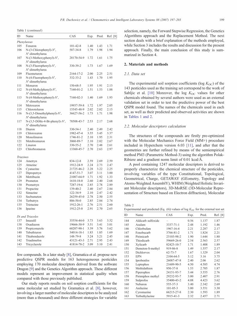
Table 2Experimental and predicted (Eq. (6)) values of log KOC for the external test set

ID Name CAS Exp. Pred. Ref. [8]

144 Aldicarb sulfoxide – 0.56 1.137 1.87145 Asulam 3337-71-1 2.48 1.192 1.46146 Chlorbufam 1967-16-4 2.21 2.287 2.17147 Fenobucarb 3766-81-2 1.71 1.824 2.21148 Pirimicarb 23103-98-2 1.90 1.644 1.80149 Thiodicarb 59669-26-0 2.54 2.563 2.57150 Xylicarb 02425-10-7 1.71 1.408 1.89151 Demeton-S-methyl 919-86-8 1.49 1.557 2.17152 Dichlorvos 62-73-7 1.67 1.329 2.04153 EPN 2104-64-5 3.12 3.16 3.75154 Iprobenfos 26087-47-8 2.40 2.06 2.62155 Leptophos 21609-90-5 4.50 4.585 4.74156 Methidathion 950-37-8 1.53 2.705 1.87157 Piperophos 24151-93-7 3.44 3.555 2.76158 Pirimiphos methyl 29232-93-7 3.00 2.407 2.91159 Sulprofos 35400-43-2 4.08 4.423 3.62160 Neburon 555-37-3 3.40 2.342 2.69161 Anilazine 101-05-3 3.00 3.551 3.30162 Cyromazine 66215-27-8 2.30 1.593 1.89163 Terbuthylazine 5915-41-3 2.32 2.457 2.71

Table 1 (continued )

ID Name CAS Exp. Pred. Ref. [8]

Phenylureas105 Fenuron 101-42-8 1.40 1.43 1.71106 N-(3-Chlorophenyl)-N′,

N′-dimethylurea587-34-8 1.79 1.98 1.94

107 N-(3-Methoxyphenyl)-N′,N′-dimethylurea

28170-54-9 1.72 1.61 1.75

108 N-(3-Fluorophenyl)-N′,N′-dimethylurea

330-39-2 1.73 1.67 1.69

109 Fluometuron 2164-17-2 2.00 2.25 2.51110 N-(4-Fluorophenyl)-N′,

N′-dimethylurea332-33-2 1.43 1.70 1.95

111 Monuron 150-68-5 1.95 1.91 2.13112 N-(4-Methylphenyl)-N′,

N′-dimethylurea7160-01-2 1.51 1.53 1.88

113 N-(4-Methoxyphenyl)-N′,N′-dimethylurea

7160-02-3 1.40 1.69 1.93

114 Metoxuron 19937-59-8 1.72 1.97 2.05115 Chlorotoluron 15545-48-9 2.02 2.02 2.15116 N-(3,5-Dimethylphenyl)-N′,

N′-dimethylurea36627-56-2 1.73 1.71 1.98

117 N-(3,5-DiMe-4-Br-phenyl)-N′,N′-dimethylurea

78508-43-7 2.53 2.17 2.68

118 Diuron 330-54-1 2.40 2.49 2.42119 Chloroxuron 1982-47-4 3.55 3.45 3.37120 Monolinuron 1746-81-2 2.10 1.95 2.31121 Metobromuron 3060-89-7 2.10 2.02 2.67122 Linuron 330-55-2 2.70 2.48 2.61123 Chlorbromuron 13360-45-7 2.70 2.63 2.97

Triazines124 Ametryn 834-12-8 2.59 2.69 2.59125 Atrazine 1912-24-9 2.24 2.73 2.47126 Cyanazine 21725-46-2 2.28 3.22 2.25127 Dipropetryn 4147-51-7 3.07 3.11 3.00128 Metribuzin 21087-64-9 1.71 1.92 1.33129 Prometon 1610-18-0 2.60 2.40 2.68130 Prometryn 7287-19-6 2.85 2.78 2.89131 Propazine 139-40-2 2.40 2.67 2.84132 Simazine 122-34-9 2.10 2.47 2.42133 Secbumeton 26259-45-0 2.78 2.50 2.55134 Terbutryn 886-50-0 2.85 2.84 2.74135 Trietazine 1912-26-1 2.76 2.51 2.60136 Ipazine 1912-25-0 2.91 2.70 2.65

Di and Triazoles137 Imazalil 35554-44-0 3.73 3.63 3.52138 Oxadiazon 19666-30-9 3.51 3.41 3.01139 Propiconazole 60207-90-1 3.39 3.76 3.62140 Tebuthiuron 34014-18-1 1.83 1.85 1.69141 Thiabendazole 148-79-8 3.24 3.21 2.45142 Triadimefon 43121-43-3 2.71 2.95 2.43143 Tricyclazole 41814-78-2 3.09 3.10 2.41

199P.R. Duchowicz et al. / Chemometrics and Intelligent Laboratory Systems 88 (2007) 197–203

few compounds. In a later study [8], Gramatica et al. propose newpredictive QSPR models for 163 heterogeneous pesticidesemploying 170 molecular descriptors derived from the softwareDragon [9] and the Genetics Algorithm approach. These differentmodels represent an improvement in statistical quality whencompared with those previously published.

Our study reports results on soil sorption coefficients for thesame molecular set studied by Gramatica et al. [8], however,involving a larger number of molecular descriptors to be analyzed(more than a thousand) and three different strategies for variable

selection, namely, the Forward Stepwise Regression, the GeneticsAlgorithms approach and the Replacement Method. The nextsection deals with a brief explanation of the methods employed,while Section 3 includes the results and discussion for the presentapproach. Finally, the main conclusion of this study is sum-marized in Section 4.

2. Materials and methods

2.1. Data set

The experimental soil sorption coefficients (log KOC) of the143 pesticides used as the training set correspond to the work ofSabljic et al. [10] Moreover, the log KOC values for otherchemicals obtained by several authors were used as an externalvalidation set in order to test the predictive power of the bestQSPR model found. The names of the chemicals used in eachset, as well as their predicted and observed activities are shownin Tables 1 and 2.

2.2. Molecular descriptors calculation

The structures of the compounds are firstly pre-optimizedwith the Molecular Mechanics Force Field (MM+) procedureincluded in Hyperchem version 6.03 [11], and after that thegeometries are further refined by means of the semiempiricalmethod PM3 (Parametric Method-3) using the algorithm Polak-Ribiere and a gradient norm limit of 0.01 kcal/Å.

A pool containing 1247 molecular descriptors is derived toproperly characterize the chemical structure of the pesticides,involving variables of the type Constitutional, Topological,Geometrical, Charge, GETAWAY (GEometry, Topology andAtoms-Weighted AssemblY),WHIM (Weighted Holistic Invari-ant Molecular descriptors), 3D-MoRSE (3D-Molecular Repre-sentation of Structure based on Electron diffraction), Molecular

200 P.R. Duchowicz et al. / Chemometrics and Intelligent Laboratory Systems 88 (2007) 197–203

Walk Counts, BCUT descriptors, 2D-Autocorrelations, Aroma-ticity Indices, Randić molecular profiles, Radial DistributionFunctions, Functional Groups and Atom-Centred Fragments.These variables are calculated by means of the software Dragonversion 5.4 [9]. We excluded the empirical and property-baseddescriptors in order to avoid the uncertainty of experimentallyderived input-variables. Four quantum-chemical descriptorswere also added to the pool (not provided by Dragon): moleculardipole moments, total energies, and homo-lumo energies.

We proceed now to describe briefly the three different tech-niques employed for searching the best descriptors via linearregression formulae.

2.3. Variable selection strategy

2.3.1. Forward stepwise regressionThe Forward Stepwise Regression procedure [12] (FSR) is an

interesting approach both from the didactical point of view andfor the simplicity of the algorithm that involves. It consists on astep by step addition of the best molecular descriptors to themodel that lead to the smallest value of the standard deviation(S), until there is no-other variable outside the equation thatsatisfies the selection criterion. The definition of S employed inpresent analysis is as follows:

S ¼ 1N � d � 1

XNi¼1

res2i

!ð1Þ

with d being the number of descriptors of the model, N is thenumber of molecules of the training set, and resi stands for theresidual of molecule i (difference between the experimental andpredicted property for i). The FSR technique requires much lesslinear regressions than a Full Search of optimal variables (FS).

2.3.2. The genetic algorithm approachThe Genetic Algorithm (GA) [13–15] introduced by John

Holland has been considered superior to other method of vari-able selection techniques. It is a search paradigm inspired bynatural evolution where the variables are represented as geneson a chromosome (model). It is similar to simplex optimizationand evolves from a group of random initial models (population)with fitness scores and searches for chromosomes with betterfitness functions (response function scores) through naturalselection and the genetic operators, mutation and recombina-tion. The natural selection guarantees the propagation of chro-mosomes with better fitness in future populations. The GAcombines genes from two parent chromosomes using the ge-netic recombination operator to form two new chromosomes(children) that have a high probability of having better fitnessthan their parents, and also explores new response surface (localoptima) through mutation. The GAs offering a combination ofhill-climbing ability (natural selection) and a stochastic method(recombination and mutation) are very flexible because theyoptimize on a representation of variables, not the variablesthemselves. In addition, the GAs provide efficient optimizationas they use implicit parallelism to process information quickly

and require fewer response function evaluations than otherautomated numerical optimization algorithms.

2.3.3. The replacement methodBecause the selection of a representative subset of optimal

descriptors from a pool containing thousands of them is verycomputational demanding,we proposed theReplacementMethod(RM) [16–18] as an algorithm that yields results comparable to acombinatorial search (full search) of optimal variables with muchless linear regressions. Also, RM produces similar results to themore elaborated GA procedure. The main idea behind the RM isthat one can approach the minimum of S by judiciously takinginto account the relative errors of the coefficients of the least-squares model given by a set of d descriptors d={X1, X2,…, Xd}.In other words, we should find the global minimum of S(d) in asubspace ofD! / [d!(D−d)!] points d, whereD represents the totalnumber of available descriptors.

2.4. Models comparison and validation

The quality of the final optimized equations obtained via thethree approaches FSR, GA and RM was compared by means ofthe classical statistical parameters correlation coefficient (R), S,F (Fisher ratio) and two further criteria: the Akaike criterion andthe Kubinyi function. Akaike's information criterion (AIC)[19,20] formulated in 1973 takes into account the statisticalgoodness of fit and the number of parameters that have to beestimated to achieve that degree of fit. This criterion is calculatedusing the following equation:

AIC ¼XNi¼1

res2i

!� N þ dð ÞN � dð Þ2 ð2Þ

When comparing models, the model that produces theminimum AIC value should be considered potentially the mostuseful. The Kubinyi function (FIT) [13,14] closely relates to Fand was proved to be a useful parameter assessing the quality ofthe models:

FIT ¼ R2 � N � d � 1ð ÞN þ d2ð Þ � 1� R2ð Þ ð3Þ

The main disadvantage of the F value is its sensitivity tochanges in d, if d is small, and its lower sensitivity if d is large.The FIT criterion has a low sensitivity toward changes in dvalues, as long as they are small numbers, and a substantiallyincreasing sensitivity for large d values. Finally, the best modelwill present the highest value of this function.

In order to elucidate the predictive power of the finalrelationships found during the calibration step, it is mandatoryto perform the validation of the models. The theoreticalvalidation practiced on our equations is based on the leave-one-out (loo) and leave-more-out cross validation procedures (l-n%-o) [21], with n% representing the percentage of moleculesremoved from the training set. The number of cases analyzedfor random exclusion of n% of the molecules in l-n%-o is90,000. Finally, the QSPR equations found are further validated

Table 3Description for the molecular descriptors appearing in the QSPR

Symbol Classification Description

ATS1v 2D-Autocorrelations[26,27]

Broto–Moreau autocorrelation of atopological structure — lag 1 /weightedby atomic Van der Waals volumes

HATS0e GETAWAY [30] Leverage-weighted autocorrelationof lag 0 /weighted by atomicSanderson electronegativities

G(Cl…Cl) Geometrical [31] Sum of geometrical distances betweenCl…Cl

GATS1e 2D-Autocorrelations Geary autocorrelation — lag1 /weighted by atomicSanderson electronegativities

O-058 Atom-centredfragments [32]

Number of O=fragments

nP Constitutional [31] Number of phosphorous atomsVm WHIM [28,29] V total size index /weighted by

atomic massesATS2p 2D-Autocorrelations Broto-Moreau autocorrelation of a

topological structure — lag2 /weighted by atomic polarizabilities

nCONN Functional Groups [31] Number of urea derivativesDs WHIM D total accessibility index/weighted

by atomic electrotopological statesZM2 Topological [5,31] Second Zagreb index M2PHI Topological Kier flexibility indexRgyr Geometrical Radius of gyration (mass weighted)N-076 Atom-centred fragments Ar–NO2/R–N(–R)–O/RO–NO2

a

a Ar: aromatic group, R: aliphatic group, – represents aromatic single bonds asthe C–N bond in pyrrole.

201P.R. Duchowicz et al. / Chemometrics and Intelligent Laboratory Systems 88 (2007) 197–203

by means of an external prediction set composed of pesticidesnot used to develop the prediction function.

2.5. Orthogonalization procedure

We employ the orthogonalization procedure introducedseveral years ago by Randić [22–24] as a way of improvingthe statistical interpretation of the model built by interrelatedindices. From our point of view, the co-linearity of the mole-cular descriptors should be as low as possible, because theinterrelatedness among the different descriptors can lead tohighly unstable regression coefficients, which makes itimpossible to know the relative importance of an index andunderestimates the utility of the regression coefficients of themodel. The crucial step of the orthogonalization process is thechoice of an appropriate order of orthogonalization, which inpresent analysis is the order that maximises the correlationbetween each descriptor and the observed partition coefficients.

3. Results and discussion

We began the analysis by employing the GA technique to search forthe optimal linear model containing the best molecular descriptors. Allthe QSPR reported here were searched in such a way to fulfill thefollowing three criteria: (a) the best l-n%-o cross-validation parametersRl-n%-o and Sl-n%-o, with n%=25% (35 randomly removed compoundsfrom the training set); (b) the least number of descriptors in the model;(c) the least number of outlier compounds (compounds with a residualexceeding the value 3S). These conditions lead to a linear equationcontaining six descriptors of 1D, 2D and 3D dimensionality:

log Koc ¼ �4:031 F0:4ð Þ þ 0:005 F0:002ð Þ � ZM2þ 0:154 F0:03ð Þ � PHI þ 7:977 F0:6ð Þ � ATS1vþ 0:213 F0:04ð Þ � RGyr � 0:503 F0:05ð Þ � O�058þ 0:243 F0:06ð Þ � N � 076 ð4Þ

N=143 R=0.944 S=0.305 F=186.400 Rloo=0.940 Sloo=0.317Rl-25%-o=0.914 Sl-25%-o=0.370 AIC=0.103 FIT=6.191A brief description for each variable appearing in all the proposed

models is also presented in Table 3. The application of the FSRtechnique does not improve the quality of this statistics, resulting in thefollowing model:

log Koc ¼ �3:677 F1ð Þ þ 0:123 F0:03ð Þ � HATS0e� 0:513 F0:05ð Þ � O�058þ 4:915 F1ð Þ � G Cl N Clð Þ� 0:489 F0:08ð Þ � GATS1eþ 0:028 F0:004ð Þ � Vmþ 2:124 F0:5ð Þ � ATS2p ð5Þ

N=143 R=0.940 S=0.315 F=173.300 Rloo=0.935 Sloo=0.325Rl-25%-o=0.907 Sl-25%-o=0.377 AIC=0.107 FIT=5.811.Now, the employment of the RM technique for searching among the

best variables leads to a somewhat better relationship characterizedagain by different classes of descriptors:

log Koc ¼ �0:911 F0:2ð Þ � 0:313 F0:06ð Þ � nCONNþ 4:559 F0:3ð Þ � ATS2p� 0:444 F0:05ð Þ � O�058� 0:575 F0:07ð Þ � nPþ 0:085 F0:01ð Þ � Dsþ 0:027 F0:003ð Þ � Vm ð6Þ

N=143 R=0.949 S=0.294 F=203.200 Rloo=0.941 Sloo=0.305Rl-25%-o=0.916 Sl-25%-o=0.364 AIC=0.093 FIT=6.812.

As can be seen, the model obtained with the RM method is slightlysuperior to the other model not only in the statistical parameters of theregression, but also, and more importantly, in its stability upon theinclusion or exclusion of compounds, as measured by the correlationcoefficient and standard deviation of the cross-validation. Because ofthe structural variability of the compounds in the data set, the statisticsfrom the leave-one out and leave-more-out cross-validation can beconsidered a good measurement of the predictive ability of the models.The value of the determination coefficient of the leave-one out andleave-more-out cross-validation for the model obtained with the RMmethod (Rloo=0.941 and Rl-25%-o =0.916) are slightly higher.

As a further step in present analysis, the best QSPR equation found(Eq. (6)) is applied to estimate the log KOC parameter for 20 pesticidesnot employed during the calibration of the model. The predictions aredisplayed in Table 2 together with the values reported by Gramaticaet al. [8] through a six-parameter linear regression, whose statistics arepresented in Table 4. Comparing the predictive performance of bothQSPRs, it is seen that the estimations achieved with Eq. (6) are closer tothe experimental data for most of the organic compounds, achieving asomewhat better validation correlation coefficient of Rval =0.840contrasted to the value Rval=0.820 for the previous reported equation.

In a recent study of Golbraikh et al. [25] it is emphasized that thepredictive ability of a QSPR-QSAR model can only be estimated usingan external test set of compounds, and that a high value of cross-validated Rloo alone is insufficient for a relationship to be highlypredictive. The criteria formulated by these authors for a model to havea high predictive power are the following: a) High value of Rloo

2 N0.5;b) Rval close to 1, and at least one (but better both) of the correlationcoefficients of regressions through the origin (predicted versusobserved property, or observed versus predicted property), i.e. R0

2 orR0′

2 should be close to Rloo2 , with Rval

2 ≥max(R02, R0′

2); and c) at least

Table 4Summary of statistics for the six-parameter QSPR reported in Ref. [8]

N Descriptors R S F AIC FIT

143 MW, nBR, nNO, nHAcc, BAC,MAXDP

0.9038 0.396 101.0 0.170 3.388

Fig. 2. Dispersion plot of the residuals for Eq. (6).

202 P.R. Duchowicz et al. / Chemometrics and Intelligent Laboratory Systems 88 (2007) 197–203

one slope (k or k′) of regression lines through the origin should be closeto 1. For the case of Eq. (6), the first condition a) is fulfilled withRloo=0.941. Condition b) is achieved with Rval=0.840, R0=0.828, andR0′=0.800, having the three parameters similar values. Condition c) isalso accomplished leading to k=0.996.

Table 1 shows the predictions obtained via Eq. (6) and reveals thatthis model exhibit only two outlier molecules with residual exceedingthe value 3S: compound 70 (Malathion) and compound 126(Cyanazine). In Fig. 1 are plotted the predictions in function of theexperimental soil sorption coefficients, suggesting that the 143 datafollow a straight line trend. Fig. 2 plots the residuals in function of theexperimental data, and demonstrates that the best descriptors foundlead to a model that follow a normal distribution and that does not obeyany kind of strange pattern. Table 5 shows the correlation matrix for themolecular descriptors appearing in Eq. (6), revealing that eachdescriptor participating in the QSPR model reflect some non-redundantaspect of the molecular structure.

The descriptors involved in the best equation found are thefollowing: (i) one constitutional: nP, the number of phosphorous atoms:(ii) one functional group: nCONN, the number of urea derivatives; (iii)one atom-centred fragment: O-058, the number of O=; (iv) a 2D-Autocorrelation: ATS2p, the Broto–Moreau autocorrelation of atopological structure — lag 2 /weighted by atomic polarizabilities;and (v) two WHIM descriptors: Vm, V total size index /weighted byatomic masses and Ds, D total accessibility index /weighted by atomicelectrotopological states.

Several molecular descriptors appearing in Eq. (6) are easy to interpretas these simply represent a count of fragments or sum of distances. Thestructural variables introduced by Broto–Moreau [26,27] correspond tobi-dimensional autocorrelations between pairs of atoms in the molecule,and are defined in order to reflect the contribution of a considered atomicproperty to the experimental observations under investigation. These canbe readily calculated, i.e.: by summing products of atomic weights

Fig. 1. Predictions in function of experimental soil sorption coefficients.

(employing atomic properties such as atomic polarizabilities, molecularvolumes, etc.) of the terminal atoms of all the paths of a prescribed length.For the case of ATS2p, the path connecting a pair of atoms has length 2and involves the atomic polarizabilities as weighting scheme todistinguish their nature. The WHIM descriptors [28,29] are obtained asstatistical indices of the atoms projected onto three principal axes(principal components) obtained from weighted covariance matrices ofthe atomic coordinates. The weights employed are again the atomicproperties that enable to differentiate among atoms. The aim of definingsuch indices is to capture 3D-information regarding size, shape,symmetry and atom distributions with respect to invariant referenceframes. In present situation, Vm represents a global WHIM indexreflecting the molecular size, while Ds indicates a global measure of thedegree of participation in intermolecular interactions.

The orthogonalization and standardization [12] of the regressioncoefficients in Eq. (6) allows assigning a greater importance to thosevariables of the model that exhibit larger absolute standardizedorthogonal coefficients (shown in parentheses), therefore leading tothe following ranking of contributions to the log KOC values:

ATS2p0:49ð Þ

N Vm0:43ð Þ

N Ds0:30ð Þ

¼O�0580:30ð Þ

N nP0:22ð Þ

N nCONN0:14ð Þ ð7Þ

It has to be noticed that the experimental partition coefficients takepositive values, while the orthogonal descriptors represent eitherpositive or negative quantities. From this equation, it is expected thatincreasing numerical values of descriptors such as ATS2p and Vm(possessing positive regression coefficients) and decreasing values ofO-058 (with a negative orthogonal coefficient) would tend to causean increment in the log KOC predictions if the remaining orthogonaldescriptors of the model are held invariant. Therefore, it can beconcluded that the design of compounds including in their structuresphosphorous atoms or urea/O=fragments would tend to have lesser log

Table 5Correlation matrix for the molecular descriptors appearing in Eq. (6)

nCONN ATS2p O-058 nP Ds Vm

nCONN 1.0000 0.001247 0.2704 0.3332 0.259 0.4566ATS2p 1.0000 0.2683 0.1269 0.02387 0.1345O-058 1.0000 0.08252 0.1462 0.3151nP 1.0000 0.3388 0.3413Ds 1.0000 0.7426Vm 1.0000

203P.R. Duchowicz et al. / Chemometrics and Intelligent Laboratory Systems 88 (2007) 197–203

KOC values, thus exhibiting a decreased tendency to bind to the organicmatter of soil. This can also be explained by the fact that the greater thenumber of electronegative atoms in the molecule, the higher theprobability of H-bonding with water and therefore a decreasing of soilsorption. On the contrary, descriptors such as ATS2p and Vm accountfor the molecular size, thus leading to increased hydrophobic effectsand compound tendency to bind with the soil organic matter.

4. Conclusions

In the present study we established an alternative QSPRmodelrelating the soil sorption partition coefficients with the molecularstructure of 163 non-ionic organic pesticides, by means of ex-ploring simultaneously more than a thousand of theoretical de-scriptors of different typeswith the Forward Stepwise Regression,Replacement Method and Genetic Algorithm approaches. Thebest model found by the RM technique includes moleculardescriptors with some structural interpretation, and exhibits betterstatistical parameters for both the calibration and the cross-validation results when it is compared to a previously derivedQSPR with the same number of molecular descriptors involved.The employment of an external test set of 20 pesticides notcontemplated during the calibration of the model suggests that theoptimal relationship found performs predicatively.

Among the different linear regression based-algorithms, theReplacement Method seems to be a more efficient algorithm forsearching an optimal subset of molecular descriptors from apool containing a huge number of variables. This is applicablenot only for estimating physicochemical properties but also forpredicting biological or pharmacological endpoints of interest,as it was demonstrated in a recent study [18]. The betterpredictive capability of the models found in present analysisresorting to the Replacement Method demonstrates again thistechnique to be a valuable variable selection tool in QSPR-QSAR applications.

Acknowledgements

P.R.D. would like to thank to Consejo Nacional de Inves-tigaciones Científicas y Técnicas (CONICET) for a researchfellowship. The authors acknowledge the Portuguese Fundaçãopara a Ciência e a Tecnologia (FCT) (SFRH/BD/22692/2005)for financial support.

References

[1] W.A. Jury, Adsorption of organic chemicals onto soil, in: S.C. Henn, S.M.Melancon (Eds.), Vadose zone modeling of organic pollutants, LewisPublisher, 1986, pp. 177–189.

[2] J.J. Hasset, W.L. Banwart, Reactions and movement of organic chemicals insoils, Soil Science Society of America and American Society of Agronomy(SSSA), Special Publication no 22, Madison (WI), USA, 1989, pp. 31–44.

[3] P.W.N. Augustijn-Beckers, A.G. Hornsby, R.D. Wauchope, Rev. Environ.Contam. Toxicol. 137 (1994) 1–82.

[4] C. Hansch, A. Leo, Exploring QSAR. Fundamentals and Applications inChemistry and Biology, American Chemical Society, Washington, D.C, 1995.

[5] N. Trinajstic, Chemical Graph Theory, CRC Press, Boca Raton, FL, 1992.[6] A.R. Katritzky, V.S. Lobanov, M. Karelson, Chem. Rev. Soc. 24 (1995)

279–287.[7] B.M. Gawlik, N. Sotiriou, E.A. Feicht, S. Schulte-Hostede, A. Kettrup,

Chemosphere 34 (1997) 2525–2551.[8] P. Gramatica, M. Corradi, V. Consonni, Chemosphere 41 (2000) 763–777.[9] DRAGON 5.2, http://www.disat.unimib.it/chm.[10] A. Sabljic, H. Gusten, H. Verhaar, J. Hermens, Chemosphere 31 (1995)

4489–4514.[11] HYPERCHEM 6.03 (Hypercube), http://www.hyper.com.[12] N.R. Draper, H. Smith, Applied Regression Analysis, John Wiley & Sons,

New York, 1981.[13] H. Kubinyi, Quant. Struct.-Act. Relat. Pharmacol. Chem. Biol. 13 (1994)

393–401.[14] H. Kubinyi, Quant. Struct.-Act. Relat. Pharmacol. Chem. Biol. 13 (1994)

285–294.[15] H. Kubinyi, J. Chemom. 10 (1996) 119–133.[16] P.R. Duchowicz, E.A. Castro, F.M. Fernández, M.P. González, Chem.

Phys. Lett. 412 (2005) 376–380.[17] P.R. Duchowicz, E.A. Castro, F.M. Fernández, MATCH Commun. Math.

Comput. Chem. 55 (2006) 179–192.[18] A.M. Helguera, P.R. Duchowicz, M.A.C. Pérez, E.A. Castro, M.N.D.S.

Cordeiro, M.P. González, Chemometr. Intell. Lab. Syst. 81 (2006) 180–187.[19] H. Akaike, Information theory and an extension of the maximum

likelihood principle, in: B.N. Petrov, F. Csáki (Eds.), Second InternationalSymposium on Information Theory, Budapest, Akademiai Kiado, 1973,pp. 267–281.

[20] H. Akaike, IEEE Trans. Automat. Contr. AC-19 (1974) 716–723.[21] D.M. Hawkins, S.C. Basak, D.J. Mills, J. Chem. Inf. Model. 43 (2003)

579–586.[22] D.J. Klein, M. Randic, D. Babic, B. Lucic, S. Nikolic, N. Trinajstic, Int.

J. Quant. Chem. 63 (1991) 215–222.[23] M. Randic, J. Chem. Inf. Model. 31 (1991) 311–320.[24] M. Randic, New J. Chem. 15 (1991) 517–525.[25] A. Golbraikh, A. Tropsha, J. Mol. Graph. Model. 20 (2002) 269–276.[26] G. Moreau, P. Broto, Nouv. J. Chim. 4 (1980) 359–360.[27] G. Moreau, P. Broto, Nouv. J. Chim. 4 (1980) 757–764.[28] R. Todeschini, M. Lasagni, E. Marengo, J. Chemom. 8 (1994) 263–273.[29] V. Consonni, R. Todeschini, M. Pavan, J. Chem. Inf. Model. 42 (2002)

693–705.[30] V. Consonni, R. Todeschini, in: H.-D. Holtje, W. Sippl (Eds.), Rational

Approaches to Rational Design, Prous Science, Barcelone, Spain, 2001.[31] R. Todeschini, V. Consonni (Eds.), Handbook of Molecular Descriptors

(Methods and Principles in Medicinal Chemistry), Wiley-VCH,Weinheim,Germany, 2000.

[32] V.N. Viswanadhan, A.K. Ghose, G.R. Revankar, J. Chem. Inf. Model. 29(1989) 163–172.