Application of the edge-basedfinite element method for fusion

plasma simulations

Physics Department, Universitat Autonoma de Barcelona

Fusion Group, CASE Department, Barcelona SupercomputingCenter - Centro Nacional de Supercomputacion (BSC-CNS)

Bachelor’s thesis for the degree in Physics

Marc Fuster Rullan

Supervised by:Shimpei Futatani and Daniel Campos

Abstract

Fusion is a clean energy source which is a promising future nuclear energy resource. One ofthe conditions of the nuclear fusion on Earth is to confine very high temperature ionizedparticles forming a plasma with magnetic field lines. However, the magnetically con-fined plasma is not an equilibrium system which leads to a complicated dynamics. Itsspatio-temporal dynamics is not easy to model. The goal of the work is to assesthe feasibility of the development of a useful computational tool for fusionapplications based on edge elements, which is a preferable numerical schemefor electromagnetic physics including plasma physics. The development uses theinfrastructures of the Parallel Edge-based Tool for Geophysical Electromagnetic Modelling(PETGEM) which is a Python HPC scalable tool based on edge finite element method.This code is used to solve the so called Marine Controlled-Source Electromagnetic method(CSEM) which is an important technique for reducing ambiguities in data interpretationfor hydrocarbon exploration. Finite element method (FEM) and both its nodal and edgeversion are explained in this thesis along with a comparison of both methods and the rea-sons why the edge elements are more suitable for electromagnetic problems. The indexingand formulation of edge FEM is explained as well as the assembly and the solver usedin PETGEM. This work contains a tutorial on how to use PETGEM which is the resultof the learning process of the multiple simulations carried out. The mesh generation andrefinement is achieved using Gmsh software. The implementation and the benchmark ofdifferent physical initial profiles are achieved through parallel simulations in Marenostrumsupercomputer.

Acknowledgments

I wish to express my sincere appreciation to those who have contributed to this thesis andsupported me in one way or the other during the development of this thesis.

I am deeply thankful to both of my advisors Dr. Shimpei Futatani (Physics Depart-ment, UPC and formely at Fusion Group at BSC) and Dr. Daniel Campos (StatisticalPhysics Department, UAB) for giving me support and guidance. Moreover, I want tothank ICREA Professor Dr. Mervi Mantsinen for accepting me in his team, the FusionGroup in the department Computer Applications in Science & Engineering department(CASE) of the Barcelona Supercomputing Center-Centro Nacional de Supercomputacion(BSC-CNS). Finally, my gratitude goes to Dr. Octavio Castillo Reyes, the creator of PET-GEM code, for all the support that he has provided along this thesis.

This work has been carried out within the framework of the EUROfusion Consortiumand has received funding from the Euratom research and training programme 2014-2018under grant agreement No 633053. The views and opinions expressed herein do not nec-essarily reflect those of the European Commission.

Communication of this work

• Marc Fuster et al. Application of the edge based finite element method for fusionplasma simulations, Poster presentation at 5th BSC Severo Ochoa Doctoral Sympo-sium 25thof April, 2018, Barcelona, Spain.

Contents

1 Introduction 11.1 Why the computational study of physics is required? . . . . . . . . . . . . . 11.2 Nuclear Fusion . . . . . . . . . . . . . . . . . . . . . . . . . . . . . . . . . . 11.3 Plasma . . . . . . . . . . . . . . . . . . . . . . . . . . . . . . . . . . . . . . . 31.4 Fusion Reactors . . . . . . . . . . . . . . . . . . . . . . . . . . . . . . . . . . 41.5 Magnetohydrodynamics (MHD) . . . . . . . . . . . . . . . . . . . . . . . . . 61.6 State of the art and motivation of the work . . . . . . . . . . . . . . . . . . 61.7 Structure of this thesis . . . . . . . . . . . . . . . . . . . . . . . . . . . . . . 7

2 Finite Element Method (FEM) 82.1 Space discretization . . . . . . . . . . . . . . . . . . . . . . . . . . . . . . . 82.2 Main concepts of the Finite Element Method . . . . . . . . . . . . . . . . . 82.3 Nodal elements . . . . . . . . . . . . . . . . . . . . . . . . . . . . . . . . . . 92.4 Edge elements . . . . . . . . . . . . . . . . . . . . . . . . . . . . . . . . . . . 112.5 Comparison between nodal and edge elements . . . . . . . . . . . . . . . . . 122.6 Indexing . . . . . . . . . . . . . . . . . . . . . . . . . . . . . . . . . . . . . . 132.7 Formulation of the problem. A and b formulas . . . . . . . . . . . . . . . . 142.8 Assembly of A and b . . . . . . . . . . . . . . . . . . . . . . . . . . . . . . . 17

3 PETGEM 203.1 Brief description of PETGEM . . . . . . . . . . . . . . . . . . . . . . . . . . 203.2 How to use PETGEM . . . . . . . . . . . . . . . . . . . . . . . . . . . . . . 20

3.2.1 Preprocessing . . . . . . . . . . . . . . . . . . . . . . . . . . . . . . . 203.2.2 Kernel . . . . . . . . . . . . . . . . . . . . . . . . . . . . . . . . . . . 213.2.3 Visualization . . . . . . . . . . . . . . . . . . . . . . . . . . . . . . . 21

4 Results 224.1 FEM Mesh Creation . . . . . . . . . . . . . . . . . . . . . . . . . . . . . . . 224.2 Implementation of initial profile . . . . . . . . . . . . . . . . . . . . . . . . . 24

4.2.1 Benchmark . . . . . . . . . . . . . . . . . . . . . . . . . . . . . . . . 244.2.2 Initial electrical field for magnetically confined plasma. . . . . . . . . 24

4.3 Steady state plasma . . . . . . . . . . . . . . . . . . . . . . . . . . . . . . . 25

5 Conclusions 27

6 Future Work 28

Appendix A 3D Mesh creation and Refinement 31

Appendix B Algorithm’s to create a homogeneous distribution of receivers 32

Appendix C Visualization Matlab script 34

1 Introduction 1

1 Introduction

1.1 Why the computational study of physics is required?

Physics is based on formulating mathematical models to describe physical phenomena.These models often rely on solving systems of differential equations, large sums or inte-grals, derivatives, ... In general, solving analytically the mathematical model for a partic-ular system is not possible. This can occur when the solution does not have a closed-formexpression, or is too complicated to obtain it. In such cases, numerical approximationsare used to solve the model. The approximations are usually obtained by simple math-ematical operations repeated many times. Computers have the ability to repeat thoseoperations in a short time. Those approximations can produce errors from the exact so-lution. However, those numerical errors can be reduced to the level that they becomeirrelevant. The reduction of the errors can be both achieved by improving the numericalroutines (theoretically more difficult) or reducing the numerical step (requiring more com-putational time). For example, in a numerical integration, one can use the Trapezoidalrule [1] with a small step that will require large computational times but an easy implemen-tation of the method. On the other hand, one can apply Romberg’s integration [2] with ahigher step that will require less computational time but larger implementation. Numer-ical methods are not only important but essential for most research in physics and manyothers disciplines. Moreover, computational physics allow physicists to realize “numer-ical experiments”. Those numerical experiments or simulations are extremely powerful,for example, one can modify parameters of an experiment which it would be much moredifficult and expensive to do it in real experiments. As an example in plasma physics,one can simulate different geometries and determine which one causes fewer instabilities.Building many geometries would be both expensive and slow. Another important applica-tion of computational physics is weather prediction. Predicting the trajectory of hurricaneIrma on September 2017 allowed the population of the affected zones to get prepared forthe hurricane or even escape it. Computer simulations are also essential for topics such asaerodynamics, particle physics, space rockets, climate change prediction, traffic prediction.

1.2 Nuclear Fusion

The human population in the world is increasing remarkably. Accordingly, the energyconsumption is expected to increase as shown in Fig. 1. However, current energy sources,such as fossil fuels or coal, are limited. One alternative to fossil fuels is nuclear fission.However, fission is not preferable for the environment as it generates radioactive prod-ucts which are harmful and dangerous for the population. Other alternatives are solarand wind energy. Yet, those clean sources only produce energy in some time intervals andthe energy obtained cannot be stored because high capacity batteries are not yet available.

One of the best candidates in a middle term is nuclear fusion. The nuclear fusion is con-sidered as a promising future energy resource for two reasons. First, it does not emit anyharmful residual such as radioactive isotopes or greenhouse gases. Second, there is noproblem with the fuel source as it is two hydrogen isotopes. Fusion must be distinguishedfrom fission. Nuclear fission is the decay of a heavy atomic nucleus into two lighter frag-ments. In a thermonuclear fusion reaction, nuclei of light atoms are combined to create anew element of a slightly less mass than the sum of the initial atoms. The missing massis converted into mass according to Einstein’s formula E = 4mc2. In order to achieve

1.2 Nuclear Fusion 2

Figure 1: Global energy consumption over recent history [3].

the nuclear fusion as an energy source, the most attractive reaction involves the fusion ofdeuterium (D) and tritium (T) ions as shown in Fig. 2. This reaction releases an energeticneutron with a kinetic energy of 14.1 MeV and a Helium ion or alpha particle with akinetic energy of 3.5 MeV. The sum of both kinetic energies is 17.6 MeV. Alpha particleswill be in charge of maintaining the reaction.

21H + 3

1H→ 42He + 1

0n + 17.6MeV

Figure 2: Deuterium tritium reaction [4]

Despite the many advantages of fusion over fission, it has been proven to be difficult toachieve nuclear fusion. In order to start the reaction, one needs to achieve the plasmastate of the fuel at a very high temperature and density. However, it is not easy to confinethe fuel in such state. Both experiments and simulations must be carried out in order tounderstand how to best confine the plasma.

Temperature is not the only key factor but also a suitable confinement and density arerequired to achieve fusion. An important concept in the field of nuclear fusion is the Law-son Criteria. It defines the condition between the plasma electron density ne, the energyconfinement time τE , and the ignition plasma temperature T . Lawson’s triple product rep-resents a power balance in thermonuclear reactors in order reach a self- sustained state inwhich no input of energy is required. For Deuterium-Tritium reactions, and temperaturesof the order of T = 14KeV , the triple product becomes:

neτET ≥ 3 · 1021KeV s/m3 (1)

1.3 Plasma 3

1.3 Plasma

It is often said that the plasma is a cloud of electrons, protons, and neutrons. Those elec-trons have been excited from their respective molecules and atoms due to high thermalexcitation. However, not all ionized gas can be called a plasma. A definition of a plasmais proposed by Chen [5]:

A plasma is a quasi-neutral gas of charged and neutral particles which exhibits collec-tive behavior.

The meaning of ”collective behavior” means that plasmas have more interaction thanregular liquids and gases. This arises from the fact that when plasma particles move theycreate electromagnetic fields that modify the dynamics of the plasma particles. The plas-mas interact among themselves more than liquids and gases. The ”quasineutrality” meansthat even the net charge of the plasma is zero as in most matter, particles are ionizedand ions and electrons are separated and can have different behavior. As the general rule,one can take nelectrons ' nprotons but one cannot neglect electromagnetic fields created bysmall differences in the density of electrons and ions.

The criteria for an ionized gas to be plasma can be summarized in three mathematicalconditions [5]:

• λD � LWhere L is the dimension of the overall plasma and λD is the Debye length λD =(ε0KTe2n

)2. These condition emerges from the ”Debye shielding”, the attenuation of

any potential present in the plasma. The Debye shielding has been observed exper-imentally.

• ND = n43πλD � 1

Debye shielding is only valid if there are enough particles in the plasma. One cancompute the number of particles in a ”Debye sphere” (ND) that is a sphere of Debyelength radius. The number of particles is obtained by multiplying the density ofparticles (n) by the volume of the sphere 4

3πλD. This quantity must be much largerthan 1.

• w · τ > 1This conditions are still fulfilled by jet exhaustion’s particles which interact more withnormal air particles. One requires more electromagnetic interactions than ordinaryhydrodynamic interactions. Therefore, w · τ > 1 where τ is the mean time betweencollisions with neutral atoms and w is the frequency of typical plasma oscillations.

Plasmas appear in many applications besides nuclear fusion:

• Illumination Plasma is used in illumination in some devices. For example, gas-discharge lamps use plasma in order to illuminate the environment. Another exampleis plasma displays, they use small cells containing electrically charged ionized gases,which are plasmas.

• Propulsion Plasma can be used as ion propulsion [6]. Due to their large charge-massratio, ions can be accelerated by electric fields to large velocities. Throwing ions inthe opposite direction will accelerate rockets. The large accelerations achieved need

1.4 Fusion Reactors 4

less fuel than normal combustion. Therefore, plasma propulsion fuel is more efficientthan usual combustion.

• Medicine Plasma can be used in medicine for sterilization of implants or surgicalinstruments. It is also used to modify biomaterials [7]

• Industry Plasmas are used in semiconductors devices fabrication and industry.Some processes that use plasma are plasma activation, plasma etching, plasma clean-ing, ... [8].

1.4 Fusion Reactors

There are many different devices to study fusion. A summary of them is given in Fig.3. The most used category is the magnetic confinement. In the magnetic confinement,the high-temperature fusion plasma is confined by strong magnetic fields in order to avoidtouching the reactor wall. One can classify magnetic confinement systems in open-end sys-tems and closed systems. In open systems, plasma does not repeat the same path, whileon closed systems plasma does repeat the same path over and over. One can compare thisseparation to linear accelerators and synchrotrons in particle physics. Here we will focusmainly on tokamak and stellarators.

Figure 3: Fusion devices classification [9]

The tokamak is the most common magnetic confinement option for fusion worldwide. Thisdesign was proposed in 1950 by Soviet physicists Igor Tamn and Andrei Sakharov inspiredby the idea of Oleg Lavrentiev [10] and comes from a Russian acronym that stands for”toroidal chamber with magnetic coils”. The tokamak and stellarator configurations areshown in Fig. 4. The E×B drift shifts all particles to the external part of the toroid sincevE×B = E×B

B2 = −EzB eR. On the other hand, curvature drift separate ions and electrons

as in the Fig. 5. The solution to the charge separation problem is giving a small poloidalcomponent to the magnetic field. Furthermore, the poloidal cross-section of tokamaks arenot exactly circular, it has some ellipsity and some triangularitiy to improve the plasmastability.

The second main option to achieve controlled nuclear fusion is the stellarator. It wasinvented on 1951 by Lyman Spitzer (Princeton). The main difference between a stellara-tor and a tokamak is the stellarator’s more complex shape as illustrated in Fig. 4. Thetwisting paths were proposed in order to cancel out instabilities seen in tokamaks. In thefollowing years, stellarators were constructed and demonstrated poor performance due toa problem called ”pump out”. Since the 1960s tokamak showed higher performance than

1.4 Fusion Reactors 5

Figure 4: [11] Schematic picture of a) tokamak and b) stellarator

Figure 5: Poloidal cut of a tokamak [12]

stellarators. However, by the 1990s tokamaks were proved to have similar problems thanstellarators. The main stellarator project nowadays is Wendelstein 7-X in Germany.

ITER and JET projects are based on tokamak. ITER is an international nuclear fu-sion research project [13]. ITER’s objective is to demonstrate the scientific and techno-logical feasibility of fusion energy for peaceful purposes. ITER is being constructed inSaint-Paul-les-Durance (France) and will have the world’s largest tokamak nuclear fusionreactor. This project is funded worldwide by European Union, India, Japan, China, Rus-sia, South Korea, and the United States. ITER reactor is aimed to make the transitionfrom the experimental fusion to the full-scale fusion power stations. It is expected to pro-duce 500 MW with an input power of 50 MW (Q =

Poutput

Pinput= 10). Some ITER objectives

are to produce a steady-state plasma with a Q greater than 5, to maintain a fusion pulseup to 8 minutes and to ignite a self-sustained plasma. The reactor will be able to host840m3 surpassing the volume of the largest present-day device, the Joint European Torus(JET) by a factor of 10. After ITER the next international big project will be DEMO(DEMOnstration Power Station) that is intended to lie somewhere between those of ITERand a “first of a kind” commercial station.

The situation when Q = 1 is called “breakeven”. That situation implies that the powergains and the looses balance each other. The ideal situation is when Q = ∞ (ignition),that means disconnecting the power input Pinput = 0 and still maintaining the reaction byjust adding more fuel. While this situation has not been achieved in 2017, there is plentyof research on the relevance of the alpha particles in maintaining the reaction. While thealpha particles may have the duty to achieve ignition, the neutrons produced have the dutyto produce the output energy. The 14.1 MeV neutrons will be isotropically distributedand absorbed by the reactors’ walls that will heat water located in a vessel surroundingthe reactor. Therefore, water will boil and will move a turbine producing electricity.

1.5 Magnetohydrodynamics (MHD) 6

1.5 Magnetohydrodynamics (MHD)

Magnetohydrodynamics (MHD) is the study of the magnetic and electric properties ofconducting fluids. The field of MHD was started by Hannes Alfven for which he receivedthe Physics Nobel prize in 1970. MHD is a mathematical model used to describe theplasma. While there are some extensions of MHD, this work will focus on the simplestmodel, “Ideal MHD”. This simplification relies on the assumption that the fluid has so littleresistivity that can be considered a perfect conductor. Moreover, since plasma is modeledas a fluid, some physics as kinetic effects are ignored. Yet, although the model is simple,it describes most basic properties of tokamak plasmas. The “Ideal MHD” is a systemof seven differential equations given by “continuity, momentum and energy equations”together with “low-frequency Maxwell’s equations”.

∂ρ

∂t+∇ · (ρv) = 0 (2)

ρdv

dt= J×B−∇p (3)

d

dt

(p

ργ

)= 0 (4)

E + v ×B = 0 (5)

∇×E = −∂B

∂t(6)

∇×B = µ0J (7)

∇ ·B = 0, (8)

where ρ is the density, v is the fluid velocity, p is the pressure, E and B are the electricand magnetic field, J is the current density and γ is the “heat capacity ratio”. Since theplasma is ionized, it can be considered ideal and monoatomic (γ = 5/3). Furthermore,Eqs. 3 and 4 use the “convective derivative” (d/dt = ∂/∂t + v · ∇). It is important toremark that MHD is a mixture between Fluid Mechanics (Eqs. 2-4) and Electromagnetism(Eqs. 5-8). The main concept behind MHD is that the magnetic fields can create currentsin the plasmas. Those fields polarize the fluid and change the magnetic field. MHD is notonly used in fusion but also in geophysics where it is used in the Earth’s core to studythe Earth’s magnetic field and in astrophysics, where it is used, among other examples, tostudy the jet’s propulsion system and the stars.

1.6 State of the art and motivation of the work

There are many different fusion simulation codes based on different numerical schemes.However, there is not any complete code which solves all the physics involved in a fusionreactor. Some examples of fusion codes are: JOREK [14] which solves three dimensionalnon-linear MHD model, PION [15] code which solves Fokker-Planck equation to study the

1.7 Structure of this thesis 7

heating by Ion Cyclotron Resonance Frequency Waves (ICRF), ASCOT [16] is a Monte-carlo code which also studies ICRF and EUTERPE [17] uses particle in cell scheme tostudy plasma instabilities.

The thesis project focuses on an edge finite element method (EFEM) which is not a com-mon approach among the fusion community. The geophysics code PETGEM [18], whichwill be explained in section 3, is not only based on EFEM but also solves Maxwell’s equa-tions which are part of MHD equations, the long-term objective of this project. Moreover,PETGEM is written in Python, a programming language with a large growth in the recentyears. PETGEM is High Performance Computing (HPC) and parallel. This HPC capa-bility is essential to study plasma since it is turbulent and requires high density mesheswhich increase significantly the computational time required. Therefore these simulationsare required to run in large supercomputers and PETGEM has been proved to be veryefficient in Marenostrum supercomputer.

Therefore, PETGEM shows a good potential as an infrastructure to start this new re-search line. This project assesses the feasibility of the implementation of the edge basedfinite element method code PETGEM for fusion applications.

1.7 Structure of this thesis

This thesis is organized as follows. Chapter 1 gives the introduction to plasma physicsand states the importance of fusion research. Chapter 2 explains the numerical scheme ofthis thesis. Finite element method both its nodal and edge version are explained alongwith a comparison of both methods and the reasons why the edge elements should beused for fusion problems. Chapter 3 introduces PETGEM code along with instructions onhow to run the code. Those instructions are the result of the multiple simulations carriedout using this code. Chapter 4 summarizes the results of this new research line to applyedge finite element method to fusion problems. Finally, chapter 5 contains the conclusionsof this thesis and chapter 6 is a description of the future work to do in this new research line.

The thesis work consists of following four steps: to understand and learn EFEM the-ory, to understand the workflow and the scripts of PETGEM code, to check the capabilityto implement different initial profiles and to change the equations that PETGEM solvesand introducing the time integration of the equations as summarized in this chapter:Learn EFEM→ Understanding PETGEM→ Check initial profile→ Change equations

2 Finite Element Method (FEM) 8

2 Finite Element Method (FEM)

The Finite element method is a common approach to solve numerically differential equa-tions in complex geometries, it is the approach used in PETGEM. In this chapter, theFEM method is explained starting from the nodal elements, then moving to the edge el-ements and remarking why edge elements should be used for electromagnetic problems.The indexing, the formulation and the assembly of the edge finite element method areexplained in this chapter. However, firstly an explanation of the Finite Difference Methodis given in order to better understand the Finite Element method.

2.1 Space discretization

Computer can not treat continuous space, they only can handle discrete space. There-fore, in order to use numerical methods, space must be discretized. There are differentdiscretizations methods used to solve partial differential equations. Some examples areFinite Element Method (FEM), Finite Difference Method (FDM), Finite Volume Method(FVM), Spectral Method.

The Finite Difference Method (FDM) is the simplest numerical technique used to solvedifferential equations, especially partial differential equations. It is based on Taylor’s ex-pansion. By dividing space in homogeneously distributed by a separation h and expandinga function at a certain point x0, one has:

f(x0 + h) = f(x0) + f ′(x0)h+ f ′′(x0)h2/2 + ... , (9)

neglecting O(h2) and higher orders, one can easily get:

f ′(x) ≈ f(x+ h)− f(x)

h. (10)

Repeating the same procedure with the second derivative, one finally obtains.

f ′′(x) ≈ f(x+ h)− 2f(x) + f(x− h)

h2. (11)

These differential equations are solved by replacing the derivatives with the equations 10and 11. FDM has an error of O(h) over the first derivative and a O(h2) over the secondderivative.

2.2 Main concepts of the Finite Element Method

The main idea behind FEM is to divide the whole domain into elements or subdomainswhich have associated simple equations that approximate the equations to solve. WhileFDM divides space homogeneously, FEM has a specific division of space to that leads tobetter representations of complex geometries, better capture of locals effects, etc. Theelements can have different geometries and can be used for one-dimensional (1D), two-dimensional (2D) and three-dimensional (3D) problems. Some examples of 2D problemsare rectangles and triangles while some 3D examples are the rectangular prism, the squaredpyramid and the triangular pyramid (Tetrahedron). In the work, only tetrahedrons willbe used because they are the only ones supported by PETGEM. PETGEM focuses ontetrahedrons because they are the easiest to scale-up to very large domains or arbitraryshape. Figure 6 shows a comparison between FDM’s and FEM’s discretizations.

2.3 Nodal elements 9

Figure 6: FDM example on the left part [19]. On the right part the same example but with triangularmesh used in FEM.

Figure 6 shows that the corners have more density of elements in order to achieve more ac-curacy. Increasing the density of elements is called Refinement. The refinement producestwo main advantages for FEM: The first one is that it allows more accuracy in the targetareas. The second advantage is the reduction of the computational time by decreasing thedensity of elements in the areas where the function has a low changing rate. These meth-ods are based on an interpolation function whose coefficients are obtained from solving amatrix equation A · x = b.

FEM is based on two main approaches: the nodal based element and the edge basedelement. The main idea in both nodal and edge elements is to solve a matrix equationA · x = b and then interpolate the result at any point using interpolation functions (oftencalled basis function). The construction of the matrix A and the array b is a complextask that will be explained in the following subsections. The solution x are the coefficientsof the interpolation functions and in FEM theory are called degrees of freedom (DOFs).The main difference between both methods is that in the nodal elements the DOFs areassigned to the nodes while on the edge elements are assigned to the edges. FEM canbe used different geometries but along this work, only triangles for 2D and tetrahedra for3D will be used, as shown in Fig. 7. The interpolation functions are scalar for nodalelements and vectorial for edge elements. Therefore, the output of the nodal elements willbe scalar while the edges’ output will be vectorial. Since this thesis focuses on solvingelectromagnetic problems, the output of nodal elements will be the electric potential (φ)while the edges’ output will be the electric field (E). Finally, due to the fact that edgeselements are built over nodal elements, the nodal elements will be explained first.

2.3 Nodal elements

The main idea of nodal elements is to obtain the coefficients φei that will allow obtainingthe electric potential at any point using the interpolation functions. In order to obtainthe DOFs (φei ) one must solve an equation A · φ = b. The building of A and b will beexplained later. First of all, the 2D problem will be explained and then the 3D.

Two dimensional nodal:The 2D interpolation function is given by the following equation. Due to the fact thatnodal elements have the DOFs in the nodes, the interpolation requires a sum from 1 to 3,

2.3 Nodal elements 10

Figure 7: On the left side, the 2D geometry, the triangle. On the right side, the 3D geometry, thetetrahedron.

each number corresponding to one node:

φe(x, y) =3∑i=1

W ei (x, y)φei , (12)

where W ei (x, y) are the interpolation functions and follow:

W ei (x, y) =

1

24e(aej + bejx+ cejy) j = 1, 2, 3 , (13)

where aej , bej and cej are parameters given by (xei , y

ei ) which are the location of the node i

for each triangle e. Moreover 4e is the surface of the triangle. Those coefficients are givenby:

ae1 = xe2ye3 − ye2xe3 be1 = ye2 − ye3 ce1 = xe3 − xe2

ae2 = xe3ye1 − ye3xe1 be2 = ye3 − ye1 ce2 = xe1 − xe3

ae3 = xe1ye2 − ye1xe2 be3 = ye1 − ye2 ce3 = xe2 − xe1

(14)

4e =1

2(be1c

e2 − be2ce1)

Three dimensional nodal: As in the two-dimensional case, the 3D interpolation func-tion is given by the following equation. As seen in Fig. 7, tetrahedron has 4 nodes and 6edges. Therefore, this sum is from 1 to 4 each for every node:

φe(x, y, z) =

4∑i=1

W ei (x, y, z)φei , (15)

where the interpolation function W ei (x, y, z) is:

W ei (x, y, z) =

1

6V e(aei + beix+ ceiy + dei z) . (16)

In the same way, as in the 2D case, V e is the volume of the tetrahedron. This volume andthe coefficients of the interpolation function are obtained from the nodes of the tetrahedron

2.4 Edge elements 11

using:

aei =

∣∣∣∣∣∣xei+1 xei+2 xei+3

yei+1 yei+2 yei+3

zei+1 zei+2 zei+3

∣∣∣∣∣∣ , (17)

bei =

∣∣∣∣∣∣1 1 1yei+1 yei+2 yei+3

zei+1 zei+2 zei+3

∣∣∣∣∣∣ , (18)

cei =

∣∣∣∣∣∣1 1 1

xei+1 xei+2 xei+3

zei+1 zei+2 zei+3

∣∣∣∣∣∣ , (19)

dei =

∣∣∣∣∣∣1 1 1

xei+1 xei+2 xei+3

yei+1 yei+2 yei+3

∣∣∣∣∣∣ , (20)

V ei =

∣∣∣∣∣∣∣∣1 1 1 1xe1 xe2 xe3 xe4ye1 ye2 ye3 ye4ze1 ze2 ze3 ze4

∣∣∣∣∣∣∣∣ , (21)

where i4+k = ik and (xei , yei , z

ei ) give the position of the node i of the element e.

2.4 Edge elements

Similarly with the nodal elements, the main idea of edge elements is to obtain the coeffi-cients Eei that will allow to obtain the electric field at any point using the interpolationfunctions. In order to obtain the DOFs (Eei ) one must solve an equations A · E = b. Thebuilding of A and b will be explained later. As before, the 2D case will be explained firstand the 3D thereafter.

Two dimensional edge:Once the system is solved and the DOFs are obtained, one can recover the electric fieldat any point of the domain using the same interpolation function. Since the triangle has3 edges, the sum is from 1 to 3 one corresponding to each edge.

Ee(x, y) =

3∑j=1

Nej (x, y)Eej . (22)

It is important to remark that for edge elements, the interpolation functions are nowcompletely different from the nodal. In fact, the interpolation functions for edge elements(Ne

j ) are computed using nodal interpolation functions (W ej ):

Ne1 =

(W e

1~∇W e

2 −W e2~∇W e

1

)le1 (23)

Ne2 =

(W e

2~∇W e

3 −W e3~∇W e

2

)le2 (24)

Ne3 =

(W e

3~∇W e

1 −W e1~∇W e

3

)le3. (25)

Here W ei correspond to the basis functions of 2D nodal and lei is the length of the edge i

of the element e.

2.5 Comparison between nodal and edge elements 12

Three dimensional edge:In this case, the tetrahedron has 6 edges. Therefore, the interpolation function becomes asum from 1 to 6 each one corresponding to one of the edges:

Ee(x, y) =6∑j=1

Nej (x, y)Eej , (26)

where Nej are given by Eqs. 27-32 and Eej are the DOFs obtained by solving A · E = b.

Ne1 =

(W e

1~∇W e

2 −W e2~∇W e

1

)le1 (27)

Ne2 =

(W e

1~∇W e

3 −W e3~∇W e

1

)le2 (28)

Ne3 =

(W e

1~∇W e

4 −W e4~∇W e

1

)le3 (29)

Ne4 =

(W e

2~∇W e

3 −W e3~∇W e

2

)le4 (30)

Ne5 =

(W e

4~∇W e

2 −W e2~∇W e

4

)le5 (31)

Ne6 =

(W e

3~∇W e

4 −W e4~∇W e

3

)le6 (32)

2.5 Comparison between nodal and edge elements

The two key points of the comparison rely on the discontinuities of the EM fields and onthe necessity to do the gradient of the electric potential in order to obtain the electric field.From the integral form of Maxwell equation’s, one can derive the interface conditions forthe electromagnetic fields. The final expressions are:

n12 × (E2 −E1) = 0 (D2 −D1) · n12 = ρs (33)

n12 × (H2 −H1) = js (B2 −B1) · n12 = 0, (34)

where ρs and js are the surface charge density and the surface current density of the in-terface, n12 is a vector perpendicular to the surface that has its origin in media 1 andits end in media 2. Let ⊥ be parallel to n12 (and perpendicular to the interface) and ‖perpendicular to n12 (and contained in the interface). If ρs = 0 and js = 0, all componentsof the EM fields are continuous. However, if ρs 6= 0 and js 6= 0, Eqs. 33 and 34 show thatD⊥ and H‖ are not continuous. Therefore, E⊥ and B‖ are not continuous also.

To sum up, when electromagnetic fields face an interface, tangential component of E(E‖) and normal component of B (B⊥) are always continuous. However, E⊥ and B‖ arenot continuous when there is a density charge and a current density, respectively, on theinterface. When using nodal elements, all components are automatically continuous func-tions. When solving discontinuous fields, one must add a penalization term to be able touse nodal elements method. However, edge elements support discontinuities by construc-tion and, therefore, are a better option [20].

2.6 Indexing 13

The second key point in the comparison is that the nodal elements output the electricpotential. Most of the times, the variable needed is the electric field. Therefore, whenusing nodal elements one must do the −∇φ in order to obtain the E. Since the output φ isa set of value and not a function, the gradient must be computed numerically. Therefore,further errors are introduced in the solution. To sum up, for EM problems edge elementsare preferred over nodal elements.

2.6 Indexing

A good indexing rule is needed in order to keep control of the edges properties such asthe position and the element which the edges belong to. In this section, the indexing usedwill be first explained in detail in 2D and thereafter extended to 3D problems. For bothcases, the indexing rule is based on having both a global and a local index.

Two Dimensions:

When a Mesh is created all nodes are numbered from 1 to the total number of nodes.In order to keep track of the edges, a global and a local rule are set:

• Global Rule: Edges go from the lower possible node index to the second possiblelower node index.

• Local Rule: Local edges follow this table rule:

Table 1: Local indexing for 2D triangular elements.

Edgei nodeinitial nodeend

1 1 22 2 33 3 1

The best way to understand this rule is using an example. Figure 8 contains a very simplecase.

The global rule will be explained first. Starting from the node with index 1, it is connectedto the nodes 2, 3 and 4. Therefore, edge 1 goes from node 1 to node 2, edge 2 goes fromnode 1 to node 3, ... When all connections beginning from node 1 are finished, comesnode 2. Node 2 is connected to node 1 and node 4. However, the connection from node 1and 2 has been already made. Therefore, edge 4 goes from node 2 to node 4 and so on.Therefore, the global indexing of this easy case is shown in Table 2.

Table 2: Global indexing for the easy example.

Global index 1 2 3 4 5

Initial node 1 1 1 2 3End node 2 3 4 4 4

2.7 Formulation of the problem. A and b formulas 14

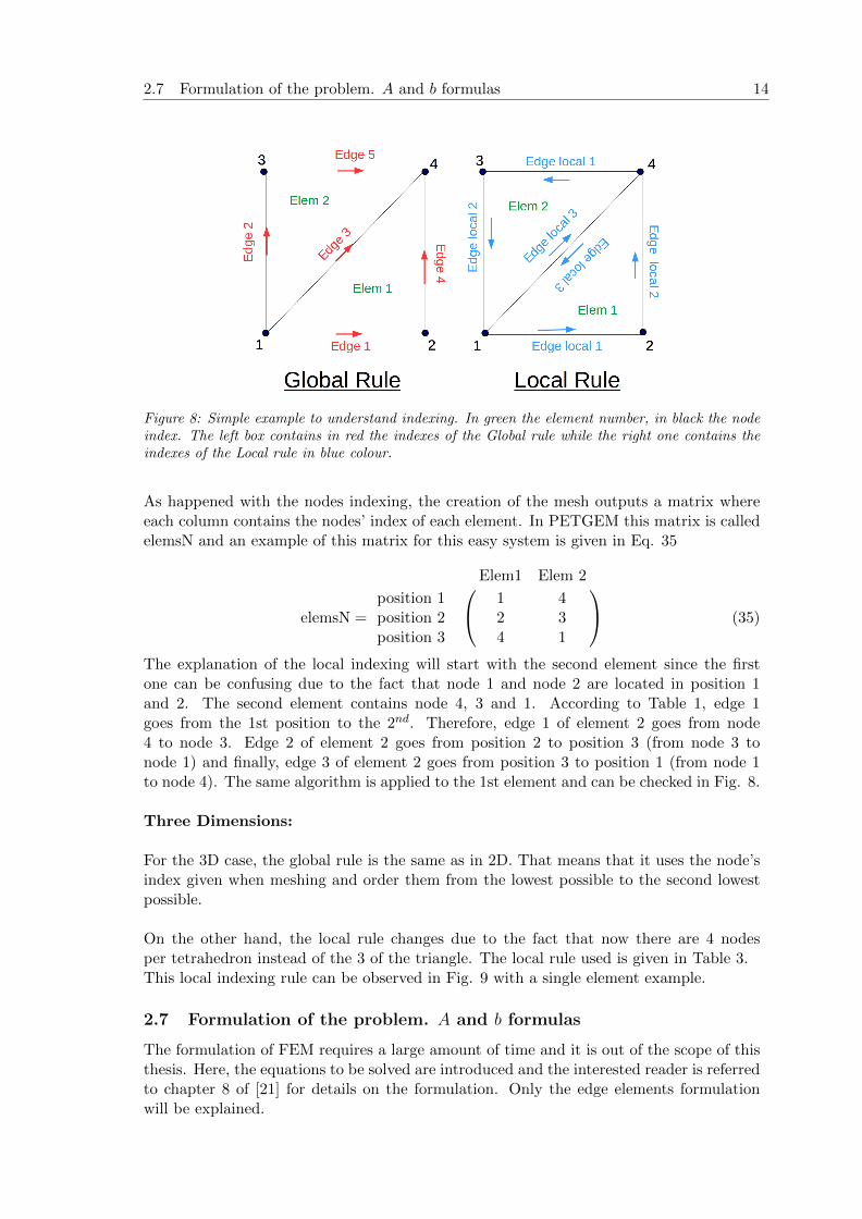
Figure 8: Simple example to understand indexing. In green the element number, in black the nodeindex. The left box contains in red the indexes of the Global rule while the right one contains theindexes of the Local rule in blue colour.

As happened with the nodes indexing, the creation of the mesh outputs a matrix whereeach column contains the nodes’ index of each element. In PETGEM this matrix is calledelemsN and an example of this matrix for this easy system is given in Eq. 35

elemsN =

Elem1 Elem 2

position 1 1 4position 2 2 3position 3 4 1

(35)

The explanation of the local indexing will start with the second element since the firstone can be confusing due to the fact that node 1 and node 2 are located in position 1and 2. The second element contains node 4, 3 and 1. According to Table 1, edge 1goes from the 1st position to the 2nd. Therefore, edge 1 of element 2 goes from node4 to node 3. Edge 2 of element 2 goes from position 2 to position 3 (from node 3 tonode 1) and finally, edge 3 of element 2 goes from position 3 to position 1 (from node 1to node 4). The same algorithm is applied to the 1st element and can be checked in Fig. 8.

Three Dimensions:

For the 3D case, the global rule is the same as in 2D. That means that it uses the node’sindex given when meshing and order them from the lowest possible to the second lowestpossible.

On the other hand, the local rule changes due to the fact that now there are 4 nodesper tetrahedron instead of the 3 of the triangle. The local rule used is given in Table 3.This local indexing rule can be observed in Fig. 9 with a single element example.

2.7 Formulation of the problem. A and b formulas

The formulation of FEM requires a large amount of time and it is out of the scope of thisthesis. Here, the equations to be solved are introduced and the interested reader is referredto chapter 8 of [21] for details on the formulation. Only the edge elements formulationwill be explained.

2.7 Formulation of the problem. A and b formulas 15

Table 3: Local indexing for 3D tetrahedra elements.

Edgei nodeinitial nodeend

1 1 22 1 33 1 44 2 35 4 26 3 4

Figure 9: Local indexing rule example in a single tetrahedron.

The best way to understand the formulation is by an example. The example used will bethe FEM formulation of the electromagnetic differential equation that PETGEM solveswhich is:

(∇×∇×+iwµσ) Es = −iwµ 4σ Ep (36)

The derivation of this formula and the interpretation of its parameters will be given inSection 3). The FEM formulation of this differential equation is given by:

(Kejk + iwµσM e

jk)︸ ︷︷ ︸A

{Eek}︸ ︷︷ ︸x

= −iwµ4σ{Rek}︸ ︷︷ ︸b

, (37)

where {Esk} is the vector of the DOFs, {Rek} is a vector that is integrated numerically,and Ke

jk and M ejk are called the Stiffness and the Mass matrix respectively. They have

different forms for the 2D and the 3D case as discussed in the following two paragraphs.

Two dimensional formulation:

In 2 dimensions, the stiffness and mass matrices are given by:

Keij =

∫∫we

(∇×Nei ) · (∇×Ne

j ) dS

M eij =

∫∫we

Nei ·Ne

j dS.

(38)

2.7 Formulation of the problem. A and b formulas 16

It is very important to note that the FEM formulation integrates the operators of the dif-ferential equation all over the domain. These two integrals can be computed analyticallyfor rectangular and triangular elements. However, they need to be computed numeri-cally for quadrilateral elements. For the triangular discretizations, these two integrals arecomputed by:

Keij =

lei lej

4e(39)

M e11 =

(le1)2

244e(m22 −m12 +m11)

M e22 =

(le2)2

244e(m33 −m23 +m22)

M e33 =

(le3)2

244e(m11 −m13 +m33)

M e21 = M e

12 =le1l

e2

484e(m23 −m22 − 2m13 +m12)

M e31 = M e

13 =le1l

e3

484e(m21 −m11 − 2m23 +m13)

M e32 = M e

23 =le2l

e3

484e(m31 −m33 − 2m12 +m23) ,

(40)

where mij = bei bej + cei c

ej . It is important to remark that these matrices are obtained for

each element e. Since the discretization is triangular, there are three edges per elementand therefore three DOFs per element. Consequently, the matrices are 3x3. The globalmatrix A is n x n where n is the total number of DOFs in the whole mesh. The computa-tion of the global matrix A is not trivial since the positions of the elements’ matrices mustbe allocated in the global matrix. The discussion of the building of the matrix A and thevector b will be given in the subsection 2.8.

Three dimensional formulation

Equivalent to the 2D case, in 3D the stiffness and mass matrices are given by:

Keij =

∫∫∫we

(∇×Nei ) · (∇×Ne

j ) dV

M eij =

∫∫∫we

Nei ·Ne

j dV.

(41)

For the tetrahedral elements that will be used in this thesis, the stiffness matrix is givenby:

Keij =

4lei lejV

e

(6V e)4[(cei1d

ei2 − cei2dei1)(cej1d

ej2 − cej2dej1)

(dei1bei2 − dei2bei1)(dej1b

ej2 − dej2bej1)(bei1c

ei2 − bei2cei1)(bej1c

ej2 − bej2cej1)].

(42)

The mass matrix for tetrahedral elements is now 6x6 since there are six edges (DOFs) perelement. There is no general formula to describe all 36 terms of the mass matrix but itcould be defined with 21 formulas. Those 21 formulas to describe M e

ij will not be writtenin this thesis because it is out of the scope but they can be found in page 301 of [21].

2.8 Assembly of A and b 17

2.8 Assembly of A and b

This subsection explains the assembly of the global matrix Aij from the Stiffness Keij and

Mass M eij matrices for each element; and the building of global array b from the numerical

integration of Rek. Both the building of A and b rely on the indexing rules that have beenset before. For a better understanding, the explanation will be started with the buildingof b. Moreover, all explanations will be only focused on the 2D case for its simplicity. The3D case can be extracted from the 2D.

b array

It is common to use an initial profile when solving a differential equation in FEM. This isthe case of PETGEM’s main equation:

(∇×∇×+iwµ(σ − σp)) Es︸︷︷︸Result of the computation

= −iwµ (σ − σp) Ep︸︷︷︸Initial Profile

The initial profile is always contained in the b array. As Keij and M e

ij are the operatorsintegrated over the whole domain, Rek of Eq. 36 is the integral over the whole domain ofEp. In fact, Rek is given by:

Rek =

∫∫we

Nek ·Ep. (43)

This integral can sometimes be computed analytically depending on the shape of Ep.However, for a general purpose, this integral will be done numerically using Gaussianquadrature [22]. The main idea behind Gaussian quadrature is to compute an integral ofa function as a sum of this function evaluated in some points multiplied by some weights.The choice of points to use and their weights rely on the shape of the integral domain.In this 2D case, the integrals are over triangles. The repository [22] provides a large setof Gaussian points locations (ri), it’s weights (weight(i)) and the formula to transformthe locations from a unit triangle to any arbitrary triangle. Introducing the Gaussianquadrature approximation, Rek becomes:

Rek =

∫∫we

Nek ·Ep '

# Guass Points∑i=1

weight(i) Nek(ri) ·Ep(ri) (44)

Once these computations are finished, Rek is obtained where e is the index of the elementand k = 1, 2, 3 is the index of the DOF (edge). Following the specific problem that is beingsolved, it is defined bek ≡ −iwµ (σ − σp)Rek.

Now, bek can be computed for all e and k. However this elements must be allocatedin the global array b. In order to get a better understanding of the allocation process, thesimple example used in the indexing section (Fig. 8) will be used as well. The allocationprocess depends on the local indexing and, also, on a variable not mentioned yet calledEdgesN. This variable and elemsN (Eq. 35) are part obtained on the Preprocessing ofthe Mesh as it will be explained later. The information needed to allocate this specificproblem is contained in Fig. 10:

This figure exemplifies the allocation process of bek in the global array b. It is importantto remark that since the mesh is based on 2 elements and 5 edges, the global array b will

2.8 Assembly of A and b 18

Figure 10: On the left side, the local indexing of the easy example. On the right side, the allocationprocess with the matrix edgesN highlighted in yellow.

have 5 components. This is a general rule, the length of b is the number of DOFs. Startingfrom the 1st element, the left figure shows that the first edge goes from node 1 to node 2.Looking on the edgesN matrix, from 1 to 2 corresponds to the global edge 1. Therefore, b11goes with a + sign to the first position of the global array b. The + sign is due to the factthat both the local and the global indexing go from 1 to 2. If one went from 1 to 2 and theother from 2 to 1 it would correspond a - sign. The second edge of the first element goeslocally from 2 to 4 and it corresponds in the matrix edgesN to the 4th position. Therefore,b12 goes to the 4th position of b with a + sign. The 3rd edge of the 1st element goes fromnode 4 to node 1. The 3rd position of edgesN goes from 1 to 4. In this case, one is from 1to 4 and the other is from 4 to 1. Therefore, b13 goes to the the 3rd position of b with a -sign. Once the first element is finished, it is time for the second and last element. Its 1st

edge goes from 4 to 3 and the 5th position of edgesN goes from 3 to 4. Therefore, b21 goesto the 5th position with a - sign. The second edge goes from 3 to 1 that corresponds tothe second position of edgesN that is from 1 to 3. Therefore, b22 goes to the 2nd positionwith a - sign. Finally, edge 3 goes from 1 to 4 as the 3rd position of edgesN. Therefore, b23is added with a + sign to the −b13 that was already in the 3rd position of edgesN.

Matrix A

To sum up, the equation that follows the stiffness matrix (Keij) for 2D is in Eq. 39

and in 3D in Eq. 41. Moreover, the mass matrix (M eij) follows in 2D Eq. 40 and in 3D is

given in page 301 of [21]. Once Keij and M e

ij can be computed for both 2D and 3D, Aeij isobtained using Eq. 45:

Aeij = Keij + iwµ(σ − σp)M e

ij (45)

Once Aeij is known for every element, it is time to allocate this matrices in the globalmatrix A that is a squared matrix with dimension number of edges (DOFs). As happenedwith the assembly of b, the signs of the elements must be taken into account. In theassembly of A is easier to include the signs just before the allocation and to do so it isrequired the function Signs given in Eq. 46

Sei =nodeei2 − nodeei1|nodeei2 − nodeei1|

(46)

where i is the edge index that joins nodeei1 with nodeei1 of the element e. Afterwards, aeij

2.8 Assembly of A and b 19

is defined as the element that will be allocated containing the signs analysis that is givenby:

aeij = AeijSei S

ej (47)

In order to allocate aeij , a matrix called connectivity (will be shorted to “elemsE”) isneeded. This matrix specifies which edges belong to each element and it is very similar tothe matrix elemsN that was introduced before in Eq. 35. The computation of “elemsE”is out of the scope of this thesis but for the two-triangles example, this matrix is:

elemsE =

Elem1 Elem 2

position 1 1 5position 2 4 2position 3 3 3

(48)

Firstly, the general rule will be given and then it will be exemplified using the two-trianglesexample. Defining the column e of the matrix “elemsE” as (k, l,m), then the coefficientaeij is allocated following the rule:

a11 → (k, k) a12 → (k, l) a11 → (k,m)

a21 → (l, k) a22 → (l, l) a23 → (l,m)

a31 → (m, k) a32 → (m, l) a33 → (m,m)

Assuming that for this example the matrices a1 and a2 for each element are given by:

a1 =

λ11 λ12 λ13

λ21 λ22 λ23

λ31 λ32 λ33

a2 =

Λ11 Λ12 Λ13

Λ21 Λ22 Λ23

Λ31 Λ32 Λ33

(49)

The column 1 of “elemsE” is (1, 4, 3) and the second column is (5, 2, 3). Therefore, theallocation of this problem is the following one:

A =

λ11 0 λ13 λ12 00 Λ22 Λ23 0 Λ21

λ31 Λ32 λ33 + Λ33 λ32 Λ31

λ21 0 λ23 λ22 00 Λ12 Λ13 0 Λ11

(50)

Knowing A and b, one can solve the equation A·x = b by inverting the matrix A: x = A−1b.The most important requirement is that the determinant of a matrix must be differentto zero in order to be able to invert that matrix (det(A) 6= 0). There are many differentmethods to numerically invert a matrix and which one to use depends on the matrix itself.However, this topic is out of the scope of the thesis and no further information will beaddressed.

3 PETGEM 20

3 PETGEM

3.1 Brief description of PETGEM

The Parallel Edge-based Tool for Geophysical Electromagnetic Modelling (PETGEM) isa Python HPC scalable tool based on the finite element method. This code contains morethan 8000 lines with many different modules such as the preprocessing, the assembly,the solver, the postprocessing, ... PETGEM has been developed as open-source (underGPLv3 license) at the Department of Computer Applications in Science & Engineering(CASE) of the Barcelona Supercomputing Center (BSC). PETGEM solves the marineControlled-Source Electromagnetic method (CSEM) which is an important technique forreducing ambiguities in data interpretation for hydrocarbon exploration. In order to solveCSEM, one must solve Maxwell’s equations 51 where the harmonic time dependence e−iwt

is omitted.

∇×E = iwµ0H ∇×H = Js + σE , (51)

where w is the frequency, σ the conductivity and Js the distribution of source currentwhich is considered a punctual source. Using a perturbation approach, the total electricfield is written as a sum of a primary field (the known term) and a secondary field (the partthat will be computed) E = Es + Ep. For a general layered Earth model, Ep is computedusing a Hankel transform filters [23].

The same procedure can be applied to electric conductivity. Following the common geo-physics notation, σ = σs +4σ, where 4σ is the electrical conductivity of the area wherethe focus is located. Therefore, σs will change along the sediments. On the focus zone itwill be 0 and on the other zones will be given by σs = σreal −4σ. One can get the finalequation to solve:

∇×∇×Es + iwµ0σEs = −iwµ0 4σ Ep (52)

PETGEM is an HPC code due to the fact that edge elements offer a good scalability andit is exploited through the Python Package Petsc4py [24].

3.2 How to use PETGEM

In order to install PETGEM, one must follow the guide [25]. On the following paragraphs,a guide to understand PETGEM is given. Those instructions are the result of the learningprocess of the multiple simulations carried out using this code. The tutorial is divided in:preprocessing, kernel and visualization of the output.

3.2.1 Preprocessing

In order to run the preprocessing, one needs to prepare a file called “preprocessing-Params.py”. An example of this file is found below:

preprocessing = {

# ---------- Mesh file ----------

’MESH_FILE’: ’/home/marc/Dropbox/BSC/gmsh/cube/cube.msh’,

# ---------- Material conductivities ----------

’MATERIAL_CONDUCTIVITIES’: [1.0],

3.2 How to use PETGEM 21

# ---------- Receivers position file ----------

’RECEIVERS_FILE’: ’/home/marc/Dropbox/BSC/gmsh/cube/cube.txt’,

# ---------- Path for Output ----------

’OUT_DIR’: ’/home/marc/petgem-0.30.43/PreprocessingOutput/’,

}

The four elements needed are now introduced. The first one is the mesh file which hasalready been explained how to create it. The second element is the material conductivities.This part of the code is important to solve geophysical problems where there are differentlayers with different conductivities but for this thesis, the plasma will be considered tohave a homogeneous conductivity of 1.0 from now on. The third option is the Receiversfile which must be a txt containing the X, Y and Z coordinates of each element separatedby a tab. The following example contains just 3 receivers:

0.000 0.000 0.000

1.000 0.000 0.000

0.000 1.000 0.000

On appendix C there are two Matlab algorithms to create homogeneous distributions ofreceivers for both a cube and a cylinder. Finally, the last variable needed is the outputdirectory where there will be stored the code output’s.

Once the file “preprocessingParams.py” is ready, it is time to execute the file “run pre-processing.py”. To do so, one must execute on the computer’s console:

python3 /....../run_preprocessing.py /....../preprocessingParams.py

where /....../ refers to specify the folder where those files are.

3.2.2 Kernel

The file “kernel.py” also requires of two auxiliary parameters files called “pets.ops” and“modelParams.py”. The first one contains parameters of the solution which are out ofthe scope of this thesis but further information can be found on [26]. The second file isvery similar to “preprocessingParams.py”. It contains variables that will be used in thecomputations. Those variables can be separated into two groups: the ones that define Epand the ones related to the mesh. The elements in the second subgroup are the output ofthe preprocessing. Finally, to run the kernel one must write on the console:

mpirun -n X python3 /....../kernel.py -options_file /....../petsc.opts

/....../modelParams.py

where /....../ refers to specify the folder where those files are and X the numbers of coreswhere the job will be parallelized.

3.2.3 Visualization

PETGEM does not give the visualization by itself. However, it generates output files withthe electric responses at receivers positions available in the formats ASCII, PETSc andMatlab. Appendix C contains a simple Matlab script created in this thesis work in orderto view the output of PETGEM.

4 Results 22

4 Results

The thesis work consists of following four steps: to understand and learn EFEM theory,to understand the workflow and the scripts of PETGEM code, to check the capability toimplement different initial profiles to PETGEM and to change the equations that PET-GEM solves and introducing the time integration of the equations as summarized in thischapter:

Learn EFEM→ Understanding PETGEM→ Check initial profile→ Change equations

The most time demanding part of this thesis is understanding and being able to modifyPETGEM because it is an HPC code with more than 8000 lines and many different modulessuch as the preprocessing, the assembly, the solver, the postprocessing, ... That is why thiscurrent thesis has stopped at the changing equations steps, where some research has beendone but none remarkable result of changing the equations has been achieved. However,there has been many important results and achievements that will be described in thefollowing lines.

4.1 FEM Mesh Creation

The finite element method mesh must be created using Gmsh [27]. This software is open-source and it can be used both with its graphic interface or via script-console. A 2Dexample of a rectangular mesh generation using Gmsh is given in the following lines.

lc=0.1; //radius length of vertex

//Point(i) = {x, y, z, radius of the vertex};

Point(1) = {0, 0, 0, lc};

Point(2) = {1, 0, 0, lc} ;

Point(3) = {1, 3, 0, lc} ;

Point(4) = {0, 3, 0, lc} ;

//Line(k) = {i,j}; From point i to j.

Line(1) = {1,2} ;

Line(2) = {3,2} ;

Line(3) = {3,4} ;

Line(4) = {4,1} ;

//Line Loop Closes the area.

Line Loop(1) = {4,1,-2,3} ;

//minus since line2 is 3-2 and not 2-3

Plane Surface(1) = {1} ;

This code only creates the geometry to be divided in elements. To create the mesh click onModules>Mesh>Define>2D (or 3D for those geometries). By default, this configurationcreates meshes with triangular, hexahedra, pyramid, ... elements. In order to make themesh only with a specific type of elements, one must go to Tools>Options>Mesh>elementsand unselect all except the one wanted.

As it has been mentioned before, the refinement process is an important step to optimizethis method. Gmsh documentation provides a detailed tutorial on different strategies torefine a mesh [28]. Appendix A provides an example of refinements over a point, a line

4.1 FEM Mesh Creation 23

(a) (b)

(c) (d)

(e) (f)

(g) (h).

Figure 11: Set of different geometries obtained using Gmsh. The left panels are the homogeneousmeshes while the right ones are the refined meshes.

and a box. On https://github.com/marcfusterr/Gmsh_Scripts there are uploadeddifferent codes to generate 2D geometries (circle and square) and 3D geometries (cylinderand cube) developed in this thesis work. All codes have both a homogeneous and a refinedmesh. Figure 11 shows two cases of the distribution of the mesh density; homogeneous and

4.2 Implementation of initial profile 24

inhomogeneous in the simulation volume. They are plotted from PETGEM output datausing the Gmsh graphic interface. The work contributes to the visualization of the datausing Paraview [29] so that the GUI analysis can be made directly from the visualization.The capability of the arbitral choice of the mesh density concentration cases the simulationsaccording to the physics problems to be solved.

4.2 Implementation of initial profile

Before studying the feasibility of applying PETGEM to plasma physics, the ability to im-plement initial profiles to PETGEM must be checked. This subsection contains a bench-mark of the implementation of an initial profile and also explains how to get the velocityfield from the velocity potential.

4.2.1 Benchmark

The implementation of an initial profile is not a trivial task in PETGEM. That is be-cause PETGEM always uses the same initial profile: the electric field created from CSEMantenna using the Hankel filters mentioned before. Therefore, the code is not preparedfor the initial profile to be changed. Changing the initial profile in PETGEM requiresintroducing the function to be implemented in both the “postprocessing.py” and “assem-bler.py”. Moreover, the choice of an initial profile must go with a choice of a good set ofreceivers in order to correctly appreciate the output.

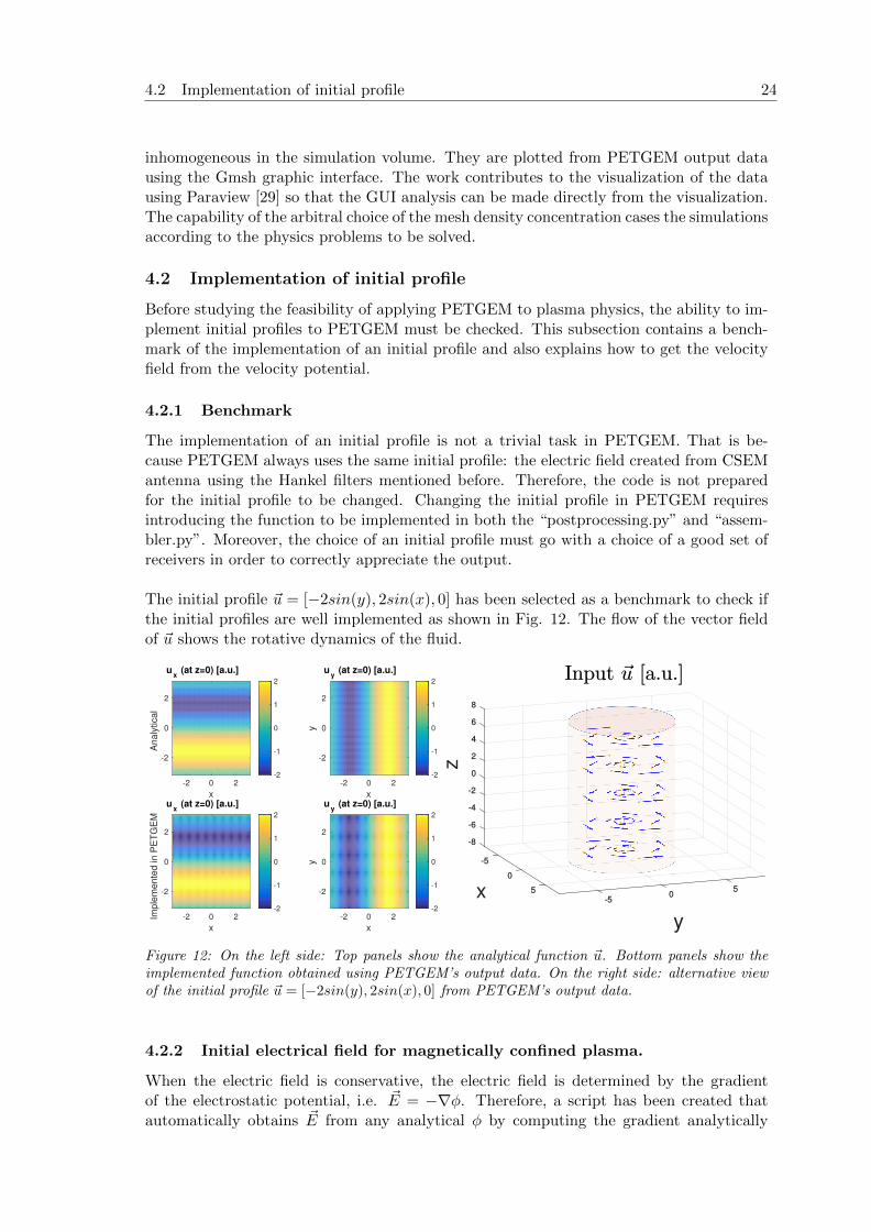
The initial profile ~u = [−2sin(y), 2sin(x), 0] has been selected as a benchmark to check ifthe initial profiles are well implemented as shown in Fig. 12. The flow of the vector fieldof ~u shows the rotative dynamics of the fluid.

x

-2 0 2

An

aly

tica

l

-2

0

2

ux (at z=0) [a.u.]

-2

-1

0

1

2

x

-2 0 2

y

-2

0

2

uy (at z=0) [a.u.]

-2

-1

0

1

2

x

-2 0 2Imp

lem

en

ted

in

PE

TG

EM

-2

0

2

ux (at z=0) [a.u.]

-2

-1

0

1

2

x

-2 0 2

y

-2

0

2

uy (at z=0) [a.u.]

-2

-1

0

1

2

Figure 12: On the left side: Top panels show the analytical function ~u. Bottom panels show theimplemented function obtained using PETGEM’s output data. On the right side: alternative viewof the initial profile ~u = [−2sin(y), 2sin(x), 0] from PETGEM’s output data.

4.2.2 Initial electrical field for magnetically confined plasma.

When the electric field is conservative, the electric field is determined by the gradientof the electrostatic potential, i.e. ~E = −∇φ. Therefore, a script has been created thatautomatically obtains ~E from any analytical φ by computing the gradient analytically

4.3 Steady state plasma 25

using the Python package Sympy [30]. The cylindrical geometry is used in mirror plasmaconfinement devices such as SLPM [31], PANTA [32], etc. The plasma confined in thecylindrical geometry is a useful approach to study the plasma instabilities. The densityof the simulation grid can be arbitrarily chosen in the simulation domain. The locationof the mesh concentration can be chosen depending on the physics problem to be aimedto study. Figure 13 shows the electric field obtained from φ = exp(−(x/1.5)2 − (y/1.5)2))using the automatic gradient script.

3

5

7

9

10

2

4

6

8

Figure 13: On the right hand, output of the automatic gradient script obtained from the electricpotential φ = exp(−(x/1.5)2 − (y/1.5)2) which is plotted on the left part.

4.3 Steady state plasma

The full wave equation in a magnetically confined plasma with an antenna current as aboundary condition is given by Eq. 53:

∇×∇×E− w2

c2E =

4πwi

c2(Jp + Ja)

Jp(r) =

∫dr′σ(r, r′)E(r′)

(53)

where Ja is the current of the antenna and σ is the conductivity tensor. This equationhas the same shape as the one that PETGEM solves. However, this equation is thewave equation with a boundary condition corresponding to the current density introducedby the antenna while Eq. 52 is the perturbation solution of a wave propagating in theearth. Figure 14 shows the initial profile of the current density J = Jp + Ja = z/f(r)along with it’s electrical response, where f(r) = (1 + (r/a)2Λ)1+1/Λ and a = 0.25m is theradius of the cylinder and Λ = 4 [33]. The implemented current profile is a reasonableapproach to compute the initial profile of the current density and the electric field for fusionplasmas [34]. The time variation of the current density will be implemented in the futurein order to investigate the interactions between the effect of the antenna and the plasmaresponse. The output ~E which is solved from ~J can be obtained by PETGEM calculation.However the initial profile implemented here is time-independent quantity, and it does nothave a function of the coefficient of the time-frequency. The PETGEM output ~E showszero (or numerical noise). It is as expected and it confirms the implementation and thePETGEM calculation have been performed correctly without generating any unexpectederrors.

4.3 Steady state plasma 26

Figure 14: Initial profile of the antenna current density to be solved by the full wave equation.

5 Conclusions 27

5 Conclusions

The study of the assessment of this new research line of the EFEM application to fusionplasma physics has been successfully carried out. Due to the complex dynamics of theplasma, high performance simulations are required. Therefore, this work demonstratesthe capability to perform and modify a large parallel code in the supercomputer Marenos-trum. The edge finite element method theory has been studied and has been found tobe more useful than the nodal finite element method for electromagnetic problems andtherefore, for fusion problems.

Moreover, this work demonstrates the generation of the simulation mesh for finite el-ement method for fusion plasma in the different geometries such as squares, circles,cubes and cylinders. The location and the density of the mesh concentration can bearbitrarily adopted according to the physics problem which is aimed to investigate ina user-friendly manner using the codes that have been uploaded to the Github linkhttps://github.com/marcfusterr/Gmsh_Scripts. The implementation of the initialfield of any quantities such as electric field, and the application of the reasonable currentprofile which is specifically aimed for the fusion plasma research have been carried out.

6 Future Work 28

6 Future Work

The future steps of the work are to go beyond the calculation of the steady state plasmaand implement the time integration of the plasma dynamics. The long-term objective is tosolve the magnetohydrodynamic (MHD) which is the combination of the electromagnetismsystem i.e. Maxwell’s equations and the fluid system i.e. Navier-Stokes equation. Theprimitive approach is to develop the fluid modeling part considering an incompressible(∇ · u = 0), diffusive model: ∂u

∂t = −ν ∇×∇× u which is ongoing to be implemented inPETGEM. Once the diffusive model is finished, Navier-Stokes equation should be imple-mented and, afterward, MHD equations. The development team of PETGEM is currentlyintroducing a more complex numerical scheme, the higher order elements. This schemeconsists of polynomial interpolation functions rather than linear interpolation functions.Therefore, an important future step is to adapt all the work done to the new PETGEMscheme.

REFERENCES 29

References

[1] I.P. Mysovskikh. Trapezium formula. https://www.encyclopediaofmath.org/index.php/

Trapezium_formula.

[2] I.P. Mysovskikh. Romberg method. https://www.encyclopediaofmath.org/index.php/

Romberg_method.

[3] http://ourfiniteworld.com/2012/03/12/world-energy-consumption-since-1820/.

[4] http://nupex.eu/index.php?g=textcontent/nuclearenergy/nuclearfusion&lang=en.

[5] F.F. Chen. Introduction to Plasma Physics and Controlled Fusion. Number v. 1 in Introductionto Plasma Physics and Controlled Fusion. Springer, 1984.

[6] E. Stuhlinger. Ion propulsion for space flight. McGraw-Hill New York, 1964.

[7] I-H. Loh and M.S. Sheu. Plasma surface modification in biomedical applications. MRS OnlineProceedings Library Archive, 414, 1995.

[8] V.L. Bonch-Bruevich and Sh.M. Kogan. The theory of electron plasma in semiconductors.Soviet Phys.-Solid State, 1, 1960.

[9] K. Miyamoto. Plasma physics for nuclear fusion. MIT Press, 1989.

[10] B.D. Bondarenko. Role played by o a lavrent’ev in the formulation of the problem and theinitiation of research into controlled nuclear fusion in the ussr. Physics-Uspekhi, 44(8):844,2001.

[11] http://www.sciencedirect.com/science/article/pii/S2468080X1630032.

[12] E. Hill. Physics of fusion power lecture 6: Conserved quantities / mirror device / tokamak.http://slideplayer.com/slide/4645450/.

[13] Iter webpage. https://www.iter.org/.

[14] G. Huijsmans and O. Czarny. Mhd stability in x-point geometry: Simulation of elms. 47:659,06 2007.

[15] L.G. Eriksson et al. Comparison of time dependent simulations with experiments in ioncyclotron heated plasmas. Nuclear Fusion, 33(7):1037, 1993.

[16] T. Kurki-Suonio et al. Ascot simulations of fast ion power loads to the plasma-facing compo-nents in iter. Nuclear Fusion, 49(9):095001, 2009.

[17] R. Kleiber and R. Hatzky. Euterpe gyrokinetic code. http://fusionwiki.ciemat.es/wiki/EUTERPE.

[18] O. Castillo-Reyes. Parallel edge-based tool for geophysical electromagnetic modelling (pet-gem). http://petgem.bsc.es/.

[19] R. Nicoletti. Comparison between a meshless method and the finite differencemethod for solving the reynolds equation in finite bearings. 2013;135(4):044501-044501-9.doi:10.1115/1.4024752. ASME. J. Tribol.

[20] G. Mur. Edge elements, their advantages and their disadvantages. IEEE Transactions onMagnetics, 30 (5), 30, 09 1994.

[21] J.M. Jin. The finite element method in electromagnetics. John Wiley & Sons, 2015.

[22] Repository of quadrature rules for triangles. https://people.sc.fsu.edu/~jburkardt/

datasets/quadrature_rules_tri/quadrature_rules_tri.html.

[23] F.N. Kong. Hankel transform filters for dipole antenna radiation in a conductive medium.Geophysical Prospecting, 55(1):83–89, 1960.

[24] L.D. Dalcin et. al. Parallel distributed computing using python. Advances in Water Resources,34(9):1124 – 1139, 2011. New Computational Methods and Software Tools.

REFERENCES 30

[25] O. Castillo-Reyes. Petgem installation guide. https://pypi.org/project/petgem/.

[26] S. Balay et al. PETSc Web page. http://www.mcs.anl.gov/petsc, 2017.

[27] C. Geuzaine and J-F. Remacle. Gmsh. http://gmsh.info/.

[28] C. Geuzaine. Gmsh refining tutorial. https://gitlab.onelab.info/gmsh/gmsh/blob/

master/tutorial/t10.geo.

[29] A. Henderson. Paraview guide, a parallel visualization application. Kitware Inc., 2007.

[30] A. Meurer. Sympy: symbolic computing in python. PeerJ Computer Science, 3:e103, January2017.

[31] F. Castellanos et al. Parallel flows and turbulence in a linear plasma machine. Plasma Physicsand Controlled Fusion, 47(11):2067, 2005.

[32] S. Inagaki et al. A concept of cross-ferroic plasma turbulence. Scientific Reports, 6:22189, 022016.

[33] X. Shan and D. Montgomery. On the role of the hartmann number in magnetohydrodynamicactivity. Plasma Physics and Controlled Fusion, 35(5):619, 1993.

[34] S. Futatani J. Morales and W.J.T. Bos. Dynamic equilibria and magnetohydrodynamic in-stabilities in toroidal plasmas with non-uniform transport coefficients. Physics of Plasmas,22:052503.

A 3D Mesh creation and Refinement 31

A 3D Mesh creation and Refinement

This code summarizes how to create geometries (points, lines, surfaces and volumes) andhow to create an inhomogeneous mesh by refining over points, lines, surfaces and volumes.With those basic geometries, one can adapt them to create different objects.

lc=0.1; //radius length of vertex

// lower surface

Point(1) = {0, 0, 0, lc};

Point(2) = {1, 0, 0, lc} ;

Point(3) = {0, 1, 0, lc} ;

Point(4) = {1, 1, 0, lc} ;

Line(1) = {1,2} ;

Line(2) = {2,4} ;

Line(3) = {4,3} ;

Line(4) = {3,1} ;

Line Loop(1) = {1,2,3,4} ;

// minus since line2 is 3-2 and not 2-3

Plane Surface(1) = {1} ;

//uper surface

Point(5) = {0, 0, 1, lc};

Point(6) = {1, 0, 1, lc} ;

Point(7) = {0, 1, 1, lc} ;

Point(8) = {1, 1, 1, lc} ;

Line(5) = {5,6} ;

Line(6) = {6,8} ;

Line(7) = {8,7} ;

Line(8) = {7,5} ;

Line Loop(2) = {5,6,7,8} ;

// minus since line2 is 3-2 and not 2-3

Plane Surface(2) = {2} ;

//join both surface

Line(9) = {1,5} ;

Line(10) = {2,6} ;

Line(11) = {3,7} ;

Line(12) = {4,8} ;

Line Loop(3) = {9,5,-10,-1}; Plane Surface(3) = {3};

Line Loop(4) = {2,12,-6,-10}; Plane Surface(4) = {4};

Line Loop(5) = {3,11,-7,-12}; Plane Surface(5) = {5};

Line Loop(6) = {-4,11,8,-9}; Plane Surface(6) = {6};

Surface Loop(100) = {1,2,3,4,5,6};

Volume(101) = {100};

Physical Volume ("Seds", 1) = {101}; // This line is necessary for

// PETGEM in order to understand each layer.

B Algorithm’s to create a homogeneous distribution of receivers 32

// #################################################################

// # Refine a Point and or a line #

// #################################################################

// points to increase density

Point (11) = {0.5,1,0.5,lc};

Field[1] = Attractor;

//list of the points where to have a higher density

Field[1].NodesList = {11};

//list of lines where to have a higher density

Field[1].EdgesList = {9};

Field[2] = Threshold;

Field[2].IField = 1;

Field[2].LcMin = lc / 10.;

Field[2].LcMax = lc;

Field[2].DistMin = lc / 4.;

Field[2].DistMax = 2.*lc;

// #################################################################

// # Refine a rectangle and or a solid box #

// #################################################################

Field[3] = Box;

Field[3].VIn = lc / 10;

Field[3].VOut = lc;

Field[3].XMin = 0.25;

Field[3].XMax = 0.75;

Field[3].YMin = 0.25;

Field[3].YMax = 0.75;

Field[3].ZMin = 1.;

Field[3].ZMax = 1.;

//by setting Min=Max in 1 dimension, we get a rectangle

//if for all dimensions Min different Max, one gets

//a solid cube

// #################################################################

// # Join all Fields #

// #################################################################

// Use minimum of all the fields as the background field

Field[11] = Min;

Field[11].FieldsList = {2,3};

Background Field = 11;

B Algorithm’s to create a homogeneous distribution of re-ceivers

The first algorithm is used to create an homogeneous distribution of receivers in a unitarybox from -0.4 to 0.4 in all directions. To scale the receivers just change the variable

B Algorithm’s to create a homogeneous distribution of receivers 33

ScaleFactor.

ScaleFactor=100;

xtarget=[0.1:0.1:0.9];

ytarget=[0.1*ones(1,9)];

for irepeat=1:8

xtarget=[xtarget,0.1:0.1:0.9];

ytarget=[ytarget,0.1*(irepeat+1)*ones(1,9)];

end

[a,lengthxtarget]=size(xtarget);

xtarget2=xtarget;

ytarget2=ytarget;

ztarget2=0.1*ones(1,lengthxtarget);

for irepeat=1:8

xtarget2=[xtarget2,xtarget];

ytarget2=[ytarget2,ytarget];

ztarget2=[ztarget2,0.1*(irepeat+1)*ones(1,lengthxtarget)];

end

[a,lengthxtarget2]=size(xtarget2);

receivers = zeros(lengthxtarget2, 3);

receivers(:,1)=xtarget2-0.5;

receivers(:,2)=ytarget2-0.5;

receivers(:,3)=ztarget2-0.5;

receivers=ScaleFactor*receivers;

dlmwrite(’/home/marc/Dropbox/BSC/gmsh/cube/cube.txt’,...

receivers,’delimiter’,’\t’,’precision’,’%.6e’)

The second one is equivalent but for a cylinder. “R” changes the radius, “L” the lengthand “n” the number of layers of receivers in the Z direction

R=23/100;

L=96/100;

n=5;

xtargetAux=R*[1,0.5,0.5,0,0,0,-0.5,-0.5,-1,0.25,0.25,-0.25,...

-0.25,0.15,0.15,-0.15,-0.15,0,0,0.25,-0.25];

ytargetAux=R*[0,0.5,-0.5,1,0,-1,0.5,-0.5,0,0.25,-0.25,0.25,...

-0.25,0.15,-0.15,0.15,-0.15,0.25,-0.25,0,0];

[nothing,lengthAux]=size(xtargetAux);

zdiv=linspace(0,L,n);

zAux=ones(1,lengthAux);

xtarget=xtargetAux;

ytarget=ytargetAux;

ztarget=zeros(1,lengthAux);

for i=1:n-1

xtarget=[xtarget,xtargetAux];

ytarget=[ytarget,ytargetAux];

ztarget=[ztarget,zAux*zdiv(i+1)];

end

[a,lengthtargets]=size(xtarget);

receivers = zeros(lengthtargets, 3);

receivers(:,1)=xtarget;

receivers(:,2)=ytarget;

receivers(:,3)=ztarget-L/2;

dlmwrite(’/home/marc/Dropbox/BSC/gmsh/cylinder/cylinder.txt’,...

receivers,’delimiter’,’\t’,’precision’,’%.6e’)

C Visualization Matlab script 34

C Visualization Matlab script

load(’/home/marc/petgem-0.30.48/examples/Output/Matlab/Ep.mat’);

load(’/home/marc/petgem-0.30.48/examples/Output/Matlab/Es.mat’);

load(’/home/marc/petgem-0.30.48/examples/Output/Matlab/Et.mat’);

receivers=load(’/home/marc/petgem-0.30.48/PreprocessingOutput/receiversPETGEM.txt’);

figure

quiver3(receivers(:,1), receivers(:,2), receivers(:,3),

real(Ep(:,1)),real(Ep(:,2)),real(Ep(:,3)))

hold on

scatter3(receivers(:,1), receivers(:,2), receivers(:,3),’.’)

hold off