Kovács, Sz., Kóczy, L.T.: Application of the Approximate Fuzzy Reasoning Based on Interpolation in the Vague Environment of the Fuzzy Rulebase in the Fuzzy Logic Controlled Path Tracking Strategy of Differential Steered AGVs, Computational Intelligence - Theory and Applications, Lecture Notes in Computer Science, 1226, Springer, pp.456-467, Germany, (1997). – Draft version.

Application of the Approximate Fuzzy Reasoning Based on Interpolation in the Vague Environment of the Fuzzy Rulebase in

the Fuzzy Logic Controlled Path Tracking Strategy of Differential Steered AGVs

Szilveszter Kovács

Computer Centre, University of Miskolc Miskolc-Egyetemváros, Miskolc, H-3515, Hungary

e-mail: szkszilv@gold.uni-miskolc.hu

László T. Kóczy

Department of Telecommunication an Telematics, Technical University of Budapest

Sztoczek u.2, Budapest, H-1111, Hungary

Abstract. In most of the practical applications the concept of vague environment [1] gives a simple way for fuzzy approximate reasoning. If the fuzzy partitions (used as primary sets of the fuzzy rulebase) can be described by vague environments [1], the primary fuzzy sets of the antecedent and the consequent parts of the fuzzy rules can be characterised by points in their vague environments. So the fuzzy rules themselves can be characterised by points in their vague environment too. It means, that the question of approximate fuzzy reasoning can be reduced to the problem of interpolation of the rule points in the vague environment of the fuzzy rulebase relation [2,3]. In this paper an approximate fuzzy reasoning method based on rational interpolation in the vague environment of the fuzzy rulebase will be introduced, and as an example of a practical application of the method, a path tracking control strategy for differential steered AGVs (Automated Guided Vehicle) [4] implemented on such a fuzzy logic controller will be introduced.

1 The Vague Environment and the Fuzzy Partition The concept of vague environment is based on the similarity or indistinguishability of the elements. Two values in the vague environment are ε-distinguishable if their distance is grater then ε. The distances in vague environment are weighted distances. The weighting factor or function is called scaling function (or factor) [1]. For finding connections between fuzzy sets and a vague environment we can introduce the membership function µ A x( ) as a level of similarity a to x, as the degree to which x is indistinguishable to a [1]. So the α-cuts of the fuzzy set µ A x( ) is the set which contains the elements that are (1−α)-indistinguishable from a (see fig.1.):

δ αs ( , )a b ≤ −1 ,

{ } ( )µ δA sx s x dx( ) min ( , ), min ,= − = −

∫1 1 1 1a ba

b

where δ s ( , )a b is the vague distance of the values a, b, and s(x) are the scaling function of the universe X.

Fig. 1.

It is very easy to realize (see fig.1.), that this case the vague distance of points a and b (δ s ( , )a b ) is basically the Disconsistency Measure (SD) of the fuzzy sets A and B (where B is a singleton):

( )S xDx X

A B s= − =∈

∩1 sup ( , )µ δ a b if [ ]δ s ( , ) ,a b ∈ 0 1

where A B∩ is the min t-norm, ( ) ( ) ( )[ ]µ µ µA B A Bx x x∩ = min , ∀ x ∈ X.

The main difference between the disconsistency measure and the vague distance is, that the vague distance is a crisp value in range of [0,∞], while the disconsistency measure is limited to [0,1]. That is why it is useful in interpolate reasoning with insufficient evidence too. So if it is possible to describe all the fuzzy partitions of the primary fuzzy sets (the antecedent and consequent universes) of our fuzzy rulebase, and the observation is a singleton, we can calculate the “extended” disconsistency measures of the antecedent primary fuzzy sets of the rulebase and the observation, and the “extended” disconsistency measures of the consequent primary fuzzy sets and the consequence (we are looking for) as vague distances of points in the antecedent and consequent vague universes. For generating a vague environment of a fuzzy partition we have to find an appropriate scaling function, which describes the shapes of all the terms in the fuzzy partition. A fuzzy partition can be characterised by a vague environment if and only if the membership functions of the terms fulfills the following requirement [1]:

s x xddx

( ) '( )= =µµ exists iff { }min ( ), ( ) ' ( ) ' ( )µ µ µ µi j i jx x x x> 0 ⇒ = ∀ ∈i j I, ,

where s(x) is the vague environment we are looking for. Generally the above condition is not fulfilling, so the question is how to describe all fuzzy sets of the fuzzy partition with one “universal” scaling function. For this reason we propose to use the approximate scaling function [2,3]. The approximate scaling function is an approximation of the scaling functions describes the terms of the fuzzy partition separately. Supposing that the fuzzy terms are triangles, each fuzzy term can be characterised by two constant scaling functions, the scaling factor of the left and the right slope of the triangle. So a triangle shaped fuzzy term can be characterised by three values (by a triple), by the values of the left and the right scaling factors and the value of its core

point (e.g., fig.2.). For generating the approximate scaling function we suggest to interpolate the neighbouring scaling factors (e.g., fig.2.).

The original fuzzy partition The approximate scaling function

The partition is characterised by two triple The approximate fuzzy partition

Fig. 2. Approximate scaling function generated by non-linear interpolation, and the original fuzzy partition (A,B) as the approximate scaling function describes it (A’,B’)

2 Approximate Reasoning Based on Vague Environment If the vague environment of a fuzzy partition (the scaling function or the approximate scaling function) exists, the member sets of the fuzzy partition can be characterised by points in the vague environment. (In our case the points are characterising the cores of the terms, while the shapes of the membership functions are described by the scaling function.) If all the vague environments of the antecedent and consequent universes of the fuzzy rulebase are exist, all the primary fuzzy sets (linguistic terms) used in the fuzzy rulebase can be characterised by points in their vague environment. So the fuzzy rules (build on the primary fuzzy sets) can be characterised by points in the vague environment of the fuzzy rulebase too. This case the approximate fuzzy reasoning can be handled as a classical interpolation task. Applying the concept of vague environment (the distances of points are weighted distances), any interpolation, extrapolation or regression methods can be adapted very simply for approximate fuzzy reasoning [2,3]. For example we can adapt the rational interpolation [2,3]. This method generates the conclusion as a weighted sum of the vague consequent values, where the weighting factors are inversely proportional to the vague distances of the observation and the corresponding rule antecedents:

( )( )

dist y , ydist y , b

0

01

1

=⋅

=

=

∑

∑

w

w

k kk

r

kk

r,

( )( )wk

kp=

1dist x a,

,

where wk is a weighting factor inversely proportional to the vague distance of the observation and the kth rule antecedent,

( ) ( ) ( )dist , dist x xXa

x

a x x ak k i ii

m s di

k i

i

= =

∫∑ =

,,

2

1, ( ) ( )dist y , b y yY

y

b

0

0 k s dk

= ∫ ,

where siX is the ith scaling function of the m dimensional antecedent universe,

sY is the scaling function of the one dimensional consequent universe, x is the multidimensional crisp observation, ak are the cores of the multidimensional fuzzy rule antecedents A

k, bk are the cores of the one dimensional fuzzy rule consequents Bk,

Ri = Ai → Bi are the fuzzy rules, p is the sensitivity of the weighting factor for distant rules, y0 is the first element of the one dimensional universe (Y: y0≤y ∀ y∈Y), y is the one dimensional conclusion we are looking for.

For an example of the practical application of the proposed approximate fuzzy reasoning method a real path tracking control strategy for differential steered AGVs (Automated Guided Vehicle) [4] will be introduced. 3 The Guide Path Controlled AGV The Automatically Guided Vehicle (AGV) is a typical element of the group of materials handling equipment. A popular way of AGV guidance is based on the guide path method. This is because of the simple structure of the guidance system [5]. The guide path is usually a painted marking or a passive or active wire (guidewire) glued onto or build into the floor. The goal of the steering part of the guidance system of the AGV is to follow the marking of the guide path. The guiding system senses the position of the guide path by special sensors tuned for the guide path. Usually an AGV has one or two guide path sensors. The number of the sensors depends on the wheel configuration of the AGV. The AGVs without fixed directional wheels in their wheel configuration (can be moved to arbitrary direction) usually have two guide path sensors, the AGVs with at least one fixed directional wheel have only one. This is because of the restricted possible moving directions of the fixed directional wheel. An AGVs with at least one fixed directional wheel can run only on a path curve has its momentary centre on the line fits the axe of the fixed directional wheel. In the further part of this article we would like to concentrate on the path tracking strategy of a differential steered AGV which has fixed directional wheel (fig.4.). The guide point is a point of the AGV determined by the guide path sensor. The goal of the steering control is to follow the guide path with the guide point. The main problem of the guide point based path tracking strategy, that on straight path the path

tracking error (the distance of the guide path and the driving centre of the AGV) decreasing relatively slow (see fig.3.):

Pw

w d

RK

Kδkδ0

δ=ε

ε

.

k 0 Fig.3. Trajectory of the driving centre of a differential steered AGV using the guide point

based path tracking strategy (see fig.4. for the notation) The quick convergence of the trajectory of the driving centre to the guide path (the quick convergence of the path tracking error to zero) is very important in determining the possible positions of the docking points of the AGV. Quicker the convergence of the path tracking error to zero, quicker the docking accuracy specified for the docking point can be reached, so the minimal distance needed between the last curve of the guide path and a docking point (minimal docking distance) is shorter too. Using the concept of guide point path tracking strategy gives no freedom for the guidance system in choosing trajectory with quicker convergence to the guide path. For finding a better trajectory we suggest to use the concept of guide zone [4] instead of the guide point. The guide zone is an extension of the guide point. Basically the guide zone is a new interpretation of the guide point. Using the concept of guide zone, the signal of the guide path sensor is interpreted as a distance between the guide path and the guide point, instead of the meaning of an error value.

δ path tracking error ev distance of the guide path, guide point ds width of the guide zone w distance of the guide point, driving centre Pv guide point, K driving centre

Fig.4. Differential steered AGV with guide zone

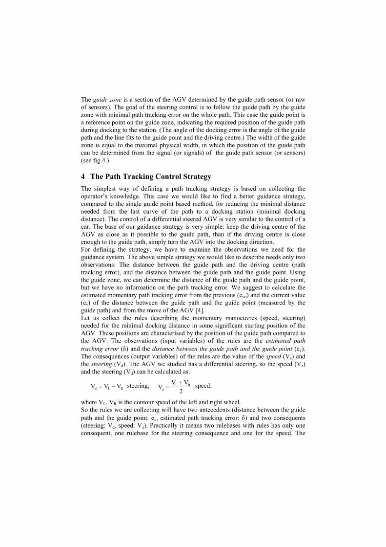
The guide zone is a section of the AGV determined by the guide path sensor (or raw of sensors). The goal of the steering control is to follow the guide path by the guide zone with minimal path tracking error on the whole path. This case the guide point is a reference point on the guide zone, indicating the required position of the guide path during docking to the station. (The angle of the docking error is the angle of the guide path and the line fits to the guide point and the driving centre.) The width of the guide zone is equal to the maximal physical width, in which the position of the guide path can be determined from the signal (or signals) of the guide path sensor (or sensors) (see fig.4.). 4 The Path Tracking Control Strategy The simplest way of defining a path tracking strategy is based on collecting the operator’s knowledge. This case we would like to find a better guidance strategy, compared to the single guide point based method, for reducing the minimal distance needed from the last curve of the path to a docking station (minimal docking distance). The control of a differential steered AGV is very similar to the control of a car. The base of our guidance strategy is very simple: keep the driving centre of the AGV as close as it possible to the guide path, than if the driving centre is close enough to the guide path, simply turn the AGV into the docking direction. For defining the strategy, we have to examine the observations we need for the guidance system. The above simple strategy we would like to describe needs only two observations: The distance between the guide path and the driving centre (path tracking error), and the distance between the guide path and the guide point. Using the guide zone, we can determine the distance of the guide path and the guide point, but we have no information on the path tracking error. We suggest to calculate the estimated momentary path tracking error from the previous (evo) and the current value (ev) of the distance between the guide path and the guide point (measured by the guide path) and from the move of the AGV [4]. Let us collect the rules describing the momentary manoeuvres (speed, steering) needed for the minimal docking distance in some significant starting position of the AGV. These positions are characterised by the position of the guide path compared to the AGV. The observations (input variables) of the rules are the estimated path tracking error (δ) and the distance between the guide path and the guide point (ev). The consequences (output variables) of the rules are the value of the speed (Va) and the steering (Vd). The AGV we studied has a differential steering, so the speed (Va) and the steering (Vd) can be calculated as:

V V Vd L R= − steering, VV V

aL R=+2

speed.

where VL, VR is the contour speed of the left and right wheel. So the rules we are collecting will have two antecedents (distance between the guide path and the guide point: ev, estimated path tracking error: δ) and two consequents (steering: Vd, speed: Va). Practically it means two rulebases with rules has only one consequent, one rulebase for the steering consequence and one for the speed. The

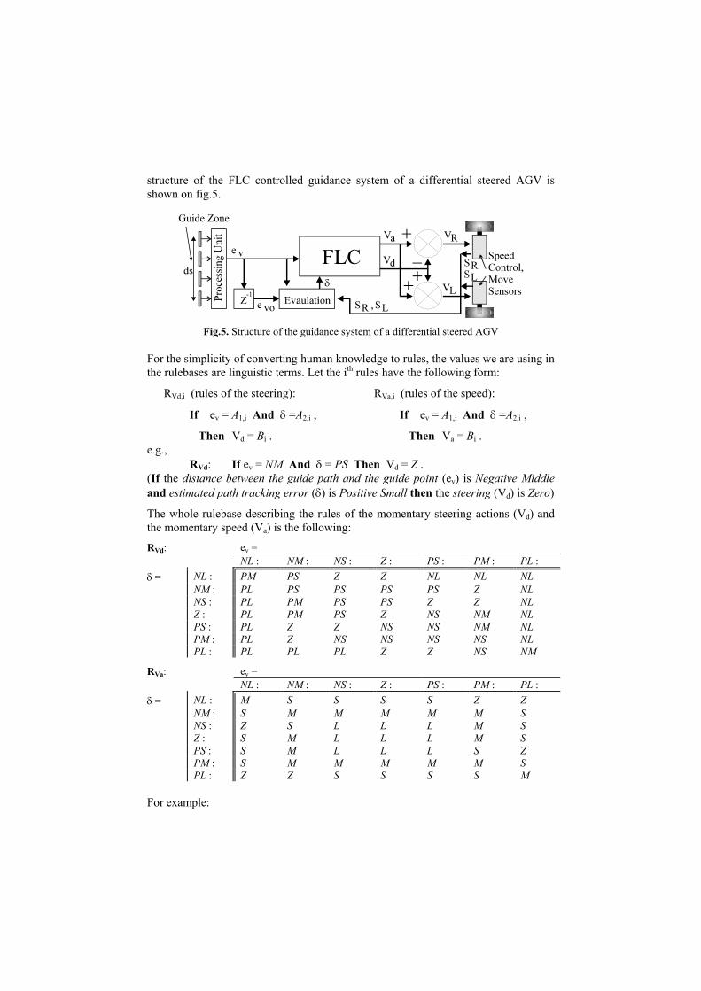
structure of the FLC controlled guidance system of a differential steered AGV is shown on fig.5.

Fig.5. Structure of the guidance system of a differential steered AGV

For the simplicity of converting human knowledge to rules, the values we are using in the rulebases are linguistic terms. Let the ith rules have the following form:

RVd,i (rules of the steering):

If ev = A1,i And δ =A2,i ,

Then Vd = Bi .

RVa,i (rules of the speed):

If ev = A1,i And δ =A2,i ,

Then Va = Bi .

e.g., RVd: If ev = NM And δ = PS Then Vd = Z . (If the distance between the guide path and the guide point (ev) is Negative Middle and estimated path tracking error (δ) is Positive Small then the steering (Vd) is Zero)

The whole rulebase describing the rules of the momentary steering actions (Vd) and the momentary speed (Va) is the following:

RVd: ev = NL : NM : NS : Z : PS : PM : PL : δ = NL : PM PS Z Z NL NL NL NM : PL PS PS PS PS Z NL NS : PL PM PS PS Z Z NL Z : PL PM PS Z NS NM NL PS : PL Z Z NS NS NM NL PM : PL Z NS NS NS NS NL PL : PL PL PL Z Z NS NM

RVa: ev = NL : NM : NS : Z : PS : PM : PL : δ = NL : M S S S S Z Z NM : S M M M M M S NS : Z S L L L M S Z : S M L L L M S PS : S M L L L S Z PM : S M M M M M S PL : Z Z S S S S M For example:

Pv

w

K

Pv

w

K

Pv

w

K

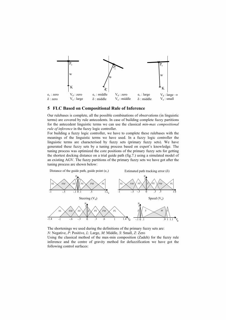
ev : zero Vd : zero ev : middle Vd : zero ev : large Vd : large → δ : zero Va : large δ : middle Va : middle δ : middle Va : small 5 FLC Based on Compositional Rule of Inference Our rulebases is complete, all the possible combinations of observations (in linguistic terms) are covered by rule antecedents. In case of building complete fuzzy partitions for the antecedent linguistic terms we can use the classical min-max compositional rule of inference in the fuzzy logic controller. For building a fuzzy logic controller, we have to complete these rulebases with the meanings of the linguistic terms we have used. In a fuzzy logic controller the linguistic terms are characterised by fuzzy sets (primary fuzzy sets). We have generated these fuzzy sets by a tuning process based on expert’s knowledge. The tuning process was optimized the core positions of the primary fuzzy sets for getting the shortest docking distance on a trial guide path (fig.7.) using a simulated model of an existing AGV. The fuzzy partitions of the primary fuzzy sets we have got after the tuning process are shown below:

Distance of the guide path, guide point (ev) Estimated path tracking error (δ) µ

Z

PMPS PLNM NSNL

1

0 .1 .5 1-.1-.5-1 ev

µ

Z PMPS PLNMNL

1

0 .3 .5 1-.3-.5-1 δ

NS

Steering (Vd) Speed (Va) µ

Z PMPS PLNM NSNL

1

0 .3 .6 1-.3-.6-1-1.4 Vd1.4

µ

Z MS L

1

0 .1 .9 1-.1 Va1.1 The shortenings we used during the definitions of the primary fuzzy sets are: N: Negative, P: Positive, L: Large, M: Middle, S: Small, Z: Zero Using the classical method of the max-min composition (Zadeh) for the fuzzy rule inference and the centre of gravity method for defuzzification we have got the following control surfaces:

-0.5

0

0.5 -1-0.5

00.5

1-1.5

-1

-0.5

0

0.5

1

1.5

ev

δ

Vd

-0.50

0.5 -1-0.5

00.5

10

0.5

1

1.5

ev

δ

Va

Fig.6. Control surface of the steering (Vd) and the speed (Va) For checking the performance of the fuzzy logic controller (FLC) based on CRI, we have worked out a simulated model for a differential steered AGV and an implementation of the FLC. Using this model we have approximated the minimal docking distance of the simulated AGV. The trial guide path we used, and the minimal docking distances in function of the guide path radius are shown on fig.7. For comparing the results of the minimal docking distances to the single guide point based steering system, its calculated results are shown on Fig.7. too.

-2 -1 0 1 2

-1

0

1

2

3

0 2 4 6 8 100

0.5

0.5

1

1.5

2

2.5

3

3.5

4

R [m]

[m]dS

1vp

FLC

Fig.7. Minimal docking distances (dS) calculated for the optimal single guide point based steering system (1vp) and the simulated results of the AGV using the CRI based FLC path

tracking strategy (FLC) in function of the trial guide path radius (R) 6 FLC Based on Interpolation in the Vague Environment For showing the efficiency of the proposed approximate fuzzy reasoning method, the size of the rulebase, describing the path tracking strategy, is reduced dramatically. All the unimportant rules, rules concluded from the other rules, are removed from the rulebase. It means, that this rulebase contains the most important rules only, so its

completeness is necessary. The reduced rulebase, describing the rules of the momentary steering actions (Vd) and the momentary speed (Va) is the following:

RVd: ev = NL : NM : Z : PM : PL : δ = NL : NL NM : PL PS PS NL Z : PL NL PM : PL NS NS NL PL : PL

RVa: ev = NL : NM : Z : PM : PL : δ = NL : Z NM : Z : S L S PM : PL : Z It is interesting to notice, that while in the rulebase of the steering (Vd) the conclusion of the rule ev:zero and δ:zero can be concluded from the surrounding rules so it has no importance at all (it is missing from the rulebase), in the rulebase of the speed (Va) this is one of the most important rules. The next step of building the fuzzy controller based on approximate fuzzy reasoning based on the vague environment of the fuzzy rulebase is to generate the vague environments of the antecedent and consequent universes. For comparing the efficiency of the proposed approximate fuzzy reasoning method in the implementation of the path tracking control strategy to the previously introduced classical CRI based fuzzy logic controller, we have applied the same simulated model and environmental parameters for tuning the vague environments (scaling functions) and the points of the linguistic variables. Similarly to the previous example, the tuning process was optimized the core positions and the scaling factor values of the linguistic terms for getting the shortest docking distance on the trial guide path (fig.9.). The vague environments (scaling functions) of the antecedent and consequent universes we have got after the tuning process are shown below:

Distance of the guide path, guide point (ev) Path tracking error (δ)

Z PM

PL

NM

NL

0 .5 1-.5-1 ev

s

1

5

10

2Z PM PLNMNL

0 .5 1-.5-1

s

1

5

10

2

δ

Steering (Vd) Speed (Va)

Vd

PS PLNSNL

0 .2 1-.2-1

s

1

5

10

2

Va

Z L

0 1

s

1

5

10

2

Applying the proposed approximate fuzzy reasoning method based on rational interpolation (introduced in point two) we have got the following control surfaces (for some kind of analogy to the center of gravity defuzzification, the sensitivity factor is chosen to two (p=2)):

-0.5

0

0.5-1 -0.5

00.5

1-1.5

-1

-0.5

0

0.5

1

1.5

ev

δ

Vd

-0.5

0

0.5 -1-0.5

00.5

10

0.5

1

1.5

ev

δ

Va

Fig.8. Control surface of the steering (Vd) and the speed (Va) (the rule points are signed by *) 7 Comparing the Simulated Results For comparing the efficiency of the simulated fuzzy logic controllers based on the classical CRI and the proposed approximate fuzzy reasoning method, during the tests we have applied the same simulated model and environmental parameters. The results, the minimal docking distances on the trial guide path in function in function of the path radius are summarized on fig.10.

Summarizing our results, on the trial guide path we have used, there are no significant differences in minimal docking distances of the two simulated implementations of the FLC (classical CRI and the proposed approximate fuzzy reasoning) path tracking strategies. In both cases these results are always better than the minimal docking distance calculated for the optimal, single guide point based steering system (fig.7,10). So using any of our path tracking guidance systems, the minimal distance needed for a possible station from the last curve of the guide path can be reduced considerably. This is the conclusion we were expected. Both rulebases, the complete (for CRI) and the sparse (for approximate reasoning) one, were fetched from the same “expert knowledge” describing the same path tracking strategy. So the simulated results of the two solutions should not be differ dramatically from each other.

The main difference is in the number of the rules required for getting similar results. In spite of the radical reduction of the number of the fuzzy rules, there are no notable differences in the efficiency of the two solutions. (In case of the rulebase of the steering the complete rulebase contains 49 rules, while the sparse rulebase (used by the approximate reasoning method) contains only 12 rules, in case of the rulebase of the speed the reduction is from 49 to 5.) In other words it means, that using the concept of vague environment in most of the practical cases we can build approximate fuzzy reasoning methods simple enough to be a good alternative of the classical Compositional Rule of Inference methods in practical applications.

-2 -1 0 1 2

-1

0

1

2

3

.5.3 R [m]

[m]dS

FLC

FLC

approx.

0 2 4 6 8 100

0.2

0.4

0.6

0.8

1

1.2

Fig.9. Simulated results of the AGV

using the approximate fuzzy reasoning based

FLC path tracking strategy

Fig.10. Simulated results of the minimal docking distances (dS) using the CRI based FLC (FLC)

and the approximate fuzzy reasoning based (FLCapprox.) path tracking strategy

in function of the trial guide path radius (R)

References 1. Klawonn, F.: Fuzzy Sets and Vague Environments, Fuzzy Sets and Systems, 66,

pp207-221, (1994). 2. Kovács, Sz., Kóczy, L.T.: Fuzzy Rule Interpolation in Vague Environment,

Proceedings of the 3rd. European Congress on Intelligent Techniques and Soft Computing, pp.95-98, Aachen, Germany, (1995).

3. Kovács, Sz.: New Aspects of Interpolative Reasoning, Proceedings of the 6th. International Conference on Information Processing and Management of Uncertainty in Knowledge-Based Systems, pp.477-482, Granada, Spain, (1996).

4. Cselényi, J., Kovács, Sz., Pap, L., Kóczy, L.T.: New concepts in the fuzzy logic controlled path tracking strategy of the differential steered AGVs, Proceedings of the 5th International Workshop on Robotics in Alpe-Adria-Danube Region, p.6, Budapest, Hungary, (1996).

5. Hammond, G.: AGVS at Work - Automated Guided Vehicle Systems. Springer-Verlag, p.232., (1986).