application of support vector machines in bioinformatics
TRANSCRIPT

Application of Support Vector Machinesin Bioinformatics
by
Jung-Ying Wang
A dissertation submitted in partial fulfillmentof the requirements for the degree of
Master of Science(Computer Science and Information Engineering)
in National Taiwan University2002
c© Jung-Ying Wang 2002All Rights Reserved

ABSTRACT
Recently a new learning method called support vector machines (SVM) has showncomparable or better results than neural networks on some applications. In this thesiswe exploit the possibility of using SVM for three important issues of bioinformatics:the prediction of protein secondary structure, multi-class protein fold recognition,and the prediction of human signal peptide cleavage sites. By using similar data,we demonstrate that SVM can easily achieve comparable accuracy as using neuralnetworks. Therefore, in the future it is a promising direction to apply SVM on morebioinformatics applications.
ii

ACKNOWLEDGEMENTS
I would like to thank Chih-Jen Lin, my advisor, for his many suggestions and
constant support during my research.
To my family I give my appreciation for their support and love over the years.
Without them this work would have never come into existence.
Taipei 106, Taiwan Jung-Ying Wang
December 3, 2001
iii

TABLE OF CONTENTS
ABSTRACT . . . . . . . . . . . . . . . . . . . . . . . . . . . . . . . . . . . ii
ACKNOWLEDGEMENTS . . . . . . . . . . . . . . . . . . . . . . . . . . iii
LIST OF TABLES . . . . . . . . . . . . . . . . . . . . . . . . . . . . . . . . vi
LIST OF FIGURES . . . . . . . . . . . . . . . . . . . . . . . . . . . . . . . viii
CHAPTER
I. Introduction . . . . . . . . . . . . . . . . . . . . . . . . . . . . . . 1
1.1 Background . . . . . . . . . . . . . . . . . . . . . . . . . . . . 11.2 Protein Secondary Structure Prediction . . . . . . . . . . . . 21.3 Protein Fold Prediction . . . . . . . . . . . . . . . . . . . . . 31.4 Signal Peptide Cleavage Sites . . . . . . . . . . . . . . . . . . 6
II. Support Vector Machines . . . . . . . . . . . . . . . . . . . . . . 8
2.1 Basic Concepts of SVM . . . . . . . . . . . . . . . . . . . . . 82.2 For Multi-class SVM . . . . . . . . . . . . . . . . . . . . . . . 12
2.2.1 One-against-all Method . . . . . . . . . . . . . . . . 122.2.2 One-against-one Method . . . . . . . . . . . . . . . 13
2.3 Software and Model Selection . . . . . . . . . . . . . . . . . . 13
III. Protein Secondary Structure Prediction . . . . . . . . . . . . . 15
3.1 The Goal of Secondary Structure Prediction . . . . . . . . . . 153.2 Data Set Used in Protein Secondary Structure . . . . . . . . 153.3 Coding Scheme . . . . . . . . . . . . . . . . . . . . . . . . . . 163.4 Assessment of Prediction Accuracy . . . . . . . . . . . . . . . 17
IV. Protein Fold Recognition . . . . . . . . . . . . . . . . . . . . . . 21
4.1 The Goal of Protein Fold Recognition . . . . . . . . . . . . . 214.2 Data Set and Feature Vectors . . . . . . . . . . . . . . . . . . 21
iv

4.3 Multi-class Methodologies for Protein Fold Classification . . . 224.4 Measure for Protein Fold Recognition . . . . . . . . . . . . . 26
V. Prediction of Human Signal Peptide Cleavage Sites . . . . . . 29
5.1 The Goal of Predicting Signal Peptide Cleavage Sites . . . . . 295.2 Coding Schemes and Feature Vector Extraction . . . . . . . . 295.3 Using SVM to Combine Cleavage Sites Predictors . . . . . . . 325.4 Measures of Cleavage Sites Prediction Accuracy . . . . . . . . 33
VI. Results . . . . . . . . . . . . . . . . . . . . . . . . . . . . . . . . . . 34
6.1 Comparison of Protein Second Structure Prediction . . . . . . 346.2 Comparison of Protein Fold Recognition . . . . . . . . . . . . 366.3 Comparison of Signal Peptide Cleavage Sites Prediction . . . 41
VII. Conclusions and Discussions . . . . . . . . . . . . . . . . . . . . 43
7.1 Protein Secondary Structure Prediction . . . . . . . . . . . . 437.2 Multi-class Protein Fold Recognition . . . . . . . . . . . . . . 447.3 Signal Peptide Cleavage Sites Prediction . . . . . . . . . . . . 44
APPENDICES . . . . . . . . . . . . . . . . . . . . . . . . . . . . . . . . . . 45
BIBLIOGRAPHY . . . . . . . . . . . . . . . . . . . . . . . . . . . . . . . . 51
v

LIST OF TABLES
Table
3.1 130 protein chains used for seven-fold cross validation. . . . . . . . . 18
4.1 Non-redundant subset of 27 SCOP folds using in training and testing 23
4.2 Six parameter sets extracted from protein sequence . . . . . . . . . 23
4.3 Prediction accuracy Qi in percentage using high confidence only . . 27
5.1 Properties of amino acid residues . . . . . . . . . . . . . . . . . . . 31
5.2 Relative hydrophobicity of amino acids . . . . . . . . . . . . . . . . 32
6.1 SVM for protein secondary structure prediction. Using the seven-fold cross validation on RS130 protein set . . . . . . . . . . . . . . . 35
6.2 SVM for protein secondary structure prediction. Using the quadraticpenalty term and the seven-fold cross validation on RS130 protein set 35
6.3 Prediction accuracy Qi for protein fold in percentage for the inde-pendent test set . . . . . . . . . . . . . . . . . . . . . . . . . . . . . 37
6.4 (Cont’d) Prediction accuracy Qi for protein fold in percentage forthe independent test set . . . . . . . . . . . . . . . . . . . . . . . . 38
6.5 Prediction accuracy Qi for protein fold in percentage for the ten-foldcross validation. . . . . . . . . . . . . . . . . . . . . . . . . . . . . . 39
6.6 The best parameters C and γ chosen for each subsystem and thecombiner . . . . . . . . . . . . . . . . . . . . . . . . . . . . . . . . . 41
6.7 Comparison of SVM with ACN and SignalP methods . . . . . . . . 42
A.1 Optimal hyperparameters for the training set by 10-fold cross vali-dation. . . . . . . . . . . . . . . . . . . . . . . . . . . . . . . . . . . 47
vi

A.2 (Cont’d) Optimal hyperparameters for the training set by 10-foldcross validation. . . . . . . . . . . . . . . . . . . . . . . . . . . . . . 48
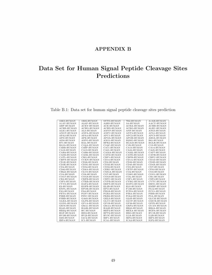
B.1 Data set for human signal peptide cleavage sites prediction . . . . . 49
B.2 (Cont’d) Data set for human signal peptide cleavage sites prediction 50
vii

LIST OF FIGURES
Figure
1.1 Region of SCOP hierarchy . . . . . . . . . . . . . . . . . . . . . . . 5
2.1 Separating hyperplane . . . . . . . . . . . . . . . . . . . . . . . . . 10
2.2 An example which is not linear separable . . . . . . . . . . . . . . . 10
3.1 An example of using evolutionary information to coding secondarystructure . . . . . . . . . . . . . . . . . . . . . . . . . . . . . . . . . 19
4.1 Predictor for multi-class protein fold recognition . . . . . . . . . . . 27
6.1 A comparison of 27 folds for independent test set . . . . . . . . . . 40
6.2 A comparison of 27 folds for ten-fold cross validation . . . . . . . . 40
viii

CHAPTER I
Introduction
1.1 Background
Bioinformatics is an emerging and rapidly growing field of science. As a conse-
quence of the large amount of data produced in the field of molecular biology, most
of the current bioinformatics projects deal with structural and functional aspects of
genes and proteins. The data produced by thousands of research teams all over the
world are collected and organized in databases specialized for particular subjects.
The existence of public databases with billions of data entries requires a robust
analytical approach to cataloging and representing this with respect to its biological
significance. Therefore, computational tools are needed to analyze the collected data
in the most efficient manner. For example, working on the prediction of the biological
functions of genes and proteins (or parts of them) based on structural data.
Recently support vector machines (SVM) has been a new and promising tech-
nique for machine learning. On some applications it has obtained higher accuracy
than neural networks (for example, [17]). SVM has also been applied to biological
problems. Some examples are [6, 80]. In this thesis we exploit the possibility of using
SVM for three important issues of bioinformatics: the prediction of protein secondary
structure, multi-class protein fold recognition, and the prediction of human signal
1

peptide cleavage sites.
1.2 Protein Secondary Structure Prediction
Recently prediction for the structure and function of proteins has become in-
creasingly important. A step on the way to obtain the full three-dimensional (3D)
structure is to predict the local conformation of the polypeptide chain, which is called
the secondary structure. The secondary structure consists of local folding regulari-
ties maintained by hydrogen bonds and is traditionally subdivided into three classes:
alpha-helices, beta-sheets, and coil.
The sequence preferences and correlations involved in these structures have made
secondary structure one of the classical problems in computational molecular biology,
and one where machine learning approaches have been particularly successful. See
[1] for a detailed review.
Many pattern recognition and machine learning methods have been proposed to
solve this issue. Surveys are, for example, [63, 66]. Some typical approaches are as
follows: (i) statistical information [49, 61, 53, 25, 28, 3, 26, 45, 78, 36, 19] ; (ii)
physico-chemical properties [59] ; (iii) sequence patterns [75, 12, 62] ; (iv) multi-
layered (or neural) networks [4, 60, 30, 40, 74, 83, 64, 65, 46, 9] ; (v) graph-theory
[50, 27] ; (vi) multivariate statistics [38] ; (vii) expert rules [51, 24, 27, 84] ; and
(viii) nearest-neighbor algorithms [82, 72, 68].
Among these machine learning methods, neural networks may be the most pop-
ular and effective one for the secondary structure prediction. Up to now the highest
accuracy is achieved by approaches using it. In 1988, secondary structure prediction
directly using Neural Networks first achieved about 62% accuracy [60, 30]. In 1993,
using evolutionary information, a Neural Network system had improved the predic-
2

tion accuracy to over 70% [65]. Recently there have been approaches (e.g. [58, 1])
using neural networks which achieve even higher accuracy (> 75%).
In this thesis, we apply SVM for protein secondary structure prediction. We
worked on similar data and encoding schemes as those in Rost and Sander [65]
(referred here as RS130). The performance accuracy is verified by a seven-fold cross
validation.
Results indicate that SVM easily returns comparable results as neural networks.
Therefore, in the future it is a promising direction to study other applications by
using SVM.
1.3 Protein Fold Prediction
A key to understand the function of biological macromolecules, e.g., proteins,
is the determination of the three-dimensional (3D) structure. Large-scale gene-
sequencing projects accumulate a massive number of putative protein sequences.
However, information about 3D structures is available for only a small fraction of
known proteins. Thus, although experimental structure determination has improved,
the sequence-structure gap continues to increase.
This creates a need for extracting structural information from sequence databases.
The direct prediction of a protein’s 3D structure from a sequence remains elusive.
However, considerable progress has been shown in assigning a sequence to a fold class.
There have been two general approaches to this problem. One is to use threading
algorithms. The other is a taxonometric approach which presumes that the number
of folds is restricted and thus the focus is on structural predictions in the context of
a particular classification of 3D folds. Proteins are defined as having a common fold
if they have the same major secondary structures in the same arrangement and with
3

the same topological connections. To facilitate access to this information, Hubbard
et al. [32] constructed the Structural Classification of Proteins (SCOP) database.
The SCOP database is a publicly accessible database over the internet. It stores
a set of protein sequences which have been hand-classified into a hierarchical struc-
ture based on their structure and function. The SCOP database aims to provide
a detailed and comprehensive description of the structural and evolutionary rela-
tionships between all proteins whose structure is known, including all entries in the
Protein Data Bank (PDB). The distinction between evolutionary relationships and
those that arise from the physics and chemistry of proteins is a feature that is unique
to this database. The database is freely accessible on the web with an entry point
at URL http : //scop.mrc− lmb.cam.ac.uk/scop/.
Many levels exist in the SCOP hierarchy, which are illustrated in Figure 1.1 [32].
The principal levels are family, superfamily, and fold, which will be described below.
Family: Homology is a clear indication of shared structures and frequently related
functions. At the simplest level of similarity we can group proteins into families of
homologus sequences with a clear evolutionary relationship.
Superfamily: Superfamilies can be loosely defined as composition of families with
a probable evolutionary relationship, supported mainly by common structural and
functional features, in the absence of detectable sequence homology.
Fold: Folds can be described as representing the architecture of proteins. Two
proteins will have a common fold if they have comparable elements of secondary
structure with the same topology of connections.
4

� � � �
� � � � �
� � � �
� � � � � � � �
� � � � � �
� � � � � �
� � �
α β
� � � � � � � � � � � � � � � � � � � � � � � � � � �
� � � � � � � � � � � � � � � � �
β � � � � � � � � � � � � � ! " # β � � � � � � �
$ � � �
% � � α � � � � � � � �
& � � � $ � � �
� � � � � � � � � � � �
' � ( ' ( � ' (
� � � � � � � � � � � � � � �
α � % � � � � � � ! ) # β � % � � � � � �
� � � � � � � � � � � � � � � � � � � � � � ! � #
α+β � � � �
α/β α+β
� * �
Figure 1.1: Region of SCOP hierarchy
In this thesis a computational method based on SVM has been developed for the
assignment of a protein sequence to a folding class in the SCOP. We investigated
two strategies for multi-class SVM: “one-against-all” and “one-against-one”. Then
we combine these two methods with a voting process to do the classification of 27
folds of data. Comparing to general classification problem this data set has very few
data. Applying our method increases the overall prediction accuracy to 63.6% when
using an independent test set and 52.7% when using the ten-fold cross validation on
the training set. Both improve the current prediction accuracy by more than 7%.
The experimental results reveal that model selection is an important step in SVM
design.
5

1.4 Signal Peptide Cleavage Sites
Signal peptides target proteins for secretion in both prokaryotic and eukaryotic
cells. The signal peptide of the nascent protein on a free ribosome is recognized by
Signal Recognition Particle (SRP) which arrests translation. SRP then binds an SRP
receptor on the endoplasmic reticulum (ER) membrane and inserts the signal peptide
into the membrane. Translation resumes, and the protein is translocated through
the membrane into the ER lumen as it is synthesized. Other sequence determinants
on the protein then dictate whether it will remain in the ER lumen, or pass on to
one of the other membrane-bound compartments, or be secreted from the cell.
Signal peptides control the entry of virtually all proteins to the secretory pathway.
They comprise the N -terminal part of the amino acid chain, and are cleaved off
while the protein is translocated through the membrane. The common structure of
signal peptides consist of three regions: a positively charged n-region, followed by
a hydrophobic h-region, and a neutral but polar c-region [79]. The cleavage site is
generally characterized by neutral small side-chain amino acids at positions -1 and
-3 (relative to the cleavage site) [55, 56].
Strong interest in prediction of the signal peptides and their cleavage sites has
been evoked not only by the huge amount of unprocessed data available, but also
by the industrial need to find more effective vehicles for production of proteins in
recombinant systems.
In this thesis, we use four independent SVM coding schemes (“subsystems”) to
learn the mapping between amino acid sequences and signal peptide cleavage sites
from the known protein structures and physico-chemical properties. Then a SVM
combiner learns to combine the outputs of the four subsystems to make final predic-
6

tions. To have a fair comparison, we consider similar data and the same encoding
scheme used in ACN [33] for negative patterns, and compared with two established
predictors (SignalP ([55, 56]) and ACN) for signal peptides. We demonstrate that
SVM can achieve higher accuracy then using SignalP and ACN.
7

CHAPTER II
Support Vector Machines
2.1 Basic Concepts of SVM
The support vector machine (SVM) is a new and promising technique for data
classification and regression. After the development in the past five years, it has
become an important topic in machine learning and pattern recognition. Not only it
has a better theoretical foundation, practical comparisons have also shown that it is
competitive with existing methods such as neural networks and decision trees (e.g.
[43, 7, 17]).
Existing surveys and books on SVM are, for example, [14, 76, 77, 8, 71, 15].
The number of applications of SVM is dramatically increasing, for example, object
recognition [57], combustion engine detection [67], function estimation [73], text cat-
egorization [34], chaotic system [52], handwritten digit recognition [47], and database
marketing [2].
The SVM technique was first developed by Vapnik and his group in former AT&T
Bell Laboratories. The original idea is to use a linear separating hyperplane which
maximizes the distance between two classes to create a classifier. For problems which
can not be linearly separated in the original input space, support vector machines
employ two techniques to deal this case. First we introduce a soft margin hyperplane
8

which adds a penalty function of violation of constraints to our optimization criterion.
Secondly we non-linearly transform the original input space into a higher dimension
feature space. Then in this new feature space it is more possible to find a linear
optimal separating hyperplane.
Given training vectors xi, i = 1, . . . , l of length n, and a vector y defined as follows
yi =
1 if xi in class 1,
−1 if xi in class 2,
The support vector technique tries to find the separating hyperplane with the largest
margin between two classes, measured along a line perpendicular to the hyperplane.
For example, in Figure 2.1, two classes could be fully separated by a dotted line
wT x + b = 0. We would like to decide the line with the largest margin. In other
words, intuitively we think that the distance between two classes of training data
should be as large as possible. That means we want to find a line with parameters w
and b such that the distance between wT x + b = ±1 is maximized. As the distance
between wT x + b = ±1 is 2/‖w‖ and maximizing 2/‖w‖ is equivalent to minimizing
wT w/2, we have the following problem:
minw,b
12wT w
yi((wT xi) + b) ≥ 1, (2.1)
i = 1, . . . , l.
The constraint yi((wT xi) + b) ≥ 1 means
(wT xi) + b ≥ 1 if yi = 1,
(wT xi) + b ≤ −1 if yi = −1.
That is, data in the class 1 must be on the right-hand side of wT x+b = 0 while data in
the other class must be on the left-hand side. Note that the reason of maximizing the
9
wT x + b =
+10−1
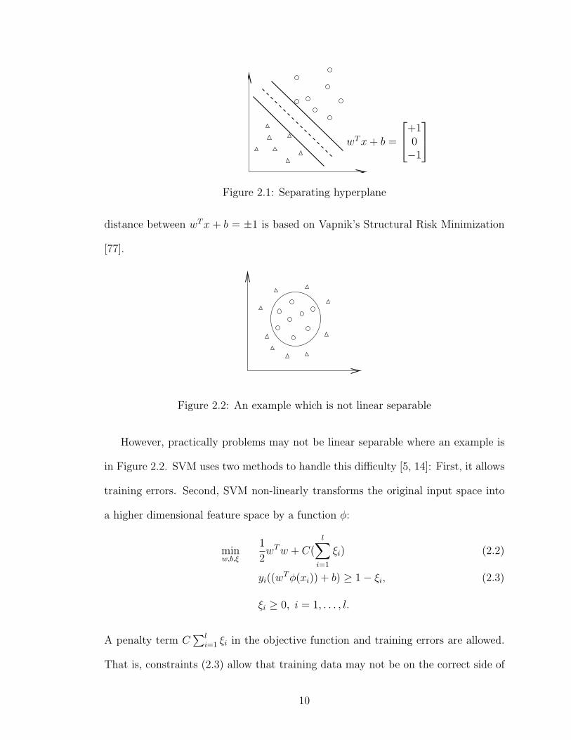
Figure 2.1: Separating hyperplane
distance between wT x + b = ±1 is based on Vapnik’s Structural Risk Minimization
[77].
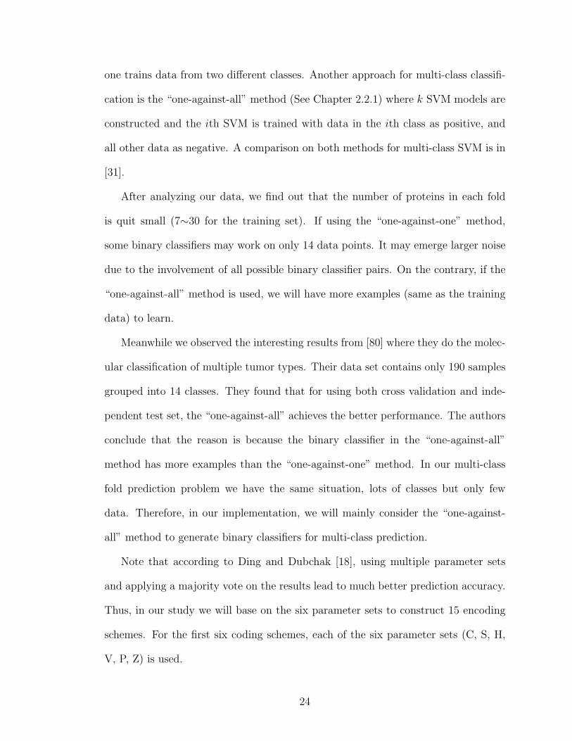
Figure 2.2: An example which is not linear separable
However, practically problems may not be linear separable where an example is
in Figure 2.2. SVM uses two methods to handle this difficulty [5, 14]: First, it allows
training errors. Second, SVM non-linearly transforms the original input space into
a higher dimensional feature space by a function φ:
minw,b,ξ
12wT w + C(
l∑
i=1
ξi) (2.2)
yi((wT φ(xi)) + b) ≥ 1− ξi, (2.3)
ξi ≥ 0, i = 1, . . . , l.
A penalty term C∑l
i=1 ξi in the objective function and training errors are allowed.
That is, constraints (2.3) allow that training data may not be on the correct side of
10

the separating hyperplane wT x + b = 0 while we minimize the training error∑l
i=1 ξi
in the objective function. Hence if the penalty parameter C is large enough and
the data is linear separable, problem (2.3) goes back to (2.1) as all ξi will be zero
[44]. Note that training data x is mapped into a (possibly infinite) vector in a higher
dimensional space:
φ(x) = (φ1(x), φ2(x), . . .).
In this higher dimensional space, it is more possible that data can be linearly sepa-
rated. An example by mapping x from R3 to R10 is as follows:
φ(x) = (1,√
2x1,√
2x2,√
2x3, x21, x
22, x
23,√
2x1x2,√
2x1x3,√
2x2x3),
Hence (2.2) is a problem in an infinite dimensional space which is not easy. Cur-
rently the main procedure is by solving a dual formulation of (2.2). It needs a closed
form of K(xi, xj) ≡ φ(xi)T φ(xj) which is usually called the kernel function. Some
popular kernels are, for example, RBF kernel: e−γ‖xi−xj‖2 and polynomial kernel:
(xTi xj/γ + δ)d, where γ and δ are parameters.
After the dual form is solved, the decision function is written as
f(x) = sign(wT φ(x) + b).
In other words, for a test vector x, if wT φ(x) + b > 0, we classify it to be in the class
1. Otherwise, we think it is in the second class. Only some of xi, i = 1, . . . , l are
used to construct w and b and they are important data called support vectors. In
general, the number of support vectors is not large. Therefore we can say SVM is
used to find important data (support vectors) from training data.
11

2.2 For Multi-class SVM
2.2.1 One-against-all Method
The earliest used implementation for SVM multi-class classification is probably
the one-against-all method. It constructs k SVM models where k is the number
of classes. The ith SVM is trained with all of the examples in the ith class with
positive labels, and all other examples with negative labels. Thus given l training
data (x1, y1), . . . , (xl, yl), where xi ∈ Rn, i = 1, . . . , l and yi ∈ {1, . . . , k} is the class
of xi, the ith SVM is by solving the following problem:
minwi,bi,ξi
12(wi)T wi + C
l∑
j=1
(ξi)j
(wi)T φ(xj)) + bi ≥ 1− ξij, if yj = i, (2.4)
(wi)T φ(xj)) + bi ≤ −1 + ξij, if yj 6= i,
ξij ≥ 0, j = 1, . . . , l,
where training data xi are mapped to a higher dimensional space by the function φ
and C is the penalty parameter. Then there are k decision functions:
(w1)T φ(x) + b1,
...
(wk)T φ(x) + bk.
Generally, we say x is in the class which has the largest value of the decision function:
class of x = argmaxi=1,...,k((wi)T φ(x) + bi).
In this thesis we will use another strategy. On the SCOP database with 27 folds,
we build 27 “one-against-all” classifiers. Each protein in the test set is tested against
all 27 “one-against-all” classifiers. If the result is “positive”, then we will assign a
12

vote for the class. However, if the result is “negative”, representation the protein
belongs to one of the 26 other folds. In other words, the protein belongs to each of
the other 26 folds with a probability of 1/26. Therefore, in our coding we do not
assign any vote to this case.
2.2.2 One-against-one Method
Another major method is called the one-against-one method. It was first in-
troduced in [41], and the first use of this strategy on SVM was in [23, 42]. This
method constructs k(k−1)/2 classifiers where each one trains data from two classes.
For training data from the ith and the jth classes, we solve the following binary
classification problem:
minwij ,bij ,ξij
12(wij)T wij + C(
∑
t
(ξij)t)
((wij)T φ(xt)) + bij) ≥ 1− ξijt , if yt = i, (2.5)
((wij)T φ(xt)) + bij) ≤ −1 + ξijt , if yt = j,
ξijt ≥ 0.
There are different methods for doing the future testing after all k(k−1)/2 classifiers
are constructed. In this thesis, we use the following voting strategy suggested in [23]:
if sign((wij)T φ(x) + bij)) says x is in the ith class, then the vote for the ith class is
added by one. Otherwise, the jth is increased by one. Then we predict x is in the
class with the largest vote. The voting approach described above is also called the
“Max Wins” strategy.
2.3 Software and Model Selection
We use the software LIBSVM [10] for experiments. LIBSVM is a general li-
brary for support vector classification and regression, which is available at http :
13

//www.csie.ntu.edu.tw/~cjlin/libsvm.
As mentioned in Section 2.1 that there are different functions φ to map data to
higher dimensional spaces, practically we need to select the kernel function K(xi, xj) =
φ(xi)T φ(xj). There are several types of kernels in used with all kinds of problems.
Each kernel may be more suitable for some problems. For example, some well-known
problems with large amount of features, such as text classification [35] and DNA prob-
lems [81], are reported to be classified more correctly with the linear kernel. In our
experience, the RBF kernel is a decent choice for most problems. A learner with the
RBF kernel usually performs no worse than others do, in terms of the generalization
ability.
In this thesis, we did some simple comparisons and observed that using the RBF
kernel the performance is a little better than the linear kernel K(xi, xj) = xTi xj for
all the problems we studied. Therefore, for the three data sets in stead of staying in
the original space a non-linear mapping to a higher dimensional space seems useful.
We then use the RBF kernel for all the experiments.
Another important issue is the selection of parameters. For SVM training, few
parameters such as the penalty parameter C and the kernel parameter γ of the
RBF function must be determined in advance. Choosing optimal parameters for
support vector machines is an important step in SVM design. From the results of
[20] we know, for the formulation (2.2), cross validation may be a better estimator
than others. So we use the cross validation on different parameters for the model
selection.
14

CHAPTER III
Protein Secondary Structure Prediction
3.1 The Goal of Secondary Structure Prediction
Given an amino acid sequence the goal of secondary structure prediction is to
predict a secondary structure state (α, β, coil) for each residue in the sequence.
Many different methods have been applied to tackle this problem. A good predictor
must be based on knowledge learned from existing data. That is, we have to train
a model using several sequences with known secondary structures. In this chapter
we will show that by a simple use of SVM, it can easily achieve as good accuracy as
using neural networks.
3.2 Data Set Used in Protein Secondary Structure
The choice of protein database for secondary structure prediction is complicated
by potential homology between proteins in the training and testing set. Homologous
proteins in the database can give misleading results since learning methods in some
cases can memorize the training set. Therefore protein chains without significant
pairwise homology are used for developing our prediction task. To have a fair com-
parison, we consider the same 130 protein sequences used in Rost and Sander [65]
for training and testing. These proteins, taken from the HSSP (Homology-derived
15

Structures and Sequence alignments of Proteins) database [69], all have less than
25% pairwise similarity and more than 80 residues. Table 3.1 lists the 130 protein
chains used in our study.
The secondary structure assignment was done according to the DSSP (Dictio-
nary of Secondary Structures of Proteins) algorithm [37], which distinguishes eight
secondary structure classes. We converted the eight types into three classes in the
following way: H (α-helix), I (π-helix), and G (310-helix) as helix (α), E (extended
strand) as β-strand (β), and all others as coil (c). Note that different conversion
methods influence the prediction accuracy to some extent, as discussed by Cuff and
Barton [16].
3.3 Coding Scheme
Before the work by Rost and Sander [65] one common coding for the secondary
structure prediction (e.g. [60, 30]) is considering a moving window of n (typically
13-21) neighboring residues and each position of a window has 21 possible values (20
amino acids and a null input). Hence the presentation of each residue can be by an
integer ranging from 1 to 21 or by 21 binary (i.e. value 0 or 1) indicators. If we take
the later approach then among the 21 binary indicators only one has the value one.
Therefore, the number of data points is the same as the number of residues while
each data point has 21× n values. These encoding methods with three-state neural
networks obtained about 63% accuracy.
A breakthrough on the encoding method is by using the evolutionary information
[65]. We use this method in our study. The key idea is for any training sequence;
we consider its related sequences as well. These related sequences provide structural
information, which is not affected by the local change of the amino acids. Instead
16

of just feeding the base sequence they feed the multiple alignment in the form of a
profile. An alignment means aligning the protein sequences so that large chunks of
the amino acid sequence align with each other. Basically the coding scheme considers
a moving window of 17 (typically 13-21) neighboring residues. For each residue the
frequency of occurrence of each 20 amino acids at one position in the alignment is
computed. In our study, the alignments (profile) are taken from the HSSP database.
The window is shifted residue by residue through the protein chain, thus yielding N
data points for a chain with N residues.
Figure 3.1 is an example of using evolutionary information for encoding where we
have aligned four proteins. In the gray column the based sequence has the residue
“K” while the multiple alignments in this position are “P”, “G”, “G” and “.” (in-
dicate point of deletion in this sequence). Finally, the frequencies are directly used
as the values of output coding. Therefore, the coding scheme in this position will be
given as G = 0.50, P = 0.25, K = 0.25.
Prediction is made for the central residue in the windows. In order to allow the
moving window to overlap the amino- or carboxyl-terminal end of the protein a null
input was added for each residue. Therefore, each data point contains 21× 17 = 357
values. Hence each data can be represented as a vector.
Note that the RS130 data set consists of 24,387 data points in three classes where
47% are coil , 32% are helix, and 21% are strand.
3.4 Assessment of Prediction Accuracy
An important fact about prediction problems is that training errors are not impor-
tant; only test errors (i.e. accuracy for predicting new sequences) count. Therefore,
it is important to estimate the generalized performance of a learning method.
17

Table 3.1: 130 protein chains used for seven-fold cross validation.
256b A 2aat 8abp 6acn 1acx 8adh 3aitset A 2ak3 A 2alp 9api A 9api B 1azu 1cyo 1bbp A
1bds 1bmv 1 1bmv 2 3blm 4bp22cab 7cat A 1cbh 1cc5 2ccy A 1cdh 1cdt A
set B 3cla 3cln 4cms 4cpa I 6cpa 6cpp 4cpv1crn 1cse I 6cts 2cyp 5cyt R1eca 6dfr 3ebx 5er2 E 1etu 1fc2 C 1fdl H
set C 1dur 1fkf 1fnd 2fxb 1fxi A 2fox 1g6n A2gbp 1a45 1gd1 O 2gls A 2gn51gpl A 4gr1 1hip 6hir 3hmg A 3hmg B 2hmz A
set D 5hvp A 2i1b 3icb 7icd 1il8 A 9ins B 1l581lap 5ldh 1gdj 2lhb 1lmb 32ltn A 2ltn B 5lyz 1mcp L 2mev 4 2or1 L 1ovo A
set E 1paz 9pap 2pcy 4pfk 3pgm 2phh 1pyp1r09 2 2pab A 2mhu 1mrt 1ppt1rbp 1rhd 4rhv 1 4rhv 3 4rhv 4 3rnt 7rsa
set F 2rsp A 4rxn 1s01 3sdh A 4sgb I 1sh1 2sns2sod B 2stv 2tgp I 1tgs I 3tim A6tmn E 2tmv P 1tnf A 4ts1 A 1ubq 2utg A 9wga A
set G 2wrp R 1bks A 1bks B 4xia A 2tsc A 1prc C 1prc H1prc L 1prc M
The database of non-homologous proteins used for seven-fold cross validation. Allproteins have less than 25% pairwise similarity for lengths great than 80 residues.
18

SH3 N S T N K D W W K sequence
to
process
index a1 N K S N P D W W E
a2 E E H . G E W W K multiple
a3 R S T . G D W W L alignment
a4 F S . . . . F F G
1 V 0 0 0 0 0 0 0 0 0
2 L 0 0 0 0 0 0 0 0 20 numeric
3 I 0 0 0 0 0 0 0 0 0 profile
4 M 0 0 0 0 0 0 0 0 0
5 F 20 0 0 0 0 0 20 20 0
6 W 0 0 0 0 0 0 80 80 0
7 Y 0 0 0 0 0 0 0 0 0
8 G 0 0 0 0 50 0 0 0 20
9 A 0 0 0 0 0 0 0 0 0
10 P 0 0 0 0 25 0 0 0 0
11 S 0 60 25 0 0 0 0 0 0
12 T 0 0 50 0 0 0 0 0 0
13 C 0 0 0 0 0 0 0 0 0
14 H 0 0 25 0 0 0 0 0 0
15 R 20 0 0 0 0 0 0 0 0
16 K 0 20 0 0 25 0 0 0 40
17 Q 0 0 0 0 0 0 0 0 0
18 E 20 20 0 0 0 25 0 0 20
19 N 40 0 0 100 0 0 0 0 0
20 D 0 0 0 0 0 75 0 0 0
Coding output: G=0.50, P=0.25, K=0.25
Figure 3.1: An example of using evolutionary information to coding secondary struc-ture
19

Several different measures for assessment the accuracy have been suggested in
the literature. The most common measure for the secondary structure prediction is
the overall three-state accuracy (Q3). It is defined as the ratio of correctly predicted
residues to the total number of residues in the database under consideration [60, 64].
Q3 is calculated by:
Q3 =qα + qβ + qcoil
N× 100, (3.1)
where N is the total number of residues in the test data sets, and qs is the number
of residues of secondary structure type s that are predicted correctly.
20

CHAPTER IV
Protein Fold Recognition
4.1 The Goal of Protein Fold Recognition
Since protein sequence information grows significantly faster than information on
protein 3D structure, the need for predicting the folding pattern of a given protein
sequence naturally arises. In this chapter a computational method based on SVM
has been developed for the assignment of a protein sequence to a folding class in the
SCOP. We investigated two strategies for multi-class SVM: “one-against-all” and
“one-against-one”. Then we combine these two methods with a voting process to do
the classification of 27 folds of data.
4.2 Data Set and Feature Vectors
Because tests based on different protein sets are hard to compare, to have a fair
comparison, we consider the same data set used in Ding and Dubchak [18, 21, 22]
for training and testing. The data set is available at http : //www.nersc.gov/ ∼
cding/protein. The training set contains 313 proteins grouped into 27 folds, which
were selected from the database built by Dubchak [22] as shown in Table 4.1. Note
that the original database is separated to form 128 folds. These proteins are subset
of the PDB-select sets [29], where two proteins have no more than 35% of sequence
21

identity for any aligned subsequences longer than 80 residues.
The independent test set contains 385 proteins in the same 27 folds. It is a
subset of PDB-40D set developed by the authors of the SCOP database [13], where
sequences having less than 40% identity are chosen. In addition, all proteins in the
PDB-40D that had more than 35% identity with proteins of the training set were
excluded from the testing set.
Here for data coding we use the same six parameter sets as Ding and Dubchak
[18]. Note that the six parameter sets, as listed in Table 4.2, were extracted from
protein sequence independently (for details see Dubchak et al. [22]) . Thus, one may
apply learning methods based on a single parameter set for protein fold prediction.
Therefore, in our coding schemes we will use each of the parameter set individual
and their combination as our input coding.
For example, the parameter set “C” considers that each protein is associated
with the percentage composition of the 20 amino acids. Therefore, the number of
data points is the same as the number of proteins where each data point has 20
dimensions (values). We can also combine two parameter sets into one dataset. For
example we can combine “C” and “H” into one dataset “CH”, so each data point
has 20 + 21 = 41 dimensions.
4.3 Multi-class Methodologies for Protein Fold Classifica-tion
Remember that we have 27 folds of data so we have to solve multi-class classi-
fication problems. Currently two approaches are commonly used for combining the
binary SVM classifiers to perform a multi-class prediction. One is the “one-against-
one” method (See Chapter 2.2.2) where k(k−1)/2 classifiers are constructed and each
22

Table 4.1: Non-redundant subset of 27 SCOP folds using in training and testing
Fold Index # Training data # Test dataαGlobin-like 1 13 6Cytochrome c 3 7 9DNA-binding 3-helical bundle 4 12 204-helical up-and-down bundle 7 7 84-helical cytokines 9 9 9Alpha;EF-hand 11 7 9βImmunoglobulin-like β-sandwich 20 30 44Cupredoxins 23 9 12Viral coat and capsid proteins 26 16 13ConA-like lectins/glucanases 30 7 6SH3-like barrel 31 8 8OB-fold 32 13 19Trefoil 33 8 4Trypsin-like serine proteases 35 9 4Lipocalins 39 9 7α/β(TIM)-barrel 46 29 48FAD(also NAD)-binding motif 47 11 12Flavodoxin-like 48 11 13NAD(P)-binding Rossmann-fold 51 13 27P-loop containing nucleotide 54 10 12Thioredoxin-like 57 9 8Ribonuclease H-like motif 59 10 14Hydrolases 62 11 7Periplasmic binding protein-like 69 11 4α+ββ-grasp 72 7 8Ferredoxin-like 87 13 27Small inhibitors,toxins,lectins 110 14 27
Table 4.2: Six parameter sets extracted from protein sequence
Symbol parameter set DimensionC Amino acids composition 20S Predicted secondary structure 21H Hydrophobicity 21V Normalized van der Waals volume 21P Polarity 21Z Polarizability 21
23
one trains data from two different classes. Another approach for multi-class classifi-
cation is the “one-against-all” method (See Chapter 2.2.1) where k SVM models are
constructed and the ith SVM is trained with data in the ith class as positive, and
all other data as negative. A comparison on both methods for multi-class SVM is in
[31].
After analyzing our data, we find out that the number of proteins in each fold
is quit small (7∼30 for the training set). If using the “one-against-one” method,
some binary classifiers may work on only 14 data points. It may emerge larger noise
due to the involvement of all possible binary classifier pairs. On the contrary, if the
“one-against-all” method is used, we will have more examples (same as the training
data) to learn.
Meanwhile we observed the interesting results from [80] where they do the molec-
ular classification of multiple tumor types. Their data set contains only 190 samples
grouped into 14 classes. They found that for using both cross validation and inde-
pendent test set, the “one-against-all” achieves the better performance. The authors
conclude that the reason is because the binary classifier in the “one-against-all”
method has more examples than the “one-against-one” method. In our multi-class
fold prediction problem we have the same situation, lots of classes but only few
data. Therefore, in our implementation, we will mainly consider the “one-against-
all” method to generate binary classifiers for multi-class prediction.
Note that according to Ding and Dubchak [18], using multiple parameter sets
and applying a majority vote on the results lead to much better prediction accuracy.
Thus, in our study we will base on the six parameter sets to construct 15 encoding
schemes. For the first six coding schemes, each of the six parameter sets (C, S, H,
V, P, Z) is used.
24

After doing some experiments the following combinations CS, HZ, SV, CSH, VPZ,
HVP, CSHV, and CSHVPZ are chosen as another eight coding schemes. Note that
they have different dimensionalities. For the combination CS, there are 41 (20+21)
dimensions. Similarly, for HZ and SV, both have 42 (21+21) dimensions. Therefore,
CSH, VPZ, HVP, and CSHVPZ have 62, 63, 63, and 125 dimensions respectively.
As we have 27 protein folds, for each encoding scheme if the “one-against-all”
is used, there are 27 binary classifiers. Since we have 14 coding schemes, using the
“one-against-all” strategy, totally we will train 14× 27 binary classifiers. Following
[22], if a protein is classified as “positive” then we will assign a vote to that class. If
a protein is classified as “negative” the probability that it belongs to anyone of the
other 26 classes is only 1/26. If we still assign it to one of the other 26 classes, the
misclassification rate may be very high. Thus, these proteins are not assigned to any
class.
In our coding schemes if any of the 14 × 27 “one-against-all” binary classifiers
assigns a protein sequence to a folding class, then that class gets a vote. Therefore,
for the 14 coding schemes base on above “one-against-all” strategy, each fold (class)
will have zero to 14 votes. However, we found that after the above procedure some
proteins may not have any vote on any fold. For example, among 385 data of the
independent test set, using the parameter set “composition” only, 142 are classified
as positive by some binary classifiers. If they are assigned to the corresponding folds,
126 are correctly predicted with the accuracy rate 88.73%. The remaining 243 data
are not assigned to any fold, so their status is still unknown. Results of using the
14 coding schemes are shown in Table 4.3. Although for the worst case a protein
may be assigned to 27 folds, practically most input proteins obtain no more than
one vote.
25

After using the above 14 coding schemes there are still some proteins whose
corresponding folds are not assigned. Since in the “one-against-one” SVM classifier
we use the so-called “Max Wins” strategy (See Chapter 2.2.2), after the testing
procedure each protein must be assigned to a fold (class). Therefore, we will use the
best “one-against-one” method as the 15th coding scheme and combine it with the
above 14 “one-against-all” results using a voting scheme to get the final prediction.
Here we used the same “one-against-one” method in Ding and Dubchak [18]. For
example, a combination C+H means we separately perform the “one-against-one”
method on two parameter sets C and H. Then we combine the votes obtained from
using the two parameter sets to decide the winner.
The best result we find is the combined C+S+H+V parameter sets where the
average accuracy achieves 58.2%. It is slightly above 55.5% accuracy by Ding and
Dubchak and their best result 56.5% using C+S+H+P. Figure 4.1 shows the overall
structure of our method.
Before constructing each SVM classifier, we first conduct some cross validation
with different parameters on the training data. The best parameters C and γ selected
are shown in Tables A.1 and A.2.
4.4 Measure for Protein Fold Recognition
We use the standard Qi percentage accuracy (4.1) for assessing the accuracy of
protein fold recognition:
Qi =ci
ni× 100, (4.1)
where ni is the number of test data in class i, and ci of them are correctly recognized.
Here we use two ways to evaluate the performance of our protein fold recognition
system. For the first one, we test the system against a data set which is independent
26

�
�
�
�
�
�
� �
� �
� �
� � �
� � �
� � �
� � � �
� � � � � �
� � � � � �
� �
� �������
�
� � � � � � � � � �� � � ! �
Figure 4.1: Predictor for multi-class protein fold recognition
Table 4.3: Prediction accuracy Qi in percentage using high confidence only
Parameter Test set Correct Positive Ten-fold CV Correct Positiveset accuracy% prediction value accuracy% prediction valueC 88.73 126 142 78.16 68 87S 91.59 98 107 70.83 51 72H 91.95 80 87 65.22 15 23V 97.56 80 82 77.27 17 22P 92.65 63 68 75.00 3 4Z 97.67 84 86 68.75 11 16CS 86.34 139 161 80.36 90 112HZ 94.59 105 111 78.13 25 32SV 89.34 109 122 75.47 80 106CSH 88.16 134 152 77.19 88 114VPZ 99.03 102 103 90.91 20 22HVP 94.95 94 99 69.23 18 26CSHV 94.87 111 117 84.88 73 86CSHVPZ 90.65 126 139 77.45 79 102ALL 76.83 199 259 63.48 146 230
27

of the training set. Note that proteins in the independent test set have less than
35% sequence identity with those used in training. Another evaluation is by cross
validation. We report ten-fold cross validation accuracy by using the training set.
28

CHAPTER V
Prediction of Human Signal Peptide CleavageSites
5.1 The Goal of Predicting Signal Peptide Cleavage Sites
Secretory proteins contain a leader sequence - the signal peptide - serving as a
signal for translocating the protein across a membrane. During translocation, the
signal peptide is cleaved from the rest of the protein.
Strong interests in prediction of the signal peptides and their cleavage sites have
been evoked not only by the huge amount of unprocessed data available, but also by
the industrial need to find more effective vehicles for the production of proteins in
recombinant systems. For a systematic description in this area, see a comprehensive
review by Nielsen et al. [54]. In this chapter we will use SVM to recognize the
cleavage sites of signal peptides directly from the amino acid sequence.
5.2 Coding Schemes and Feature Vector Extraction
To have a fair comparison, we consider the data set assembled by Nielsen et al.
[55, 56] encompassing 416 sequences of human secretory proteins. We use five-fold
cross validation to measure the performance. The data sets are from an FTP server
at ftp : //virus.cbs.dtu.dk/pub/signalp.
29

Most data classification techniques require feature vectors sets as input. That is,
a sequence of amino acids should be replaced by a sequence of symbols representing
local physico-chemical properties.
In our coding protein sequence data were presented to the SVM using sparsely
encoded moving windows [60, 30]. Symmetric and asymmetric windows of a size
varying from 10 to 30 positions were tested. Four feature-vector sets are extracted
independently from protein sequences to form four different coding schemes (“sub-
systems”).
The coding scheme, using the one by [33] is considering a window where the
cleavage site is in it as a positive pattern. Then ten subsequent windows following
the positive patten are considered negative. As now we have 416 sequences, there are
totally 416 positive and 4160 negative examples. After some experiments, we chose
the asymmetric window of 20 amino acids including the cleavage site itself and those
[-15,+4] relative to it for generating the positive pattern. This matches the location
of cleavage site pattern information [70].
The first subsystem is considering each position of a window has 21 possible values
(20 amino acids and a null input). Hence the presentation of each amino acid can
be by an integer ranging from 1 to 21 or by 21 binary (i.e. value 0 or 1) indicators.
We take the later approach so among the 21 binary indicators only one has the value
one. Therefore, using our encoding scheme each data point (positive or negative) is
a vector with 21× 20 values.
The second subsystem considers that each amino acid is associated with ten
binary indicators, representing some properties [85]. In Table 5.1 each row shows
that an amino acid posses which properties. Then in our encoding each data is a
vector with 10× 20 values.
30

Table 5.1: Properties of amino acid residues
Amino acid 1 2 3 4 5 6 7 8 9 10Ile y yLeu y yVal y y yCys y yAla y y yGly y y yMet yPhe y yTyr y y yTrp y y yHis y y y y yLys y y y yArg y y yGlu y y yGln yAsp y y y yAsn y ySer y y yThr y y yPro y y
Properties: 1.hydrophobic, 2.positive, 3.negative, 4.polar, 5.charged, 6.small, 7.tiny,8.aliphatic, 9.aromatic, 10.proline. “y” means the amino acid has the property.
31

The third subsystem combines the above two encodings into one dataset so data
point has 31× 20 attributes.
The last subsystem used in this study is the relative hydrophobicity of amino
acids. Following [11], 21 amino acids are separated to three groups (Table 5.2).
Therefore, three binary attributes indicate the associated group of a amino acid so
each data point has 3× 20 values.
Table 5.2: Relative hydrophobicity of amino acids
Amino acid Polar Neutral HydrophobicIle yLeu yVal yCys yAla yGly yMet yPhe yTyr yTrp yHis yLys yArg yGlu yGln yAsp yAsn ySer yPro yThr y
5.3 Using SVM to Combine Cleavage Sites Predictors
The idea of combining models instead of selecting the best one, in order to improve
performance, is well known in statistics and has a long theoretical background. In
this thesis, we used above four subsystem outputs to combine them as the SVM
combiner its inputs to make final prediction of cleavage sites.
32
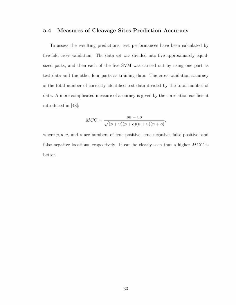
5.4 Measures of Cleavage Sites Prediction Accuracy
To assess the resulting predictions, test performances have been calculated by
five-fold cross validation. The data set was divided into five approximately equal-
sized parts, and then each of the five SVM was carried out by using one part as
test data and the other four parts as training data. The cross validation accuracy
is the total number of correctly identified test data divided by the total number of
data. A more complicated measure of accuracy is given by the correlation coefficient
introduced in [48]:
MCC =pn− uo
√
(p + u)(p + o)(n + u)(n + o),
where p, n, u, and o are numbers of true positive, true negative, false positive, and
false negative locations, respectively. It can be clearly seen that a higher MCC is
better.
33

CHAPTER VI
Results
6.1 Comparison of Protein Second Structure Prediction
We carried out some experiments to tune up and evaluate the prediction system
by training 1/7 of the data set and testing the selected model by another 1/7. After
this we find the pair of C = 10 and γ = 0.05 that achieves the best prediction rate.
Therefore, this best parameter set is used for constructing the models for future
testing.
Table 6.1 lists the number of training as well as testing data of the seven cross
validation steps. It also reports the number of support vectors and the accuracy. Note
that numbers of training/testing data are different as our split on the training/testing
sets is at the level of proteins but not amino acids. The average accuracy is 70.5%
which is competitive with results in Rost and Sander [65]. Indeed in [65] a direct use
of neural networks on this encoding scheme achieved only 68.2% accuracy. Other
techniques must be incorporated in order to attain 70% accuracy.
We would like to emphasize here again that we use the same data set (including
the type of alignment profiles) and secondary structure definition (reduction from
eight to three secondary structure) as those in Rost and Sander. In addition, the
same accuracy assessment of Rost and Sander is used so the comparison is fair.
34

For many SVM applications the percentage of training data as support vectors
is quite low. However, here this percentage is very high. That seems to show that
this application is a difficult problem for SVM. As the testing time is proportional
to the number of support vectors, further investigations on how to reduce it remain
to be done.
Table 6.1: SVM for protein secondary structure prediction. Using the seven-foldcross validation on RS130 protein set
Test sets A B C D E F G Total# Test data 4276 3328 3449 3842 2871 2771 3850 24387# Training data 20111 21059 20938 20545 21516 21616 20537# Support vectors 15669 16738 16487 16242 16960 17044 16235Test accuracy% 66.6 73.4 72.9 69.7 71.6 71.3 69.3 70.5
We also test a different SVM formulation:
minw,b,ξ
12wT w + C(
l∑
i=1
ξ2i )
yi((wT φ(xi)) + b) ≥ 1− ξi, (6.1)
ξi ≥ 0, i = 1, . . . , l.
It differs from (2.2) on the penalty term where a quadratic one is used. This was
first proposed in [14] and has been tested in several work (e.g. [39]). Generally (6.1)
can achieve as good accuracy as (2.2) though the number of support vectors may be
larger. The results of using (6.1) are in Table 6.2. The test accuracy is similar to
that in Table 6.1 though the number of support vectors is higher.
Table 6.2: SVM for protein secondary structure prediction. Using the quadraticpenalty term and the seven-fold cross validation on RS130 protein set
Test sets A B C D E F G Total# Support vectors 17192 18261 18044 17642 18553 18599 17679Test accuracy% 66.72 73.95 72.60 69.81 71.79 70.52 69.14 70.44
35
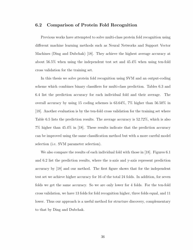
6.2 Comparison of Protein Fold Recognition
Previous works have attempted to solve multi-class protein fold recognition using
different machine learning methods such as Neural Networks and Support Vector
Machines (Ding and Dubchak) [18]. They achieve the highest average accuracy at
about 56.5% when using the independent test set and 45.4% when using ten-fold
cross validation for the training set.
In this thesis we solve protein fold recognition using SVM and an output-coding
scheme which combines binary classifiers for multi-class prediction. Tables 6.3 and
6.4 list the prediction accuracy for each individual fold and their average. The
overall accuracy by using 15 coding schemes is 63.64%, 7% higher than 56.50% in
[18]. Another evaluation is by the ten-fold cross validation for the training set where
Table 6.5 lists the prediction results. The average accuracy is 52.72%, which is also
7% higher than 45.4% in [18]. These results indicate that the prediction accuracy
can be improved using the same classification method but with a more careful model
selection (i.e. SVM parameter selection).
We also compare the results of each individual fold with those in [18]. Figures 6.1
and 6.2 list the prediction results, where the x-axis and y-axis represent prediction
accuracy by [18] and our method. The first figure shows that for the independent
test set we achieve higher accuracy for 16 of the total 24 folds. In addition, for seven
folds we get the same accuracy. So we are only lower for 4 folds. For the ten-fold
cross validation, we have 13 folds for fold recognition higher, three folds equal, and 11
lower. Thus our approach is a useful method for structure discovery, complementary
to that by Ding and Dubchak.
36

Table 6.3: Prediction accuracy Qi for protein fold in percentage for the independenttest set
Fold C S H V P Z CS HZ1 83.3 66.7 33.3 50.0 .0 50.0 66.7 50.03 11.1 11.1 22.2 22.2 22.2 11.1 66.7 22.24 30.0 40.0 20.0 30.0 20.0 15.0 50.0 20.07 37.5 37.5 12.5 25.0 12.5 25.0 25.0 12.59 100.0 55.6 44.4 33.3 55.6 44.4 100.0 33.311 55.6 .0 .0 .0 11.1 .0 .0 .020 34.1 22.7 20.5 15.9 15.9 20.5 31.8 20.523 16.7 8.3 8.3 16.7 .0 8.3 8.3 8.326 30.8 7.7 15.4 7.7 .0 .0 7.7 38.530 33.3 16.7 16.7 16.7 16.7 16.7 16.7 16.731 25.0 .0 25.0 12.5 25.0 12.5 25.0 25.032 15.8 15.8 21.1 21.1 15.8 21.1 15.8 31.633 25.0 50.0 25.0 25.0 25.0 50.0 25.0 50.035 25.0 25.0 25.0 25.0 25.0 25.0 25.0 25.039 57.1 28.6 28.6 28.6 .0 28.6 28.6 28.646 22.9 22.9 16.7 20.8 16.7 20.8 50.0 39.647 33.3 58.3 25.0 25.0 25.0 25.0 58.3 25.048 15.4 15.4 15.4 15.4 15.4 15.4 15.4 15.451 18.5 7.4 11.1 18.5 11.1 18.5 25.9 18.554 33.3 25.0 25.0 16.7 16.7 33.3 25.0 33.357 25.0 37.5 25.0 12.5 37.5 12.5 37.5 25.059 42.9 42.9 42.9 14.3 35.7 28.6 35.7 35.762 14.3 14.3 14.3 14.3 14.3 14.3 14.3 28.669 25.0 25.0 .0 .0 .0 .0 25.0 25.072 25.0 12.5 12.5 12.5 25.0 12.5 12.5 25.087 3.7 11.1 14.8 14.8 14.8 18.5 14.8 14.8110 88.9 59.3 40.7 48.1 7.4 51.9 88.9 51.9Avg 32.7 25.5 20.8 20.8 16.4 21.8 36.1 27.3
37

Table 6.4: (Cont’d) Prediction accuracy Qi for protein fold in percentage for theindependent test set
Fold SV CSH VPZ HVP CSHV CSHVPZ 1-vs-1 ALL1 66.7 66.7 50.0 66.7 66.7 66.7 66.7 83.33 33.3 66.7 11.1 11.1 66.7 66.7 77.8 77.84 30.0 40.0 15.0 10.0 35.0 25.0 35.0 65.07 12.5 37.5 25.0 12.5 37.5 37.5 50.0 62.59 55.6 100.0 33.3 11.1 100.0 88.9 88.9 100.011 .0 .0 .0 .0 .0 .0 33.3 55.620 20.5 43.2 20.5 29.5 .0 43.2 84.1 86.423 8.3 8.3 8.3 8.3 8.3 8.3 25.0 25.026 .0 .0 61.5 7.7 7.7 7.7 69.2 69.230 16.7 16.7 16.7 16.7 16.7 16.7 33.3 33.331 12.5 12.5 12.5 25.0 12.5 12.5 50.0 50.032 15.8 15.8 21.1 21.1 15.8 15.8 36.8 36.833 25.0 25.0 25.0 25.0 50.0 25.0 75.0 75.035 25.0 25.0 25.0 25.0 25.0 25.0 25.0 25.039 28.6 28.6 28.6 42.9 28.6 28.6 42.9 42.946 43.8 41.7 20.8 20.8 39.6 37.5 89.6 87.547 58.3 41.7 25.0 25.0 58.3 50.0 66.7 66.748 23.1 30.8 15.4 15.4 23.1 15.4 30.8 38.551 22.2 22.2 18.5 18.5 22.2 18.5 37.0 37.054 25.0 33.3 33.3 33.3 33.3 33.3 50.0 50.057 37.5 37.5 12.5 25.0 37.5 50.0 62.5 62.559 35.7 35.7 35.7 35.7 28.6 28.6 50.0 57.162 14.3 14.3 14.3 14.3 14.3 28.6 57.1 71.469 25.0 25.0 25.0 25.0 .0 25.0 .0 50.072 25.0 12.5 12.5 12.5 12.5 25.0 25.0 25.087 14.8 11.1 18.5 14.8 11.1 11.1 40.7 40.7110 55.6 81.5 88.9 74.1 70.4 70.4 81.5 100.0Avg 28.3 34.8 26.5 24.4 28.8 32.7 58.2 63.6
38

Table 6.5: Prediction accuracy Qi for protein fold in percentage for the ten-fold crossvalidation.
Fold C S CS SV CSH CSHV CSHVPZ 1-vs-1 ALL1 38.5 23.1 38.5 30.8 53.8 30.8 30.8 61.5 69.23 14.3 .0 14.3 .0 14.3 .0 .0 57.1 57.14 25.0 8.3 8.3 16.7 16.7 33.3 33.3 41.7 50.07 14.3 14.3 57.1 57.1 57.1 57.1 71.4 42.9 85.79 22.2 11.1 11.1 11.1 .0 .0 11.1 22.2 33.311 14.3 28.6 28.6 42.9 42.9 42.9 14.3 57.1 71.420 26.7 13.3 30.0 16.7 26.7 23.3 26.7 36.7 46.723 .0 .0 11.1 11.1 .0 11.1 11.1 33.3 22.226 43.8 18.8 37.5 31.3 37.5 25.0 37.5 56.3 68.830 .0 14.3 28.6 42.9 14.3 14.3 14.3 28.6 42.931 12.5 .0 .0 .0 .0 .0 12.5 25.0 25.032 38.5 15.4 38.5 15.4 23.1 23.1 30.8 46.2 61.533 .0 .0 .0 12.5 .0 12.5 12.5 50.0 50.035 11.1 11.1 11.1 22.2 11.1 .0 .0 11.1 11.139 44.4 33.3 66.7 44.4 55.6 44.4 44.4 44.4 66.746 17.2 17.2 31.0 27.6 27.6 20.7 17.2 34.5 44.847 27.3 18.2 18.2 18.2 18.2 18.2 27.3 36.4 54.548 9.1 27.3 45.5 36.4 27.3 27.3 18.2 54.5 72.751 30.8 23.1 46.2 38.5 46.2 30.8 38.5 53.8 53.854 30.0 10.0 20.0 30.0 30.0 40.0 30.0 50.0 60.057 .0 .0 .0 .0 .0 .0 .0 11.1 11.159 50.0 20.0 30.0 40.0 40.0 40.0 30.0 50.0 80.062 18.2 18.2 27.3 18.2 27.3 .0 18.2 45.5 63.669 .0 27.3 45.5 36.4 54.5 45.5 36.4 18.2 54.572 14.3 28.6 57.1 42.9 57.1 42.9 57.1 14.3 71.487 15.4 15.4 15.4 15.4 23.1 15.4 23.1 46.2 53.8110 21.4 28.6 35.7 42.9 35.7 28.6 28.6 35.7 50.0Avg 21.7 16.3 28.8 25.6 28.1 23.3 25.2 39.9 52.7
We do not list the parameter sets, which average accuracy below than 20%
39

� � � � � � � � � � � � � � � � � � � � � � � � � � � � � � � � � � � � � � � � � � � � � � � � � � � �
�� �
� �� �
� �� �
� �� �
� � �
� � �
� �� ! "
#! $%&""
'�&"(
)* $
'�+�
#, $ -
. / 0 1 2 3 4 5 / 6 / 7 1 3 8 9 4 : ; 4 / 6 2 : : < 3 2 : => 4 ; ? @ A 7 / B 9 : B 2 5 5 8 5
C 6 9 8 1 8 6 9 8 6 ; ; 8 5 ; 5 8 ;
Figure 6.1: A comparison of 27 folds for independent test set
� � � � � � � � � � � � � � � � � � � � � � � � � � � � � � � � � � � � � � � � � � � � � � � � � � � �
�� �
� �� �
� �� �
� �� �
� � �
� � �
� �� ! "
#! $%&""
'�&"(
)* $
'�+�
#, $ - . / 0 1 2 3 4 5 / 6 / 7 1 3 8 9 4 : ; 4 / 6 2 : : < 3 2 : => 4 ; ? @ A 7 / B 9 : B 2 5 5 8 5
C D E 7 / B 9 : 3 / 5 5 F 2 B 4 9 2 ; 4 / 6
Figure 6.2: A comparison of 27 folds for ten-fold cross validation
40

6.3 Comparison of Signal Peptide Cleavage Sites Prediction
We use the five-fold cross validation on different parameters for the model selec-
tion. That is, data set is separated into five approximately equal-sized parts, and
then three SVMs are sequentially solved by using one group for testing the rest for
training. Average of the five testing accuracy is treated as our estimation. Results
are in Table 6.6 where we list the best parameters C and γ.
Table 6.6: The best parameters C and γ chosen for each subsystem and the combiner
Model C γ Total accuracy%Subsystem 1 10 0.012 95.6512Subsystem 2 15 0.006 95.7168Subsystem 3 4 0.007 96.0664Subsystem 4 10 0.200 95.0612SVM combiner 10 0.050 96.7657
Accuracy for subsystems 1-4 and SVM combiner is by five-fold cross validation.
Most tools currently available use artificial neural networks, such as SignalP,
(version 1.0) ([55, 56]) and the adaptive encoding artificial neural network (ACN)
([33]). We compare the proposed approach with them by using all 416 positive and
4160 negative patterns.
The comparison between earlier results and our SVM approach is in Table 6.3.
Using SVM combiner, the overall performance ((p + n)/(p + u + n + o)) is 96.8%,
which improves the results by SignalP and ACN. Accuracy for cleavage site location
is 84.1%, which also improves the results by SignalP and ACN. The correlation
coefficient ([48]) using the SVM combiner is 0.81, which mean that over-prediction
is lower for the SVM than for SignalP and ACN. On the other hand, using SVM a
predicted cleavage site is more likely to be a true cleavage site.
41
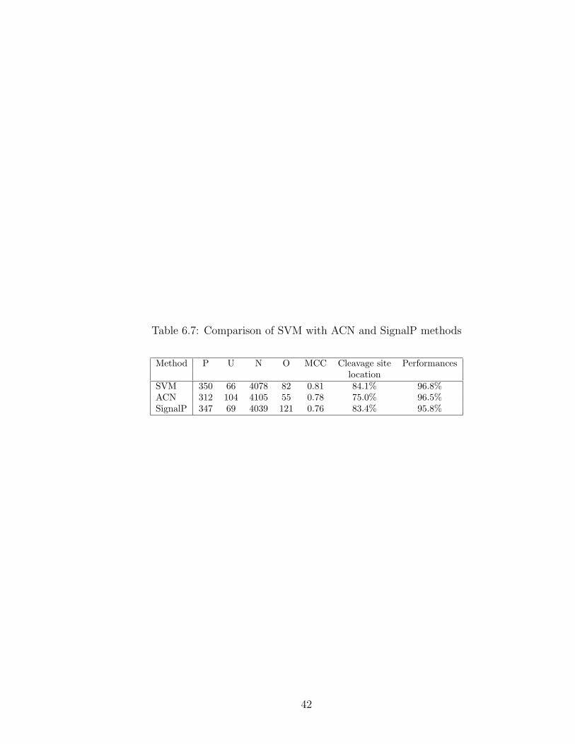
Table 6.7: Comparison of SVM with ACN and SignalP methods
Method P U N O MCC Cleavage site Performanceslocation
SVM 350 66 4078 82 0.81 84.1% 96.8%ACN 312 104 4105 55 0.78 75.0% 96.5%SignalP 347 69 4039 121 0.76 83.4% 95.8%
42
CHAPTER VII
Conclusions and Discussions
7.1 Protein Secondary Structure Prediction
Using SVM for protein secondary structure prediction, we achieve a comparable
performance through seven-fold cross validation on a database used by Rost and
Sander [65].
It has been shown by many researchers that using more data improves the accu-
racy for prediction. We have a similar observation while using SVM. The improve-
ment may be due to the accidental addition of more easily predicted sequences to
the set or better predictive patterns learned by the classifiers trained on more se-
quences. In the future, we will try to use a larger data set and may further increase
the prediction accuracy.
Here we experiment with only basic features of SVM. There are other possibilities
to improve its performance. We plan to work on reducing the training time, so
that more options and features of SVM can be tried in order to obtain further
improvements.
43
7.2 Multi-class Protein Fold Recognition
Predicting a protein from one of 27 folding classes is very difficult because of the
similarity among different classes. Here we present a computational method based
on SVM for the assignment of a protein sequence to a folding class in the SCOP
database.
Applying our method increases the overall prediction accuracy to 63.6% when
using an independent test set and 52.7% when using the ten-fold cross validation on
the training set. Both improve the current prediction accuracy by more than 7%.
The experimental results reveal that model selection is an important step in SVM
design. For a large number of classes and highly unbalanced data, a careful selection
of the optimal hyperparameters for each binary classifier will improve accuracy. In
the future, we will try to use our method to other problems of this type.
7.3 Signal Peptide Cleavage Sites Prediction
Using SVM for the recognition of human signal peptide cleavage sites, the overall
performance is 96.8%, which improves the results in SignalP and ACN. Accuracy for
cleavage site location is 84.1%, which also improves the results by SignalP and ACN.
The correlation coefficient is 0.81, which mean that overprediction is lower for the
SVM than for SignalP and ACN.
The experimental results reveal that SVM can easily achieve comparable accuracy
as other predictors. Thus SVM can be a powerful computational tool for predicting
the signal peptide cleavage sites. Therefore, it is a promising direction to study other
applications by using SVM.
44

APPENDICES
45

APPENDIX A
Optimal Hyperparameters for Protein FoldRecognition
46

Table A.1: Optimal hyperparameters for the training set by 10-fold cross validation.
fold Comp. S H V P Z CSindex C γ C γ C γ C γ C γ C γ C γ1 50 50 50 50 10 1000 10 50 10 0.01 10 100 10 103 1 1000 1 10 10 50 10 10 10 100 10 10 50 14 10 10 10 10 10 50 10 10 10 50 1 100 1000 0.17 10 100 10 50 10 10 10 50 10 10 10 100 10 109 10 50 10 50 10 100 10 100 10 50 10 50 500 0.111 10 50 1 1 1 1 1 1 10 50 1 1 1 120 10 10 1 10 10 100 1 100 10 1000 10 100 100 0.123 10 100 1 50 10 10 10 10 1 1 10 10 1 1026 1 100 100 50 10 100 10 100 1 1 1 1 10 5030 10 100 10 100 10 50 10 1000 10 100 10 10 1 5031 10 10 1 1 100 50 1 50 10 50 1 100 1000 0.0132 10 1000 10 50 10 100 10 50 10 50 10 50 10 5033 10 10 10 50 10 10 1 100 1 100 10 50 1 5035 10 100 1 50 1 50 1 50 1 50 10 50 1 1039 10 50 10 10 10 100 10 100 1 1 10 100 10 1046 10 1000 10 50 1 1000 10 1000 1 1000 50 1000 50 1047 10 1000 10 10 10 1000 10 1000 10 1000 10 1000 10 1048 10 1000 10 100 10 1000 10 50 10 1000 1 100 1 5051 10 1000 10 1 1 1000 10 100 1 1000 10 100 50 1054 10 100 10 50 1000 0.1 10 1000 10 10 10 100 10 5057 10 100 10 10 10 10 1 1000 10 50 10 50 10 159 10 1000 10 10 10 100 1 1000 10 100 10 100 10 1062 1 1000 1 100 1 100 10 10 1 1000 10 10 1 5069 10 50 100 50 1 1 1 1 1 1 1 1 10 1072 10 100 10 50 10 50 10 50 10 10 10 50 10 5087 500 1 1 50 10 50 10 50 10 100 10 50 10 10110 10 10 500 0.1 500 0.1 10 1 1 50 1000 1 500 0.1
47

Table A.2: (Cont’d) Optimal hyperparameters for the training set by 10-fold crossvalidation.
fold HZ SV CSH VPZ HVP CSHV CSHVPZindex C γ C γ C γ C γ C γ C γ C γ1 10 10 10 10 10 10 10 10 10 10 10 1 10 503 50 0.1 10 1 1 50 100 0.1 10 1 10 1 50 104 50 0.1 10 1 50 0.1 50 0.1 50 0.1 10 1 1000 107 1 50 10 1 50 10 1 50 10 1 10 1 10 509 10 10 500 0.1 10 50 100 0.1 500 0.01 500 0.01 500 5011 1 1 1 1 1 1 1 1 1 1 1 1 1 120 50 10 100 0.1 10 50 10 10 10 0.1 10 1 100 5023 1 10 1 10 10 10 10 10 1 10 10 10 1 1026 1 1 1 1 10 10 10 50 10 10 10 10 10 1030 10 10 10 10 10 50 10 50 10 10 1 10 1 1031 1 10 1 50 1 50 10 10 1 10 1 10 1000 1032 10 10 10 10 10 10 10 10 10 10 10 10 10 1033 1 50 1 50 1 50 1 50 1000 0.01 1 10 1 1035 1 10 1 10 10 10 1 10 10 1 10 1 1 1039 10 1 10 1 10 50 10 10 10 1 10 1 10 5046 10 10 10 10 1 50 1 50 10 10 10 10 50 5047 50 1 10 1 1 100 1 100 50 1 50 1 10 5048 10 10 10 10 1 50 1 50 10 10 1 10 1 5051 10 10 10 10 10 50 10 10 10 1 10 10 50 5054 10 50 10 10 10 50 10 50 10 10 10 10 10 5057 50 1 10 1 1 50 10 10 50 0.1 50 0.1 10 1059 10 10 10 10 10 50 10 50 10 10 10 10 10 5062 1 50 1 50 1 50 1 50 1 10 10 10 1 5069 10 10 10 10 10 50 1 50 10 10 10 10 10 5072 10 10 10 10 10 1 10 10 10 10 10 1 10 1087 10 10 10 10 10 10 10 10 10 10 10 10 10 10110 50 0.1 500 0.01 100 0.1 500 0.01 50 0.1 50 0.1 500 1
48
APPENDIX B
Data Set for Human Signal Peptide Cleavage SitesPredictions
Table B.1: Data set for human signal peptide cleavage sites prediction
10KS-HUMAN 1B05-HUMAN 5NTD-HUMAN 7B2-HUMAN A1AH-HUMANA1AT-HUMAN A2AP-HUMAN A2HS-HUMAN A4-HUMAN AACT-HUMANABP-HUMAN ACET-HUMAN ACE-HUMAN ACHA-HUMAN ACHB-HUMANACHE-HUMAN ACHG-HUMAN ACHN-HUMAN ACRO-HUMAN ALBU-HUMANALK1-HUMAN ALS-HUMAN AMYP-HUMAN ANF-HUMAN ANGI-HUMANANGT-HUMAN ANPA-HUMAN ANPC-HUMAN ANT3-HUMAN APA1-HUMANAPA2-HUMAN APA4-HUMAN APC1-HUMAN APC2-HUMAN APC3-HUMANAPD-HUMAN APE-HUMAN APOA-HUMAN APOH-HUMAN ARSA-HUMANASM-HUMAN ASPG-HUMAN AXO1-HUMAN B2MG-HUMAN B61-HUMANB71-HUMAN BAL-HUMAN BFR2-HUMAN BGAM-HUMAN BGLR-HUMANBLSA-HUMAN C1QA-HUMAN C1QC-HUMAN C1R-HUMAN C1S-HUMANC4BB-HUMAN C4BP-HUMAN CA11-HUMAN CA13-HUMAN CA14-HUMANCA18-HUMAN CA19-HUMAN CA21-HUMAN CA24-HUMAN CA25-HUMANCAH4-HUMAN CAH6-HUMAN CAMA-HUMAN CAML-HUMAN CAP7-HUMANCASB-HUMAN CASK-HUMAN CATD-HUMAN CATE-HUMAN CATH-HUMANCATL-HUMAN CBG-HUMAN CBP1-HUMAN CBPB-HUMAN CBPC-HUMANCBPN-HUMAN CCKN-HUMAN CD14-HUMAN CD1A-HUMAN CD1D-HUMANCD1E-HUMAN CD28-HUMAN CD2-HUMAN CD30-HUMAN CD3D-HUMANCD3E-HUMAN CD3G-HUMAN CD3Z-HUMAN CD45-HUMAN CD4X-HUMANCD4-HUMAN CD52-HUMAN CD59-HUMAN CD5-HUMAN CD7-HUMANCD82-HUMAN CD8A-HUMAN CERU-HUMAN CETP-HUMAN CFAI-HUMANCHLE-HUMAN CLUS-HUMAN CMGA-HUMAN CO2-HUMAN CO3-HUMANCO4-HUMAN CO6-HUMAN CO7-HUMAN CO8G-HUMAN COG1-HUMANCOG7-HUMAN COG8-HUMAN COG9-HUMAN COL-HUMAN CR1-HUMANCR2-HUMAN CRFB-HUMAN CRTC-HUMAN CSF1-HUMAN CSF2-HUMANCSF3-HUMAN CTRB-HUMAN CYPB-HUMAN CYRG-HUMAN CYTC-HUMANCYTS-HUMAN DAF2-HUMAN DEFN-HUMAN DOPO-HUMAN DRN1-HUMANE2-HUMAN EGFR-HUMAN EL2B-HUMAN ELS-HUMAN EMBP-HUMANENPL-HUMAN EPOR-HUMAN EPO-HUMAN F13B-HUMAN FA12-HUMANFA5-HUMAN FA8-HUMAN FBLB-HUMAN FCEA-HUMAN FCG1-HUMANFETA-HUMAN FGF7-HUMAN FGR3-HUMAN FIBA-HUMAN FIBB-HUMANFIBH-HUMAN FINC-HUMAN FKB3-HUMAN FOL2-HUMAN FSA-HUMANFSHB-HUMAN GA6S-HUMAN GELS-HUMAN GL6S-HUMAN GLCM-HUMANGLHA-HUMAN GLPE-HUMAN GLUC-HUMAN GLYP-HUMAN GMCR-HUMANGONL-HUMAN GP1A-HUMAN GP1B-HUMAN GP39-HUMAN GPIX-HUMANGR78-HUMAN GRA1-HUMAN GRAA-HUMAN GRP2-HUMAN GUAN-HUMANHA25-HUMAN HA2R-HUMAN HA2Z-HUMAN HB23-HUMAN HB2A-HUMANHB2Q-HUMAN HC-HUMAN HEP2-HUMAN HEXA-HUMAN HGFA-HUMANHGF-HUMAN HIS3-HUMAN HPT2-HUMAN HRG-HUMAN HV1B-HUMANHV2H-HUMAN HV2I-HUMAN HV3C-HUMAN I12A-HUMAN I12B-HUMANI309-HUMAN IAC2-HUMAN IBP1-HUMAN IBP2-HUMAN IBP3-HUMANIBP4-HUMAN IC1-HUMAN ICA1-HUMAN ICA2-HUMAN IGF2-HUMAN
49

Table B.2: (Cont’d) Data set for human signal peptide cleavage sites prediction
IHA-HUMAN IHBA-HUMAN IL11-HUMAN IL1R-HUMAN IL1X-HUMANIL2A-HUMAN IL2B-HUMAN IL2-HUMAN IL3-HUMAN IL4-HUMANIL5R-HUMAN IL5-HUMAN IL6R-HUMAN IL6-HUMAN IL7R-HUMANIL7-HUMAN IL8-HUMAN IL9-HUMAN INA7-HUMAN INB-HUMANINGR-HUMAN ING-HUMAN INIG-HUMAN INIP-HUMAN INSR-HUMANINS-HUMAN IPSP-HUMAN IPST-HUMAN IRBP-HUMAN ITA2-HUMANITA4-HUMAN ITA6-HUMAN ITAB-HUMAN ITAL-HUMAN ITAV-HUMANITAX-HUMAN ITB1-HUMAN ITB2-HUMAN ITB4-HUMAN ITB7-HUMANKAL-HUMAN KFMS-HUMAN KHEK-HUMAN KKIT-HUMAN KMET-HUMANKNL-HUMAN KV4B-HUMAN KV5A-HUMAN LAG3-HUMAN LBP-HUMANLCAT-HUMAN LCA-HUMAN LDLR-HUMAN LEM1-HUMAN LEM3-HUMANLEUK-HUMAN LFA3-HUMAN LIF-HUMAN LIPG-HUMAN LIPH-HUMANLIPL-HUMAN LIPP-HUMAN LITH-HUMAN LMB1-HUMAN LMB2-HUMANLMP1-HUMAN LMP2-HUMAN LPH-HUMAN LSHB-HUMAN LV0A-HUMANLV6E-HUMAN LYC-HUMAN LYSH-HUMAN MABC-HUMAN MAG-HUMANMCPI-HUMAN MCP-HUMAN MDP1-HUMAN MG24-HUMAN MGP-HUMANMI1B-HUMAN MI2B-HUMAN MK-HUMAN MLCH-HUMAN MOTI-HUMANMPRD-HUMAN MPRI-HUMAN MYP0-HUMAN NAGA-HUMAN NCA2-HUMANNDDB-HUMAN NEC2-HUMAN NEU2-HUMAN NEUB-HUMAN NGFR-HUMANNIDO-HUMAN NMZ2-HUMAN OMGP-HUMAN ONCM-HUMAN P4HA-HUMANPA21-HUMAN PA2M-HUMAN PAHO-HUMAN PAI1-HUMAN PBGD-HUMANPDGB-HUMAN PEC1-HUMAN PENK-HUMAN PEPA-HUMAN PEPC-HUMANPERF-HUMAN PF4L-HUMAN PGDR-HUMAN PGDS-HUMAN PGH1-HUMANPGSG-HUMAN PLFV-HUMAN PLMN-HUMAN PLR2-HUMAN PP11-HUMANPP14-HUMAN PPA5-HUMAN PPAL-HUMAN PPAP-HUMAN PPB3-HUMANPPBT-HUMAN PRIO-HUMAN PRL-HUMAN PRN3-HUMAN PROP-HUMANPRPC-HUMAN PRTC-HUMAN PRTP-HUMAN PRTS-HUMAN PRTZ-HUMANPS2-HUMAN PSPA-HUMAN PSSP-HUMAN PTHY-HUMAN PTN-HUMANPTPG-HUMAN PZP-HUMAN REL2-HUMAN RENI-HUMAN RETB-HUMANRIB1-HUMAN RIB2-HUMAN RNKD-HUMAN SAA-HUMAN SABP-HUMANSAMP-HUMAN SAP3-HUMAN SAP-HUMAN SCF-HUMAN SEM2-HUMANSG1-HUMAN SIAL-HUMAN SLIB-HUMAN SMS1-HUMAN SODE-HUMANSOMW-HUMAN SPRC-HUMAN SRCH-HUMAN SSBP-HUMAN STAT-HUMANSTS-HUMAN TCO1-HUMAN TCO2-HUMAN TENA-HUMAN TETN-HUMANTFPI-HUMAN TF-HUMAN TGR3-HUMAN THBG-HUMAN THY1-HUMANTHYG-HUMAN TIM2-HUMAN TNFB-HUMAN TNR1-HUMAN TNR2-HUMANTRFE-HUMAN TRFL-HUMAN TRFM-HUMAN TRKA-HUMAN TRY2-HUMANTRYA-HUMAN TSHB-HUMAN TSHR-HUMAN TSP1-HUMAN TTHY-HUMANTVA2-HUMAN TVA3-HUMAN TVB2-HUMAN TVC-HUMAN TYRR-HUMANUPAR-HUMAN UROK-HUMAN UROM-HUMAN VEGF-HUMAN VIP-HUMANVTDB-HUMAN VTNC-HUMAN VWF-HUMAN WNT1-HUMAN ZA2G-HUMANZP2-HUMAN
50

BIBLIOGRAPHY
[1] P. Baldi, S. Brunak, P. Frasconi, G. Soda, and G. Pollastri. Exploiting thepast and the future in protein secondary structure prediction. Bioinformatics,15:937–946, 1999.
[2] K. P. Bennett, D. Hui, and L. Auslender. On support vector decision trees fordatabase marketing. Department of Mathematical Sciences Math Report No.98-100, Rensselaer Polytechnic Institute, Troy, NY 12180, Mar. 1998.
[3] V. Biou, J.-F. Gibrat, J. Levin, B. Robson, and J. Garnier. Secondary structureprediction: combination of three different methods. Protein Engineering, 2:185–191, 1989.
[4] H. Bohr, J. Bohr, S. Brunak, R. Cotterill, B. Lautrup, L. Nskov, O. Olsen, andS. Petersen. Protein secondary structures and homology by neural networks:The helices in rhodopsin. FEBS Letters, 241:223–228, 1988.
[5] B. Boser, I. Guyon, and V. Vapnik. A training algorithm for optimal mar-gin classifiers. In Proceedings of the Fifth Annual Workshop on ComputationalLearning Theory, 1992.
[6] M. Brown, W. Grundy, D. Lin, N. Cristianini, C. Sugnet, M. Ares, and D. Haus-sler. Support vector machine classification of microarray gene expression data.Technical Report UCSC-CRL-99-09, University of California, Santa Cruz, 1999.
[7] M. P. S. Brown, W. N. Grundy, D. Lin, N. Cristianini, C. Sugnet, T. S. Furey,J. M.Ares, and D. Haussler. Knowledge-based analysis of microarray gene ex-pression data using support vector machines. PNAS, 97(1):262–267, 2000.
[8] C. J. C. Burges. A tutorial on support vector machines for pattern recognition.Data Mining and Knowledge Discovery, 2(2):121–167, 1998.
[9] J.-M. Chandonia and M. Karplus. Neural networks for secondary structure andstructural class predictions. Prot. Sci., 4:275–285, 1995.
[10] C.-C. Chang and C.-J. Lin. LIBSVM: a library for support vector machines,2001. Software available at http://www.csie.ntu.edu.tw/~cjlin/libsvm.
[11] C. Chothia and A. V. Finkelstein. The classification and origin of protein foldingpatterns. Annu. Rev. Biochem., 59:1007–1039, 1990.
51
[12] F. E. Cohen and I. D. Kuntz. Tertiary Structure Prediction. In Prediction ofprotein structure and the principles of protein conformation. Plenum Press, NewYork, London., 1989.
[13] L. L. Conte, B. Ailey, T. J. P. Hubbard, S. E. Brenner, A. G. Murzin, andC. Chothia. SCOP: a structure classification of proteins database. NucleicAcids Res., 28:257–259, 2000.
[14] C. Cortes and V. Vapnik. Support-vector network. Machine Learning, 20:273–297, 1995.
[15] N. Cristianini and J. Shawe-Taylor. An Introduction to Support Vector Ma-chines. Cambridge University Press, Cambridge, UK, 2000.
[16] J. A. Cuff and G. J. Barton. Evalution and improvement of multiple sequencemethods for protein secondary structure prediction. Proteins: Struct. Funct.Genet., 34:508–519, 1999.
[17] D. DeCoste and B. Scholkopf. Training invariant support vector machines. Ma-chine Learning, 2001. To appear.
[18] C. H. Q. Ding and I. Dubchak. Multi-class protein fold recognition using supportvector machines and neural networks. Bioinformatics, 17(4):349–358, 2001.
[19] D. Donnelly, J. P. Overington, and T. L. Blundell. The prediction and orienta-tion of a-helices from sequence alignments: the combined use of environment-dependent substitution tables, fourier transform methods and helix cappingrules. Prot. Engin., 7:645–653, 1994.
[20] K. Duan, S. S. Keerthi., and A. N. Poo. Evaluation of simple performance mea-sures for tuning svm hyperparameters. Technical Report CD-01-11, Departmentof Mechanical Engineering National University of Singapore, 2001.
[21] I. Dubchak, I. Muchnik, S. R. Holbrook, and S. H. Kim. Prediction of proteinfolding class using global description of amino acid sequence. Proc. Natl Acad.Sci. USA, 92:8700–8704, 1995.
[22] I. Dubchak, I. Muchnik, C. Mayor, I. Dralyuk, and S. H. Kim. Recognition ofa protein fold in the context of the structural classification of protein (SCOP)classification. Proteins, 35:401–407, 1999.
[23] J. Friedman. Another approach to polychotomous classification. Techni-cal report, Department of Statistics, Stanford University, 1996. Available athttp://www-stat.stanford.edu/reports/friedman/poly.ps.Z.
[24] D. Frishman and P. Argos. Knowledge-based protein secondary structure as-signment. Proteins, 23:566–579, 1995.
52
[25] J. Garnier, D. Osguthorpe, and B. Robson. Analysis of the accuracy and im-plications of simple methods for predicting the secondary structure of globularproteins. Journal of Molecular Biology, 120:97–120, 1978.
[26] O. Gascuel and J. L. Golmard. A simple method for predicting the secondarystructure of globular proteins: implications and accuracy. CABIOS, 4:357–365,1988.
[27] C. Geourjon and G. Deleage. Sopma: significant improvements in protein sec-ondary structure prediction by consensus prediction from multiple alignments.CABIOS, 11:681–684, 1995.
[28] J.-F. Gibrat, J. Garnier, and B. Robson. Further developments of protein sec-ondary structure prediction using information theory. Journal of MolecularBiology, 198:425–443, 1987.
[29] U. Hobohm and C. Sander. Enlarged representative set of proteins. ProteinSci., 3:522–524, 1994.
[30] H. Holley and M. Karplus. Protein secondary structure prediction with a neuralnetwork. In Proceedings of the National Academy of Sciences of the UnitedStates of America, volume 86, pages 152–156, 1989.
[31] C.-W. Hsu and C.-J. Lin. A comparison of methods for multi-class supportvector machines. IEEE Trans. Neural Networks, 2002. To appear.
[32] T. J. P. Hubbard, A. G. Murzin, S. E. Brenner, and C. Chothia. Scop: astructure classification on proteins database. Nucleic Acids Research, 25:236–239, 1997.
[33] B. Jagla and J. Schuchhardt. Adaptive encoding neural networks for the recog-nition of human signal peptide cleavage sites. Bioinformatics, 16(3):245–250,2000.
[34] T. Joachims. Transductive inference for text classification using support vectormachines. In Proceedings of International Conference on Machine Learning,1999.
[35] T. Joachims. The Maximum-Margin Approach to Learning Text Classifiers:Methods, Theory, and Algorithms. PhD thesis, Universitaet Dortmund, 2000.
[36] D. Juretic, B. Lee, N. Trinajstic, and R. W. Williams. Conformational prefer-ence functions for predicting helices in membrane proteins. Biopolymers, 33:255–273, 1993.
[37] W. Kabsch and C. Sander. Dictionary of protein secondary structure: Pat-tern recognition of hydrogen-bonded and geometrical features. Biopolymers,22:2577–2637, 1983.
53

[38] M. Kanehisa. A multivariate analysis method for discriminating protein sec-ondary structural segments. Prot. Engin., 2:87–92, 1988.
[39] S. S. Keerthi, C. B. S. K. Shevade, and K. R. K. Murthy. A fast iterative near-est point algorithm for support vector machine classifier design. IEEE Trans.Neural Networks, 11(1):124–136, 2000.
[40] D. G. Kneller, F. E. Cohen, and R. Langridge. Improvements in protein sec-ondary structure prediction by an enhanced neural network. Journal of Molec-ular Biology, 214:171–182, 1990.
[41] S. Knerr, L. Personnaz, and G. Dreyfus. Single-layer learning revisited: a step-wise procedure for building and training a neural network. In J. Fogelman,editor, Neurocomputing: Algorithms, Architectures and Applications. Springer-Verlag, 1990.
[42] U. Kreßel. Pairwise classification and support vector machines. In B. Scholkopf,C. J. C. Burges, and A. J. Smola, editors, Advances in Kernel Methods —Support Vector Learning, pages 255–268, Cambridge, MA, 1999. MIT Press.
[43] Y. LeCun, L. Jackel, L. Bottou, A. Brunot, C. Cortes, J. Denker, H. Drucker,I. Guyon, U. Muller, E. Sackinger, P. Simard, and V. Vapnik. Comparisonof learning algorithms for handwritten digit recognition. In F.Fogelman andP.Gallinari, editors, International Conference on Artificial Neural Networks,pages 53–60, Paris, 1995. EC2 & Cie., 1995.
[44] C.-J. Lin. Formulations of support vector machines: a note from an optimizationpoint of view. Neural Computation, 13(2):307–317, 2001.
[45] A. Lupas, M. V. Dyke, and J. Stock. Predicting coiled coils from protein se-quences. Science, 252:1162–1164, 1991.
[46] R. Maclin and J. Shavlik. Using knowledge-based neural networks to improvealgorithms: Refining the chou-fasman algorithm for protein folding. MachineLearning, 11:195–215, 11.
[47] N. Matic, I. Guyon, J. Denker, and V. Vapnik. Writer adaptation for on-linehandwritten character recognition. In I. C. S. Press, editor, In Second Interna-tional Conference on Pattern Recognition and Document Analysis, pages 187–191, Tsukuba, Japan, 1993.
[48] B. Matthews. Comparison of the predicted and observed secondary structure oft4 phage lysozyme. Biochim. Biophys. Acta, 405:442–451, 1975.
[49] F. R. Maxfield and H. A. Scheraga. Status of empirical methods for the predic-tion of protein backbone topography. Biochem., 15:5138–5153, 1976.
54

[50] E. M. Mitchell, P. J. Artymiuk, D. W. Rice, and P. Willett. Use of techniquesderived from graph theory to compare secondary structure motifs in proteins.Journal of Molecular Biology, 212:151–166, 1992.
[51] S. Muggleton, R. D. King, and M. J. E. Sternberg. Protein secondary structureprediction using logic-based machine learning. Prot. Engin., 5:647–657, 1992.
[52] K.-R. Muller, A. Smola, G. Ratsch, B. Scholkopf, J. Kohlmorgen, and V. Vapnik.Predicting time series with support vector machines. In B. Scholkopf, C. J. C.Burges, and A. J. Smola, editors, Advances in Kernel Methods - Support VectorLearning, pages 243–254, Cambridge, MA, 1999. MIT Press.
[53] K. Nagano. Triplet information in helix prediction applied to the analysis ofsuper-secondary structures. Journal of Molecular Biology, 109:251–274, 1977.
[54] H. Nielsen, S. Brunak, and G. von Heijne. Machine learning approaches for theprediction of signal peptides and other protein sorting signals. Protein Eng.,12:3–9, 1999.
[55] H. Nielsen, J. Engelbrecht, S. Brunak, and G. von Heijne. Identification ofprokaryotic and eukaryotic signal peptides and prediction of their cleavages sites.Protein Eng., 10:1–6, 1997.
[56] H. Nielsen, J. Engelbrecht, S. Brunak, and G. von Heijne. A neural networkmethod for identification of prokaryotic and eukaryotic signal peptides and pre-diction of their cleavages sites. Int. J. Neural. Syst., 8:581–599, 1997.
[57] C. Papageorgiou, M. Oren, and T. Poggio. A general framework for objectdetection. In International Conference on Computer Vision ICCV’98, 1998.
[58] T. N. Petersen, C. Lundegaard, M. Nielsen, H. Bohr, and J. B. et al. Predictionof protein secondary structure at 80% accuracy. Proteins, 41:17–20, 2000.
[59] O. B. Ptitsyn and A. V. Finkelstein. Theory of protein secondary structure andalgorithm of its prediction. Biopolymers, 22:15–25, 1983.
[60] N. Qian and T. Sejnowski. Predicting the secondary structure of globular pro-teins using neural network models. Journal of Molecular Biology, 202(4):865–884, 1988.
[61] B. Robson. Conformational properties of amino acid residues in globular pro-teins. Journal of Molecular Biology, 107:327–356, 1976.
[62] M. J. Rooman, J. P. Kocher, and S. J. Wodak. Prediction of protein backboneconformation based on seven structure assignments: influence of local interac-tions. Journal of Molecular Biology, 221:961–979, 1991.
[63] B. Rost. Protein secondary structure prediction continues to rise, 2000. Avail-able at http://cubic.bioc.columbia.edu/papers/2001 opinion/paper.html.
55

[64] B. Rost and C. Sander. Improved prediction of protein secondary structure byuse of sequence profiles and neural networks. In Proceedings of the NationalAcademy of Sciences of the United States of America, volume 90, pages 7558–7562, 1993.
[65] B. Rost and C. Sander. Prediction of protein secondary structure at better than70% accuracy. Journal of Molecular Biology, 232(2):584–599, 1993.
[66] B. Rost and C. Sander. Third generation prediction of secondary structure.In D. Webster, editor, In Protein structure prediction: methods and protocols,pages 71–95. Humana Press, Totowa, NJ., 2000.
[67] M. Rychetsky, S. Ortmann, and M. Glesner. Construction of a support vectormachine with local experts. In Workshop on Support Vector Machines at theInternational Joint Conference on Artificial Intelligence (IJCAI 99), 1999.
[68] A. A. Salamov and V. V. Solovyev. Prediction of protein secondary structure bycombining nearest-neighbor algorithms and multiple sequence alignment. Jour-nal of Molecular Biology, 247:11–15, 1995.
[69] C. Sander and R. Schneider. Database of homology-derived protein structuresand the structural meaning of sequence alignment. Proteins, 9(1):56–68, 1991.
[70] T. D. Schneider and R. M. Stephens. Sequence logos: A new way to displayconsensus sequences. Nucleic Acids Research, 18:6097–6100, 1990.
[71] B. Scholkopf, C. J. C. Burges, and A. J. Smola, editors. Advances in KernelMethods - Support Vector Learning. MIT Press, Cambridge, MA, 1998.
[72] V. V. Solovyev and A. A. Salamov. Predicting a-helix and b-strand segmentsof globular proteins. CABIOS, 10:661–669, 1994.
[73] M. O. Stitson, A. Gammerman, V. Vapnik, V. Vovk, C. Watkins, and J. Weston.Support vector regression with ANOVA decomposition kernels. In Scholkopfet al. [71], pages 285–292.
[74] P. Stolorz, A. Lapedes, and Y. Xia. Predicting protein secondary structure usingneural net and statistical methods. Journal of Molecular Biology, 225(2):363–377, 1992.
[75] W. R. Taylor and J. M. Thornton. Prediction of super-secondary structure inproteins. Nature, 301:540–542, 1983.
[76] V. Vapnik. The Nature of Statistical Learning Theory. Springer-Verlag, NewYork, NY, 1995.
[77] V. Vapnik. Statistical Learning Theory. Wiley, New York, NY, 1998.
56
[78] V. N. Viswanadhan, B. Denckla, and J. N. Weinstein. New joint predictionalgorithm (q7-jasep) improves the prediction of protein secondary structure.Biochem., 30:11164–11172, 1991.
[79] G. von Heijne. Signal sequences. the limit in variation. J. Mol. Biol., 184:99–105, 1985.
[80] C. H. Yeang, S. Ramaswamy, P. Tamayo, S. Mukherjee, R. M. Rifkin, M. Angelo,M. Reich, E. Lander, J. Mesirov, and T. Golub. Molecular classification ofmultiple tumor types. Bioinformatics, 17:316S–322S, 2001.
[81] C.-H. Yeang, S. Ramaswamy, P. Tamayo, S. Mukherjee, R. M. Rifkin, M. An-gelo, M. Reich, E. Lander, J. Mesirov, and T. Golub. Molecular classificationof multiple tumor types. Bioinformatics: Discovery Note, 1(1):1–7, 2001.
[82] T.-M. Yi and E. S. Lander. Protein secondary structure prediction usingnearest-neigbor methods. Journal of Molecular Biology, 232:1117–1129, 1993.
[83] X. Zhang, J. Mesirov, and D. Waltz. Hybrid system for protein secondarystructure prediction. Journal of Molecular Biology, 225(4):1049–1063, 1992.
[84] Z.-Y. Zhu and T. L. Blundell. The use of amino acid patterns of classifiedhelices and strands in secondary structure prediction. Journal of MolecularBiology, 260:261–276, 1996.
[85] M. J. Zvelebil, G. J. Barton, W. R. Taylor, and M. J. E. Sternberg. Predictionof protein secondary structure and active sites using alignment of homologoussequences. Journal of Molecular Biology, 195:957–961, 1987.
57