application of streamline in australian cities -...

Australasian Transport Research Forum 2015 Proceedings 30 September - 2 October 2015, Sydney, Australia

Publication website: http://www.atrf.info/papers/index.aspx

1

Application of StreamLine in Australian Cities

Michiel Jagersma1, Cameron Reid2, Dr Tomas Potesil3

1,2,3 Suite 3, Ground Floor, 80 Jephson Street, Toowong

Email for correspondence: [email protected]

Abstract

This paper looks at applications of the Zenith Dynamic Traffic Assignment (DTA) model to strategic planning projects in South East Queensland. Zenith DTA models are underpinned by the StreamLine framework within the OmniTRANS software package. These models are created directly from existing macroscopic, strategic models. Rather than integrating microsimulation with mesoscopic models, StreamLine integrates macroscopic and mesoscopic models. As a result of the relatively simple input needs, Zenith DTA model development can be extremely cost and time effective whilst still providing a wide array of detailed outputs, supporting decision-making at both local and state levels.

Over the last ten years, StreamLine has been successfully applied numerous times in The Netherlands (from where the software originates). Typically, the projects cover larger areas, combinations of regional towns and even a national model. This paper will focus on two specific applications of StreamLine in Australia, and will then address the differences between the application of StreamLine in Australia and The Netherlands.

Our paper investigates two models, created from the strategic Zenith Model of South East Queensland. The first case study is a Zenith DTA model of Wembley Road, demonstrating a successful use of the model on a localised study area. The second case study is an application of the Zenith DTA model to a larger managed motorways project.

We also provide insights into the inner workings of these models and present some of the model outputs, including real-time videos generated by the model.

1. Introduction

Traffic assignment models have always played a significant role in assisting traffic planners to predict traffic flows. The most common form of these is the static assignment model, where demand is assigned to a network for a key period of a day. Whilst useful for strategic assessment, a certain level of detail is lost. Bottlenecks will show as oversaturated links but the resulting queues and the effects these have on the rest of the network are not taken into account. Dynamic assignment models overcome these limitations by preventing traffic flows from exceeding capacities (instead allowing queues to form), and by adding a temporal element. The drawback of these models is that they are generally difficult to set up and to calibrate, and are computationally expensive.

This paper looks at the application of the Zenith Dynamic Traffic Assignment (DTA) models utilising the StreamLine module within the modelling software package OmniTRANS. These models are created directly from existing macroscopic, strategic models. Rather than integrating microsimulation with mesoscopic models, StreamLine integrates macroscopic and mesoscopic models. Zenith DTA models require fewer inputs than more complex microscopic models, especially at the intersection level. For this reason, Zenith DTA model development can be extremely cost and time effective whilst still providing a wide array of detailed outputs, supporting decision-making at both local and state levels.

2

2. The Zenith Dynamic Traffic Assignment

2.1 Introduction

The Zenith Dynamic Traffic Assignment (DTA) is part of a set of modelling tools which is currently available inside the OmniTRANS software platform. It builds upon the StreamLine framework and the traffic propagation model MaDAM, a DTA system which runs inside the OmniTRANS package. Figure 1 describes the relationships between the elements of the Zenith DTA system.

Figure 1: Overview of Zenith DTA system

2.2 StreamLine theoretical background

The framework consists of three building blocks: the propagation model, junction model and the route choice model. In the coming chapters we will describe these building blocks.

2.2.1 Propagation model

StreamLine is a framework which offers several propagation models for mesoscopic or advanced strategic modelling. However, this paper exclusively deals with MaDAM, an advanced version of a continuum macroscopic traffic flow model. This type of model handles traffic flows using aggregate variables. The assumption is made that traffic flow is dependent on traffic conditions in the direct vicinity of that flow. In essence, these models handle traffic flows like fluids or gasses and are therefore part of an extended form of the kinematic wave theory.

This type of model was developed progressively by Lighthill and Whitham (1955) and Richards (1956). It is based on the assumption that expected velocity could be described as a function of the density. It is a so-called first order model which utilises the fundamental diagram to calculate flow, density and speed.

It was later extended by Payne (1971) who added a simple car following rule describing the dynamics of the velocity. This is called a second order model and allows for better mimicking of real life situations. The car following model adds three components:

the relaxation component allows the traffic flow to settle to an equilibrium speed;

convection describes the changes to traffic speeds based on inflow and outflow conditions; and

the anticipation term deals with the effect on traffic flow because of downstream conditions.

MaDAM is a second order Cell Transmission Model (CTM) based on the METANET macroscopic dynamic traffic model, developed by Messmer and Papageorgiou (1990). This type of model utilises a system where links are split in sections of equal length called cells. The properties of a cell are based on, and apply to, all vehicles in the cell. These properties include density, speed, inflow and outflow. Vehicles can move from one cell to another following the first in first out (FIFO) principle.

A number of improvements have been implemented in the MaDAM propagation model to deal with limitations of the original METANET model as discussed by Raadsen, Mein, Schilpzand and Brandt (2010). These are:

is used to provide

inputs for

Zenith Strategic

Model

which runs in

Zenith DTA

which uses the

framework

OmniTRANS

which assigns traffic using

StreamLineMaDAM

& XStream


3

implementation of ‘safety nets’ to eliminate negative speeds or flows which were a possible side effect of using a car following model;

allowance for multiple route mapping types that can be chosen dependent on the study and model extent;

implementation of the more complex but realistic fundamental diagram based on the Van Aerde (1995) car following model;

implementation of cross node modelling, allowing traffic flows to merge and diverge at the same node and making it well suited to modelling simple non-controlled intersections; and

implementation of urban link characteristics to allow for specific driver behaviour in urban situations (faster braking, faster accelerating).

2.2.2 Junction model

A key consideration for applying dynamic models in mainly urban Australian environments is the ability to deal with junctions. The METANET approach does not handle junctions explicitly. The nodes on the network allow traffic to merge and diverge, which is well suited to highway modelling but not urban modelling. StreamLine gets around this limitation by adding an extra layer of abstraction to deal with junction modelling by introducing a component called XStream. As mentioned in Section 2.2.1, StreamLine introduces the concept of cross nodes. These nodes have multiple entry and exit links. The turns themselves adhere to almost the same principals as normal links in the propagation model.

As discussed by Raadsen, Mein, Schilpzand and Brandt (2010) the speed and capacity of turns of a junction are adjusted in the XStream module based on the traffic flow, the type of junction (XStream supports equal priority, give way, traffic light, roundabout, all-stop, and roundabout with lights junctions) and the amount of opposing traffic. All turns have a given length, capacity and maximum speed depending on the junction configuration and the traffic flows. The calculation of the resultant delays is based on the formulae as stated in the Highway Capacity Manual (2000).

2.2.3 Route choice model

While StreamLine has many options to customise route choice, the basic process is no different to that in static assignment. The most significant difference is the implementation of route choice moments, which allow route choice to change by short time period (e.g. 15 minutes); for example, alternative/slower routes may gain a greater share of traffic during congested periods, when they become more attractive relative to heavily-used competing routes.

The route choice process, as used in the two case studies presented here, can be summarised as follows:

1. A static traffic assignment generates a route set – a set of routes and preliminary associated costs from each origin to each destination.

2. For each route choice moment: a. MaDAM propagates traffic from demand matrices using standard all-or-nothing

assignment b. The fractions of traffic on each route are averaged with the results of the

previous iteration (Dijkhuis 2012) c. Route costs are recalculated based on the propagation results.

3. Step 2 is repeated until the number of iterations is reached.

4

3. Modelling approach

3.1 Zenith Strategic Model

The StreamLine models discussed in this paper are based on, and use inputs and outputs from, an existing Zenith strategic travel model. In the next sections we will describe this process.

3.2 Dynamic Network Creation

StreamLine is usually applied to a smaller network of the study area, based on the larger strategic model. Although it is not essential, the primary reasons for this decision are more compact data management and improved computational speed.

OmniTRANS provides a standard tool to extract a network from a larger existing network. One of the inputs to this tool is a set of cordon matrices. These contain all trips between, and to and from a selected set of travel zones and links crossing the cordon. The cordon matrices are generated by the Zenith strategic model by trip purpose and later used in the dynamic model to create demand matrices by time period (see Section 3.3). The output of the tool is a new OmniTRANS project containing the extracted network. Links on the edges of the network are automatically converted to external centroids and connectors. The centroids match the cordon matrices which are automatically converted to trip matrices. This network now provides the base for the dynamic model.

Additional inputs that are required are much less complex than those in microscopic models. For each link and direction, four additional inputs are required:

number of lanes in each direction;

saturation flow – the absolute limit to the number of vehicles which may pass through a link, per lane-hour; this corresponds to the maximum throughput on a fundamental speed-flow diagram;

free-flow speed – the maximum speed which a vehicle may attain on the link; and

speed at capacity – the speed experienced by vehicles as the saturation flow is reached on the links.

Together, these characteristics are used internally by StreamLine-MaDAM to calculate a fundamental diagram for each link. The Zenith DTA framework makes best-practice assumptions about typical link characteristics based on modelling experience and validation of models. These assumptions take into account capacity reductions due to factors such as site access, on-road parking, elevation and geometry, but ignore intersection effects which are already modelled separately. Some links require deviation from these standards to reflect local traffic conditions.

In comparison to micro-simulation models, the inputs required for intersection modelling in Zenith DTA are simple. The only data required for intersection coding is intersection type and lane configuration. This data can almost always be determined from observation of aerial imagery or on-the-ground photography such as Google Street View. OmniTRANS provides an inbuilt tool to input this data in an intuitive manner; this process requires little transport knowledge and can be performed at relatively low cost. There is also the capacity to import intersection data from SCATS, which was not used in the case studies analysed here. If a junction is not specified, it will not experience junction-like delays; however, freeway-style merging and splitting effects will be calculated.

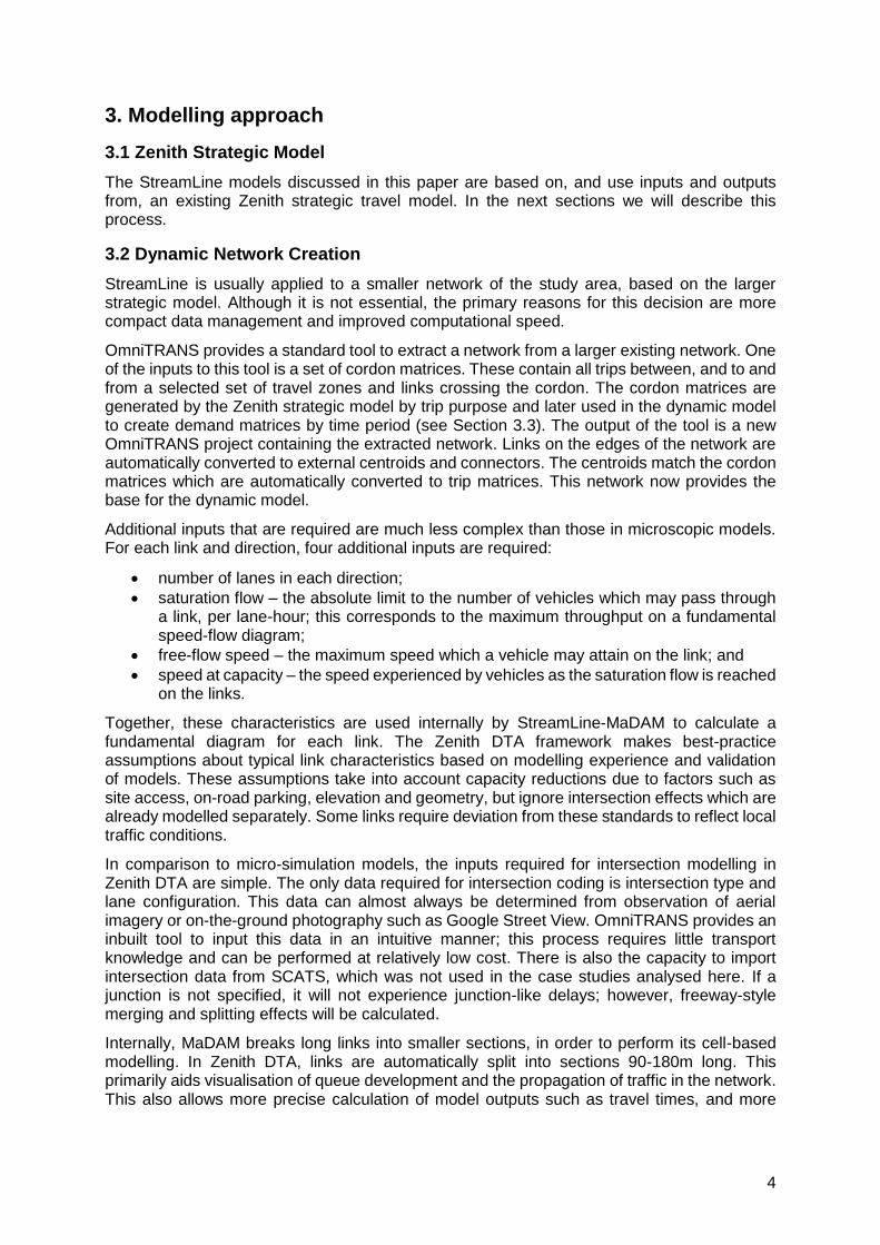
Internally, MaDAM breaks long links into smaller sections, in order to perform its cell-based modelling. In Zenith DTA, links are automatically split into sections 90-180m long. This primarily aids visualisation of queue development and the propagation of traffic in the network. This also allows more precise calculation of model outputs such as travel times, and more


5

precise implementation of traffic controls such as ramp metering. Figure 2 shows an example of this.

Figure 2: Link splitting in Zenith DTA

Original network Network after link splits

3.3 Demand matrix creation

A key characteristic of a dynamic model is the explicit modelling of time. It is therefore necessary to provide the model with detailed information about travel demand at short time intervals.

The base matrices that underpin the dynamic matrices are created in the Zenith strategic travel model. These matrices are constructed by trip purpose, mode and time period. The Zenith strategic travel model calculates travel demand for both two hour peaks and an off-peak. These are then converted into matrices by time interval, using departure time profiles.

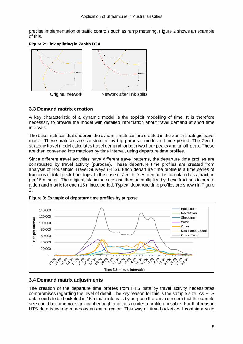
Since different travel activities have different travel patterns, the departure time profiles are constructed by travel activity (purpose). These departure time profiles are created from analysis of Household Travel Surveys (HTS). Each departure time profile is a time series of fractions of total peak-hour trips. In the case of Zenith DTA, demand is calculated as a fraction per 15 minutes. The original, static matrices can then be multiplied by these fractions to create a demand matrix for each 15 minute period. Typical departure time profiles are shown in Figure 3.

Figure 3: Example of departure time profiles by purpose

3.4 Demand matrix adjustments

The creation of the departure time profiles from HTS data by travel activity necessitates compromises regarding the level of detail. The key reason for this is the sample size. As HTS data needs to be bucketed in 15 minute intervals by purpose there is a concern that the sample size could become not significant enough and thus render a profile unusable. For that reason HTS data is averaged across an entire region. This way all time buckets will contain a valid

-

20,000

40,000

60,000

80,000

100,000

120,000

140,000

Tri

ps

per

inte

rval

Time (15 minute intervals)

Education

Recreation

Shopping

Work

Other

Non Home Based

Grand Total

6

number of samples from the HTS, with the drawback that detail for region-to-region travel or by distance buckets is lost.

Whilst the matrices created from these generic departure time profiles provide for a good base for dynamic modelling, it does not necessarily represent the exact demand on any given road in a model. A reason for this could be deviations from average distances as found in the HTS. For example, longer distance trips from outer areas lead to earlier departure times. The same applies when high levels of congestion are expected. This might impact on the reliability of a trip and thus an earlier (or later) departure time might be chosen by the traveller.

For this reason, some matrix estimation techniques have to be applied in order to enrich demand matrices with local travel patterns. Matrix estimation can either be done manually or automatically. We believe the best approach is to initially analyse traffic flows, and if required, manually correct matrices. This way, through traffic engineering skills and local knowledge, the soundness of the adjustment can be assured. Only when the matrices are of a sufficient quality, and the demand is not impacted by congestion, can an automated matrix estimation technique be applied.

Zenith DTA makes extensive use of 15-minute counts in order to calibrate travel demand. Figure 4 shows an example of a single count validation by time period.

Figure 4: Single count validation example (from M1 Managed Motorways case study)

At key locations, such as on motorways and other high-volume roads, the traffic flow profiles are analysed. If required, the profile might have to be adjusted by calibrating the demand matrices for trips passing through that location.

Specific care has to be taken in the analysis as to whether travel demand is impacted by congestion. Instead of removing the demand to match observed data, traffic has to be allowed to queue up- or downstream depending on observed queuing data.

In Zenith DTA the corrections applied to profiles are relatively simple – each is applied using a smooth line or curve (see Figure 51). These adjustments are then applied identically to all demand matrices by trip purpose. Because counts may not respond perfectly to demand matrix changes (particularly in cases where capacity is a limiting factor), several iterations of demand matrix changes may be required.

1 Note that the adjustment in Figure 5 abruptly stops at 8:00 AM, as this is where capacity constraints and queuing begin to dominate the throughput, rather than demand.

0

20

40

60

80

100

120

0

200

400

600

800

1,000

1,200

1,400

1,600

1,800

2,000

Sp

eed

(km

/h)

Veh

icle

s p

er

inte

rval


12A Pacific Motorway (Logan River Bridge) - Northbound

Observed data Modelled

30,729 vehicles (5.8%)

14,054 vehicles (10.2%)AM Peak

29,044 vehicles

12,748 vehicles

Total Period


7

Figure 5: Calibration process at individual count sites

The process of validating the model, calculating a new correction profile for a count site, generating a new cordon matrix and starting a new simulation generally only takes around 15-30 minutes. The order in which count sites are calibrated is at the discretion of the modeller.

Demand matrices used in future year forecasting and/or project case testing are initially generated from the Zenith strategic travel model to ensure wider regional effect to be incorporated in the Zenith DTA model. These matrices are then enriched with the results of the calibration process as explained above using a procedure originally developed in The Netherlands by the Adviesdienst Verkeer en Vervoer (1999b). This procedure examines the differences in the internal structure of the matrices before and after calibration and applies the relative or absolute differences to the future year or project case matrices.

3.5 Run process

StreamLine-MaDAM requires the generation of routes before traffic can be assigned. Zenith DTA models typically use the OmniTRANS OtTraffic class, the default inbuilt static traffic assignment process in OmniTRANS. This is the easiest way to generate route information in OmniTRANS – OtTraffic can take the original static demand matrices, assign this demand to the static network and output the route(s) taken between each origin and destination for later use by MaDAM; in effect, select link assignments can be generated on-the-fly to allow rapid matrix manipulation.

Routes can also be generated in StreamLine by using a Monte Carlo simulation. These can be filtered by a range of criteria to improve processing speed. The results of the Monte Carlo route generation in the two case studies we performed did not improve model validation and were therefore not used. More research is required in order to use the Monte Carlo simulation satisfactorily. A third alternative is the use of route fractions; rather than generating routes between origins and destinations, the turn fractions at every node (usually generated from a static model) are used to route propagating traffic through the network. This method is much less computationally expensive than the other two methods but is generally less precise; therefore, it was not used in either case study.

Once routes are generated, the combination of route set, demand matrices and network are fed to MaDAM and dynamically assigned (the underlying technical details of this assignment are outlined in section 2). Ideally, each model is run for 25-30 iterations. However, usable preliminary results are available after as few as six iterations, which may assist when performing iterative manual calibration.

-50%

-45%

-40%

-35%

-30%

-25%

-20%

-15%

-10%

-5%

0%

-

250

500

750

1,000

1,250

1,500

1,750

2,000

2,250

Ad

jus

tmen

t

Veh

icle

s p

er

inte

rval


Matrix adjustment curve

Count

Input model

Output model

Adjustment

8

3.6 Dynamic traffic control

StreamLine-MaDAM supports the inclusion of control objects, which can be used to interact with the dynamic traffic assignment at specific time intervals, to simulate ramp meters, variable messaging signs and level crossings. Many of these have potential uses in testing incident management on managed motorways, and the response of both motorways and other un-managed roads to crashes and roadworks.

Of particular importance in the M1 Managed Motorways project is ramp metering. MaDAM is capable of dynamically reducing throughput on a given on-ramp based on the upstream flow on the freeway. The only inputs required are activation speeds, and minimum and maximum ramp throughputs. Using such objects, the effects of such ramp metering can be quantified.

4 Case study 1: Wembley Road

4.1 Background

Wembley Road is an arterial road in the south of Brisbane that runs between Kingston Road and Browns Plains Road. It connects Central Logan and the development area of Berrinba with Logan and the wider Brisbane area.

This particular study focuses on the Wembley Road interchange with the Logan Motorway. It aims to assist Transport and Main Roads (TMR) with decisions regarding staging and the assessment of traffic flows in 2021 and 2031, in order to undertake an options analysis and to recommend staged upgrades of Wembley Road and nearby intersections to cater for increased future demand. As part of this project, the traffic impact of key intersections on Wembley Road and the surrounding network (especially the Logan Motorway) was assessed using the Zenith DTA model of Wembley Road.

4.2 Traffic model specification

The model contains Wembley Road and the surrounding area. It is constructed based on the whole of South East Queensland (SEQ) Zenith model. Figure 6 shows the extent of the model. The specifications of the network are shown in Table 1.

Figure 6: Extent of Wembley Road model


9

Table 1: Network characteristics of Wembley Road model

Number of links Number of nodes Junctions

Total Zones Signalled Roundabouts Other

3,508 2,856 256 56 13 54

Some figures on the simulation itself are shown in Table 2.

Table 2: StreamLine simulation characteristics of Wembley Road model

Model year

Timing Number of Route choice moments

Start time End time Output aggregation

Simulation time step

2011, 2021, 2031

05:00 10:00 5 minutes 2 seconds 20

14:00 19:00

Over 120 intersections are defined in the model, of which half are signalised. Specific care is taken for intersections that contain slip lanes. These are manually added in the model (see Section 6.2).

4.3 Calibration and validation

A large collection of counts and travel times were available for validation purposes. The model was manually calibrated at specific locations where a clear difference from observed data was evident. In particular, longer trips from outside Brisbane tend to depart earlier than the general departure time profiles suggest. This localised behaviour needed to be dealt with manually by the modeller because of the specific nature of the traffic demand. Matrix Estimation was used for the remainder of the counts that were not affected by congestion to ensure correct local demand on the intersections and connecting links. Figure 7 shows a high level of correlation between the modelled and observed volumes in the morning peak.

Figure 7: Validation results of Wembley Road model, morning peak

4.4 Modelling

The model identified locations outside the direct study area where the provided infrastructure will be deficient in the future years. In consultation with the client, these locations were upgraded in the model so as to not disturb traffic flows entering the study area.

y = 0.9763xR² = 0.9926

0

2,000

4,000

6,000

8,000

10,000

12,000

14,000

16,000

0 2,000 4,000 6,000 8,000 10,000 12,000 14,000 16,000

Mo

de

lled

vo

lum

e

Observed volume

Observed vs Modelled volumes 5.30-10am

10

A number of staging options for the Wembley Road interchange with the Logan Motorway were identified by the client and tested in the dynamic model at each future year horizon. A number of performance indicators were then extracted from the model to assess the performance of each of the options. These include:

Travel times on key routes though the study area

Average delay on intersections

Queue lengths

Average speed of the network

Throughput of network

Level of service

The XStream module provides outputs on intersections which are useful for higher level analysis like delay, back of queue, spare capacity, and volume over capacity ratios. It can neither deal with coordinated intersections nor provide outputs required for detailed operational analysis. Therefore the intersection analysis tool SIDRA INTERSECTION was used to undertake more detailed analysis of the performance of intersections.

4.5 Results

Around 15 upgrades were recommended including suggested staging of options for road and intersection configurations. The first stage of this project has been delivered as part of ten year horizon projects for TMR.

5 Case study 2: M1 Managed Motorways

5.1 Background

The Pacific Motorway (M1) is a key freeway in South East Queensland. At its southern end, it is the only freeway-grade connection between Queensland and New South Wales. With its connection to the Gateway Motorway, it also forms one part of a continuous stretch of motorway between New South Wales and the Sunshine Coast. It also forms an important commuter route, connecting the Gold Coast and Logan areas to the Brisbane CBD.

The model is more complex than the Wembley Road project, owing to the increased size of the study area. It extends from Eight Mile Plains in the north to the Nerang River in the south, following the path of the M1. It also includes large portions of the surrounding local and arterial road network, in an effort to correctly model alternative routes to the motorway. It also includes portions of the Logan Motorway and Gateway Motorway.

The model is an on-going internal research project to assess the impact of managed motorways projects on a high-volume motorway in Brisbane. Ramp metering was implemented using StreamLine control objects (see Section 4.1.5). This allowed for the modelling of ramp metering not just as it is currently implemented on the Pacific Motorway, but also assuming alternative and future-year scenarios. Other aspects of managed motorways, such as incident and speed management, are also implementable in this model.

5.2 Traffic model specification

The model is constructed based on the whole of SEQ Zenith model. Figure 8 shows the extent of the model in red. The specifications of the network are shown in Table 3, and the simulation parameters are show in Table 4.


11

Figure 8: M1 Managed Motorways model area

Table 3: Network characteristics of M1 model

Number of links Number of nodes Junctions

Total Zones Signalled Roundabouts Other

10,865 9,924 533 187 81 267

Table 4: StreamLine simulation characteristics of M1 model

Model year

Timing Number of Route choice moments

Start time End time Output aggregation

Simulation time step

2013 04:00 10:00

5 minutes 2 seconds 1 14:00 19:00

5.3 Calibration and validation

The calibration process for this model presented the opportunity to significantly improve the original validation. Using the general departure time profiles did not result in traffic flows reflecting actual conditions along the M1 corridor. Traffic volumes on the motorway are generally much more uniform and do not show much of a peak pattern. As a result, even though most count sites validated reasonably well across the two-hour peak periods, they were not as accurate across the entire simulation period. This necessitated local adjustments to the demand matrices in order to correctly model traffic flows on the network. Count sites were generally calibrated in the direction of travel, so that a large proportion of the traffic flowing through each count site was already correctly calibrated based on the previous count site.

Due to the size of the network, slow traffic propagation also posed a problem. Because StreamLine starts with an initially empty network, traffic from the far edges of the model did not reach their destinations in time to contribute to the observed level of congestion. As a result,

12

congestion in the early modelled period was too low. The solution to this problem was to begin the simulation an hour earlier but to end at the same time, extending the total simulation period by an hour. This caused some increase in running times, but had a net positive effect on calibration of the model.

While it is important to note that this model is still a work-in-progress, some preliminary validation results are presented in Figure 9 below.

Figure 9: Validation results M1 DTA model, morning peak

Although the r-squared value is not as high as desired (improvements are still being made to the model), it still shows a high correlation between count and modelled volumes.

5.5 Results

The calibrated model was capable of testing a variety of scenarios. The most important to the original purpose was the testing of the effectiveness of ramp metering. Currently, ramp meters operate on four of the northbound (inbound) on-ramps within the model area – at Logan Road (Upper Mount Gravatt), Sports Drive, Paradise Road and Loganlea Road. The base calibrated model includes these on-ramps, using the same parameters as those used in reality.

One test was performed in which these ramp meters were removed from the base year 2013 model, to determine their effect on the network as a whole. Some key metrics of the two results are summarised in Table 5. Note that for the purposes of this comparison, queuing is defined as the time during which any part of the northern section of the M1 (from the Logan River to the Gateway Motorway) experiences a speed less than 50% of the free-flow speed.

Table 5: Comparison of ramp metering tests in M1 Managed Motorways model

Ramp metering

Average Travel Time (mm:ss) Maximum Travel Time (mm:ss) Maximum length of

queue (km) Logan River-Underwood Rd

Underwood Rd-Gateway Mwy

Logan River-Underwood Rd

Underwood Rd-Gateway Mwy

With 17:17 01:01 40:22 01:02 13.9

Without 20:29 00:59 49:07 01:01 21.1

The results confirm the effectiveness of the ramp meters in these locations, with overall traffic throughput and average speed much higher with ramp meters implemented. The effect is further demonstrated in Figure 10, which compares flow on the M1 just south of a metered on-ramp (Sports Drive) with and without the inclusion of ramp meters. The ramp metered scenario

y = 0.9911xR² = 0.9583

0

5,000

10,000

15,000

20,000

25,000

0 5,000 10,000 15,000 20,000 25,000

Mo

de

lled

Vo

lum

e

Count Volume

Observed vs Modelled Volumes 6-9am


13

clearly demonstrates an increase in overall throughput; the scenario without ramp metering only rises towards the end of the simulation period, once volume on the on-ramp itself has begin to reduce.

Figure 10: Comparison of ramp metered and non-ramp metered models

These results can also be visualised by way of a space-time diagram, which shows modelled travel speeds (relative to the freeflow speed) by time and distance along a corridor. Figure 11 below demonstrates the differing speed patterns when comparing ramp metered and non-ramp metered models.

Figure 11: Comparison of ramp metered and non-ramp metered models

This graphical comparison gives users a more intuitive understanding of the effects of the ramp metering; without its implementation, congestion persists for a longer time, queues form over greater distances, and speeds achieved through the congested area are generally lower than in the scenario with ramp metering.

0

50

100

150

200

250

300

350

400

Th

rou

gh

pu

t (v

eh

icle

s p

er

5 m

inu

tes)

Time

Comparison of ramp metered and non-ramp metered models

Meter active

With

Without

14

6. Adaptation for the Australian market

Because of its origins, StreamLine is somewhat geared to a European situation. We have found that a couple of adaptations are necessary in order for StreamLine to be fully usable in the Australian market.

6.1 Merging and weaving

On high-volume freeway merges, StreamLine-MaDAM tends to be fairly aggressive in its assumptions of capacity reduction due to merging. As a result, assigned speeds will drop below those typically experienced in reality. Saturation flows around these merge locations may be increased in these circumstances on a case-by-case basis. One example from the M1 Managed Motorways project is the merging from four lanes to three on the M1 immediately after the off-ramp to the Logan Motorway. This location generally does not cause much congestion, as drivers have plenty of room to merge and may tend to avoid the two merging lanes. Therefore, the saturation flow at this merge was increased to 2600 veh/h/lane, a figure which is also used at other problematic merges.2

The particular lane configurations upstream of a split may also induce weaving, which must be modelled in MaDAM by reducing saturation flows. Again from the M1 Managed Motorways project, an example is the off-ramp from the M1 to the Gateway Motorway. Here, drivers in the left two lanes must move to the right two lanes if they wish to continue towards the Brisbane CBD. Saturation flow in this area was thus reduced to 1750 veh/h/lane to induce the speed reductions usually seen in the peak period.

6.2 Junctions

Perhaps unique to Australian uses of StreamLine is the modelling of slip lanes at intersections (see Figure 12). As they are not, by default, specifiable in OmniTRANS’ junction editor, they must be modelled separately: they are added as entirely separate links. Left turns are then banned through the intersection itself, so all left-turning traffic must use a slip lane if available. This allows left-turning traffic to avoid some of the same delays that would be experienced through the nearby junction, unless vehicles cannot reach the slip lane due to queuing. They also avoid contributing to turn delays through the intersection.

Figure 12: Coding of junction with left turn slip-lanes in StreamLine

Links and nodes (with slip lanes) Junction

2 While saturation flow was used to reduce congestion in the case studies presented here, it may also be possible to achieve the same effect by modifying the underlying MaDAM parameters, especially when the effect is less localised. This possibility is currently under investigation.


15

7. Conclusions

The two case studies that are discussed in this paper prove that StreamLine can be successfully applied in the Australian market. The Zenith DTA model offers a complete range of outputs suitable for detailed analysis. It has also proven to be a cost-effective tool since a strategic transport model can provide the underlying networks and demand matrices. Additional inputs in the form of dynamic attributes and intersection details are required, however some of these can be automated and manual inputs are supported by an effective graphical user interface. We found that the biggest cost factor is in calibrating the model to reflect actual traffic conditions. This needs to be a manual process so that the modeller stays in full control of the adjustments. Only when a suitable level of calibration is achieved may matrix estimation be applied. This process means that a number of adjustments and subsequent modelling iterations are required.

References

Adviesdienst Verkeer en Vervoer 1999b, Gebruikershandleiding RGM, rapportnummer AVV/Fok/6767, Adviesdienst Verkeer en Vervoer, Rotterdam, The Netherlands

Bellemans, T, De Schutter, T, De Moor, T (2002) Models for traffic control, Journal A, vol. 43, no. 3–4, 13–22.

Daganzo, C F (1994a) The Cell Transmission Model: A Dynamic Representation of Highway Traffic, Consistent with Hydrodynamic Theory, Transportation Research Board 28(4), 269-287.

Daganzo, C F (1994b) The Cell Transmission Model, Part II: Network Traffic. Transportation Research, B 28(2), 279-93.

Dijkhuis, N (2012) ‘Dynamic user equilibria in StreamLine’, Master thesis, University of Twente, Enschede.

Transportation Research Board (2000) Highway Capacity Manual, Transportation Research Board, Washington, D.C.

Hoogendoorn, S P, Bovy, P H L (2001) State-of-the-art of Vehicular Traffic Flow Modelling Special Issue on Road Traffic Modelling and Control of the Journal of Systems and Control Engineering, Delft, The Netherlands.

Lighthill, M H, Whitham, G B (1955) On kinematic waves II: a theory of traffic flow on long, crowded roads. Proceedings of the Royal Society of London series A, 229, 317-345.

Messmer A., Papageorgiou M., 1990. METANET: a macroscopic simulation program for motorway networks, Traffic Engineering and Control, 31, p466–470.

Raadsen, M P H, Mein, H E, Schilpzand, M P and Brandt, F (2010) Applying StreamLine DTA model on the Amsterdam beltway, Contribution to the Colloquium Vervoersplanologisch Speurwerk, Roermond, The Netherlands.

Richards P, (1956) Shock waves on the highway, Operations Research 4, p42-51.

Veitch Lister Consulting 2014, Zenith Dynamic Traffic Assignment Model of Wembley Road, Veitch Lister Consulting, Brisbane.

application of streamline in australian cities -...

Documents