application of response surface methodology for …jestec.taylors.edu.my/vol 15 issue 1 february...

Journal of Engineering Science and Technology Vol. 15, No. 1 (2020) 655 - 674 © School of Engineering, Taylor’s University

655

APPLICATION OF RESPONSE SURFACE METHODOLOGY FOR THE OPTIMIZATION OF THE CONTROL FACTORS

OF ABRASIVE FLOW MACHINING OF MULTIPLE HOLES IN ZINC AND AL/SICP MMC WIRES

MOHAMMED YUNUS1,*, MOHAMMAD S. ALSOUFI1

1College of Engineering and Islamic Architecture, Umm Al-Qura University, Al-Abdiah, Makkah, Kingdom of Saudi Arabia *Corresponding Author: [email protected]

Abstract

In the present age of adopting non-conventional finishing techniques, it is high time to apply these methods for micromachining of multiple holes in hardware components such as wires made of metals and composite materials to make them successful trends were hard to complete with finishing. Abrasive flow machining has the potential to use one of the advanced finishing techniques in the aerospace, medical and automotive fields. Current work focuses on optimizing the input parameters of micro-machining of multiple holes in a wire made of zinc and Al/SiCp composite materials with a high percentage of Silicon Carbide particles machined using abrasive flow jet with the multi-objective of minimizing surface roughness, Ra, and maximizing machining removal rate (MRR). Using input parameters such as pump pressure, abrasive mesh size and concentration, number of cycles and oil concentration percentage, the experiments were conducted according to a Taguchi L27 orthogonal array. ANOVA predicted the relative importance of input parameters and their contribution level. In addition to this, mathematical models for establishing a relationship between input parameters and machining characteristics were also developed. The pump pressure was the highly influential factor affecting the Ra and MRR. The Box-Behnken design of response surface methodology is applied with a desirability function approach to determine the optimum set of parameters for minimizing Ra and maximizing the MRR. The advanced technique shows flexibility based on the product application could be tested and established.

Keywords: Machine removal rate, Optimization, Orthogonal arrays, Response surface methodology, Surface roughness.

656 M. Yunus and M. S. Alsoufi

Journal of Engineering Science and Technology February 2020, Vol. 15(1)

1. Introduction Abrasive flow machining (AFM) is a futuristic production technique to develop the products of high-quality surfaces concerning areas difficult to reach such as inner sections, cross holes, internal passages, micro-sized holes and slots, concave and convex edge blending, and others [1]. Deburring, removal of recast layers and radial surfaces and polishing of the above features are complicated, and in achieving these manually, there is a risk of damaging the other finished surfaces.

This may cause a significant loss such as an engine’s energy loss, failure of aero-engines parts, faults in devices, and so on. Industries have been trying hard with considerable investments in finishing of these components to remove burrs and scratch marks on the components. For a few decades, the traditional manufacturing type of finishing methods (grinding, lapping and honing, and so on) has been used to perform finishing on the machined parts. Recently, it is found that entrapment of hidden loose metal particles on the seating surfaces of many components through cross-holes or inner passages does not allow full control on parts and can only be seen with higher magnification. It becomes difficult to remove such particles and to finish in the shop floor, as all types of equipment are not generally made available [2, 3]. In such instances, AFM could be useful for high quality deburring, polishing and rounding of edges on internal and external surfaces of machined components by using an abrasive loaded polymer flowing forcibly into the controlled channel employing hydraulic pressure. In restricted channels, the abrasive particles come into maximum cutting action to perform deburring and rounding of edges as well as polishing. The abrasive medium is either allowed to flow in the upward or downward direction to improve the material removal rate (MRR) and surface finish (Ra). An abrasive medium is composed of a type of abrasive particles for finishing, the polymer for carrying abrasive and oil to control the viscosity.

The abrasive medium requires appropriate fluidity for passing into restricted slots/holes. Tooling is another part of the AFM process to guide the medium regarding were to perform finishing within the slot or hole, the next target point and is designed to perform finishing in either one passage or the number of passage courses. As it comes in direct contact with the tool, professionally all non- homogeneous materials such as non-ferrous alloys, superalloys, ceramics, carbides, semiconductors, quartz, composites and so on, which are not compatible with the traditional manufacturing methods; become possible by the AFM. It is known that good surface finished metals and composite materials have broad applications. Extrude-Hone Corporation of the USA developed the AFM concept for finishing of aero-engine parts to a higher accuracy level in 1960. At present, AFM is recognized for finishing and polishing of intricate geometries not approachable by the traditional methods [4, 5].

The fact that AFM exhibits a higher material removal rate (MRR) for soft materials have been reported. A full factorial statistical method was adopted for investigating the effect of cutting force and current grain density using input variables such as extrusion pressure, abrasive concentration and grain size on surface roughness (Ra) [6]. A response model was developed using a surface methodology (RSM) for AFM to find the effect of control variables on the Ra of titanium alloy 6Al4V [7]. The indicate shapes are usually cut by wire EDM method subjected to finishing by AFM. Magnetic type AFM process was designed for

Application of Response Surface Methodology for the Optimization . . . . 657


accomplishing high MRR and improved surfaces [8]. AFM improved the surface roughness by supplying coolant and concentration of abrasive powder [9]. Ko et al. [10] mentioned a finite element analysis (FEA) illustration was presented to investigate the potential magnetic distribution in the magnetic abrasive flow polishing process. An FEA model was prepared to take the effect of the media flow rate in AFM successfully.

According to Wani et al. [11], results of the varying magnetic field by applying it on magnetic and nonmagnetic specimens in the magneto-rheological abrasive honing process were presented and showed the magnetic field near the non-magnetic specimens was increased. The rotary AFM process has been developed for finishing technique with intention of maximizing the MRR and minimizing the Ra and produced a result of 44% decrease in Ra and 83% increase in MRR compared to a conventional AFM method [12].

Vibration-assisted cylindrical magnetic abrasive finishing process on aluminium workpiece was investigated experimentally to maximize MRR [13]. The relationship between input and response parameters in AFM process was investigated experimentally to discover the system of MRR in Nano finishing of metal matrix composites (MMCs). It showed that the particles are randomly distributed in MMCs [14]. It is a major task to finish hard and heterogeneous materials, (i.e., MMCs). Such hard materials are required to be cut by methods like EDM and then finished by processes like AFM.

For achieving a good surface finish, some cycles are required as work material gets harder. Optimization of the input parameters such as abrasive particle size, abrasive concentration, extrusion pressure and machining time of AFM using the Taguchi method was carried out and investigated the optimum solutions affecting the machining quality [15]. Based on studies by Mulik and Pandey [16], the ultrasonic-assisted magnetic abrasive finishing process was investigated experimentally to compare it with the conventional AFM process. A mathematical model was obtained for investigating the applied force and torque to forecast Ra using RSM with Box-Cox transformation in turning operation of AISI 1019 steel [17]. The effect of input parameters on Ra has been studied and shown that the feed is a majorly affecting factor.

Jain and Jain [18] proposed that the neural network (NN) for modelling and optimal range of input parameters of the AFM process produced results, which have been validated; with optimization results of the AFM method obtained using a genetic technique. The optimization of surface texture response has shown that the input parameters like the cutting speed, the tangential second relief angle were most influencing factors [19]. The rheological characteristics of materials for the description of AFM process and developing the relationship with the process were studied so far has been reported on materials like brass, aluminium, steel, and so on [5, 20, 21].

In recent studies by Jain and Jain [22], determining an optimal set of process parameters to obtain response characteristics has become the principal concern of several researchers. In this work, Zinc and MMC wires were taken up because of their realistic and live engineering parts widely used in the hardware industry. Also, to study the viability of integration of this alluring technique (i.e., AFM) with the present small-scale industries [23].



Thus, makes it more appropriate, cost-effective, and feasible for common applications and to cut on the manufacturing costs in preparing them. Zinc wire for single output optimization was studied but not for multi-output optimization, and in case of a metal matrix composite (MMC) Al/SiCp having Al base material reinforced with a high percentage of hard material particles (SiCp) are not studied for single as well as multi-output optimization has led to take up this work Hard material composite and base metal wires are finished by AFM and have broad applications in the industry to continually improve the performance of the AFM process. Hiremath et al. [24] reported that the goal of this work is to investigate the optimal set conditions of the chosen control parameters to reduce Ra value and to increase metal removal rate using RSM design methodology in AFM.

2. Materials and Methods From the literature review, five control or input factors were chosen for the present study to limit the volume of work and to follow the straight path approach for some of the input parameters involved in the experimental investigation as listed in Table 1. The possible process parameters, which influence the potential efficiency of the method and the ensuing quality of parts finished by AFM are selected based on three major parts of the process namely machine (extrusion/pump pressure and total amount of cycles), medium (abrasive size, concentration and % in oil concentration) and workpiece (material). Omitted parameters indirectly are indicators or presenters of chosen parameters. For example, the media flow rate depends on pump pressure for a given sample and similarly the media flow quantity described by some cycles for given machine setup, viscosity depends on percentage oil concentration and others. Material removal rate (MRR) and change in Ra are selected as responses indicating the performance measures of the AFM method.

Table 1. Important factors and their levels.

Process parameters Unit Designation Level 1 2 3

Pump pressure bar A 10 25 35 Abrasive concentration % B 50 60 70 Abrasive mesh size µm C 150 225 300 Number of cycles - D 15 30 45 Oil concentration % E 5 10 15 Workpiece material - F Zinc Al/SiCp -

2.1. Experimental methodology The sample’s initial weight was measured, and its length cut into two equal portions by the EDM-wire-cut method to measure the initial surface roughness, Ra by taking an average of different spots in the central region of every hole before finishing. To measure the Ra value, the media flow direction was selected using a particular die prepared for clamping at the sections of the two parts of samples, i.e., pin cylinder lock bodies are mounted on the AFM set up to carry out finishing process at the machining set conditions. An accurate electronic balancing machine with accuracy up to 10-4 grams was employed to assess the sample’s weight.

The samples were removed from the AFM unit using the uniquely designed die for gripping together the two components of samples and were well cleaned with



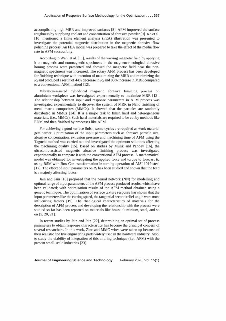
acetone solution to prepare for conducting measurements (refer Fig. 1). Both parts of samples (pin cylinder lock bodies) were weighed to measure final weight. Similarly, the final Ra value is measured at various spots of a central region of every sample’s hole after finishing and averaged. The MRR quantity was measured by computing the variation between the average initial and final weight of the samples in a stipulated time of finishing by AFM under the standard set of experimental conditions. The Ra was obtained by measuring the variation between the average Ra values of before and after finishing [25].

The viscoelasticity medium is formulated using silicon-carbide (silicon-based polymer) sharp particles of exact mesh size mixed for the required fraction to maintain their correct percentage by weight. Grease and SAE40 oil have been selected as the abrasive carrier medium in the present investigations. The medium must run 20 to 28 cycles on the trial specimen to obtain a uniform mixture before starting experimentation.

The media used during each run should maintain the proportionate number of new particles having sharp edges. A large amount of media should be prepared and changed after a certain number of cycles to maintain constant output values. Workpiece surfaces consisting of pin cylinder lock bodies possessing several holes with zinc and Al/SiCp MMC were used as work material.

Fig. 1. Experimental setup of AFM

(courtesy of shodhganga.infibnet.ac.in).

Designing series of experiments Experiments are conducted by varying the A to E factors as shown in Table 2. Using the input parameters of mixed levels and the output responses that are considered for the optimization resulted in L27 orthogonal array or twenty-seven runs to achieve a second-order polynomial regression [9, 26, 27].



Table 2. Experimental results as per L27 orthogonal array.

Run no.

Pump pressure

Concentration of abrasives

Abrasive mesh

number

Number of cycles

Percentage of oil in media

Ra for Al/SiCp

Ra for Zn

MRR for

Al/SiCp

MRR for Zn

1 10 50 150 15 5 0.0045 0.0047 0.0001 0.0001 2 10 50 150 15 10 0.0205 0.0213 0.0015 0.0016 3 10 50 150 15 15 0.0470 0.0489 0.0219 0.0937 4 10 60 225 30 5 0.0320 0.0307 0.0039 0.0040 5 10 60 225 30 10 0.0845 0.0812 0.0620 0.0645 6 10 60 225 30 15 0.0105 0.0109 0.00050 0.0005 7 10 70 300 45 5 0.1023 0.1064 0.09025 0.0939 8 10 70 300 45 10 0.0143 0.0148 0.0011 0.0012 9 10 70 300 45 15 0.0606 0.0631 0.0369 0.0384

10 25 50 225 45 10 0.1481 0.1541 0.1190 0.1238 11 25 50 225 45 15 0.2248 0.2337 0.1905 0.1981 12 25 50 225 45 5 0.0270 0.0281 0.0023 0.0023 13 25 60 300 15 10 0.2769 0.2880 0.2253 0.2343 14 25 60 300 15 15 0.0342 0.0382 0.0065 0.0068 15 25 60 300 15 5 0.1743 0.1812 0.1383 0.1438 16 25 70 150 30 10 0.0385 0.0401 0.0100 0.0104 17 25 70 150 30 15 0.1983 0.2062 0.1681 0.1749 18 25 70 150 30 5 0.3706 0.3855 0.2958 0.3076 19 35 50 300 30 15 0.4055 0.4217 0.3143 0.3268 20 35 50 300 30 5 0.0433 0.0450 0.0128 0.0133 21 35 50 300 30 10 0.2510 0.2610 0.2108 0.2192 22 35 60 150 45 15 0.0705 0.0733 0.0503 0.0523 23 35 60 150 45 5 0.3140 0.3266 0.2530 0.2631 24 35 60 150 45 10 0.4345 0.4519 0.3356 0.3491 25 35 70 225 15 15 0.3428 0.3565 0.2848 0.2961 26 35 70 225 15 5 0.4603 0.4787 0.3518 0.3658 27 35 70 225 15 10 0.1270 0.1321 0.1018 0.1058

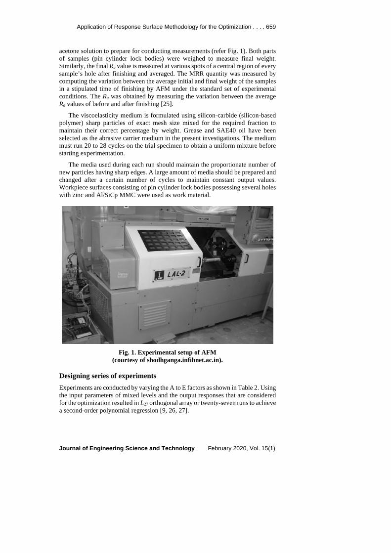
2.2. Response surface methodology (RSM) The RSM is an optimization technique to locate the optimum set of variables, which are unknown before running the experiment. Hence, it provides a design to obtain the equal precision of estimation in all directions. The application of RSM based design optimization is designed for avoiding the expensive analysis methods (e.g., Finite Element Analysis, CFD) and their associated numerical noise [28]. RSM is used for the modelling and analysis of engineering problems with the primary objective to optimize input variables influencing the responses and quantifying the relationship between them. The steps involved in RSM are as follows as shown in Fig. 2.



Fig. 2. Steps involved in RSM optimization.

Box-Behnken design (BBD)

RSM designs allow estimating the interaction of variables and even their quadratic effects. Box-Behnken methods are well-organized designs for fitting the 2nd order polynomials to output surfaces, as they use a reasonably few number of observations to assess the factors. BBDs are formed by combining 2k factorials with incomplete block designs. The BBD method does not contain points at the vertices of the cubic volume produced by the upper and lower limits of each factor.

3. Results and Discussion The study is carried out to optimize the control parameters of AFM with RSM using Box - Behnken design for the two different workpieces made of a metallic and composite material. Decisions should be taken pertaining to parameters, which influence the performance of a process. The loss functions insist on design parameters, which influence the typical and variation of a process output characteristic of a product or process.

By appropriately adjusting an average and decreasing disparities, the losses can be reduced. Intended changes to one or more factors are made to monitor the effect that those changes have on one or more performance parameters (responses). Design of experiments is a well-organized method for planning experimental runs so that the data is scrutinized to yield convincing and useful conclusions. The analysis of variance (ANOVA) method must be applied to understand the impact of various input parameters and their interactions on the responses and the fitness of the developed model.

3.1. Effect of AFM input parameters The experiments were conducted to investigate the cause of AFM input factors on responses of AFM such as MRR and Ra and optimum condition of input variables was found out using ANOVA. The significance and percentage contribution of each variable along with the confidence level and the variance of the data is expressed in Tables 3 and 4. The Model F-value indicates the



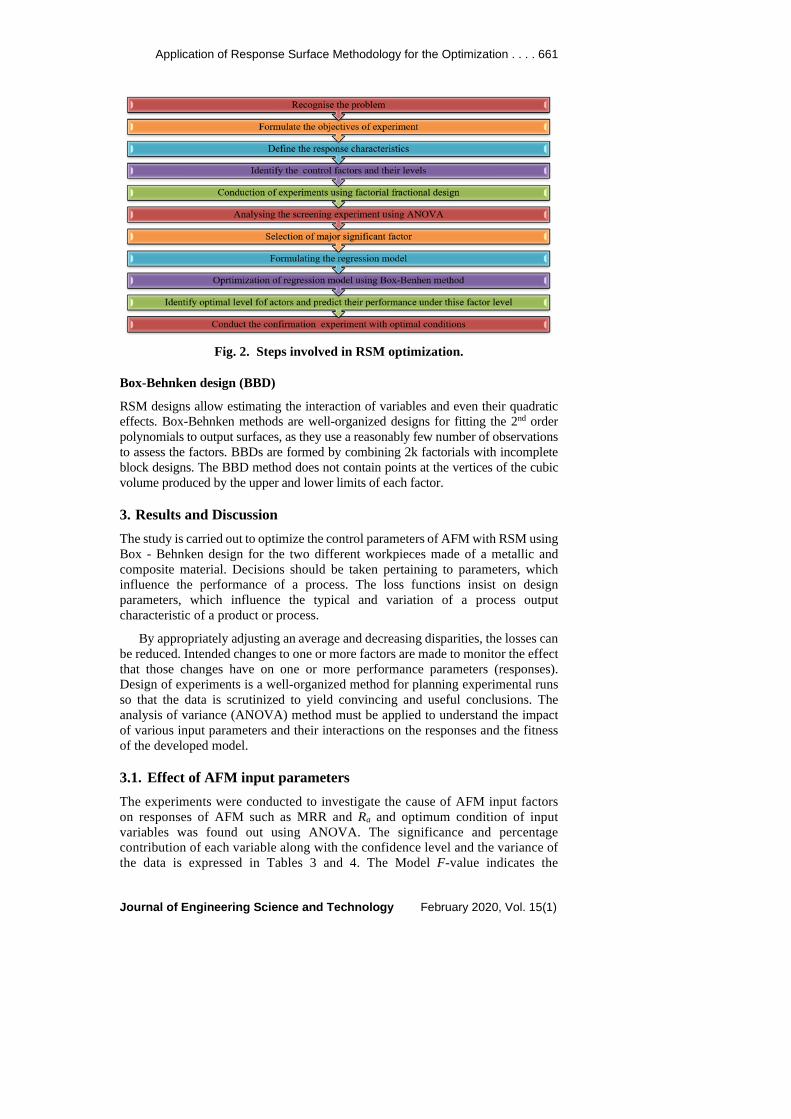
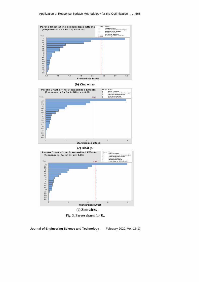
importance of the model, which has the only chance of 0.0103% for F-value to be larger due to noise. The Fisher F-test with a probability value as low as 0.05 demonstrates the significance of the model terms. The data formulated a correlation model between the output and the independent input parameters. The higher F value in ANOVA, the critical parameter “A” is highly significant when individual and 2-way interaction levels (squared) compared to all other factors for all the responses as depicted in Pareto diagrams (refer Fig. 3). Hence, parameter A holds major significance role for all responses.

Table 3. ANOVA results of surface roughness in Zn and Al/SiCp MMC. ANOVA for response surface quadratic model

Analysis of variance table (partial sum of squares-Type III) Ra for Al/SiCp Ra for Zn

Source DF Adj SS Adj MS F-Value P-Value Adj SS Adj MS F-Value P-Value A 1 0.2387 0.239 15.52 0.006 0.26035 0.2604 15.78 0.005 B 1 0.0164 0.0164 1.06 0.337 0.01771 0.0177 1.07 0.335 C 1 0.0011 1e-3 0.07 0.803 0.00107 0.0011 0.07 0.806 D 1 5e-4 5e-4 0.03 0.867 0.00053 5.3e-4 0.03 0.863 F 1 0.0011 1e-3 0.07 0.804 0.00107 0.0011 0.06 0.807 E 1 1.6e-3 0.0016 0.10 0.761 0.00151 0.0015 0.09 0.771 Square 6 6e-4 9e-5 0.01 1.000 0.00073 1.2e-4 0.01 1.000 A×A 1 5e-4 5e-4 0.03 0.865 0.00061 6.1e-4 0.04 0.853 B×B 1 1e-5 1e-5 0.00 0.980 0.00003 3e-5 0.00 0.969 C×C 1 5e-5 5e-5 0.00 0.955 0.00002 2e-5 0.00 0.972 D×D 1 4e-6 1e-5 0.00 0.987 0.00003 3e-5 0.00 0.970 E×E 1 1.3e-6 1e-5 0.00 0.978 0.00004 4e-5 0.00 0.963 F×F 1 9e-6 1e-5 0.00 0.982 0.00002 2e-5 0.00 0.973 2-way interaction

7 0.1947 0.0278 1.81 0.226 0.21031 0.0301 1.82 0.224

A×E 1 0.0007 0.0007 0.04 0.839 0.00065 0.0007 0.04 0.848 A×F 1 0.0006 0.0006 0.04 0.853 0.000541 0.0006 0.03 0.861

B×E 1 0.073 0.073 4.75 0.066 0.07861 0.0786 4.76 0.065 B×F 1 0.014 0.014 0.91 0.372 0.01491 0.0149 0.90 0.373 C×E 1 0.0061 0.0061 0.40 0.549 0.00638 0.0064 0.39 0.554 C×F 1 0.0037 0.0037 0.24 0.637 0.00409 0.0041 0.25 0.634 D×F 1 0.0594 0.0594 3.86 0.090 0.06377 0.06377 3.86 0.090 Error 7 0.1077 0.0154 0.11551 0.0165 Total 26 0.5615 0.60841

R2 = 98.182% R2 = 98.13% R2 (adj) = 52.65 R2 (adj) = 51.42 R2 (pred) = 0.00 R2 (pred) = 0.00



Table 4. ANOVA results of surface roughness in Zn and Al/SiCp MMC. ANOVA for response surface quadratic model

Analysis of variance table (partial sum of squares-Type III) MRR for Al/SiCp MRR for Zn

Source DF Adj SS Adj MS F-Value P-Value Adj SS Adj MS F-Value P-Value A 1 0.16 0.16 12.8 0.01 0.15936 0.15936 11.7 0.01

B 1 0.0122 0.0122 0.97 0.36 0.0096 0.0096 0.70 0.43

C 1 0.0006 0.0006 0.04 0.84 0.00171 0.00171 0.13 0.74

D 1 0.0002 0.00016 0.01 0.92 0.0009 0.0009 0.06 0.81

F 1 0.0008 0.00076 0.06 0.81 0.00082 0.00082 0.06 0.81

E 1 0.0004 0.00038 0.03 0.87 0.00007 0.00007 0.01 0.95

Square 6 8.2e-4 0.00014 0.01 1.00 0.00143 0.00024 0.02 1.00

A×A 1 5.9e-4 0.00059 0.05 0.84 0.00024 0.00024 0.02 0.9

B×B 1 7e-5 0.00007 0.01 0.94 0.0004 0.00034 0.03 0.88

C×C 1 7e-5 0.00007 0.01 0.94 1e-6 1e-6 0.00 0.99

D×D 1 6e-5 0.00006 0.00 0.95 0.0003 0.0003 0.02 0.89

E×E 1 1e-5 0.00001 0.00 0.98 0.0005 0.00041 0.03 0.87

F×F 1 3e-5 0.00003 0.00 0.96 0.0002 0.00019 0.01 0.91

2-way interaction

7 0.1254 0.01791 1.44 0.32 0.139 0.01985 1.46 0.32

A×F 1 0.0001 0.0001 0.01 0.93 0.00011 0.00011 0.01 0.93

A×E 1 0.0008 0.00079 0.06 0.81 0.00016 0.00016 0.01 0.92

B×E 1 0.0096 0.00957 0.77 0.41 0.00737 0.00737 0.54 0.49

B×F 1 0.0477 0.04768 3.83 0.09 0.0516 0.05157 3.79 0.09

C×E 1 0.0024 0.0024 0.19 0.67 0.00447 0.00447 0.33 0.59

C×F 1 0.00449 0.004489 0.36 0.57 0.00486 0.00486 0.36 0.569

D×F 1 0.03807 0.038066 3.05 0.13 0.0365 0.03651 2.68 0.146

Error 7 0.0873 0.012466 0.09533 0.01362

Total 26 0.3872 0.40884

R2 = 98.182% R2 = 98.13% R2 (adj) = 52.65 R2 (adj) = 51.42 R2 (pred) = 0.00 R2 (pred) = 0.00

The regression models are correlations or mathematical models to forecast each response of the AFM process as a function of input variables. The quadratic relations for the coded levels of the parameters are presented four of the responses in Eqs. (1) to (4) respectively.

∆𝑹𝑹𝐚𝐚 𝐟𝐟𝐟𝐟𝐟𝐟 𝐀𝐀𝐀𝐀/𝐒𝐒𝐒𝐒𝐒𝐒𝐒𝐒 = −𝟎𝟎.𝟐𝟐𝟎𝟎𝟐𝟐 + 𝟎𝟎.𝟏𝟏𝟏𝟏𝟏𝟏 𝑨𝑨 + 𝟎𝟎.𝟏𝟏𝟏𝟏𝟐𝟐 𝑩𝑩 + 𝟎𝟎.𝟏𝟏𝟐𝟐𝟐𝟐 𝑪𝑪 − 𝟎𝟎.𝟐𝟐𝟐𝟐𝟐𝟐 𝑫𝑫− 𝟎𝟎.𝟐𝟐𝟐𝟐𝟏𝟏 𝑭𝑭 + 𝟎𝟎.𝟐𝟐𝟐𝟐𝟏𝟏 𝑬𝑬− 𝟎𝟎.𝟎𝟎𝟎𝟎𝟐𝟐𝟏𝟏 𝑨𝑨 ∗ 𝑨𝑨 + 𝟎𝟎.𝟎𝟎𝟎𝟎𝟏𝟏𝟐𝟐 𝑩𝑩 ∗ 𝑩𝑩 − 𝟎𝟎.𝟎𝟎𝟎𝟎𝟐𝟐𝟎𝟎 𝑪𝑪 ∗ 𝑪𝑪 + 𝟎𝟎.𝟎𝟎𝟎𝟎𝟎𝟎𝟐𝟐 𝑫𝑫 ∗ 𝑫𝑫 + 𝟎𝟎.𝟎𝟎𝟎𝟎𝟏𝟏𝟏𝟏 𝑭𝑭 ∗ 𝑭𝑭 + 𝟎𝟎.𝟎𝟎𝟎𝟎𝟏𝟏𝟎𝟎 𝑬𝑬 ∗ 𝑬𝑬 − 𝟎𝟎.𝟎𝟎𝟏𝟏𝟏𝟏𝟐𝟐 𝑨𝑨 ∗ 𝑭𝑭 + 𝟎𝟎.𝟎𝟎𝟏𝟏𝟐𝟐𝟐𝟐 𝑨𝑨 ∗ 𝑬𝑬 + 𝟎𝟎.𝟎𝟎𝟏𝟏𝟏𝟏𝟎𝟎 𝑩𝑩 ∗ 𝑭𝑭 − 𝟎𝟎.𝟏𝟏𝟐𝟐𝟎𝟎𝟏𝟏 𝑩𝑩 ∗ 𝑬𝑬 − 𝟎𝟎.𝟎𝟎𝟐𝟐𝟐𝟐𝟐𝟐 𝑪𝑪 ∗ 𝑭𝑭 − 𝟎𝟎.𝟎𝟎𝟐𝟐𝟎𝟎𝟐𝟐 𝑪𝑪 ∗ 𝑬𝑬 + 𝟎𝟎.𝟏𝟏𝟐𝟐𝟏𝟏𝟐𝟐 𝑫𝑫 ∗ 𝑭𝑭 (1)



∆𝑹𝑹𝐚𝐚 𝐟𝐟𝐟𝐟𝐟𝐟 𝐙𝐙𝐙𝐙 = −𝟎𝟎.𝟏𝟏𝟏𝟏𝟏𝟏 + 𝟎𝟎.𝟏𝟏𝟐𝟐𝟐𝟐 𝑨𝑨 + 𝟎𝟎.𝟏𝟏𝟏𝟏𝟎𝟎 𝑩𝑩 + 𝟎𝟎.𝟏𝟏𝟐𝟐𝟐𝟐 𝑪𝑪 − 𝟎𝟎.𝟐𝟐𝟎𝟎𝟎𝟎 𝑫𝑫 − 𝟎𝟎.𝟐𝟐𝟎𝟎𝟐𝟐 𝑭𝑭 + 𝟎𝟎.𝟐𝟐𝟏𝟏𝟏𝟏 𝑬𝑬− 𝟎𝟎.𝟎𝟎𝟏𝟏𝟎𝟎𝟏𝟏 𝑨𝑨 ∗ 𝑨𝑨 + 𝟎𝟎.𝟎𝟎𝟎𝟎𝟐𝟐𝟏𝟏 𝑩𝑩 ∗ 𝑩𝑩 − 𝟎𝟎.𝟎𝟎𝟎𝟎𝟏𝟏𝟏𝟏 𝑪𝑪 ∗ 𝑪𝑪 + 𝟎𝟎.𝟎𝟎𝟎𝟎𝟐𝟐𝟎𝟎 𝑫𝑫 ∗ 𝑫𝑫 + 𝟎𝟎.𝟎𝟎𝟎𝟎𝟐𝟐𝟏𝟏 𝑭𝑭 ∗ 𝑭𝑭 + 𝟎𝟎.𝟎𝟎𝟎𝟎𝟐𝟐𝟏𝟏 𝑬𝑬 ∗ 𝑬𝑬 − 𝟎𝟎.𝟎𝟎𝟏𝟏𝟏𝟏𝟎𝟎 𝑨𝑨 ∗ 𝑭𝑭 + 𝟎𝟎.𝟎𝟎𝟏𝟏𝟐𝟐𝟏𝟏 𝑨𝑨 ∗ 𝑬𝑬 + 𝟎𝟎.𝟎𝟎𝟏𝟏𝟐𝟐𝟐𝟐 𝑩𝑩 ∗ 𝑭𝑭 − 𝟎𝟎.𝟏𝟏𝟐𝟐𝟐𝟐𝟐𝟐 𝑩𝑩 ∗ 𝑬𝑬 − 𝟎𝟎.𝟎𝟎𝟐𝟐𝟐𝟐𝟐𝟐 𝑪𝑪 ∗ 𝑭𝑭 − 𝟎𝟎.𝟎𝟎𝟐𝟐𝟎𝟎𝟎𝟎 𝑪𝑪 ∗ 𝑬𝑬 + 𝟎𝟎.𝟏𝟏𝟐𝟐𝟎𝟎𝟐𝟐 𝑫𝑫 ∗ 𝑭𝑭 (2)

𝑀𝑀𝑀𝑀𝑀𝑀 𝑓𝑓𝑓𝑓𝑓𝑓 𝑍𝑍𝑍𝑍 = −0.148 + 0.118 𝐴𝐴 + 0.143 𝐵𝐵 + 0.104 𝐶𝐶 − 0.226 𝐷𝐷 − 0.224 𝐹𝐹 + 0.239 𝐸𝐸 − 0.0064 𝐴𝐴 ∗ 𝐴𝐴 + 0.0076 𝐵𝐵 ∗ 𝐵𝐵 + 0.0004 𝐶𝐶 ∗ 𝐶𝐶 + 0.0071 𝐷𝐷 ∗ 𝐷𝐷 + 0.0095 𝐹𝐹 ∗ 𝐹𝐹 + 0.0065 𝐸𝐸 ∗ 𝐸𝐸 − 0.0049 𝐴𝐴 ∗ 𝐹𝐹 + 0.0059 𝐴𝐴 ∗ 𝐸𝐸 + 0.0320 𝐵𝐵 ∗ 𝐹𝐹 − 0.1071 𝐵𝐵 ∗ 𝐸𝐸 − 0.0249 𝐶𝐶 ∗ 𝐹𝐹 − 0.0328 𝐶𝐶 ∗ 𝐸𝐸 + 0.0955 𝐷𝐷 ∗ 𝐹𝐹 (3)

𝑀𝑀𝑀𝑀𝑀𝑀 𝑓𝑓𝑓𝑓𝑓𝑓 𝐴𝐴𝐴𝐴/𝑆𝑆𝑆𝑆𝐶𝐶𝑝𝑝 = −0.157 + 0.117 𝐴𝐴 + 0.145 𝐵𝐵 + 0.108 𝐶𝐶 − 0.210 𝐷𝐷 − 0.219 𝐹𝐹 + 0.226 𝐸𝐸 − 0.0099 𝐴𝐴 ∗ 𝐴𝐴 + 0.0035 𝐵𝐵 ∗ 𝐵𝐵 − 0.0034 𝐶𝐶 ∗ 𝐶𝐶 + 0.0030 𝐷𝐷 ∗ 𝐷𝐷 + 0.0015 𝐹𝐹 ∗ 𝐹𝐹 + 0.0025 𝐸𝐸 ∗ 𝐸𝐸 − 0.0047 𝐴𝐴 ∗ 𝐹𝐹 + 0.0132 𝐴𝐴 ∗ 𝐸𝐸 + 0.0364 𝐵𝐵 ∗ 𝐹𝐹 − 0.1029 𝐵𝐵 ∗ 𝐸𝐸 − 0.0183 𝐶𝐶 ∗ 𝐹𝐹 − 0.0316 𝐶𝐶 ∗ 𝐸𝐸 + 0.0976 𝐷𝐷 ∗ 𝐹𝐹 (4)

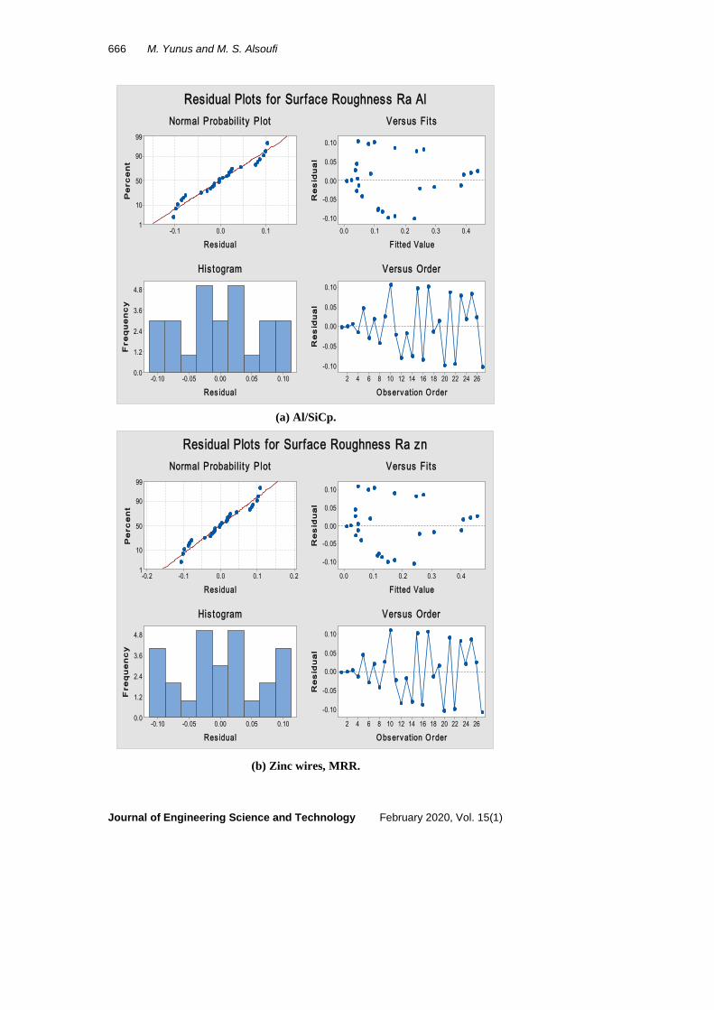
Figures 4(a) to (d) depict the fitted values and standard probability plot of residuals for the two responses of Al/SiCp and Zn materials and Fig. 3 shows the Pareto charts of responses. The residuals analysis indicates the competence of the model by the data used in that model for responses and the relationship of experimental versus predicted responses. No error is found in standard probability plots as well as residuals of outputs are minimal as they distributed across and close to the diagonal line.

Hence, they provide a fitting explanation of responses through the computation portion of the model using only the inherent arbitrariness left over within the error portion fitting the model to the experimental data. The Pareto charts show the impact of each and 2-way interaction levels of input variables for every output characteristic. The percentage of error is found less than 2% for the output characteristics using 2nd order regression models obtained by RSM optimization (refer Eqs. (1) to (4)) would help in forecasting the outputs without experimentation. Pareto charts also shown A is most significant individually, but factors at different interaction levels shown no influence, and factor F holds the least significant on all responses.

(a) Al/SiCp.

Term

EEFFDDCCBBAE

DFC

AAE

AFCECFBE

BDEBF

A

43210

A Pump PressureB Concentration of abrasives (perC Abrasive Mesh NumberD Number of CyclesE Workpiece Material

Factor Name

Standardized Effect

2.365

Pareto Chart of the Standardized Effects(Response is MRR for AlSiCp; α = 0.05)



(b) Zinc wires.

(c) AlSiCp.

(d) Zinc wires.

Fig. 3. Pareto charts for Ra.

Term

CCF

AEAFFFAADDBBEE

EDC

CECFBE

BDEBF

A

3.53.02.52.01.51.00.50.0

A Pump PressureB Concentration of abrasives (perC Abrasive Mesh NumberD Number of CyclesE Workpiece MaterialF Percentage of Oil in Media

Factor Name

Standardized Effect

2.365

Pareto Chart of the Standardized Effects(Response is MRR for Zn; α = 0.05)

Term

DDEEBBFFCC

DAAAEAF

ECF

CECFBE

BDEBF

A

43210

A Pump PressureB Concentration of abrasives (perC Abrasive Mesh NumberD Number of CyclesE Workpiece Material

Factor Name

Standardized Effect

2.365

Pareto Chart of the Standardized Effects(Response is Ra for AlSiCp; α = 0.05)

Term

EECCDDBBFFD

AEAAAF

ECF

CECFBE

BDEBF

A

43210

A Pump PressureB Concentration of abrasives (perC Abrasive Mesh NumberD Number of CyclesE Workpiece MaterialF Percentage of Oil in Media

Factor Name

Standardized Effect

2.365

Pareto Chart of the Standardized Effects(Response is Ra for zn; α = 0.05)



(a) Al/SiCp.

(b) Zinc wires, MRR.

0.10.0-0.1

99

90

50

10

1

Res idual

Pe

rce

nt

0.40.30.20.10.0

0.10

0.05

0.00

-0.05

-0.10

F itted Value

Re

sid

ua

l

0.100.050.00-0.05-0.10

4.8

3.6

2.4

1.2

0.0

Res idual

Fre

qu

en

cy

2624222018161412108642

0.10

0.05

0.00

-0.05

-0.10

Observation Order

Re

sid

ua

l

Normal Probabil i ty Plot Versus Fits

His togram Versus Order

Residual Plots for Surface Roughness Ra Al

0.20.10.0-0.1-0.2

99

90

50

10

1

Res idual

Pe

rce

nt

0.40.30.20.10.0

0.10

0.05

0.00

-0.05

-0.10

F itted Value

Re

sid

ua

l

0.100.050.00-0.05-0.10

4.8

3.6

2.4

1.2

0.0

Res idual

Fre

qu

en

cy

2624222018161412108642

0.10

0.05

0.00

-0.05

-0.10

Observation Order

Re

sid

ua

l



Residual Plots for Surface Roughness Ra zn



(c) Al/SiCp.

(d) Zinc wires.

Fig. 4. Statistical imperfection and a deterministic portion in form of fitted values and normal probability scheme of residuals for Ra.

0.10.0-0.1

99

90

50

10

1

Res idual

Pe

rce

nt

0.30.20.10.0

0.10

0.05

0.00

-0.05

-0.10

F itted Value

Re

sid

ua

l

0.080.040.00-0.04-0.08

8

6

4

2

0

Res idual

Fre

qu

en

cy

2624222018161412108642

0.10

0.05

0.00

-0.05

-0.10

Observation Order

Re

sid

ua

l



Residual Plots for Material Removal Rate for Al

0.10.0-0.1

99

90

50

10

1

Res idual

Pe

rce

nt

0.40.30.20.10.0

0.10

0.05

0.00

-0.05

-0.10

F itted Value

Re

sid

ua

l

0.100.050.00-0.05-0.10

8

6

4

2

0

Res idual

Fre

qu

en

cy

2624222018161412108642

0.10

0.05

0.00

-0.05

-0.10

Observation Order

Re

sid

ua

l



Residual Plots for Material Removal Rate for Zn



3.2. Results of RSM using BBD for responses of AFM parts As the result of using BBD method, the input parameters and the output responses that are considered for the optimization resulted in twenty-seven runs to achieve a second-order polynomial. The effects of variables on the process parameters are studied. Using Box-Behnken (BBD) design for optimizing the parameter settings, the results are compared and interpreted as follows.

BBD of RSM determined various factor levels and the effect of their interactions on performance characteristics of AFM part. Response surface plots use productive tools to examine the interaction and individual effects of input variables.

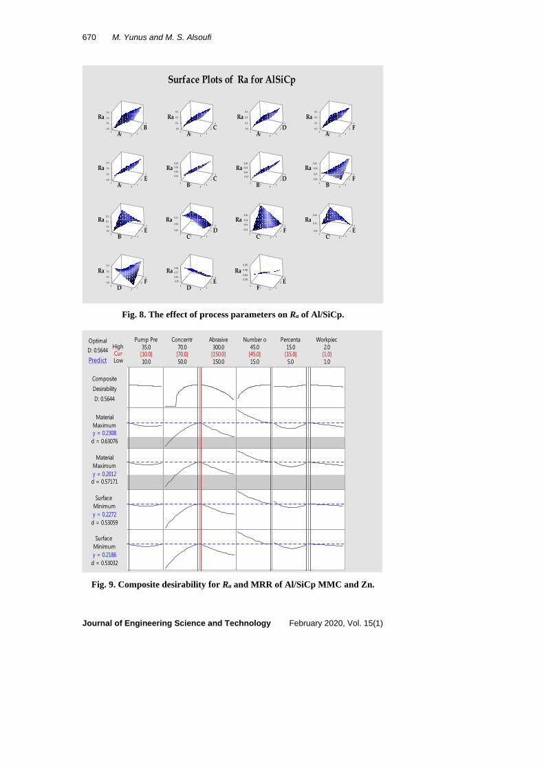
The Minitab statistical programmable software used to find optimal values when the surfaces formed by the variation of each output under various input variables. Consequently, the most significant value of responses at various optimum levels is displayed in their corresponding Figs. 5 to 8. Holding optimal input values, 3-D surface plots shows the variation of response in reaching the target either by upper and lower specified limits.

RSM analysis provides each output characteristics and its variation with varying inputs. In this RSM optimization study of the AFM responses, the objective is to jointly maximize MRR and minimizing Ra for use of a composite desirability function such that, the specific formulation for each of the inputs and outputs are shown in Fig. 9.

Fig. 5. The effect of process parameters on MRR of Al/SiCp.

12

0.0

0.13

2

13

0.2RRM

BA

0 01

2

0.0

0.13

2

13

0.2

RRM

CA 1

2

0.05

01.051.0

3

2

13

510

0.0 2

RRM

DA 1

2

0.0

1.03

2

13

0.2

RRM

FA

12

0.0

.103

2

13

0.2

RRM

EA 1

2

01.0

21.0

0

3

2

13

1.0 4

16.0

RRM

CB 1

2

0.10

. 210

.10 4

13

3

2

33

10 4

61.0

RRM

DB 1

2

. 010

0.15

13

3

2

33

0.20

RRM

FB

0 01

2

0.0

1.0

0 2.

13

2

3

0 2

0.3

RRM

EB

15.0 1

0.120

. 50 21

12 13

3

2

33

0.130

RRM

DC 1

2

0.10

.120

41.0

13

3

2

33

410

0.16

RRM

FC 1

2

80.0

0. 21

13

2

3

0 61.

RRM

EC

12

0.05.100

50.1

2

13

3

2

33

02.0

RRM

FD 1

2

. 01200.125

030 1.

2

13

3

2

33

31.0 5RRM

ED

01

2

11.0

.120

31.0

2

13

3

2

33

41.0

RRM

EF

pCiSlA rof RRM fo stolP ecafruS



Fig. 6. The effect of process parameters on MRR of Zn wire.

Fig. 7. The effect of process parameters on Ra of Zn wire.

12

33.5-0.33-5.23-

13

3

2

33

5230.23-

RRM

BA

3271- . 52

-17.0057.61-

1

-16.50

2 13

RRM

CA 1

2

-61.09.06-

-60.83

2

13

60 8-60.7

RRM

DA 1

2

-5655-

13

3

2

33

55--54

RRM

FA

12

405006

2

13

3

2

33

0670

RRM

EA

5

6

12

2

13

3

2

33

6

7

RRM

CB 1

2

0.93-.3- 580-38.

2

13

3

2

33

0385.73-

RRM

DB

63-43-23-

12

2

13

3

2

33

2303-

RRM

FB

512052

12 13

2

3

5203

RRM

EB

2 8.- 2-22.6-22.4

12 13

3

2

33

22 4-22.2

RRM

DC 1

2

- 12-18

51

13

3

2

33

51--12

RRM

FC

5230

12 13

2

3

53RRM

EC

12

-64-62-60

2

13

3

2

33

6085-

RRM

FD

034005

12

2

13

3

2

33

0506

RRM

ED 1

2

405006

2

13

3

2

33

0607

RRM

EF

nZ rof RRM fo stolP ecafruS

0 01

2

0.0

1.0

2.0

3

2

13

20

30.

aRB

A.00

12

.00

0 1.

2.0

3

2

13

20

.0 3

aRC

A.00

12

.00

0 1.

2.0

3

2

13

20

.0 3

aRD

A.00

12

.00

1.0

2.0

3

2

13

20

30.

aRF

A

0.01

2

0.0

0.1

2.0

3

2

13

20

3.0

aRE

A 12

41.061.0

81.0

3

2

13

81002.0

aR

CB 1

2

.0 14

1.0 6

.180

3

2

13

18020.0aR

DB

001

2

01.0

.0 15

0.20

2

13

3

2

33

0 20

0.25

aR

FB

001

2

.00

.10

2.0

2

13

2

3

0.3aR

EB

0 61.

0.17

12

2

13

3

2

33

81.0

aR

DC

01

2

410.

610.

0 81.

2

13

3

2

33

02.0aR

FC

001

2

01.0

0.15

2

13

2

3

0.20

aR

EC

0.01

2

0.0

0 1.

0.2

2

13

3

2

33

0.3

aRF

D 12

60 1.

1.0 7

0.18

2

13

3

2

33

0 181.0 9

aR

ED 1

2

0.1 05

561.0

0.180

2

13

3

2

33

0 180

591.0

aR

EF

nz rof aR fo stolP ecafruS



Fig. 8. The effect of process parameters on Ra of Al/SiCp.

Fig. 9. Composite desirability for Ra and MRR of Al/SiCp MMC and Zn.

0.01

2

0.0

1.0

2.0

3

2

13

20

30.

aR

BA

0.01

2

0.0

1.0

2.0

3

2

13

20

3.0

aR

CA

0.01

2

0.0

1.0

2.0

3

2

13

20

0 3.

aR

DA

0.01

2

0.0

1.0

2.0

3

2

13

20

30.

aR

FA

0.01

2

0.0

1.0

.0 2

3

2

13

0 2

3.0

aR

EA 1

2

40.1

0.16

.0 18

3

2

13

.0 1800.2

aR

CB 1

2

1.0 4

0.16

.0 18

3

2

13

0 18

00.2

aR

DB 1

2

01.0

.0 15

0.20

13

3

2

33

0 20

0. 52

aR

FB

12

.00

.10

2.0

13

2

3

0.3

aR

EB

0 51.

1.0 6

12 13

3

2

33

0.17aR

DC 1

2

14.0

0.16

18.0

13

3

2

33

180

.0 20

aR

FC 1

2

1.0 0

150.

13

2

3

0.20

aR

EC

0.01

2

0.0

0 1.

0.2

13

3

2

33

0 2

0.3

aR

FD 1

2

0.15

16.0

71.0

13

3

2

33

18.0aR

ED 1

2

051.0

16. 50

80. 0

13

3

2

33

80.1 0

0.195

aR

EF

pCiSlA rof aR fo stolP ecafruS

CurHigh

LowD: 0.5644Optimal

Predict

d = 0.63076

Maximumy = 0.2308

Material

d = 0.57171

Maximumy = 0.2012

Material

d = 0.53059

Minimumy = 0.2272

Surface

d = 0.53032

Minimumy = 0.2186

Surface

D: 0.5644DesirabilityComposite

1.0

2.0

5.0

15.0

15.0

45.0

150.0

300.0

50.0

70.0

10.0

35.0Concentr Abrasive Number o Percenta WorkpiecPump Pre

[10.0] [70.0] [150.0] [45.0] [15.0] [1.0]



Figures 9 shows the results of combined responses when composite desirability (CD) function is applied. The optimal CD of all input variables and outputs are listed: (a) Optimal results for parameters and responses (Solution: 1; A: 10; B: 70; C: 150; D: 45; E: 15; F: Zn; MRR for Zn Fit: 0.2308; MRR for Al/SiCp Fit: 0.2012; Ra for Zn Fit: 0.2272; Ra for AlSiCp Fit: 0.2186; Composite desirability: 0.564395) and (b) Optimal set of input parameters (Variable A, Setting 10; Variable B: Setting 50; Variable C, Setting 150; Variable D, Setting: 45; Variable E, Setting: 15; Variable F, Setting: 5).

This optimal set value of the system achieved by geometric average maximization of MRR and minimization of Ra was evaluated from the character desirability (d) of each output, as shown in Table 4. The AFM finishing process is considered as completely optimized because both CD and d values are seen very close to the optimal state of 1. Thus, outputs of the process for the predicted optimal condition are in good conformity with the requisite specifications. The Ra and MRR for Al/SiCp and Zn at 95% confidence and prediction intervals are listed in Table 5.

Table 5. Confirmation experiment results. Response Fit SE Fit 95% CI 95% PI

MRR of Zn 0.2224 0.0607 (0.0739; 0.3709) (0.0022; 0.4426) MRR of Al/SiCp 0.1763 0.0606 (0.0279; 0.3247) (-0.0437; 0.3963) Ra of Zn 0.2320 0.0724 (0.0549; 0.4091) (-0.0306; 0.4945) Ra of Al/SiCp 0.2219 0.0696 (0.0516; 0.3921) (-0.0305; 0.4742)

4. Conclusion The research paper presented a study based on the statistical analysis of our work using modern techniques such as ANOVA and RSM using BBD for data analysis and validation of the obtained results. A plain yet all-around AFM machine setup has successfully been developed with integral features of varying the input parameters to aid the parametric study and evaluation of the process. The effect of parameter A (pump pressure) compared to the effect of parameters B, C, D, E and F (abrasive % concentration, abrasive mesh size, number of cycles, oil concentration and workpiece material) on the responses is found to be significant input variable. RSM based experimental study concludes as follows:

• Pump/fluid pressure, the factor “A” alone was found important which affect the MRR and Ra simultaneously during multi optimization of responses.

• The variation of MRR and Ra found from 2.2 to 8 µg/s and 0.5 to 2 µm respectively. • The percentage of error found between the predicted and experimental

values of MRR holds 6.02% and 6.5% for Ra has been validated by confirmation results.

• The optimal values of the combination of factors pump pressure (A) 33.7307 MPa, concentration of abrasive; (B) 50%, abrasive mesh size; (C) 150 mesh number, number of cycles; (D) 45, workpiece material; (E) zinc and oil concentration (F) 15.

Hence, RSM provides a complete analysis of AFM machining process in both metallic and non- homogeneous materials.



References 1. Alsoufi, M.S. (2017). State-of-the-art in abrasive water jet cutting technology

and the promise for micro- and nano-machining. International Journal of Mechanical Engineering and Applications, 5(1), 1-14.

2. Alsoufi, M.S.; Suker, D.K.; Alhazmi, M.W.; and Azam, S. (2017). Abrasive waterjet machining of thick carrara marble: cutting performance vs. profile, lagging and waterjet angle assessments. Materials Sciences and Applications, 8(5), 361-375.

3. Alsoufi, M.S.; Suker, D.K.; Alhazmi, M.W.; and Azam, S. (2017). Influence of abrasive waterjet machining parameters on the surface texture quality of carrara marble. Journal of Surface Engineered Materials and Advanced Technology, 7(2), 25-37.

4. Sushil, M.; Vinod, K.; and Harmesh, K. (2018). Multi-objective optimization of process parameters involved in micro-finishing of Al/SiC MMCs by abrasive flow machining process. Proceedings of the Institution of Mechanical Engineers, Part L: Journal of Materials Design and Applications, 232(4), 319-332.

5. Gorana, V.K.; Jain, V.K.; and Lal, G.K. (2004). Experimental investigation into cutting forces and active grain density during abrasive flow machining. International Journal of Machine Tools and Manufacture, 44(2-3), 201-211.

6. Howard, M.; and Cheng, K. (2014). An integrated systematic investigation of the process variables on surface generation in abrasive flow machining of titanium alloy 6Al4V. Proceedings of the Institution of Mechanical Engineers, Part B: Journal of Engineering Manufacture, 228(11), 1419-1431.

7. Wang, A.C.; and Weng, S.H. (2007). Developing the polymer abrasive gels in AFM processs. Journal of Materials Processing Technology, 192-193, 486-490.

8. Singh, S.; and Shan, H.S. (2002). Development of magneto abrasive flow machining process. International Journal of Machine Tools and Manufacture, 42(8), 953-959.

9. Jain, R.K.; Jain, V.K.; and Dixit, P.M. (1999). Modeling of material removal and surface roughness in abrasive flow machining process. International Journal of Machine Tools and Manufacture, 39(12), 1903-1923.

10. Ko, S.L.; Baron, Y.M.; and Park, J.I. (2007). Micro deburring for precision parts using magnetic abrasive finishing method. Journal of Materials Processing Technology, 187-188, 19-25.

11. Wani, A.M.; Yadava, V.; and Khatri, A. (2007). Simulation for the prediction of surface roughness in magnetic abrasive flow finishing (MAFF). Journal of Materials Processing Technology, 190(1-3), 282-290.

12. Sadiq, A.; and Shunmugam, M.S. (2010). A novel method to improve finish on non-magnetic surfaces in magneto-rheological abrasive honing process. Tribology International, 43(5-6), 1122-1126.

13. Sankar, M.R.; Jain, V.K.; and Ramkumar, J. (2010). Rotational abrasive flow finishing (R-AFF) process and its effects on finished surface



topography. International Journal of Machine Tools and Manufacture, 50(7), 637-650.

14. Sankar, M.R.; Jain, V.K.; Ramkumar, J.; and Joshi, Y.M. (2011). Rheological characterization of styrene-butadiene based medium and its finishing performance using rotational abrasive flow finishing process. International Journal of Machine Tools and Manufacture, 51(12), 947-957.

15. Tzeng, H.-J.; Yan, B.-H.; Hsu, R.-T.; and Lin, Y.-C. (2007). Self-modulating abrasive medium and its application to abrasive flow machining for finishing micro channel surfaces. International Journal of Advanced Manufacturing Technology, 32(11), 1163-1169.

16. Mulik, R.S.; and Pandey, P.M. (2012). Experimental investigations and modeling of finishing force and torque in ultrasonic assisted magnetic abrasive finishing. Journal of Manufacturing Science and Engineering, 134(5), 12 pages.

17. Bhardwaj, B.; Kumar, R.; and Singh, P.K. (2014). Surface roughness (Ra) prediction model for turning of AISI 1019 steel using response surface methodology and Box-Cox transformation. Proceedings of the Institution of Mechanical Engineers, Part B: Journal of Engineering Manufacture, 228(2), 223-232.

18. Jain, R.K.; and Jain, V.K. (2000). Optimum selection of machining conditions in abrasive flow machining using neural network. Journal of Materials Processing Technology, 108(1), 62-67.

19. Karagiannis, S.; Stafropoulos, P.; Ziogas, C.; and Kechagias, J. (2014). Prediction of surface roughness magnitude in computer numerical controlled end milling processes using neural networks, by considering a set of influence parameters: An aluminium alloy 5083 case study. Proceedings of the Institution of Mechanical Engineers, Part B: Journal of Engineering Manufacture, 228(2), 233-244.

20. Fletcher, A.J.; Hull, J.B.; Mackie, J.; and Trengove, S.A. (1990). Computer modelling of the abrasive flow machining process. Surface Engineering, 592-601.

21. Cherian, J.; and Issac, J.M. (2013). Effect of process variables in abrasive flow machining. International Journal of Emerging Technology and Advanced Engineering, 3(2), 554-557.

22. Jain, R.K.; and Jain, V.K. (1999). Abrasive fine finishing processes - a review. International Journal of Manufacturing Science and Production, 2(1), 55-68.

23. Yunus, M.; Alsoufi, M.S.; and Irfan, M. (2016). Application of QC tools for continuous improvement in an expensive seat hardfacing process using tig welding. International Journal for Quality Research, 10(3), 641-660.

24. Hiremath, S.S.; Vidyadhar, H.M.; and Singaperumal, M. (2013). A novel approach for finishing internal complex features using developed abrasive flow finishing machine. International Journal of Recent Advances in Mechanical Engineering (IJMECH), 2(4), 37-44.



25. Loveless, T.R.; Williams, R.E.; and Rajurkar, K.P. (1994). A study of the effects of abrasive-flow finishing on various machined surfaces. Journal of Materials Processing Technology, 47(1-2), 133-151.

26. Panda, A.; Sahoo, A.K.; and Rout, A.K. (2017). Machining performance assessment of hardened AISI 52100 steel using multilayer coated carbide insert. Journal of Engineering Science and Technology (JESTEC), 12(6), 1488-1505.

27. Yunus, M.; and Alsoufi, M.S. (2019). Mathematical modeling of multiple quality characteristics of a laser microdrilling process used in Al7075/SiCp metal matrix composite using genetic programming. Modelling and Simulation in Engineering, Article ID 1024365, 15 pages.

28. Yunus, M.; and Alsoufi, M.S. (2018). Experimental investigations into the mechanical, tribological, and corrosion properties of hybrid polymer matrix composites comprising ceramic reinforcement for biomedical applications. International Journal of Biomaterials, Article ID 9283291, 8 pages.

application of response surface methodology for …jestec.taylors.edu.my/vol 15 issue 1 february...

Documents