application of pole decomposition to an equation governing...
TRANSCRIPT

Application of pole decomposition to an equation
governing the dynamics of wrinkled flame fronts
O. Thual, U. Frisch, M. Henon
To cite this version:
O. Thual, U. Frisch, M. Henon. Application of pole decomposition to an equation govern-ing the dynamics of wrinkled flame fronts. Journal de Physique, 1985, 46 (9), pp.1485-1494.<10.1051/jphys:019850046090148500>. <jpa-00210093>
HAL Id: jpa-00210093
https://hal.archives-ouvertes.fr/jpa-00210093
Submitted on 1 Jan 1985
HAL is a multi-disciplinary open accessarchive for the deposit and dissemination of sci-entific research documents, whether they are pub-lished or not. The documents may come fromteaching and research institutions in France orabroad, or from public or private research centers.
L’archive ouverte pluridisciplinaire HAL, estdestinee au depot et a la diffusion de documentsscientifiques de niveau recherche, publies ou non,emanant des etablissements d’enseignement et derecherche francais ou etrangers, des laboratoirespublics ou prives.
1485
Application of pole decomposition to an equationgoverning the dynamics of wrinkled flame fronts
O. Thual
CNRM, 42 avenue Coriolis, 31057 Toulouse Cedex, France
U. Frisch and M. Hénon
CNRS, Observatoire de Nice, B.P.139, 06003 Nice Cedex, France
(Reçu le 27 fevrier 1985, accepté le 13 mai 1985)
Résumé. 2014 L’équation intégrale de Sivashinsky gouvernant certaines instabilités hydrodynamiques de fronts deflamme unidimensionnels est un cas particulier des modèles de plasma non linéaires de Lee et Chen; en tant quetelle elle possède une décomposition en pôles. Ceci explique les structures très organisées observées dans les simu-lations numériques. L’équation de Sivashinsky a des solutions stationnaires stables avec les pôles alignés parallèle-ment à l’axe imaginaire. Avec des conditions aux limites périodiques, quand le nombre de modes linéairementinstables est élevé, les pôles se condensent en une distribution In coth. Ceci est illustré par calcul numérique despositions d’équilibre des pôles. La condensation des pôles explique les plis de certains fronts de flamme. Le spectred’ énergie du déplacement du front suit une loi en ln2 k.
Abstract. 2014 The Sivashinsky integral equation governing certain hydrodynamical instabilities of one-dimensionalflame fronts is a special case of Lee and Chen’s (Phys. Scr. 2 (1982) 41) non linear plasma models; as such it has apole decomposition. This explains the highly organized structures observed in numerical simulations. The Sivas-hinsky equation has stable steady solutions with the poles aligned parallel to the imaginary axis. With periodicboundary conditions, when the number of linearly unstable modes is large, the poles condense into a In cothdistribution. This is illustrated by numerical calculations of equilibrium positions of poles. The pole condensationexplains cusp-like wrinkles in certain flame fronts. The energy spectrum for the front displacement follows aIn2 k law.
J. Physique 46 (1985) 1485-1494 SEPTEMBRE 1985,
Classification
Physics Abstracts05.45 - 47.20 - 47.70F
1. Introduction.
Sivashinsky [1] has shown that in a suitable asymptoticregime the dynamics of wrinkled flame fronts is
governed by a non linear partial (pseudo)differentialequation. In the one-dimensional case it reads
tl is a linear singular operator defined convenientlyin terms of the spatial Fourier transform :
We here use notation different from Sivashinsky’s
in order to bring out similarities with Burgers’ equa-tion
What is here denoted u is actually not a velocity but0.0 where 0 is the flame front displacement; so it isthe slope of the flame front. Also we find it more con-venient to vary the « viscosity » v rather than the sizeof the domain.
Various studies of the Sivashinsky equation havebeen reported [1-4]. The results indicate that thesolutions are highly organized in the form of oneor several wrinkles (see Figs. 2 and 3 of Ref. [3] and alsoFigs. 2 and 3 of the present paper).At the root of this simple behaviour of the Siva-
shinsky equation is the fact that it possesses a poledecomposition : equation (1.1) admits solutions of the
Article published online by EDP Sciences and available at http://dx.doi.org/10.1051/jphys:019850046090148500

1486
form
The z.’s are poles in the complex plane (coming in c.c.pairs) moving according to the laws of motion ofpoles (a = 1, 2,..., 2 N)
where 3 denotes the imaginary part. When 2 re spatialperiodicity is assumed it is enough to restrict atten-tion to poles with real parts between 0 and 2 re. Insteadof equations (1. 5) and (1.6) one then uses
and
The existence of this pole decomposition followsfrom a more general result of Lee and Chen [5] for aclass of non linear dynamical models arising in
plasma turbulence. In our notation the governingequations for the Lee and Chen models are
which is a linear combination of the Sivashinskyequation and the Benjamin-Ono [6-7] equation. Forthe convenience of the reader a derivation of the poledecomposition for the Sivashinsky equation is givenin the appendix A.We shall not here review work on pole decomposi-
tions. A list of references up to 1981 may be foundin section 4 of reference [8]. We also mention a recentapplication of pole decomposition to the formationof cusp singularities in interface dynamics [9].
This paper is organized as follows : section 2 is asystematic study of the two pole problem giving somequalitative insight into N-pole dynamics; in particularthere is a tendency for the poles to align themselvesparallel to the imaginary axis. Subsequently the paperis devoted essentially to the detailed study of such« vertical alignments ». Section 3 is about the discretedynamics of N pairs of poles : for N large the polescondense into a continuous distribution which isdetermined analytically (Sect. 4). This is the analogfor the Sivashinsky equation of the pole condensationsfor Burgers’ equation [10]. From the distribution ofpoles we deduce the shape of flame wrinkles and thehigh wavenumber behaviour of the energy spectrum.In section 5 we mention some implications and openproblems.
2. The two-pole problem and qualitative dynamics.We begin by studying the simplest dynamical situa-tion with two poles at complex conjugate locationsz(t) = a(t) + ib(t) and z* = a - ib with b > 0. From
equation (1.6), we have
It follows that a is a constant and that
Note that the - 2 v/(z - z*) term in equation (2.1),already present in Burgers’ dynamics, tends to pushthe poles away from the real axis while the - i termproduces a uniform drift towards the real axis. Theircompetition leads for t -+ oo to a stable equilibriumconfiguration with
beq = v . (2. 3)
The corresponding steady solution of the Sivashinskyequation is
In the periodic case equations (2.3) and (2.4) becomerespectively
and
A graph of u(x) for v = 5 x 10⁻² is shown in figure 1.The aspect is quite similar to the localized structuresappearing in figure 3 of reference [4], concerning anequation differing very slightly from the Sivashinskyequation.Next we consider two poles z1 and z2 in the
upper half plane 3(z) > 0 which we assume to be
sufficiently close to each other so that we can ignoretheir interactions with other poles. We then have
When t varies from 0 to + oo, then j(C2) = 2 abremains constant so that the point (a, b) moves on a

1487
Fig. 1. - Structure of the slope of the flame front u(x)for the steady space-periodic solution with two complexconjugate poles.
hyperbola. For large times a - 0 and b --i. + oo :
poles tend to align on a parallel to the imaginary axis.The above analysis indicates that, roughly, poles
tend to attract each other horizontally (parallel to thereal axis) and to repel each other vertically. In addi-tion, they are subject to a drift towards the real axis.Extrapolation of these qualitative features to a
situation with many poles suggests that the poles tendto form vertical alignments, eventually coalescinginto a single one. This is indeed happening in Burgers’dynamics and may be viewed as the mechanism forthe formation and coalescence of shocks. Accordingto Lee and Chen [5] this merging process is a universalproperty of their non dispersive models.
In the periodic case the poles are constrained to beon 2 x periodic arrays or, equivalently, to be allcontained in a domain of extension 2 x in the realdirection and to have cot rather than z-1 interactions.The short distance behaviour is thus unaffected, butthe global dynamics are quite different. At the momentthere is no result concerning the eventual fate of asystem of poles (periodic or non periodic). In theperiodic case numerical integrations of the Sivas-hinsky equation [3-4] indicate that for small v thesolutions often tend to a steady state with one orseveral wrinkles in the flame front displacement (infact vertical pole condensations as we shall see).These features are reproduced in simulations of ourown using a pseudo-spectral method with 512 Fou-rier modes. Figure 2 shows a solution with one wrinklefor v = 0.1. Figure 3 shows a solution with two
wrinkles, also for v = 0.1, but restricted to the classof functions u(x) which are odd (otherwise this solu-tion would be unstable). The labels a and b corres-
Fig. 2. - Structure of the flame front (a) and its slope (b)for a steady one-wrinkle space-periodic solution obtainedby pseudo-spectral simulation of the Sivashinsky equationwith 512 Fourier modes and « viscosity ? coefficient v = 0.1.
pond respectively to the front displacement O(x)and the front slope u(x).
Henceforth we shall consider a single vertical
alignment, possibly containing a large number ofpoles, with or without periodicity.
3. Vertical alignments of poles : discrete dynamics.We consider N pairs of complex conjugate polesconstrained to be on a parallel to the imaginary axis,located at

1488
Fig. 3. - Same as figure 2, except that the solution
u(x) is restricted to odd functions, allowing stable coexis-tence of two wrinkles.
Without loss of generality, we assume that xo = 0;we also assume that the y J’s have been ordered :
This order will never change since the repulsion bet-ween two poles becomes infinite when they approacheach other. For the same reason, we always havestrict inequalities in (3.2).The motion of poles is given by a set of N simul-
taneous real differential equations :
with, in the non-periodic case
and in the periodic case
For N = 1, (3.4) reduces to (2.2). A steady state willbe a solution of the N simultaneous ordinary equations
f = 0 (i = 1,..., N). (3 . 6)
We note first some properties of these equations.(i) In the non-periodic case, v can be eliminated
by the change of variables
v is therefore an irrelevant parameter. On the contrary,in the periodic case a scale is prescribed so that thevalue of v is relevant.
(ii) In the non-periodic case, multiplying (3.4)by yj and summing over j, we obtain the virial-likerelation
The right-hand side must vanish at equilibrium;this provides a test of computational accuracy.
(iii) In the periodic case, we derive from (3.5)for the highest pole j = N, using the fact that
If the right-hand side is positive or zero, fN is alwayspositive, and no steady state can exist; the highestpole moves towards y = + oo in the imaginary direc-tion with an (asymptotically) constant speed. There-fore a necessary condition for the existence of a steadystate in the periodic case is
(iv) The following properties hold in the non-perio-dic case, and also in the periodic case when (3.10) issatisfied :
1. There exists one and only one steady state.2. Any solution of (3.3) tends towards the steady
state for t - + oo. The proof of these properties isbased on the existence of a Lyapunov function (seeAppendix B).
(v) The equations (3.6) are easily solved forN = 1, 2, 3 in the non-periodic case. We take v = 1for simplicity. For N = 1, the steady state solution is

1489
For N = 3, the yj are the three roots of the equation
These valus can also be used as a check on the pro-gram for the numerical solution of (3.6).We turn now to numerical determination of the
equilibrium positions. The equations (3.6) were
solved numerically by a relaxation method : the
position yi of each pole in turn is adjusted to a newvalue
Ayj is computed by a one-step Newton formula :
with the constraint that it should not exceed one-half of the distance to the next pole. A convenientinitial state is : yj = 2 vj. The computation is haltedwhen the relative changes I Ayi llyj becomes less thansome prescribed small number for all poles. Thismethod was found to always converge to the equili-brium, although the convergence slows down for
large N.The value
was used in all numerical computations, in order tofacilitate comparisons. As a consequence of (3.10), asmall value of v is necessary in order to allow a largenumber of poles in the periodic case. With the value(3. 17), the maximum of N in the periodic case is
Figures 4a and 4b show (full curves) the cumulativedistribution, i.e., the number of poles between 0 andy as a function of y, for the non-periodic case and forN = 10 and N = 100 respectively. The dotted anddashed curves are analytic approximations whichwill be described in section 4. Table I gives in columns 2
Fig. 4. - Cumulative distribution of poles along the ima-ginary axis in the non-periodic case. Full curve (staircase) :discrete distribution for (a) N = 10, (b) N = 100. Dottedand dashed curves : asymptotic distribution (4.5) withnormalization given respectively by (4. 4) and (4. ).
and 3 the positions of the lowest and highest poles,yi and yN, for various N. Column 4 is an analyticestimate which will also be described in section 4.
Table I
1490
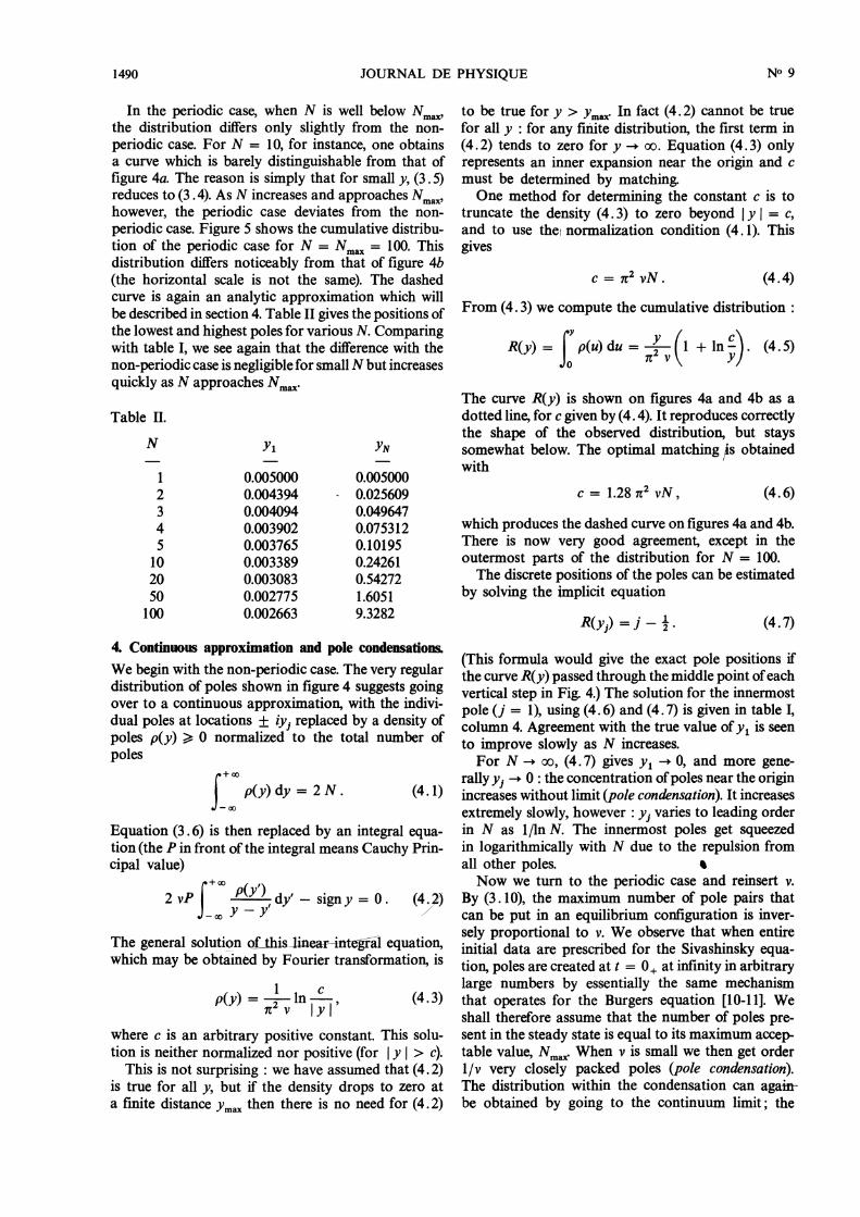
In the periodic case, when N is well below Nalthe distribution differs only slightly from the non-periodic case. For N = 10, for instance, one obtainsa curve which is barely distinguishable from that offigure 4a. The reason is simply that for small y, (3.5)reduces to (3.4). As N increases and approaches Nmax,however, the periodic case deviates from the non-periodic case. Figure 5 shows the cumulative distribu-tion of the periodic case for N = Nmax = 100. Thisdistribution differs noticeably from that of figure 4b(the horizontal scale is not the same). The dashedcurve is again an analytic approximation which willbe described in section 4. Table II gives the positions ofthe lowest and highest poles for various N. Comparingwith table I, we see again that the difference with thenon-periodic case is negligible for small N but increasesquickly as N approaches Nmax.
Table II.
N Yi YN
1 0.005000 0.0050002 0.004394 0.0256093 0.004094 0.0496474 0.003902 0.0753125 0.003765 0.1019510 0.003389 0.2426120 0.003083 0.5427250 0.002775 1.6051100 0.002663 9.3282
4. Continuous approximation and pole condensations.We begin with the non-periodic case. The very regulardistribution of poles shown in figure 4 suggests goingover to a continuous approximation, with the indivi-dual poles at locations + iyj replaced by a density ofpoles p(y) >, 0 normalized to the total number ofpoles
Equation (3.6) is then replaced by an integral equa-tion (the P in front of the integral means Cauchy Prin-cipal value)
The general solution of ° ° ° gral equation,which may be obtained by Fourier transformation, is
where c is an arbitrary positive constant. This solu-tion is neither normalized nor positive (for y > c).
This is not surprising : we have assumed that (4.2)is true for all y, but if the density drops to zero ata finite distance ymax then there is no need for (4.2)
to be true for y > Ymax. In fact (4.2) cannot be truefor all y : for any finite distribution, the first term in(4.2) tends to zero for y - oo. Equation (4. 3) onlyrepresents an inner expansion near the origin and cmust be determined by matching.One method for determining the constant c is to
truncate the density (4. 3) to zero beyond y I = c,and to use the normalization condition (4.1). Thisgives
From (4. 3) we compute the cumulative distribution :
The curve R(y) is shown on figures 4a and 4b as adotted line, for c given by (4. 4). It reproduces correctlythe shape of the observed distribution, but stayssomewhat below. The optimal matching is obtainedwith
which produces the dashed curve on figures 4a and 4b.There is now very good agreement, except in theoutermost parts of the distribution for N = 100.The discrete positions of the poles can be estimated
by solving the implicit equation
(This formula would give the exact pole positions ifthe curve R(y) passed through the middle point of eachvertical step in Fig. 4.) The solution for the innermostpole ( j = 1), using (4. 6) and (4. 7) is given in table I,column 4. Agreement with the true value of yl is seento improve slowly as N increases.For N --+ oo, (4.7) gives y1 -+ 0, and more gene-
rally yj --+ 0 : the concentration of poles near the originincreases without limit (pole condensation). It increasesextremely slowly, however : yj varies to leading orderin N as 1 /ln N. The innermost poles get squeezedin logarithmically with N due to the repulsion fromall other poles. 0
Now we turn to the periodic case and reinsert v.
By (3. 10), the maximum number of pole pairs thatcan be put in an equilibrium configuration is inver-sely proportional to v. We observe that when entireinitial data are prescribed for the Sivashinsky equa-tion, poles are created at t = 0+ at infinity in arbitrarylarge numbers by essentially the same mechanismthat operates for the Burgers equation [10-11]. Weshall therefore assume that the number of poles pre-sent in the steady state is equal to its maximum accep-table value, N Max. When v is small we then get order1 / v very closely packed poles (pole condensation).The distribution within the condensation can again-be obtained by going to the continuum limit; the

1491
analog of equation (4.2) is
The general solution is
where cl is an arbitrary positive constant. This is againan inner expansion. Since we know that there is onlya finite number of poles 0(v-1), we impose that thedensity p - 0 as y - oo. This gives
Moreover p is then positive for all y and
Since we assume N to be large and equal to themaximum value N Max allowed by (3.10), we have
so that the normalization condition (4.1) is fulfilledto leading order.We define again the cumulative distribution as
For p given by (4.9), this integral does not appearto have a closed form, so we compute it numerically.The integrand being singular at y = 0, it is convenientto do first an integration by parts :
The singularity is then isolated in the first term, andthe second term is easily evaluated numerically. Thecurve R(y) is shown on figure 5 as a dashed line.The agreement with the observed distribution isexcellent over the whole y range.Note that for small y, the density is to leading order
given by
We recover the form (4.3) of the non-periodic case,with c = 4. The best-fit solution (4.6) for the non-periodic case, together with (4.12) would have given
Fig. 5. - Cumulative distribution of poles along the ima-ginary axis in the periodic case. Full curve : discrete dis-tribution for v = 0.005, N = 100, Dashed curve : asymp-totic distribution (4.14).
Thus, for given large N, the periodic and non-periodiccases have the same functional form for R(y) neary = 0 but different normalizations. We can againestimate the position of the innermost pole yl from(4.7) and (4.14) ; since y is small, the latter can bereplaced by
for v = 0.005, we obtain from this continuous approxi-mation
to be compared with the value computed from thediscrete case
If v is varied, with N simultaneously changed so thatis always has its maximum value, then yi, the distanceof the innermost pole to the real axis, is given to leadingorder in v by
Using the above asymptotic expansions we candetermine some key features of the small v steadysolutions in the periodic case. The solution of the q
Sivashinsky equation with a pole condensation on theimaginary axis is given in real physical space by
Fori x >> v/ln (1/v)we can use the continuous density

1492
and obtain
The asymptotic expansion of this integral for (not too)small x gives
The corresponding expansion for the flame frontdisplacement §(x) is
Sivashinsky (1983) refers to a similar logarithmicsingularity at the cusps of the flame folds, obtained byMcConnaughey (1982). Actually there is no real
singularity : from equation (4.20) the closest complexsingularity is within a distance y, = 0(v/ln v-1) ;thus the cusp is slightly rounded over a distance yl.We now calculate the spectrum E(k) of the solution,
defined as the squared modulus of the Fourier trans-form of the steady flame front displacement. Sinceu(x) = O.,,O(x) we have
where
A simple residue calculation based on the pole de-composition gives, for k > 0
For large k we must distinguish two ranges :(i) Dissipation range. When I k y1 >> 1 only the
nearest pole singularity matters and we get
with y1 given by equation (4.20).(ii) Inertial range. When 1 k y1-1 we may
replace the sum in equation (4.27) by an integral overthe continuous distribution of poles; this gives toleading order (for v -+ 0 first and then k -+ oo)
Note that the energy spectrum for u(x) follows ak- 2 In2 I k I law; i.e. it is somewhat shallower thanthe k-2 spectrum obtained for Burgers’ model. Thenumerical simulation of Pumir [4] (his Fig. 5b) givesfor u(x) an energy spectrum that approximately
follows a k-a law with a N 1.23 which is also shallowerthan k-2. Given that Pumir’s equation is not exactlythe Sivashinsky equation and given also the limitedrange of wavenumbers involved there is probably nogenuine discrepancy.
5. Discussion.
We have found that the pole decomposition providesa reduction of the Sivashinsky equation to a discreteDynamical System. The latter admits steady state
solutions with all the poles aligned parallel to theimaginary axis. In the spatially periodic case themaximum number N of complex conjugate pairs ofpoles in an alignment is such that v(2 N - 1) 1.We conjecture more general results for analyticperiodic initial data : (i) as t -+ oo all the singularities(poles and others) are pushed off to infinity, excepta finite number N of pairs of poles satisfying the aboveinequality; (ii) for real times poles stay uniformlybounded away from the real axis. The former resulthas been recently established for the case of initialconditions with a finite but arbitrary number of poles[13, 14]. In this context we also mention a result ofFoias, Nicolaenko, Sell and Temam [17] concerningthe family of equations
where the operator M. has the following represen-tation in Fourier space
It is assumed that 0 8 1; 8 = 1 is the Sivashinskyequation. For the case of space-periodic odd solutionsof equation (5. 2) Foias et al. [15] have shown thatwhen t -+ cc the solutions have a finite dimensionalattractor imbedded in a finite dimensional manifold
In the periodic case with small v we found that thepoles on a vertical alignment condense into a In cothdistribution the signature of which in real physicalspace is a cusp in the flame front. This suggests a realsingularity. Actually, as we have seen in section 4there are only complex poles, but the ones nearest tothe real axis are at a distance 0(v/ln v-1) so that thecusp is slightly rounded. It is noteworthy that thisdistance is smaller by a factor 1/ln v-1 to what wouldhave been inferred from a naive analysis based on theobservation that wavenumbers in excess of, v-1 arelinearly stable. This discrepancy is important whenattempting to numerically solve the Sivashinskyequation : the number of Fourier modes that arenecessary scales like v-1 ln v-1 and not like v-1.Otherwise the numerics will work well as long as thepoles stay within 0(v) of the real axis (as in the two-pole solution); after some time however the poleswill start piling up vertically and spurious singularitiesmay be observed [4].

1493
We finally mention an open problem. We haveshown that the Sivashinsky equation has stable steadysolutions, which can be made trivially time-dependentby a Galilean transformation. There may also be non-trivial time-dependent solutions. In one spectralsimulation with 25 linearly unstable modes (v = 1/25)we have observed a complicated time-dependentregime going through a succession of single andmulti-wrinkle configurations. At the moment wecannot rule out ever-lasting, possibly chaotic, time-dependent solutions [16].
Acknowledgments.We have benefitted from discussions with Y. C. Lee,A. Pumir, B. Nicolaenko, and S. Zaleski. Some ofthe numerical results reported in section 3 wereobtained independently by J. P. Rivet
Appendix A.
THE POLE DECOMPOSITION. - We wish to show that
equations (1.1)-(1.3) have pole solutions of the form
where A is the pseudo-differential operator definedby (1. 3), i.e. multiplication by k I in Fourier space.A simple residue calculation gives the followingexpression for the Fourier transform pz(k) of pz(x) :
where H(.) is the Heavyside function. Thus pz(k)has its support in the negative or positive k-axis,depending on the sign of the imaginary part of z.Since the Fourier transform of 0,, is the multiplicationby ik (see (1. 2)), the operator A acting on the functionpz is equivalent to ± iax. This proves (A. 4). We maythus interpret the operator A in the Sivashinskyequation (1.1) as producing an advection in the
complex plane, in the imaginary direction towardsthe real axis.
Finally, the proof that (A. 1) and (A. 2) satisfies theSivashinsky equation (1.1) is obtained by substitutionand straightforward algebra, using the identity
- 2 1
with
We note that u(x) is a linear combination of terms ofthe form
We claim that
Appendix B.
We give here the proofs of the assertions made insection 3. We remark first that the differential equa-tions (3.3) may be written in terms of a Lyapunovfunction U :
with, in the non-periodic case :
and in the periodic case :
A simple computation shows that the function
U( y1, ..., yN) has a negative curvature in every direc-tion. Specifically, if we consider a linear displacement :yj = a. + hj v, with aj, bj constants and v variable,then d2Uldv2 0. An immediate consequence isthat there cannot exist more than one steady state :if two existed, on the straight-line segment joiningthem we would have d Uldv = 0 at each end, which is incontradiction with the above property. Another
consequence is that if a steady state does exist, thenit is a global maximum for U.Next we show that a steady state actually exists
(provided, in the periodic case, that the inequality(3.10) holds). We consider a sub-problem in whichyp , 1, ..., YN have given values while yl, ..., yp are free,and we look for a steady state for the free variables.Specifically, we look for values of Yl’ ..., yp such that(3.6) is satisfied for j = 1, ..., p. The accessible phase

1494
space is :
The same reasoning as above shows that there cannotexist more than one equilibrium for y,, ..., yp. Weshow now by recursion that one exists. Considerfirst the case p = 1. The domain of variation of Y 1 is0 yi y2. For y, -+ 0, f1 -+ + oo ; and for y1 y2,f1 - - oo. Therefore there exists a yi for which £vanishes, i.e., a steady state for Y 1. Suppose now thatwe have proved the existence of a steady state for p -1poles and we want to prove it for p poles, with p N.We let yp vary in the interval 0 Yp yp , 1, withthe other poles yl, ..., Yp-l continually adjusted totheir equilibrium position. For yp -+ 0, f p -+ + oo ;and for yp -+ yp + 1, fp --+ - oo (it is easily. seen thatthe distance yp - yp-1 remains finite in the limit).Therefore there exists a yp for which fp = 0.The last case p = N, is treated in the same fashion
but with a slight difference. The interval of variation
is now 0 yN oo. For yN - oo, fN -+ - 1 in the
non-periodic case, and fN -+ v(2 N - 1) - 1 in the
periodic case. Therefore there exists a yN for whichYN = 0. This completes the proof of existence of asteady state.
Finally, we have from (B .1) :
the equality being obtained only at a steady state.
Thus U always increases with time, except at equi-librium. On the other hand, U is bounded from aboveby its value at the steady state, which is a globalmaximum. Therefore U is a genuine Lyapunovfunction, and every solution of (3.3) tends towardthe steady state for t -+ oo. This completes the proofof stability for pole-displacements parallel to the
imaginary axis. This result has been extended to
arbitrary displacements other than the trivial oneswhere all the poles undergo a same real translation [17].
References
[1] SIVASHINSKY, G. I., Acta Astronaut. 4 (1977) 1177.[2] SIVASHINSKY, G. I., Ann. Rev. Fluid Mech. 15 (1983)
179.
[3] MICHELSON, D. M. and SIVASHINSKY, G. I., ActaAstronaut. 4 (1977) 1207.
[4] PUMIR, A., Phys. Rev. A 31 (1985) 543.[5] LEE, Y. C. and CHEN, H. H., Phys. Scr. T 2 (1982) 41.[6] BENJAMIN, T. B., J. Fluid Mech. 25 (1966) 241.[7] ONO, H., J. Phys. Soc. Japan 39 (1975) 1082.[8] FRISCH, U. and MORF, R., Phys. Rev. A 23 (1981) 2673.[9] SHRAIMAN, B. and BENSIMON, D., Phys. Rev. A 30
(1984) 2840.[10] BESSIS, D. and FOURNIER, J. D., J. Physique Lett. 45
(1984) L-833.[11] FRISCH, U. in Proceed. Sixth Kyoto Summer Institute
on Chaos and Statistical Methods, ed. Y. Kura-moto, p. 211, Springer series in Synergetics,
Springer (1984).[12] MCCONNAUGHEY, H. V., Combust. Sci. Technol. 33
(1983) 113.[13] LEE, Y. C., CHENG, H. H., LEE, T. T. and QIAN, S. N.,
Solitons and Turbulence ; Chaos in Infinite Dimen-sional Systems ; Proc. Second Intern. Workshopon Non Linear and Turbulent Processes in Physics ;Kiev, October 1983, p. 1425, Gordon and Breach.
[14] LEE, Y. C., private communication (1985).[15] FOIAS, C., NICOLAENKO, B., SELL, G. and TEMAM, R.,
Inertial Manifold for the Kuramoto-Sivashinskyequation, preprint Indiana University, Depart.Math. (1984).
[16] MICHELSON, D. M. and SIVASHINSKY, G. I., Combust.Flame 48 (1982) 211.
[17] RIVET, J. P., private communication (1985).