Application of OMA to Operational Wind Turbine: Methods for Cleaning Up the Campbell Diagram

D. Tcherniak1, C. E. Carcangiu

2, M. Rossetti

2

1 Brüel and Kjær Sound and Vibration Measurement A/S

Skodsborgvej 307, DK-2850, Naerum, Denmark

email: dtcherniak@bksv.com

2 ALSTOM WIND S.L.U.

Roc Boronat, 78, 08005 Barcelona, Spain

Abstract Engineers designing wind turbines often use Campbell diagrams as a convenient tool for representing the

dependence of wind turbine modal parameters on the rotor (and wind) speed. Experimentally obtained

Campbell diagrams are used for tuning wind turbine numerical models, which are used heavily in the

design of wind turbine structures and their control systems. Several previous studies showed that

Operational Modal Analysis (OMA) can be successfully employed for plotting experimental Campbell

diagrams. In this study, OMA is applied to a number of experimental sets of data measured under

different wind conditions. However, because several OMA assumptions are partly violated, the resulting

diagram is contaminated by computational and noise poles, which cannot be filtered out by conventional

means provided by OMA algorithms.

The presented study compares three methods for segregating the physical poles from their computational

and noise counterparts. Since the modal frequencies and damping of a wind turbine change with the rotor

speed, these modal parameters cannot be utilized for grouping the poles, as is typically done in the case of

stabilization diagrams. The mode shape vectors are utilized instead.

The first presented method uses hierarchical clustering to group the poles according to the similarity

between the associated mode shape vectors. The second method is based on the Singular Value

Decomposition (SVD) performed on an AutoMAC matrix. This method was originally suggested by other

authors for cleaning up stabilization diagrams. Finally, the third method utilizes Self-organizing Maps

(SOM) for the same purpose.

The methods are applied to the experimental data from the ALSTOM WIND ECO 100 3MW wind

turbine; the results are compared and the advantages and disadvantages of the methods are discussed.

1 Introduction

It is known [1] that modal parameters of a general structure with rotating elements will depend on their

rotational speed. In the case of operational wind turbines, modal characteristics of rotor-related modes will

depend on the rotor speed [2]. A plot representing the dependence of the modal frequencies from the rotor

speed is called a Campbell diagram; it is widely used in engineering practice.

In the case of wind turbines, an experimentally obtained Campbell diagram is an important tool for tuning

wind turbine numerical models, which are heavily used in the design of wind turbine structural elements

and their control systems [3].

Another often discussed application of modal parameters is their utilization as indicators of structural

integrity (in other words, structural health). When considering a structure health monitoring (SHM)

system based on modal parameters, it is important to take into account their dependency from the rotor

speed, which also highlights the importance of the Campbell diagram.

The latest advances in modal analysis [4] make it possible to design a robust autonomous system able to

determine modal parameters with very little or no user interaction. However, conventional experimental

modal analysis requires controlled excitation of the object under test, which is often not feasible for big

structures. Here OMA shows its advantage: relying on ambient or operational excitation, it allows for

extraction of modal parameters from response measurements only. This makes OMA attractive for

creating a modal-based SHM system which can autonomously monitor modal parameters of big structures

like buildings, towers, bridges and raise an alarm if these parameters significantly change. One example of

using OMA for autonomous health monitoring of a bridge, taking into account temperature fluctuation and

static loads, is presented in [5].

Expanding this idea to wind turbine SHM systems, one can envisage the following scenario: use OMA to

estimate modal parameters of an operational wind turbine; take into account influencing factors such as

temperature and rotor speed (Campbell diagram) and use for example a novelty detection-based decision

making system to raise an alarm if the modal parameters deviate from their normal state.

However, as it was reported in [6], in the case of operational wind turbines, several OMA assumptions are

violated. This causes OMA to produce a lot of false poles, which can be confused with structural modes.

For example, Figure 1 shows a typical stabilization diagram for an operational wind turbine obtained using

a state-of-the-art OMA time domain stochastic subspace iteration (SSI) algorithm. An attempt to generate

an experimental Campbell diagram applying OMA to a large number of datasets measured at different

wind speeds (and hence rotor RPM) leads to a very noisy plot (Figure 2a), which is useless for practical

purposes.

This problem calls for a technique which is able to select poles corresponding to the structural modes of

the wind turbine, group these poles (that were obtained at different wind speeds) together and, by

discarding the non-physical poles, clean up the Campbell diagram. An example of a cleaned up Campbell

diagram is shown in Figure 2b.

The problem formulated above belongs to the class of those typically posed for different classification

and clustering techniques widely used in data mining. The current study presents three different clustering

techniques; the focus is on their robustness and ability to be used as a part of an autonomous SHM system

which can operate with no (or very little) user interaction. The first method uses so-called hierarchical

clustering to group the poles according to the distance, which is proportional to the values of the

AutoMAC matrix. Chronologically, it was the first method which was applied to clean up the Campbell

diagram for the ALSTOM Wind ECO 100 wind turbine; the results were published in [7]. The method

performed satisfactorily; the results obtained from this method serve as a baseline for comparison with the

other two considered methods. However the method required a lot of user interaction which initiated the

search for more autonomous methods.

Frequency

Figure 1. A typical stabilization diagram obtained by OMA Crystal Clear® SSI (Unweighted Principal Component) applied to data measured on an operational wind turbine.

The second method is based on Singular Value Decomposition (SVD) performed on an AutoMAC matrix.

This method was originally suggested for cleaning stabilization diagrams [4]. The third method utilizes a

Self-organizing Map (SOM) for the same purpose.

The study demonstrates the techniques in relation to cleaning up the Campbell diagram obtained from the

experimental data measured during a 5 months campaign on an ALSTOM Wind ECO 100 3MW wind

turbine. The technical details of the data acquisition and subsequent modal analysis can be found in [7-8].

The paper is organized as follows: section 2 provides general considerations regarding pole affiliations

with physical and non-physical modes, while sections 3, 4 and 5 introduce the three clustering techniques

for consideration. Finally, the three methods are compared and discussed in the conclusion.

2 General Considerations

Each point in the Campbell diagram (Figure 2a) represents one pole. Each pole has an associated modal

frequency, damping and mode shape vector.

In order to track global structural modes among the huge number of poles produced by the SSI algorithm,

it is important to pick the ‘right poles’, i.e. the poles representing structural modes. These poles should be

consistent along the Campbell diagram RPM axis. Mode shape is a good indicator of the consistency,

indeed, it is anticipated that the shape of global modes should not depend on rotor speed. In contrast, the

modal frequency might not be selected as a consistency indicator; it is expected that the natural

frequencies of some rotor-related modes depend on rotor RPM. It is also expected that the damping might

change with the rotor speed, and therefore, similar to modal frequency, cannot be considered as a good

similarity indicator.

All three methods described below use the similarity of the mode shape vectors as the feature indicating if

the poles belong to the same cluster or not. The clusters that were found are considered to be the modes of

the operational wind turbine.

3 Hierarchical Clustering

The first method suggests using a hierarchical clustering approach to automate tracking of the structural

modes. The idea of hierarchal clustering is to group the poles into clusters according to some metric which

a)

Rotor speed

Fre

qu

en

cy, H

z

b)

Rotor speed

Fre

qu

en

cy, H

z

I1FW

I1BW

O2C

O2BW

T2FA

T2SS

O2FW

I1C

O3C

O3BW

I2FW

I2BW

O3FW

T1FA

T1SS

Figure 2. Campbell diagram for an operational wind turbine: a) before clean up; b) after classification and clean up. Poles denoted by the same symbol/color belong to the same cluster and

represent modes. The legend showing the mode nomenclature is shown to the right.

is a measure of a distance between two poles. Following the considerations presented in section 2, a mode

shape is chosen as a consistency indicator of a pole; thus the distance between the mode shapes must be a

measure of the distance between two poles. Modal analysis traditionally uses Modal Assurance Criterion

(MAC) as a measure of similarity between two mode shapes. [9] defines MAC between modes i and j as

}){}})({{}({

}{}{2

j

H

ji

H

i

i

H

j

ijMACψψψψ

ψψ= (1)

where {ψi} and {ψj} are mode shape vectors and superscript H stands for the conjugate transpose. The

MAC value has a well-known property: it is equal to 1 if the two mode shapes are identical (or differ by a

scalar multiplier) and is 0 if the mode shape vectors are orthogonal. In contrast to similarity, the distance

dij between modes i and j shall be 0 if the two vectors are same and 1 if they are orthogonal. This can be

expressed as

ijij MACd −=1 (2)

In the presented study, a hierarchical clustering algorithm implemented in MultiDendrogram software [10]

was used. The input to the software is the distance matrix, a square symmetric matrix [D] ϵ RN×N

, where N

is the number of poles to be grouped, each element of [D] is computed according to (2). An example of the

distance matrix is shown in Figure 3.

The output of the hierarchical clustering algorithm is typically presented via a dendrogram, a tree-like

view illustrating cluster arrangement. A typical dendrogram is shown in Figure 4. The inset in Figure 4

shows how a dendrogram interprets the distance: the numbered circles denote poles; the height of the

‘bridge’ between a pair of the circles corresponds to the distance computed according to (2). The groups of

the poles (i.e. A and B) are clusters. The distance between clusters dAB is defined by a linkage criteria and

can be computed using different methods, e.g., as a distance between the most distant poles in the

compared clusters.

The final clustering is determined by selecting a threshold value (dashed line in Figure 4); parts of the tree

below the threshold define the final clusters. The clusters containing less than a certain number of poles

can be discarded. Clusters that are not discarded are treated as structural modes. Selection of the threshold

is not automated; it is done by trial and error.

Figure 5 presents results of the hierarchical clustering. The majority of the noise poles are filtered out (cf.

Figure 2a), and the poles belonging to same structural modes are grouped together. By means of mode

shape animation it is possible to create mode nomenclature, which is shown in the Figure 5 legend.

As mentioned above, the method produces satisfactory results and can be recommended for use. However,

some limitations should be mentioned. First of all, the resulting clustering heavily depends on selection of

Pole number

Pole

num

ber

50 100 150 200 250 300 350 400 450 500

50

100

150

200

250

300

350

400

450

500

Figure 3. Distance matrix [D], showing approx. 500 poles. Black corresponds to 0, white – to 1.

the threshold value (dashed line in Figure 4). The value was chosen by trial and error: for each trial value a

Campbell diagram was built and visually inspected. The current implementation of the algorithm supports

only one threshold value; perhaps an interactive tool where a user can select nodes on the dendrogram

(effectively applying different thresholds for different clusters) might be considered. This, however,

contradicts with our original wish to find a method which can be used autonomously, i.e., without user

interaction.

The second drawback lies in the low efficiency of the algorithm implementation [10]. For example, the

authors could not manage to cluster more than 700 poles in one run, which required dividing thousands of

obtained poles into smaller groups according to their frequency. Clustering 700 poles typically took about

30 minutes of calculation time on a modern notebook. Perhaps other implementations of the hierarchical

clustering algorithm may perform faster.

Figure 4: A typical dendrogram. The dashed line shows the threshold for

defining final clusters. The inset shows how the distances between poles and

clusters are represented in a dendrogram

1 2 3 4d

12

d34

A B

dA

B

Figure 5: Campbell diagram obtained using hierarchical clustering

Rotor speed

Fre

quency

I1FW

I1BW

O2C

O2BW

T2FA

T2SS

O2FW

I1C

O3C

O3BW

I2FW

I2BW

O3FW

T1FA

T1SS

4 Method Based on SVD of MAC Matrix

The second approach to the problem arises from the similarities between the experimental Campbell

diagram and the stabilization (consistency) diagram which is widely known from modal analysis. The

stabilization diagram is an important tool designed to assist the user to obtain correct modal parameters.

Most modal parameter estimation algorithms use this tool for distinguishing physical system poles from

mathematical or computational poles. A typical stabilization diagram involves tracking of the modal

parameters as a function of increasing model order. Once the stabilization diagram is prepared, the user is

left with the task of choosing one estimate of a mode amongst the many estimates obtained at various

iterations. To assist in this, a consistency level may be assigned to each pole; graphical representation of

the levels by different symbols and filtering poles with low consistency levels makes the stabilization

diagram clearer and simplifies its reading. Many more automated methods were suggested during the

recent years, an overview can be found in [11].

Study [4] provides a full description of autonomous modal parameter estimation methodology. It suggests

a simple and interesting technique to clean the stabilization diagram. It can be performed in a few steps

(the full details are given in the source):

1) For each pole a normalized pole weighted vector is constructed;

2) The MAC matrix for all poles is calculated;

3) The elements of the MAC which are below a given threshold are nullified. The threshold value

recommended in [4] is 0.8;

4) Singular value decomposition (SVD) of the resulting matrix is performed. The resulting singular

values and singular vectors have noteworthy properties:

a. The number of significant singular values represents the number of significant clusters;

b. The square root of the i-th singular value corresponds to the number of poles in the i-th

cluster;

c. The i-th singular vector, when scaled by the square root of the i-th singular value,

becomes a cluster logical index: the elements of the resulting vector which are greater

than a threshold value (study [4] suggests 0.9) point to the poles which belong to the i-th

cluster.

Due to obvious similarities between the Campbell and stability diagrams, it is natural to apply the same

approach in this study. The only difference is that the pole weighting in step 1 was omitted: as discussed in

section 2, the natural frequencies and damping may be different for same modes under different rotor

speed, which makes weighting meaningless in the current scenario.

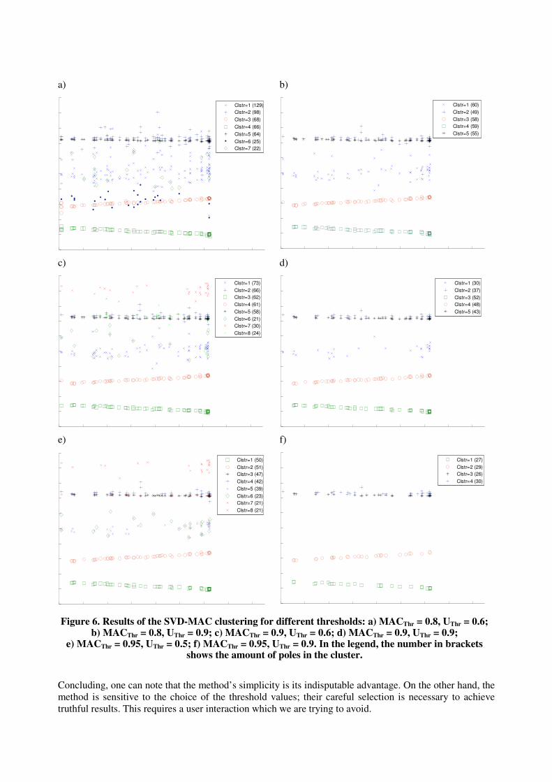
As it follows from the description of the steps, the technique is controlled by only two parameters: MAC

threshold MACThr (step 3) and singular vector threshold UThr (step 4c). Figure 6 presents the resulting

Campbell diagrams produced with different combinations of the two thresholds. In total, 65 datasets were

used for analysis; clusters with number of poles fewer than 20 are discarded.

Apparently, it is not straightforward to choose the values of the thresholds which will produce reasonable

results. Selecting low threshold values leaves the diagram noisy. In contrast, too conservative values

remove most of the information from the MAC matrix and the singular vectors, which results in filtering

out poles from the weak modes.

There are few indicators that can assist in selecting appropriate threshold values: e.g., a pole appearing in

more than one cluster indicates that one of the threshold values is too low. The number of poles in clusters

should not exceed the number of datasets used in the analysis (65 for the case presented in Figure 6).

Based on these indicators, one may argue that thresholds corresponding to Figure 6c and 6e lead to

expected results although in both of them few poles appeared in more than one cluster.

a)

8 9 10 11 12 13 14 15 16

Clstr=1 (129)

Clstr=2 (98)

Clstr=3 (68)

Clstr=4 (66)

Clstr=5 (64)

Clstr=6 (25)

Clstr=7 (22)

b)

8 9 10 11 12 13 14 15 16

Clstr=1 (60)

Clstr=2 (49)

Clstr=3 (58)

Clstr=4 (59)

Clstr=5 (55)

c)

8 9 10 11 12 13 14 15 16

Clstr=1 (73)

Clstr=2 (66)

Clstr=3 (62)

Clstr=4 (61)

Clstr=5 (58)

Clstr=6 (21)

Clstr=7 (30)

Clstr=8 (24)

d)

8 9 10 11 12 13 14 15 16

Clstr=1 (30)

Clstr=2 (37)

Clstr=3 (52)

Clstr=4 (48)

Clstr=5 (43)

e)

8 9 10 11 12 13 14 15 16

Clstr=1 (50)

Clstr=2 (51)

Clstr=3 (47)

Clstr=4 (42)

Clstr=5 (39)

Clstr=6 (23)

Clstr=7 (21)

Clstr=8 (21)

f)

8 9 10 11 12 13 14 15 16

Clstr=1 (27)

Clstr=2 (29)

Clstr=3 (26)

Clstr=4 (30)

Figure 6. Results of the SVD-MAC clustering for different thresholds: a) MACThr = 0.8, UThr = 0.6; b) MACThr = 0.8, UThr = 0.9; c) MACThr = 0.9, UThr = 0.6; d) MACThr = 0.9, UThr = 0.9;

e) MACThr = 0.95, UThr = 0.5; f) MACThr = 0.95, UThr = 0.9. In the legend, the number in brackets shows the amount of poles in the cluster.

Concluding, one can note that the method’s simplicity is its indisputable advantage. On the other hand, the

method is sensitive to the choice of the threshold values; their careful selection is necessary to achieve

truthful results. This requires a user interaction which we are trying to avoid.

5 Method Based on Self-Organizing Map

Self-Organizing Map (SOM) defines a projection of high-dimensional input data to a regular low-

dimensional (typically, two-dimensional) grid. SOM tries to preserve topological properties of the input

space: the items which are close to each other in the input space will be mapped to closely located items in

the output space. This property makes SOM useful for visualizing high-dimensional data on a low-

dimensional view (in other words, providing a multidimensional scaling). SOM was first described as a

type of artificial neural network trained using unsupervised learning by Tuevo Kohonen [12] (thus SOM is

sometimes called a Kohonen map). Since SOM is a general classification and multidimensional scaling

technique, its applications can be found in many areas e.g., medicine [13], stock market analysis [14],

geography and demographics [15], etc.

This article does not present the theory and algorithms behind SOM, they can be found in dedicated

literature. Several implementations of SOM are available; the implementation provided by the SOM

Toolbox for MATLAB [16] was used here.

As mentioned above, the input to SOM is high-dimensional data which need to be classified. In our case,

these are mode shape vectors associated with the poles resulting from application of OMA-SSI to different

datasets measured at different wind speed (Figure 2a): [{ψ1}…{ψN}], {ψj} ϵ CM

, where N is the number of

poles and M is a number of measured degrees-of-freedom; in the considered case, N = 1292 and M = 48.

Results of SOM are typically shown as so-called U-matrix, where the distances between the map items are

visualized by means of colors. Figure 7 shows a map resulting from the processing of the abovementioned

dataset. The ‘cold’ colors correspond to the smaller distances and the ‘hot’– to the bigger ones.

Visually analyzing the U-matrix, it is possible to imagine some clusters, the “cold”-colored areas isolated

from each other by “hotter” borders. Ovals in Figure 7 show manually identified clusters; the poles whose

projections belong to same clusters are believed to represent the same structural mode, while the poles

which are not inside any of the clusters are computational or noise modes.

However, the manual cluster identification is subjective and does not fulfill the requirement of minimal

user interaction for the ideal autonomous system: the automatic clustering technique is needed. This can

be achieved by using for example, a k-means clustering. K-means clustering is one of the techniques

known in data mining, which tries to partition the observations into a number of clusters so as to minimize

the within-cluster sum of distances. The theoretical background and the algorithm details are not within

the scope of this article and can be found in special literature. We used the k-means clustering algorithm

provided by the SOM Toolbox. The implementation uses a heuristic algorithm, which after a reasonable

computation time converges to a local optimum. Figure 8a presents an example of the clustering of the

SOM shown in Figure 7.

Unfortunately, the straightforward application of K-means clustering does not solve the problem of

filtering the computational and noise poles out. Figure 8b shows the Campbell diagram obtained from the

clusters in Figure 8a, where the poles belonging to different clusters are denoted by different symbols.

Comparing with Figure 2a, one can conclude that the diagram contains the same poles though they are

grouped now.

The essential properties of k-means clustering are responsible for this behavior of the algorithm; the

algorithm was originally designed for classification of noise-free data, and the number of clusters should

be set as an input parameter. Since a local optimum is found during the algorithm’s run, the results of

different runs might be different (Figure 9 shows an example). This can actually be utilized to improve the

abilities of the algorithm to deal with noisy data. It was noticed that clusters corresponding to structural

poles are relatively persistent and appear in the results of all runs while the clusters containing the noise

and computational poles change their amount and shape from run to run. Thus an “averaging” of several

runs will retain the wanted clusters and average out those which vary the most. The result of averaging

thirty k-means clustering runs is presented in Figure 10a. The big grey-colored area is where the not-

persistent clusters were. The poles corresponding to this area are considered as computational and noise

ones and they are being ignored when plotting the Campbell diagram. The corresponding Campbell

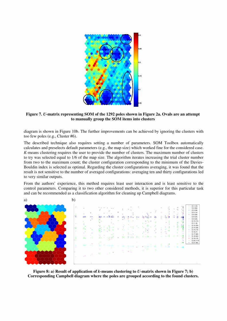
diagram is shown in Figure 10b. The further improvements can be achieved by ignoring the clusters with

too few poles (e.g., Cluster #6).

The described technique also requires setting a number of parameters. SOM Toolbox automatically

calculates and preselects default parameters (e.g., the map size) which worked fine for the considered case.

K-means clustering requires the user to provide the number of clusters. The maximum number of clusters

to try was selected equal to 1/6 of the map size. The algorithm iterates increasing the trial cluster number

from two to the maximum count; the cluster configuration corresponding to the minimum of the Davies-

Bouldin index is selected as optimal. Regarding the cluster configurations averaging, it was found that the

result is not sensitive to the number of averaged configurations: averaging ten and thirty configurations led

to very similar outputs.

From the authors’ experience, this method requires least user interaction and is least sensitive to the

control parameters. Comparing it to two other considered methods, it is superior for this particular task

and can be recommended as a classification algorithm for cleaning up Campbell diagrams.

a)

b)

Figure 8: a) Result of application of k-means clustering to U-matrix shown in Figure 7; b) Corresponding Campbell diagram where the poles are grouped according to the found clusters.

0.05

0.1

0.15

0.2

0.25

0.3

0.05

0.1

0.15

0.2

0.25

0.3

Figure 7. U-matrix representing SOM of the 1292 poles shown in Figure 2a. Ovals are an attempt

to manually group the SOM items into clusters

8 9 10 11 12 13 14 15

Cl.1 (13)

Cl.2 (64)

Cl.3 (36)

Cl.5 (14)

Cl.6 (55)

Cl.8 (34)

Cl.9 (22)

Cl.10 (12)

Cl.11 (8)

Cl.12 (33)

Cl.14 (39)

Cl.15 (14)

Cl.16 (7)

Cl.17 (65)

Cl.18 (64)

Cl.19 (15)

Cl.20 (113)

Cl.21 (90)

Figure 9. Results of four runs of the k-means clustering

6 Conclusion

The study presents and compares three methods aimed at cleaning up an experimentally obtained

Campbell diagram – a diagram showing a dependency of modal frequencies from the rotor speed. The

methods are demonstrated in application to the Campbell diagram of the lowest global modes of an

operational 3 MW wind turbine.

The main comparison criterion of the methods is their robustness; the main idea is to find a method which

fits the best model-based autonomous structure health monitoring system. The method shall require as

little user interaction as possible, shall have few controlling parameters and shall not be very sensitive to

these parameters.

All three methods, though very different, are known in data mining. The first method utilizes hierarchical

clustering and uses the dendrogram for clustering; the second method is based on singular value

decomposition of AutoMAC matrix, and the third one uses a self-organized map and averaged k-means

clustering to separate physical modes from computational and noise modes, group the former and discard

the latter.

a)

b)

Figure 10: a) Result of averaging of 30 runs of clustering algorithm; b) Corresponding Campbell diagram.

8 9 10 11 12 13 14 15

Cl.1 (75)

Cl.2 (64)

Cl.3 (63)

Cl.5 (63)

Cl.6 (8)

Cl.7 (39)

Cl.8 (55)

Cl.9 (20)

27 clusters25 clusters19 clusters23 clusters

The SVD based method (method number two) is the simplest one from the implementation view point; it

is controlled by only two parameters. However, it was found difficult to find a combination of the control

parameters which led to satisfactory results. The method is also sensitive to both control parameters: a

slight change in one of them has a great effect on the results.

The method based on hierarchical clustering (method number one) produces correct results and has only

one control parameter. However the method requires a lot of user interaction, which is comparable to the

SVD-based method. The implementation of the dendrogram software demonstrated low performance from

both computational speed and size of the input data point of view. However, the method led to correct

results and can be recommended for example to research tasks which do allow user interaction.

The method based on SOM (method number three) showed its superiority over the other two methods.

The method is controlled by a large number of parameters, but there are algorithms for automatic selection

of their default values. The main drawback of the method is due to some essential properties of the k-

means clustering; possibly a utilization of a different clustering technique can improve the method. This

could be a subject of future research. In the current study this drawback was overcome by using averaging,

which proved to be robust at the cost of increasing computational time.

In conclusion, the SOM-based method is believed to be the best candidate for a modal-based SHM system

among the considered methods.

Acknowledgements

The authors would like to thank Glenn Pietila for the idea of using SOM in this application and valuable

discussions during the project.

References

[1] C.-W. Lee, Vibration Analysis of Rotors, Kluwer Academic Publishers (2010).

[2] M. H. Hansen, Aeroelastic Instability Problems for Wind Turbines, Wind Energy 10, p.551-577,

(2007).

[3] C. E. Carcangiu, D. Tcherniak, S. Chauhan, J. Basurko, M. Rossetti, Numerical and Experimental

Modal Characterization of a 3MW Wind Turbine, Scientific Proceedings of European Wind Energy

Association, Copenhagen, Denmark (2012).

[4] A. W. Phillips, R. J. Allemang, D. L. Brown, Autonomous Modal Parameter Estimation:

Methodology, Proceedings of the 29th International Modal Analysis Conference, Jacksonville,

Florida, USA (2011).

[5] F. Magalhães, A. Cunha, E. Caetano, Permanent monitoring of “Infante D. Henrique” bridge based

on FDD and SSI-COV method, Proceedings of International Seminar on Modal Analysis, Leuven,

Belgium (2008).

[6] D. Tcherniak, S. Chauhan, M. H. Hansen, Applicability Limits of Operational Modal Analysis to

Operational Wind Turbines. Proceedings of the 28th International Modal Analysis Conference,

Jacksonville, Florida, USA (2010).

[7] D. Tcherniak, J. Basurko, O. Salgado, I. Urresti, S. Chauhan, C. E. Carcangiu, M. Rossetti,

Application of OMA to Operational Wind Turbine, Proceedings of 4th International Operational

Modal Analysis Conference, Istanbul, Turkey (2011).

[8] S. Chauhan, D. Tcherniak, J. Basurko, O. Salgado, I. Urresti, C. E. Carcangiu, M. Rossetti,

Operational Modal Analysis of Operating Wind Turbines: Application to Measured Data.

Proceedings of the 29th International Modal Analysis Conference, Jacksonville, Florida, USA (2011).

[9] D. J. Ewins, Modal Testing: Theory, Practice and Applications, Research Studies Press Ltd.,

Baldock, Hertfordshire, England (2000).

[10] A. Fernández, S. Gómez, Solving Non-uniqueness in Agglomerative Hierarchical Clustering Using

Multidendrograms. Journal of Classification 25, p.43-65, (2008).

[11] S. Chauhan, D. Tcherniak, Clustering Approaches to Automatic Modal Parameter Estimation,

Proceedings of the 27th International Modal Analysis Conference, Orlando, Florida, USA (2009).

[12] T. Kohonen, Self-organized formation of topologically correct feature maps. Biological Cybernetics,

43, p. 59-69, (1982).

[13] C. Thang, K. Kamei, D. T. Linh, Visualization System of Herbal Prescription Effects in Oriental

Medicine by Self-Organizing Map, Journal of Biomedical Fuzzy and Human Sciences, 14,(1), pp.101-108

(2009).

[14] H. V. Pham, C. Thang, E. W. Cooper, K. Kamei, Hybrid Kansei-SOM Model using Risk Management and

Company Assessment for Stock Trading, Information Sciences, Elsevier (Accepted), (2012).

[15] E. L. Koua, Using Self-organizing Maps for Information Visualization and Knowledge Discovery in

Complex Geospatial Datasets, Cartographic Renaissance, ICC 2003, p. 1694-1701, Durban, South

Africa (2003).

[16] J. Vesanto, J. Himberg, E. Alhoniemi, J. Parhankangas, SOM Toolbox for Matlab 5, Report A57,

Helsinki University of Technology, (2000).