Application of Machine Learning Techniques in ProjectManagement Tools

Miguel Ferreira de Sá Pedroso

Dissertation submitted to obtain the Master Degree in

Information Systems and Computer Engineering

Supervisor: Prof. Andreas Miroslaus Wichert

Examination Committee

Chairperson: Prof. Nuno João Neves MamedeSupervisor: Prof. Andreas Miroslaus Wichert

Member of the Committee: Prof. João Carlos Serrenho Dias Pereira

May 2017

ii

Acknowledgments

I would like to express my sincere gratitude to everyone that helped me during these years in my aca-

demic experience, for their patience, motivation and enthusiasm. A special thank you to my thesis

supervisor, Dr. Andreas Wichert.

iii

iv

Abstract

Nowadays, it is more important than ever to be as efficient as possible in order to overcome the diffi-

culties brought by the financial crisis and the economic deceleration that has been striking the western

countries. The high rates of project failure due to poor project planning hold back teams and potential

wealth creation.

In order to assist project managers in planning their projects and assessing risks, we created a sys-

tem that helps project managers to predict potential risks when they are planning their project milestones

based on their own previous experiences. The system is divided into 3 components: the Web-based

platform, the database and the MachineLearning core. In order to achieve this goal, we applied several

Artificial Intelligence techniques.

It is of utmost importance that our system is able to start performing risk analysis and providing sug-

gestions to project managers as early as possible, with the minimum amount of information as possible

fed into the system. In order to do this, we explore the application of techniques such as Instance-based

learning, which is a family of machine learning algorithms that compares new problem instances with

instances that were previously observed during the training, instead of performing explicit generalization,

like other algorithms such as neural networks. We also tried other methods such as regression model

algorithms.

The results from our evaluation are quite reasonable and show that the learning algorithms work well

when tested against scenarios that are expected to happen in the real world.

Keywords: Project Management Software, Machine Learning, Instance-based learning, Re-

gression models

v

vi

Resumo

Actualmente e mais importante do que nunca ser-se o mais eficiente possıvel com o objectivo de ul-

trapassar as dificuldades decorrentes da crise financeira e da desaceleracao economica que os paıses

ocidentais tem enfrentado. A elevada frequencia de fracasso de projectos e devida a deficiente planea-

mento.

Para assistir os gestores de projectos no desenvolvimento de melhor planeamento e analise de

riscos, criamos um sistema com o objectivo de os apoiar na prevencao de potenciais problemas en-

quanto planeiam milestones. A plataforma faz as previsoes baseadas no historial passado de cada

gestor de projectos. O nosso sistema esta dividido em tres componentes: uma plataforma Web, uma

base de dados e um nucleo de Machine Learning. Para atingirmos os nossos objectivos recorremos a

multiplas tecnicas de Inteligencia Artificial.

E importante que a nossa plataforma comece a realizar analise de risco o mais cedo possıvel na

experiencia de utilizacao do gestor de projectos, e com o mınimo possıvel de informacao introduzida no

sistema. E com este objectivo que exploramos a aplicacao de tecnicas como Instance-based learning,

que consiste numa famılia de algoritmos de aprendizagem automatica que compara novas instancias

de problemas com instancias que foram observadas previamente durante o treino do algoritmo, em

vez de realizarem generalizacao explıcita como algoritmos tais como redes neuronais. Tambem ex-

perimentamos resolver o problema com modelos de regressao e construımos o nosso sistema com

cenarios realistas.

Palavras-chave: Software de Gestao de Projectos, Machine Learning, Instance-based learn-

ing, Modelos de Regressao

vii

viii

Contents

Acknowledgments iii

Abstract v

Resumo vii

List of Figures xi

List of Tables xiii

Acronyms xv

1 Introduction 1

1.1 Problem . . . . . . . . . . . . . . . . . . . . . . . . . . . . . . . . . . . . . . . . . . . . . . 2

1.2 Goals . . . . . . . . . . . . . . . . . . . . . . . . . . . . . . . . . . . . . . . . . . . . . . . 3

1.3 Outline . . . . . . . . . . . . . . . . . . . . . . . . . . . . . . . . . . . . . . . . . . . . . . . 3

2 Related Work 5

2.1 IT Project Management . . . . . . . . . . . . . . . . . . . . . . . . . . . . . . . . . . . . . 5

2.1.1 The Waterfall model . . . . . . . . . . . . . . . . . . . . . . . . . . . . . . . . . . . 5

2.1.2 Spiral model . . . . . . . . . . . . . . . . . . . . . . . . . . . . . . . . . . . . . . . 7

2.2 Software Tools for Project Management . . . . . . . . . . . . . . . . . . . . . . . . . . . . 9

2.2.1 Microsoft Project . . . . . . . . . . . . . . . . . . . . . . . . . . . . . . . . . . . . . 9

2.2.2 Trello . . . . . . . . . . . . . . . . . . . . . . . . . . . . . . . . . . . . . . . . . . . 9

2.3 Machine Learning and Project Management . . . . . . . . . . . . . . . . . . . . . . . . . . 9

2.3.1 Instance-based learning . . . . . . . . . . . . . . . . . . . . . . . . . . . . . . . . . 9

2.3.2 k-Nearest neighbors algorithm . . . . . . . . . . . . . . . . . . . . . . . . . . . . . 11

2.3.3 Distance-weighted nearest neighbor algorithm . . . . . . . . . . . . . . . . . . . . 12

2.3.4 The curse of dimensionality . . . . . . . . . . . . . . . . . . . . . . . . . . . . . . . 13

2.3.5 Feature-weighted nearest neighbor . . . . . . . . . . . . . . . . . . . . . . . . . . . 13

2.4 Regression models . . . . . . . . . . . . . . . . . . . . . . . . . . . . . . . . . . . . . . . . 14

2.4.1 Logistic regression . . . . . . . . . . . . . . . . . . . . . . . . . . . . . . . . . . . . 14

2.4.2 Stochastic Gradient Descent . . . . . . . . . . . . . . . . . . . . . . . . . . . . . . 16

ix

2.4.3 Model overfitting and underfitting . . . . . . . . . . . . . . . . . . . . . . . . . . . . 16

2.4.4 Dynamic Learning Rate . . . . . . . . . . . . . . . . . . . . . . . . . . . . . . . . . 16

2.4.5 Momentum . . . . . . . . . . . . . . . . . . . . . . . . . . . . . . . . . . . . . . . . 16

3 Adaptive Risk Analysis Tool 18

3.1 Problem Formulation . . . . . . . . . . . . . . . . . . . . . . . . . . . . . . . . . . . . . . . 18

3.2 Data Models . . . . . . . . . . . . . . . . . . . . . . . . . . . . . . . . . . . . . . . . . . . 18

3.3 Techniques Explored . . . . . . . . . . . . . . . . . . . . . . . . . . . . . . . . . . . . . . . 20

3.3.1 Feature representation . . . . . . . . . . . . . . . . . . . . . . . . . . . . . . . . . . 21

3.3.2 Learning algorithms . . . . . . . . . . . . . . . . . . . . . . . . . . . . . . . . . . . 21

3.3.3 Nearest neighbor algorithms . . . . . . . . . . . . . . . . . . . . . . . . . . . . . . 21

3.3.4 Regression models . . . . . . . . . . . . . . . . . . . . . . . . . . . . . . . . . . . . 23

3.3.5 Hybrid approach . . . . . . . . . . . . . . . . . . . . . . . . . . . . . . . . . . . . . 23

3.3.6 Penalizing older experiences . . . . . . . . . . . . . . . . . . . . . . . . . . . . . . 24

4 Architecture and Implementation 25

4.1 General Overview . . . . . . . . . . . . . . . . . . . . . . . . . . . . . . . . . . . . . . . . 25

4.2 Web Platform . . . . . . . . . . . . . . . . . . . . . . . . . . . . . . . . . . . . . . . . . . . 26

4.2.1 Implementation . . . . . . . . . . . . . . . . . . . . . . . . . . . . . . . . . . . . . . 26

4.3 Database . . . . . . . . . . . . . . . . . . . . . . . . . . . . . . . . . . . . . . . . . . . . . 28

4.3.1 Implementation . . . . . . . . . . . . . . . . . . . . . . . . . . . . . . . . . . . . . . 28

4.3.2 Model . . . . . . . . . . . . . . . . . . . . . . . . . . . . . . . . . . . . . . . . . . . 28

4.3.3 Database Management System . . . . . . . . . . . . . . . . . . . . . . . . . . . . 28

4.4 ProjManagerLearnerOpt . . . . . . . . . . . . . . . . . . . . . . . . . . . . . . . . . . . . . 29

4.4.1 Implementation . . . . . . . . . . . . . . . . . . . . . . . . . . . . . . . . . . . . . . 29

5 Evaluation 31

5.1 Evaluation Sets and Environment . . . . . . . . . . . . . . . . . . . . . . . . . . . . . . . . 31

5.1.1 Sample data . . . . . . . . . . . . . . . . . . . . . . . . . . . . . . . . . . . . . . . 32

5.2 Solution quality . . . . . . . . . . . . . . . . . . . . . . . . . . . . . . . . . . . . . . . . . . 32

5.2.1 Accuracy . . . . . . . . . . . . . . . . . . . . . . . . . . . . . . . . . . . . . . . . . 32

5.3 Extensibility of the solution . . . . . . . . . . . . . . . . . . . . . . . . . . . . . . . . . . . 33

6 Conclusions 34

6.1 Summary . . . . . . . . . . . . . . . . . . . . . . . . . . . . . . . . . . . . . . . . . . . . . 34

6.2 Achievements . . . . . . . . . . . . . . . . . . . . . . . . . . . . . . . . . . . . . . . . . . . 34

6.3 Future Work . . . . . . . . . . . . . . . . . . . . . . . . . . . . . . . . . . . . . . . . . . . . 35

Bibliography 38

x

List of Figures

1.1 Reasons why projects fail according to The Bull Survey (1998) . . . . . . . . . . . . . . . 2

2.1 Waterfall model . . . . . . . . . . . . . . . . . . . . . . . . . . . . . . . . . . . . . . . . . . 6

2.2 Spiral model (Boehm, 2000) . . . . . . . . . . . . . . . . . . . . . . . . . . . . . . . . . . . 8

2.3 A typical Microsoft Project screen, displaying a list of tasks on the left and a Gantt chart

on the right. Source: Wikipedia . . . . . . . . . . . . . . . . . . . . . . . . . . . . . . . . . 10

2.4 A screenshot of the Trello platform. It shows five different boards, each one with many

cards. Each card has users assigned to it. . . . . . . . . . . . . . . . . . . . . . . . . . . . 10

2.5 The sigmoid function is bounded between 0 and 1 and introduces a non-linearity into the

logistic regression. . . . . . . . . . . . . . . . . . . . . . . . . . . . . . . . . . . . . . . . . 15

3.1 UML representing the both data models . . . . . . . . . . . . . . . . . . . . . . . . . . . . 19

4.1 ProjManager architecture schema . . . . . . . . . . . . . . . . . . . . . . . . . . . . . . . 26

4.2 Screenshot of the web platform showing a project’s Gantt chart . . . . . . . . . . . . . . . 27

4.3 Screenshot of a UI modal that allows a user to update his/her task status in order to

provide feedback to the system of how the project’s progress is going. . . . . . . . . . . . 27

xi

xii

List of Tables

5.1 Description of the datasets to test our algorithms against different scenarios . . . . . . . . 32

5.2 Each row represents the features of a milestone that is computed from the database

records. For better clarity we omitted the histogram of task types. . . . . . . . . . . . . . . 32

5.3 Accuracy of each algorithm on each dataset . . . . . . . . . . . . . . . . . . . . . . . . . . 33

xiii

xiv

List of Acronyms

k-NN k-Nearest Neighbors

PM Project Manager

SGD Stochastic Gradient Descent

xv

xvi

Chapter 1

Introduction

During the second half of the 20th century the world went through an information revolution with the

invention and wide adoption of computers. The adoption of machines that can be programmed to per-

form a high number of complex mathematical operations in a very short time was able to increase the

productivity and communication and accelerate the world economic development.

At the end of the century, the adoption of the Internet as a global network for communications lead

to a huge growth of the IT jobs market due to the need of developing and integrating a growing number

of IT software projects.

According to The Bull Survey (1998) the main reasons why the IT projects fail are related to prob-

lems during project management. These reasons break down into the categories depicted in 1.1. Some

projects are not properly planned, for example by having an improper requirement definition and a poor

risk analysis. Risk analysis is a task of utmost importance that should be done from a very early stage

of the project. It is important to identify the probability of something going wrong during the course of the

project and if something actually goes wrong, the team needs to have a plan to deal with the situation.

When these situations occur while the project is in a later phase of development, the risks can some-

times make the whole project not viable and therefore it will need to be canceled, after a great amount

of time and resources have been invested.

To help overcoming these challenges I decided to study and create a platform to be used by teams

to help them to improve their project planning, management and control. This platform will learn each

user’s particular management and planning style to provide suggestions, identifying risks based on the

user’s previous history.

1

Figure 1.1: Reasons why projects fail according to The Bull Survey (1998)

1.1 Problem

A more specific description of the problem that this dissertation is intended to solve is helping the user

to improve his/hers project planning activities in order to avoid and mitigate risks.

If we logically divide a project into several milestones and each milestone into the several tasks that

are necessary to complete it, then the technical problem that we really want to solve is the one that

consists on identifying similar milestone instances. If we model a solution where a milestone can have

zero or more problems / occurrences associated with itself, every time a project manager is planning a

new milestone using our system, we can look at his/hers work history and find similar milestones and

check them in order to perform risk analysis on the milestone that he/she is currently planning.

This is an interesting problem, as it must be solved in real-world scenarios and take human factors

into account (for example, that a project manager learns over time and tends not to repeat the same

mistakes indefinitely).

A possible solution to this problem will be carefully studied for the rest of this document, as we

consider it as being essential for us to build a system that is able to learn with the behavioral patterns of

the project manager and his/hers team, and assist them during their planning in order to maximize their

2

success and mitigate potential risks.

1.2 Goals

This thesis aims to solve the problem of high project failure rates due to bad or inadequate planning.

In order for this tool to be useful, deployed and adopted in real-world scenarios, the machine learning

algorithms must return solutions in real-time or near-real-time, and it must be integrated into a pleasant

and easy-to-use graphical user interface. To complete our goal, we must extensively analyze the existing

scientific work in the machine learning field and adapt it to our problem.

1.3 Outline

This document is organized as follows:

• Chapter 2 describes the related work about the subject of this thesis;

• Chapter 3 details important aspects of the problem, as well as the theoretical description of the

techniques used;

• Chapter 4 describes the system components and the architecture of the system as well as the

implementation choices and the chosen technologies;

• Chapter 5 details the evaluation tests that were made as well as the corresponding results;

• Chapter 6 summarizes the work developed and the future work.

3

4

Chapter 2

Related Work

In this thesis we address the problem of IT project failure due to poor planning and bad risk analysis.

In this chapter we review both project management methods and machine learning techniques and

applications.

2.1 IT Project Management

Project Management is defined as a discipline that has the goal of initiating, planning, executing, con-

trolling, and closing (Project Management Institute, 2004) the work of a team which has the goal of

achieving a certain predefined success criteria. A Project can be defined as being an individual or col-

laborative endeavor that is planned to achieve a particular aim. On the other hand, a Project Manager

is an individual that has the responsibility of planning and executing a particular project.

In the following sub-sections some of the popular project design processes will be presented in

detail. Despite the fact that project management is a general discipline, we will keep our focus in project

management techniques applied to IT projects.

2.1.1 The Waterfall model

The waterfall model (Royce, 1970) is a sequential project design process where the project orderly pro-

gresses through a sequence of defined steps beginning in the product concept or requirements analysis

to the system testing. The waterfall model usually serves as a basis for more complex and effective

project life-cycle models. Figure 2.1 shows an example Waterfall model with six phases.

The number of phases or steps in the waterfall model is flexible and depends on what the project

is and how the project manager wants to organize the project’s development; however the traditional

waterfall model usually features the 5 following phases:

• Requirement analysis - The project manager conferences with all the project’s stakeholders and

5

Figure 2.1: Waterfall model

the project’s team and gathers all the requirements in a requirement specification document.

• Design - The requirements of the project are carefully studied by the project’s team and the

project’s architecture is planned.

• Implementation - The development team starts to implement the software based on the design

obtained from the previous phase. The software is divided into small units. After the development

of all the units is completed, they are all integrated.

• Verification - In the verification phase, the software is properly tested against the project’s require-

ments and use cases.

• Maintenance - This phase consists on making small changes in the software to adapt it to possible

changes of the requirements that arose during the previous phases.

The biggest disadvantage of the waterfall model is that it is usually very hard to fully specify the

project requirements in the beginning of the project before any design or development has been per-

formed.

The person or organization that ordered the development of the project doesn’t always know from

the early stage of the problem what they really want to be build. Non-technical users and organizations

always plan to start a project with the goal of solving at least one problem but some of the requirements

to achieve that goal are very often only fully discovered during the design or development of the actual

6

project.

Despite of the previously pointed disadvantages, the waterfall model works quite well as a life-cycle

model in projects that are well understood from a technical point of view and that have a stable require-

ments definition since the beginning of the project planning (McConnell, 1996).

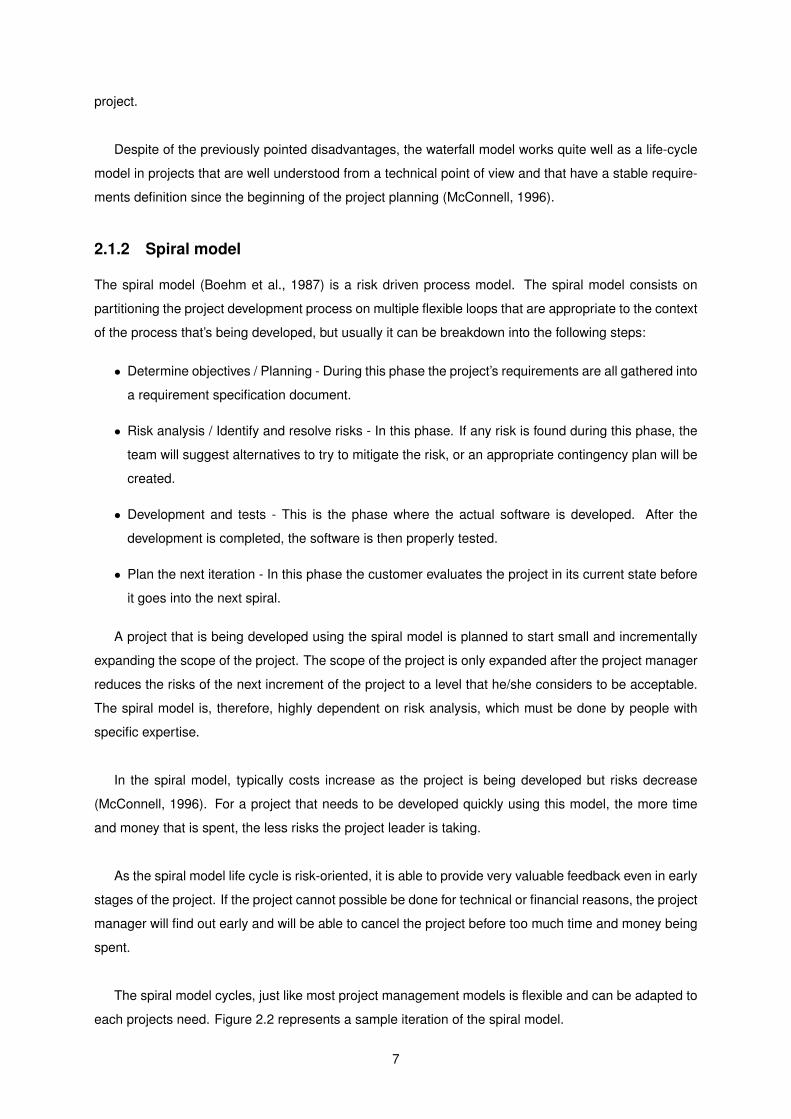
2.1.2 Spiral model

The spiral model (Boehm et al., 1987) is a risk driven process model. The spiral model consists on

partitioning the project development process on multiple flexible loops that are appropriate to the context

of the process that’s being developed, but usually it can be breakdown into the following steps:

• Determine objectives / Planning - During this phase the project’s requirements are all gathered into

a requirement specification document.

• Risk analysis / Identify and resolve risks - In this phase. If any risk is found during this phase, the

team will suggest alternatives to try to mitigate the risk, or an appropriate contingency plan will be

created.

• Development and tests - This is the phase where the actual software is developed. After the

development is completed, the software is then properly tested.

• Plan the next iteration - In this phase the customer evaluates the project in its current state before

it goes into the next spiral.

A project that is being developed using the spiral model is planned to start small and incrementally

expanding the scope of the project. The scope of the project is only expanded after the project manager

reduces the risks of the next increment of the project to a level that he/she considers to be acceptable.

The spiral model is, therefore, highly dependent on risk analysis, which must be done by people with

specific expertise.

In the spiral model, typically costs increase as the project is being developed but risks decrease

(McConnell, 1996). For a project that needs to be developed quickly using this model, the more time

and money that is spent, the less risks the project leader is taking.

As the spiral model life cycle is risk-oriented, it is able to provide very valuable feedback even in early

stages of the project. If the project cannot possible be done for technical or financial reasons, the project

manager will find out early and will be able to cancel the project before too much time and money being

spent.

The spiral model cycles, just like most project management models is flexible and can be adapted to

each projects need. Figure 2.2 represents a sample iteration of the spiral model.

7

Figure 2.2: Spiral model (Boehm, 2000)

8

2.2 Software Tools for Project Management

There are currently many software tools on the market that have the goal of helping project managers to

plan their projects, organize tasks, perform risk assessment and other related features. Some of these

tools will be briefly described in the following sub-sections. Even though there is a considerable amount

of good project management software, most of these tools do not offer any kind of ”machine learning”

solutions to assist the users.

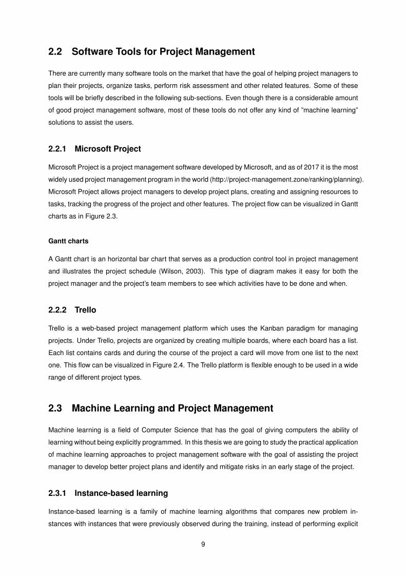
2.2.1 Microsoft Project

Microsoft Project is a project management software developed by Microsoft, and as of 2017 it is the most

widely used project management program in the world (http://project-management.zone/ranking/planning).

Microsoft Project allows project managers to develop project plans, creating and assigning resources to

tasks, tracking the progress of the project and other features. The project flow can be visualized in Gantt

charts as in Figure 2.3.

Gantt charts

A Gantt chart is an horizontal bar chart that serves as a production control tool in project management

and illustrates the project schedule (Wilson, 2003). This type of diagram makes it easy for both the

project manager and the project’s team members to see which activities have to be done and when.

2.2.2 Trello

Trello is a web-based project management platform which uses the Kanban paradigm for managing

projects. Under Trello, projects are organized by creating multiple boards, where each board has a list.

Each list contains cards and during the course of the project a card will move from one list to the next

one. This flow can be visualized in Figure 2.4. The Trello platform is flexible enough to be used in a wide

range of different project types.

2.3 Machine Learning and Project Management

Machine learning is a field of Computer Science that has the goal of giving computers the ability of

learning without being explicitly programmed. In this thesis we are going to study the practical application

of machine learning approaches to project management software with the goal of assisting the project

manager to develop better project plans and identify and mitigate risks in an early stage of the project.

2.3.1 Instance-based learning

Instance-based learning is a family of machine learning algorithms that compares new problem in-

stances with instances that were previously observed during the training, instead of performing explicit

9

Figure 2.3: A typical Microsoft Project screen, displaying a list of tasks on the left and a Gantt chart onthe right. Source: Wikipedia

Figure 2.4: A screenshot of the Trello platform. It shows five different boards, each one with many cards.Each card has users assigned to it.

10

generalization, like other algorithms such as neural networks (Aha et al., 1991).

On our particular domain, we want our system to learn each individual user patterns, and provide

information that will guide him/her over the course of his/her project management activities. In other

common types of machine learning a lot of data is collected to be used to train a learning model, like

logistic regression or artificial neural networks. These models learn an explicit representation of the

training data and then can be used to classify the training examples. The problem with this approach is

that it requires a considerable amount of training data, whereas in our practical domain, we want to help

the user of our system by providing suggestions or identifying project risks as early as possible. The

suggestions and risk analysis are dependent on each user and project type, so in our domain it is not

appropriate to construct a single large dataset for the entire platform. The user-dependent information

on the system is what must be used to provide information to that particular user. It is for this particular

reason that instance-based learning must be explored on our system, as it is able to perform machine

learning on a small and dynamically growing amount of data.

2.3.2 k-Nearest neighbors algorithm

The k-Nearest Neighbors (k-NN) algorithm (Altman, 1992) is a very simple instance-based learning

algorithm where each training example is defined as a vector in RN and is stored in a list of training

examples, every time it is observed. All the computation involved in classification is delayed until the

system receives a classification query. A query consists on either performing classification or regression

to the query point.

• Classification – The output of the algorithm is an integer that denotes the class membership of the

majority of the input point k-nearest neighbors.

• Regression – The output of the algorithm is a real-value number y that is the average of the values

of the k-nearest training examples to the input query point.

The common distance metric used in the k-NN algorithm is the Euclidean distance:

d(x1, x2) =

√√√√ n∑r=1

(ar(x1)− ar(x2))2

where x1 and x2 are two data points in Rn and ar(x) denotes the values of the rth coordinate of the

x data point.

Another distance metric that can be used and does not depend on the magnitude of the vector is the

cosine distance. The cosine similarity consists on the cosine of the angle between two points x1 and x2

and it is a value between −1 and 1. When the cosine is equal to 1 it means total similarity, when it’s 0 it

means that the vectors are orthogonal and when it’s −1 it means that they are exactly the opposite.

11

similarity(x1, x2) = cos(θ) =x1 · x2‖x1‖‖x2‖

The cosine similarity is, however, not a distance metric. It can be converted to a distance metric by

using the following expression:

d(x1, x2) =cos−1(similarity(x1, x2))

pi

Training a k-NN model can be done using Algorithm 1 and k-NN classification can be performed with

Algorithm 2.

Algorithm 1 k-NN Training algorithm1: procedure TRAIN2: Let Dexamples be a list of training examples3: For each training example (x, f(x)), add the example to the list Dexamples

Algorithm 2 k-NN Classification algorithm1: procedure CLASSIFY2: Let xq be a query instance3: Let x1 . . . xk be the k instances from the training-examples nearest to xq by a distance metric D4: Return f(xq) := argmax

∑ki=1 f(xi)

2.3.3 Distance-weighted nearest neighbor algorithm

The k-nearest neighbor algorithm can be modified to weight the contribution of each one of the query

points xq, by giving greater weight to close neighbors rather than distant ones. Clearly when classifying

a query point with the k-NN algorithm with k = 5, if 3 of the 5 nearest neighbors are clustered very

far from the query point xq and from its 2 other different neighbors, it may introduce noisy error to the

classification of the point.

By weighting the contribution of each point according to the distance we are considerably reducing

this problem. For example, the weight w of each stored data point i can be calculated with the expression

bellow that consists on the inverse square distance between the query point and each of the data points.

wi =1

d(xq, xi)2

with d denoting the selected distance metric.

With this tweak to the k-NN algorithm, the classification algorithm doesn’t even need to search for the

k-nearest neighbors of the query point as the inverse-square weight distance function almost eliminates

their contributions, so it is now appropriate to perform classification by using the contribution of the entire

stored training set.

12

2.3.4 The curse of dimensionality

Dealing with data points in an high-dimensionality hyperspace brings certain difficulties to nearest neigh-

bor search algorithms. For example, let x Rn with n = 50 be a vector where each coordinate represents

one of the 50 features available in that specific domain. Lets suppose that we want to perform a classi-

fication task on that dataset, but only 3 of the 50 dimensions of the vector are actually relevant for our

classification. While the 3 dimensions that represent features relevant to the classification could form

clusters of objects of the same category (eg. the vectors of the points of the same category are near

in space according to some distance metric d), the other 47 dimensions could make these points of

the same class becoming very far away, rendering the nearest neighbor algorithm completely useless,

without previous data processing.

This problem is called the ”curse of dimensionality” (Bellman, 2003) and occurs due to the fact that

there is an exponential increase in volume when adding extra dimensions through a mathematical space.

The standard implementation of the k-NN algorithm can therefore be rendered useless on vector

spaces with an high number of dimensions. In this case, the main problem stops being to find the

k nearest neighbors of the queries that are passed through the algorithm but to find a ”good” distance

function that is able to capture the similarity of two feature vectors where each feature will have a different

weight contribution to the distance function, based on the importance of that feature on the context of

the problem itself.

2.3.5 Feature-weighted nearest neighbor

One of the ways of overcoming the curse of dimensionality problem is by weighting the contribution of

each feature (Inza et al., 2002; Tahir et al., 2007), when performing k-nearest neighbor search. The

feature vector is composed with a meaningful representation of an instance of an individual model, but

not all the features have the same importance in each specific classification or regression problem. In

fact, some of the selected features may even be found to be irrelevant for a particular problem.

For example, the following equation can be used to calculate the feature-weighted euclidean distance

between two feature vectors.

d(x1, x2) =

√√√√ n∑r=1

(ar(wr.x1)− ar(wr.x2))2

where wr denotes the weight of the r feature, in the feature vectors.

13

2.4 Regression models

2.4.1 Logistic regression

Logistic regression is a regression model where the dependent variable (i.e. the variable that represents

the output value of the model) is categorical (Freedman, 2005). Logistic regression can either have a

binomial dependent variable (in the case where there are only two target categories), or multinomial

(when there are more than two categories).

The goal of Logistic regression is to create a model that receives an input vector x (eg. a vector

that represents a real-world object) and outputs an estimate y. The following expression can be used to

calculate the prediction of a given logistic regression model.

y = σ(Wx+ b) (2.1)

σ =1

1 + e−z(2.2)

The output of a logistic regression model consists on the weighted average of the inputs passed

through a sigmoid activation function. The weights W and the bias term b are the parameters of the

model that need to be learned. If the non-linear activation function was not used, then logistic regres-

sion would be the same as linear regression (Zou et al., 2003). The sigmoid function σ is bounded

between 0 and 1 and is a simple way of introducing a non-linearity into the model and conveying a more

complex behavior.

In order to train the regression model (i.e. finding the desired values for the parameters W and b),

we can employ numerical optimization techniques such as Stochastic Gradient Descent (SGD) (Ruder,

2016).

Regression can be used not only to train a model that is able to make predictions, but can also be

used to weight the contribution of each feature in the feature vector for a particular problem. The magni-

tude of each learned parameter in binomial logistic regression does not directly represent the ”semantic

importance” of the particular feature that the parameter is associated to, in the context of the problem

that’s being modeled. For example, the feature vector f of dimension n could have one feature that

represents the mere scaling of another feature (eg: f1 = 100f0). In this case, the learned coefficients

associated with those features, would be different by a factor of about 100, while at the same time, the

semantic importance of features f0 and f1 would be the same.

However, at the same time, the model will tend to learn smaller coefficients that are associated

with less important feature vectors. As an example, if feature f3 consists of random noise and has no

semantic importance in the classification problem whatsoever, as long as the model converges during

14

Figure 2.5: The sigmoid function is bounded between 0 and 1 and introduces a non-linearity into thelogistic regression.

training time, a small coefficient will be learned so that the noisy feature gets filtered out.

Cost function

A cost function (also called a loss function) is a function C used in numerical optimization problems, that

returns a real scalar number which represents how well a model performs to map training examples into

the correct output.

The Binary cross-entropy function is a way of comparing the difference between two probability

distributions t and o and is usually used as the cost function of binary logistic regression (when the

output of the logistic regression if a scalar binary value - 0 or 1).

crossentropy(t, o) = −(t.log(o) + (1− t).log(1− o)) (2.3)

where t is the target value and o is the output predicted by the model.

When the logistic regression algorithm is used to classify data into multiple categories, the categorical

cross-entropy function is usually used as the loss function.

H(p, q) = −∑

p(x)log(q(x)) (2.4)

where p is the true distribution and q is the coded distribution (the one that results from the models

predictions at any given moment in time).

15

2.4.2 Stochastic Gradient Descent

Gradient descent is a first order numerical optimization algorithm that is commonly used to train differen-

tiable models (Ruder, 2016). A model can be trained by defining a cost function which can be minimized

by using the Gradient Descent algorithm, that updates the model parameters on each time-step, by

applying the following rule:

θ := θ − η δδθJ(θ) (2.5)

where η is the learning rate and θ is the parameter that is going to be learned and J is the cost

function.

This rule is applied iteratively and changes the value of the parameter until the model converges into

a local minima of the cost function.

Wij := Wij − ηδ

δWijJ(W, b) (2.6)

bi := bi − ηδ

δbiJ(W, b) (2.7)

where W is a weight matrix and b is a bias term.

2.4.3 Model overfitting and underfitting

In a statistical model, overfitting is the term used to describe the noise or the random error that is part

of the model, rather than the true underlying relationship between the input vector and the output value.

Overfitting usually occurs when the model is either ”too big” or the training data that is passed to the

training algorithm is not enough.

2.4.4 Dynamic Learning Rate

It is a common practice to decay the learning rate during the training process, just like the Simulated

Annealing (Kirkpatrick and Gelatt, 1983) algorithm. The following rule, if applied at each training epoch

t, will exponentially decay the learning rate:

ηt+1 := rηt (2.8)

where r is a constant that denotes the decay ratio of the learning rate at each epoch.

2.4.5 Momentum

When the standard gradient descent algorithm is minimizing the cost function, the hyperspace topology

of the model may have a shape of a ravine with steep walls, and the gradient updates will tend to oscillate

16

between both the walls of the ravine. This situation can become a problem while training deep neural

network models, as it can considerably slow down the training, or even cause divergence of the model.

In order to overcome this issue we can store the updates for all the parameters at it time-step, and in

the next step, the update will be a combination of the current gradient with the latest update. By doing

this we are able to avoid abrupt changes in the direction of the updates, usually leading to a faster

convergence of the model (Sutskever et al., 2013). The following expression (2.9) is the rule to update

the parameter weights in SGD with momentum:

W(l)ij (t) := W

(l)ij (t)− η δ

δW(l)ij

J(W, b) + α∆W(l)ij (t− 1) (2.9)

where W(l)ij (t) and α is a coefficient (between 0 and 1) that controls the amount of momentum that’s

applied to the training.

When training with momentum, it is also common to change dynamically the α momentum scale

coefficient. By starting with a small momentum coefficient we allow the initial parameter updates to

be fast. Then, after a few training epochs, usually we need the network to converge and have smaller

steps, thus increasing the momentum coefficient will resist the abrupt changes and allows the model to

converge.

αt+1 := rαt (2.10)

where r is a constant that denotes the rate at which the momentum coefficient will change at each

epoch.

17

Chapter 3

Adaptive Risk Analysis Tool

Before we describe our system, we need to explain in detail what is the problem we address, which

parameters we have to consider, and, which restrictions/constraints we have to take into account. The

following sections describe the problem, the relevant data to the problem and how it is organized, as well

as the explored techniques.

3.1 Problem Formulation

Our problem consists on performing risk analysis at the ”milestone” level. In order to perform risk analysis

on a particular milestone that is being planned at a certain point in time, we must find similar milestones

in the project manager previous history and check its registered problem occurrences.

3.2 Data Models

In order to create a solution that helps teams to manage their projects by providing suggestions and

identifying risks based on each user previous history requires storing information in several appropriate

data models. The structure of these models and their purpose will be described bellow.

A Project is divided into Milestones and each Milestone is divided into Tasks. These three data

models store the information necessary to keep track of the structure of the projects in our platform. A

milestone can be independent from all the others, but can also be connected to another milestone that

must have been completed previously.

Figure 3.1 shows a UML representation of both data models that were detailed in the following

subsections.

• Project:

– ID

18

Figure 3.1: UML representing the both data models

– Name

– Start Date

– Due Date

• Milestone:

– ID

– Name

– Project (FK)

– Previous Milestone (FK)

– Type

– Start Date

– Due Date

• Task:

– ID

– Name

– Project (FK)

– Milestone (FK)

– Type

– Expected Duration

– Due Date

19

– Status

– Complete Date

We also need to have models that will store the feedback from the user throughout the project. The

ProblemOccurrence model has the purpose of storing problems that any team member may experience

during the project, while the ChangeEstimate model has the purpose of keeping track of the changes in

the duration of tasks made by the project manager or by any user assigned to that task.

• Problem:

– ID

– Name

• ProblemOccurrence:

– ID

– Problem (FK)

– Milestone (FK)

– Task (FK)

– Date

• ChangeEstimate:

– ID

– Milestone (FK)

– Task (FK)

– Date

– Old Estimate

– New Estimate

3.3 Techniques Explored

In this Section, we provide a description of the techniques used to develop a solution to the problem of

creating a machine learning approach to help project managers to plan their projects.

As we want to perform a risk analysis per milestone, we need to compare the current milestone which

is being planned by the project manager with previous milestones that are stored in the system. In order

to do this, we must list the features that will be used to create a feature vector for each milestone.

• Features of each Milestone:

– Number of Users

20

– Number of Tasks

– Duration

– Type

– Average duration of tasks

– Duration of the Project

– Order of the Milestone in the Project

– Standard deviation of the duration of the tasks

– Histogram of the Task types

3.3.1 Feature representation

The Type of a milestone is a categorical feature which can be any value c in the set of milestone types

LMilestoneTypes. Let l = {A,B,C,D} be the list of milestone types of a particular project manager. With-

out any prior information of similarities between types, we must assume that all the types are equally

different to each other. If we choose to represent each category as it’s index in the list (a single integer

value), we run into problems while using distance metrics such as the euclidean distance, as the dis-

tance between the type A and type B and lower than the distance between type A and type D.

In order to address this issue, the milestone Type feature can be represented as a one-hot vector,

which is a vector that has zero magnitude in all its directions but one, where the magnitude will be equal

to 1. This vector v ∈ Rn will where k is the number of categories. The vector will have magnitude 1 in

the dimension that corresponds to the index of the Type in the set of possible milestone types.

As an example, to represent the type C ⊂ s we use the following one-hot vector:

FType =

0

0

1

0

(3.1)

3.3.2 Learning algorithms

In order to solve our problem, we use two types of machine learning algorithms: Instance-based learning

algorithms and Regression models.

3.3.3 Nearest neighbor algorithms

One of the approaches used to solve our problem is using nearest neighbor search in order to find

similar milestones and perform risk analysis during the planning of the current project.

21

Top milestone risks

The output of the nearest neighbor algorithm consists on the k-nearest neighbors to the query point. In

our domain, the nearest neighbor are milestone vectors. We check if the milestones associated with

these vectors have any problem occurrences associated. From our data models, problem occurrences

are associated with individual tasks. As a milestone is composed of multiple tasks, a milestone can have

a problem of a certain type associated with itself multiple times. If so, we then will check what is the

most common problem associated with that milestone.

Representing Problem Occurrences

As our system is designed to be an open web platform used by many project managers working at the

same time and we need to provide user-specific suggestions, we needed to have a way of representing

the problem occurrences in our algorithms. In a real-world scenario a wide variety of problem types may

occur during the course of a project. We represent problem types as an integer. An integer number

represents the index of a problem in the user-specific problems list. For example, if a user experienced

problems of type A, B and C in his/her past history then the problem-integer mapping will become

{A : 0, B : 1, C : 2}.

Feature selection and weighting

Nearest neighbor algorithms such as the k-NN can sometimes face the curse of dimensionality problem

where on particular scenarios only a few features in the feature vector are meaningful to the partic-

ular problem in hand. In our domain, a project manager may plan a project and only face project

management-related problems on certain kinds of milestones, like milestones of a certain ”duration” in

time (i.e. short milestones). In our vectorial representation, the ”duration” of the milestone is represented

as one dimension in the vector space, while at the same time, the rest of the vector will represent fea-

tures that are not really relevant in this particular scenario.

In order to solve this problem I propose a regression-based feature selection, where a coefficient will

be assigned to each feature. This coefficient represents ”how important” the feature is to a particular

user. Large coefficients will reinforce the importance of a particular feature in the feature vector and

a smaller coefficient will reduce the importance of the feature. This technique can be thought off as

expanding and contracting the vector space in order to manipulate the nearest neighbor search.

As each project manager user has his/her own work history and experiences, feature weighting must

be done individually for each project manager. To do this we create a training set that consists on a list of

the milestone vectors that are stored in the system and were planned by that particular project manager.

The logistic regression model is trained using the SGD algorithm with momentum and converges

in real time in real-world scenarios as the number of stored milestones of each project manager is

22

usually small enough for this computation to be quick. In our current application of the logistic regression

algorithm, we are not interested on the model’s predictions but rather on the learned parameters wr.

Each parameter wr will serve as the ”importance” coefficient for the r dimension of the milestone vector.

3.3.4 Regression models

We also tried an alternative approach to the nearest neighbor algorithms by building a logistic regression

model that is able to predict a potential project risk from an input milestone (i.e. the milestone that a

project manager as just introduced into the system). In order to do this we build a training set T consist-

ing on (x, y) tuples where x is a milestone vector and y an integer that represents the problem instance

that occurred when the project team was working on that particular milestone.

The probability of each problem type happening can be calculated with the expression 3.2:

P (Y = i|x,W, b) = softmaxi(Wx+ b) =eWix+bi∑j e

Wjx+bj(3.2)

A softmax activation function is used as it is a generalization of the logistic function used in multi-

categorical classification (Bishop, 2006). The top risk can be predicted with he following expression:

ypred = argmaxi(P (Y = i|x,W, b)) (3.3)

The model is then trained using the SGD algorithm with momentum and is able to predict risks in

a simple manner. This logistic regression model differs from the one used in the previous subsection

due to the fact that we are now performing multi-categorical classification instead of just classifying if an

input milestone has a potential risk or not.

The model learns how to predict a risk from an input milestone but the model itself results from global

optimization so it has no longer information about every single training example. This is a limitation of this

type of technique in contrast to instance-based learning methods where all the information is stored and

on particular scenarios may provide better information to the project manager (i.e. when two problems

occurred during the course of a particular past milestone and can now occur again but the model does

not have the information to predict it).

3.3.5 Hybrid approach

Another interesting way of approaching our problem is to provide an hybrid solution that uses both

instance-based learning and regression models. Even though in regression models we no longer can

access the user’s past experiences, we are still able to predict the top risk associated with an input

milestone vector.

23

An hybrid solution may consist on building a table of potential risks returned from the output of both

algorithms and weight the contribution of each algorithm on the all risks. The top risk will be the one with

the greatest contribution.

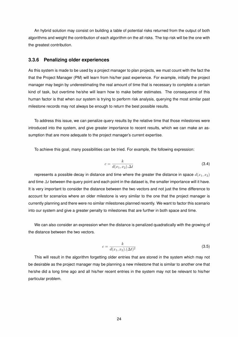
3.3.6 Penalizing older experiences

As this system is made to be used by a project manager to plan projects, we must count with the fact the

that the Project Manager (PM) will learn from his/her past experience. For example, initially the project

manager may begin by underestimating the real amount of time that is necessary to complete a certain

kind of task, but overtime he/she will learn how to make better estimates. The consequence of this

human factor is that when our system is trying to perform risk analysis, querying the most similar past

milestone records may not always be enough to return the best possible results.

To address this issue, we can penalize query results by the relative time that those milestones were

introduced into the system, and give greater importance to recent results, which we can make an as-

sumption that are more adequate to the project manager’s current expertise.

To achieve this goal, many possibilities can be tried. For example, the following expression:

c =k

d(x1, x2).∆t(3.4)

represents a possible decay in distance and time where the greater the distance in space d(x1, x2)

and time ∆t between the query point and each point in the dataset is, the smaller importance will it have.

It is very important to consider the distance between the two vectors and not just the time difference to

account for scenarios where an older milestone is very similar to the one that the project manager is

currently planning and there were no similar milestones planned recently. We want to factor this scenario

into our system and give a greater penalty to milestones that are further in both space and time.

We can also consider an expression when the distance is penalized quadratically with the growing of

the distance between the two vectors.

c =k

d(x1, x2).(∆t)2(3.5)

This will result in the algorithm forgetting older entries that are stored in the system which may not

be desirable as the project manager may be planning a new milestone that is similar to another one that

he/she did a long time ago and all his/her recent entries in the system may not be relevant to his/her

particular problem.

24

Chapter 4

Architecture and Implementation

In this chapter, the details about the architecture used in our solution will be described. The system was

built with the goal of being versatile and easily modified, so that this work can be expanded in the future

by introducing new modules that may help to improve this solution and turn it into a even more valuable

system.

To implement the all features discussed in this chapter, some decisions were made about the pro-

gramming languages, platforms and tools that were used. Our goal was to utilize cross-platform, open-

source and well documented solutions to implement our system, to make it portable, scalable and highly-

reliable.

The following sections will also describe the choices that were made about the implementation of our

platform.

4.1 General Overview

Our system is divided into three main independent components as in shown Figure 4.1:

• Web Platform - it is used by the end users (project managers) to manage their projects, introduce

information and get feedback;

• Database - it has the purpose of storing all the data in a persistent way;

• ProjManagerLearnerOpt - the module that is responsible to handle all the queries that require

responses based on machine learning.

The arrows in Figure 4.1 represent data flows between the components. The interactions with the

database are read/write actions, but the interaction between the web platform and the software to gen-

erate the solution is just an activation interaction. In this case, the platform starts the software; however,

the result is written in the database and not directly returned to the web platform.

25

Web Platform

Database

ProjMngLearnerOpt

Figure 4.1: ProjManager architecture schema

In the following sections, we present the details for the web platform as well as for the software

responsible for the machine learning. The database component is used just to store data. There is no

logic associated with this component.

4.2 Web Platform

After considering multiple options it was decided that the system would run in a web platform. A web

platform makes it possible for its users to access it from everywhere in the world, and with any device

with a web browser, including mobile devices. It is important that a system that has the goal of helping

teams managing their projects has also an interface that can be accessed very easily.

• User

1. Create, Change and Delete Projects

2. Create, Change and Delete Milestones

3. Create, Change and Delete Tasks

4. Report Occurrence (associated with a Task)

Figure 4.3 is a screenshot of one screen of the web platform. This page shows a Gantt chart, which

is the main UI component of the platform and is used to represent the project’s planned flow.

4.2.1 Implementation

The web platform was developed by using the Django framework, which is an high-level web framework

that follows the model-view-template (MVT) design pattern (Burch, 2010). The reason why django was

chosen was because it is a simple but powerful open-source framework with a very big community; it

has exhaustive documentation and has a large amount of available plug-ins that can be used to extend

the platform. It also is cross-platform and supports many database management systems, including

PostgreSQL, MySQL and SQLite.

26

Figure 4.2: Screenshot of the web platform showing a project’s Gantt chart

Figure 4.3: Screenshot of a UI modal that allows a user to update his/her task status in order to providefeedback to the system of how the project’s progress is going.

27

The django framework is also cross-platform and django projects can be easily deployed to the most

common web servers, including Apache and Nginx.

As this platform’s goal is to help the teams to manage their projects it is of utmost importance to

provide a pleasant, straight-forward and good-looking user interface so that the end-users will actually

use this system. In order to respond to this requirement, the Twitter Bootstrap 1 HTML, CSS, and JS

framework. Bootstrap can be used to create UIs that are appealing to the users and that looks good on

a wide range of screen sizes, including on mobile devices.

4.3 Database

The database component is used to store information in a persistent and consistent way and has no

special features or functionalities. The web platform is connected to the database and reads and writes

data. The database is a key component of this platform as it is where all the data provided by the users

is stored.

4.3.1 Implementation

We do not have the need to use any particular platform-specific features to develop or deploy our so-

lution. We rather just need to use the basic database operations to access and manipulate the data:

Select, Insert, Update and Delete.

4.3.2 Model

This project uses a relational database as its storage system. There are currently many other possibil-

ities, but relational databases were chosen because they are widely used and they allow the practical

implementation of the models presented in Section 3.2 with minor changes. It is not the scope of this

dissertation to explore alternative methods to store information.

4.3.3 Database Management System

There are plenty of DBMS that implement a relational model. Despite having different features, all of

those DBMS have a common base. We are just interested in those base features. So our choice of

DBMS was based again in easy access to infrastructure.

To develop this platform we used SQLite which is a very lightweight database management system

and stores the information on a single small file on the OS file system, which makes it very portable.

SQLite has the advantage of not requiring any particular configurations or database server. On the other

hand SQLite has poor performance and does not support user management but these issues are not

1http://getbootstrap.com/

28

relevant during the development time. The DBMS chosen for the deployment of the platform is Post-

greSQL2.

Switching from this DBMS to another will not have any performance implications. There are no

complex queries that may take advantages from better query optimizers. All queries are basic with no

advanced operators.

4.4 ProjManagerLearnerOpt

The ProjManagerLearnerOpt component is used to perform all the machine learning operations of the

platform. This component is connected with both the database and the web platform. When a user

makes an operation that requires a machine learning response (for example, the user has just finished

to plan a project milestone, and wants to perform risk analysis on that particular milestone) the web

platform queries the ProjManagerLearnerOpt system which then makes database queries, computes

the result using the appropriate algorithms and returns the response to the web platform.

The reason why the ProjManagerLearnerOpt component is kept separated to the web platform (not

only in the system architecture, but also in the implementation itself) is to make it possible for the plat-

form to scale while on production. The web platform could itself do all the tasks that the ProjMan-

agerLearnerOpt component does, but we want to make sure that the machine learning component that

will perform all the heavy computation can easily be replicated into several servers, depending on the

amount of users using the platform at a particular point in time. In this scenario the web platform would

use a load balancer that would decide which ProjManagerLearnerOpt server is available to serve the

user’s requests.

4.4.1 Implementation

The ProjManagerLearnerOpt module was developed in the python language, just like the web platform

module. The reason for this choice is that python is one of the most used programming languages for

machine learning and data science, containing a great amount of highly optimized and actively main-

tained machine learning libraries, such as scikit-learn, Tensorflow, Theano, Pylearn2 and Caffe.

In this module we often need to perform many mathematical computations, and for that we use the

python’s NumPy library, which is the fundamental library for scientific computing in Python. As python

is an interpreted language, code runs slower than in other compiled programming languages such as C

and C++. In order to address this issue, the NumPy library has many of its operations implemented in

C, bringing must faster running times to python (van der Walt et al., 2011).

2https://www.postgresql.org/

29

Other libraries such as Tensorflow and Theano were also created to be very efficient (Abadi et al.,

2015; Theano Development Team, 2016). They work by allowing the developer to construct a compu-

tational graph of mathematical operations, which is then compiled and optimized for CPU and GPU.

This computational graph can be used to perform very complex functions, such as training deep neural

networks. The GPU offers significant performance improvement to the CPU in linear algebra operations

as matrix operations can be parallelized.

30

Chapter 5

Evaluation

In the previous chapters we described the architecture and inner workings of our solution that has the

goal of helping IT project managers to better plan their projects in order to prevent and mitigate any pos-

sible risks that may arise. It is, therefore, of utmost importance to assess the quality of the developed

solution by performing evaluation tests and take conclusions according to the obtained results.

In this chapter, we will evaluate and discuss our solution. We will also analyze the quality and

acceptance of the generated solutions.

5.1 Evaluation Sets and Environment

In order to evaluate our solution we programmatically created several datasets. The task of helping

project managers during the planning of their projects is dependent not only on the project type and fea-

tures, but on the project manager himself/herself. An inexperienced project manager can, for example,

underestimate the time that is necessary to complete a certain type of task and therefore create delays

in the delivery of a milestone, and thus, the project itself. As the learning task is dependent on the project

manager himself/herself, it is necessary to create datasets that have this situation into account.

The datasets consists on several lists of Projects, Milestones and tasks, where each milestone can

be associated with at least one Problem instance (that represents an occurrence that happened during

the course of that milestone). Each of these components, as described in chapter 3, has several defining

properties. Assigning random values to all the properties of the instances of these models would then

render the learning task impossible and useless. The properties of the milestones and tasks are as-

signed with values that are between intervals of realistic values. In order to make the dataset useful and

interesting, we introduce certain ”biases” into the dataset generator algorithm. For example, milestones

of type ”A” with more than ”n” tasks, have ”k%” probability of reporting the occurrence of problem of type

”P”.

31

Another important factor to consider while building the datasets is that project managers learn over

time. For example an inexperienced project manager that uses our platform may underestimate the time

needed to complete the milestones in the beginning, but may learn how to correctly estimate the dura-

tion over time. To address this real-life scenario, part of the evaluation sets are also generated taking

this into account.

Table 5.1 details the datasets used to evaluate our learning algorithms. These datasets are then

randomly divided into a training set and a validation set (on a 7:3 proportion, approximately).

Number of

projects

Number of

milestones

Number of

tasks

PM learns

over time

Dataset 1 1 16 100 No

Dataset 2 3 30 200 No

Dataset 3 3 30 200 Yes

Table 5.1: Description of the datasets to test our algorithms against different scenarios

5.1.1 Sample data

In Table 5.2 we present an example of a fragment of the training dataset:

# users # tasks Duration TypeAvg

Duration

Proj

DurationOrder

Std dev

of duration

Top

problem

1 5 10 30 A 6.1 122 0 5.72 X

2 2 4 5 A 6.25 122 4 2.21 Y

3 4 8 15 B 7.1 122 3 5.99 -

4 2 5 12 A 8.4 180 7 3.51 X

5 3 5 20 B 10.2 180 2 6.30 Z

Table 5.2: Each row represents the features of a milestone that is computed from the database records.

For better clarity we omitted the histogram of task types.

5.2 Solution quality

5.2.1 Accuracy

In Table 5.3, we present the accuracy of several applied techniques when used to predict the top po-

tential problem of a project’s milestone. The k-NN + TIME method is a k-NN classifier that gives more

importance to the latest history of the team rather than the old (unless the old records are much ”closer”

to the query point). The k-NN + FEATURE method consists on k-NN with feature weighting performed by

a logistic regression model. The LOGREG method consists on a logistic regression model that predicts

the top potential problem for the input milestone.

32

Dataset 1 Dataset 2 Dataset 3k-NN (k=3) 75% 83.33% 22.22%k-NN + FEATURE 100% 100% 33.33%k-NN + TIME 75% 83.33% 83.33%k-NN + FT + TIME 100% 100% 100%LOGREG 87.5% 100% 22.22%

Table 5.3: Accuracy of each algorithm on each dataset

From the results we obtained we observe that all the techniques used are learning and presenting

good results. The k-NN algorithm with feature weighting seems to perform very well when few data is

present, like in Dataset 1. Logistic regression models seem to perform decently, even though seem to

perform a little poorer when less training examples are available.

Logistic regression also performs poorly on datasets where the user learns over time, like we ex-

pected as it is trained with the entire user history, making it a little bit more inadequate in real-world

scenarios.

5.3 Extensibility of the solution

Another very important point of our solution, mainly on the web platform is the fact that it was designed

to be extended in a simple way. We employ a mechanism of connecting the web platform to our machine

learning back-end that is generic enough to be replaced by a different one with minimum amount of effort

from the developers.

33

Chapter 6

Conclusions

6.1 Summary

In this dissertation we proposed a system that has the goal of helping project managers to improve their

planning by performing risk analysis based on their previous professional history, every time they are

planning a project milestone.

Our literature review showed that there are two main types of machine learning algorithms that con-

tribute to solve this problem: Instance-based learning and Regression models. We developed models

using both approaches. Our tests show that both techniques are able to give quite satisfiable results

when applied on real-world scenarios.

We were able to integrate these algorithmic solutions into a platform that can be used by project

managers and their teams in order to be more efficient and improve their project success rates by

discovering and mitigating potential risks before they happen.

6.2 Achievements

This work allowed us to develop a solution that project managers can use in order to prevent potential

risks based on their previous experience and work history. The evaluation of our work showed that the

machine learning algorithms are able to provide very satisfactory results, while dealing with different time

of human factors such as the fact that project managers tend to learn with their own mistakes overtime.

Our solution takes all these human factors into account with the goal of providing the best possible risk

analysis and prevention solution.

34

6.3 Future Work

We consider that our work can have several future improvements in order to achieve better results. One

of the ways we think it would be interesting to explore in the future, after this system is fully deployed

and used by many dozens of users on real-life scenarios, would be to study global patterns in the user’s

history. This could be achieved by applying machine learning algorithms (eg. clustering algorithms like

k-Means Clustering) to divide the users into several clusters. Each of these individual clusters would

represent project managers and teams with similar experiences and profiles.

We speculate that this could be very helpful when performing risk analysis on types of tasks and

milestones that a specific user never performed before. According to that user’s own profile, the system

could predict several potential project planning risks based on previous experiences from other users of

the platform with a similar profile and history.

35

36

Bibliography

Abadi, M., Agarwal, A., Barham, P., Brevdo, E., and Zhifeng Chen, e. a. (2015). TensorFlow: Large-scale

machine learning on heterogeneous systems. Software available from tensorflow.org.

Aha, D. W., Kibler, D., and Albert, M. K. (1991). Instance-based learning algorithms. Machine Learning,

6(1):37–66.

Altman, N. S. (1992). An introduction to kernel and nearest-neighbor nonparametric regression. The

American Statistician, 46:175–185.

Bellman, R. E. (2003). Dynamic Programming. Dover Publications, Incorporated.

Bishop, C. M. (2006). Pattern Recognition and Machine Learning (Information Science and Statistics).

Springer-Verlag New York, Inc., Secaucus, NJ, USA.

Boehm, B. W., Defense, T. R. W., Group, S., Boehm, H. W., Defense, T. R. W., and Group, S.

(1987). A Spiral Model of Software Development and Enhancement. Computer (Long. Beach. Calif).,

21(May):61–72.

Burch, C. (2010). Django, a web framework using python: Tutorial presentation. J. Comput. Sci. Coll.,

25(5):154–155.

Freedman, D. (2005). Statistical models: theory and practice.

Inza, I., Larranaga, P., and Sierra, B. (2002). Feature Weighting for Nearest Neighbor by Estimation of

Distribution Algorithms, pages 295–311. Springer US, Boston, MA.

Kirkpatrick, S. and Gelatt, J. R. (1983). Optimization by simulated annealing.

McConnell, S. (1996). Rapid Development: Taming Wild Software Schedules. Microsoft Press, Red-

mond, WA, USA, 1st edition.

Project Management Institute (2004). A Guide To The Project Management Body Of Knowledge (PM-

BOK Guides). Project Management Institute.

Royce, W. (1970). Managing the development of large software systems. Proceedings of IEEE

WESCON.

Ruder, S. (2016). An overview of gradient descent optimization algorithms. Web Page, pages 1–12.

37

Sutskever, I., Martens, J., Dahl, G. E., and Hinton, G. E. (2013). On the importance of initialization and

momentum in deep learning. Jmlr W&Cp, 28(2010):1139–1147.

Tahir, M. A., Bouridane, A., and Kurugollu, F. (2007). Simultaneous feature selection and feature weight-

ing using hybrid tabu search/k-nearest neighbor classifier. Pattern Recognition Letters, 28(4):438 –

446.

The Bull Survey (1998). The bull survey. London: Spikes Cavell Research Company.

Theano Development Team (2016). Theano: A Python framework for fast computation of mathematical

expressions. arXiv e-prints, abs/1605.02688.

van der Walt, S., Colbert, S. C., and Varoquaux, G. (2011). The numpy array: a structure for efficient

numerical computation. CoRR, abs/1102.1523.

Wilson, J. M. (2003). Gantt charts: A centenary appreciation. European Journal of Operational Re-

search, 149(2):430 – 437. Sequencing and Scheduling.

Zou, K. H., Tuncali, K., and Silverman, S. G. (2003). Correlation and simple linear regression. Radiology,

227(3):617–628.

38