application of inﬂow control devices to heterogeneous ...aib29/icd_het_ecmor_xii.pdf ·...

Application of Inflow Control Devices to HeterogeneousReservoirs

Birchenko, V. M.Institute of Petroleum Engineering

Heriot–Watt UniversityEdinburgh, EH14 4AS, U.K.

[email protected]

Bejan, A. Iu.Computer Laboratory

University of Cambridge15 J.J. Thomson Ave., Cambridge, CB3 0FD, UK

[email protected]

Usnich, A. V.Institut fur Mathematik

Universitat Zurich190 Winterthurerstr., 8057 Zurich, Switzerland

[email protected]

Davies, D. R.Institute of Petroleum Engineering

Heriot–Watt UniversityEdinburgh, EH14 4AS, U.K.

[email protected]

Abstract

The rate of inflow to a long well can vary along its completion length, e.g. due to frictionalpressure losses or reservoir heterogeneity. These variations often negatively affect the oil sweepefficiency and the ultimate oil recovery. Inflow Control Devices (ICDs) represent a mature wellcompletion technology which provides uniformity of the inflow profile by restricting high specificinflow segments while increasing inflow from low productivity segments. This paper introduces amathematical model for effective reduction of the inflow imbalance caused by reservoir heterogene-ity. The model addresses one of the key questions of the ICD technology application—the trade-offbetween well productivity and inflow equalisation. Our analytical model relates the specific inflowrate and specific productivity index to well characteristics, in marked contrast to the numerical na-ture of existing, simulation-based models. Our model takes into account the intrinsically stochasticnature of reservoir properties along the well completion interval. A general solution to our model isavailable in a non-closed, analytical form. We have derived a closed form solution for some particu-lar cases. The practical utility of the model is illustrated by considering a case study with prolific andmedium productivity reservoirs. Finally, we identify certain limitations of using our model. Theserefer to cases when (i) annular flows can be neither neglected nor eliminated, and (ii) the neglectof frictional pressure losses is not a valid assumption, that is when both reservoir heterogeneity andfriction have substantial impact on the inflow distribution.

Keywords: Inflow Control Devices, ICD, equalisation, heterogeneity

ECMOR XII – 12th European Conference on the Mathematics of Oil Recovery, 6 – 9 September 2010, Oxford, UK

Andrei Bejan

Typewritten Text

Introduction

Increasing well-reservoir contact has a number of potential advantages in terms of well productivity,drainage area, sweep efficiency and delayed water or gas breakthrough. However, such long, possiblymultilateral wells bring not only advantages but also present new challenges in terms of drilling, com-pletion and production. One of these challenges is that the variation in rock properties (and hence fluidspecific inflow rate) tends to increase with increasing well length. Completion intervals with a lengthof several thousands of feet have become very popular in the last few years. Such completions willoften have significantly uneven specific inflow distribution along their length if special measures are nottaken. These inflow variations often cause premature water or gas breakthrough and, hence, should beminimised.

Advanced well completions have proved to be a practical solution to this challenge. Inflow ControlDevices (ICDs) and Interval Control Valves (ICVs) are two established types of advanced completions.ICVs permit an active control of inflow (or outflow) of multiple completion intervals or laterals (Gai,2002), while ICDs provide a passive form of inflow control (Birchenko et al., 2008).

ICDs have been installed in hundreds of wells during the last decade and are now considered to be amature well completion technology. The steady-state performance of ICDs can be analysed in detailwith well modelling software (Ouyang and Huang, 2005; Johansen and Khoriakov, 2007). Most reser-voir simulators include basic functionality for ICD modelling while some of them (Wan et al., 2008;Neylon et al., 2009) also offer a practical means to capture the effect of annular flow. Current numericalsimulation software provide engineers with the tools to perform the design and economic justification ofan ICD completion. However, relatively simple analytical models still have a role to play in:

• Quick feasibility studies (screening ICD installation candidates).

• Verification of numerical simulation results.

• Communicating best practices in a non-product specific manner.

This paper proposes an analytical model for heterogeneous reservoirs that quantifies the reduction ofinflow variation along a horizontal well with ICDs installed. This model allows one to estimate:

• The ICD design parameters that substantially reduce the inflow variation caused by reservoir het-erogeneity.

• The impact of a specific ICD completion on Inflow Performance Relationship (IPR) of a long wellcompleted in a heterogeneous reservoir.

Assumptions

Our model invokes the following assumptions with respect to the inflow from the reservoir:

• Flow through the reservoir can be described by Darcy’s law.

• Steady or pseudo-steady state flow into the well.

• The distance between the well and the reservoir boundary is much longer than the well length (orthe boundary is parallel to the well).

• The perpendicular-to-the-well components of the reservoir pressure gradients are much greaterthan the along-hole ones.

ECMOR XII – 12th European Conference on the Mathematics of Oil Recovery6 – 9 September 2010, Oxford, UK

The above simplifications are often introduced in analytical descriptions of coupling of reservoir andwellbore flow. They are required to introduce the notion of “specific productivity index” (PI per unitlength). This empirical parameter indicates that the fluid inflow from reservoir to wellbore is propor-tional to the pressure difference between the external reservoir boundary and the annulus:

dq

dl= j(l)(Pe(l)− Pa(l)). (1)

The chosen assumptions for the description of the wellbore flow are that:

• Friction and acceleration pressure losses between the toe and the heel are small compared to thedrawdown. Conditions under which this assumption is valid are discussed in Birchenko et al.(2010).

• The fluid is incompressible.

Note that we do not assume the completion interval to be perfectly horizontal. The true vertical depth(TVD) can vary along the completion. Reservoir pressure at the external boundary, Pe, is measured atthe same TVD as the corresponding point l of the tubing.

The above assumptions imply that the difference between the reservoir pressure Pe and the tubing pres-sure P is constant throughout the completion length:

Pe(l)− P (l) = ∆Pw = const. (2)

Our assumptions about the ICDs are as follows:

1. There is no flow in the annulus parallel to the base pipe, i.e. the fluid flows from reservoir directlythrough ICD screens into the base pipe.

2. ICDs of the same “strength” are installed throughout the completion length.

3. The flow distribution along the wellbore’s internal flow conduit q(l) is “smooth” (i.e. it has acontinuous derivative).

These assumptions were previously discussed in more detail by Birchenko et al. (2009). The reader isreferred to Section Nomenclature at the end of this paper for complete nomenclature.

Problem Formulation

Let us analyse the impact of an ICD completion on the well inflow profile when the well is completedin a heterogeneous reservoir. The specific inflow rate is the derivative of the flow rate with respect to themeasured depth. We designate a separate notation U to this quantity since it is central to this paper:

U(l) ≡ dq(l)

dl. (3)

The Specific Productivity Index, j, and hence the inflow, U , change stochastically along the completioninterval. We will use a coefficient of variation to quantify the degree of these changes. Recall that thecoefficient of variation of a random variable is defined as the ratio of its standard deviation and its mean.


The annulus pressure Pa is equal to the base pipe pressure P for a conventional completion (no ICD).Hence

U(l) = j(l)∆Pw, (4)

where ∆Pw is a constant independent of l. Eq. (4) shows that, in case of conventional completion (noICD), the coefficient of variation of specific inflow is equal to that of the specific PI:

CoVU = CoV j. (5)

ICD application reduces the variation of inflow so that

CoVU < CoV j. (6)

Inequality (6) may seem intuitively obvious to engineers familiar with the ICD technology, however itsrigorous mathematical proof known to the authors is not straightforward (see the proof at the end of thepaper).

Let us consider the ratio of the two coefficients of variation, CoVU/CoV j. This ratio equals unity fora conventional completion and decreases monotonically with increasing ICD strength. The magnitudeof this decrease is a quantitative measure of the equalisation of the inflow along the completion lengthdue to the ICD. The objective of this work is to develop a mathematical model linking the ratio of thetwo coefficient of variations with well parameters (such as ICD “strength”, drawdown, etc.)

Solution

Birchenko et al. (2009) presented the following solution for the inflow to an ICD well:

U(l) =−1 +

√1 + 4a∆P (l)j2(l)

2aj(l), (7)

qw =

∫ L

0

−1 +√

1 + 4a∆P (l)j2(l)

2aj(l)dl, (8)

where

a =

(ρcal µρµcal

)1/4ρρcal

l2ICDB2aICD for channel ICD

an =Cuρl2ICDB

2

C2dd

4 for nozzle or orifice ICD.(9)

Formula (8) is of limited use for a “quick-look” analysis if the local specific productivity index variessubstantially along the completion interval since:

1. The exact shape of the productivity profile j(l) is often unknown:

• Detailed measurements (logging) are not always feasible.

• The productivity index changes with time (e.g. due to fluid saturation changes).

2. In general one needs to evaluate the integral (8) numerically even if j(l) is known (or can beestimated).

The engineering team that develops each well drilling proposal will normally define an expected rangeof values for the specific productivity index, j, as part of the proposal. These could be based on:

• Well log data.


• Reservoir models.

• Production performance of similar wells in the same field.

This range of values may take a number of forms. For instance, in its simplest form it could compriseof only three values: pessimistic (P90), most probable (P50) and optimistic (P10). Ideally, a completespecification of j would be available in the form of a probability density function (p.d.f.). In the casewhen j depends on some other parameters and information about their distribution is available thisdensity can be estimated, for example, via Monte-Carlo simulation.

It is often easier to describe the statistical distribution of the specific productivity index, η(j), rather thanits spatial distribution j(l). This allows us to transform formula (8) into

qw = L

∫ j2

j1

−1 +√

1 + 4a∆Pwj2

2ajη(j) dj. (10)

Calculation of the coefficient of variation requires mean and mean square values of the specific inflowrate. The mean specific inflow rate is the ratio of the well flow rate to its length:

〈U〉 = qw/L =

∫ j2

j1

−1 +√

1 + 4a∆Pwj2

2ajη(j) dj. (11)

Similarly, its mean square value is calculated as follows:

〈U2〉 =

∫ j2

j1

(−1 +

√1 + 4a∆Pwj2

2aj

)2

η(j) dj. (12)

The choice of the method for solving the integrals (11) and (12) depends on the functional form of η(j),the p.d.f. of the specific PI. Notably, these integrals can be solved analytically for a piecewise linear p.d.f.(e.g. a uniform or triangular distribution). The corresponding solutions are presented below. When thedensity function has a more complex form (e.g. a normal or log-normal distribution) the integrals can beevaluated numerically.

Uniform Distribution of Specific Productivity Index

Generally speaking, a uniform distribution of the specific productivity index is unlikely to be encoun-tered in practice. In fact, petro-physical quantities are usually modelled by a normal or log-normaldistribution. However, the data required to determine the distribution parameters with sufficient preci-sion is often unavailable. A uniform distribution may be a sensible starting assumption when data isscarce.

Assuming that j is uniformly distributed between two values j1 and j2, j1 ≤ j2, its density function isas follows:

η(j) =

{1/(j2 − j1) for j1 ≤ j ≤ j20 otherwise.

(13)

In this case:

qw = 〈U〉L =IU (j2)− IU (j1)

j2 − j1L, (14)

andCoVU

CoV j=

(j2 + j1)√

3 (〈U2〉 − 〈U〉2)〈U〉(j2 − j1)

, (15)


where

〈U2〉 =SU (j2)− SU (j1)

j2 − j1(16)

with

IU (j) =

√1 + 4a∆Pwj2 − ln

(1 +

√1 + 4a∆Pwj2

)2a

, (17)

SU (j) =1

2a2j

(−1 + 2a∆Pwj

2 +√

1 + 4a∆Pwj2−

−2j√a∆Pw arcsinh

(2j√a∆Pw

)).

(18)

Triangular Distribution of Specific Productivity Index

The most probable, or modal value is often known within reasonable error margins in addition to knowl-edge about the minimum and maximum values of the specific PI. The specific productivity index j maythen be modelled by the (more complex) triangular distribution. This is a legitimate approach if a trian-gular distribution can be fitted to the field data almost as well as more common normal or log-normaldistributions.

The p.d.f. of a triangular distribution is as follows:

η(j) =

2(j − j1)/(j2 − j1)/(jm − j1) for j1 ≤ j ≤ jm2(j2 − j)/(j2 − j1)/(j2 − jm) for jm ≤ j ≤ j20 otherwise.

(19)

Then

qw = 〈U〉L =2L

j2 − j1

(IUj(jm)− IUj(j1)− j1 (IU (jm)− IU (j1))

jm − j1+

+j2 (IU (j2)− IU (jm))− IUj(j2) + IUj(jm)

j2 − jm

), (20)

and

CoVU

CoV j=j2 + jm + j1〈U〉

√2 (〈U2〉 − 〈U〉2)

j21 + j22 + j2m − j1j2 − j1jm − j2jm, (21)

where

〈U2〉 =2

j2 − j1

(SUj(jm)− SUj(j1)− j1 (SU (jm)− SU (j1))

jm − j1+

+j2 (SU (j2)− SU (jm))− SUj(j2) + SUj(jm)

j2 − jm

)(22)

with

IUj =1

2a

(−j +

j√

1 + 4aj2∆Pw2

+arcsinh

(2j√a∆Pw

)4√a∆Pw

), (23)

SUj(j) =∆Pj2/2− IU (j)

a, (24)

and functions IU and SU defined by (17) and (18) respectively.


Case Study

This case study shows how our model for a uniform distribution can be used in practice for the followingtwo cases:

1. Prolific Reservoir

2. Medium Productivity Reservoir.

This case study quantitatively illustrates the dependence between the specific PI and ICD “strength”required to reduce inflow variations.

Prolific Reservoir

Let us consider a 1 km long well completed in a prolific heterogeneous reservoir (Table 2). The antici-pated PI of the well is 2 000 Sm3/day/bar. A drawdown, ∆Pr, of 0.5 bar is required for a conventionalcompletion to achieve the target well rate of 1 000 Sm3/day. Pressure drop introduced by conventionalcompletion is usually negligible compared to the drawdown:

∆Pw ≈ ∆Pr = 0.5 bar. (25)

The inflow distribution along the completion is expected to be highly uneven and uncertain due to com-plex reservoir geology. The local specific productivity index is anticipated to be within the range of0.5 - 3.5 Sm3/day/bar/m. Subject to the model assumptions stated earlier, the inflow to the conventionalcompletion will be proportional to the local specific productivity index. This implies a 7-fold variationof specific inflow rate for the above case.

A completion combining ICDs and annular flow isolation will improve oil recovery by smoothing outthe specific inflow rate variations and increasing oil sweep efficiency along the above horizontal well(Birchenko et al., 2008).

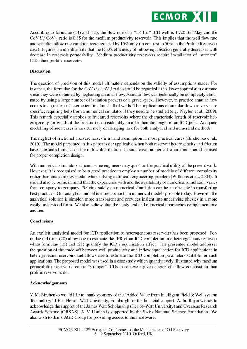
The uniform distribution model (formula (14)) predicts that “1.6 bar” ICD completion with ∆Pw of 1bar will produce 1 070 Sm3/day. That is, the “1.6 bar” ICD completion reduced well productivity byapproximately 50% (for the target rate), but also delivered an improved degree of inflow equalisation(Figure 3). The grey line in Figure 3 was obtained using formula (7). The specific inflow rate variationis considerably smaller than for a conventional completion. Namely, the CoVU/CoV j ratio of 0.52 forthe “1.6 bar” ICD case can be interpreted as almost a 50% reduction of the difference between regionsof high and low specific inflow rate.

An increase in the ICD strength gives an even more uniform inflow at the cost of further reduction ofwell inflow performance. This is illustrated in figures 4 and 5 which were derived using formulae (14)and (15) for ∆Pw = 1 bar.

Medium Productivity Reservoir

The specific productivity index is the key parameter in ICD completion design. The majority of ICDinstallations to date are in reservoirs with an average permeability of one Darcy or greater (Birchenkoet al., 2008). In order to illustrate the importance of this parameter let us now consider the case with 10times lower PI (200 Sm3/day/bar) and 10 times higher total pressure drop (10 bar). Such modifications(Table 3) would not change the inflow performance of conventional completion as it is the product ofthe PI and the pressure drop that determines the inflow rate. However, the performance of an ICDcompletion will be different since the inflow is no longer proportional to the above mentioned productin this case.


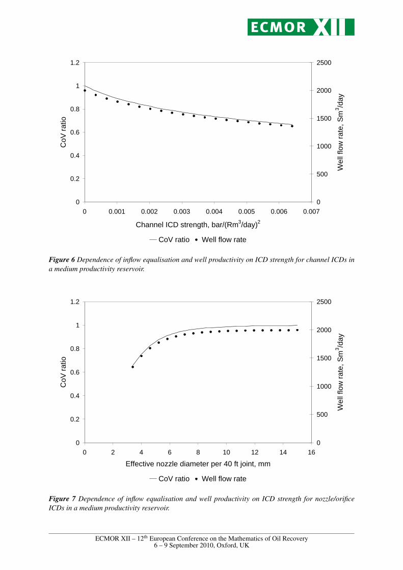
According to formulae (14) and (15), the flow rate of a “1.6 bar” ICD well is 1 720 Sm3/day and theCoVU/CoV j ratio is 0.85 for the medium productivity reservoir. This implies that the well flow rateand specific inflow rate variation were reduced by 15% only (in contrast to 50% in the Prolific Reservoircase). Figures 6 and 7 illustrate that the ICD’s efficiency of inflow equalisation generally decreases withdecrease in reservoir permeability. Medium productivity reservoirs require installation of “stronger”ICDs than prolific reservoirs.

Discussion

The question of precision of this model ultimately depends on the validity of assumptions made. Forinstance, the formulae for the CoVU/CoV j ratio should be regarded as its lower (optimistic) estimatesince they were obtained by neglecting annular flow. Annular flow can technically be completely elimi-nated by using a large number of isolation packers or a gravel-pack. However, in practice annular flowoccurs to a greater or lesser extent in almost all of wells. The implications of annular flow are very casespecific; requiring help from a numerical simulator if they need to be studied (e.g. Neylon et al., 2009).This remark especially applies to fractured reservoirs where the characteristic length of reservoir het-erogeneity (or width of the fracture) is considerably smaller than the length of an ICD joint. Adequatemodelling of such cases is an extremely challenging task for both analytical and numerical methods.

The neglect of frictional pressure losses is a valid assumption in most practical cases (Birchenko et al.,2010). The model presented in this paper is not applicable when both reservoir heterogeneity and frictionhave substantial impact on the inflow distribution. In such cases numerical simulation should be usedfor proper completion design.

With numerical simulators at hand, some engineers may question the practical utility of the present work.However, it is recognised to be a good practice to employ a number of models of different complexityrather than one complex model when solving a difficult engineering problem (Williams et al., 2004). Itshould also be borne in mind that the experience with and the availability of numerical simulation variesfrom company to company. Relying solely on numerical simulation can be an obstacle in transferringbest practices. Our analytical model is more coarse than numerical models possible today. However, theanalytical solution is simpler, more transparent and provides insight into underlying physics in a moreeasily understood form. We also believe that the analytical and numerical approaches complement oneanother.

Conclusions

An explicit analytical model for ICD application to heterogeneous reservoirs has been proposed. For-mulae (14) and (20) allow one to estimate the IPR of an ICD completion in a heterogeneous reservoirwhile formulae (15) and (21) quantify the ICD’s equalisation effect. The presented model addressesthe question of the trade-off between well productivity and inflow equalisation for ICD applications inheterogeneous reservoirs and allows one to estimate the ICD completion parameters suitable for suchapplications. The proposed model was used in a case study which quantitatively illustrated why mediumpermeability reservoirs require “stronger” ICDs to achieve a given degree of inflow equalisation thanprolific reservoirs do.

Acknowledgements

V. M. Birchenko would like to thank sponsors of the “Added Value from Intelligent Field & Well systemTechnology” JIP at Heriot–Watt University, Edinburgh for the financial support. A. Iu. Bejan wishes toacknowledge the support of the James Watt Scholarship (Heriot–Watt University) and Overseas ResearchAwards Scheme (ORSAS). A. V. Usnich is supported by the Swiss National Science Foundation. Wealso wish to thank AGR Group for providing access to their software.


Proof of the coefficient of variation ratio inequality

Formula (7) expresses the greatest root of the following quadratic equation:

aU2 + U/j −∆P = 0. (26)

Since all coefficients (a, 1/j and ∆P ) of the above equation are strictly positive and finite, its greatestroot is a positive real-valued random variable.

We use the transformation Y = U/√

∆P , X = j√

∆P to rewrite Eq. (26) as follows:

aY 2 + Y/X − 1 = 0. (27)

Since the applied transformation is linear, it preserves the coefficient of variation. Thus CoV Y =CoVU and CoVX = CoV j. It follows that the inequality (6) is identical to:

CoV Y < CoVX, (28)

where X and Y are positive random variables linked by Eq. (27). We will therefore prove the inequality(28) as means to prove (6).

We define a map y 7→ x as a continuous bijection

x =y

1− ay2(29)

from the interval (0, a−1/2) to (0,∞). We also define the following function:

F (a) =

∫∞0

(y

1−ay2

)2dh(y)(∫∞

0y

1−ay2 dh(y))2 ,

where h(y) is the probability density function of Y . It follows that:

F (0) =

∫∞0 y2 dh(y)(∫∞0 y dh(y)

)2 = 1 + CoV(Y )2,

F (a) =

∫∞0 x(y; a)2 dh(y)(∫∞0 x(y; a) dh(y)

)2 = 1 + CoV(X)2,

where x(y; a) is a parametric function defined by (29).

The following theorem proves that F (0) ≤ F (a) for any non-negative real value of a, and hence thatCoV(Y ) ≤ CoV(X). We also prove that equality is possible if and only if Y (and hence X) has adegenerate distribution.Theorem 1. The function F satisfies the inequality F (a) ≥ F (0) where, except for the case when a = 0,equality holds if and only if h is a point mass distribution.

Proof. We use the following notation Ik =∫∞0 yk dh(y) and develop the nominator and denominator

of F (a) as series in a exchanging sums and integrals since all integrals are absolutely convergent:∫y

1− ay2dh(y) =

∑n≥0

anI2n+1,

∫ (y

1− ay2

)2

dh(y) =∑n≥0

(n+ 1)anI2(n+1),(∫y

1− ay2

)2

dh(y) =∑n≥0

an∑

0≤m≤nI2m+1I2(n−m)+1.


Now the theorem will follow if we manage to prove that ∑0≤m≤n

I2m+1I2(n−m)+1

I2I21≤ (n+ 1)I2n+2,

where equality holds if and only if h represents a one-point mass distribution. The latter inequality,however, automatically follows from the following inequalities:

I2m+1I2(n−m)+1I2 ≤ I2n+2I21 , m = 0, . . . , n. (30)

In order to show (30) we use the Cauchy inequality(∫f(y)g(y) dh(y)

)2

≤∫f(y)2 dh(y)

∫g(y)2 dh(y),

where equality holds if and only if f is proportional to g almost everywhere (with respect to h and itssupport). In particular,

I2k ≤ Ik+1Ik−1. (31)

Since Y is a positive random variable and h is a proper probability density function (it integrates tounity) the case I2 = 0 is not possible. Hence I2 > 0, and (31) implies that Ik > 0 for all k. In thiscase the Cauchy inequality (31) takes the form of equality only when yk+1 is proportional to yk−1 onthe support of h. This implies that Y can take only one non-zero value almost surely, that is to say h isconcentrated on at most one point outside zero. We can rewrite (31) as follows:

I2I1≤ . . . ≤ Ik

Ik−1≤ Ik+1

Ik. (32)

In particular,I2I1≤ I2n+2

I2n+1, (33)

andI2m+1

I1≤ I2m+2

I2≤ I2m+3

I3≤ . . . ≤ I2n+1

I2(n−m)+1, (34)

so thatI2m+1

I1≤ I2n+1

I2(n−m)+1, m = 0, . . . , n. (35)

By multiplying the inequalities (33) and (35) we obtain the key inequality

I2m+1I2(n−m)+1I2 ≤ I2n+2I21 ,

which holds for any m = 0, . . . , n.

Thus the inequalities (30) are proven and the proof is complete.

Nomenclature

Fluid volumes are quoted at standard conditions (S) while fluid viscosity and density are in downhole(R) conditions.

B Formation volume factor

Cd Discharge coefficient for nozzle or orifice


Cu Unit conversion factor: 8/π2 in SI units, 1.0858 · 10−15 in metric units, 7.3668 · 10−13 infield units

IU (j) An auxiliary function, see equation (17), page 9

IUj(j) An auxiliary function, see equation (23), page 11

J Well’s productivity index

P Tubing (base pipe) pressure

Pa Annulus pressure

Pe(l) Reservoir pressure at the external boundary at the same TVD as point l of the wellbore)

Pw Flowing bottom hole pressure (at the heel of the tubing), i.e. P (L)

SU (j) An auxiliary function, see equation (18), page 10

SUj(j) An auxiliary function, see equation (24), page 11

U Inflow per unit length of completion

∆P Pressure difference between the external reservoir boundary and the tubing (base pipe).

∆Pr Pressure difference between the external reservoir boundary and the annulus, Pe − Pa

∆Pw Total pressure drop at the heel, Pe − Pw

arcsinh Inverse hyperbolic sine

η(j) Probability density function of the specific productivity index

〈〉 Angled brackets are used to denote average values of variables

µ Viscosity of produced or injected fluid

µcal Viscosity of calibration fluid (water)

ρ Density of produced or injected fluid

ρcal Density of calibration fluid (water)

aICD Channel ICD strength (Table 1)

d Effective diameter of nozzles or orifices in the ICD joint of length lICD

j1 Minimum value of specific productivity index

j2 Maximum value of specific productivity index

jm The mode (peak) of the triangular p.d.f.

l Distance between particular wellbore point and the toe

lICD Length of the ICD joint (typically 12 m or 40 ft)

q Flow rate in the tubing

qw Well flow rate q(L)

ICD Inflow Control Device


ICV Interval Control Valve

IPR Inflow Performance Relationship

p.d.f. Probability density function

PI Well Productivity Index

TVD True Vertical Depth

References

Birchenko, V., Al-Khelaiwi, F., Konopczynski, M., Davies, D. [2008] Advanced wells: How to make a choicebetween passive and active inflow-control completions. In: SPE Annual Technical Conference and Exhibition.URL http://dx.doi.org/10.2118/115742-MS

Birchenko, V., Muradov, K., Davies, D. [2009] Reduction of the horizontal well’s heel-toe effect with InflowControl Devices, preprint PETROL2793 submitted to Journal of Petroleum Science and Engineering, Octo-ber 2009.

Birchenko, V., Usnich, A., Davies, D. [2010] Impact of frictional pressure losses along the completion on wellperformance. In Press: Journal of Petroleum Science and Engineering, Accepted Manuscript.URL http://dx.doi.org/10.1016/j.petrol.2010.05.019

Gai, H. [2002] A method to assess the value of intelligent wells. In: SPE Asia Pacific Oil and Gas Conference andExhibition.URL http://dx.doi.org/10.2118/77941-MS

Johansen, T. E., Khoriakov, V. [2007] Iterative techniques in modeling of multi-phase flow in advanced wells andthe near well region. Journal of Petroleum Science and Engineering, 58 (1-2), 49 – 67.URL http://dx.doi.org/10.1016/j.petrol.2006.11.013

Neylon, K., Reiso, E., Holmes, J., Nesse, O. [2009] Modeling well inflow control with flow in both annulus andtubing. In: SPE Reservoir Simulation Symposium.URL http://dx.doi.org/10.2118/118909-MS

Ouyang, L.-B., Huang, B. [2005] An evaluation of well completion impacts on the performance of horizontal andmultilateral wells. In: SPE Annual Technical Conference and Exhibition.URL http://dx.doi.org/10.2118/96530-MS

Wan, J., Dale, B. A., Ellison, T. K., Benish, T. G., Grubert, M. A. [2008] Coupled well and reservoir simulationmodels to optimize completion design and operations for subsurface control. In: Europec/EAGE Conferenceand Exhibition.URL http://dx.doi.org/10.2118/113635-MS

Williams, G., Mansfield, M., MacDonald, D., Bush, M. [2004] Top-down reservoir modelling. In: SPE AnnualTechnical Conference and Exhibition.URL http://dx.doi.org/10.2118/89974-MS


http://dx.doi.org/10.2118/115742-MS

http://dx.doi.org/10.1016/j.petrol.2010.05.019


http://dx.doi.org/10.1016/j.petrol.2006.11.013





Industrial “bar” rating 0.2 0.4 0.8 1.6 3.2aICD, bar/(Rm3/day)2 0.00028 0.00055 0.00095 0.0016 0.0032aICD, psi/(Rbbl/day)2 0.00076 0.0015 0.0026 0.0044 0.0087

Table 1 Channel ICD strength.

Well length L 1 000 mWell Productivity Index (PI) J 2 000 Sm3/day/barMinimum value of specific PI j1 0.5 Sm3/day/bar/mMaximum value of specific PI j2 3.5 Sm3/day/bar/mTarget well flow rate qw 1 000 Sm3/dayIn-situ fluid density ρ 800 kg/m3

In-situ fluid viscosity µ 1.7 cpFormation volume factor B 1.2 Rm3/Sm3

Length of the ICD joint lICD 12.2 m

Table 2 Prolific reservoir case study data.

Well Productivity Index (PI) J 200 Sm3/day/barMinimum value of specific PI j1 0.05 Sm3/day/bar/mMaximum value of specific PI j2 0.35 Sm3/day/bar/mTotal pressure drop at the heel ∆Pw 10 bar

Table 3 Medium productivity reservoir case study.


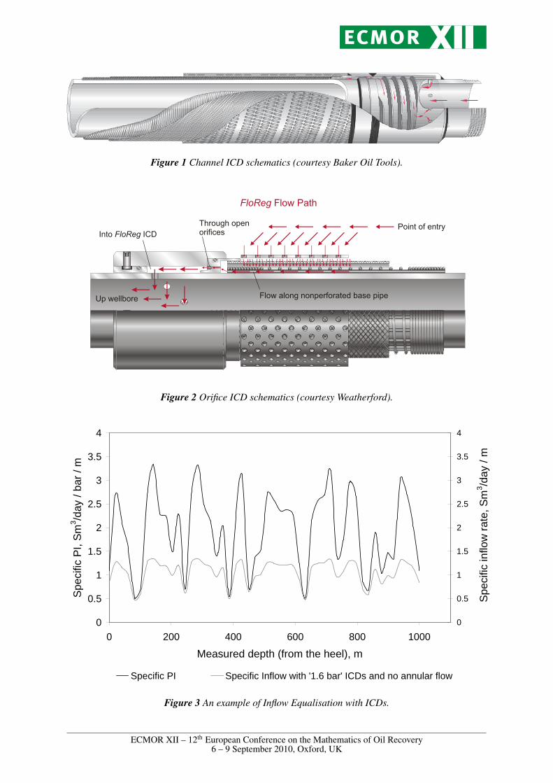
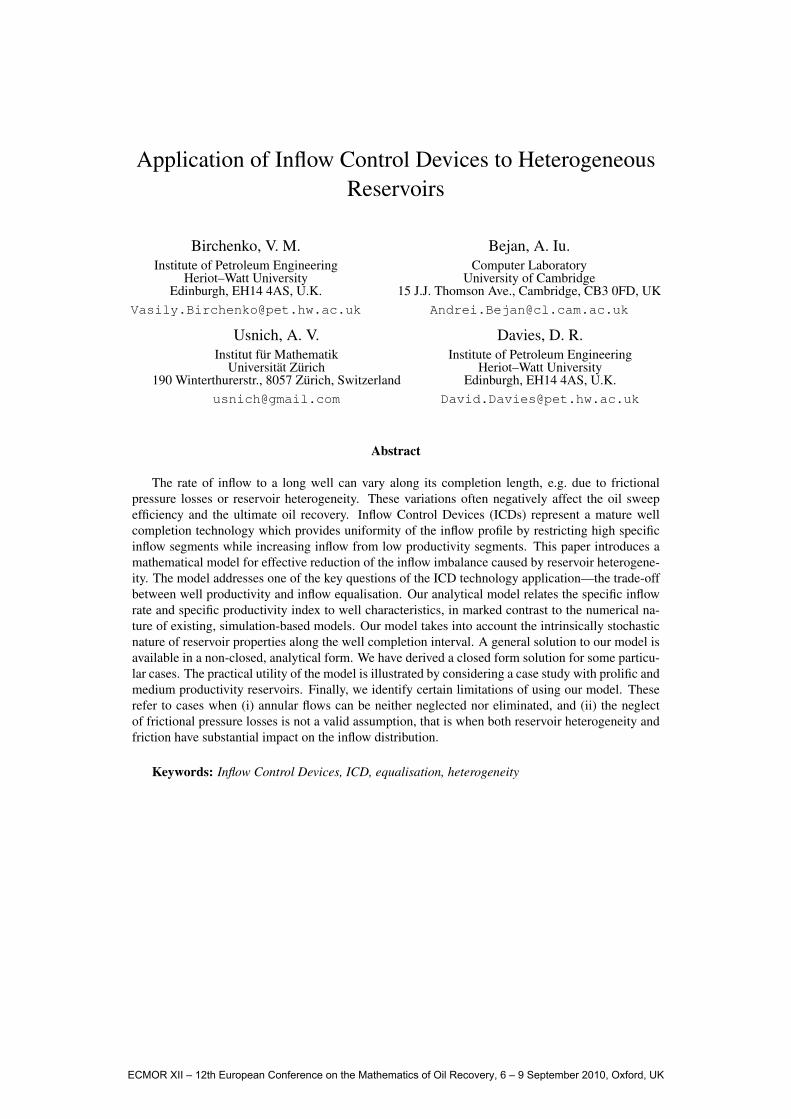
Figure 1 Channel ICD schematics (courtesy Baker Oil Tools).

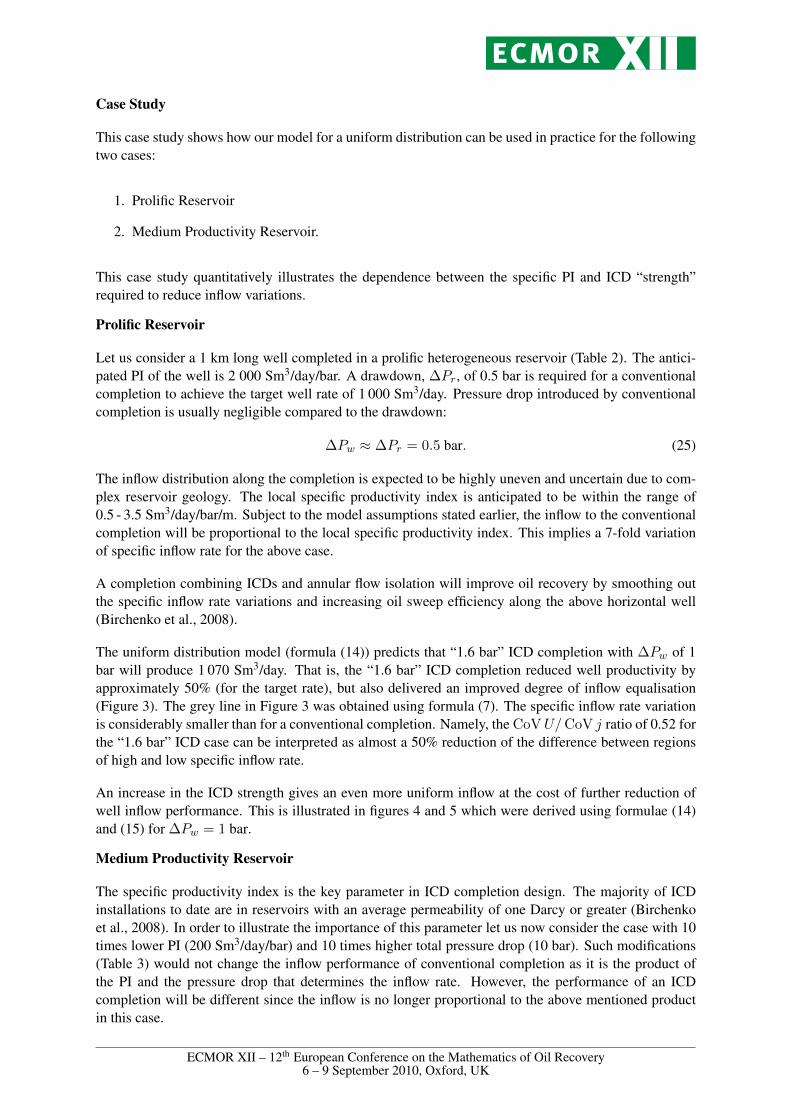
Figure 2 Orifice ICD schematics (courtesy Weatherford).

0

0.5

1

1.5

2

2.5

3

3.5

4

0 200 400 600 800 1000

Measured depth (from the heel), m

Spe

cific

PI,

Sm

3 /day

/ ba

r / m

0

0.5

1

1.5

2

2.5

3

3.5

4

Spe

cific

inflo

w ra

te, S

m3 /d

ay /

m

Specific PI Specific Inflow with '1.6 bar' ICDs and no annular flow

Figure 3 An example of Inflow Equalisation with ICDs.


0

0.2

0.4

0.6

0.8

1

1.2

0 0.001 0.002 0.003 0.004 0.005 0.006 0.007

Channel ICD strength, bar/(Rm3/day)2

CoV

ratio

0

500

1000

1500

2000

2500

Wel

l flo

w ra

te, S

m3 /d

ay

CoV ratio Well flow rate

Figure 4 Dependence of inflow equalisation and well productivity on ICD strength for channel ICDs ina prolific reservoir.

0

0.2

0.4

0.6

0.8

1

1.2

0 2 4 6 8 10 12 14 16

Effective nozzle diameter per 40 ft joint, mm

CoV

ratio

0

500

1000

1500

2000

2500

Wel

l flo

w ra

te, S

m3 /d

ay


Figure 5 Dependence of inflow equalisation and well productivity on ICD strength for nozzle/orificeICDs in a prolific reservoir.


0

0.2

0.4

0.6

0.8

1

1.2

0 0.001 0.002 0.003 0.004 0.005 0.006 0.007

Channel ICD strength, bar/(Rm3/day)2

CoV

ratio

0

500

1000

1500

2000

2500

Wel

l flo

w ra

te, S

m3 /d

ay


Figure 6 Dependence of inflow equalisation and well productivity on ICD strength for channel ICDs ina medium productivity reservoir.

0

0.2

0.4

0.6

0.8

1

1.2

0 2 4 6 8 10 12 14 16

Effective nozzle diameter per 40 ft joint, mm

CoV

ratio

0

500

1000

1500

2000

2500

Wel

l flo

w ra

te, S

m3 /d

ay


Figure 7 Dependence of inflow equalisation and well productivity on ICD strength for nozzle/orificeICDs in a medium productivity reservoir.


application of inﬂow control devices to heterogeneous ...aib29/icd_het_ecmor_xii.pdf ·...

Documents