APPLICATION OF BAYESIAN FILTERS TO HEAT CONDUCTION PROBLEMS

Helcio R. B. Orlande

Department of Mechanical Engineering, Politécnica/COPPE Federal University of Rio de Janeiro, UFRJ

Rio de Janeiro, RJ, Brazil helcio@mecanica.coppe.ufrj.br

George S. Dulikravich

Department of Mechanical and Materials Engineering Florida International University

Miami, Florida, U.S.A. dulikrav@fiu.edu

Marcelo J. Colaço

Department of Mechanical and Materials Engineering Military Institute of Engineering

Rio de Janeiro, RJ, Brazil colaco@asme.org

ABSTRACT

In this paper we present a general description of state estimation problems within the Bayesian framework. State estimation problems are addressed in which evolution and measurement stochastic models are used to predict the dynamic behavior of physical systems. Specifically, the application of two Bayesian filters to linear and non-linear unsteady heat conduction problems is demonstrated; a) the use of Kalman filter, and b) the use of Particle Filter with sampling importance resampling algorithm. Limitations of the filtering methodologies used in this work are presented involving different probability distributions for the errors in the models.

INTRODUCTION

State estimation problems, also designated as nonstationary inverse problems [1],

are of great interest in innumerable practical applications. In such kinds of problems, the

available measured data is used together with prior knowledge about the physical

phenomena and the measuring devices, in order to sequentially produce estimates of the

desired dynamic variables. This is accomplished in such a manner that the error is

minimized statistically [2]. For example, the position of an aircraft can be estimated

through the time-integration of its velocity components since departure. However, it may

also be measured with a GPS system and an altimeter. State estimation problems deal

with the combination of the model prediction (integration of the velocity components that

contain errors due to the velocity measurements) and the GPS and altimeter

measurements that are also uncertain, in order to obtain more accurate estimations of the

system variables (aircraft position).

State estimation problems are solved with the so-called Bayesian filters [1,2]. In

the Bayesian approach to statistics, an attempt is made to utilize all available information

in order to reduce the amount of uncertainty present in an inferential or decision-making

problem. As new information is obtained, it is combined with previous information to

form the basis for statistical procedures. The formal mechanism used to combine the new

information with the previously available information is known as Bayes’ theorem [1,3].

The most widely known Bayesian filter method is the Kalman filter [1,2,4-9].

However, the application of the Kalman filter is limited to linear models with additive

Gaussian noise. Extensions of the Kalman filter were developed in the past for less

restrictive cases, by using linearization techniques [1,3,6,7,8]. Similarly, Monte Carlo

methods have been developed in order to represent the posterior density in terms of

random samples and associated weights. Such Monte Carlo methods are usually denoted

as particle filters, among other designations found in the literature, and they do not

require the restrictive hypotheses of the Kalman filter. Hence, particle filters can be

applied to non-linear models with non-Gaussian errors [1,4,8-17].

In this paper we apply the Kalman filter and the particle filter to heat conduction

problems. These Bayesian filters are used to predict the temperature in a medium where

the heat conduction model and temperature measurements contain errors. Linear and non-

linear heat conduction problems are examined, as well as Gaussian and non-Gaussian

noise. Before focusing on the heat conduction applications of interest, the state estimation

problem is defined and the Kalman and particle filters are described.

STATE ESTIMATION PROBLEM

In order to define the state estimation problem, consider a model for the evolution

of the vector x in the form

(1.a)

where the subscript k = 1, 2, …, denotes an instant tk in a dynamic problem. The vector

is called the state vector and contains the variables. Their time evolution is of

interest to be tracked. This vector advances in accordance with the state evolution model

given by equation (1.a), where f is a non-linear function of the state variables and of the

state noise vector .

Consider also that measurements are available at tk, k = 1, 2, …. The

measurements are related to the state variables x through the non-linear function h in the

form

(1.b)

where is the measurement noise. Equation (1.b) is referred to as the observation

(measurement) model.

The state estimation problem aims at obtaining information about xk based on the

state evolution model (1.a) and on the measurements given by the

observation model (1.b) [1-17].

The evolution-observation model given by equations (1.a,b) are based on the

following assumptions [1,4]:

(i) The sequence for k = 1, 2, …, is a Markovian process, that is,

(2.a)

(ii) The sequence for k = 1, 2, …, is a Markovian process with respect to

the history of , that is,

(2.b)

(iii) The sequence depends on the past observations only through its own

history, that is,

(2.c)

where denotes the conditional probability of a when b is given.

In addition, for the evolution-observation model given by equations (1.a,b) it is

assumed that for the noise vectors and , as well as and , are mutually

independent and also mutually independent of the initial state . The vectors and

are also mutually independent for all i and j [1].

Different problems can be considered with the above evolution-observation

problem, namely [1]:

(i) The prediction problem, concerned with the determination of ;

(ii) The filtering problem, concerned with the determination of ;

(iii) The fixed-lag smoothing problem, concerned the determination of

, where is the fixed lag;

(iv) The whole-domain smoothing problem, concerned with the determination of

, where is the complete sequence of

measurements.

This paper deals only with the filtering problem. By assuming that

is available, the posterior probability density is then obtained

with Bayesian filters in two steps [1-17]: prediction and update, as illustrated in figure 1.

The Kalman filter and the particle filter used in this work are discussed below.

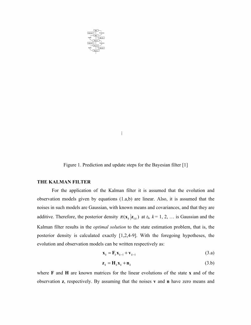
Figure 1. Prediction and update steps for the Bayesian filter [1]

THE KALMAN FILTER

For the application of the Kalman filter it is assumed that the evolution and

observation models given by equations (1.a,b) are linear. Also, it is assumed that the

noises in such models are Gaussian, with known means and covariances, and that they are

additive. Therefore, the posterior density at tk, k = 1, 2, … is Gaussian and the

Kalman filter results in the optimal solution to the state estimation problem, that is, the

posterior density is calculated exactly [1,2,4-9]. With the foregoing hypotheses, the

evolution and observation models can be written respectively as:

(3.a)

(3.b)

where F and H are known matrices for the linear evolutions of the state x and of the

observation z, respectively. By assuming that the noises v and n have zero means and

covariance matrices Q and R, respectively, the prediction and update steps of the Kalman

filter are given by [1,2,4-9]:

Prediction:

(4.a)

(4.b)

Update:

(5.a)

(5.b)

(5.c)

The matrix K is called Kalman’s gain matrix. Notice above that after predicting

the state variable x and its covariance matrix P with equations (4.a,b), a posteriori

estimates for such quantities are obtained in the update step with the utilization of the

measurements z.

For other cases for which the hypotheses of linear Gaussian evolution-observation

models are not valid, the use of the Kalman filter does not result in optimal solutions

because the posterior density is not analytic. The application of Monte Carlo techniques

then appears as the most general and robust approach to non-linear and/or non-Gaussian

distributions [1,4,8-17]. This is the case despite the availability of the so-called extended

Kalman filter, which involves a linearization of the problem. A Monte Carlo filter is

described below.

PARTICLE FILTER

One of the available Monte Carlo techniques for the state estimation problem is the

Particle Filter Method [1,4,8-17], also known as the bootstrap filter, condensation

algorithm, interacting particle approximations and survival of the fittest [8]. The key idea is

to represent the required posterior density function by a set of random samples (particles)

with associated weights, and to compute the estimates based on these samples and weights.

As the number of samples becomes very large, this Monte Carlo characterization becomes

an equivalent representation of the posterior probability function, and the solution

approaches the optimal Bayesian estimate.

We present below the so-called Sequential Importance Sampling (SIS) algorithm

for the particle filter, which includes a resampling step at each instant, as described in detail

in references [8,9]. The SIS algorithm makes use of an importance density, which is a

density proposed to represent another one that cannot be exactly computed, that is, the

sought posterior density in the present case. Then, samples are drawn from the importance

density instead of the actual density.

Let be the particles with associated weights and

be the set of all states up to tk, where N is the number of particles.

The weights are normalized so that . Then, the posterior density at tk can be

discretely approximated by:

(6.a)

where δ(.) is the Dirac delta function. By taking the hypothesis (2.a) into account, the

posterior density (6.a) can be written as:

(6.b)

A common problem with the SIS particle filter is the degeneracy phenomenon,

where after a few states all but one particle will have negligible weight [1,4,8-17]. This

degeneracy implies that a large computational effort is devoted to updating particles whose

contribution to the approximation of the posterior density function is almost zero. This

problem can be overcome by increasing the number of particles, or more efficiently by

appropriately selecting the importance density as the prior density . In addition,

the use of the resampling technique is recommended to avoid the degeneracy of the

particles.

Resampling involves a mapping of the random measure into a random

measure with uniform weights. It can be performed if the number of effective

particles with large weights falls below a certain threshold number. Alternatively,

resampling can also be applied indistinctively at every instant tk, as in the Sampling

Importance Resampling (SIR) algorithm described in [8,9]. Such algorithm can be

summarized in the following steps, as applied to the system evolution from tk-1 to tk [8,9]:

Step 1. For i=1,…, N draw new particles from the prior density and

then calculate the correspondent weights from the likelihood density

.

Step 2. Calculate the total weight and then normalize the particle

weights, that is, for i=1,…, N let .

Step 3. Resample the particles as follows:

Step 3.1. Construct the cumulative sum of weights (CSW) by computing

for i = 1,…, N, with .

Step 3.2. Let i = 1 and draw a starting point from the uniform distribution

.

Step 3.3. For j = 1, …, N

• Move along the CSW by making .

• While make i = i +1.

• Assign sample .

• Assign weight .

Although the resampling step reduces the effects of the degeneracy problem, it

may lead to a loss of diversity among the particles and the resultant sample will contain

many repeated points. This problem, known as sample impoverishment, can be severe in

the case of small process noise. In this situation, all particles collapse to a single particle

within few instants tk [1,8,9]. Another drawback of the particle filter is related to the large

computational cost due to the Monte Carlo method, which may limit its application to

complicated physical problems.

RESULTS AND DISCUSSIONS

In this session we apply the Bayesian filters described above to the estimation of

the transient temperature field in heat conducting media. Linear and non-linear heat

conduction problems are addressed, as well as different models for the noises. The

problems under study are described below and the results obtained with the Kalman and

particle filters are discussed.

Linear Heat Conduction Problem

Consider heat conduction in a semi-infinite one-dimensional medium, initially at

the uniform temperature T*. The temperature at boundary x = 0 is kept at T = 0 oC.

Physical properties are constant and there is no heat generation in the medium. The

formulation for this problem is given by:

in x > 0, for t > 0 (7.a)

at x=0, for t > 0 (7.b)

for t=0, in x > 0 (7.c)

The analytical solution for this problem is given by [18]:

(8)

The discretization of equation (7.a) by using explicit finite-differences results in:

(9)

where the superscript k denotes the time step, the subscript i denotes the finite-difference

node and

(10)

For the solution of problem (7.a-c) with finite-differences we have to impose a

boundary condition at some fictitious boundary at x=L. We assume L sufficiently large

for the time range of interest, so that the finite domain behaves as a semi-infinite

medium. Temperature at the boundary x=L was assumed to be T*.

The finite-difference solution for problem (7.a-c) can be written as:

(11)

where

(12.a-c)

In the equations above N is the number of internal nodes in the finite-difference

discretization. Matrix F is NxN and vector S is Nx1.

Equation (11) is in appropriate form for the application of the Kalman filter (see

equation 3.a). In the present example it is assumed that state and measured variables are

the transient temperatures inside the medium at the equidistant finite difference nodes.

Therefore, matrix H for the observation model (see equation 3.b) is the identity matrix.

The medium is considered to be concrete, with thermal diffusivity α = 4.9x10-7

m2/s. The standard deviation for the measurement errors is considered constant and equal

to 2 oC. The effects of the standard deviation of the errors in the state model are examined

below. Figures 2.a and 2.b present the exact temperatures and the measured temperatures

in the region, respectively. The final time is taken as 250 seconds and measurements are

supposed available in the region every 1 second. The fictitious thickness of the medium is

considered to be L = 0.1 m and the region is discretized with N = 50 internal nodes.

Figure 2.a – Exact temperatures

Figure 2.b – Measured temperatures containing Gaussian errors with standard deviation

of 2 oC

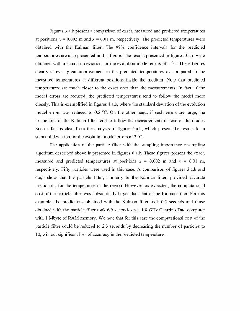
Figures 3.a,b present a comparison of exact, measured and predicted temperatures

at positions x = 0.002 m and x = 0.01 m, respectively. The predicted temperatures were

obtained with the Kalman filter. The 99% confidence intervals for the predicted

temperatures are also presented in this figure. The results presented in figures 3.a-d were

obtained with a standard deviation for the evolution model errors of 1 oC. These figures

clearly show a great improvement in the predicted temperatures as compared to the

measured temperatures at different positions inside the medium. Note that predicted

temperatures are much closer to the exact ones than the measurements. In fact, if the

model errors are reduced, the predicted temperatures tend to follow the model more

closely. This is exemplified in figures 4.a,b, where the standard deviation of the evolution

model errors was reduced to 0.5 oC. On the other hand, if such errors are large, the

predictions of the Kalman filter tend to follow the measurements instead of the model.

Such a fact is clear from the analysis of figures 5.a,b, which present the results for a

standard deviation for the evolution model errors of 2 oC.

The application of the particle filter with the sampling importance resampling

algorithm described above is presented in figures 6.a,b. These figures present the exact,

measured and predicted temperatures at positions x = 0.002 m and x = 0.01 m,

respectively. Fifty particles were used in this case. A comparison of figures 3.a,b and

6.a,b show that the particle filter, similarly to the Kalman filter, provided accurate

predictions for the temperature in the region. However, as expected, the computational

cost of the particle filter was substantially larger than that of the Kalman filter. For this

example, the predictions obtained with the Kalman filter took 0.5 seconds and those

obtained with the particle filter took 6.9 seconds on a 1.8 GHz Centrino Duo computer

with 1 Mbyte of RAM memory. We note that for this case the computational cost of the

particle filter could be reduced to 2.3 seconds by decreasing the number of particles to

10, without significant loss of accuracy in the predicted temperatures.

Figure 3.a – Temperature at x = 0.002 m – standard deviation for the evolution model

errors of 1 oC – Kalman filter

Figure 3.b – Temperature at x = 0.01 m – standard deviation for the evolution model

errors of 1 oC – Kalman filter

Figure 4.a. Temperature at x = 0.002 m – standard deviation for the evolution model

errors of 0.5 oC – Kalman filter

Figure 4.b. Temperature at x = 0.01 m – standard deviation for the evolution model errors

of 0.5 oC – Kalman filter

Figure 5.a. Temperature at x = 0.002 m – standard deviation for the evolution model errors of

5 oC – Kalman filter

Figure 5.b. Temperature at x = 0.01 m – standard deviation for the evolution model errors

of 5 oC – Kalman filter

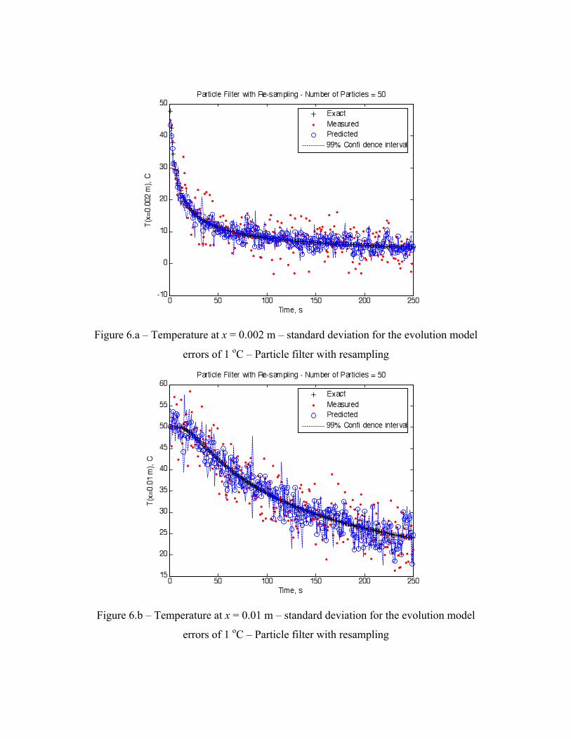
Figure 6.a – Temperature at x = 0.002 m – standard deviation for the evolution model

errors of 1 oC – Particle filter with resampling

Figure 6.b – Temperature at x = 0.01 m – standard deviation for the evolution model

errors of 1 oC – Particle filter with resampling

Figures 7.a,b present results similar to those of figures 6.a,b, but without using the

resampling technique. These figures show that the predictions obtained without

resampling were quite uncertain, that is, with large confidence intervals. On the other

hand, sample impoverishment can be observed when resampling was used, which is

characterized by the very narrow confidence intervals for the predicted temperatures

shown in figures 6.a,b.

We now examine a case involving uniformly distributed errors in the evolution

model, instead of Gaussian errors. For such case, the application of the Kalman filter did

not result in optimal solutions. Consequently, only the particle filter was considered for

the prediction of the temperatures in the region. The results obtained with errors in the

evolution model uniformly distributed in the interval [-1,1] oC are presented in figures

8.a,b for x = 0.002 m and x = 0.01 m, respectively. These figures show that the particle

filter was not affected by the distribution of the errors and results similar to those

obtained for the Gaussian distribution (see figures 6.a,b) were obtained.

Figure 7.a – Temperature at x = 0.002 m – standard deviation for the evolution model

errors of 1 oC – Particle filter without resampling

Figure 7.b – Temperature at x = 0.01 m – standard deviation for the evolution model

errors of 1 oC – Particle filter without resampling

Figure 8.a – Temperature at x = 0.002 m - evolution model errors having uniform

distribution in [-1,1] oC – Particle filter

Figure 8.b – Temperature at x = 0.01 m - evolution model errors having uniform

distribution in [-1,1] oC – Particle filter

Nonlinear Heat Conduction Problem

Consider heat conduction in a one-dimensional medium with thickness L, initially

at the uniform temperature T*. The boundary at x = 0 is kept insulated and a constant heat

flux q* is imposed at x = L. Thermophysical properties are temperature dependent and

there is no heat generation in the medium. The formulation for this problem is given by:

in 0 < x < L, for t > 0 (13.a)

at x=0, for t > 0 (13.b)

at x=L, for t > 0 (13.c)

for t=0, in x > 0 (13.d)

We examine here a physical problem similar to those examined in references

[19,20] involving the heating of a graphite sample with an oxy-acetylene torch. The

temperature dependence of the thermal conductivity, k(T), and volumetric heat capacity,

C(T), of the graphite, measured for different temperatures, were curve-fitted (see figure

9) with exponentials of the form:

(14.a)

(14.b) with the adjusted parameters A1, A2, A3, B1, B2 and B3 given in table 1.

Table 1. Parameters of the curve-fitted thermophysical properties Parameter Mean

A1 (Jm-3 ºC-1) 5,681,006 A2 (Jm-3 ºC-1) 4,813,057

A3 (ºC) 547.00 B1 (Wm-1 ºC-1) 24.52 B2 (Wm-1 ºC-1) 183.05

B3 (ºC) 277.00

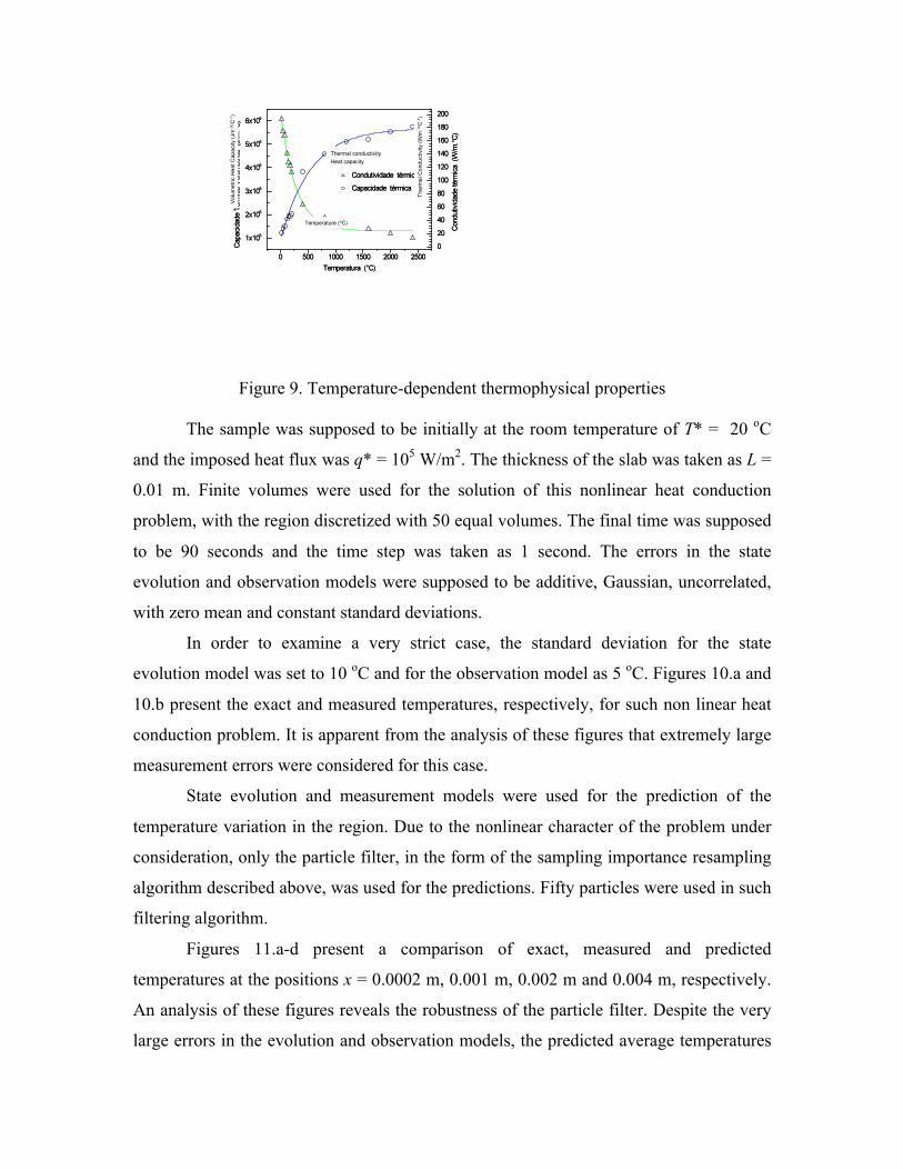
Figure 9. Temperature-dependent thermophysical properties

The sample was supposed to be initially at the room temperature of T* = 20 oC

and the imposed heat flux was q* = 105 W/m2. The thickness of the slab was taken as L =

0.01 m. Finite volumes were used for the solution of this nonlinear heat conduction

problem, with the region discretized with 50 equal volumes. The final time was supposed

to be 90 seconds and the time step was taken as 1 second. The errors in the state

evolution and observation models were supposed to be additive, Gaussian, uncorrelated,

with zero mean and constant standard deviations.

In order to examine a very strict case, the standard deviation for the state

evolution model was set to 10 oC and for the observation model as 5 oC. Figures 10.a and

10.b present the exact and measured temperatures, respectively, for such non linear heat

conduction problem. It is apparent from the analysis of these figures that extremely large

measurement errors were considered for this case.

State evolution and measurement models were used for the prediction of the

temperature variation in the region. Due to the nonlinear character of the problem under

consideration, only the particle filter, in the form of the sampling importance resampling

algorithm described above, was used for the predictions. Fifty particles were used in such

filtering algorithm.

Figures 11.a-d present a comparison of exact, measured and predicted

temperatures at the positions x = 0.0002 m, 0.001 m, 0.002 m and 0.004 m, respectively.

An analysis of these figures reveals the robustness of the particle filter. Despite the very

large errors in the evolution and observation models, the predicted average temperatures

are in excellent agreement with the exact values. Furthermore, the 99% confidence

intervals for the predicted temperatures are significantly smaller than the dispersion of the

measurements. Differently from the case analyzed above involving linear heat

conduction, sample impoverishment is not observed in figures 11.a-d. This is probably

due to the large noise in the state model used for the nonlinear case. The computational

time for this case was 61.3 seconds.

Figure 10.a – Exact temperatures

Figure 10.b – Measured temperatures containing Gaussian errors with standard deviation

Figure 11.a – Temperature at x = 0.0002 m for the nonlinear heat conduction problem –

Particle filter

Figure 11.b – Temperature at x = 0.001 m for the nonlinear heat conduction problem –

Particle filter

Figure 11.c – Temperature at x = 0.002 m for the nonlinear heat conduction problem –

Particle filter

Figure 11.d – Temperature at x = 0.004 m for the nonlinear heat conduction problem –

Particle filter

REFERENCES

1. Kaipio, J. and Somersalo, E., 2004, Statistical and Computational Inverse Problems, Applied Mathematical Sciences 160, Springer-Verlag.

2. Maybeck, P., 1979, Stochastic models, estimation and control, Academic Press, New York.

3. Winkler, R., 2003, An Introduction to Bayesian Inference and Decision, Probabilistic Publishing, Gainsville.

4. Kaipio, J., Duncan S.,Seppanen, A., Somersalo, E., Voutilainen, A., 2003, State Estimation, Chapter in

5. Kalman, R., 1960, A New Approach to Linear Filtering and Prediction Problems, ASME J. Basic Engineering, vol. 82, pp. 35-45.

6. Sorenson, H., 1970, Least-squares estimation: from Gauss to Kalman, IEEE Spectrum, vol. 7, pp. 63-68.

7. Welch, G. and Bishop, G., 2006, An Introduction to the Kalman Filter, UNC-Chapel Hill, TR 95-041.

8. Arulampalam, S., Maskell, S., Gordon, N., Clapp, T., 2001, A Tutorial on Particle Filters for on-line Non-linear/Non-Gaussian Bayesian Tracking, IEEE Trans. Signal Processing, vol. 50, pp. 174-188.

9. Ristic, B., Arulampalam, S., Gordon, N., 2004, Beyond the Kalman Filter, Artech House, Boston.

10. Doucet, A., Godsill, S., Andrieu, C., 2000, On sequential Monte Carlo sampling methods for Bayesian filtering, Statistics and Computing, vol. 10, pp. 197-208.

11. Liu, J and Chen, R., 1998, Sequential Monte Carlo methods for dynamical systems, J. American Statistical Association, vol. 93, pp. 1032-1044.

12. Andrieu, C., Doucet, A., Robert, C., 2004, Computational advances for and from Bayesian analysis, Statistical Science, vol. 19, pp. 118-127.

13. Johansen, A. Doucet, A., 2008, A note on auxiliary particle filters, Statistics and Probability Letters, to appear.

14. Carpenter, J., Clifford, P., Fearnhead, P, 1999, An improved particle filter for non-linear problems, IEEE Proc. Part F: Radar and Sonar Navigation, vol. 146, pp. 2-7.

15. Del Moral, P., Doucet, A., Jasra, A., 2007, Sequential Monte Carlo for Bayesian Computation, Bayesian Statistics, vol. 8, pp. 1-34.

16. Del Moral, P., Doucet, A., Jasra, A., 2006, Sequential Monte Carlo samplers, J. R. Statistical Society, vol. 68, pp. 411-436.

17. Andrieu, C., Doucet, Sumeetpal, S., Tadic, V., 2004, Particle methods for charge detection, system identification and control, Proceedings of IEEE, vol. 92, pp. 423-438.

18. Ozisik, M., 1993, Heat Conduction, Wiley, New York. 19. Mota, C. A. A., Mikhailov, M. D., Orlande, H. R. B. and Cotta, R. M., 2004,

Identification of Heat Flux Imposed by an Oxyacetylene Torch, AIAA paper ????, 10th AIAA/ISSMO Multidisciplinary Analysis and Optimization Conference, Albany, New York, August 29 – September 2.

20. Mota, C. A. A., Orlande, H. R. B., Wellele, O., Kolehmainen, V. and Kaipio, J., 2007, Inverse Problem of Simultaneous Identification of Thermophysical

Properties and Boundary Heat Flux, 19th COBEM -International Congress of Mechanical Engineering, November 5-9, 2007, Brasilia, Brazil.