application of assignment problem with side constraints · es this problem from many other...
TRANSCRIPT

VU University Amsterdam Faculty of Sciences
Application of assignment problem with side constraints
Workload balancing between warehouse zones for product families
Master project Business Analytics
Bas de Jong

This page is intentionally left blank

VU University Amsterdam Faculty of Sciences
Application of assignment problem with side constraints
Workload balancing between warehouse zones for product families
Master project Business Analytics
Bas de Jong
June 2015
Under supervision of: Dr. Kristiaan Glorie Dr. Sandjai Bhulai
VU University Amsterdam Valeant Pharmaceuticals Faculty of Sciences European Logistics Center De Boelelaan 1081 Koolhovenlaan 110 1081 HV Amsterdam 1119 NH Schiphol-Rijk

This page is intentionally left blank

Dedicated to the memory of Peter

This page is intentionally left blank

Page i
Preface This thesis is the culmination of 4 years of hard work during which I combined my Business Analytics study with my job at Bausch + Lomb and, since the mid 2013 acquisition, Valeant Pharmaceuticals. Already working for more than 5 years since my graduation, I became dissatisfied with the level of depth that was offered in training for professionals. I wanted to expand my personal toolkit to tackle optimization problems that the organization was facing and to develop good decision support tools. The VU University was offering a dual Master study that appeared to fit my needs. The thought of going back to school excited me rather than scared me. Looking back I sometimes still wonder how I have managed to combine both work and study, while maintaining somewhat of a social life. It required not only much dedication and flexibility from me, but the flexibility was also requested from my colleagues, friends and girlfriend. Without their support I wouldn’t have been able to complete this study. Mainly I want to thank Sandra Geelink for supporting me from the beginning and paving the way within the organization to get this crazy idea accepted. A lot of thanks also goes out to my colleagues Niels and Herman for covering me during my study hours. My friends and family might not have seen me as much in the past 4 years as I would like to, but with lots of free time coming up with the conclusion of this thesis I will make it up to them. But most thanks goes out to my girlfriend Tryntje for the patience and support not only during the past 4 years, but the 8 years that we are together. This thesis wouldn’t have been possible without the help of some other people. I would like to thank Niels again, now for being my company mentor during the thesis phase and showing a lot of confidence in me. From the VU University I appreciate the feedback and talks with my mentors Kristiaan Glorie and Sandjai Bhulai. Their ideas in a field that was relatively new to me helped to get and stay on track during a demanding and sometimes difficult year. Thank you for your guidance and making this possible. Amsterdam, June 2015

Page ii
Page iii
Summary Workload balancing between zones helps to reduce the risk for bottlenecks on the conveyor system for Valeant Pharmaceuticals’ European Logistics Centre at Schiphol-Rijk. They want to know whether a faster and more efficient method to update the product assignment can be devised. 2,659 products need to be assigned to 6 stations, each consisting of 6 zones. Each zone is split in a high pick capacity flowrack and a lower capacity backrack. It is the objective of this study to reduce the workload for the Business Analyst by generating an acceptable product assignment. The principal question of this study is: In what ways is it possible to generate a feasible product assignment within 8 hours that is within 5% from the optimal solution, while satisfying the constraints? The problem in NP-hard and most resembles a categorized bottleneck assignment problem with loose capacity constraints. On top of this, three unique side constraints are added: products from the same product family need to be assigned to the same station (Station constraint), products need to be assigned in a specific order to the zones of a station (Power constraint) and the number of product moves that can be executed is limited. For the individual constraints almost no references in literature have been found and none for the combination of the three. Algorithms using heuristics such as variable and Lagrange relaxation, tabu search and branch and bound have been successfully used on assignment problems and could provide a good basis for this problem as well. The problem is analysed with AIMMS modelling software and the CPLEX algorithm. The algorithms are first tested on smaller scaled version of the problem and the performance is initially assessed based on the root node processing time and the LP-root incumbent gap. In all cases at least two runs of each problem instances are executed. The focus in this research is mainly on the effect of the three side constraints on the solvability of the problem, relaxation of variables and the effect of big-M constant on the performance of the algorithm. The problem, formulated as an ILP problem, cannot be solved to within 5% from optimality in 8 hours. In part because of the complexity the Power constraint adds to the problem. This constraint is dropped in conjunction with Valeant. Even the ILP problem without Power constraint does not generate an acceptable solution. Relaxation of variables was studied next. The problem is transformed to a LP problem by relaxing all variables. This leads to undesirable effects as the Station constraint is not enforced properly. The application of two-step fractional rounding solves this problem but leads to a violation of the move constraint. By relaxing all variables except for xip, which controls the assignment of the product families to stations, the problem becomes a MILP problem. Good results within 5% of optimality are found within two hours of model run time. To solve issues caused by fractional rounding it is recommended to set the number of allowed moves to 5 less than the desired maximum of moves. The results obtained with the MILP problem are better than those of the LP problem measured by mean absolute deviation between zones. Setting a sharp bound for big-M will help to obtain better or faster results for this problem compared to large valued big-M and the indicator constraint method recommended by AIMMS. From the results can also be concluded that the optimal result can already be achieved by moving only a third of the products. For the validation set the mean absolute deviation between the zones is already reduced by more than 90% by executing 150 moves, with a maximum reduction possible of 98%. Using MILP software and the partially relaxed model with zone capacity constraints, maximum moves constraint and Station constraint a feasible product assignment can be generated within 8 hours and 5% from optimality.
Page iv
Contents Preface ...................................................................................................................................................... i
Summary ................................................................................................................................................. iii
1. Introduction ......................................................................................................................................... 1
1.1 Problem background ..................................................................................................................... 1
1.2 Problem characteristics ................................................................................................................. 3
1.3 Problem statement ........................................................................................................................ 3
1.4 Outline ........................................................................................................................................... 4
2. Problem formulation ........................................................................................................................... 5
3. Theoretical background ....................................................................................................................... 7
3.1 Product assignments in warehouses ............................................................................................. 7
3.2 The assignment problem ............................................................................................................... 9
3.2.1 Various objective functions .................................................................................................... 9
3.2.2 Resource constrained assignment problem ......................................................................... 10
3.2.3 Semi-assignment problem .................................................................................................... 11
3.2.4 Categorized bottleneck assignment problem ...................................................................... 12
3.3 Literature conclusions ................................................................................................................. 13
4. Methodology ..................................................................................................................................... 15
4.1 Problems ...................................................................................................................................... 15
4.2 Tools and settings ........................................................................................................................ 16
4.3 Data collection ............................................................................................................................. 17
4.3.1 Alternative assignment ......................................................................................................... 18
4.3.2 Scaled model ........................................................................................................................ 18
4.4 Outline of research ...................................................................................................................... 20
4.4.1 Root node analysis ............................................................................................................... 20
4.4.2 Selection of scaled model ..................................................................................................... 20
4.4.3 Verification and validation ................................................................................................... 21
5. Results ............................................................................................................................................... 23
5.1 Objective function ....................................................................................................................... 23
5.2 Effect of side constraints ............................................................................................................. 23
5.2.1 Station and power constraints ............................................................................................. 24
5.2.2 Maximum moves allowed .................................................................................................... 25
5.3 Relaxation of variables ................................................................................................................ 27
5.3.1 LP problem............................................................................................................................ 27
5.3.2 Partially relaxed variables .................................................................................................... 28
5.4 The effect of big-M constant ....................................................................................................... 30
5.5 Complete model .......................................................................................................................... 32
6. Conclusions and recommendations .................................................................................................. 37

Page v
Appendix 1: Breakdown of locations on Mezzanine ............................................................................. 41
Appendix 2: Scaled model product family classification ....................................................................... 42
Appendix 3: AIMMS program code ....................................................................................................... 44
Bibliography ........................................................................................................................................... 49

Page vi

Page 1
1. Introduction It is not uncommon for warehouses nowadays to store more than 100,000 different products. With so many products spread over a warehouse, it is not hard to imagine that a lot of efficiency with respect to walking distances or order throughput time can be gained by having the right product at the right location. This thesis focuses on the assignment of products to locations of a section of a warehouse, in this case the European Logistics Center of Valeant Pharmaceuticals. What distinguish-es this problem from many other assignment problems is the applications of a unique set of side constraints. First the problem background is discussed in Section 1.1, followed by the outline of the side constraints in Section 1.2. This results in a problem formulation with research questions in Section 1.3, followed by the outline of this thesis in Section 1.4.
1.1 Problem background Valeant Pharmaceuticals International (Valeant) is a multinational specialty pharmaceutical company that develops, manufactures and markets a broad range of pharmaceutical products primarily in the areas of dermatology, eye health, neurology and branded generics (Valeant 2015). With reported revenues of US $5.76 billion, it has offices and plants on all continents. The shares of the Canadian company are traded on the Toronto and New York stock exchange. In 2013 Valeant acquired Bausch + Lomb (B+L), a leading brand in ophthalmology. Founded more than 160 years ago in Rochester, New York, B+L has developed some industry changing products like Ray Ban sunglasses, the soft contact lens and Stellaris/PC. The European Logistics Center (ELC) at Schiphol-Rijk is Valeant’s largest distribution centre for ophthalmology products in Europe. The majority of the order volume concerns Bausch + Lomb products, with an increasing share of other Valeant brands. The fastest moving lens products are picked at the Pick-to-Light (PTL) area of the Mezzanine department. The area, which handles around 40% of the 34,000 daily picks, is a zone picking system consisting of 6 stations with pick-to-light functionality. With pick-to-light, the location and the quantity that needs to be picked is indicated on a display at or close to the picking location. This system reduces human pick errors with 95% according to research performed by Tolliver (Tolliver 1989). Each station, consisting of six zones, has buffering capacity before the first zone and exit and entry points to the main conveyor. All zones consist of flowracks and backracks. Flowracks are shelves designed for very fast-moving products up to 0.025 m3 and are automatically replenished by an automatic storage and retrieval system (AS/RS) from the back of the racking. Backracks are static racks for similar but slower moving products which are replenished manually. Figure 1 is a schematic drawing of two stations in the area. Orders, consisting of one or more orderlines, received before the cut-off time need to be processed the same working day. Orders received after cut-off, which varies between 13:00 and 16:00 and is country-specific, are processed the next working day. Orders that are finished not later than one hour after cut-off count towards the ELC pick performance metric, called ‘pick-pack performance’. This metric measures the percentage of orderlines shipped in time. The past three years the ELC has shipped 99.4% of the orderlines in time, while the target is set at 99%.

Page 2
Figure 1: schematic drawing of the Pick-to-Light area at the Mezzanine department Because orders are received throughout the day and the content of the orders is not known in advance, the workload per station and per zone varies on a daily or even hourly basis. To deal with this variance in demand, the basic operating principle at the ELC for the PTL area is to assign a single operator to each station and to have 2-3 more operators available to assist at stations that have a workload at that moment. Based on this, there can be 1-3 operators working in a single station at any moment of time. As each station is divided into 6 zones, each operator is responsible for 2 – 6 zones. ELC Operations management wants to spread out the workload evenly to reduce the risk for bottlenecks in the system as much as possible. Bottlenecks limit the capacity of the system and therefore can endanger the overall performance of the ELC, especially the pick-pack performance. This principle is supported by research of Jane (Jane 2000) and Yu and De Koster (Yu and De Koster 2008) that shows workload balancing reduces the order throughput time for a similar type pick system. The distribution of workload can be controlled by the assignment of products to pick locations in the stations of the PTL-area. Until recently, the product assignment in the PTL area was revised only once a year. Due to the introduction and discontinuation of various product families the frequency needs to be increased. Even though the workload distribution over the zones is reported and discussed on a monthly basis, a revision of the assignment is made only once a year by the Business Analyst because the process is labour intensive: a new assignment is created by hand in an Excel-document and it takes a couple of days to produce an acceptable, but non-optimal solution. A computer can explore solutions much faster and, using a smart algorithm, can produce the optimal solution or a near-optimal solution much faster. Therefore Valeant desires to reduce the time it takes to create a new assignment to 8 working hours, plus a maximum of 8 hours computer run time on desktop or laptop with 4 GB RAM. It also requires a considerable number of hours for the operators to execute all product moves. Often 25% or more of all products are moved to a new location to improve the workload balance. Valeant has a desire to spread the workload for these item moves. Rather than doing a large update and moving many products once a year, they would like to do more frequent updates while moving fewer items per update. To summarize, a faster and more automated approach will allow ELC operations management:
• to improve spreading of the workload by finding a solution closer to or at the optimum; • to execute small updates of the item location assignment more frequently, to stay close to
the optimal workload distribution; • to reduce the time that the Business Analyst spends on item placement.

Page 3
1.2 Problem characteristics As described earlier in this chapter, the PTL area consists of 6 stations with 6 zones each. Each zone has up to 18 flowrack locations and between 80 and 120 backrack locations. Products cannot be assigned to all backrack locations, as some locations in the backracks need to be reserved as so-called dynamic locations. Earlier analysis has shown that between 35% and 20% of the backrack locations per zone need to be reserved as dynamic locations. These dynamic locations are reserved for replenishment of products that do not have the same production lot-number as products already stored in the backracks, because the locations can only contain one lot-number. Since it concerns temporary assignments, the dynamic locations are not considered in the product assignment problem. The availability of locations in a zone or rack is a constraint for the problem. The products stored in the PTL-area are fast moving contact lens products, each belonging to a product family. The most popular product families consist of 30 – 130 individual products, each with a different dioptre, eye ball radius and/or cylinder. Three additional side constraints complicate the product assignment and two of them are related to this product family property. The first is that all products belonging to the same product family need to be assigned to the same station, from here on called the family-to-station constraint. This is done to minimize the number of stops an order has to make and thus to reduce the order processing time. To discuss the relation between order processing time and the number of stops is beyond the scope of this study, but this is recommended by the supplier of the warehouse management system (WMS). The second constraint is called power sequence. This comes from a system functionality called Power Sequence Picking which is provided by the supplier of the WMS for the customer’s convenience. Customer orders are picked in order of ascending dioptre (power) when products are assigned in order to the zones. This functionality is only activated with large orders, but requires that the products are stored in ascending order. Although the number or orders picked in power sequence is less than 10%, it is a service that was marketed to customers and is still offered. The third constraint, previously discussed in Section 1.1, is to limit the number of moves that can be executed.
1.3 Problem statement The objective of Valeant is to reduce the risk for bottlenecks on the conveyor system on the Mezzanine. The experience from Valeant is supported by research that distributing the workload evenly over the zones in the PTL-area contributes to this objective. To achieve or maintain an even balance, the assignment of products needs to be revised on a regular basis. Valeant wants to know whether a faster and more efficient method than the current can be devised to assist them in meeting their objective. It is the objective of this study to reduce the workload for the Business Analyst in generating an acceptable product assignment. Valeant considers the assignment acceptable if the zone workload deviation is within 5% of the optimum. The workload for the Business Analyst will decrease significantly if a new assignment can be generated within 4 working hours, plus a maximum computer run time of 8 hours on a desktop or laptop with 4 GB RAM. The principal question of this study is: In what ways is it possible to generate a feasible product assignment within 8 hours that is within 5% from the optimal solution, while satisfying the constraints? The answer to the principal question is found by answering the following derivative questions: 1. Can the described assignment problem with side constraints be solved to optimality for 2,659
products within 8 hours? 2. Which algorithms can be expected to be suitable for generating a (near) optimal assignment
given the time and memory constraint?

Page 4
3. How do (relaxed) side constraints influence the problem solvability and the solution feasibility? 4. How do (relaxed) variables influence the problem solvability and the solution feasibility? 5. How does the big M constant influence the solvability of the problem?
These questions will be answered in the next chapters. Implementation of the solution into a working program for Valeant is not part of the scope in this thesis. Recommendations for a successful implementation will be made in chapter 6.
1.4 Outline The remainder of this thesis is structured as follows: Chapter 2 provides a background for the problem based on scientific literature and provides a framework for the analysis to be conducted. In Chapter 3 the model is presented that will form the basis for the analysis. The methodology of the analysis is discussed in Chapter 4. Chapter 5 presents the results of the analysis, answering the research questions. The last chapter contains the conclusions and recommendations.

Page 5
2. Problem formulation The problem described in Chapter 1 can be written as an integer linear programming problem (ILP) where all decision variables take on binary values. Decision variables xijkpq = {0,1} where xijkpq = 1 when product pq is assigned to area ijk, else 0 xip = {0,1} where xip = 1 when family p is assigned to station i, else 0. mijkpq = {0,1} where mijkpq = 1 when product pq is moved from area ijk to another, else 0. With i = {1,…,I} the number of PTL stations, j = {1,…,J}, the number of zones in PTL station i, k = {1,2} the type of racking in zone j, either flowrack (1) of backrack (2). Regarding products, p = {1,..,P} is the identifier of the product family to be assigned and q = {1,…,Qp} is the sequence number of the item of family p. Objective function The objective is to minimize the difference between the zone with the highest workload and the lowest:
min max𝑖,𝑗�∑ ∑ ∑ 𝐷𝑝𝑞𝑥𝑖𝑗𝑘𝑝𝑞𝐿𝑘𝑞𝑝𝑘 � − min𝑖𝑗�∑ ∑ ∑ 𝐷𝑝𝑞𝑥𝑖𝑗𝑘𝑝𝑞𝐿𝑘𝑞𝑝𝑘 � Where Dpq are the cost (picks) associated with product pq and Lk the weight of assigning a products to rack k. Lk = 1 for k = 1 and Lk = 1.5 for k = 2. Constraints The two constraints below are standard constraints belonging to a semi-assignment problem.
��𝑥𝑖𝑗𝑘𝑝𝑞𝑞𝑝
≤ 𝑏𝑖𝑗𝑘 ∀ 𝑖, 𝑗,𝑘
���𝑥𝑖𝑗𝑘𝑝𝑞𝑘𝑗𝑖
= 1 ∀ 𝑝, 𝑞
Where bijk represents the number of locations available in area ijk Next to these basic constraints, several side constraints are introduced that are derived from the product family properties and the desire to limit the number of moves. Move constraints
�����𝑚𝑖𝑗𝑘𝑝𝑞 ≤ 𝑊𝑞𝑝𝑘𝑗𝑖
𝑥𝑖𝑗𝑘𝑝𝑞∗ − 𝑥𝑖𝑗𝑘𝑝𝑞 ≤ 𝑚𝑖𝑗𝑘𝑝𝑞 ∀ 𝑖, 𝑗,𝑘,𝑝, 𝑞 𝑚𝑖𝑗𝑘𝑝𝑞 ≥ 0
W represents the maximum number of products that are allowed to be moved from one location to another. This is a parameter that is set in advance. Parameter x*ijkpq is a binary matrix representing the current assignment of products.
Page 6
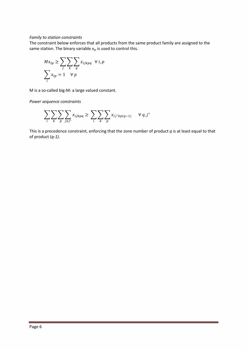
Family to station constraints The constraint below enforces that all products from the same product family are assigned to the same station. The binary variable xip is used to control this.
𝑀𝑥𝑖𝑝 ≥���𝑥𝑖𝑗𝑘𝑝𝑞𝑞𝑘𝑗
∀ 𝑖,𝑝
�𝑥𝑖𝑝𝑖
= 1 ∀ 𝑝
M is a so-called big-M: a large valued constant. Power sequence constraints
����𝑥𝑖𝑗𝑘𝑝𝑞𝑗≥𝑗∗𝑝𝑘𝑖
≥ ���𝑥𝑖𝑗∗𝑘𝑝(𝑞−1)𝑝𝑘𝑖
∀ 𝑞, 𝑗∗
This is a precedence constraint, enforcing that the zone number of product q is at least equal to that of product (q-1).

Page 7
3. Theoretical background In the previous chapter the basis for and the objective for this study were introduced. The next step is to check with existing scientific literature whether an existing algorithm can be used to meet the objective or that a new algorithm needs to be developed. In this chapter the literature concerning product assignments in warehouses is reviewed first, followed by a review of literature from a theoretical perspective.
3.1 Product assignments in warehouses During the last 25 years automation of warehouse operations has taken a flight. The introduction and further development of systems such as Automated Storage / Retrieval System (AS/RS), shuttle systems, pick-to-light (PTL), radio-frequency identification (RFID) and Automated Guided Vehicle Systems (AGVS) were introduced to help, amongst others, increase the output per order picker and decrease the order picking time. Because of this automation, the number of parts-to-picker systems is growing. However, based on De Koster’s experience the majority of the systems are still picker-to-parts, where pickers move within aisles to retrieve the required products. He (De Koster, Le-Duc et al. 2007) states that over 80% of all order-picking systems in Western Europe concern low-level picker-to-part systems. In these systems the order picker picks goods from a static storage rack without the use of reach trucks or cranes. Order picking cost, due to the labor intensive nature of the process, can contribute to 55% of the warehouse operating cost (Tompkins, White et al. 2003). Within the low-level picker-to-parts system, multiple variations exist. They can be classified based on the following choices, adapted from (De Koster 2004):
• Pick by article vs. pick by order. In the former case, the order picked multiple orders at the same time, also known as batch picking, versus one order at a time for the latter.
• Pick-and-pass vs. pick-and-sort. With pick-and-pass the orders are separated per container, while with pick-and-sort all picks are combined during the retrieval phase and sorted per order when the pick process is completed.
• Zoning vs. non-zoning. Zoning is the name of the concept when the pick area is split into multiple zones. Pickers only pick products from their zone. If an order is processed in the zones at the same time it is called synchronized zoning, while if orders are passed from one zone to another it is called progressive zoning.
The focus of this study is on progressive zoning within pick-and-pass where operators work on a single order at a time (pick by order). Within the PTL-area on the Mezzanine at Valeant ELC, orders are transported via conveyor to the pick stations, where pickers pick the products from racking in their dedicated zones. After completion the order is transported to the next zone or station wherefrom a product is required. Research on progressive zoning has often been focused on the performance of pickers in bucket brigades in production or assembly lines where pickers work on a flow line and the last picker in the line determines the pace at which orders are passed from one worker to another (see for example the work of Koo (Koo 2009), Bartholdi and Eisenstein (Bartholdi, Eisenstein 1996)). As described in the previous chapter, the objective of this study is to find an algorithm that can find the optimal or near-optimal solution for the product to location assignment problem: where every product needs to be matched to a location with the objective to distribute the work as evenly as possible. This problem is in the class of NP-hard problems (Frazelle and Sharp 1989). For small cases a solution can be found, but when the problem consists of hundreds of products and locations finding the optimal solution is computationally intractable. Therefore, many researchers have focused on

Page 8
developing algorithms for specific cases to approach the optimal solution. Below is a selection of relevant studies. For the assignment of products to locations in a warehouse one of three basic policies from Petersen (Petersen II 1997) can be used: randomized storage, volume-based storage or class-based storage. With randomize storage the product is assigned to the first available location, while volume based storage assigns products with a higher demand closer to the starting point. Class based storage is a mix of both polices as the storage area is split into (demand based) classes where products are assigned to the first available location within their class. Based on the number of available locations, product volume, the average order size, the number of zones and the batch size the choice can be made for one of these three policies. Heskett (Heskett 1963) introduced the cube-per-order index (COI) assignment policy where products with the lowest ratio of the number of physical storage locations to the number or order picking transactions per unit time are placed closest to the starting point of the operator to reduce the total picking cost. However, the concepts from both Petersen and Heskett cannot guarantee a cost effective assignment when applied to warehouses where the picking or storage area is divided in zones (Malmborg 1995). To deal with a zoning constraint, where a product is only allowed to be stored in a single zone, Malmborg proposed a three-step approach: in the first step the COI is used to assign products to a zone, followed by a random sampling procedure to identify products for swapping that leads to a substantial improvement. In the third step simulated annealing is used to explore the solution space around the local minima that were found in step two. Additional side constraints can be introduced as only moves that meet all conditions are considered. An advantage from this method is that a current assignment can be used as a starting point. Why this is an advantage, will be discussed next. Kofler et al distinguish two processes to find an optimal assignment: re-warehousing and healing (Kofler, Beham et al. 2014). The former is the term commonly used when the existing assignment is re-ordered to a large degree to obtain optimality. In this case, the optimal assignment is calculated without considering the current assignment. It assumes the warehouse is empty and if the optimal solution is applied to an existing assignment, this could result in moving a large percentage of the products. Healing focuses on improving the assignment to a near optimal solution by moving a small percentage of products. Kofler showed in a different study that a significant improvement can be achieved by moving only a small number of products (Kofler, Beham et al. 2011). According to this study, moving 60 pallets already reduced the total travel distance with 23% while 60% was the maximum improvement achievable by moving 1,400 pallets. Based on this observation, they introduce the multi-period storage location assignment problem (M-SLAP). At the beginning of each period a choice can be made between re-warehousing, healing or doing nothing. Measured over multiple periods from a dataset of an Austrian company, healing provided the lowest total cost. To my knowledge, only Jane (Jane 2000) and De Koster and Yu (De Koster and Yu 2008) have studied workload balancing for progressive zoning warehouses with multiple small, dense picking zones. Here operator walking distances and optimal routing of the operator is of less importance. Jane developed a heuristic product assignment algorithm with the objective to distribute the workload, measured in picks, over the zones as evenly as possible. De Koster and Yu developed two heuristic algorithms: one where the objective is to minimize the workload variation among zones, and the other to minimize the number of visits an order trolley makes to zones, while keeping the workload variation below a specified parameter. The former is a simple two-phase algorithm that first assigns customers to an area and then assigns the customers to zones within each area. The algorithm produces an acceptable solution in a short amount of time and would be of interest for this study if the moves restriction would play no role. The two-phase approach makes it very difficult to control the total number of moves. An interesting feature of the problem is that their problem is bound by a side constraint requiring all products from a supplier to be assigned to the same area. This is similar to a requirement in this study.

Page 9
Although studies to a warehouse product assignment problem similar to the one under investigation in this thesis are non-abundant, much research has been done in the last 60 years on the assignment problem, the mathematical name for this type of problem. The next section presents an overview of relevant work on this problem type.
3.2 The assignment problem While he was not the first to publish on the assignment problem, Kuhn (Kuhn 1955) introduced the Hungarian method. It was the first practical algorithm for solving the assignment problem. Over the years many improvements on his algorithm have been made, as well as many specialized algorithms for related problems such as the semi-assignment, bottleneck and the quadratic assignment problem. The classic or linear assignment problem (CAP) is written as:
𝑀𝑖𝑛𝑖𝑛𝑚𝑖𝑧𝑒 ��𝑐𝑖𝑗𝑥𝑖𝑗
𝑛
𝑗=1
𝑛
𝑖=1
Subject to:
�𝑥𝑖𝑗
𝑛
𝑖=1
= 1 ∀ 𝑗
�𝑥𝑖𝑗
𝑛
𝑗=1
= 1 ∀ 𝑖
𝑥𝑖𝑗 = {0,1} The objective of the assignment problem is to minimize cost while finding a one-to-one matching between n tasks and n agents. Translated to the product to location assignment problem, xij = 1 when product i is assigned to location j with cost cij involved. The constraints make sure that each item is assigned to a single location and each location has only one product assigned to it. In this study the cost in the cost matrix is a combination of product demand and accessibility of the location. In Section 3.1 it was already stated that the problem is NP-hard. This means that the optimal solution is inherent intractable: no polynomial time algorithm can possibly solve it. Where a polynomial time algorithm is an algorithm whose time complexity function is bounded by a polynomial function (Garey and Johnson 1979). NP-hard problems are as hard as the hardest problems in NP and are the most difficult to solve to optimality. In general, it can be said that the more general the problem, the more difficult it is to solve it. In the past 60 years various algorithms have been developed for specialized cases of the assignment problem that are proven to be NP-complete and are able to find the (near) optimal solution using algorithms that are bound by polynomial time-functions. Several interesting cases or variations of the assignment problem are discussed in the next sections.
3.2.1 Various objective functions In his article on the most useful variations of the assignment problem developed in the 50 years since the introduction of the Hungarian method, Pentico (Pentico 2007) presents various objective functions. For all the objective functions described below applies that this is the only difference compared to the classic assignment problem. These various objective functions can be applied to the current problem to distribute workload over the picking zones.

Page 10
While in the classic assignment problem the objective is to minimize the total cost, Ford and Fulkerson (Ford and Fulkerson 1962) changed the objective to a minimax problem: the maximum allocation cost of a product needs to be minimized. In this case the problem is called a bottleneck assignment problem, which has the following objective function:
min max𝑖,𝑗
�𝑐𝑖𝑗𝑥𝑖𝑗�
Martello et al. (Martello, Pulleyblank et al. 1984) introduced another optimization variation by minimizing the difference between the minimum and the maximum assignment values. This is called the balanced assignment problem. The objective function then becomes:
min max𝑖,𝑗�𝑐𝑖𝑗�𝑥𝑖𝑗 � = 1� − min𝑖𝑗�𝑐𝑖𝑗�𝑥𝑖𝑗 � = 1� Duin and Volgenant (Duin and Volgenant 1991) describe the minimum deviation assignment problem, which attempts to minimize the difference between the maximum and the average cost. The objective function for an asymmetric problem is:
𝑀𝑖𝑛𝑖𝑚𝑖𝑧𝑒 𝑚𝑖𝑛{𝑚,𝑛} × max𝑝,𝑞
�𝑐𝑝𝑞𝑥𝑝𝑞� − ��𝑐𝑖𝑗𝑥𝑖𝑗
𝑛
𝑖=𝑗
𝑚
𝑖=1
3.2.2 Resource constrained assignment problem When additional side-constraints are introduced to the assignment problem, it is usually done to limit the use of one or more resources. This problem is called the resource constrained assignment problem, or side-constraint assignment problem, and a specific type of constraint is added to the basic assignment problem formulation:
��𝑑𝑖𝑗𝑘 𝑥𝑖𝑗 ≤ 𝑏𝑘𝑛
𝑗=1
𝑛
𝑖=1
Where 𝑑𝑖𝑗𝑘 is the amount of resource k used when product i is assigned to location j, and bk the amount of resource k that is available. Aboudi en Jørnsten (Aboudi and Jørnsten 1990) show two efficient heuristic algorithms for solving this hard combinatorial optimization problem from a polyhedral approach. One algorithm applies linear programming relaxation combined with branch and bound, while the second uses Lagrangean relaxation on the resource constraint to reduce the problem to an assignment problem. Mazzola and Neebe (Mazzola and Neebe 1986) developed a branch and bound algorithm that solves the resource constrained assignment problem to optimality, as well as a heuristic procedure for solutions that on average are 0.8% from optimality. Caron et al. (Caron, Hansen et al. 1999) introduced two other types of side constraints in their 1999 article: seniority and job priority constraints. These constraints are applied in scheduling problems for hospitals or navy vessels, where a number of people from a certain seniority level are required or where tasks are assigned based on seniority level. Strong constraints of this type are satisfied if and only if no person without a task can be assigned to a task, without displacing a person of at least the same seniority level. These side-constraints can lead to a partial assignment. Caron et al. developed a greedy algorithm for this type of problem and Volgenant (Volgenant 2004) developed a scaling approach that can also be applied to the bottleneck assignment problem.
Page 11
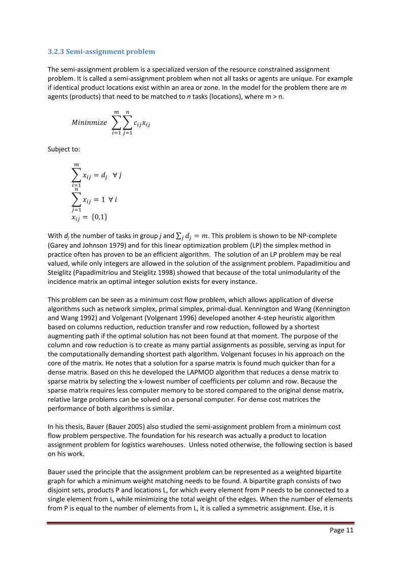
3.2.3 Semi-assignment problem The semi-assignment problem is a specialized version of the resource constrained assignment problem. It is called a semi-assignment problem when not all tasks or agents are unique. For example if identical product locations exist within an area or zone. In the model for the problem there are m agents (products) that need to be matched to n tasks (locations), where m > n.
𝑀𝑖𝑛𝑖𝑛𝑚𝑖𝑧𝑒 ��𝑐𝑖𝑗𝑥𝑖𝑗
𝑛
𝑗=1
𝑚
𝑖=1
Subject to:
�𝑥𝑖𝑗
𝑚
𝑖=1
= 𝑑𝑗 ∀ 𝑗
�𝑥𝑖𝑗
𝑛
𝑗=1
= 1 ∀ 𝑖
𝑥𝑖𝑗 = {0,1} With dj the number of tasks in group j and ∑ 𝑑𝑗 = 𝑚𝑗 . This problem is shown to be NP-complete (Garey and Johnson 1979) and for this linear optimization problem (LP) the simplex method in practice often has proven to be an efficient algorithm. The solution of an LP problem may be real valued, while only integers are allowed in the solution of the assignment problem. Papadimitiou and Steiglitz (Papadimitriou and Steiglitz 1998) showed that because of the total unimodularity of the incidence matrix an optimal integer solution exists for every instance. This problem can be seen as a minimum cost flow problem, which allows application of diverse algorithms such as network simplex, primal simplex, primal-dual. Kennington and Wang (Kennington and Wang 1992) and Volgenant (Volgenant 1996) developed another 4-step heuristic algorithm based on columns reduction, reduction transfer and row reduction, followed by a shortest augmenting path if the optimal solution has not been found at that moment. The purpose of the column and row reduction is to create as many partial assignments as possible, serving as input for the computationally demanding shortest path algorithm. Volgenant focuses in his approach on the core of the matrix. He notes that a solution for a sparse matrix is found much quicker than for a dense matrix. Based on this he developed the LAPMOD algorithm that reduces a dense matrix to sparse matrix by selecting the x-lowest number of coefficients per column and row. Because the sparse matrix requires less computer memory to be stored compared to the original dense matrix, relative large problems can be solved on a personal computer. For dense cost matrices the performance of both algorithms is similar. In his thesis, Bauer (Bauer 2005) also studied the semi-assignment problem from a minimum cost flow problem perspective. The foundation for his research was actually a product to location assignment problem for logistics warehouses. Unless noted otherwise, the following section is based on his work. Bauer used the principle that the assignment problem can be represented as a weighted bipartite graph for which a minimum weight matching needs to be found. A bipartite graph consists of two disjoint sets, products P and locations L, for which every element from P needs to be connected to a single element from L, while minimizing the total weight of the edges. When the number of elements from P is equal to the number of elements from L, it is called a symmetric assignment. Else, it is

Page 12
asymmetric. For an asymmetric case no perfect matching exists, as some elements of L remain unmatched (when |L| > |P|). The symmetric and asymmetric assignment problem also can have subset constraints, where L is partitioned into various disjoint subsets L1, L2, … , Ls for which each has capacity li. From this, two cases can be distinguished: strict capacity constraints where ∑ 𝑙𝑖𝑠
𝑖=1 = |𝑃| and loose capacity constraints where ∑ 𝑙𝑖𝑠
𝑖=1 > |𝑃|. In the former case the number of assigned products must match the number of locations available for all subsets Li, while in the latter case fewer products than locations can be assigned to a subset. Because the number of assigned products per subset is not known in advance for the problem with loose constraints, the problem is harder to solve. A problem with loose constraints can be turned into one with strict constraints by introducing dummy products with demand or pick cost 0. The problem with loose constraints is a generalized version of the one with strict constraints. The cases that Kennington & Wang, and Volgenant studied were both symmetrical problems. Bauer studied the effectiveness of several algorithms in finding the optimal solution for an asymmetric constrained assignment problem that are faster than the generic flow algorithm. He compares the results of an ‘auction with heap’ and a ‘forward/reserve auction’ algorithm with a virtual nodes algorithm developed by Unterhofer (Unterhofer 2003). The auction algorithm with heap implementation is a heuristic primal-dual algorithm introduced by Bertsekas et al. (Bertsekas, Castanon et al. 1993) and its working resembles an auction where the people (products) bid for objects (locations) by increasing their price with small steps. This is implemented using a heap with |L| nodes rather than a full size cost matrix. The forward/reserve auction algorithm was proposed in the same article by Bertsekas et al., but in this case the objects also compete for a person by lowering their prices. The virtual node algorithm by Unterhofer converts the asymmetrical problem into a symmetrical one by adding |L| - |P| nodes on the right hand side, connected with every other node on the left hand side with cost 0. Then the auction algorithm of Bertsekas et al. is applied to this symmetric problem. Both algorithms proposed by Bauer are competitive with, but in many cases better than, the virtual nodes algorithm. Between the two, forward/reserve is often faster than the auction with heap, but requires more computer memory. So the choice is dependent on whether if computer memory is a limiting factor or not. Dell’Amico and Toth compared 8 algorithms for solving the linear assignment problem. In their benchmark study (Dell'Amico and Toth 2000) they showed that the three auction based algorithms (auction forward/reserve, auction floating point and naïve auction) are not competitive to the other ones when solving dense matrices. Dependent on the case either LAPMOD from Volgenant, the shortest path from Jonker and Volgenant or the Goldberg and Kennedy double-push algorithm is the best performing algorithm. It does need to be noted that this was only tested for symmetrical linear assignment problems with strict constraints, thus making it difficult to assess whether auction based algorithm would perform better in the case studied by Bauer.
3.2.4 Categorized bottleneck assignment problem The categorized bottleneck assignment problem (CBAP) is a generalized version of two models. The problem can be described as the assignment of m jobs (products) to n machines (zones). If n = 1, it is equal to the classic assignment problem with the objective to minimize the total cost. If n =m, it becomes the bottleneck problem with the minimax objective from Ford and Fulkerson from Section 3.2.1. In general form this problem is written as:

Page 13
𝑀𝑖𝑛𝑖𝑛𝑚𝑖𝑧𝑒 max1≤𝑗≤𝑛
�𝑐𝑖𝑗𝑥𝑖𝑗
𝑚
𝑖=1
Subject to:
�𝑥𝑖𝑗
𝑚
𝑖=1
= 𝑘𝑗 ∀ 𝑗
�𝑥𝑖𝑗
𝑛
𝑗=1
= 1 ∀ 𝑖
𝑥𝑖𝑗 = {0,1} With i = {1,2,..,m} the products to be assigned to zones j = {1,2,..,n} with capacity kj. The formulation is adapted from Burkard (Burkard, Dell'Amico et al. 2009). Unless m = 1 or m = n, this problem is strongly NP-hard (Punnen 2004). The problem resembles the semi-assignment problem from the previous section, but only differs in the objective function. It is also similar to the multiple bottleneck assignment problem (MBAP), also studied by Punnen and Aneja (Punnen and Aneja 1993, Aneja and Punnen 1999) amongst others. Although MBAP is considered a scheduling problem rather than an assignment problem, the algorithms proposed for that type of problem can also be considered for CBAP. For CBAP a heuristic algorithm was developed by Aggarwal, Tikekar and Hsu (Aggarwal, Tikekar et al. 1986). Originally it was presented as an algorithm able to find the optimal solution, until it was proven by Punnen (Punnen 2004) that the problem was NP-hard. Unless P = NP, the algorithm will provide a near-optimal solution. The focus of their algorithm is a reduction procedure to obtain a sharper bound for the branch and bound algorithm when tasks assigned to a machine have to be processed in series. This resembles the assignment of products to pick zones or racks and summing the associated cost per pick zone. Aneja and Punnen developed two algorithms to find a near-optimal solution. In their article published in 1993 (Punnen and Aneja 1993) they study MBAP when the assignments are split in various groups and the tasks in these groups have to be processed in series. They present a greedy algorithm of which the results serve as input for a tabu search algorithm. With this method they produced some promising results as the tabu algorithm improves the result of the greedy algorithm considerably, but a disadvantage is the O(n2log r) running time of each tabu iteration. In their later article (Aneja and Punnen 1999) they use a subgradient optimization procedure to obtain a sharper lower bound that can be used in a branch and bound algorithm. Although it defines a sharper bound compared to other algorithms, they did not test the algorithm to quantify the speed gained in solving the problem.
3.3 Literature conclusions In the literature no references have been found to a similar problem as the one being studied in this thesis. The problem studied by De Koster and Yu (De Koster and Yu 2008) has a side constraint similar to the Family-to-station constraint in this problem. Their two-phase algorithm is not suitable for this problem to obtain near optimal results because of the moves restriction. It would be able to generate a feasible start solution relatively fast as it divides the problem into seven sub-problems: one family to station assignment problem and six product to zones assignment problems.

Page 14
The assignment problem in various shapes and forms has been subject of study for many researchers. The problem formulation that comes closest is the Categorized Bottleneck Assignment Problem with Ford and Fulkerson’s minimax objective and 1 ≤ m ≤ n. This problem is formulated with strict capacity constraints and is classified as NP-hard (Punnen 2004). Bauer (Bauer 2005) indicated that the problem with loose constraints is harder to solve than the one with strict constraint. Thus this adds to the complexity of the problem. Because of this, it is not realistic to think that the optimal solution will be found in reasonable time. Heuristics need to be used to find a near optimal solution within a reasonable amount of time. Because no literature has been found that deals with the family-to-station, power sequence and moves constraints, it is unclear how this affects the problem and the ability to find a (near optimal) solution. The standard cost minimization objective minimizes the total picking cost over the entire area, but allows for large variation between zones. It is the desire of Valeant, and supported by research from Jane (Jane 2000) and Yu and De Koster (Yu and De Koster 2008), to balance workloads between zones. With Ford and Fulkerson’s minimax objective the objective is to prevent zones with excessive high workloads. Martello’s objective criteria minimize the difference between the zones with the highest and the lowest workload. The latter is the desired objective function, but might be more difficult to implement compared to the former. Various heuristics have been used to tackle this problem. Some were created for specific situations, but the most frequently used generic algorithms for resource constrained problems are variable or Lagrange relaxation, tabu search and branch and bound. Branch and bound is no heuristic by itself, but heuristics are use to determine the upper and lower bounds of nodes.

Page 15
4. Methodology At the basis of scientific research stands a sound research method. The methodology applied in this thesis is described in this chapter. First the problems that can be encountered while preparing for or executing the analysis are discussed, followed by an overview of the tools used and setting applied to these tools. Data collection and preparation is discussed in Section 4.3. Section 4.4 describes the analytical procedure that is applied and some of the choices made.
4.1 Problems Several problems or risks need to be considered when performing the analysis. When not properly assessed, they can complicate the analysis or the ability to find an acceptable solution. Problem complexity Despite the continuous increase of CPU speeds and computer memory, NP-hard mixed integer LP problems remain practically solvable for relatively small instances only. For the assignment of 20 products already more than 2.3*1018 solutions are possible. If a computer was able to compute 1,000 solutions per second, it would still take more than 77 million years to review all options. Based on this, it can be assumed that the assignment of 2,659 products to a location, which is the subject of this thesis, is not considered to be a small instance. Next to that, computer memory can be a limiting factor for some algorithms. For example, node trees for large problems require more space then what is available for memory. Valeant requires the algorithm to be run on a normal desktop computer or laptop with 4 GB of memory. For these reasons it will be close to impossible to find the optimal solution for this problem. However, it may be possible to find a near optimal solution. Algorithms As shown in Chapter 3, several algorithms have been developed in the past 50 years for specific instances of the assignment problem to generate near optimal solution within an acceptable time. However, it is unclear how these algorithms perform on this specific case because no references were found to a problem with identical side constraints as the one currently under investigation. It could be possible to adapt, implement and test all these algorithms for this problem but this would take a considerable amount of time with no clear expectation of the results. This falls therefore outside the scope of this thesis. Starting assignment With an almost unlimited number of solutions available, an identical number of starting assignments can be generated. To be able to draw solid conclusions from the results and for a method to be scientifically sound, it should be tested on various scenarios and thus various starting or current assignments should be used. However, only one actual assignment from WMS is available: from 22 May 2015. In theory the model could work very well in this instance, but might perform differently with another scenario. Parameter settings The performance of a model also depends on the settings of parameters and algorithm options. The defined model contains one variable that may impact the performance of the algorithm: big-M. The parameter needs to have a sufficiently large value in order to turn on or off the enforcement of a constraint. It is unclear whether it makes a difference to the speed and performance of the model whether the parameter’s value is set to the required minimum or to a very large value. Next to this parameter, the settings of the algorithm parameters can influence the behaviour of the algorithm and thus can have an impact on the performance.

Page 16
4.2 Tools and settings Below is a short description of the software and algorithms used to conduct the analysis to find a method that produces an acceptable solution. Also the settings that are changed from the default value are discussed to allow for reproducibility. Software AIMMS modelling software version 4.1 is used to run the model on because of its wide variety of algorithms suitable for Mixed Integer Linear Program (MILP) problems. The software is run on a Dell laptop with an Intel i5 CPU quad core M520 with 2.4GHz and 4 GB RAM, for which 1,600 MB is available for AIMMS. Ten gigabyte is available on the hard disk for node files. Algorithms The initial optimizer used is CPLEX, relaying in part on the simplex algorithm. The CPLEX implementation of the simplex method was done by Robert Bixby (Bixby 1992). Using CPLEX often relative good results can be obtained within a limited amount of time for MILP. It applies branch and bound techniques and can handle relaxation of the variables and/or constraints, which were frequently used in cases discussed in Chapter 2. For this specific reason is CPLEX chosen as the starting algorithm for this analysis. Tabu search, a meta-heuristic optimization algorithm developed by Fred Glover, can be accessed through AIMMS with the use of AIMMSlinks. This algorithm will be used when CPLEX does not provide acceptable results. If Tabu does not provide acceptable results, other specialized algorithms mentioned in Chapter 3 can be implemented. Heuristics are used to obtain a good and near optimal solution for large instances of integer problems, because it is not possible to calculate and compare every solution. Problems with integer variables are harder to solve compared to continuous variables. One popular and smart technique is branch and bound. For some integer problem types, such as knapsack and traveling salesman problem, large instances with more than 10,000 variables have been solved effectively using branch and bound techniques. This technique branches or partitions the set of solutions in smaller sets and checks these one at a time for a feasible solution that is better that the current best solution, called the incumbent. Effective branch and bound algorithms are computationally very efficient and are able to produce a high quality lower bound, (i.e. a lower bound as high as possible, or close to the minimum objective value in the subset (Murty 1994) for each subset. This speeds up the pruning process during which subsets are evaluated and either accepted because it improves upper bound or discarded. One of the most important strategies for constructing a lower bound is by means of relaxation. With this strategy one or more hard or difficult constraints are relaxed. According to Murty, a constraint is considered to be hard if the relaxed problem can be solved easier if the hard constraint is dropped. The thought behind this strategy is that all solutions from the subset of the original problem are included in the subset of the relaxed problem. If the lower bound of the relaxed subset can easier be obtained, all subsets can be assessed quicker. Relaxation can also be applied to the variable values. By allowing certain or all variables to take on fractional values rather than binary values, the problem can be solved much quicker. However, products in reality cannot be assigned on a fractional basis and the fractional values need to be rounded to integers. Thus the solving of the problem might be quicker, an additional algorithm is required to create a feasible solution. The idea is that a solution with fractional values could be a good starting point for creating such a feasible solution. Software and algorithm settings There are many parameters in AIMMS that control the behaviour and the performance of the program and the algorithms it uses. IBM, the current owner and developer of CPLEX, recommends using the default settings as it works well on most problems. Otherwise the automatic tuning tool,

Page 17
the probing parameter and the MIP emphasis parameter can be changed, amongst others (IBM 2005). The default settings will be used initially, except for the settings described below.
• The maximum run time for each model is set to 8 hours, unless specified otherwise. • When solving small models to optimality the MIP relative optimality tolerance is kept at the
default value of 1e-13. For full size problems, the relative tolerance is set to 0.01, or 1%. This value is chosen so it is well below the minimum threshold of 5%, but will not unnecessarily extend the run time of the model trying to find a solution that is marginally better.
• The MIP ‘advanced start’ parameter is set to ‘use advanced basis’. This way it uses the current assignment as input, rather than trying to create a new assignment from scratch. For this setting is chosen due to the fact that the model is bound by a number of moves it can execute.
• The nodes files are compressed and stored on hard disk. Because of the size of the model (more than 300,000 variables for the full problem), the branch and bound tree will expand quickly beyond the available RAM for the program of 1.6 GB. The compressed node files are allowed to take up to 10 GB of space on the hard disk. The tree memory limit for the RAM is set to 128 MB, per recommendation from IBM, so enough RAM is left for post-solving and other process steps.
• The value for the ‘random seed’ parameter is changed when multiple runs of the same scenario need to be executed to obtain an average value for the root node processing, run time and root incumbent without rebooting the computer. The range of this parameter is from 0 to 2.1e09. No fixed set of values is specified for this parameter.
Several settings have been changed to expand the amount of data written to the log file to assist in analyzing the result. This could have a negative impact on the performance of the model, but these settings will not be changed throughout the analysis phase.
4.3 Data collection The data used for this analysis is supplied by Valeant. The following data is used and extracted from the Oracle WMS-database using SQL:
• Product data such as product family and sequence within the family. The product codes have been replaced by family (p) and sequence (q) indicators to both fit the model and make the data suitable for publishing.
• Current assignment of product within the PTL-area. A product has at most 1 static assignment and can have 0 or 1 dynamic assignments. First all assignments for static locations are collected and to this the assignment from dynamic locations are added that do not have a static assignment. The assignment as on 22 May 2015 is used for validation. An alternative assignment with a high workload deviation between zones was generated for analysis. The set up and the reasons why this alternative assignment was created are discussed below.
• The number of picks per product for a six month period, from September 2014 through February 2015. Only those products are selected that have an active assignment on the day the data was downloaded.
• The number of locations per zone and rack type. Each location belongs to a section. From the section ID the station number (i), zone number (j) and type of rack (k) are derived and aggregated.

Page 18
4.3.1 Alternative assignment The downloaded assignment of 22 May 2015 shows some inconsistencies with the constraints of the model. Changes have been made to the assignment since the last update was executed over one year ago. These changes have been made for practical operational reasons. For example, 85 products are not stored in the station where the majority of their product family is stored. This causes the original assignment to be infeasible. Of the available moves, 85 will be used to find a feasible solution. This is an undesired side effect as it is unknown what the effect is of starting with an infeasible solution on the performance of an algorithm. For this reason a feasible start assignment is generated. The algorithm for creating this start assignment is rather simple. Family 1 is assigned to station 1, family 2 to station 2,…., family 7 to station 1, and so on. Within a station the first 16.7% of the products (in ascending order) are assigned to zone 1, the next 16.7% to zones 2, etc. The first couple of products assigned to a zone, equal to the number of flowrack locations available, are assigned to the flowrack. The remaining products are assigned to the backrack. In general this creates a feasible solution, but in a small number of cases the number of product assigned to the backrack exceeds the capacity. This is solved by hand by assigning products to a higher or lower zone. Comparing the downloaded assignment with the alternative assignment, it can be seen in Figure 2 that the demand distribution differs. The created assignment results in a higher variation in demand between zones. The Mean Average Deviation for the original assignment is 9,953, while that for the created assignment is 23,144.
Figure 2: comparison of starting product assignments with effect on workload per zone. A potential side effect of this created assignment with high deviation between zones could be that the algorithm can decrease the workload first by moving products between zones and racks, rather than between stations. This is not deemed to be a negative side effect as there is no preference for the type of moves that is generated.
4.3.2 Scaled model A reduced version of the original data set is created for analysis. Performing all analyses on the original data set with 2,659 products problem is not sensible as early tests have shown that it either takes a couple of hours or that the program has ran out of memory before useful results are

Page 19
available. No conclusions could be drawn from these results. Therefore, a model is created in Excel that reduces the original data set to a desired size. In this scaled model the original relationships between products has been retained as much as possible. A description of the steps taken to build the scaled model and data set is discussed next. Determining family category In the downloaded assignment 59 product families are assigned to the PTL-area. The number of products per family ranges from 1 to 65. Product families with an equal number of products most often show the same demand pattern within the product family. For this reason, families are grouped based on the number of products they have. Families with less than 25 products were excluded. The demand for these families combined was 0.8% of the total and would not add much to the complexity of the problem. From the original 59 families 52 remain and these were classified into 5 categories, which is shown in Table 1. Figure 3 shows the demand distribution for each product family category.
Family size Number of families Picks Picks %
31 19 61,934 3.9%
44 3 50,095 3.1%
57 5 172,504 10.8%
65 8 414,377 26.0%
69 17 883,148 55.4% Table 1: scaled model classification and distribution of picks for product families.
Figure 3: demand distribution (in picks) per product family category. Scaled model The number of product families and the size of the families are determined by two parameters: problem size and family size. The first determines the total number of products required for the scaled data set and the second determines what percentage of the original number of product per families the scaled families should be. This provides the user the option to reduce the problem size, but also to increase or decrease the relative family size. This allows for investigation of the effect of family size on the solving time of the problem.

Page 20
The demand is distributed over the number of products required for the scaled family. By grouping similar families into categories and assigning the same demand pattern to each family of that category, the variation between families in the same category is lost. In the Excel model the user has the option to introduce demand variation between families of identical size between an upper and a lower bound. The bound is expressed as a percentage of the total.
4.4 Outline of research The problem is NP-hard and these types of problems are only solvable to optimality within an acceptable run time for very small instances. AIMMS is already not able to solve a problem instance with only 77 products distributed over 36 zones, or 3% of the original problem size, to optimality within 8 hours (LP-IP gap is 0.62%). In this case, the maximum number of moves allowed is set to 80, which in fact relaxes this constraint. If for such a small problem instance it cannot be solved to optimality within the given time frame, it is impossible to expect this of a problem that is 30 times bigger. However, the problem does not need to be solved to optimality to get an indication on how the model behaves or how good the solution will be. Explorative analysis has shown that the optimal solution is found already within a relatively short amount of time, after which the branch and bound algorithm explored all remaining branches to validate whether it is indeed the lowest solution. Already at the root of the branch and bound tree important information can be found.
4.4.1 Root node analysis The assumption is that the root node processing time together with the difference between the value of the LP-problem and the root incumbent are a global indicator of the complexity of the problem. Based on this assumption, different methods or algorithms can be compared based on the time it takes to process the root node as this is done for every MIP problem. CPLEX first it solves the LP-problem by relaxing the variables and then processes the root node of the branch and bound tree. The value of the objective function of the LP problem (LP-value) is the best solution possible. The optimal value for the (M)ILP problem (IP-value) will be equal or larger than the optimum of the LP problem. The gap between these two values is defined as the LP-IP gap. At the end of the root node processing a first incumbent for the MIP problem is (usually) found. This is referred to as the root incumbent. The IP-value lies between the LP value and the root incumbent. The gap between the LP-value and the root incumbent is also an indication of how close the initial solution is to the optimum. The focus of the analysis is on the root node processing time and the LP-root incumbent gap. The LP-root incumbent gap and the LP-IP gap are defined as:
The LP-IP gap: (𝐼𝑃 − 𝐿𝑃)
𝐿𝑃∗ 100%
The LP-root incumbent gap: (𝑖𝑛𝑐𝑢𝑚𝑏𝑒𝑛𝑡 − 𝐿𝑃)
𝐿𝑃∗ 100%
4.4.2 Selection of scaled model With the problem scaling tool many combinations are possible. The scaling of the family size also has an impact on the behaviour of the model. If the families are relatively large, there are fewer families but they consist of more products. In theory the model can then be more influenced by the power sequence constraint, than on ‘Family to station’ constraint. If the families are relatively small but there are more of them it could be the other way around. Since the problem is solvable for small instances only, in general the choice has been made to keep the families relatively large to be able to analyze the effect of the ‘Power sequence’ constraint and to make sure that families do not consist of

Page 21
only 4 products. As the 6% is shown to be largest problem size that could be solved to optimality within 4 hours, this will be the basis problem size. The relative family size is set to 16% in which case the majority of the families consist of at least 7 products. This guarantees that for most families at least one zone is assigned two or more products. This is deemed important to stay close to the full problem size. Internal analysis to which was refereed in chapter 1 has sown that, in general, up to 80% of the backrack locations can used for static product assignments. The limits for the zone capacity constraints are set to 80% of the capacity for backracks, unless noted otherwise. This also applies for the scaled model.
4.4.3 Verification and validation The model specified in Chapter 3 is built in AIMMS. To verify whether the model is properly built and complies with the theoretical model, the model is tested on very small problem instances for which it is easy to check whether the model produces the right result. The zone capacity constraint, the maximum moves constraint and the ‘Power sequence’ constraint were first tested on a problem consisting of one station with 2 zones. If these constraints were applied correctly, the model was expanded to two stations with two zones each to check for the ‘Family to station’ constraint. When all constraints were applied correctly the model was expanded to two stations with six zones each for a final check. The question is whether the conclusions drawn from the scaled problem also apply to the full size problem. The increased size of the problem can lead to different dynamics within the model for which the scaled problem is not a proper indicator. This cannot be ruled out. However, the behaviour of the model at the root node for the scaled problem will be compared with that of the full size problem. If these align or show a similar behaviour, it is assumed that the models behaviours are similar when solving to optimality. The results from the model are validated by executing at least two runs of the same case, but for different random seeds. This is done because CPLEX and branch and bound are heuristics for which the run time and/or result can differ per run. This also prevents that conclusions are drawn based on the results of a single, very positive or very negative, run. Unfortunately, due to time restriction and the fact that the run time per case is up to eight hours, in most cases not more than two runs were executed per case. This poses a risk for the validity of the results, but it is believed that the results are clear enough to draw conclusions from. The final model is validated using a new data set. Most analysis is done on a scaled problem that is derived from the original problem. The demand is the actual demand over the past size months, from May through November 2014, but the assignment was created by hand to introduce a high variation between the zones. The final model is validated using the actual product assignment from May 22nd, 2015.

Page 22

Page 23
5. Results This chapter presents all the results from the analysis and experiments conducted based on the methodology described in Chapter 4. In Section 5.1 a change in objective function is presented with the reason for this change. The effect of the unique combination of side-constraints is discussed in Section 5.2. Whether a feasible and acceptable solution can be obtained with decreased model run time by relaxation of variables and fractional rounding is the subject of Section 5.3. This is followed in Section 5.4 by a study into the effects of the value for big-M. The last section, Section 5.5, presents the final model applied to the generated and the downloaded assignment.
5.1 Objective function Implementation of the objective function that minimizes the difference between the zones with highest and the lowest workload proved to be very difficult for this ILP problem. The combination of side constraints with the objective function to minimize the deviation in zone workload made the model non-linear. This increases the complexity of the already complex model. On top of that, AIMMS is not able to deal with big-M constants in a non-linear model mixed integer problem. Since this is a key element of the problem, the choice is made to change the objective function to the Ford and Fulkerson’s minimax objective function. With this objective function the model behaves linear and big-M constants or indicator constraints can be applied. The aim now becomes to minimize the highest zone workload and the objective function thus becomes:
min𝑖,𝑗
���𝐷𝑝𝑞𝑥𝑖𝑗𝑘𝑝𝑞𝐿𝑘𝑞𝑝𝑘
It is expected that the resulting workload variance between zones will not differ much from when the minimized variance objective function would be used. When there are no zones with an exceptionally low workload, the difference will be minimal. Next to that, when a low number of moves is allowed, the desired behaviour from a practical perspective would be to reduce the zones with the highest workload rather than increase the workload for the zones with the lowest. Since the original objective was to measure the difference between zones, an additional criterion is introduced: Mean Absolute Deviation (MAD). This is defined as:
𝑀𝐴𝐷 = 1𝑛∑ |𝑥𝑖 − �̅�|𝑛𝑖=1
This metric will be used next to the maximum zone workload, to which the model optimizes, to assess the effectiveness of a solution.
5.2 Effect of side constraints The model is bound by this set of side constraints:
• Zone capacity constraint • Move constraint • ‘Family to station’ constraint (Station) • ‘Power sequence’ constraint (Power)
The zone capacity constraint is a relative familiar constraint. The way it is defined in this thesis, it can also be found in the semi-assignment with loose capacity constraints. For the other three however no reference was found in literature. The effect of the three constraints on the performance of the

Page 24
model is studied using root node processing time and the LP-root incumbent gap (see Section 4.4.1 for definitions).
5.2.1 Station and power constraints First, the effect of the Station and Power constraints is tested. The move constraint is effectively relaxed by setting the maximum number of moves to equal or larger than the number of products available. The zone capacity constraint is active for every problem with 80% of the backracks available for static product assignments. In Figure 4 for several problem sizes the average root node processing times are plotted for the four possible combinations of the constraints: both applied, Station only, Power only and none. It shows that the time for the two models with Power constraint increases exponentially for increasing problem sizes compared to when it is not applied. Also, processing the root node of the full size problem with Power constraint takes on average 29 minutes, compared with 4 minutes when the Power constraint is dropped.
Figure 4: average root node processing times for four combinations of constraints and various problem sizes (at least 2 runs per data point). Table 2 shows the results for the two scenarios for the full size problem with Power and Station constraint applied. Scenario 1 is the scaled model with the problem size set to 100%, the family size set to 100% and generated start assignment. Scenario 2 is the original download from WMS with the original family sizes and demand per product, but with generated start assignment. For both scenarios an incumbent was found at completion of the root node processing, however the incumbent is not close to an acceptable solution. Even after 8 hours the gap with the LP-value is still at least 38.9%. Another observation from the table is that only 209 and 101 nodes, respectively, in the branch and bound tree have been generated. This means, that for scenario 1 it on average takes 138 seconds to process a node. This is too long in order for a branch and bound algorithm to be effective. Based on these results, it is not possible to generate an acceptable solution within 5% of optimality and within the desired time with all constraints applied. Scenario LP-
value Root incum-bent value
Final incum-bent value
Final gap
Number of incumbents
Nodes
1 49754.5 82858 82147.5 65.1% 2 209 2 44199.6 82011 61387.5 38.9% 2 101 Table 2: overview of results for full size scenarios with Power and Station constraints after 8 hours.

Page 25
The LP - root incumbent gap for the model without Power constraint is already less than 20% (10.6% for scenario 1 and 19.7% for scenario 2) and provides a more promising basis for the branch and bounding during the remaining time. These findings with respect to the Power constraint were presented to Valeant. From a separate analysis conducted around the same time the result was that only a couple of customers are still demanding that their products are delivered in power sequence. Valeant concluded that the benefits are no longer greater than the cost and the restrictions that come with it. Therefore they decided to drop the Power constraint for a test period of three months. The power sequence packing service will still be provided to customers who want it, but will be charged for it. If the error rate and the number of complaints do not rise during the test period, the power picking sequence service will stay off. Based on this, the Power constraint was dropped from the problem. This does not make the model solvable to optimality, or close to it, within 8 hours. With the moves constraint relaxed (set to 2,700 moves), AIMMS runs out of working memory towards the end while the gap between the LP and incumbent values is still larger than 5% for both scenarios.
5.2.2 Maximum moves allowed Another constraint for which it is unclear what the impact is on the model is the maximum number of moves allowed. Figure 5 below shows the solution gap at the root node between the LP and the root incumbent as well as the root node solving times for the full size problem in relation to the number of moves allowed. The values are measured for 100 moves intervals, the variables can only take on binary values and the Power constraint is dropped.
Figure 5: average solution gap at root and average rote node processing times for full problem vs number of moves allowed (2 runs). Three observations are made from this figure. First, up to 900 moves the optimal solution of the LP is bound by the number of moves that can be executed. The LP solution does not further improve after 900 moves, meaning that in theory the optimal solution can be reached by moving only a third of the products. Secondly, the LP – root incumbent solution gap is quite large. The gap varies between 18.4% and 35.8% and thus is not yet close to an acceptable solution. The last observation is that the root node solving time is relative constant around 200 seconds, except for the interval between 200

Page 26
and 700 moves allowed. The reason for the increased solving time in this interval is unclear, as well as for the steep drop off in solving time between 700 and 800 moves. Dropping the Power constraint simplified the model and made it possible to solve it to optimality for the 6% scaled problem. In this scenario the problem has 156 products distributed over 19 families. The family size parameter is set to 16%. Figure 6 shows the LP, IP and average root incumbent values. The LP – root incumbent gap range from 33.7% to 88.4%, in part due to three large average incumbent values at 120, 130 and 160 moves. For 10 and 20 moves, the root incumbent eventually proves to be the optimal value. From 40 moves onward, the IP solution is roughly in the middle between the LP and root incumbent and is around 20% higher than the optimal value for the LP problem. The optimal IP value is already reached by executing 50 moves, or a third of the products. This is on one hand encouraging. On the other hand the run time for this range of moves is expected to be longest.
Figure 6: LP, IP and average root incumbent value for 6% scaled problem size with 16% family size (3 runs).
Figure 7: average root node processing and average problem solving times for MIP problem at 6% or original problem (3 runs). Comparing the root node processing time and total run time when solved to optimality for the 6% problem, a striking observation is made. Figure 7 shows that there appears to be an exponential

Page 27
relation between the two. The root node solving time is plotted on the primary y-axis on a normal time scale, while the total run time is plotted on the secondary y-axis in a logarithmic scale. If this exponential relation would apply in general, the root node processing time would be a very good indicator for whether the problem can be solved to optimality within the desired time frame. Also, the root node processing time for the 6% problem has a similar pattern as for the full size problem from Figure 5. Which also supports the idea that conclusions or observations made for the 6% scaled problem would apply to the full size problem.
5.3 Relaxation of variables In an attempt to find an acceptable solution quicker relaxation is applied. The constraints can be relaxed or the variables. Relaxing the right constraints can make it easier for the branch and bound algorithm to find a lower bound for a branch and thus potentially speed up to the solving process. This is called Lagrange relaxation. First the possibilities by relaxing variables are studied. The variables can be relaxed by allowing one or more variables to take on fractional rather than just binary values. This transforms the problem from an ILP to an MILP or LP problem, which in general should be easier to solve. The solution of the MILP and LP problems could provide a good basis for a solution using fractional rounding techniques. The ‘postsolve integer variables’ option is changed from ‘Round integers and resolve LP’ to ‘No rounding’ to prevent that the variables are rounded to integers at the end. First the LP problem is studied, then the MILP.
5.3.1 LP problem To transform the ILP into an LP problem, the domain of the variables xijkpq, xip and mijkpq is changed from {0,1} to [0,1]. The problem is then solved to optimality within a minute on average. Because of the short run time of the model, the results of the full size model are studied in this section. To start on a positive note: more than 97% of the assignment variables xijkpq are, or remain, an integer. On a negative note, the Station constraint is not effectively applied. Because the Station constraint contains a variable, xijkpq and xip, at each side of the equation, for all combinations of xijkpq a combination for xip exists for which the constraint is valid. The proof is easy to generate and is not shown here. As a result, products families can be assigned to multiple stations. A feasible solution, with Station constraint effective, is generated from the fractional solution by applying fractional rounding twice. First, on variable xip by rounding the highest value xip for every p to 1, while setting all others to 0. The corresponding variables for xijkpq are updated accordingly: all products from a family are assigned to the station for which now xip = 1. Then all variables xijkpq with fractional values are rounded up or down. The highest value of xijkpq for every p,q combination is rounded up to 1, all others are set to 0. This process usually does not generate a feasible solution, as the zone capacity constraint is violated for several zones. A major drawback of this method is also that the moves constraint is violated. Due to rounding of both variables in most case more moves are generated than allowed via the maximum allowed moves parameter. Table 3 shows the results for up to 1,000 moves. From 1,100 moves onward, the move constraint is not violated for the two-step rounded solution, but the zone capacity constraint is. Figure 8 shows the MAD development for the two-step rounded solution (with violated zone constraints) for the original problem with generated assignment. The MAD for 0 moves is the MAD of the start assignment. To create a feasible solution from the rounded LP solution, the problem becomes again an IP problem where families are kept together in stations and zone capacity constraints need to be maintained. This can be solved by a model that optimizes the workload per station, in fact creating a two-phase optimization model like the model from De Koster and Yu (De

Page 28
Koster and Yu 2008) discussed in Chapter 3. Workload balancing between zones in a station will generate additional moves and thus will even further violate the moves constraint. Moves allowed Moves generated Zone violations Variable integer %
100 98 3 98.8% 200 199 12 98.2% 300 312 17 97.7% 400 427 15 97.6% 500 530 16 97.4% 600 634 15 97.6% 700 729 17 97.6% 800 806 16 97.6% 900 905 18 97.4%
1,000 1,007 22 97.3% Table 3: selected results of LP problem with two-step fractional rounding for 100 – 1,000 moves.
Figure 8: development of mean absolute deviation for two-step rounded LP problem.
5.3.2 Partially relaxed variables Allowing the variable xip to take on binary values only, while the other two variables can take on fractional values, the problem becomes a MILP problem that could provide the best of both worlds. The binary variable will keep the products families together in the same station, while the fractional variables can help to decrease the model run time. It is from here on referred to as the model with partially relaxed variables. This model is again tested on the 6% scaled model, for which every instance can be solved to optimality. Figure 9 shows the LP, IP and average root incumbent values for this model. The IP solution remains relatively close to the LP value: decreasing from 17.0% at 20 moves to 4.8% from 70 moves onward. Not only is the IP value lower when compared with the ILP problem in Section 5.2.2, also the root incumbent is lower. This benefit could be lost as fractional values of the variables in the solution of the partially relaxed model still need to be rounded.

Page 29
Figure 9: LP, IP and average root incumbent values for 6% scaled model with 16% size families and with partially relaxed variables (2 runs). An interesting change compared with the ILP model is the change in root node processing time and model run time in relation to the number of moves allowed. Figure 10 shows that the time for both the root node and the total run time are increasing with the number of moves allowed. This is in contrast with the ILP problem, where the run time was decreasing with increasing number of moves allowed. The model run time is plotted on the vertical axis with a logarithmic scale to see if there is again an exponential relation between the root processing and run time. In this case the relation does not exist or is not as strong as with the ILP problem. Another interesting observation comes from the log files, showing that often the best solution is found already within 2 minutes. As all branches continue to be pruned, the LP value will rise until all branches have been eliminated and the incumbent is accepted as the optimal solution. If the optimal solution is found early on for the full size problem, this could be very advantageous.
Figure 10: average root node processing and model run time for 6% scaled problem with 16% family size for partially relaxed variables (2 runs). The percentage of variables with an integer value in the solution decreases as the number of moves allowed increases. It starts with 87.2% for 10 moves and decreases to 70%. Fractional rounding creates a valid assignment for most non-integer variables: on average only 3 products need to be manually assigned. This is for products that are spread over more than three zones within a station and those will be assigned to the zone with the highest fraction. The fractional rounding and manual assignment creates in a couple of cases zone capacity constraint violations but only in the flowracks. These excess products can be assigned to the backracks as these have enough locations available.

Page 30
5.4 The effect of big-M constant The use of big-M constants is not always preferred. Richards and How state that the use of big-M can make the solution process of MILP harder and recommends investigating whether the problem can be formulated without the use of big-M, as it could be more efficient (Richards and How 2005). Camm et al. show that while often is stated that the value of big-M should be set sufficiently large; it should not be set too large (Camm, Raturi et al. 1990). Rardin states that ‘whenever a discrete model requires sufficiently large big-M’s, the strongest relaxation will result from models employing the smallest valid choice of those constants.’ (Rardin 1998) Even the developers of AIMMS warn that the use of big-M constants ‘can introduce unwanted side-effects and numerical instabilities into a mathematical program’ (Roelofs and Bisschop 2014). They recommend the use of indicator constraints as they are numerically more robust and accurate than conventional formulations for big-M (AIMMS 2015). Thus big-M and its value can have an impact on the performance of the model. In this problem the use of big-M or indicator constraint is inevitable. To assign whole product families to a single station, either the use of big-M or the indicator constraint is required. In this section the effectiveness of these two methods is tested with respect to the performance of the model. Three different scenarios are investigated:
1. AIMMS indicator constraint 2. Big-M with sharp defined constant value (sharp big-M) 3. Big-M with large constant value (loose big-M)
For the first scenario no constant value needs to be defined. For the other two ‘sufficiently’ large values are used. Scenario two is when the boundary for big-M can be calculated for which it shows the desired behaviour as suggested by Camm et al. The last scenario is with a more randomly selected large value for big-M. In this problem the boundary for scenario 2 can be calculated from the Station constraint.
𝑀𝑥𝑖𝑝 ≥���𝑥𝑖𝑗𝑘𝑝𝑞𝑞𝑘𝑗
∀ 𝑖,𝑝
xip takes on binary values, while xijkpq varies between 0 and 1. The maximum value of the right hand side is the number of products from family p stored in station i. Since all products need to be in one station, the maximum value it can take is ∑ ∑ ∑ ∑ 𝑥𝑖𝑗𝑘𝑝𝑞𝑞𝑘𝑗𝑖 , which is the number of products in a family. Thus the big-M value needs to be at least the number of products in product family p. Either big-M can be set to the number of the largest product family, or could be tailored for each product family. In this case the latter is chosen. Big-M is made dependent on p and set to the family size. This is from here referred to as using ‘sharp big-M’. The value of big-M for the loose big-M is set to 1,000. The three scenarios are tested in AIMMS on the full size model, where the program is stopped when a solution within 1% of optimality is found or the maximum run time of 2 hours is reached. The full size model is chosen to see how fast an acceptable solution is found. The model with sharp big-M performs better than the models with loose big-M and the indicator constraint. For up to 900 moves, the Figures 11 through 13 shows the root node solving times, the run times and the incumbent values for the three scenarios. This only done for up to 900 moves as previous results showed that the optimum workload distribution can be achieved by moving only a third of the products. In 7 out of 9 cases the sharp big-M has a faster root node processing time. In all cases the sharp big-M finds an incumbent that is at least as good as the one with the indicator constraint. For 100, 200 or 300 moves allowed the solution is found faster with sharp big-M than

Page 31
with indicator constraint. For 400 to 900 moves the sharp big-M solution is on average 2.2% better than the indicator constraint and the loose big-M is on average 1.1% better.
Figure 11: average root node solving times for three big-M scenarios (3 runs).
Figure 12: average incumbent values for three big-M scenarios at 1% LP-IP gap or after 2 hours (3 runs).
Figure 13: average model run time for three big-M scenarios with 1% LP-IP gap stopping criteria (3 runs). Figures 14 and 15 show the development of the incumbent over time for two cases: 300 and 700 moves. The solutions for the loose big-M and the indicator constraint develop in a similar fashion,
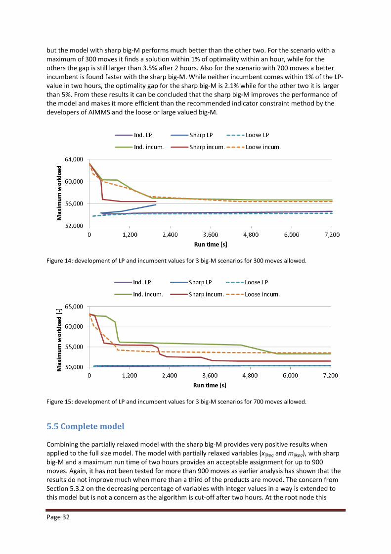
Page 32
but the model with sharp big-M performs much better than the other two. For the scenario with a maximum of 300 moves it finds a solution within 1% of optimality within an hour, while for the others the gap is still larger than 3.5% after 2 hours. Also for the scenario with 700 moves a better incumbent is found faster with the sharp big-M. While neither incumbent comes within 1% of the LP-value in two hours, the optimality gap for the sharp big-M is 2.1% while for the other two it is larger than 5%. From these results it can be concluded that the sharp big-M improves the performance of the model and makes it more efficient than the recommended indicator constraint method by the developers of AIMMS and the loose or large valued big-M.
Figure 14: development of LP and incumbent values for 3 big-M scenarios for 300 moves allowed.
Figure 15: development of LP and incumbent values for 3 big-M scenarios for 700 moves allowed.
5.5 Complete model Combining the partially relaxed model with the sharp big-M provides very positive results when applied to the full size model. The model with partially relaxed variables (xijkpq and mijkpq), with sharp big-M and a maximum run time of two hours provides an acceptable assignment for up to 900 moves. Again, it has not been tested for more than 900 moves as earlier analysis has shown that the results do not improve much when more than a third of the products are moved. The concern from Section 5.3.2 on the decreasing percentage of variables with integer values in a way is extended to this model but is not a concern as the algorithm is cut-off after two hours. At the root node this

Page 33
percentage is around 99% and it slowly decreases over time but not more than 2% over the two hours. When the 1% threshold or the time limit is reached at least 97.5% of the assignment variables have an integer value. Table 4 shows the LP-IP gap and the integer percentage at cut-off. On average 2, but no more than 5, manual assignments need to be made for products that are fractionally assigned to three zones or more. The rounding of variables causes zone capacity constraints violations, but only for the flowracks. Moving the excess products to the backracks solves again this issue, with some impact on the MAD and workload distribution. The effect of these moves on the maximum, average and minimum workload per zone is displayed in Figure 16, and the effect on the MAD in Figure 17. In the latter figure, the MAD for the partially relaxed model is compared with the MAD from the two-step rounded LP model. The values at 0 moves represent the situation from the generated start assignment. It is clear that the relaxed model produces much better results than the LP model. Moves allowed LP-IP gap Integer var. percentage
100 1.0% 99.1% 200 1.0% 98.5% 300 1.0% 97.9% 400 2.1% 97.9% 500 2.3% 97.8% 600 2.5% 97.7% 700 2.1% 97.6% 800 2.7% 97.5% 900 1.5% 97.6%
Table 4: overview of LP-IP gap and integer variable percentage after cut-off.
Figure 16: maximum, average and minimum workload per zone versus number of moves allowed.

Page 34
Figure 17: development of mean absolute deviation versus number of moves allowed for rounded partially relaxed model compared with two-step rounded LP model. The average workload is reduced up to 16.0%, the maximum workload up to 66.6% and the minimum workload is increased with a maximum of 177%. The variation between the zone workload or MAD is reduced with a maximum of 96.6%. For 400 moves the before and after workload distribution is shown in Figure 18.
Figure 18: workload distribution for start and new assignment for 400 moves with partially relaxed model. For validation purposes the model is applied to the actual product assignment of May 22nd 2015. The partially relaxed model is run twice with the same start assignment but for different random seed numbers. The LP, average IP and average root incumbent values are plotted in Figure 19. The minimum number of moves in the graph is 150 as the model is not feasible for 100 moves. This is caused by two things. First, 84 products are stored outside the station where the majority of the products of that family is stored in. Secondly, the zone capacity constraint is exceeded in the start assignment for 5 zones by 22 products in total. Between both sets there is no overlap, thus it takes already more than 100 moves to create a feasible solution. Allowing 150 moves results in a feasible solution but also already in a reduction of MAD with 92.6%. The MAD is maximally reduced with 98% for 700 moves. The development of MAD with the number of moves allowed is depicted in Figure 5.20, together with the maximum, average and minimum zone workload.

Page 35
Figure 19: LP, IP and average root values for validation assignment (2 runs).
Figure 20: average of MAD, maximum, average and minimum workload vs. number of moves allowed (2 runs). On average less than 2 products are not correctly assigned after fractional rounding with the cut-off value set at 0.5. The maximum number of unassigned products for a run is 7. All cases concern products for which fractions are assigned to three stations or more. The assignment can be created by hand for these. On a down side, for nearly every run the zone capacity constraint is violated for at least one zone. This is only for items assigned to the flowracks, with enough capacity available in the corresponding backracks to move the excess flowrack products to. If the product with the lowest demand is moved to the backrack, the MAD increases with up to 2%. Additional moves are required for this and thus the maximum allowed moves constraint is violated in almost all cases.

Page 36

Page 37
6. Conclusions and recommendations Based on the literature research from Chapter 3 and the results presented in Chapter 5 answers to the principal and derived research questions can be formulated. The goal of this study was to find an answer to question: In what ways is it possible to generate a feasible product assignment within 8 hours that is within 5% from the optimal solution, while satisfying the constraints? By relaxing the binary variables xijkpq and mijkpq, thus making an MILP from the original ILP problem, and rounding the fractional variables, the basis for a feasible solution can be generated for problems in excess of 2,659 products using CPLEX and branch and bound techniques. The variables with fractional values are rounded to integer. In all cases for the problem with 2,659 products the 5% threshold was reached within two hours, thus for larger problem instances similar results should be feasible within 8 hours. The size up to which this is possible has not been tested. This conclusion is only applicable for the problem without the Power constraint, as this one was dropped in conjunction with Valeant. The original IP problem with Power constraint could not be solved to optimality within 8 hours for problem instances of 66 products (3% of original problem size) or more. Even without the Power constraint the integer problem cannot be solved to optimality for 2,659 products within 8 hours. It can be done for a problem with 156 products (6% of the original problem size) over 36 zones. For 180 products the solving time for 30 – 50 moves allowed will start to exceed 8 hours. The literature study conducted in Chapter 3 showed that the most frequently used generic algorithms for resource constrained problems are variable or Lagrange relaxation, tabu search and branch and bound. The algorithms from the referenced literature were designed for specific problems, but did not match the constraints applicable for this problem. Partial variable relaxation was tried for this problem and returned good results. The algorithm by De Koster and Yu (De Koster and Yu 2008) appears to be an effective algorithm and could be considered for future research to generated a feasible start solution. Using the partially relaxed model, the maximum number of moves allowed in the model should be set to 5 less than the desired maximum moves one wishes to execute to correct for flowrack zone capacity violations caused by factional rounding. There appears to be no relationship with the number of zones or moves and is caused by fractions of products being assigned to flowrack locations. When more fractions in a flowrack zone are rounded up than down, the constraint is violated. This can be corrected by moving the excess products from the flowrack to the backrack. Experiments have shown that reserving 5 moves is enough for more than 90% of the cases. If this recommendation is applied, it is possible to find a feasible assignment within 8 hours and within 5% from optimality that satisfies all constraints. The three unique side constraints investigated in this thesis all have a different impact on the behaviour of the model. The Power constraint has proved to make the problem much more complex for CPLEX to solve, even though this constraint in theory reduces the pool of potential solutions. Other potential methods that focus on local search techniques such as Tabu or relaxation of variables might provide better results, but have not been studied because Valeant opted to drop the constraint. The Station constraint also adds complexity to the problem, measured in root node processing time, but not as much as the Power constraint. It reduces the pool of potential solutions compared with a problem without Station constraint, but increases the root node processing time. The maximum allowed number of moves has shown a different influence on the root node processing time for two models. The peaks in processing time are at different parts of the spectrum for the ILP and the partially relaxed model or MILP. For the ILP model the peak was found in the first

Page 38
third of the moves spectrum, while for the partially relaxed model it was found in the last third. What caused these differences in behaviour is unclear, and could be subject of future research. Constraint or Lagrange relaxation applied as a method to obtain lower and upper bounds during branch and bounding has not been studied due to the good results obtained with relaxation of variables. The basis for a feasible solution is generated within a minute by relaxing all variables and thus converting it from an ILP to a LP problem. However, the workload distribution results are not as good as that of the partially relaxed model (MILP) where variable xip can only take on binary values. With this method problems larger than the one studied in this thesis can be solved to within 5% from optimality within 8 hours. Because of the good results achieved with this model and method, no other algorithms have been researched. For the problem studied in this thesis the formulation and value of big-M has proved to make a difference on the performance of the model. In general, the use of the indicator constraint, as recommended by the developers of AIMMS, and the big-M constant with large value were outperformed by the sharp valued big-M constant. With this method an equal or better solution is obtained faster. Apart from using the advanced basis as the MIP advanced start parameter, the effect of other system parameters has not been studied. The validation data set shows again that with a relatively small number of moves a major improvement of the workload distribution is achieved. The workload distribution deviation for the current product assignment can be reduced with more than 90% by executing only 150 moves. The optimal solution is already reached by moving 500 products, or less than 20% of the total number of products. This again supports the claim by Kofler et al. (Kofler, Beham et al. 2011) that large improvements can already be achieved by moving a relatively small number of products. The analysis in this thesis has shown that in general the maximum workload is not further reduced when moving more than a third of the products. Before this point is reached there also appears to be a turning point for the type of moves executed. From this point onward the model looks to put more emphasis on moving product families between stations. It could be that the limit for improving the workload distribution between zones is reached then. See Figure 21 for the example from the second run of the validation with ‘Station’ indicating the number of moves between stations, ‘Zone’ the ones between zones in the same station and ‘Rack’ the moves between rack types in the same zone. Whether this assumption is true is not investigated in this thesis and could be a topic of follow-up research.
Figure 21: number of moves by type for the second validation run.

Page 39
In Chapter 5 it was observed that as time progresses the percentage of variables with binary values decreases. Although not explored in detail, this could be a result of the branch and cut technique applied by CPLEX. It could be that during branching the values for certain variables become fixated and the search for the optimal solution is continued in the nodes by changing other variables. Variables with fractional values could be fixated and the algorithm will try to further optimize the workload balance by changing binary valued variables to fractional. This is a theory, but if this indeed would be the case, this would explain the decreasing percentage of binary valued variables over time and supports the idea to keep the run time as short as possible. Further research into the working of the CPLEX algorithm can prove or disprove this thought. In some cases there appears to be an exponential relationship between the root node processing time and the run time of the model when solved to optimality. It was not the primary goal of this thesis to find the optimal assignment and for this reason this potential relationship has not been further examined. This could be a topic for future research as being able to assess the performance of a model just on the root node processing time could save much time when studying other NP-hard models. Implementation of the algorithm into a working tool did not fall within scope of this thesis. It has been shown that the problem can be solved to the desired optimality level with AIMMS using the CPLEX algorithm. The results from the model are written to a specially developed Excel workbook. In this workbook the solution can be checked and the final assignment can be generated. Also the list with product moves can be extracted from this workbook. Other modelling software can be used that uses similar branch and bound techniques and could provide similar results. Several open source programs are available such as OpenSolver for Excel that, as the name indicates, can be integrated with Excel to provide a one-stop solution for the Business Analyst. If the model proves to be too big for OpenSolver, SolverStudio could be used as an alternative. This program is created by the same developers as OpenSolver. Both programs use Coin-or branch and cut (Cbc) as solver. There are several programs that can call this solver, but only OpenSolver and SolverStudio are properly integrated with Excel. Other stand-alone open source solvers that can be used are GLPK (Makhorin 2015) and lpsolve (Berkelaar, Eikland et al. 2015). The fact that an acceptable solution is generated in two hours by AIMMS will reduce the workload of the Business Analyst significantly. It now takes him or her several days to produce an assignment by hand in Excel from start to finish, but with AIMMS this can be reduced to less than a day. The time for data preparation will remain the same, but the time it takes to generate the assignment can be automated almost completely. To conclude, using mixed integer linear programming software and the partially relaxed model with zone capacity constraints, maximum moves constraint and constraint to keeping product families together:
• The zone workload can be spread to a degree that exceeds the set target • Allows for frequent assignment updates by moving a small number of products • Reduces the workload of the Business Analyst significantly.
Applying this method thus is expected to make a large contribution to the improvement of the current process and should help Valeant in maintaining to meet its targets for warehouse operations.

Page 40

Page 41
Appendix 1: Breakdown of locations on Mezzanine Table 5: overview of number of locations available per zone and rack type at the Mezzanine.
Station Zone Flowrack Backrack 1 1 12 120
2 18 120
3 18 120
4 18 120
5 18 120
6 13 120
2 1 18 120
2 18 120
3 18 120
4 18 80
5 18 60
6 13 60
3 1 18 100
2 18 120
3 18 120
4 18 120
5 18 120
6 13 120
4 1 18 120
2 18 120
3 18 120
4 18 120
5 18 120
6 13 120
5 1 18 120
2 18 80
3 18 60
4 18 60
5 18 100
6 13 120
6 1 18 120
2 18 120
3 18 120
4 18 120
5 18 120
6 18 120

Page 42
Appendix 2: Scaled model product family classification Table 6: overview of products families and family size classification for scaled model
Family (p) Count of items Family size classification Order picks 1 51 61 89,528 2 55 61 6,515 3 55 61 52,795 4 21 21 1,404 5 55 61 29,269 6 61 61 59,965 7 61 61 11,890 8 29 31 1,933 9 30 31 3,545
10 29 31 964 11 24 24 1,809 12 61 61 9,386 13 24 24 9,001 14 61 61 73,010 15 61 61 33,030 16 61 61 149,479 17 11
20
18 61 61 153,701 19 5
6
20 61 61 12,033 21 65 65 21,462 22 65 65 10,223 23 65 65 43,805 24 65 65 19,417 25 65 65 141,394 26 65 65 86,914 27 65 65 58,397 28 65 65 32,765 29 31 31 2,587 30 31 31 3,355 31 31 31 1,548 32 31 31 2,687 33 31 31 1,092 34 31 31 2,414 35 44 44 11,471 36 44 44 30,421 37 44 44 8,203 38 57 61 31,767 39 27 31 343 40 57 61 51,965 41 57 61 72,620 42 57 61 33,368 43 52 52 27,386 44 52 52 105,750 45 52 52 8,885 46 53 52 24,175 47 53 52 6,308 48 62 31 5,672 49 31 31 5,349 50 31 31 6,680 51 62 31 4,155

Page 43
52 31 31 3,630 53 31 31 5,293 54 61 31 3,476 55 31 31 2,264 56 31 31 4,947 57 56 61 12,827
Total 2,659
1,594,298 Product families 48, 51 and 54 consist of 62 products, but are in fact a combination of two smaller product families that consist of 31 products each. These families are lenses for astigmatism and combined into a single larger family because of order picking convenience. In more than 99% of the cases one lens is ordered from one family and one lens from the other. For this reason they are combined into one larger family. The demand pattern for the individual families is similar to that of other families consisting of 31 products.
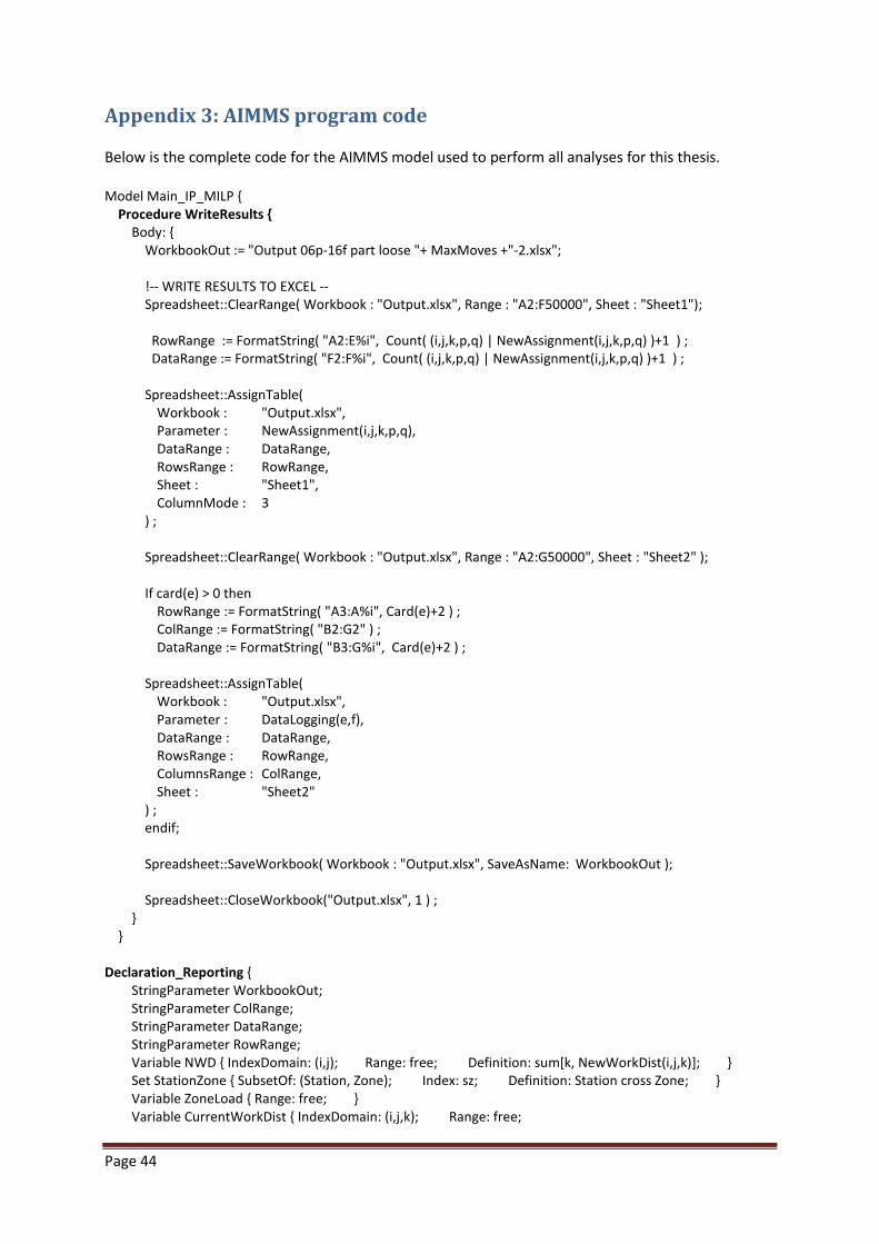
Page 44
Appendix 3: AIMMS program code Below is the complete code for the AIMMS model used to perform all analyses for this thesis. Model Main_IP_MILP { Procedure WriteResults { Body: { WorkbookOut := "Output 06p-16f part loose "+ MaxMoves +"-2.xlsx"; !-- WRITE RESULTS TO EXCEL -- Spreadsheet::ClearRange( Workbook : "Output.xlsx", Range : "A2:F50000", Sheet : "Sheet1"); RowRange := FormatString( "A2:E%i", Count( (i,j,k,p,q) | NewAssignment(i,j,k,p,q) )+1 ) ; DataRange := FormatString( "F2:F%i", Count( (i,j,k,p,q) | NewAssignment(i,j,k,p,q) )+1 ) ; Spreadsheet::AssignTable( Workbook : "Output.xlsx", Parameter : NewAssignment(i,j,k,p,q), DataRange : DataRange, RowsRange : RowRange, Sheet : "Sheet1", ColumnMode : 3 ) ; Spreadsheet::ClearRange( Workbook : "Output.xlsx", Range : "A2:G50000", Sheet : "Sheet2" ); If card(e) > 0 then RowRange := FormatString( "A3:A%i", Card(e)+2 ) ; ColRange := FormatString( "B2:G2" ) ; DataRange := FormatString( "B3:G%i", Card(e)+2 ) ; Spreadsheet::AssignTable( Workbook : "Output.xlsx", Parameter : DataLogging(e,f), DataRange : DataRange, RowsRange : RowRange, ColumnsRange : ColRange, Sheet : "Sheet2" ) ; endif; Spreadsheet::SaveWorkbook( Workbook : "Output.xlsx", SaveAsName: WorkbookOut ); Spreadsheet::CloseWorkbook("Output.xlsx", 1 ) ; } } Declaration_Reporting { StringParameter WorkbookOut; StringParameter ColRange; StringParameter DataRange; StringParameter RowRange; Variable NWD { IndexDomain: (i,j); Range: free; Definition: sum[k, NewWorkDist(i,j,k)]; } Set StationZone { SubsetOf: (Station, Zone); Index: sz; Definition: Station cross Zone; } Variable ZoneLoad { Range: free; } Variable CurrentWorkDist { IndexDomain: (i,j,k); Range: free;

Page 45
Definition: sum [ (p,q), Demand(p,q) * CurrentAssignment(i,j,k,p,q) * LocWeight(k) ]; } Variable NewWorkDist { IndexDomain: (i,j,k); Range: free; Definition: sum [ (p,q), Demand(p,q) * NewAssignment(i,j,k,p,q) * LocWeight(k) ]; } } Declaration_Model_Variables { Parameter StatCount { Range: { {1..6} } } Parameter MinMaxTest { Definition: { Max((i,j), sum[(k,p,q)| Products(p,q) > 0, Demand(p,q) * NewAssignment(i,j,k,p,q) * LocWeight(k) ]) - Min((i,j), sum[(k,p,q)| Products(p,q) > 0, Demand(p,q) * NewAssignment(i,j,k,p,q) * LocWeight(k) ]) } } Set LogCols { SubsetOf: Integers; Index: f; Definition: data { 1 .. 6 }; } Parameter LogCounter { Range: integer; } Set LogRows { SubsetOf: Integers; Index: e; Definition: data { 1 .. 100 }; } Parameter DataLogging { IndexDomain: (e, f); Range: nonnegative; } Parameter IntValues { Range: integer; Definition: sum [ (i,j,k,p,q), NewAssignment(i,j,k,p,q) | NewAssignment(i,j,k,p,q) = 1 ]; } Set PartialVariableSet { SubsetOf: AllVariables; } Set PartialConstraintSet { SubsetOf: AllConstraints; Definition: { data { NWD, CurrentWorkDist, NewWorkDist, Moves, LoadReq, MoveReq, TotMovesReq, SingleAssReq, LocationReq, StationReq, StationReq1 } } } MathematicalProgram LeastDemandVariation { Objective: Workload; Direction: minimize; Constraints: PartialConstraintSet; Variables: AllVariables; Type: Automatic; } Set ZoneStarSet { SubsetOf: Zone; Index: j1; Definition: { {j | j >= ZoneStar} } } Set Station { SubsetOf: Integers; Index: i; } Set Zone { SubsetOf: Integers; Index: j; } Set Rack { SubsetOf: Integers; Index: k; } Set Family { SubsetOf: Integers; Index: p; } Set Sequence { SubsetOf: Integers; Index: q; } ElementParameter ZoneStar { Range: Zone; } Parameter BigM { IndexDomain: p; Definition: sum[q, Products(p,q)]; } Parameter Locations { IndexDomain: (i,j,k); Range: { {0..inf} } } Parameter Demand { IndexDomain: (p,q); Range: nonnegative; } Parameter FamSequence { IndexDomain: p; Range: binary; } Parameter MaxMoves; Parameter LocWeight { IndexDomain: k; } Parameter CurrentAssignment { IndexDomain: (i,j,k,p,q); Range: binary; } Parameter Products { IndexDomain: (p,q); } Variable NewAssignment { IndexDomain: (i,j,k,p,q); Range: [0, 1]; } Variable FamilyAssignment { IndexDomain: (i,p); Range: binary; } Variable MoveTracker { IndexDomain: (i,j,k,p,q) | Products(p,q) > 0; Range: [0, 1]; } Variable Moves { Range: free; Definition: sum[(i,j,k,p,q), MoveTracker(i,j,k,p,q) ]; } Variable Workload { Range: free; } Constraint LoadReq { IndexDomain: (i,j); Definition: { sum[(k,p,q)| Products(p,q) > 0, Demand(p,q) * NewAssignment(i,j,k,p,q) * LocWeight(k) ] <= Workload } } Constraint MoveReq { IndexDomain: (i,j,k,p,q) | Products(p,q) > 0; Definition: CurrentAssignment(i,j,k,p,q) - NewAssignment(i,j,k,p,q) <= MoveTracker(i,j,k,p,q); } Constraint TotMovesReq { Definition: sum[(i,j,k,p,q) | Products(p,q) > 0, MoveTracker(i,j,k,p,q) ] <= MaxMoves; }

Page 46
Constraint SingleAssReq { IndexDomain: (p,q) | Products(p,q) > 0; Definition: sum[(i,j,k), NewAssignment(i,j,k,p,q)] = 1; } Constraint LocationReq { IndexDomain: (i,j,k); Definition: sum[(p,q)| Products(p,q) > 0, NewAssignment(i,j,k,p,q) ] <= Locations(i,j,k); } Constraint StationReq { IndexDomain: (i,p); ActivatingCondition: FamilyAssignment(i,p) = 0; Definition: { !Indicator constraint: sum[(j,k,q)| Products(p,q) > 0, NewAssignment(i,j,k,p,q)] = 0 !Sharp big-M: sum[(j,k,q)| Products(p,q) > 0, NewAssignment(i,j,k,p,q)] <= BigM(p) * FamilyAssignment(i,p) !Loose big-M: sum[(j,k,q)| Products(p,q) > 0, NewAssignment(i,j,k,p,q)] <= 1000 * FamilyAssignment(i,p) } } Constraint StationReq1 { IndexDomain: p; Definition: sum[i, FamilyAssignment(i,p) ] = 1; } Constraint SequenceReq1 { IndexDomain: (p,q) | ord(q) > 1 | Products(p,q) > 0; Definition: { sum[(i,j,k), NewAssignment(i,j,k,p,q) * FamSequence(p)] >= sum[(i,k), NewAssignment(i,first(j),k,p,q-1) * FamSequence(p)] } } Constraint SequenceReq2 { IndexDomain: (p,q) | ord(q) > 1 | Products(p,q) > 0; Definition: { sum[(i,j,k)|ord(j)>1, NewAssignment(i,j,k,p,q) * FamSequence(p)] >= sum[(i,k), NewAssignment(i,nth(j,2),k,p,q-1) * FamSequence(p)] } } Constraint SequenceReq3 { IndexDomain: (p,q) | ord(q) > 1 | Products(p,q) > 0; Definition: { sum[(i,j,k)|ord(j)>2, NewAssignment(i,j,k,p,q) * FamSequence(p)] >= sum[(i,k), NewAssignment(i,nth(j,3),k,p,q-1) * FamSequence(p)] } } Constraint SequenceReq4 { IndexDomain: (p,q) | ord(q) > 1 | Products(p,q) > 0; Definition: { sum[(i,j,k)|ord(j)>3, NewAssignment(i,j,k,p,q) * FamSequence(p)] >= sum[(i,k), NewAssignment(i,nth(j,4),k,p,q-1) * FamSequence(p)] } } Constraint SequenceReq5 { IndexDomain: (p,q) | ord(q) > 1 | Products(p,q) > 0; Definition: { sum[(i,j,k)|ord(j)>4, NewAssignment(i,j,k,p,q) * FamSequence(p)] >= sum[(i,k), NewAssignment(i,nth(j,5),k,p,q-1) * FamSequence(p)] } } Constraint SequenceReq6 { IndexDomain: (p,q) | ord(q) > 1 | Products(p,q) > 0; Definition: { sum[(i,k), NewAssignment(i,last(j),k,p,q) * FamSequence(p)] >= sum[(i,k), NewAssignment(i,last(j),k,p,q-1) * FamSequence(p)] } } } Procedure MainInitialization { Body: { Family := DATA { 1 .. 56 } ; Sequence := DATA { 1 .. 65 } ; read from file "Data input reduced.txt" ; Spreadsheet::RetrieveTable( workbook : WorkbookName, Parameter : CurrentAssignment(i,j,k,p,q), DataRange : "F2:F2649", RowsRange : "A2:E2649", Sheet : "Assignment" ); Spreadsheet::RetrieveTable( workbook : WorkbookName, Parameter : Locations(i,j,k), DataRange : "I2:J37", RowsRange : "G2:H37", ColumnsRange : "I1:J1", Sheet : "Locations" ); Spreadsheet::RetrieveTable(

Page 47
workbook : WorkbookName, Parameter : Demand(p,q), DataRange : "C2:C2649", RowsRange : "A2:B2649", Sheet : "Demand" ); Spreadsheet::RetrieveTable( workbook : WorkbookName, Parameter : Products(p,q), DataRange : "B2:BN57", RowsRange : "A2:A57", ColumnsRange : "B1:BN1", Sheet : "Product" ); Spreadsheet::RetrieveTable( workbook : WorkbookName, Parameter : FamilyAssignment(i,p), DataRange : "G2:BJ7", RowsRange : "F2:F7", ColumnsRange : "G1:BJ1", Sheet : "Family" ); Spreadsheet::CloseWorkbook(WorkbookName, 1 ) ; } } Declaration_Data_Input { DatabaseTable KnappData { DataSource: "KnappDWH"; } StringParameter WorkbookName { InitialData: "Input data validation.xlsx"; } } Procedure MainExecution { Body: { MaxMoves := 10; While (MaxMoves <= 160) do ! Validation assignment as start assignment !Spreadsheet::RetrieveTable( ! workbook : WorkbookName, ! Parameter : FamilyAssignment(i,p), ! DataRange : "G2:BJ7", ! RowsRange : "F2:F7", ! ColumnsRange : "G1:BJ1", ! Sheet : "Family" !); !Spreadsheet::CloseWorkbook(WorkbookName, 1 ) ; ! Generated assignment as start assignment FamilyAssignment(i,p) := 0; StatCount := 1; for (p) do FamilyAssignment(StatCount, p) := 1; if StatCount < 6 then StatCount += 1;

Page 48
else StatCount := 1; endif; endfor; NewAssignment(i,j,k,p,q) := CurrentAssignment(i,j,k,p,q) ; MoveTracker(i,j,k,p,q) := 0 ; Moves := 0 ; Workload := 0 ; DataLogging(e, f) := 0; LogCounter := 1; LeastDemandVariation.CallbackNewIncumbent := 'NewIncumbent'; solve LeastDemandVariation ; DataLogging(LogCounter, 1) := LeastDemandVariation.nodes ; DataLogging(LogCounter, 2) := LeastDemandVariation.SolutionTime; DataLogging(LogCounter, 3) := LeastDemandVariation.LinearObjective ; DataLogging(LogCounter, 4) := LeastDemandVariation.Incumbent ; DataLogging(LogCounter, 5) := LeastDemandVariation.Objective ; DataLogging(LogCounter, 6) := IntValues ; WriteResults; MaxMoves += 10; endwhile; } } Procedure NewIncumbent { Body: { RetrieveCurrentVariableValues(AllVariables); DataLogging(LogCounter, 1) := LeastDemandVariation.nodes ; DataLogging(LogCounter, 2) := LeastDemandVariation.SolutionTime; DataLogging(LogCounter, 3) := LeastDemandVariation.LinearObjective ; DataLogging(LogCounter, 4) := LeastDemandVariation.Incumbent ; DataLogging(LogCounter, 5) := LeastDemandVariation.Objective ; DataLogging(LogCounter, 6) := IntValues ; LogCounter += 1; Return 1; } } Declaration_Execution { Parameter BestBound; ElementParameter MasterProblem_GMP { Range: AllGeneratedMathematicalPrograms; } } Procedure MainTermination { Body: { return DataManagementExit(); } } }

Page 49
Bibliography The following literature has been used in this thesis. The references are ordered in alphabetical order by author. Aboudi, R. and K. Jørnsten (1990). "Resource constrained assignment problems." Discrete applied mathematics
26(2): 175-191.
Aggarwal, V., et al. (1986). "Bottleneck assignment problems under categorization." Computers & Operations Research
13(1): 11-26.
AIMMS (2015). Retrieved 30 May, 2015, from http://www.aimms.com/aimms/solvers/cplex/. Aneja, Y. P. and A. P. Punnen (1999). "Multiple bottleneck assignment problem." European Journal of Operational Research
112(1): 167-173.
Bauer, U. (2005). Assignment Problem with Constraints. Faculty of Informatics
. Munchen, TU Munchen.
Berkelaar, M., et al. (2015, April 10th, 2015). Retrieved June 6th, 2015, from http://lpsolve.sourceforge.net/. Bertsekas, D. P., et al. (1993). "Reverse auction and the solution of inequality constrained assignment problems." SIAM Journal on Optimization
3(2): 268-297.
Bixby, R. E. (1992). "Implementing the simplex method: The initial basis." ORSA Journal on Computing
4(3): 267-284.
Burkard, R. E., et al. (2009). Assignment Problems, Revised Reprint
, Siam.
Camm, J. D., et al. (1990). "Cutting big M down to size." Interfaces
20(5): 61-66.
Caron, G., et al. (1999). "The assignment problem with seniority and job priority constraints." Operations research
47(3): 449-453.
De Koster, R. (2004). "How to assess a warehouse operation in a single tour." Technology Report. RSM Erasmus Unversity, the Netherlands
.
De Koster, R., et al. (2007). "Design and control of warehouse order picking: A literature review." European Journal of Operational Research
182(2): 481-501.
De Koster, R. and M. Yu (2008). "Minimizing makespan and throughput times at Aalsmeer flower auction." Journal of the Operational Research Society
59(9): 1182-1190.
Dell'Amico, M. and P. Toth (2000). "Algorithms and codes for dense assignment problems: the state of the art." Discrete applied mathematics
100(1): 17-48.
Duin, C. and A. Volgenant (1991). "Minimum deviation and balanced optimization: A unified approach." Operations Research Letters
10(1): 43-48.
Ford, L. and D. Fulkerson (1962). Flows in networks, Princeton Princeton University Press.

Page 50
Frazelle, E. and G. Sharp (1989). Correlated assignment strategy can improve order-picking operation. Industrial Engineering
: 5.
Garey, M. R. and D. S. Johnson (1979). "Computer and intractability." A Guide to the Theory of NP-Completeness
.
Heskett, J. L. (1963). "Cube-per-order index-a key to warehouse stock location." Transportation and distribution Management
3(1): 27-31.
IBM (2005, 20 December 2005). "CPLEX Performance Tuning for Mixed Integer Programs." FAQ. Retrieved 22 May, 2015, from http://www-01.ibm.com/support/docview.wss?uid=swg21400023. Jane, C. C. (2000). "Storage location assignment in a distribution center." International Journal of Physical Distribution & Logistics Management
30(1): 55-71.
Kennington, J. and Z. Wang (1992). "A shortest augmenting path algorithm for the semi-assignment problem." Operations research
40(1): 178-187.
Kofler, M., et al. (2014). Affinity Based Slotting in Warehouses with Dynamic Order Patterns. Advanced Methods and Applications in Computational Intelligence
, Springer: 123-143.
Kofler, M., et al. (2011). Re-warehousing vs. healing: Strategies for warehouse storage location assignment
. Logistics and Industrial Informatics (LINDI), 2011 3rd IEEE International Symposium on, IEEE.
Koo, P.-H. (2009). "The use of bucket brigades in zone order picking systems." OR spectrum
31(4): 759-774.
Kuhn, H. W. (1955). "The Hungarian method for the assignment problem." Naval research logistics quarterly
2(1-2): 83-97.
Makhorin, A. O. (2015, June 23rd, 2012). Retrieved June 6th, 2015, 2015, from http://www.gnu.org/software/glpk/. Malmborg, C. J. (1995). "Optimization of cube-per-order index warehouse layouts with zoning constraints." THE INTERNATIONAL JOURNAL OF PRODUCTION RESEARCH
33(2): 465-482.
Martello, S., et al. (1984). "Balanced optimization problems." Operations Research Letters
3(5): 275-278.
Mazzola, J. B. and A. W. Neebe (1986). "Resource-constrained assignment scheduling." Operations research
34(4): 560-572.
Murty, K. G. (1994). Operations research: deterministic optimization models
, Prentice-Hall, Inc.
Papadimitriou, C. H. and K. Steiglitz (1998). Combinatorial optimization: algorithms and complexity
, Courier Dover Publications.
Pentico, D. W. (2007). "Assignment problems: A golden anniversary survey." European Journal of Operational Research
176(2): 774-793.

Page 51
Petersen II, C. G. (1997). "An evaluation of order picking routeing policies." International Journal of Operations & Production Management
17(11): 1098-1111.
Punnen, A. and Y. Aneja (1993). "Categorized assignment scheduling: A tabu search approach." Journal of the Operational Research Society
: 673-679.
Punnen, A. P. (2004). "On bottleneck assignment problems under categorization." Computers & Operations Research
31(1): 151-154.
Rardin, R. L. (1998). Optimization in operations research
, Prentice Hall New Jersey.
Richards, A. and J. How (2005). Mixed-integer programming for control
. American Control Conference, 2005. Proceedings of the 2005, IEEE.
Roelofs, M. and J. Bisschop (2014). "AIMMS: The Language Reference." Paragon Decision Technology
.
Tolliver, R. (1989). "Order picking basics at avon products." Material Handling Focus
89.
Tompkins, J., et al. (2003). Facilities Planning, NJ: John Wiley & Sons. Unterhofer, W. (2003). Effiziente Berechnung von minimalen perfekten Matchings in gewichteten bipartiten Graphen. Faculty of Informatics
. Munchen, TU Munchen.
Valeant (2015). "Key Facts & History." Retrieved 1/3/2015, 2015, from www.valeant.com/about/key-facts. Volgenant, A. (1996). "Linear and semi-assignment problems: a core oriented approach." Computers & Operations Research
23(10): 917-932.
Volgenant, A. (2004). "A note on the assignment problem with seniority and job priority constraints." European Journal of Operational Research
154(1): 330-335.
Yu, M. and R. De Koster (2008). "Performance approximation and design of pick-and-pass order picking systems." IIE Transactions
40(11): 1054-1069.