application note an 20-001 module temperature sensor

© by SEMIKRON / 2020-01-29 / Application Note PROMGT.1023/ Rev.7/ Template Application Note

/22

Calculating Junction Temperature using a Module Temperature Sensor1. Introduction .............................................................................................................................1

2. Temperature Prediction Goals .....................................................................................................22.1 Over temperature protection .................................................................................................22.2 Performance optimization......................................................................................................22.3 Lifetime prediction ...............................................................................................................2

3. Integrated Temperature Sensors .................................................................................................33.1 Why are no Rth(j-r)/Zth(j-r) values specified in the module data sheet?............................................3

3.1.1 Influence of heatsink ......................................................................................................33.1.2 Influence of operating point.............................................................................................4

4. Determining Rth(j-r)/Zth(j-r)............................................................................................................64.1 Measurement methods..........................................................................................................6

4.1.1 Thermocouple (Rth) ........................................................................................................74.1.2 Infrared camera (Rth) .....................................................................................................84.1.3 Vce method (Rth or Zth) ....................................................................................................94.1.4 Finite Element Analysis (Rth or Zth) ...................................................................................9

5. Simplified Method for Periodic Functions (Quasi-Steady State Conditions) .......................................105.1 Required circuit parameters (inverter example) ......................................................................105.2 Loss calculation..................................................................................................................105.3 Junction temperature calculation ..........................................................................................115.4 Correction factor for low output frequencies ...........................................................................125.5 Example (Three-phase PWM inverter) ...................................................................................13

6. Thermal Coupling ....................................................................................................................146.1.1 Determination of Rth/Zth matrix ......................................................................................16

7. Complex Method, Step-by-Step (Short, High Overload and Stall Torque Conditions) .........................177.1 Required circuit parameters (inverter example) ......................................................................177.2 Loss calculation..................................................................................................................177.3 Junction temperature calculation ..........................................................................................187.4 Example............................................................................................................................19

8. Summary ...............................................................................................................................20

1. Introduction

A legitimate but complex question is how does one use the integrated temperature sensor inside a power semiconductor module to determine the virtual junction temperature? There are several answers depending on the required accuracy and the goal of the temperature prediction. This application note will explain two possible methods: one at the lower end and one at the higher end of the complexity scale. It is first necessary

Application NoteAN 20-001

Revision: 02 Issue date: 2020-01-29Prepared by: P. Drexhage, A. Wintrich Approved by: P. Beckedahl

Keyword: IGBT module, temperature sensor, thermal impedance


/22

to define the goals of the temperature prediction because it has an impact on the required device parameters, qualification effort, and computing power for calculation. This document uses the example of a three-phase 2-level inverter circuit with IGBT and freewheeling diodes but these methods can be applied to other circuits and semiconductors as well. Though the proposed procedures refer to module-integrated temperature sensors, they can also be used for external sensors (e.g. on the heatsink). The intention is that the calculation methods are implemented using a digital processor on a converter control board.

Table 1: Comparison of the two considered methods for junction temperature prediction

Simplified solution for quasi-steady state conditions

Complex solution for short high overload and stall torque conditions

Calculation of losses in one switch and assuming that the other switches in a symmetric circuit have equal losses (e.g. IGBT1…6 in a three-phase inverter)

Calculation of the losses for any switch according to actual circuit conditions (VCC, Vout, Iout, cos(φ), fsw, Tj)

Only one thermal model (Tj to sensor Tr) per type of switch is required (e.g. one for diode, one for IGBT)

Calculation of the junction temperature using a Zth(j-

r)-matrix including coupling of all relevant switches

Sampling rates on the order of 100ms…1s which allows use of Rth instead of Zth

Sampling rate on the order of 1/fsw (or multiples of that)

Result: average losses of periodic function and average junction temperatures

Result: instantaneous function of losses and device temperatures

Correction factor used to account for temperature ripple due to fundamental output frequency

Temperature swing with inverter output frequency is inherently calculated

“Envelope curve” for temperatures usable for device protection

Advantage: Low computing power and data volume

Advantages: Protection at low frequency or stall torque possible. Information about temperature cycle stress available.

Disadvantages: Limited protection in stall torque or at short high overload. No usable information for temperature cycle stress calculations.

Disadvantages: High effort for model implementation. High computing power required. High data volume.

2. Temperature Prediction Goals

2.1 Over temperature protectionThe most common use of temperature monitoring is simply to protect the semiconductors from operating above their thermal limits. With gradually increasing junction temperature situations (e.g. increases in ambient temperature or low magnitude/long duration overloads), this can be accomplished by comparing the sensor temperature with a pre-determined (at the design stage) set point at which the system faults (or issues a warning). For dynamic loads, power fold back curves can be developed which maximize the output current at a given temperature (e.g. high current at low ambient temperature).

2.2 Performance optimizationThe maximum output power of a system at a given operating point can depend on a variety of factors, among them environmental (ambient air temperature, altitude) as well as electrical (fundamental output frequency). The output current can be maximized for a given operating point while ensuring that the junction temperature does not exceed its limits. However, this approach carries the risk of reducing power module lifetime if the additional temperature stress is not considered (see explanation of power cycling in [2]).

2.3 Lifetime predictionMost power cycling lifetime models are based primarily on the mean junction temperature and number of junction temperature excursions (sec. 2.7.6 in [2]). In theory, this means that a system that is able to calculate and store the value of actual junction temperature during operation could actively apply a lifetime


/22

model to determine the “life remaining” in a system. In practice, this has proven difficult to achieve due to the uncertainty of lifetime models coupled with the complexity (and cost) of storing, processing, and evaluating such data in the field.

3. Integrated Temperature Sensors

Modern power semiconductor modules incorporate a temperature-sensitive resistive element (thermistor; NTC or PTC) soldered on the DBC substrate. Due to layout restrictions (e.g. voltage isolation), the temperature (Tr) of this sensor does not represent the actual IGBT or diode junction temperature.

Figure 1: Location of temperature sensors in baseplate-less MiniSKiiP (L) and baseplate-d SEMiX3p (R)

For SEMIKRON product, the temperature of the sensor may be specified as approximating an existing reference point (e.g. Tc or Ts). This is specified in the Technical Explanations for the product. For example:

SEMiX3s: Sensor is on a separate DBC substrate Tr is close to Ts SKiiP4: Sensor is on the same copper trace as IGBT and diode Ts < Tr < Tj

However, this simplification should be used with caution as Tr can vary depending on a number of conditions. In some cases, the sensor temperature may be lower than the heatsink temperature beneath the hottest chip.

The temperature sensor can be treated as a node within a simplified Foster thermal network. If only overtemperature protection for slowly changing loads is required and the sensor temperature is equal to heatsink temperature, then the datasheet values for Rth(j-s) can be used with safety margin to estimate junction temperature. For more accurate results under dynamic conditions, a dedicated Zth(j-r) must be determined.

3.1 Why are no Rth(j-r)/Zth(j-r) values specified in the module data sheet?The sensor temperature and resulting thermal impedance from “junction to sensor” depend on many conditions that are outside the design of the module itself. These conditions influence both lateral temperature spreading and vertical heat conductivity in the system and can be divided roughly into two parts.

3.1.1 Influence of heatsinkThe mechanical design of the heatsink influences the distribution of heat beneath the module, due in part to:

Cooling medium (air or liquid) Material and root thickness of the heatsink Conductivity and thickness of thermal paste layer Module and sensor position on heatsink (distance to edges and flow direction of cooling medium, see

Figure 2) Distance to other modules on the same heatsink


/22

Figure 2: Effect of module mounting position on sensor temperature

Therefore, power semiconductor modules are specified in their data sheet with Rth(j-s) or Rth(j-c) and not Rth(j-

r), except for modules that are qualified and delivered together with a heatsink (SKiiP).

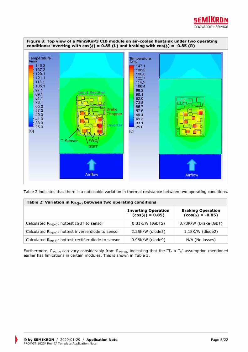
3.1.2 Influence of operating pointThe electrical operating point of the system determines the magnitude and distribution of losses between switches within the module.

Figure 3 shows two simulations of a 50A/1200V Converter-Inverter-Brake (CIB) module on an air cooled heatsink (Ta = 25°C, Rth(s-a) ≈ 0.13K/W). The left side shows the condition of “inverter” operation (22kW, cos() = 0.85) with high load on the IGBT and the DC-link fed by the input rectifier. The right side shows the same module during “brake” operation (22kW, cos() = -0.85) with the braking energy dissipated by the brake chopper. The temperature sensor is at the lower left corner.

Tj=142°C

Airflow

Tr=102°C

Tr=92°CTj=142°C

Airflow


/22

Figure 3: Top view of a MiniSKiiP3 CIB module on air-cooled heatsink under two operating conditions: inverting with cos() = 0.85 (L) and braking with cos() = -0.85 (R)

FWDIGBT

Input Rectifier

Brake Chopper

T-Sensor

Inverter1

54

62

3

Airflow

Table 2 indicates that there is a noticeable variation in thermal resistance between two operating conditions.

Table 2: Variation in Rth(j-r) between two operating conditions

Inverting Operation(cos() = 0.85)

Braking Operation(cos() = -0.85)

Calculated Rth(j-r): hottest IGBT to sensor 0.81K/W (IGBT5) 0.73K/W (Brake IGBT)

Calculated Rth(j-r): hottest inverse diode to sensor 2.25K/W (diode5) 1.18K/W (diode2)

Calculated Rth(j-r): hottest rectifier diode to sensor 0.96K/W (diode9) N/A (No losses)

Furthermore, Rth(j-r) can vary considerably from Rth(j-s), indicating that the “Tr ≈ Ts” assumption mentioned earlier has limitations in certain modules. This is shown in Table 3.

Airflow


/22

Table 3: Effect of “Ts = Tr” assumption on calculated temperatures

Inverting Operation(cos() = 0.85)

IGBT: 60WInverse diode: 12WRectifier diode: 20W

Rth(j-r): hottest IGBT to sensor 0.81K/W (IGBT5)

ΔTj-r_IGBT 60W * 0.81K/W = 48.6K

Datasheet Rth(j-s)_IGBT 0.71K/W

Calculated ΔTj-r (assumption: Tr ≈ Ts) 60W * 0.71K/W = 42.6K (6K too low)

Calculated Rth(j-r): hottest inverse diode to sensor 2.25K/W (diode5)

ΔTj-r_inverse_diode 12W * 2.25K/W = 27K

Datasheet Rth(j-s)_diode 0.95K/W

Calculated ΔTj-r (assumption: Tr ≈ Ts) 12W * 0.95K/W = 11.4K (15.6K too low)

Calculated Rth(j-r): hottest rectifier diode to sensor 0.96K/W (diode9)

ΔTj-r_rectifier 20W * 0.96K/W = 19.2K

Datasheet Rth(j-s)_rectifier 0.9K/W

Calculated ΔTj-r (assumption: Tr ≈ Ts) 20W * 0.9K/W = 18K (1.2K too low)

4. Determining Rth(j-r)/Zth(j-r)

4.1 Measurement methodsFor the reasons listed above, the thermal resistance/impedance from junction to sink must be determined for each application. Three experimental methods can be used to determine the thermal resistance between each individual IGBT or diode switch and the thermal sensor. These results should then be compared with a computer-based finite element model to verify the tests and allow for quicker derivation of thermal resistance under other operating conditions.

In each test, a current is fed through a single switch and the temperatures of the sensor and a target switch are measured (Figure 4).

For Rth(j-r), the current is a fixed direct current and the temperature of the sensor measured once stabilized. For Zth(j-r), the current is a step function and the temperature is sensor measured continuously. The current and the voltage across the switch are used to calculate the losses. In practice a step down function is used (turn-off power dissipation) and the measured temperatures are inverted later as this is the only way to reach steady state for temperature dependent losses.


/22

Figure 4: Application of current and resulting temperatures

Switch(BOT IGBT)

Iload(Step)

+-15V

Vdevice

Pdevice = Iload · Vdevice0

20

40

60

80

100

120

140

160

0,001 0,01 0,1 1 10 100 1000

T [°

C]

t [s]

Phase U TOP IGBT

Tj [°C]

Tr [°C]

dT(j-r) [K]

Iload

Transient(to calculate Zth)

Steady-state(to calculate Rth)

4.1.1 Thermocouple (Rth)A specially prepared module is obtained from the manufacturer where thermocouples have been glued to the surface of the chips with thermally conductive epoxy (Figure 5). A regulated direct current (at low voltage) is put through the IGBT or diode and the temperature of the thermocouple and temperature sensor are measured to calculate the temperature difference.

(1)Rth(j ‒ r) =Tj_device_thermocouple ‒ Tr

Pdevice

Due to the slow time response of thermocouples, only determination of static thermal resistance Rth(j-r) is possible. Furthermore, the thermocouples themselves can introduce 5…15°C of error as the metal wire acts as a heatsink on the top surface of the chip. Caution must be taken to isolate the thermocouples where they connect with measurement equipment.


/22

Figure 5: SEMiX3p module with thermocouples added to the IGBT chips

Tr = internal NTC sensor

Tj_IGBT4 Tj_IGBT3 Tj_IGBT2 Tj_IGBT1

4.1.2 Infrared camera (Rth)A specially prepared module without silicone soft mould is used. The housing cover is removed and the interior of the module coated with a matte paint with uniform emissivity to prevent reflections. A regulated direct current (at low voltage) is put through the IGBT or diode and the temperature reported by the camera and the temperature sensor are measured to calculate the temperature difference (Figure 6).

(2)Rth(j ‒ r) =Tj_device_IR_camera ‒ Tr

Pdevice

If properly calibrated a high resolution infrared camera gives accurate temperatures although at a slow enough refresh rate that only determination of static thermal resistance Rth(j-r) is possible. Furthermore, modules with internal busbars system cannot be easily measured as the view of the chips is blocked.


/22

Figure 6: SEMiX3p module under infrared imaging

4.1.3 Vce method (Rth or Zth)Semiconductors have a linear relationship between junction temperature, Tj, and forward voltage drop, Vce/Vf, at low currents. Using uniform heating in a lab environment, a calibration curve for a particular semiconductor type can be derived (Figure 7). The module is then placed in a fixture where a high current pulse is put through the semiconductor to generate losses and is followed quickly by a low current to measure the forward voltage drop (and hence the junction temperature.)

Figure 7: Test configuration and example calibration curve

050

100150200250300350400450500

20 40 60 80 100 120Tj [°C]

VCE

0 [m

V]

This method provides highly accurate results and can be used to determine the transient thermal impedance (Zth) of the junction-to-sensor interface. However, it usually requires purpose-built test equipment.

4.1.4 Finite Element Analysis (Rth or Zth)Finite Element Analysis (FEA) is achieved by modelling the module-heatsink system in software. In order to construct this model, two items are required from the module manufacturer:

The X-Y locations of the chips within the module (“die map,” “chip layout”). The thickness, density, thermal conductivity, and thermal capacity of the layers making up the

module in the Z-axis (“material stack-up”).


/22

Once the model is constructed, losses can be applied to each switch and the junction, heatsink, and sensor temperatures determined. This method should be done in conjunction with one of the other test methods to verify the accuracy of the model (and vice versa).

5. Simplified Method for Periodic Functions (Quasi-Steady State Conditions)

An integral solution calculates average losses of the devices over a period (e.g. one fundamental cycle for a PWM inverter). The device losses are the sum of conduction losses, Pcond, and switching losses, Psw. The sampling rate is low, for example, in the range of 10/fout up to 1s. Therefore, a static thermal resistance, Rth(j-r), is used. The losses are temperature-dependent which means an iterative calculation with Tj as an additional input is required. If the losses do not change too much from time step to time step then Tj from the previous time step can be used.

5.1 Required circuit parameters (inverter example)Irms - Fundamental output current, RMSM - Modulation depthcos(φ) - Power factorVcc - DC link voltagefsw - Switching (carrier) frequencyfout - Fundamental output frequency

5.2 Loss calculationCycle average losses for an IGBT in a three-phase PWM inverter:

Pcond_IGBT = ( 12π +

M ∙ cos(φ)8 ) ∙ (VCE0_25°C + TCVce ∙ (Tj - 25°C)) ∙ Ipk + (1

8 +M ∙ cos(φ)

3π ) ∙ (rCE_25°C + TCrce ∙ (Tj - 25°C)) ∙

(3)Ipk2

(4)Psw_IGBT = fsw ∙ Eon + off ∙1

2π ∙ (Ipk

Iref)Ki

∙ (Vcc

Vref)Kv

∙ (1 + TCsw ∙ (Tj - Tjref)) ∙ γ(Ki)

Cycle average losses for a diode in a three-phase PWM inverter:

Pcond_D = ( 12π ‒

M ∙ cos(φ)8 ) ∙ (VF0_25°C + TCVf ∙ (Tj - 25°C)) ∙ Ipk + (1

8 ‒M ∙ cos(φ)

3π ) ∙ (rf_25°C + TCrf ∙ (Tj - 25°C)) ∙ Ipk2

(5)

(6)Psw_D = fsw ∙ Err ∙1

2π ∙ (Ipk

Iref)Ki

∙ (Vcc

Vref)Kv

∙ (1 + TCsw(Tj - Tjref)) ∙ γ(Ki)

Ki - Exponent of current dependency (IGBT ≈ 1, FWD ≈ 0.6)Kv - Exponent of voltage dependency (IGBT ≈ 1.35, FWD ≈ 0.6)TCsw - Temperature coefficient (IGBT ≈ 0.003, FWD ≈ 0.006)

γ(Ki) - Integral (IGBT: γ(1) = 2, FWD: γ(0.6) = 2.3)∫π + φφ sin

Ki(α - φ)dα

Where the following are given in the module datasheet:

VCE0_25°CrCE_25°CEon+off (measured at Iref, Vref, Tjref)TCVce (calculated as a linear relationship between VCE0(low temp) and VCE0(high temp))TCrce (calculated as a linear relationship between rCE(low temp) and rCE(high temp))

VF0_25°CRF_25°C


/22

Err (measured at Iref, Vref, Tjref)TCVf (calculated as a linear relationship between VF0(low temp) and VF0(high temp))TCrf (calculated as a linear relationship between rf(low temp) and rf(high temp))

See also [2].

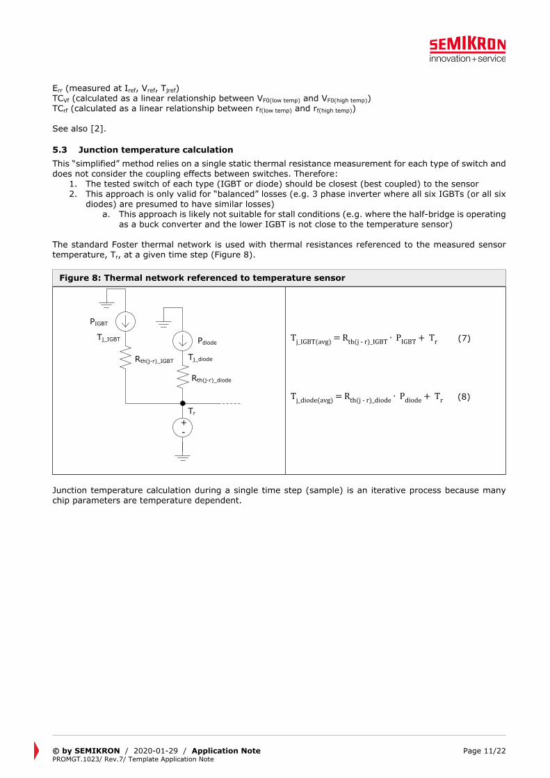
5.3 Junction temperature calculationThis “simplified” method relies on a single static thermal resistance measurement for each type of switch and does not consider the coupling effects between switches. Therefore:

1. The tested switch of each type (IGBT or diode) should be closest (best coupled) to the sensor2. This approach is only valid for “balanced” losses (e.g. 3 phase inverter where all six IGBTs (or all six

diodes) are presumed to have similar losses)a. This approach is likely not suitable for stall conditions (e.g. where the half-bridge is operating

as a buck converter and the lower IGBT is not close to the temperature sensor)

The standard Foster thermal network is used with thermal resistances referenced to the measured sensor temperature, Tr, at a given time step (Figure 8).

Figure 8: Thermal network referenced to temperature sensor

Rth(j-r)_IGBT

Rth(j-r)_diode

Tj_IGBT

Tj_diode

PIGBT

Pdiode

Tr

+-

(7)Tj_IGBT(avg) = Rth(j - r)_IGBT ∙ PIGBT + Tr

(8)Tj_diode(avg) = Rth(j - r)_diode ∙ Pdiode + Tr

Junction temperature calculation during a single time step (sample) is an iterative process because many chip parameters are temperature dependent.


/22

Figure 9: Calculation process during a single time step

Output Tj

Tj[Tj(k)] ≈ Tj(k)?

Set initial Tj(k) = Tr

Calculate device lossesPdevice[Tj(k)] = Pcond[Tj(k)] + Psw[Tj(k)]

Calculate junction temperaturesTj[Tj(k)] = Pdevice[Tj(k)] • Rth(j-r) + Tr

Sample circuit parameters and sensor temperature

Y

N

Adjust Tj for fundamental frequency Tj(max)

Next time step

k = k + 1

5.4 Correction factor for low output frequenciesThe method above yields an average junction temperature and does not indicate the peak temperatures that occur as the junction temperature oscillates at the fundamental output frequency. This is mainly of concern at low (<10Hz) frequency operation. A simple correction factor (as shown in Figure 10) is used to adjust the calculated average temperature. The correction factor depends on the thermal impedance of the devices in use.


/22

Figure 10: Correction factor for Tj(max) = f(fout)

0

0,5

1

1,5

2

2,5

3

0 20 40 60 80 100

F corr

fout [Hz]

Frequency correction factor SKAI-HV

IGBT

Diode

Therefore, the maximum junction temperature during a fundamental cycle can be estimated as:

(9)Tj_IGBT(max) = Fcorr_IGBT ∙ Rth(j - r)_IGBT ∙ PIGBT + Tr

(10)Tj_diode(max) = Fcorr_diode ∙ Rth(j - r)_diode ∙ Pdiode + Tr

5.5 Example (Three-phase PWM inverter)Device parameters from SKiiP39AC12T4V1 datasheet:IGBT: VCE0_25°C=0.8V, rce_25°C=7mΩ, Esw=36.5mJ, TCVce = -0.0008V/K, TCrce = 2.67E-5Ω/KDiode: VF0_25°C=1.3V, rf_25°C=5.6mΩ, Err=11.4mJ, TCVf = -0.0032V/K, TCrf = 1.76E-5Ω/K

Measured Rth(j-r) from testing:Rth(j-r)I = 0.3 K/WRth(j-r)D =0.6 K/W

Initial time step: measured values during operationIout = 76Arms = 107.48ApkM = 1cos(φ) = 0.85VCC = 650Vfsw = 4kHzfout = 20HzTr = 100°C

Calculated losses(First iteration shown)Pcond_IGBT

= ( 12π +

1 ∙ 0.858 ) ∙ (0.8V ‒ 0.0008V/K ∙ (100°C ‒ 25°C)) ∙ 107.48A + (1

8 +1 ∙ 0.85

3π )∙ (0.007Ω + 0.0000267Ω/K ∙ (100°C ‒ 25°C)) ∙ 107.48A2 = 43.49W

Psw_IGBT = 4000Hz ∙ 0.0365J ∙1

2π ∙ (107.48A150A )1

∙ (650V600V)1.35

∙ (1 + 0.003 ∙ (100°C ‒ 150°C)) ∙ 2 = 31.53W


/22

Pcond_D

= ( 12π ‒

1 ∙ 0.858 ) ∙ (1.3V ‒ 0.0032V/K ∙ (100°C ‒ 25°C)) ∙ 107.48A + (1

8 ‒1 ∙ 0.85

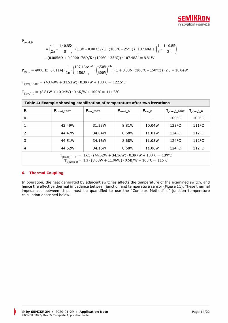
3π )∙ (0.0056Ω + 0.0000176Ω/K ∙ (100°C ‒ 25°C)) ∙ 107.48A2 = 8.81W

Psw_D = 4000Hz ∙ 0.0114J ∙1

2π ∙ (107.48A150A )0.6

∙ (650V600V)0.6

∙ (1 + 0.006 ∙ (100°C ‒ 150°C)) ∙ 2.3 = 10.04W

Tj(avg)_IGBT = (43.49W + 31.53W) ∙ 0.3K/W + 100°C = 122.5°C

Tj(avg)_D = (8.81W + 10.04W) ∙ 0.6K/W + 100°C = 111.3°C

Table 4: Example showing stabilization of temperature after two iterations

K Pcond_IGBT Psw_IGBT Pcond_D Psw_D Tj(avg)_IGBT Tj(avg)_D

0 - - - - 100°C 100°C

1 43.49W 31.53W 8.81W 10.04W 123°C 111°C

2 44.47W 34.04W 8.68W 11.01W 124°C 112°C

3 44.51W 34.16W 8.68W 11.05W 124°C 112°C

4 44.52W 34.16W 8.68W 11.06W 124°C 112°C

Tj(max)_IGBT = 1.65 ∙ (44.52W + 34.16W) ∙ 0.3K/W + 100°C = 139°CTj(max)_D = 1.3 ∙ (8.68W + 11.06W) ∙ 0.6K/W + 100°C = 115°C

6. Thermal Coupling

In operation, the heat generated by adjacent switches affects the temperature of the examined switch, and hence the effective thermal impedance between junction and temperature sensor (Figure 11). These thermal impedances between chips must be quantified to use the “Complex Method” of junction temperature calculation described below.


/22

Figure 11: FEA model of half-bridge module illustrating thermal coupling between chips and temperature sensor

Temp. sensor

TOP BOT

I I

II

I I

I I

D D

D D

The relationship between any one switch and the temperature sensor is thus defined by the effect the losses in the other switches have on the switch in question (Figure 12). The switch for which you are trying to determine the ultimate junction temperature in the application is referred to as the “Self” switch. Note that in this document the definition of “switch” pertains to a single electrical element (e.g. IGBT or diode) as opposed to other documents that refer to a single switch as being composed of an IGBT and diode.


/22

Figure 12: Definition of static coupling for one switch in a hypothetical half-bridge

Switch2(BOT IGBT)

Switch3(TOP diode)

Switch1(TOP IGBT)

PSwitch1(TOP IGBT)

Rth(j-r)_Self

PSwitch2(BOT IGBT)

Rth(j-r)_Switch2

+-

Tj_Switch1

ΔTj-r

PSwitch3(TOP diode)

Rth(j-r)_Switch3

PSwitch4(BOT diode)

Rth(j-r)_Switch4

Tr

Switch4(BOT diode)

Tj_Switch1 = Tr + PSwitch1 ∙ Rth(j ‒ r)_Self + PSwitch2 ∙ Rth(j ‒ r)_Switch2 + PSwitch3 ∙ Rth(j ‒ r)_Switch3 + PSwitch4 ∙(11)Rth(j ‒ r)_Switch4

6.1.1 Determination of Rth/Zth matrixIn a lab setting, losses must be applied to each switch individually and the junction temperature measured using one of the methods in section 4.1. The following example uses the half-bridge circuit from Figure 12.

A. Apply target losses to Switch1 (Self) only. Measure Tj_Switch1 and Tr.Calculate:

(12)Rth(j ‒ r)_Self =Tj_Switch1_A ‒ Tr_A

PSwitch1

B. Apply target losses to Switch2 only. Measure Tj_Switch1 and Tr.Calculate:

(13)Rth(j ‒ r)_Switch2 =Tj_Switch1_B ‒ Tr_B

PSwitch2

C. Apply target losses to Switch3 only. Measure Tj_Switch1 and Tr.Calculate:


/22

(14)Rth(j ‒ r)_Switch3 =Tj_Switch1_C ‒ Tr_C

PSwitch3

D. Apply target losses to Switch4 only. Measure Tj_Switch1 and Tr.Calculate:

(15)Rth(j ‒ r)_Switch4 =Tj_Switch1_D ‒ Tr_D

PSwitch4

Repeat steps A through D for the remaining three switches. The resulting values can be placed in a matrix as shown in Table 5.

Table 5: Rth matrix for hypothetical half-bridge

Apply losses at:

Measure Tj at:

TOP IGBT(Switch1)

BOT IGBT(Switch2)

TOP Diode(Switch3)

BOT Diode(Switch4)

TOP IGBT(Switch1)

Rth(j-r)_Switch1,1 (Self)

Rth(j-r)_Switch1,2 Rth(j-r)_Switch1,3 Rth(j-r)_Switch1,4

BOT IGBT(Switch2)

Rth(j-r)_Switch2,1 Rth(j-r)_Switch2,2(Self)

Rth(j-r)_Switch2,3 Rth(j-r)_Switch2,4

TOP Diode(Switch3)

Rth(j-r)_Switch3,1 Rth(j-r)_Switch3,2 Rth(j-r)_Switch3,3(Self)

Rth(j-r)_Switch3,4

BOT Diode(Switch4)

Rth(j-r)_Switch4,1 Rth(j-r)_Switch4,2 Rth(j-r)_Switch4,3 Rth(j-r)_Switch4,4(Self)

In the case of transient thermal impedance, the term Rth(j-r)_Switch#,c is replaced by the Foster model elements, Zth(j-r)_Switch#,c. It should be noted that it is often possible to simplify the matrix if, for example, no thermal coupling between switches is present (zero entries) or if the step response can be modeled by one Rth/Tau element only.

7. Complex Method, Step-by-Step (Short, High Overload and Stall Torque Conditions)

During system operation, the losses for any switch are calculated instantaneously using measured values. The sampling rate is high: for example 1/fsw or some multiple thereof. If fsw is high compared to fout and the current does not change much during several periods of fsw then it is possible to combine several periods into one calculation step to lower the computing effort.

Prior to system implementation a Zth matrix must be created as described previously. During calculation, this may be simplified to an Rth matrix if the sampling rate > 0.5s.

7.1 Required circuit parameters (inverter example)i(t) - actual value output currentv(t) - actual value of output voltage (line-to-neutral)M - modulation depth to calculate the actual duty cycleVcc - DC link voltagefsw - switching (carrier) frequency

7.2 Loss calculationLoss calculations are based on a step-down DC/DC (“buck”) converter with instantaneous values. For variable definition, see 5.2.

(16)DCIGBT = 0.5 +v(t)Vcc

(17)DCdiode = 1 ‒ DCIGBT


/22

(18)Pcond_IGBT = DCIGBT ∙ [i(t) ∙ (VCE025°C + TCVce ∙ (Tj ‒ 25°C)) + i(t)2 ∙ (rCE_25°C + TCrce ∙ (Tj - 25°C))]

(19)Psw_IGBT = fsw ∙ Eon + off ∙ (|i(t)|Iref

)Ki∙ (Vcc

Vref)Kv

∙ (1 + TCsw ∙ (Tj - Tjref))

(20)Pcond_diode = DCdiode ∙ [i(t) ∙ (VF0_25°C + TCVf ∙ (Tj - 25°C)) + i(t)2 ∙ (rf_25°C + TCrf ∙ (Tj - 25°C))]

(21)Psw_D = fsw ∙ Err ∙ (|i(t)|Iref

)Ki∙ (Vcc

Vref)Kv

∙ (1 + TCsw(Tj - Tjref))

7.3 Junction temperature calculationTemperature for any one of the N switches in a module can be calculated at a moment, tm+1, as follows:

(22)Tj_Switch#(tm + 1) = Tr(tm) + ∑Nc = 1

∑ni = 1[∆Tj_Switch#,c,i(tm) ∙ e

‒ ∆tmτSwitch#,c,i + Rth_Switch#,c,i ∙ PSwitch#,c(tm + 1) ∙ (1 ‒ e

‒ ∆tmτSwitch#,c,i)]

Where:Switch#: switch under investigation (also row index)c: column index of switch under investigationN: total number of switches/rows/columnsi: index of Foster elementn: total number of Foster elements for switch under investigation

For a fixed tm, e-X and (1-e-X) become a set of constants that can be included in the Zth matrix.


/22

Figure 13: Calculation process per time step

Calculate losses for all switches

Time step: tm+1 = tm + 1/fsample

Calculate losses for all switches

i i + 1

Switch# Switch# + 1

c c + 1

i = n?

Switch# = N?

c = N?

Set: Tj(tm) = Tr(tm) for all switches

Set Switch# = c = i = 1

Time step: tm



Set i = 1

Y

N

Y

N

Set c = 1

Y

N

Next time step

7.4 ExampleIn the following example, the temperature in the TOP switch of a half-bridge module is calculated using the losses (Table 7) for a theoretical system operating over 1s. Constant losses and a constant temperature


/22

sensor are used for simplicity but the approach is valid for varying values as well. Temperatures at subsequent time steps can be derived using the results from the preceding time step.

Table 6: Example Zth matrix for SEMiX603GB12E4p on watercooler c

Switch#

IGBTTOP

IGBTBOT

DiodeTOP

DiodeBOT

IGBTTOP

i Rth(j-r) Tau1 0.0054 0.00282 0.0086 0.0253 0.0190 0.14 0.0224 0.5

i Rth(j-r) Tau1 0.0063 3.70002 0 13 0 14 0 1

i Rth(j-r) Tau1 0.0248 1.22 0.0024 33 0 14 0 1

i Rth(j-r) Tau1 0.0087 4.72 0 13 0 14 0 1

IGBTBOT Zth(j-r)_IGBT_BOT:IGBT_TOP Zth(j-r)_IGBT_BOT:Self Zth(j-r)_IGBT_BOT:Diode_TOP Zth(j-r)_IGBT_BOT:Diode_BOT

DiodeTOP Zth(j-r)_Diode_TOP:IGBT_TOP Zth(j-r)_Diode_TOP:IGBT_BOT Zth(j-r)_Diode_TOP:Self Zth(j-r)_Diode_TOP:Diode_BOT

DiodeBOT Zth(j-r)_Diode_BOT:IGBT_TOP Zth(j-r)_Diode_BOT:IGBT_BOT Zth(j-r)_Diode_BOT:Diode_TOP Zth(j-r)_Diode_BOT-Self

Table 7: Example run-time parameters used for calculating junction temperature

Time step 0.0s 1.0sPIGBT_TOP 300W 300WPIGBT_BOT 300W 300WPDiode_TOP 100W 100WPDiode_BOT 100W 100WTsensor 80°C 80°CTj_IGBT_TOP 80°C Tj_IGBT_TOP(1s)

Tj_IGBT_TOP(1s)

= 80°C + [0 ∙ e

‒ 1s0.0028s + 0.0054K/W ∙ 300W ∙ (1 ‒ e

‒ 1s0.0028s)]

+ [0 ∙ e

‒ 1s0.025s + 0.0086K/W ∙ 300W ∙ (1 ‒ e

‒ 1s0.025s)] + [0 ∙ e

‒ 1s0.1s + 0.019K/W ∙ 300W ∙ (1 ‒ e

‒ 1s0.1s)]

+ [0 ∙ e

‒ 1s0.5s + 0.0224K/W ∙ 300W ∙ (1 ‒ e

‒ 1s0.5s)] + [0 ∙ e

‒ 1s3.7s + 0.0063K/W ∙ 300W ∙ (1 ‒ e

‒ 1s3.7s)]

+ [0 ∙ e

‒ 1s1.2s + 0.0248K/W ∙ 100W ∙ (1 ‒ e

‒ 1s1.2s)] + [0 ∙ e

‒ 1s3s + 0.0024K/W ∙ 100W ∙ (1 ‒ e

‒ 1s3s )]

+ [0 ∙ e

‒ 1s4.7s + 0.0087K/W ∙ 100W ∙ (1 ‒ e

‒ 1s4.7s)] = 97.8°C

In the example, the TOP IGBT has increased in temperature by 17.8°C after 1s of operation. Of this temperature rise, 15.7°C was due to self-heating of the switch (red terms) and 2.08°C is contributed by the remaining three switches (blue, green, violet terms). In this case, the terms are positive but it could be that terms are negative if the losses in another switch reduce the temperature difference between the sensor and the investigated switch.

8. Summary

Using the integrated temperature sensor to calculate Tj is possible but the accuracy depends on the level of characterization that the designer is able to undertake during the design process. The most basic protection


/22

can be achieved by taking a high safety margin and initiating an overtemperature fault when the sensor reaches a fixed temperature.

A more advanced “simplified” approach involves measuring a thermal impedance Rth(j-r) and assuming even loss distribution amongst the switches with average losses for periodic functions. This method requires little computing power and can provide effective temperature protection for converters with well-characterized operation and slow-moving transient overloads.

For protection against fast overloads and special conditions such a “0Hz” inverter operation, a detailed thermal model defining transient thermal impedances between the chips and temperature sensor is required. With careful measurements, individual models can be created for each switch that defines a transient thermal impedance matrix for the entire module. Coupled with strong processing power, this matrix yields a large amount of runtime temperature data that can be used for dynamic protection.

In all cases, it is important to understand that temperature measurement method is only valid for a particular converter design.

Figure 1: Location of temperature sensors in baseplate-less MiniSKiiP (L) and baseplate-d SEMiX3p (R) .....3Figure 2: Effect of module mounting position on sensor temperature .....................................................4Figure 3: Top view of a MiniSKiiP3 CIB module on air-cooled heatsink under two operating conditions: inverting with cos() = 0.85 (L) and braking with cos() = -0.85 (R) .....................................................5Figure 4: Application of current and resulting temperatures..................................................................7Figure 5: SEMiX3p module with thermocouples added to the IGBT chips ................................................8Figure 6: SEMiX3p module under infrared imaging ..............................................................................9Figure 7: Test configuration and example calibration curve ..................................................................9Figure 8: Thermal network referenced to temperature sensor .............................................................11Figure 9: Calculation process during a single time step .....................................................................12Figure 10: Correction factor for Tj(max) = f(fout) ..................................................................................13Figure 11: FEA model of half-bridge module illustrating thermal coupling between chips and temperature sensor.........................................................................................................................................15Figure 12: Definition of static coupling for one switch in a hypothetical half-bridge ................................16Figure 13: Calculation process per time step ....................................................................................19

Table 1: Comparison of the two considered methods for junction temperature prediction .........................2Table 2: Variation in Rth(j-r) between two operating conditions ...............................................................5Table 3: Effect of “Ts = Tr” assumption on calculated temperatures .......................................................6Table 4: Example showing stabilization of temperature after two iterations...........................................14Table 5: Rth matrix for hypothetical half-bridge ................................................................................17Table 6: Example Zth matrix for SEMiX603GB12E4p on watercooler ....................................................20Table 7: Example run-time parameters used for calculating junction temperature..................................20

References[1] www.SEMIKRON.com[2] A. Wintrich, U. Nicolai, W. Tursky, T. Reimann, “Application Manual Power Semiconductors”, 2nd

edition, ISLE Verlag 2015, ISBN 978-3-938843-83-3

IMPORTANT INFORMATION AND WARNINGSThe information in this document may not be considered as guarantee or assurance of product characteristics ("Beschaffenheitsgarantie"). This document describes only the usual characteristics of products to be expected in typical applications, which may still vary depending on the specific application. Therefore, products must be tested for the respective application in advance. Application adjustments may be necessary. The user of SEMIKRON products is responsible for the safety of their applications embedding SEMIKRON products and must take adequate safety measures to prevent the applications from causing a physical injury, fire or other problem if any of SEMIKRON products become faulty. The user is responsible to make sure that the application design is compliant with all applicable laws, regulations, norms and standards. Except as otherwise explicitly approved by SEMIKRON in a written document signed by authorized representatives of SEMIKRON, SEMIKRON products may not be used in any applications where a failure of the product or any consequences of the use thereof can reasonably be expected to result in personal injury. No representation or warranty is given and no liability is assumed with respect to the accuracy, completeness and/or use of any information herein, including without limitation, warranties of non-infringement of intellectual property rights of any third party. SEMIKRON does not assume any liability arising out of the applications or use of any product; neither does it convey any license under its patent rights, copyrights, trade secrets or other intellectual property rights, nor the rights of others. SEMIKRON makes


/22

no representation or warranty of non-infringement or alleged non-infringement of intellectual property rights of any third party which may arise from applications. This document supersedes and replaces all information previously supplied and may be superseded by updates. SEMIKRON reserves the right to make changes.

SEMIKRON INTERNATIONAL GmbHSigmundstrasse 200, 90431 Nuremberg, GermanyTel: +49 911 6559 6663, Fax: +49 911 6559 [email protected], www.semikron.com

application note an 20-001 module temperature sensor

Documents