application module algorithm engineering data · pdf fileimplementation application module - 1...
TRANSCRIPT

Application ModuleAlgorithm Engineering Data
AM09-501

ImplementationApplication Module - 1
Application ModuleAlgorithm Engineering Data
AM09-501Release 530
5/97

Copyright, Trademarks, and Notices
© Copyright 1995 - 1997 by Honeywell Inc.
Revision 02 - May 16, 1997
While this information is presented in good faith and believed to be accurate,Honeywell disclaims the implied warranties of merchantability and fitness for aparticular purpose and makes no express warranties except as may be stated in itswritten agreement with and for its customer.
In no event is Honeywell liable to anyone for any indirect, special or consequentialdamages. The information and specifications in this document are subject tochange without notice.
TotalPlant and TDC 3000 are U. S. registered trademarks of Honeywell Inc.
Other brand or product names are trademarks of their respective owners.
AM Algorithm Engineering Data 5/97
About This PublicationThis publication supports TotalPlant Solution (TPS) system network Release 530.TPS is the evolution of TDC 3000X.
This publication provides a complete description of the functions of each of the 11 PValgorithms and 13 control algorithms for regulatory data points in TotalPlant Solution(TPS) system Application Modules (AMs). The purpose of this publication is to be used asa reference manual for process engineers who are configuring control strategies for TPSsystems, using one or more Application Modules.
Change bars are used to indicate paragraphs, tables, or illustrations containing changesthat have been made to this manual effective with release 530. Pages revised only tocorrect minor typographical errors contain no change bars.

AM Algorithm Engineering Data 5/97
Table of Contents
AM Algorithm Engineering Data i 5/97
1 INTRODUCTION
1.1 References1.2 Terms and Notation Used in the Algorithm Descriptions
2 TWO TYPES OF ALGORITHMS - PV ALGORITHMS AND CONTROLALGORITHMS
2.1 PV Algorithms and Control Algorithms
3 DATA ACQUISITION (PV)
3.1 Type and Name3.2 Function3.3 Use3.4 Options and Special Features3.5 Equation3.6 Migration
4 FLOW COMPENSATION (PV)
4.1 Type and Name4.2 Function4.3 Use4.4 Options and Special Features4.4.1 Five Forms of Flow Compensation4.4.2 Restart of Point Activation4.4.3 Error Handling4.4.4 Special Notes4.4.5 Compensating for Assumed Design Conditions4.5 Equations4.6 Migration
5 GENERAL LINEARIZATION (PV)
5.1 Type and Name5.2 Function5.3 Use5.4 Options and Special Features5.4.1 Restart of Point Activation5.4.2 Error Handling5.4.3 Changing Parameters through a Universal Station5.4.4 Parameter—Value Restrictions5.4.5 Extension of First and Last Segments5.5 Equation5.6 Migration
Table of Contents
AM Algorithm Engineering Data ii 5/97
6 HIGH SELECTOR, LOW SELECTOR, AVERAGE (PV)
6.1 Type and Name6.2 Function6.3 Use6.4 Options and Special Features6.4.1 Forced Selection6.4.2 Error Handling6.4.3 Restart or Point Activation6.5 Equations6.6 Migration
7 TOTALIZER (PV)
7.1 Type and Name7.2 Function7.3 Use7.4 Options and Special Features7.4.1 Typical Operation7.4.2 Timebase and Engineering-Units Scaling7.4.3 Commands and States7.4.4 Near-Zero Cutoff7.4.5 Target-Value Flags7.4.6 Bad-Input and Warm-Restart Options7.4.7 Restart or Point Activation7.4.8 Scheduling7.4.9 Error Handling7.5 Equations7.6 Migration
8 MIDDLE-OF-THREE SELECTOR (PV)
8.1 Type and Name8.2 Function8.3 Use8.4 Options and Special Features8.4.1 Normal Operation with Three Valid Inputs8.4.2 Error Handling8.5 Equations8.6 Migration
9 MULTIPLIER/DIVIDER (PV)
9.1 Type and Name9.2 Function9.3 Use9.4 Options and Special Features9.4.1 Ensuring Adequate PV Range9.4.2 Error Handling9.4.3 Restart or Point Activation9.5 Equations9.6 Migration

Table of Contents
AM Algorithm Engineering Data iii 5/97
10 SUMMER (PV)
10.1 Type and Name10.2 Function10.3 Use10.4 Options and Special Features10.4.1 Ensuring Adequate PV Range10.4.2 Error Handling10.4.3 Restart or Point Activation10.5 Equations10.6 Migration
11 SUM OF PRODUCTS (PV)
11.1 Type and Name11.2 Function11.3 Use11.4 Options and Special Features11.4.1 Ensuring Adequate PV Range11.4.2 Error Handling11.4.3 Restart or Point Activation11.5 Equations11.6 Migration
12 VARIABLE DEAD TIME WITH LEAD-LAG COMPENSATION (PV)
12.1 Type and Name12.2 Function12.3 Use12.4 Options and Special Features12.4.1 Four Combinations of Delay and Lead-Lag Compensation12.4.2 Dead-Time (Delay-Time) Calculation12.4.3 Changing Dead-Time (Delay-Time) Parameters12.4.4 Restrictions on Delay Time12.4.5 Time-Constant Recommendations12.4.6 Using Equation C or D for a Fixed Delay Time12.4.7 Restart or Point Activation12.4.8 Error Handling12.5 Equations12.6 Migration
13 CALCULATOR (PV)
13.1 Overview13.2 Type and Name13.3 Function13.3.1 Calculation and Arithmetic Functions Supported13.4 Use13.5 Options and Special Features13.5.1 Calculation Expression Errors13.5.2 Error Handling of Bad-Inputs and Uncertain Values13.6 Equations
Table of Contents
AM Algorithm Engineering Data iv 5/97
14 USER-WRITTEN CL BLOCK (PV)
14.1 Type and Name14.2 Function14.3 Use14.4 Options and Special Features14.4.1 Initialization14.4.2 Restart14.4.3 Processing Schedule and Execution Time14.4.4 Parameters Used for Comparisons14.4.5 Error Handling14.5 Equations14.6 Migration
15 AUTO MANUAL STATION (Control)
15.1 Type and Name15.2 Function15.3 Use15.4 Options and Special Features15.4.1 “Bumpless” Returns to Cascade Operation15.4.2 Operating Modes15.4.3 Input Value Range15.4.4 Restart of Point Activation15.4.5 Error Handling15.5 Equations15.6 Initialization15.7 Override Feedback Processing15.8 Automan Parameters15.9 Migration
16 INCREMENTAL SUMMER (Control)
16.1 Type and Name16.2 Function16.3 Use16.4 Options and Special Features16.4.1 Handling of Full Value, Floating PID Outputs16.4.2 Input Value Range16.4.3 Changes to Incremental Summer Output by User-Written Programs16.4.4 Override Control Strategy and Past-Value Updating16.4.5 Operating Modes16.4.6 Restart or Point Activation16.4.7 Error Handling16.5 Equations16.6 Initialization16.7 Override Feedback Processing16.8 Incrsum Parameters16.9 Migration

Table of Contents
AM Algorithm Engineering Data v 5/97
17 LEAD-LAG (Control)
17.1 Type and Name17.2 Function17.3 Use17.4 Options and Special Features17.4.1 Operating Modes17.4.2 Eliminating a Lead or Lag Term17.4.3 Time-Constant Recommendations17.4.4 Restart of Point Activation17.4.5 SP Value Range17.5 Equations17.6 Initialization17.7 Override Feedback Processing17.8 Leadlag Parameters17.9 Migration
18 MULTIPLIER/DIVIDER (Control)
18.1 Type and Name18.2 Function18.3 Use18.4 Options and Special Features18.4.1 Operating Modes18.4.2 SP Value Range18.4.3 Restart of Point Activation18.4.4 Error Handling18.5 Equations18.6 Initialization18.7 Override Feedback Processing18.8 Muldiv Parameters18.9 Migration
19 PID (Control)
19.1 Type and Name19.2 Function19.3 Use19.4 Options and Special Features19.4.1 Interactive and Noninteractive PID Forms19.4.2 Four Combinations of Control Terms19.4.3 Control by a Single Term19.4.4 Direct and Reverse Control Action19.4.5 PV Tracking19.4.6 Gain Options19.4.7 Windup Handling19.4.8 Suppression of Output “Kicks” When Switching to CAS Mode19.4.9 Initializing PID Output without Affecting Dynamics19.4.10 Restrictions on Some Values19.4.11 Ratio Control19.4.12 Operating Modes19.4.13 Restart or Point Activation
Table of Contents
AM Algorithm Engineering Data vi 5/97
19.4.14 Error Handling19.5 Equations19.6 Initialization19.7 Override Feedback Processing19.8 PID Parameters19.9 Migration
20 PID FEEDFORWARD (Control)
20.1 Type and Name20.2 Function20.3 Use20.4 Options and Special Features20.4.1 Add or Multiply Action20.4.2 Bypassing Feedforward Control Action20.4.3 Feedforward Signal Value Status20.5 Equations20.6 Initialization20.7 Override Feedback Processing20.8 PID FF Parameters20.9 Migration
21 PID WITH EXTERNAL RESET-FEEDBACK (Control)
21.1 Type and Name21.2 Function21.3 Use21.4 Options and Special Features21.4.1 Error Handling, RFB and TRFB Inputs21.4.2 Control Output Connections21.5 Equations21.6 Initialization21.7 Override Feedback Processing21.8 PIDERFB Parameters21.9 Migration
22 RATIO (Control)
22.1 Type and Name22.2 Function22.3 Use22.4 Options and Special Features22.4.1 Role of the Multiplier/Divider PV Algorithm22.4.2 Operating Modes22.4.3 Restart or Point Activation22.4.4 Error Handling22.4.5 SP Value Range22.5 Equations22.6 Initialization22.7 Override Feedback Processing22.8 RATIOCTL Parameters22.9 Migration

Table of Contents
AM Algorithm Engineering Data vii 5/97
23 RAMP AND SOAK (Control)
23.1 Type and Name23.2 Function23.3 Use23.4 Options and Special Features23.4.1 Operational Features23.4.2 Changing Remaining Soak Time and Current Segment23.4.3 Guaranteed Soak Time23.4.4 Guaranteed Ramp Rate23.4.5 Mark Timer Functions23.4.6 Achieving Longer Sequences by Interconnecting RAMPSOAK
Points23.4.7 How to Get Just One Sequence23.4.8 Changes of SP by Operators or User-Written Programs23.4.9 Notes on Ranges and Limits23.4.10 Restart or Point Activation23.5 Equations23.6 Initialization23.7 Override Feedback Processing23.8 Rampsoak Parameters23.9 Migration
24 OVERRIDE SELECTOR (Control)
24.1 Type and Name24.2 Function24.3 Use24.4 Options and Special Features24.4.1 Override and Bypass Options24.4.2 Restrictions24.4.3 Operating Modes24.4.4 Restart or Point Activation24.4.5 Error Handling24.5 Equations24.6 Initialization24.7 Override Feedback Processing24.7.1 Override Feedback Initiation24.7.2 Override Feedback Propagation24.8 Orsel Parameters24.9 Migration
25 SUMMER (Control)
25.1 Type and Name25.2 Function25.3 Use25.4 Options and Special Features25.4.1 Single Input Sum and Four Input Sum25.4.2 Operating Modes25.4.3 Restart or Point Activation25.4.4 Error Handling
Table of Contents
AM Algorithm Engineering Data viii 5/97
25.4.5 Setpoint Value Range25.5 Equations25.6 Initialization25.6.1 Initialization Equations25.7 Override Feedback Processing25.8 Summer Parameters25.9 Migration
26 SWITCH (Control)
26.1 Type and Name26.2 Function26.3 Use26.4 Options and Special Features26.4.1 Operator Control of Switch Position—Equation A26.4.2 Program Control of Switch Position—Equation B26.4.3 Tracking Option26.4.4 Operational Modes26.4.5 Restart or Point Activation26.4.6 Error Handling26.4.7 Input Value Range26.5 Equations26.6 Initialization26.7 Override Feedback Processing26.8 Switch Parameters26.9 Migration
27 CL CONTROL ALGORITHM (Control)
27.1 Type and Name27.2 Function27.3 Use27.4 Options and Special Features27.4.1 Restart27.4.2 Use of Key Control Subsystem Parameters27.4.3 Error Handling27.4.4 Processing Schedule and Execution Time27.5 Equations27.6 Initialization27.7 Override Feedback Processing27.8 CL Algorithm Parameters27.9 Migration
AM Algorithm Engineering Data 1-1 5/97
1
INTRODUCTIONSection 1
This section provides
• A list of reference publications.
• Definitions of the terms and notation used in this publication.
1.1 REFERENCES
In addition to this publication, the following publications may be needed for the design ofcontrol strategies that use data points in Application Modules:
• System Control Functions, SW09-401, in the Implementation/Startup &Reconfiguration - 1 binder; and Application Module Control Functions, AM09-402, inthe Implementation/Application Module - 1 binder. You should be familiar with theinformation in Section 3 and 4 in System Control Functions and with Section 3.1 inApplication Module Control Functions before you refer to this manual and thepublications listed below.
• Process Manager Control Functions and Algorithms, UC09-400, in theImplementation/Process Manager - 2 binder.
• Basic Controller Algorithm Engineering Data, CB-09-01, in the Product Manual binderin the BASIC System bookset.
• Extended Controller Algorithm Engineering Data, CB-10-09, in the Product Manualbinder in the BASIC System bookset.
• Multifunction Controller Algorithm Engineering Data, BC-10-01, in the ProductManual binder in the BASIC System bookset.
• Control Language/Application Module Overview, SW27-400, in theImplementation/Application Module - 2 binder.
• Application Module Parameter Reference Dictionary, AM09-440, in theImplementation/Application Module - 1 binder.
1.2 TERMS AND NOTATION USED IN THE ALGORITHM DESCRIPTIONS
Some of the following terms have special meanings when used to describe the AMalgorithms; others are usually meaningful to people familiar with computers and are definedhere for those who may not be so familiar with them. In any case, the following termshave the meanings defined here when they are used in this publication.
AM Algorithm Engineering Data 1-2 5/97
1.2
Other terms used in this and other reference publications, such as "Active," "Inactive,""Configured," "Bad," "Uncertain," and "Normal," are defined in the Application ModuleControl Functions manual.
Algorithm A procedure for calculating a result, solving a problem, oraccomplishing some end. In TotalPlant Solution (TPS) systems, thealgorithms do not actually reside in the data points that use them, butare retained in the memory of the process-connected boxes andmodules that have them, and are used by the data points as the datapoints are processed; however, the algorithms operate as if they hadcontinuous relationships with each other, and it is convenient torefer to them that way. For example, if algorithm A is said to beconnected to algorithm B, you should understand that is true only asthe data points using the algorithms are processed.
Bad Control This is an indicator in the AM data points that use controlalgorithms. It is accessible to programs and to other data points,and may appear on Universal Station displays. When set, itindicates that something has happened that prevents the data pointfrom properly processing the control algorithm.
Bad Control This is an indicator similar to the Bad Control indicator that, whenReturn set, indicates that the Bad Control indicator has been reset and
proper control is now possible.
Default A default value is a value that the system uses if the process engineerelects not to configure a parameter. Default values are built into thesystem to eliminate the need for the engineer to enter values forparameters that are not used, or to let the system use a typical value.
Disposable Control outputs from regulatory data points are sometimes referredto as "disposable" or "indisposable." To be disposable, the outputmust be connected to an input of at least one active secondary datapoint in CAScade mode, through a configured, active input;otherwise, the output is indisposable. "Indisposable" is a situationsimilar to the Initialization Manual condition in controllers (CB, EC,and MC) on the Data Hiway.
Indisposable See Disposable.
AM Algorithm Engineering Data 1-3 5/97
1.2
Migration This term means migration from SUPERVISORY/TOTAL orPMX Systems to modules, such as the Application Module.Adapting a control strategy that is in use on aSUPERVISORY/TOTAL or PMX System to modules on theLocal Control Network is one form of migration. Most of thealgorithm descriptions have a Migration discussion. Typically,these describe similar algorithms or features in theSUPERVISORY/TOTAL and PMX Systems.
Not a Number This is a value in a data point parameter that indicates that the(NaN) parameter should contain a number, but does not. This could be
because of an unavailable process input or because informationfrom another data point is not available. This indicator can beaccessed by programs and other data points. A NaN data field ona Universal Station display appears as "------" (six dashes).
Process-Connected A process-connected box is a box on the Data Hiway or UniversalControl Network that has electrical connections to the processinstruments and control devices. Also, a process-connected datapoint (slot) is a point (slot) in such a box. The boxes include CB,EC, MC, DHP, and PIUs on the LCN as well as PM, APM andLMs on the UCN.
* The asterisk is the symbol for multiplication commonly used incomputer documentation. This symbol is used here because itmay be used in other TPS system documentation or on UniversalStation displays.X*Y = X Y = XY.
(( )) (X*Y(A + B)W*Z) = [X*Y(A + B)W*Z]. In both cases, A + Bis calculated before the multiplication takes place. Such notation iscommon in computer documentation because of the limitednumber of parentheses and brackets in the printed character sets.

AM Algorithm Engineering Data 1-4 5/97

AM Algorithm Engineering Data 2-1 5/97
2
TWO TYPES OF ALGORITHMS—PV ALGORITHMS ANDCONTROL ALGORITHMS
Section 2
This section provides
• Information about what to expect in the remaining sections of this publication. Those sectionsdescribe the AM's PV and control algorithms.
• A summary of the AM's processing sequence for regulatory data points.
2.1 PV ALGORITHMS AND CONTROL ALGORITHMS
Often, data points in the Application Module module use both a PV algorithm and a controlalgorithm. If the data point is used for only data acquisition, it probably won't use acontrol algorithm.
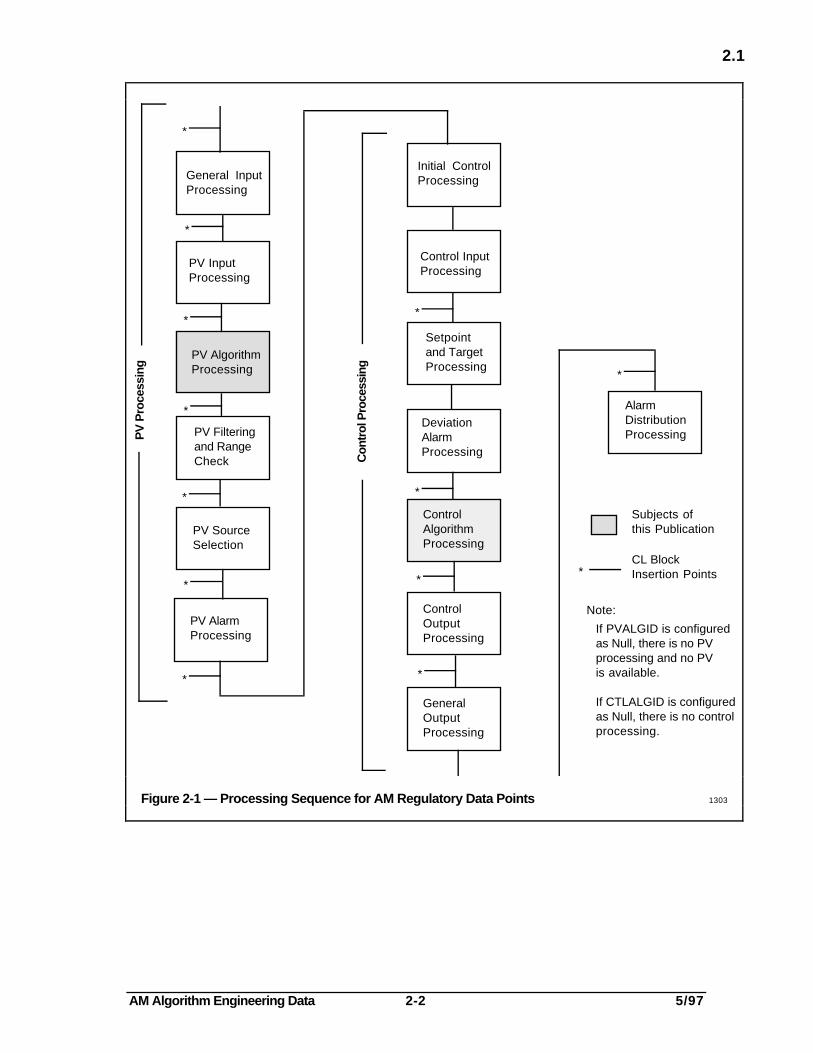
As Figure 2-1 shows, PV algorithm execution takes place between the PV-input-processingstep and the PV-filtering step in the regulatory data-point sequence. Control-algorithmexecution takes place between deviation-alarm processing and control output-processing.If a data point uses a PV algorithm and a PID control algorithm, the PV calculated by thePV algorithm is usually used by the control algorithm.
Each of Sections 3 through 23 defines one algorithm. PV algorithms are described inSections 3 through 12. Control algorithms are described in Sections 14 through 23.
Each of the algorithm descriptions has the same form and the same headings:
TYPE AND NAME
FUNCTION
USE
OPTIONS AND SPECIAL FEATURES
EQUATIONS
INITIALIZATION
OVERRIDE FEEDBACK PROCESSING
MIGRATION
Of these headings, Initialization and Override Feedback Processing do not apply to PValgorithms, so they are not included in Sections 3 through 13.
Each of the algorithm descriptions mentions several parameters associated with thealgorithm. The parameter names consist of CAPITAL letters. References to parametersnot named in the descriptions are provided after the descriptions. Further information onall data-point parameters, including the data type, range, and access keys, is provided in theApplication Module Parameter Reference Dictionary.
AM Algorithm Engineering Data 2-2 5/97
2.1
PV InputProcessing
PV AlgorithmProcessing
PV Filteringand RangeCheck
PV SourceSelection
PV AlarmProcessing
Initial ControlProcessing
Control InputProcessing
Setpointand TargetProcessing
DeviationAlarmProcessing
ControlAlgorithmProcessing
GeneralOutputProcessing
AlarmDistributionProcessing
ControlOutputProcessing
General InputProcessing
*
*
*
*
*
*
*
PV
Pro
cess
ing
*
*
*
*
*
Con
trol
Pro
cess
ing
Subjects ofthis Publication
*CL BlockInsertion Points
Note:
If PVALGID is configuredas Null, there is no PVprocessing and no PVis available.
If CTLALGID is configuredas Null, there is no controlprocessing.
Figure 2-1 — Processing Sequence for AM Regulatory Data Points 1303

AM Algorithm Engineering Data 3-1 5/97
3
DATA ACQUISITION (PV)Section 3
3.1 TYPE AND NAME
PV Algorithm: DATAACQ
3.2 FUNCTION
This algorithm normally accepts the input and places it, unchanged, in PVCALC. All ofthe other PV algorithms alter the input(s) in some way. See Figure 3-1.
3.3 USE
The most common use of this algorithm is to provide a PV that has been through GeneralInput Processing, PV Input Processing, PV Algorithm Processing, PV Filtering, and PVSource Selection (see Figure 2-1). The value in PVCALC is filtered, and becomes PV, ifthe PV source is AUTO.
The input can be a measured process-variable, or the calculated PV or calculated output ofanother data point. This algorithm could also be used to receive a calculated variable from aCL block, through a custom data segment.
The input to this algorithm and its output are in engineering units; for example, atemperature in °C from a thermocouple input to a Process Interface Unit (PIU).
3.4 OPTIONS AND SPECIAL FEATURES
This algorithm has no options nor special features.
3.5 EQUATION
There is only one equation. The operation is simply the replacement of the data point'scalculated PV (PVCALC) with the value of the input:
PVCALC = P1
Where P1 contains the first input value and PVCALC contains the value that becomes thePV when PVSOURCE = AUTO.
The parameters associated with with this algorithm are P1, PVCALC, and P1STS. Referto the Application Module Parameter Reference Dictionary.

AM Algorithm Engineering Data 3-2 5/97
3.6
MeasuredProcess Valueor Calculated Value fromAnother DataPoint
(Data Point Parameter)
PVCALC P1 DATAACQ
Figure 3-1 — Functional Diagram, Data Acquisition PV Algorithm 1304
3.6 MIGRATION
This Data Acquisition PV algorithm is like several similar PV algorithms inSUPERVISORY/TOTAL Systems and PMX Systems. The Hiway Gateway converts allprocess variables from the process-connected boxes, to engineering-units form, so onlyone Data Acquisition PV algorithm is needed in the AM.
Because the process-variable data supplied to SUPERVISORY/TOTAL and PMX Systemsis not in such consistent form, several data-acquisition PV algorithms are used. Thosealgorithms are
PV0 – LinearPV1 – Thermocouple Type JPV2 – Thermocouple Type KPV3 – Thermocouple Type TPV4 – Thermocouple Type SPV5 – Square Root LinearizationPV6 – 100 Ohm RTD*PV7 – RH Radiamatic*PV20 – Simple via Input WordPV21 – Simple via Input SourcePV103 – 10 Ohm Copper RTD*PV104 – E Type Thermocouple Transmitter*PV105 – R Type Thermocouple Transmitter*
*Not available in PMX Systems.

AM Algorithm Engineering Data 4-1 5/97
4
FLOW COMPENSATION (PV)Section 4
4.1 TYPE AND NAME
PV Algorithm: FLOWCOMP
4.2 FUNCTION
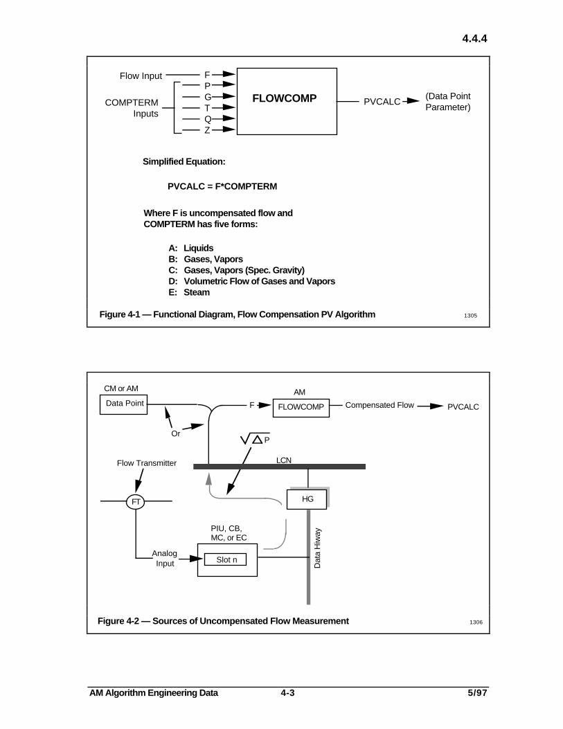
This algorithm compensates a flow measurement for variations in temperature, absolutepressure, specific gravity, or molecular weight. The measured flow can be that of a gas, avapor, or a liquid. An extended equation is provided for industrial steam-flowcompensation, which includes factors that compensate for steam quality andcompressibility. See Figure 4-1.
4.3 USE
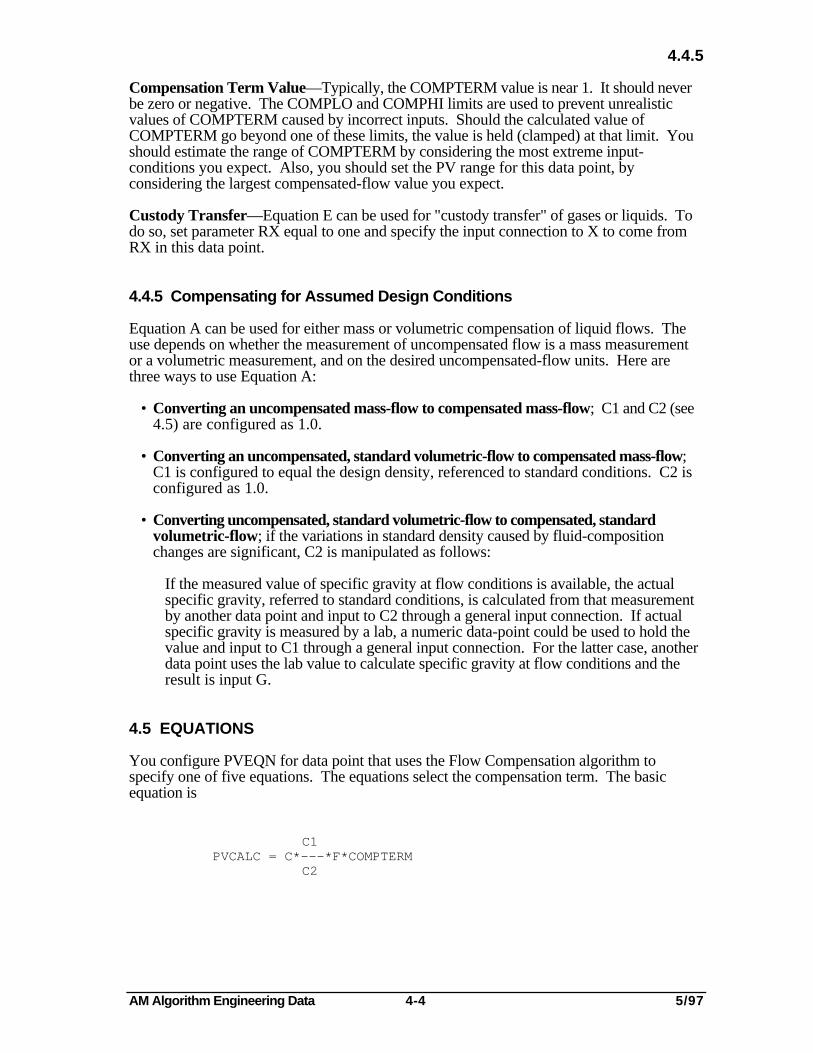
The uncompensated-flow input is typically a square-rooted, differential pressuremeasurement. Other direct-flow measurements can also be used. The square root shouldbe extracted before the input to this data point, and the input value must be in engineeringunits. For process-connected inputs, the square root can be extracted in the process-connected box, and conversion to EUs can take place in the Hiway Gateway. See Figure4-2.
The compensation is calculated from temperature, pressure, specific gravity, molecularweight, steam quality, or steam compressibility. Which of these is used depends on thetype of compensation you choose. All of these inputs are obtained through PV input-connections.
4.4 OPTIONS AND SPECIAL FEATURES
4.4.1 Five Forms of Flow Compensation
Parameter PVEQN specifies one of five different equations for this algorithm. Theequation causes the compensation term (COMPTERM) to differ according to theapplication, as follows (see 4.4.5 for the actual equations):
Equation A
Primarily used for mass-flow or volumetric-flow compensation for liquids. Actual(measured or calculated) specific gravity is used as a compensation input.
Equation B
Primarily used for mass-flow compensation of gas or vapor flows. Actual absolutetemperature and pressure are used as compensation inputs.
AM Algorithm Engineering Data 4-2 5/97
4.4.2
Equation C
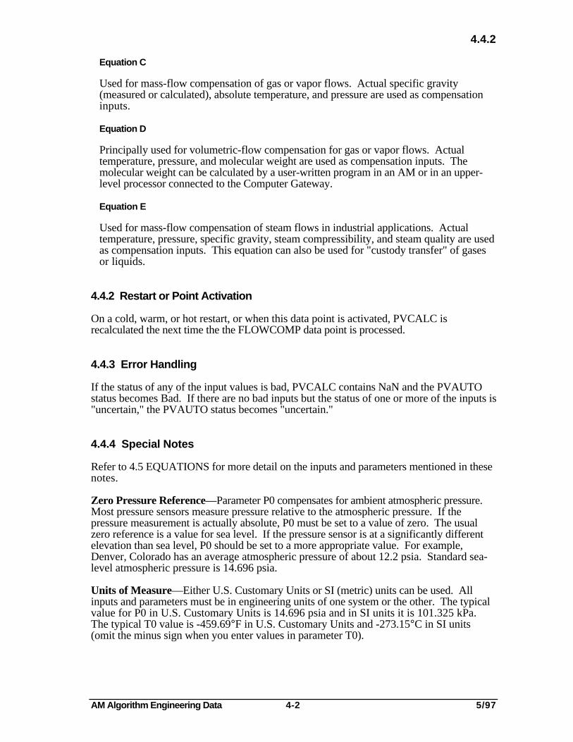
Used for mass-flow compensation of gas or vapor flows. Actual specific gravity(measured or calculated), absolute temperature, and pressure are used as compensationinputs.
Equation D
Principally used for volumetric-flow compensation for gas or vapor flows. Actualtemperature, pressure, and molecular weight are used as compensation inputs. Themolecular weight can be calculated by a user-written program in an AM or in an upper-level processor connected to the Computer Gateway.
Equation E
Used for mass-flow compensation of steam flows in industrial applications. Actualtemperature, pressure, specific gravity, steam compressibility, and steam quality are usedas compensation inputs. This equation can also be used for "custody transfer" of gasesor liquids.
4.4.2 Restart or Point Activation
On a cold, warm, or hot restart, or when this data point is activated, PVCALC isrecalculated the next time the the FLOWCOMP data point is processed.
4.4.3 Error Handling
If the status of any of the input values is bad, PVCALC contains NaN and the PVAUTOstatus becomes Bad. If there are no bad inputs but the status of one or more of the inputs is"uncertain," the PVAUTO status becomes "uncertain."
4.4.4 Special Notes
Refer to 4.5 EQUATIONS for more detail on the inputs and parameters mentioned in thesenotes.
Zero Pressure Reference—Parameter P0 compensates for ambient atmospheric pressure.Most pressure sensors measure pressure relative to the atmospheric pressure. If thepressure measurement is actually absolute, P0 must be set to a value of zero. The usualzero reference is a value for sea level. If the pressure sensor is at a significantly differentelevation than sea level, P0 should be set to a more appropriate value. For example,Denver, Colorado has an average atmospheric pressure of about 12.2 psia. Standard sea-level atmospheric pressure is 14.696 psia.
Units of Measure—Either U.S. Customary Units or SI (metric) units can be used. Allinputs and parameters must be in engineering units of one system or the other. The typicalvalue for P0 in U.S. Customary Units is 14.696 psia and in SI units it is 101.325 kPa.The typical T0 value is -459.69°F in U.S. Customary Units and -273.15°C in SI units(omit the minus sign when you enter values in parameter T0).
AM Algorithm Engineering Data 4-3 5/97
4.4.4
FPGTQZ
Flow Input
COMPTERMInputs
PVCALC(Data PointParameter)
Simplified Equation:
PVCALC = F*COMPTERM
Where F is uncompensated flow andCOMPTERM has five forms:
A: LiquidsB: Gases, VaporsC: Gases, Vapors (Spec. Gravity)D: Volumetric Flow of Gases and VaporsE: Steam
FLOWCOMP
Figure 4-1 — Functional Diagram, Flow Compensation PV Algorithm 1305
CM or AM
Data PointAM
FLOWCOMP Compensated Flow PVCALC
OrP
F
Dat
a H
iway
LCN
Slot n
FT
Flow Transmitter
AnalogInput
PIU, CB, MC, or EC
HG
Figure 4-2 — Sources of Uncompensated Flow Measurement 1306
AM Algorithm Engineering Data 4-4 5/97
4.4.5
Compensation Term Value—Typically, the COMPTERM value is near 1. It should neverbe zero or negative. The COMPLO and COMPHI limits are used to prevent unrealisticvalues of COMPTERM caused by incorrect inputs. Should the calculated value ofCOMPTERM go beyond one of these limits, the value is held (clamped) at that limit. Youshould estimate the range of COMPTERM by considering the most extreme input-conditions you expect. Also, you should set the PV range for this data point, byconsidering the largest compensated-flow value you expect.
Custody Transfer—Equation E can be used for "custody transfer" of gases or liquids. Todo so, set parameter RX equal to one and specify the input connection to X to come fromRX in this data point.
4.4.5 Compensating for Assumed Design Conditions
Equation A can be used for either mass or volumetric compensation of liquid flows. Theuse depends on whether the measurement of uncompensated flow is a mass measurementor a volumetric measurement, and on the desired uncompensated-flow units. Here arethree ways to use Equation A:
• Converting an uncompensated mass-flow to compensated mass-flow; C1 and C2 (see4.5) are configured as 1.0.
• Converting an uncompensated, standard volumetric-flow to compensated mass-flow;C1 is configured to equal the design density, referenced to standard conditions. C2 isconfigured as 1.0.
• Converting uncompensated, standard volumetric-flow to compensated, standardvolumetric-flow; if the variations in standard density caused by fluid-compositionchanges are significant, C2 is manipulated as follows:
If the measured value of specific gravity at flow conditions is available, the actualspecific gravity, referred to standard conditions, is calculated from that measurementby another data point and input to C2 through a general input connection. If actualspecific gravity is measured by a lab, a numeric data-point could be used to hold thevalue and input to C1 through a general input connection. For the latter case, anotherdata point uses the lab value to calculate specific gravity at flow conditions and theresult is input G.
4.5 EQUATIONS
You configure PVEQN for data point that uses the Flow Compensation algorithm tospecify one of five equations. The equations select the compensation term. The basicequation is
C1PVCALC = C*———*F*COMPTERM
C2
AM Algorithm Engineering Data 4-5 5/97
4.5
Where:
PVCALC = The output of this algorithm. It is selected as the PV for this data pointwhen the PV source is AUTOmatic.
C = Scale factor. The default value is 1.0.
C1, C2 = Constants for correcting for assumed design conditions. See 4.4.5.Default value for each is 1.0.
F = The uncompensated flow input. A square-rooted, differential pressure input.
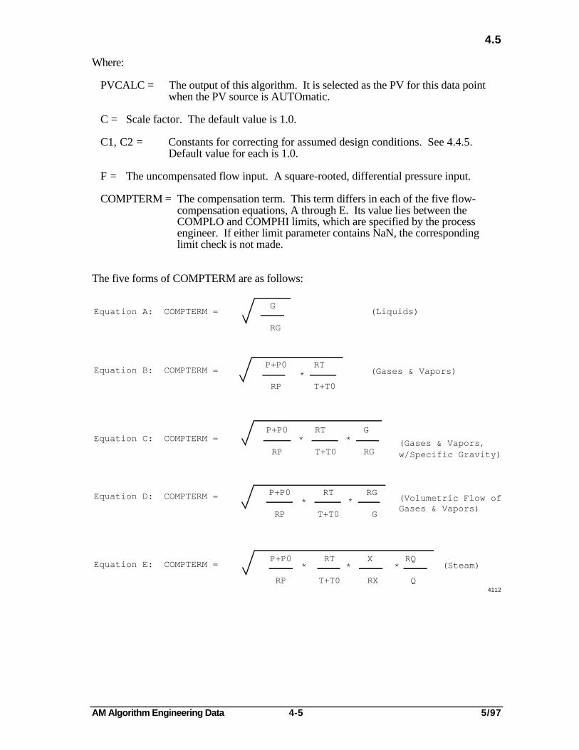
COMPTERM = The compensation term. This term differs in each of the five flow-compensation equations, A through E. Its value lies between theCOMPLO and COMPHI limits, which are specified by the processengineer. If either limit parameter contains NaN, the correspondinglimit check is not made.
The five forms of COMPTERM are as follows:
Equation A: COMPTERM =G
RG
(Liquids)
Equation D: COMPTERM = P+P0 RT RG RP T+T0 G
(Volumetric Flow ofGases & Vapors)
Equation C: COMPTERM =P+P0 RT G RP T+T0 RG
(Gases & Vapors,w/Specific Gravity)
Equation B: COMPTERM =P+P0 RT RP T+T0
(Gases & Vapors)
Equation E: COMPTERM =P+P0 RT X RQ RP T+T0 RX Q
(Steam)
*
**
*
*
* * *
4112
AM Algorithm Engineering Data 4-6 5/97
4.6
Where the following (in engineering units) are received through input connections
G = Measured or calculated specific gravity or molecular weight.
P = Measured actual gage pressure.
T = Measured actual temperature.
X = Measured actual steam compressibility.
Q = Measured actual steam-quality factor.
And the following parameters are specified by the process engineer
RG = Reference specific gravity or reference molecular weight, in the sameengineering units as G (Default value = 1.0).
RP = Reference pressure, in the same engineering units as P (Default value = 1.0).
RT = Reference temperature, in the same engineering units as T (default value = 1.0).
P0 = Zero reference for pressure, in the same engineering units as P. Typically14.696 psia or 101.325 kPa. See 4.4.4. Default value = 0.
T0 = Zero reference for temperature, in the same engineering units as T. Typically -459.69°F or -273.15°C (omit the minus sign when entering a value in T0). See4.4.4. Default value = 0.
RX = Reference steam compressibility, in the same engineering units as X. Defaultvalue = 1.0.
Other parameters associated with this algorithm are as follows (refer to the ApplicationModule Parameter Reference Dictionary):
FSTS QSTS COMPTERMGSTS XSTS PVCALCPSTS COMPLOLM PVEQNTSTS COMPHILM
4.6 MIGRATION
This Flow Compensation PV algorithm is like several similar PV algorithms inSUPERVISORY/TOTAL Systems and PMX Systems. The different forms of flowcompensation are necessary in SUPERVISORY/TOTAL and PMX Systems toaccommodate inputs in differing forms. The Hiway Gateway converts all process variablesfrom the process-connected boxes, to engineering-units form, so only one FlowCompensation PV algorithm is needed in the AM.
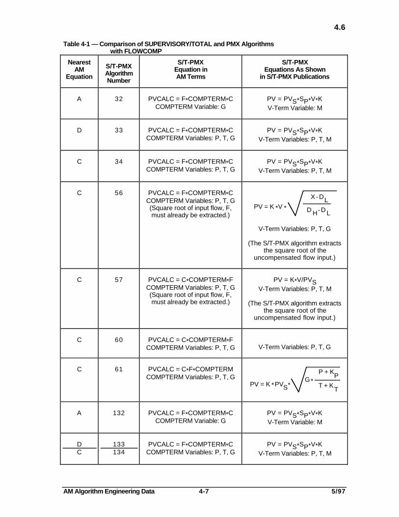
Table 4-1 compares the AM Flow Compensation PV algorithm with the flow-compensationalgorithms in SUPERVISORY/TOTAL and PMX Systems.
AM Algorithm Engineering Data 4-7 5/97
4.6
Table 4-1 — Comparison of SUPERVISORY/TOTAL and PMX Algorithmswith FLOWCOMP
NearestAM
Equation
S/T-PMXAlgorithmNumber
S/T-PMXEquation inAM Terms
S/T-PMXEquations As Shown
in S/T-PMX Publications
A 32 PVCALC = F*COMPTERM*CCOMPTERM Variable: G
PV = PVS*SP*V*KV-Term Variable: M
D 33 PVCALC = F*COMPTERM*CCOMPTERM Variables: P, T, G
PV = PVS*SP*V*KV-Term Variables: P, T, M
C 34 PVCALC = F*COMPTERM*CCOMPTERM Variables: P, T, G
PV = PVS*SP*V*KV-Term Variables: P, T, M
C 56 PVCALC = F*COMPTERM*CCOMPTERM Variables: P, T, G(Square root of input flow, F,must already be extracted.)
X - DL
D - DH LPV = K *V *
V-Term Variables: P, T, G
(The S/T-PMX algorithm extractsthe square root of the
uncompensated flow input.)
C 57 PVCALC = C*COMPTERM*FCOMPTERM Variables: P, T, G(Square root of input flow, F,must already be extracted.)
PV = K*V/PVSV-Term Variables: P, T, M
(The S/T-PMX algorithm extractsthe square root of the
uncompensated flow input.)
C 60 PVCALC = C*COMPTERM*FCOMPTERM Variables: P, T, G V-Term Variables: P, T, G
C 61 PVCALC = C*F*COMPTERMCOMPTERM Variables: P, T, G
P + KP
T + KT
PV = K *PVS*G*
A 132 PVCALC = F*COMPTERM*CCOMPTERM Variable: G
PV = PVS*SP*V*KV-Term Variable: M
DC
133134
PVCALC = F*COMPTERM*CCOMPTERM Variables: P, T, G
PV = PVS*SP*V*KV-Term Variables: P, T, M

AM Algorithm Engineering Data 4-8 5/97
AM Algorithm Engineering Data 5-1 5/97
5
GENERAL LINEARIZATION (PV)Section 5
5.1 TYPE AND NAME
PV Algorithm: GENLIN
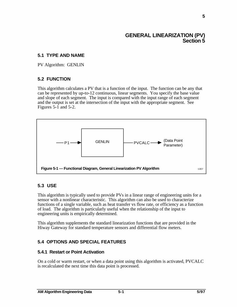
5.2 FUNCTION
This algorithm calculates a PV that is a function of the input. The function can be any thatcan be represented by up-to-12 continuous, linear segments. You specify the base valueand slope of each segment. The input is compared with the input range of each segmentand the output is set at the intersection of the input with the appropriate segment. SeeFigures 5-1 and 5-2.
GENLINP1 PVCALC(Data PointParameter)
Figure 5-1 — Functional Diagram, General Linearization PV Algorithm 1307
5.3 USE
This algorithm is typically used to provide PVs in a linear range of engineering units for asensor with a nonlinear characteristic. This algorithm can also be used to characterizefunctions of a single variable, such as heat transfer vs flow rate, or efficiency as a functionof load. The algorithm is particularly useful when the relationship of the input toengineering units is empirically determined.
This algorithm supplements the standard linearization functions that are provided in theHiway Gateway for standard temperature sensors and differential flow meters.
5.4 OPTIONS AND SPECIAL FEATURES
5.4.1 Restart or Point Activation
On a cold or warm restart, or when a data point using this algorithm is activated, PVCALCis recalculated the next time this data point is processed.
AM Algorithm Engineering Data 5-2 5/97
5.4.2
5.4.2 Error Handling
If the status of the P1 input is "uncertain," the PVAUTO status becomes "uncertain."
If the status of the P1 input is bad or if any of the segment coordinates (INi or OUTi)contains NaN, the PVAUTO-value status becomes bad.
If any of the segment coordinate values (INi or OUTi) contains NaN, a configuration alarmis generated.
5.4.3 Changing Parameters through a Universal Station
The SEGTOT, INi, and OUTi parameters can be changed through a Universal Station onlyif the data point that uses the GENLIN algorithm is made inactive.
5.4.4 Parameter—Value Restrictions
The input coordinate value parameters must be specified in ascending order from thesmallest value to the largest.
5.4.5 Extension of First and Last Segments
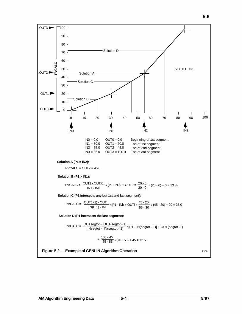
The first and last segments are treated as if they indefinitely extended, so if P1 is less thanIN0 or greater than INsegtot (see 5.5), PVCALC is computed by assuming that the slopeof the appropriate segment continues to the intersection point.
5.5 EQUATION
Each time this algorithm is processed the input value P1 is compared with each segment,starting with the first and continuing until a segment is found that intersects with the input.When that segment is found, PVCALC is calculated as follows:
• If the P1 value is exactly equal to the input value at the beginning of any segment (P1 =INi, for i in a range from 0 to the value in SEGTOT),
PVCALC = OUTi
• If P1 intersects the first segment (P1 < IN1),
OUT1 - OUT0PVCALC = ———————————*(P1 - IN0) + OUT0
IN1 - IN0

AM Algorithm Engineering Data 5-3 5/97
5.6
• If P1 intersects any segment except the first one or the last one [INi < P1 < IN(i+1) forany i from 1 to segtot-2],
(i+1)PV CALC =
OUT - OUTi*
IN (i+1)
IN1 (P1 - INi) + OUTi
• If P1 intersects the last segment [P1 > IN(segtot-1)],
+PVCALC =
OUTsegtot - OUT(segtot-1)
INsegtot - IN (segtot-1)* [P1 - IN
(segtot-1)] OUT
(segtot-1)
Where:
PVCALC = The output of this algorithm. It is selected as the PV for this data pointwhen the PV source is AUTOmatic.
P1 = The input value.
IN(i) = Input value at the beginning of the intersecting segment.
IN(i+1) = Input value at the end of the intersecting segment.
OUT(i) = Output value at the beginning of the intersecting segment.
OUT(i+1) = Output value at the end of the intersecting segment.
segtot = A subscript indicating the user-entered value in SEGTOT.
Other parameters associated with the GENLIN algorithm are as follows (refer to theApplication Module Parameter Reference Dictionary):
P1STS PVCALC SEGTOT
5.6 MIGRATION
There are no similar algorithms in PMX and SUPERVISORY/TOTAL Systems.
The Extended Controller has a similar algorithm that offers up-to-eight segments.
AM Algorithm Engineering Data 5-4 5/97
5.6
100
90
80
70
60
50
40
30
20
10
0
-
-
-
-
-
-
-
-
-
-
-
OUT3
PV
CA
LC
OUT2
OUT1
OUT0
0 10 20 30 40 50 60 70 80 90 100
IN0 IN1 IN2 IN3
IN0 = 0.0IN1 = 30.0IN2 = 55.0IN3 = 85.0
OUT0 = 0.0OUT1 = 20.0OUT2 = 45.0OUT3 = 100.0
Beginning of 1st segmentEnd of 1st segmentEnd of 2nd segmentEnd of 3rd segment
Solution A
Solution B
Solution C
SEGTOT = 3
Solution D
Solution A (P1 = IN2):
PVCALC = OUT2 = 45.0
Solution B (P1 > IN1):
PVCALC = OUT1 - OUT 0IN1 - IN0
(P1 -IN0) + OUT0 =
Solution C (P1 intersects any but 1st and last segment):
(45 - 30) + 20 = 35.0OUT(i+1) - OUTi
IN(I+1) - INI (P1 - INi) + OUTi =
45 - 20
55 - 30PVCALC =
Solution D (P1 intersects the last segment):
PVCALC = OUTsegtot - OUT(segtot - 1)
INsegtot - IN(segtot - 1) *[P1 - IN(segtot - 1)] + OUT(segtot -1)
= 100 - 4585 - 55 (70 - 55) + 45 = 72.5
*
* *
20 - 030 - 0 * (20 - 0) + 0 = 13.33
*
Figure 5-2 — Example of GENLIN Algorithm Operation 1308

AM Algorithm Engineering Data 6-1 5/97
6
HIGH SELECTOR, LOW SELECTOR, AVERAGE (PV)Section 6
6.1 TYPE AND NAME
PV Algorithm: HILOAVG
6.2 FUNCTION
This algorithm does one of the following:
• Selects the input with the highest value
• Selects the input with the lowest value
• Calculates the average value of all valid inputs
It can accept up-to-eight inputs. Valid inputs are those whose status is "Normal" or"Uncertain." When the input selection functions are used, the number of the input that isselected is contained in an accessible parameter (SELINP). See Figure 6-1.
6.3 USE
One example of the use of this algorithm is shown at the top of Figure 6-1. In thisexample, the high value-selector version of the algorithm is used to detect hot spots in aboiler or a reactor.
Either the high value-selector version or the low value-selector version can be used to detectproduction bottlenecks. For example, this algorithm might be used to notify the processoperator that production is currently constrained by the speed of a gas compressor. One ofthe selector options might also be used to select the "safest" PV for control.
One use of the averaging option is in balancing furnace passes. In this application, thealgorithm calculates the average of the outlet temperatures of the passes.
6.4 OPTIONS AND SPECIAL FEATURES
6.4.1 Forced Selection
The data point can be configured to allow the Universal Station operator, a user-writtenprogram, or a general-input connection to force selection of one of the inputs.

AM Algorithm Engineering Data 6-2 5/97
6.4.1
Example:
Which is the hottest spotin the boiler?
P1P2P3P4P5P6P7P8
HILOAVG
Eq. A
PVCALC
SELINP
(Data PointParameters)
P1P2P3P4P5P6P7P8
HILOAVG
Eq. B
PVCALC
SELINP
(Data PointParameters)
P1P2P3P4P5P6P7P8
HILOAVG
Eq. CPVCALC (Data Point
Parameters)
PVCALC = Highest of the Input Values
PVCALC = Lowest of the Input Values
PVCALC = Average of all Valid Input Values
PVCALC = (P1 + . . . . . . . + P ) / NN
Where N = the number of valid inputs.
Figure 6-1 — Functional Diagram, HI, LO, Average Selector PV Algorithm 3670
AM Algorithm Engineering Data 6-3 5/97
6.4.2
• If the FRCPERM parameter is configured as On, the forced-selection function isenabled and an operator, a user-written program, or a general input connection canforce the selection.
• IF FRCPERM is configured as Off, the forced-selection function is disabled.
The FSELIN parameter specifies the input to be selected, when selection is forced(SelectP1 through SelectP8).
6.4.2 Error Handling
Except when forced selection is in effect (6.4.1), inputs with a bad status are ignored andthey do not make the PVAUTO status bad. For example, if the algorithm is configured as a4-input high selector and one of the inputs goes bad, the algorithm functions as a 3-inputhigh-selector.
If the number of valid inputs (PV status of good or uncertain) is less than the minimumnumber specified in parameter NMIN, PVCALC becomes NaN and the PVAUTO status isbad.
The value status of PVAUTO is changed to uncertain under any of the followingconditions:
• An input selection is forced and the status of that input is not bad (is normal oruncertain).
• Forced selection is not in effect, at least as many inputs as specified by NMIN arenormal or uncertain, and the status of the selected one (Equation A or B) is uncertain.
• Equation C (averaging) is chosen, at least as many inputs as specified by NMIN are notbad (normal or uncertain), and the status of any of them is uncertain.
PVCALC becomes NaN and the PVAUTO value-status becomes bad under either of thefollowing conditions:
• The selection of an input is forced and the status of that input is bad.
• Forced selection is not in effect, and there are fewer inputs with a status other than badthan are specified by NMIN.
6.4.3 Restart or Point Activation
On a cold, warm, or hot restart, or when this data point is activated, PVCALC is simplyrecalculated the next time this data point is processed.
6.5 EQUATIONS
Equation A selects the highest input value. Equation B selects the lowest input value.Equation C calculates the average of all valid inputs.
AM Algorithm Engineering Data 6-4 5/97
6.6
Equation A—High Selector
If FRCPERM and FORCE are both On,
PVCALC = the value of the input indicated by FSELIN and
SELINP = FSELIN
If either FRCPERM or FORCE is Off,
PVCALC = the highest valid input.
SELINP = the selected input, SelectP1 through SelectP8.
Equation B—Low Selector
If FRCPERM and FORCE are both On,
PVCALC = the value of the input indicated by FSELIN and
SELINP = FSELIN
If either FRCPERM or FORCE is Off,
PVCALC = the lowest valid input.
SELINP = the selected input, SelectP1 through SelectP8.
Equation C—Average
If FRCPERM and FORCE are both On,
PVCALC = the value of the input indicated by FSELIN and
SELINP = FSELIN
If either FRCPERM or FORCE is Off,
PVCALC = (Sum of the valid inputs)/N
SELINP = None
Other parameters associated with the HILOAVG algorithm are as follows (refer to theApplication Module Parameter Reference Dictionary):
NMIN PVEQNPnSTS SELINP
6.6 MIGRATION
There are no similar algorithms in PMX and SUPERVISORY/TOTAL Systems.

AM Algorithm Engineering Data 7-1 5/97
7
TOTALIZER (PV)Section 7
7.1 TYPE AND NAME
PV Algorithm: TOTALIZR
7.2 FUNCTION
This algorithm provides a time-scaled accumulation of a single-input value. The inputvalue is typically a flow measurement. The timebase can be seconds, minutes, or hours.
A data point that uses this algorithm cannot use a control algorithm.
The accumulation can be started, stopped, and reset by commands from a Universal Stationoperator or from a user-written program. An operator or user-written program canestablish a target value for the accumulation. Status indicators are available to indicate thatthe accumulation is near the target value, nearer to the target value, and is complete (hasreached or exceeded the target value).
For situations where the flow transmitter may not be precisely calibrated near the zero-flowvalue, a zero-flow cutoff feature is provided that avoids accumulating negative flow values.When the flow is below a user-specified cutoff value, the input value is clamped to zero.
Typically a flowmeasurement
Operator or user-written program
Equations A through F specify bad value andrestart-handling options. See 7.4.5
For all equations:PVCALC = PVCALC (i-1) + C (Time Scale) P1
P1
StartStop
ResetTIMEBASE
Target Value
TOTALIZR PVCALCTime-scaledaccumulation
Target valueflags
* *
Figure 7-1 — Functional Diagram, Totalizer PV Algorithm 1310
AM Algorithm Engineering Data 7-2 5/97
7.3
7.3 USE
The Totalizer PV algorithm accumulates periodic measurements over time. It is principallyused to accumulate total flows, or in applications such as the measurement of ingredientsthat are blended. The accumulated value can be used for control or just as process history.
An example of TOTALIZR's use in control is determining how full a tank is, so that theflow into the tank can be shut off before it overflows. In such an application, the P1 inputto TOTALIZR would be the PV of PID-flow controller.
7.4 OPTIONS AND SPECIAL FEATURES
7.4.1 Typical Operation
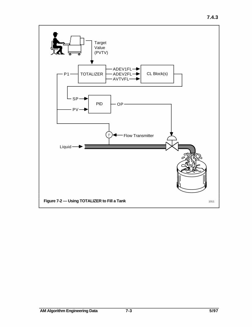
The events in an operation that uses TOTALIZR might be as follows (see Figure 7-2):
• The target value, which represents the desired total volume, is specified to the PVTVparameter in the TOTALIZR point, by an operator at a Universal Station or by a user-written program.
• An operator or a user-written program issues a RESET command to TOTALIZR point.This sets any accumulation value equal to RESETVAL.
• A START command is issued to the TOTALIZR point. A CL block inserted in theprocessing of one of the points uses the setpoint Target Value function (see 3.1.6.2 inAM Control Functions) in the PID point, to "ramp" the flow up to a steady rate.
• When the first "slowdown" or "near-target" flag (ADEV1FL) comes on, another CLblock ramps the flow SP down to a lower value.
• When the second "slowdown" or "near-target" flag (ADEV2FL) comes on, the flow SPis lowered to a trickle.
• When the accumulation reaches the target value, filling is complete and the completeflag (AVTVFL) comes on. A CL block shuts the flow off. The TOTALIZR point'sPV-high alarm can be configured to trip at this point, so the operator is notified thatfilling is complete.
7.4.2 Timebase and Engineering-Units Scaling
The user specifies the timebase in seconds, minutes, or hours, in parameter TIMEBASE.This is the timebase in which the flow measurement is made. For example, liters persecond.
Scale factor, C, can be used to convert from one set of engineering units to another, forexample, from gallons per minute to barrels per minute.
AM Algorithm Engineering Data 7-3 5/97
7.4.3
TOTALIZERADEV1FLADEV2FLAVTVFL
CL Block(s)
PIDSP
PV
TargetValue(PVTV)
P1
F
OP
Liquid
Flow Transmitter
Figure 7-2 — Using TOTALIZER to Fill a Tank 1311

AM Algorithm Engineering Data 7-4 5/97
7.4.3
7.4.3 Commands and States
Three commands can be issued to the data point that is using TOTALIZR from a UniversalStation or by a user-written program. These commands are written in the TOTALIZRpoint's COMMAND parameter. The commands are as follows:
• None—No action.
• Start—Start the accumulation. STATE changes to Running.
• Stop—Stop the accumulation. STATE changes to Stopped.
• Reset—Reset the accumulation value to a user-specified value. This value isspecified in parameter RSETVAL. If the accumulator is running, it continues from thereset value.
7.4.4 Near-Zero Cutoff
To prevent accumulation of negative flow values, where the flow transmitter may not beprecisely calibrated near zero flow, you can specify a cutoff value in parameterCUTOFFLM. When the P1 value is equal to or below CUTOFFLM, it is replaced by zero.You can eliminate this feature by specifying NaN in CUTOFFLM.
7.4.5 Target-Value Flags
The target value can be specified by an operator by storing it in PVTV. A user-writtenprogram can specify it by storing in AVTV. These parameters track each other. Thisfeature can be disabled by storing NaN in AVTV. NaN cannot be stored by a CL program;it must be done by the Operator.
When the accumulated value in PVCALC exceeds AVTV, the target-value-reached flag,AVTVFL, goes to On, indicating that the accumulation is complete.
Even if the accumulator has stopped, this check is made on each processing pass.
You can specify two other trip points in AVDEV1TP and AVDEV2TP. They are specifiedas deviations from AVTV. Each of them is associated with a flag:
AVDEV1FL trips when
PVCALC > AVTV - AVDEV1TP
AVDEV2FL trips when
PVCALC > AVTV - AVDEV2TP
When the accumulated value (PVAUTO) status is bad, AVTVFL, AVDEV1FL, andAVDEV2FL are all Off.

AM Algorithm Engineering Data 7-5 5/97
7.4.6
7.4.6 Bad-Input and Warm-Restart Options
You can configure equations A through F for this algorithm, but instead of specifying thecalculation, they specify combinations of the following five options:
• Use Zero—When the accumulator is running, if P1's value status goes bad, P1's valueis replaced by zero and the accumulation continues with the PVAUTO status uncertain.When P1 is again good, PVAUTO remains uncertain until a reset command is received.No special action by the operator is required.
• Use Last Good Value—When the accumulator is running, if P1's value status goesbad, P1's value is replaced by the last good value and the accumulation continues withthe PVAUTO status uncertain. When P1 is again good, PVAUTO remains uncertainuntil a reset command is received. No special action by the operator is required.
• Set PVAUTO Status Bad and Stop—When the accumulator is running, if P1's valuestatus goes bad, the value in PVCALC becomes NaN, the PVAUTO status goes badand the accumulator is stopped. If the PV source is AUTO, a bad-PV alarm isgenerated. When P1 is again normal, PVAUTO remains bad until the accumulator isstarted again. To restart the accumulation, the operator should estimate its value anduse the reset command (see 7.4.3) to establish that value, then use the Start commandto restart the accumulation. The last accumulated value before the status went bad is inLASTPV.
• Continue After a Warm Restart—On a warm restart when the accumulator is running,the accumulation continues from the last PVCALC value. The PVAUTO status goes touncertain and remains so until a reset command is received.
• Set PVAUTO Status Bad and Stop After a Warm Restart—On a warm restart when theaccumulator is running, the value in PVCALC becomes NaN, the PVAUTO status goesbad and the accumulation is stopped. The operator must intervene to restart theaccumulator.
These options are selected as follows:
Equation Bad Input Handling Warm Restart
A Use Zero Continue
B Use Last Good Value Continue
C Set Bad and Stop Continue
D Use zero Set Bad and Stop
E Use Last Good Value Set Bad and Stop
F Set Bad and Stop Set Bad and Stop
If the accumulator is stopped, the P1-value status is ignored. If the accumulator is stoppedon a warm restart, no special action by the operator is required.

AM Algorithm Engineering Data 7-6 5/97
7.4.7
7.4.7 Restart or Point Activation
When the TOTALIZR data point is activated or on a cold restart, the PVCALC valuebecomes NaN, PVAUTO status goes bad and the accumulator state is Stopped. If the PVsource is AUTO, this causes a bad-PV alarm and the operator must re-establish normaloperation.
The processing that takes place for a warm restart is described under 7.4.6.
7.4.8 Scheduling
A data point that uses TOTALIZR must be scheduled after the point that suppliesTOTALIZR's P1 input.
7.4.9 Error Handling
The PVAUTO value status is uncertain when
• The P1-value status is uncertain.
• The P1-value status is bad and "use zero" or "use last value" (Equations A, B, D, or E)is configured (see 7.4.6).
• The data point is in a warm restart and the continue option (Equations A, B, or C) isconfigured (see 7.4.6).
A reset command is needed to return the PVAUTO-value status to normal, provided the P1status is normal.
PVCALC contains NaN and the PVAUTO-value status is bad when
• The P1-value status is bad and "set bad and stop" (Equation C or F) is configured.
• The data point is in a warm restart and is configured for "set bad and stop" (EquationsD, E, or F) is configured.
A reset command is needed to return the PVAUTO-value status to normal, provided the P1status is normal.
AM Algorithm Engineering Data 7-7 5/97
7.5
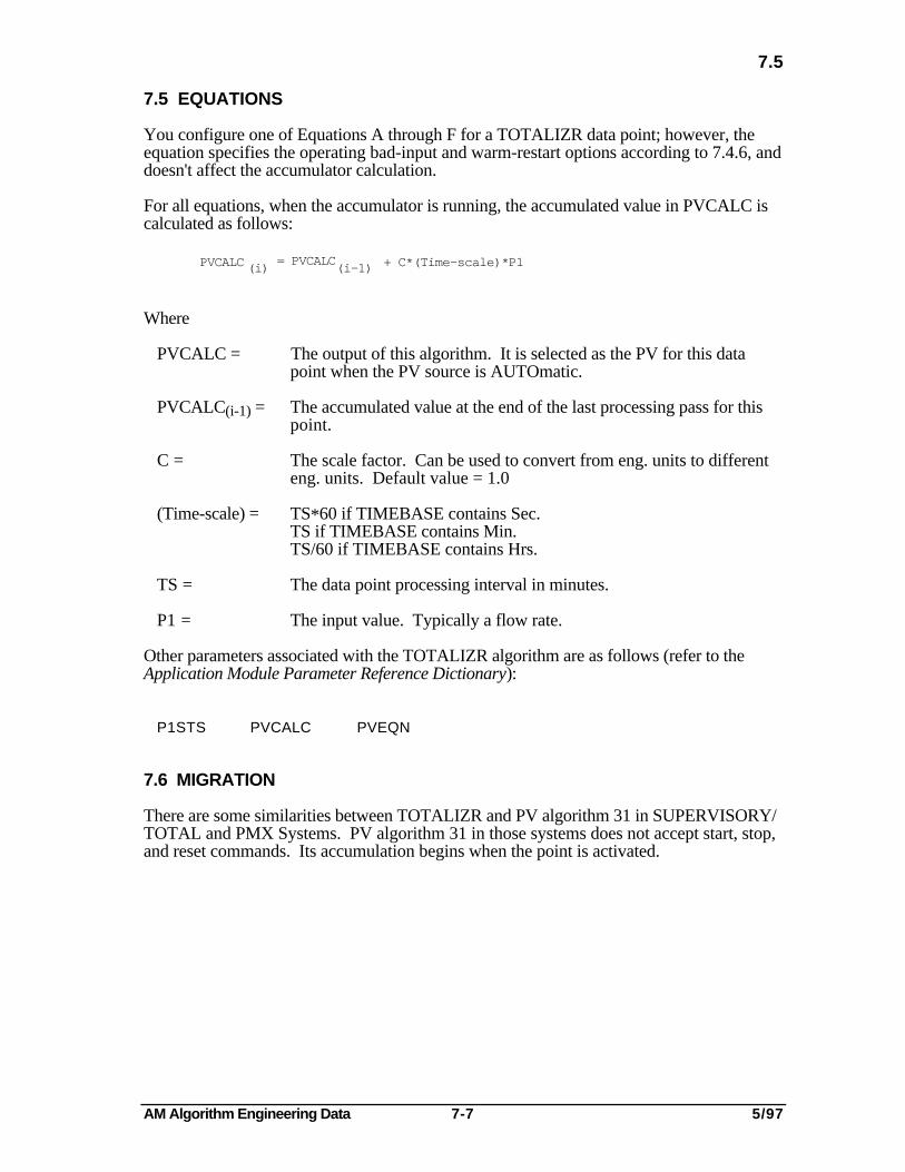
7.5 EQUATIONS
You configure one of Equations A through F for a TOTALIZR data point; however, theequation specifies the operating bad-input and warm-restart options according to 7.4.6, anddoesn't affect the accumulator calculation.
For all equations, when the accumulator is running, the accumulated value in PVCALC iscalculated as follows:
PVCALC (i)= PVCALC
(i-1) + C*(Time-scale)*P1
Where
PVCALC = The output of this algorithm. It is selected as the PV for this datapoint when the PV source is AUTOmatic.
PVCALC(i-1) = The accumulated value at the end of the last processing pass for thispoint.
C = The scale factor. Can be used to convert from eng. units to differenteng. units. Default value = 1.0
(Time-scale) = TS*60 if TIMEBASE contains Sec.TS if TIMEBASE contains Min.TS/60 if TIMEBASE contains Hrs.
TS = The data point processing interval in minutes.
P1 = The input value. Typically a flow rate.
Other parameters associated with the TOTALIZR algorithm are as follows (refer to theApplication Module Parameter Reference Dictionary):
P1STS PVCALC PVEQN
7.6 MIGRATION
There are some similarities between TOTALIZR and PV algorithm 31 in SUPERVISORY/TOTAL and PMX Systems. PV algorithm 31 in those systems does not accept start, stop,and reset commands. Its accumulation begins when the point is activated.

AM Algorithm Engineering Data 7-8 5/97

AM Algorithm Engineering Data 8-1 5/97
8
MIDDLE-OF-THREE SELECTOR (PV)Section 8
8.1 TYPE AND NAME
PV Algorithm: MIDOF3
8.2 FUNCTION
This algorithm provides a calculated PV (PVCALC) that is normally the middle value ofthree values from active PV-input connections. The PVAUTO status goes bad, only if allthree inputs to this algorithm are bad. If at least one input is valid (normal or uncertain),the algorithm provides a valid value in PVCALC. See Figure 8-1.
MIDOF3PVCALC
(Data PointParameter)
P1
P3
P2
SELINP
Normal Operation: PVCALC = Middle value of the three input values.
With only two valid inputs:
Equation A; PVCALC = Highest of the two inputs
Equation B; PVCALC = Lowest of the two inputs
Equation C; PVCALC = Average of the two inputs
With only one valid input: PVCALC = Value of the input
SELINP = The selected input, SelectP1 through SelectP3, except,with only two valid inputs and Eq. C, SELINP contains None.
Figure 8-1 — Functional Diagram, Middle-of-Three Selector PV Algorithm 1312
AM Algorithm Engineering Data 8-2 5/97
8.3
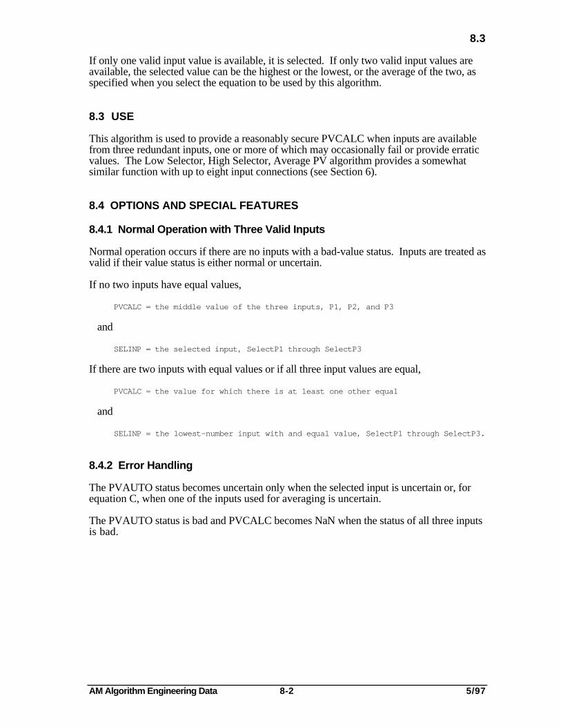
If only one valid input value is available, it is selected. If only two valid input values areavailable, the selected value can be the highest or the lowest, or the average of the two, asspecified when you select the equation to be used by this algorithm.
8.3 USE
This algorithm is used to provide a reasonably secure PVCALC when inputs are availablefrom three redundant inputs, one or more of which may occasionally fail or provide erraticvalues. The Low Selector, High Selector, Average PV algorithm provides a somewhatsimilar function with up to eight input connections (see Section 6).
8.4 OPTIONS AND SPECIAL FEATURES
8.4.1 Normal Operation with Three Valid Inputs
Normal operation occurs if there are no inputs with a bad-value status. Inputs are treated asvalid if their value status is either normal or uncertain.
If no two inputs have equal values,
PVCALC = the middle value of the three inputs, P1, P2, and P3
and
SELINP = the selected input, SelectP1 through SelectP3
If there are two inputs with equal values or if all three input values are equal,
PVCALC = the value for which there is at least one other equal
and
SELINP = the lowest-number input with and equal value, SelectP1 through SelectP3.
8.4.2 Error Handling
The PVAUTO status becomes uncertain only when the selected input is uncertain or, forequation C, when one of the inputs used for averaging is uncertain.
The PVAUTO status is bad and PVCALC becomes NaN when the status of all three inputsis bad.

AM Algorithm Engineering Data 8-3 5/97
8.5
8.5 EQUATIONS
If three valid inputs are present, the equations have no meaning and the algorithm functionsnormally, as described under 8.4.1. The equations specify what the algorithm is to do ifone or more inputs has a bad-value status. The equations function as follows:
• With one bad input
Equation A
PVCALC = Highest of the two input values
SELINP = The selected input, SelectP1 through SelectP3
Equation B
PVCALC = Lowest of the two input values
SELINP = The selected input, SelectP1 through SelectP3
Equation C
PVCALC = The average of the two input values
SELINP = None
• With two bad inputs
Equations A, and B
PVCALC = the value of the valid input
SELINP = The selected input, SelectP1 through SelectP3
Equation C
PVCALC = the value of the valid input
SELINP = None
• With three bad inputs
Equations A, B, and C
PVCALC = NaN
SELINP = None

AM Algorithm Engineering Data 8-4 5/97
8.6
Where:
PVCALC = The output of this algorithm. It is selected as the PV for the datapoint when the PV source is AUTOmatic.
P1, P2, and P3 = The input values. The default value is NaN.
SELINP = The selected input, SelectP1 through SelectP3. If no input isselected or if PVCALC contains an average value, SELINPcontains None.
Other parameters associated with the MIDOF3 algorithm are as follows (refer tothe Application Module Parameter Reference Dictionary):
P1STS P3STSP2STS PVEQN
8.6 MIGRATION
PV algorithm no. 54 in SUPERVISORY/TOTAL is similar to this algorithm with EquationB selected. There is a similar algorithm in the Extended Controller that selects the lower oftwo inputs if a third input is not available.
AM Algorithm Engineering Data 9-1 5/97
9
MULTIPLIER/DIVIDER (PV)Section 9
9.1 TYPE AND NAME
PV Algorithm: MULDIV
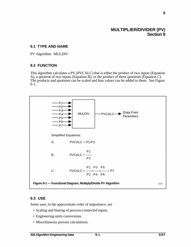
9.2 FUNCTION
This algorithm calculates a PV (PVCALC) that is either the product of two inputs (EquationA), a quotient of two inputs (Equation B), or the product of three quotients (Equation C).The products and quotients can be scaled and bias values can be added to them. See Figure9-1.
P1P2P3P4P5P6P7
MULDIV PVCALC (Data PointParameter)
Simplified Equations:
A; PVCALC = P1*P2
P1B; PVCALC = ——
P2
P1 P3 P5C; PVCALC = ——*——*—— + P7
P2 P4 P6
Figure 9-1 — Functional Diagram, Multiply/Divide PV Algorithm 1313
9.3 USE
Some uses, in the approximate order of importance, are
• Scaling and biasing of process-connected inputs.
• Engineering-units conversions.
• Miscellaneous process calculations.
AM Algorithm Engineering Data 9-2 5/97
9.4
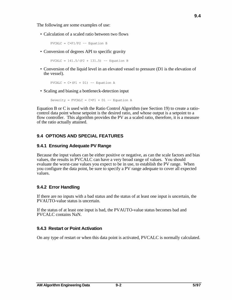
The following are some examples of use:
• Calculation of a scaled ratio between two flows
PVCALC = C*P1/P2 -- Equation B
• Conversion of degrees API to specific gravity
PVCALC = 141.5/(P2 + 131.5) -- Equation B
• Conversion of the liquid level in an elevated vessel to pressure (D1 is the elevation ofthe vessel).
PVCALC = C*(P1 + D1) -- Equation A
• Scaling and biasing a bottleneck-detection input
Severity = PVCALC = C*P1 + D1 -- Equation A
Equation B or C is used with the Ratio Control Algorithm (see Section 19) to create a ratio-control data point whose setpoint is the desired ratio, and whose output is a setpoint to aflow controller. This algorithm provides the PV as a scaled ratio, therefore, it is a measureof the ratio actually attained.
9.4 OPTIONS AND SPECIAL FEATURES
9.4.1 Ensuring Adequate PV Range
Because the input values can be either positive or negative, as can the scale factors and biasvalues, the results in PVCALC can have a very broad range of values. You shouldevaluate the worst-case values you expect to be in use, to establish the PV range. Whenyou configure the data point, be sure to specify a PV range adequate to cover all expectedvalues.
9.4.2 Error Handling
If there are no inputs with a bad status and the status of at least one input is uncertain, thePVAUTO-value status is uncertain.
If the status of at least one input is bad, the PVAUTO-value status becomes bad andPVCALC contains NaN.
9.4.3 Restart or Point Activation
On any type of restart or when this data point is activated, PVCALC is normally calculated.

AM Algorithm Engineering Data 9-3 5/97
9.5
9.5 EQUATIONS
You can select any one of three equations when configuring a data point that uses theMultiplier/Divider PV algorithm:
Equation A
PVCALC = C*(C1*P1 + D1)*(C2*P2 + D2) + D
Equation B
(C1*P1 + D1)PVCALC = C*———————————— + D
(C2*P2 + D2)
Equation C
(C1*P1 + D1) (C3*P3 + D3) (C5*P5 + D5)PVCALC = C*————————————*————————————*———————————— + (C7*P7 + D7) + D
(C2*P2 + D2) (C4*P4 + D4) (C6*P6 + D6)
Where:
PVCALC = The output of this algorithm. It is selected as the PV for the data pointwhen the PV source is AUTOmatic.
P1 through P7 = The input values. The P1 default value is NaN. Default values for P2through P6 are 1.0. For P7, the default value is 0.
C = The overall scale factor. The default value is 1.0.
D = The overall bias value. The default value is 0.
C1 through C7 = Scale factors for Pn inputs with the same number. The default valuefor each is 1.0.
D1 through D7 = Bias values for the scaled inputs with the same number. The defaultvalue for each is 0.
Other parameters associated with the MULDIV algorithms are as follows (refer to theApplication Module Parameter Reference Dictionary):
PnSTS PVEQN
AM Algorithm Engineering Data 9-4 5/97
9.6
9.6 MIGRATION
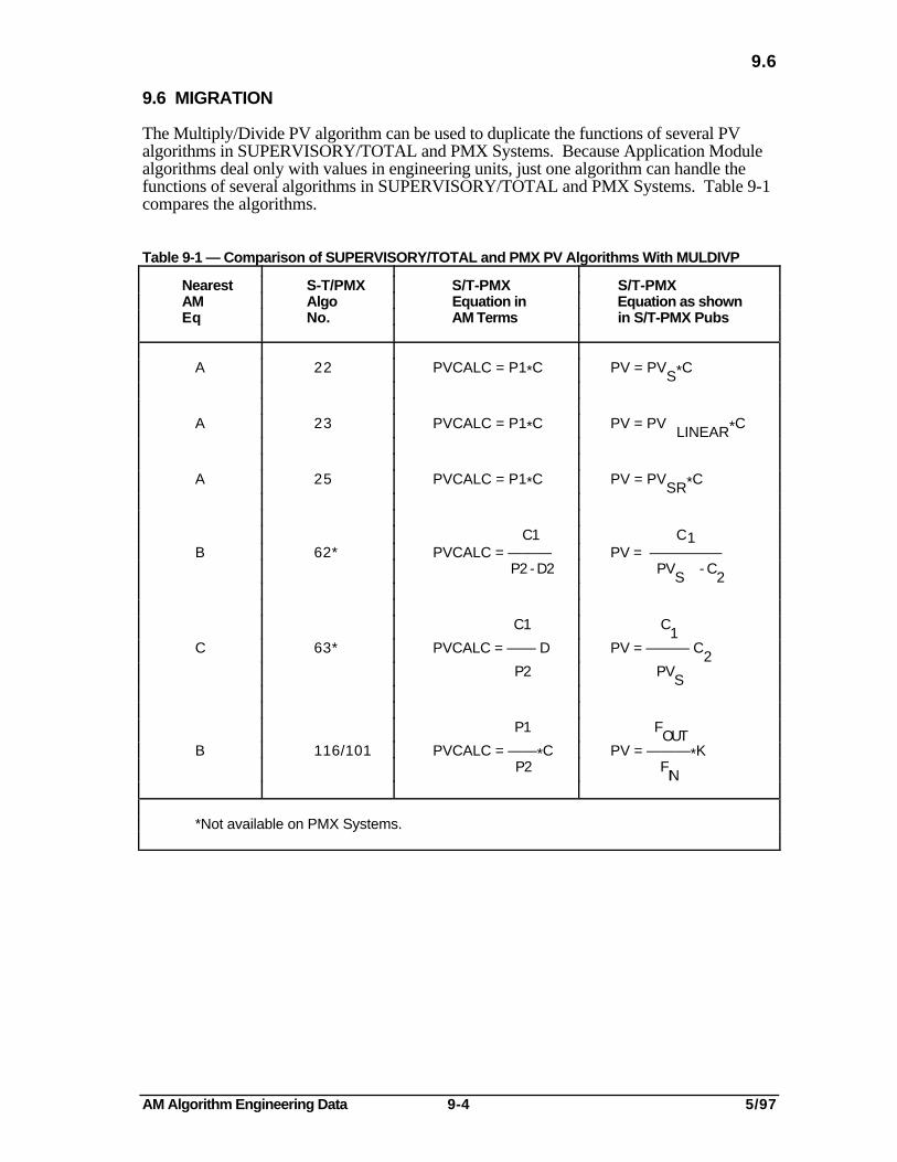
The Multiply/Divide PV algorithm can be used to duplicate the functions of several PValgorithms in SUPERVISORY/TOTAL and PMX Systems. Because Application Modulealgorithms deal only with values in engineering units, just one algorithm can handle thefunctions of several algorithms in SUPERVISORY/TOTAL and PMX Systems. Table 9-1compares the algorithms.
Table 9-1 — Comparison of SUPERVISORY/TOTAL and PMX PV Algorithms With MULDIVP
Nearest S-T/PMX S/T-PMX S/T-PMXAM Algo Equation in Equation as shownEq No. AM Terms in S/T-PMX Pubs
A 22 PVCALC = P1*C PV = PVS*C
A 23 PVCALC = P1*C PV = PVLINEAR*C
A 25 PVCALC = P1*C PV = PVSR*C
C1 C1B 62* PVCALC = ——— PV = —————
P2 - D2 PVS
- C2
C1 C1
C 63* PVCALC = —— D PV = ——— C2
P2 PVS
P1 FOUT
B 116/101 PVCALC = ——*C PV = ———*K P2 F
IN
*Not available on PMX Systems.

AM Algorithm Engineering Data 10-1 5/97
10
SUMMER (PV)Section 10
10.1 TYPE AND NAME
PV Algorithm: SUMMER
10.2 FUNCTION
This algorithm calculates a PV (PVCALC) that is the sum of up to eight input values. Theinput values can be scaled, the combined inputs can be scaled, and a bias value can beadded to the result. See Figure 10-1.
P1P2P3P4P5P6P7P8
SUMMER PVCALC (Data PointParameters)
Equation B, Simplified:
PVCALC = P1 + P2 + . . . + P8
Figure 10-1 — Functional Diagram, Summer PV Algorithm 1314
10.3 USE
A typical use is the calculation of the rate at which a component of a raw product is enteringa process unit, which is found by summing the proportion of the component in each ofseveral input streams and multiplying by the stream flow rates. This algorithm can also beused to calculate a net heat loss by finding the difference between the heat inputs and heatoutputs (the difference can be obtained by using a negative scale factor, for example,–1.0).
Other possible uses are mass-balance, heat-balance, and inventory calculations.

AM Algorithm Engineering Data 10-2 5/97
10.4
10.4 OPTIONS AND SPECIAL FEATURES
10.4.1 Ensuring Adequate PV Range
Because the input values can be either positive or negative, as can the scale factors and biasvalues, the results in PVCALC can have a very broad range of values. You shouldevaluate the worst-case values you expect to be in use, to establish the PV range. Whenyou configure the data point, be sure to specify a PV range adequate to cover all expectedvalues.
10.4.2 Error Handling
If there are no inputs with a bad status and the status of at least one input is uncertain, thePVAUTO-value status is uncertain.
If the status of at least one input is bad, the PVAUTO-value status becomes bad andPVCALC contains NaN.
10.4.3 Restart or Point Activation
On any type of restart or when this data point is activated, PVCALC is normally calculated.
10.5 EQUATIONS
You can select one of two equations when you configure a data point that uses the SummerPV algorithm:
Equation A
PVCALC = C*P1 + D
Equation B
PVCALC = C*(C1*P1 + C2*P2 + . . . . +Cn*Pn) + D
Where:
PVCALC = The output of this algorithm. It is selected as the PV for this data pointwhen the PV source is AUTOmatic.
C = The overall scale factor. Default = 1.0.
C1 through Cn = The scale factors for P1 through Pn. Default = 1.0.

AM Algorithm Engineering Data 10-3 5/97
10.6
P1 through Pn = The PV input values. Default for all values is NaN
D = The overall bias. Default = 0.
n = The number of PV inputs used. Default = 2.
Other parameters associated with the SUMMER algorithm are as follows (refer to theApplication Module Parameter Reference Dictionary):
N PnSTS PVEQN
10.6 MIGRATION
The Summer PV algorithm can accomplish the function of four similar algorithms inSUPERVISORY/TOTAL and PMX Systems. Table 10-1 compares those algorithms tothis one.
Table 10-1 — Comparison of SUPERVISORY/TOTAL Algorithms With SUMMER
NearestAM
Equation
S-T/PMXAlgorithmNumber
S-T/PMXEquation inAM Terms
S-T/PMXEquation as shownin S/T-PMX Pubs.
B 26 PVCALC = P1 + . . . . +Pn
n = 1 through 8 J 1
n = 1 through 15
B 43PV =
A1100
+A 2
100F
2
B 120/103
PVCALC = P1 - P2
n = 1 through 8
PV =
N
i = 1
PV =
N
i = 1
(J I WFI)
N = 1 through 14
B 115*
PVCALC = C1 P1 + . . . . Cn Pn
1PV = I - I2
*Not available in PMX Systems.
*PVCALC = C1 P1 + C2 P2*
*
* F1
* *
*
11146

AM Algorithm Engineering Data 10-4 5/97

AM Algorithm Engineering Data 11-1 5/97
11
SUM OF PRODUCTS (PV)Section 11
11.1 TYPE AND NAME
PV Algorithm: SUMPROD
11.2 FUNCTION
This algorithm calculates a PV (PVCALC) that is either the sum of two 2-term products(Equation A) or the sum of two 3-term products (Equation B). The individual inputs andthe whole calculation can be scaled, bias values can be added to the inputs, and a bias canbe added to the whole calculation. See Figure 11-1.
P1P2P3P4P5P6P7
PVCALC(Data PointParameter)
SUMPROD
Equation B, Simplified:
PVCALC = (P1*P2*P3 + P4*P5*P6) + P7
Figure 11-1 — Functional Diagram, Sum of Products PV Algorithm 1315
11.3 USE
Heat-balance or mass-balance calculations can be made by using process-connected inputsreceived through the Hiway Gateway. Also, the inputs can be parameters from data pointsin the same AM or from other modules on the Local Control Network. A simple CL blockcould be inserted before PV-Input Processing (see Figure 2-1) to do calculations that resultin a substitute for the raw PV value. This could allow this algorithm to be used for moresophisticated calculations, such as in thermodynamic equations.
AM Algorithm Engineering Data 11-2 5/97
11.4
11.4 OPTIONS AND SPECIAL FEATURES
11.4.1 Ensuring Adequate PV Range
Because the input values can be either positive or negative, as can the scale factors and biasvalues, the results in PVCALC can have a very broad range of values. You shouldevaluate the worst-case values you expect to be in use, to establish the PV range. Whenyou configure the data point, be sure to specify a PV range adequate to cover all expectedvalues.
11.4.2 Error Handling
If there are no inputs with a bad status and the status of at least one input is uncertain, thePVAUTO-value status is uncertain.
If the status of at least one input is bad, the PVAUTO-value status becomes bad andPVCALC contains NaN.
11.4.3 Restart or Point Activation
On any type of restart or when this data point is activated, PVCALC is normally calculated.
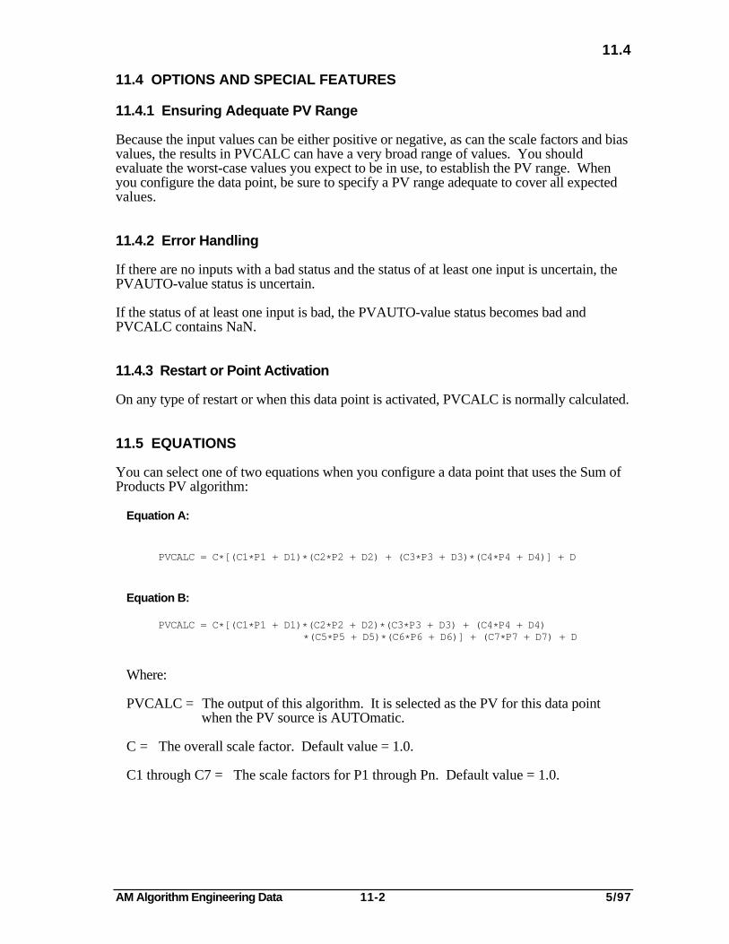
11.5 EQUATIONS
You can select one of two equations when you configure a data point that uses the Sum ofProducts PV algorithm:
Equation A:
PVCALC = C*[(C1*P1 + D1)*(C2*P2 + D2) + (C3*P3 + D3)*(C4*P4 + D4)] + D
Equation B:
PVCALC = C*[(C1*P1 + D1)*(C2*P2 + D2)*(C3*P3 + D3) + (C4*P4 + D4)*(C5*P5 + D5)*(C6*P6 + D6)] + (C7*P7 + D7) + D
Where:
PVCALC = The output of this algorithm. It is selected as the PV for this data pointwhen the PV source is AUTOmatic.
C = The overall scale factor. Default value = 1.0.
C1 through C7 = The scale factors for P1 through Pn. Default value = 1.0.

AM Algorithm Engineering Data 11-3 5/97
11.6
P1 through P7 = The PV input values. Default values are
P1 = NaN.P2 and P3 = 1.0.P4 through P7 = 0.
D = The overall bias. Default value = 0.
D1 through D7 = The bias for P1 through P7. Default value = 0.
Other parameters associated with the SUMPROD algorithm are as follows (refer to theApplication Module Parameter Reference Dictionary):
PnSTS PVEQN
11.6 MIGRATION
There are no similar algorithms in SUPERVISORY/TOTAL Systems, nor in PMXSystems.

AM Algorithm Engineering Data 11-4 5/97

AM Algorithm Engineering Data 12-1 5/97
12
VARIABLE DEAD TIME WITH LEAD-LAG COMPENSATION (PV)Section 12
12.1 TYPE AND NAME
PV Algorithm: VDTLL
12.2 FUNCTION
This algorithm provides a calculated PV (PVCALC) in which value changes may bedelayed from the time that the corresponding change occurred in the P1 input. Dynamiclead-lag compensation to the PV can also be provided. Lag compensation is available incombination with the delay or with no delay. The delay time can be fixed or can be variedas the value of an input varies. See Figure 12-1.
P1
P2
PVCALC(Data PointParameter)
VDTLL
Process Input
Variable DeadTime Input
Equation A: One Lead and Two Lag Compensations
Equation B: Fixed Dead Time
Equation C: Variable Dead Time
Equation D: Variable Dead Time with Two Lag Compensations
Figure 12-1 — Functional Diagram, Variable Dead Time with Lead Lag PV Algo 1316
AM Algorithm Engineering Data 12-2 5/97
12.3
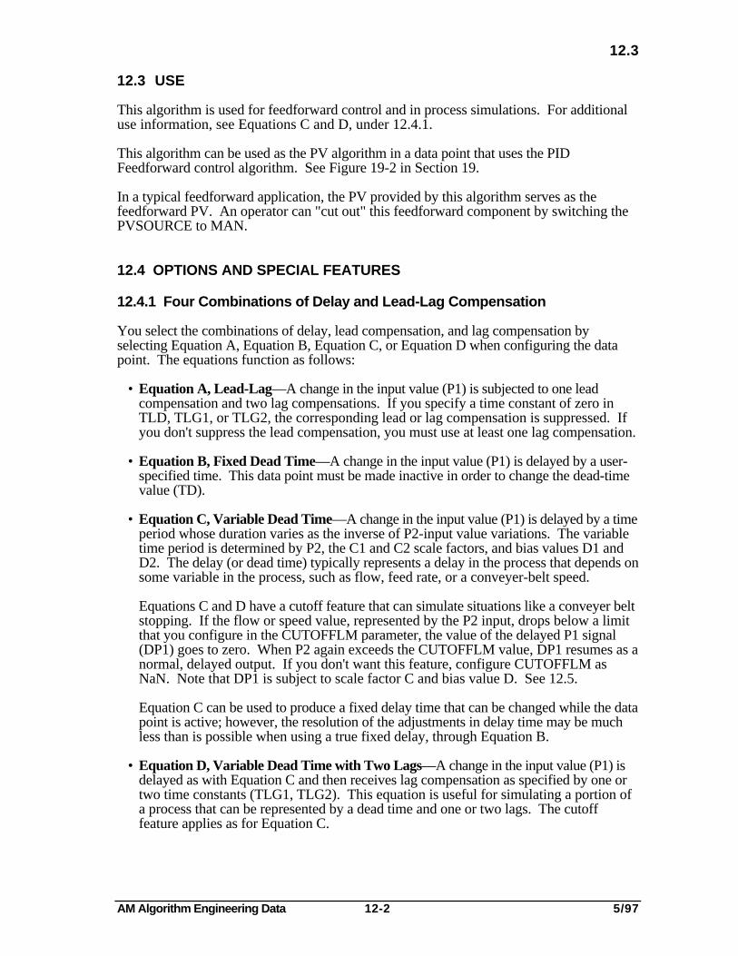
12.3 USE
This algorithm is used for feedforward control and in process simulations. For additionaluse information, see Equations C and D, under 12.4.1.
This algorithm can be used as the PV algorithm in a data point that uses the PIDFeedforward control algorithm. See Figure 19-2 in Section 19.
In a typical feedforward application, the PV provided by this algorithm serves as thefeedforward PV. An operator can "cut out" this feedforward component by switching thePVSOURCE to MAN.
12.4 OPTIONS AND SPECIAL FEATURES
12.4.1 Four Combinations of Delay and Lead-Lag Compensation
You select the combinations of delay, lead compensation, and lag compensation byselecting Equation A, Equation B, Equation C, or Equation D when configuring the datapoint. The equations function as follows:
• Equation A, Lead-Lag—A change in the input value (P1) is subjected to one leadcompensation and two lag compensations. If you specify a time constant of zero inTLD, TLG1, or TLG2, the corresponding lead or lag compensation is suppressed. Ifyou don't suppress the lead compensation, you must use at least one lag compensation.
• Equation B, Fixed Dead Time—A change in the input value (P1) is delayed by a user-specified time. This data point must be made inactive in order to change the dead-timevalue (TD).
• Equation C, Variable Dead Time—A change in the input value (P1) is delayed by a timeperiod whose duration varies as the inverse of P2-input value variations. The variabletime period is determined by P2, the C1 and C2 scale factors, and bias values D1 andD2. The delay (or dead time) typically represents a delay in the process that depends onsome variable in the process, such as flow, feed rate, or a conveyer-belt speed.
Equations C and D have a cutoff feature that can simulate situations like a conveyer beltstopping. If the flow or speed value, represented by the P2 input, drops below a limitthat you configure in the CUTOFFLM parameter, the value of the delayed P1 signal(DP1) goes to zero. When P2 again exceeds the CUTOFFLM value, DP1 resumes as anormal, delayed output. If you don't want this feature, configure CUTOFFLM asNaN. Note that DP1 is subject to scale factor C and bias value D. See 12.5.
Equation C can be used to produce a fixed delay time that can be changed while the datapoint is active; however, the resolution of the adjustments in delay time may be muchless than is possible when using a true fixed delay, through Equation B.
• Equation D, Variable Dead Time with Two Lags—A change in the input value (P1) isdelayed as with Equation C and then receives lag compensation as specified by one ortwo time constants (TLG1, TLG2). This equation is useful for simulating a portion ofa process that can be represented by a dead time and one or two lags. The cutofffeature applies as for Equation C.

AM Algorithm Engineering Data 12-3 5/97
12.4.2
From the process oranother data point
Updated each time the point is processed.
New table input at eachNRATE TS interval
Delayed P1 Output
New interpolated valueeach time the data point
is processed (at each TS interval)
DP1
P1
Maximum of 31 locations
Delay Table
Interpolator
Updated at eachNRATE TS interval.
o o
o*
*
Figure 12-2 — Variable Delay Time Functional Diagram 1317
12.4.2 Dead-Time (Delay-Time) Calculation
The delay of the input values is accomplished by a process that has the effect of shifting thevalues through a table in the module's memory. Values are shifted from one location in thetable to the next, at intervals calculated to provide the desired delay. This is illustrated inFigure 12-2.
For an example of the delay-table operation, suppose that the P1-input value has beenconstant at 5.0 units for an hour. Assume that the specified delay time, TD, is 15 minutesand that the data point is processed every half-minute (TS = 0.5 min.). At this time, theoutput of the interpolator is 5.0 units, all of the locations in the table contain a value of 5.0units, and P1 contains a value of 5.0 units.
Now suppose that the input to P1 suddenly changes to 6.0 units. The interval at whichnew values are shifted through the table and the number of table locations in use have beenset up so that it takes 15 minutes for the new value of 6.0 units to appear at the output ofthe interpolator.
Three sample calculations are provided below. The first shows how a fixed delay time isdetermined (Equation B), the second shows how a variable delay time is determined, andthe third shows how a change in the P2 input changes the variable delay time.
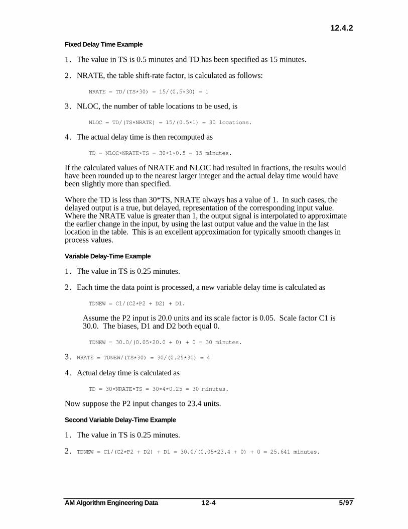
AM Algorithm Engineering Data 12-4 5/97
12.4.2
Fixed Delay Time Example
1. The value in TS is 0.5 minutes and TD has been specified as 15 minutes.
2. NRATE, the table shift-rate factor, is calculated as follows:
NRATE = TD/(TS*30) = 15/(0.5*30) = 1
3. NLOC, the number of table locations to be used, is
NLOC = TD/(TS*NRATE) = 15/(0.5*1) = 30 locations.
4. The actual delay time is then recomputed as
TD = NLOC*NRATE*TS = 30*1*0.5 = 15 minutes.
If the calculated values of NRATE and NLOC had resulted in fractions, the results wouldhave been rounded up to the nearest larger integer and the actual delay time would havebeen slightly more than specified.
Where the TD is less than 30*TS, NRATE always has a value of 1. In such cases, thedelayed output is a true, but delayed, representation of the corresponding input value.Where the NRATE value is greater than 1, the output signal is interpolated to approximatethe earlier change in the input, by using the last output value and the value in the lastlocation in the table. This is an excellent approximation for typically smooth changes inprocess values.
Variable Delay-Time Example
1. The value in TS is 0.25 minutes.
2. Each time the data point is processed, a new variable delay time is calculated as
TDNEW = C1/(C2*P2 + D2) + D1.
Assume the P2 input is 20.0 units and its scale factor is 0.05. Scale factor C1 is30.0. The biases, D1 and D2 both equal 0.
TDNEW = 30.0/(0.05*20.0 + 0) + 0 = 30 minutes.
3. NRATE = TDNEW/(TS*30) = 30/(0.25*30) = 4
4. Actual delay time is calculated as
TD = 30*NRATE*TS = 30*4*0.25 = 30 minutes.
Now suppose the P2 input changes to 23.4 units.
Second Variable Delay-Time Example
1. The value in TS is 0.25 minutes.
2. TDNEW = C1/(C2*P2 + D2) + D1 = 30.0/(0.05*23.4 + 0) + 0 = 25.641 minutes.
AM Algorithm Engineering Data 12-5 5/97
12.4.3
3. NRATE = TDNEW/(TS*30) = 25.641/0.25*30 = 3.419
This is rounded to the nearest integer (not necessarily the next larger integer, as for afixed delay time), so
NRATE = 3.
4. Actual delay time then is
TD = 30*NRATE*TS = 30*3*0.25 = 22.5 minutes.
In the Second Delay Time Example, the exact delay specified by the input was 25.641minutes. If the actual delay is not accurate enough, the TS value can be set lower (byspecifying a lower value for PERIOD) to achieve greater accuracy (resolution).
To eliminate excessive changes and jitter in the TD value that are caused by noise on the P2input, a deadband of 10% of the minimum step in TD values is provided. If P2 doesn'tchange more than this value, the previous TD value is retained.
12.4.3 Changing Dead-Time (Delay-Time) Parameters
Variable delay-time parameters C1, C2, D1, and D2 in Equations C and D can be changedat a Universal Station while the data point is active. Note that the D1 value allows asupervisor or engineer to add a fixed delay time to the total variable delay time.
The C1 and C2 parameters are used to specify the time scale of the P2 value. D1 can beused to offset that scale. Note that the P2 value is inversely proportional to the variabletime delay. Where P2 represents a flow rate or speed, when the flow or speed decreases,the time delay increases to simulate the effect of the reduced flow or speed.
12.4.4 Restrictions on Delay Time
The minimum fixed delay time (Equation B) is equal to TS, the processing interval inminutes. Delay values greater than 32,000*TS are rejected.
For Equations C and D the minimum step-change in the TD value is equal to 30*TS. Thisis also the value of the smallest dead time (delay time). If the TDNEW value is less thanzero, it is clamped to zero. Also, if TDNEW exceeds 32,000*TS, it is clamped to32,000*TS.
12.4.5 Time-Constant Recommendations
We recommend that the processing rate of a data point that uses this algorithm and EquationA or D must be a least ten times greater than the lead or lag break-point frequencies, so,
TLG1 should be equal to or greater than 2*TSTLG2 should be equal to or greater than 2*TS|TLD| should be equal to or greater than 10*TS

AM Algorithm Engineering Data 12-6 5/97
12.4.6
Both positive and negative lead times can be specified, so it is the absolute value of TLDthat must be equal to or greater than 10*TS.
We recommend that the rate amplitude (lag break-point frequency divided by lead break-point frequency) be less than or equal to 10, so,
|TLD| should be equal to or less than 10*TLG1.
12.4.6 Using Equation C or D for a Fixed Delay Time
You can use these variable delay-time equations to attain a fixed delay time by setting thevalue of C1 to 0 and adjusting the value of D1 to get the desired delay value. This permitschanges of delay time from a Universal Station while the data point is active, but theresolution may be much less than using a fixed delay time (Equation B), where the delaycan be changed only by making the point inactive and then active again.
12.4.7 Restart or Point Activation
On a cold start, a warm start, and when the data point is activated, the lead-lag dynamicsare set to the steady state, and all values in the delay table are set to the current value of theP1 input. PVCALC is calculated as follows:
PVCALC = C*P1 +D
On a hot start, all calculations are resumed as if nothing had happened.
12.4.8 Error Handling
For Equation C and D, if neither input has a bad-value status, but one or both has anuncertain-value status, the PVAUTO-value status is uncertain. Equations A and B don'tuse the P2 input, so for them, the PVAUTO-value status is uncertain only if the P1-valuestatus is uncertain.
For Equations C and D, if either input has a bad-value status, PVCALC becomes NaN andthe PVAUTO-value status is bad. For Equations A and B, only a bad P1-value statuscauses PVCALC to contain NaN and the PVAUTO-value status to be bad.
When the input-value status is again normal or uncertain, the data point is initialized as for acold start under 12.4.7, and the PVAUTO-value status becomes normal, or uncertain, asappropriate.
12.5 EQUATIONS
You can select one of four equations when you configure a data point that uses the VariableDead Time with Lead-Lag Compensation PV algorithm:
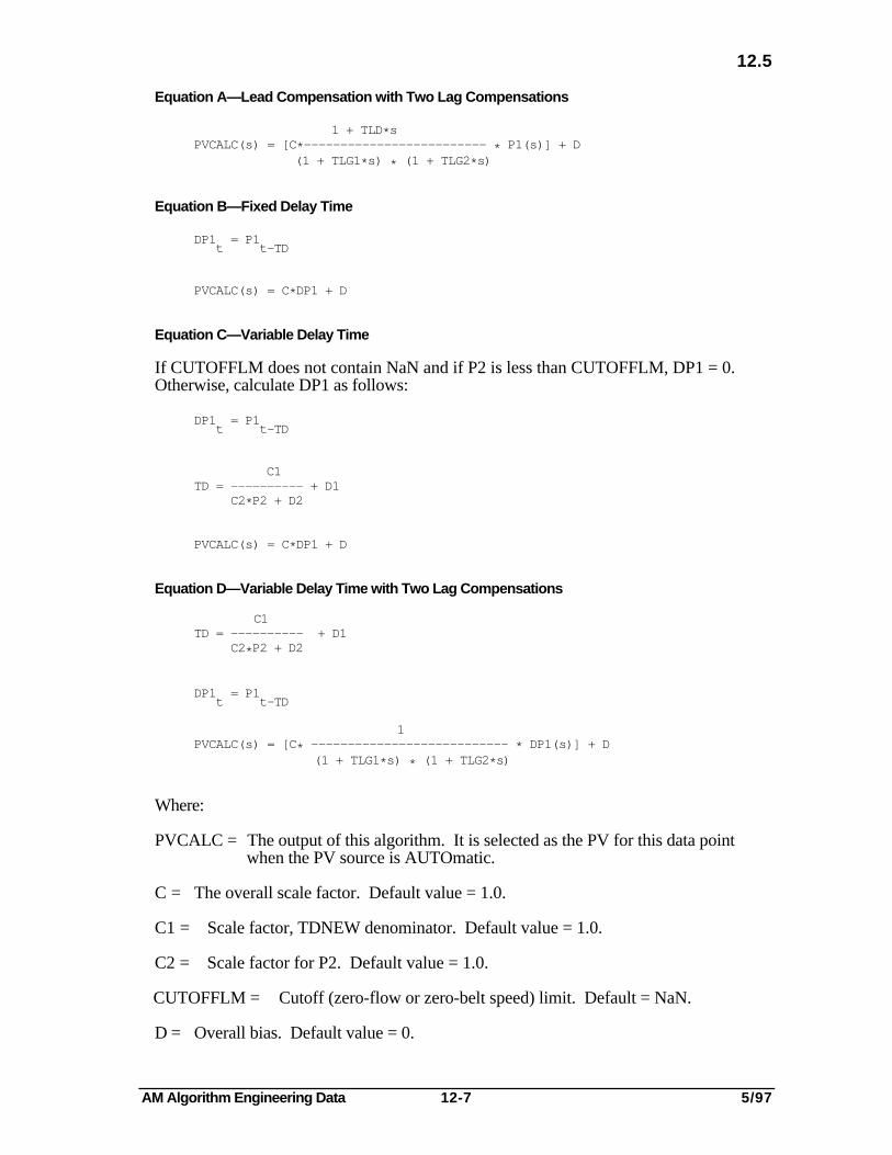
AM Algorithm Engineering Data 12-7 5/97
12.5
Equation A—Lead Compensation with Two Lag Compensations
1 + TLD*sPVCALC(s) = [C*————————————————————————— * P1(s)] + D
(1 + TLG1*s) * (1 + TLG2*s)
Equation B—Fixed Delay Time
DP1t = P1
t-TD
PVCALC(s) = C*DP1 + D
Equation C—Variable Delay Time
If CUTOFFLM does not contain NaN and if P2 is less than CUTOFFLM, DP1 = 0.Otherwise, calculate DP1 as follows:
DP1t = P1
t-TD
C1TD = —————————— + D1 C2*P2 + D2
PVCALC(s) = C*DP1 + D
Equation D—Variable Delay Time with Two Lag Compensations
C1TD = —————————— + D1 C2*P2 + D2
DP1t = P1
t-TD
1PVCALC(s) = [C* ——————————————————————————— * DP1(s)] + D
(1 + TLG1*s) * (1 + TLG2*s)
Where:
PVCALC = The output of this algorithm. It is selected as the PV for this data pointwhen the PV source is AUTOmatic.
C = The overall scale factor. Default value = 1.0.
C1 = Scale factor, TDNEW denominator. Default value = 1.0.
C2 = Scale factor for P2. Default value = 1.0.
CUTOFFLM = Cutoff (zero-flow or zero-belt speed) limit. Default = NaN.
D = Overall bias. Default value = 0.
AM Algorithm Engineering Data 12-8 5/97
12.6
DP1 = The delayed P1 value. Not accessible to Universal Stations nor to user-writtenprograms.
D1 = Bias value for the variable delay time. Default value = 0.
D2 = Bias for P2. Default value = 0.
P1 = The input value to which the delay and lead-lag compensation are applied.
P2 = The input value that changes the variable delay when Equation C or Equation D isused.
s = The Laplace operator (notation only, not a parameter)
t = The present time (notation only, not a parameter)
t-TD = The present time minus the actual dead (delay) time (notation only, not aparameter).
TD = The fixed time delay in minutes for Equation B. The actual variable delay time inminutes for Equations C and D. Default = 0.
TDNEW = The calculated new (ideal) delay time in minutes for Equations C and D.
TLD = Lead-compensation time constant in minutes. 0 = no lead. Default = 0.
TLG1 = Lag-compensation time constant 1 in minutes. 0 = no lag. Default = 0.
TLG2 = Lag-compensation time constant 2 in minutes. 0 = no lag. Default = 0.
Another parameter associated with the VDTLL algorithm is as follows (refer to theApplication Module Parameter Reference Dictionary):
PVEQN
12.6 MIGRATION
The only similar PV algorithms in SUPERVISORY/TOTAL Systems and PMX systemsare delay algorithms 36 and 37. Equations B, C, and D can provide similar fixed delays.The resolution of the calculated delay is significantly better here, because the delay table inthe SUPERVISORY/TOTAL and PMX Systems has a maximum of only 16 locations.
Control algorithm 20 in SUPERVISORY/TOTAL and PMX Systems provides lead-lagcompensation similar to that of Equation A of this algorithm, except that algorithm 20 hasonly one lag-time constant.
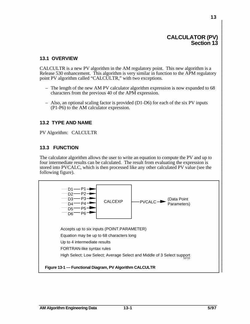
AM Algorithm Engineering Data 13-1 5/97
13
CALCULATOR (PV)Section 13
13.1 OVERVIEW
CALCULTR is a new PV algorithm in the AM regulatory point. This new algorithm is aRelease 530 enhancement. This algorithm is very similar in function to the APM regulatorypoint PV algorithm called “CALCULTR,” with two exceptions.
– The length of the new AM PV calculator algorithm expression is now expanded to 68characters from the previous 40 of the APM expression.
– Also, an optional scaling factor is provided (D1-D6) for each of the six PV inputs(P1-P6) to the AM calculator expression.
13.2 TYPE AND NAME
PV Algorithm: CALCULTR
13.3 FUNCTION
The calculator algorithm allows the user to write an equation to compute the PV and up tofour intermediate results can be calculated. The result from evaluating the expression isstored into PVCALC, which is then processed like any other calculated PV value (see thefollowing figure).
(Data PointParameters)
CALCEXP
Accepts up to six inputs (POINT.PARAMETER)
Equation may be up to 68 characters long
Up to 4 intermediate results
FORTRAN-like syntax rules
High Select; Low Select; Average Select and Middle of 3 Select support
P1P2P3P4P5P6
PVCALC
D1D2D3D4D5D6
16715
Figure 13-1 — Functional Diagram, PV Algorithm CALCULTR
AM Algorithm Engineering Data 13-2 5/97
13.3
The equation is specified at the time of point building and is loaded from the DEB withoutadditional steps such as compilation or linking.
Up to six inputs sources (PISRC(n)) can be configured and stored into the destinationparameters P1 . . . P6.
Up to six scaling factor parameters (D1-D6) are also provided, one for each of the inputdestination parameters, P1 . . . P6.
The following general guidelines apply.
• The equation can be up to 68 characters long.
• FORTRAN-like syntax rules apply.
• Up to 5 levels of nesting of expressions.
• Free format reals and mixed real and integer calculations permitted.
• Up to four intermediate results.
• The result of any expression that has no "equate" associated with it is stored intoPVCALC.
• On point activation or warm restart PVCALC is initialized to the P1 input.
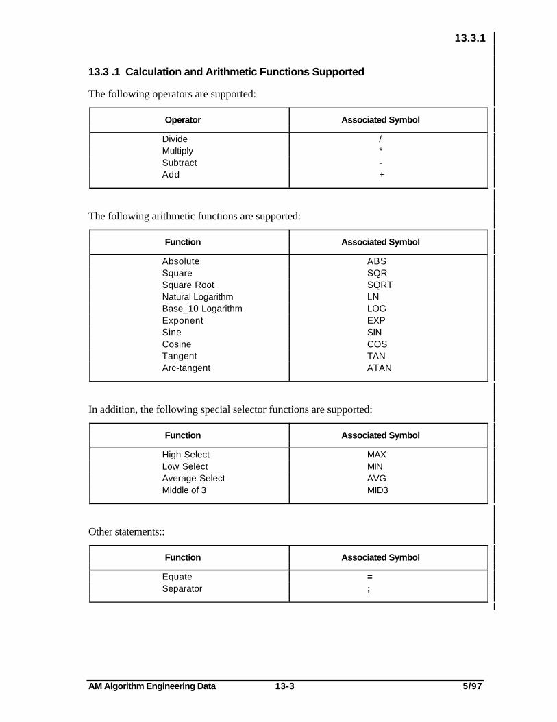
AM Algorithm Engineering Data 13-3 5/97
13.3.1
13.3 .1 Calculation and Arithmetic Functions Supported
The following operators are supported:
Operator Associated Symbol
Divide /Multiply *Subtract -Add +
The following arithmetic functions are supported:
Function Associated Symbol
Absolute ABSSquare SQRSquare Root SQRTNatural Logarithm LNBase_10 Logarithm LOGExponent EXPSine SINCosine COSTangent TANArc-tangent ATAN
In addition, the following special selector functions are supported:
Function Associated Symbol
High Select MAXLow Select MINAverage Select AVGMiddle of 3 MID3
Other statements::
Function Associated Symbol
Equate =Separator ;
AM Algorithm Engineering Data 13-4 5/97
13.4
13.4 USE
The calculator algorithm can be used to perform any calculation or arithmetic function on upto six inputs, using up to four intermediate results.
13.5 OPTIONS AND SPECIAL FEATURES
• The user can configure up to six inputs, using the "Tagname.Parameter" format forPISCRC(n). The destination inputs can be assigned, using PIDSTN(n) for P1 . . . P6.
• Up to four intermediate results can be calculated, for example:
C1=<expr_1>; C2=<expr_2>; C3 =<expr_3>; C4=<expr_4>;<expr_5>
The result of expr_5 is stored in PVCALC (because it has no equate associated with it).There is no restriction on the order in which the sub equations and the expression forPVCALC are specified.
• If C1-C4 are expressions, they are recalculated every time the algorithm is processed.
• If C1-C4 are not expressions, then they can be used as configurable constants into theequation. C1-C4 can then be entered or modified by an operator through the detaildisplays or user programs.
• Parameters D1-D6 are scaling factors for each of the six PV Inputs, P1-P6. The defaultvalue for D1-D6 is 1.0.
13.5.1 Calculator Expression Errors
The calculator expression is compiled during the Data Owner Store into the algorithmexpression string parameter, CALCEXP. In case of any syntax error(s) or if a parameterreferenced in the expression is misspelled, the store is rejected and the error“CALCULATOR SYNTX” is given to the user.
13.5.2 Error Handling of Bad-Inputs and Uncertain Values
If the calculated value of PVCALC is "BAD," PVAUTOST is marked bad. If the final valueof PVCALC is a normal number, PVAUTOST is marked “UNCERTN” if any input that isused in the calculation is uncertain or bad; otherwise it is set equal to NORMAL.
If the HI, LO, and AVG functions have bad inputs, they are ignored in the computation; ifall inputs are bad, the result is marked bad. On MID3 function, if only one input is bad, theresult is set equal to the average of the other two.
AM Algorithm Engineering Data 13-5 5/97
13.6
13.6 EQUATIONS
The calculator equation can be up to 68 characters long. It is entered into the ParameterEntry Display (PED) in the port for the parameter CALCEXP. You can also change theequation from a schematic or User CL program, but the AM Regulatory point must beINACTIVE. You can configure up to four intermediate expressions. The result of anexpression not having an "equate" associated with it is stored in PVCALC.
Examples of use of this algorithm's equation:
(180.0/(.15*P1)) + (P2+P3*LOG(P4))
C1=P1*P2;C2=P4*MAX(0,C1,100);SQRT(C2*10)
MAX (MID3(P1,P2,P3), MID3(P4,P5,P6)
(P1 * P2)/C1

AM Algorithm Engineering Data 13-6 5/97

AM Algorithm Engineering Data 14-1 5/97
14
USER-WRITTEN CL BLOCK (PV)Section 14
14.1 TYPE AND NAME
PV Algorithm: CL
14.2 FUNCTION
This algorithm is a user-written CL block that is like any other CL block except that it isinserted at the PV-algorithm insertion point in the processing sequence (see Figure 2-1) andis executed instead of one of the standard PV algorithms.
The CL block must calculate and store a value in PVCALC. Inputs to the CL block areusually acquired by direct references in CL, but they can also be acquired through generalinputs to a Custom Data Segment (CDS) that is included in the data point. The value placedin PVCALC by the CL block is processed just as PVCALC is processed for any other datapoint that uses a PV algorithm.
PVCALC(Data PointParameter)
CLBlock
Inputsfrom this
and otherdata points
PV Algorithm Processing
Figure 14-1 — Functional Diagram, CL PV Algorithm 1318
14.3 USE
A CL block is used when normal point processing is appropriate but none of the standardPV algorithms will accomplish the desired function. The CL block can be bound to asingle data point if only one point needs its functions or it can be written as a generic CLblock and bound to several data points.
AM Algorithm Engineering Data 14-2 5/97
14.4
Here are two examples of the tasks that should be accomplished by the CL block:
• A Simple Operation—No Storage of Intermediate Values, No Dynamic Calculations
1. Compute the algorithm output value and store it in PVCALC. This setsPVAUTOST to Normal or Bad, based on the value stored.
2. If propagation of uncertain status is needed, check the status of the inputs used forthe calculation to determine the status of the value in PVCALC (Normal, Uncertn,or Bad) and store that status in PVAUTOST.
• An Operation that Includes Storage of Intermediate Values, or Dynamic Calculations, orBoth
1. Compute the value and store it in PVCALC as follows:
If the status of the required input is Bad,
Set PVCALC to NaN (PVAUTO goes Bad automatically)
Else if (PVINIT = On) {*initialization is requested*}
OR (PVAUTO is NaN) {*this is a recovery from a bad PV*}
Compute PVCALC, using the CL block's initialization equation(PVAUTOST is automatically set to Normal).
Else
Compute PVCALC, using the CL block's normal equation.
2. If propagation of uncertain status is needed, check the status of the inputs to beused for the calculation to determine the status of the value to be placed in PVCALC(Normal, Uncertn, or Bad) and store that status in PVAUTOST.
14.4 OPTIONS AND SPECIAL FEATURES
14.4.1 Initialization
No standard initialization is provided. The CL block can monitor the PVINIT parameter todetermine whether to initialize or not.
14.4.2 Restart
The CL block can check the data point's RESTART parameter to determine what type ofrestart, if any, the point is going through, and then take appropriate action.
AM Algorithm Engineering Data 14-3 5/97
14.4.3
14.4.3 Processing Schedule and Execution Time
The CL block should not be used to perform long, complex operations because there maynot be enough time in normal point processing to complete such operations. Points that usea CL PV algorithm should be scheduled at the longest reasonable interval, and should beassigned to the Slow Processor, if possible. If execution of the CL block takes too muchtime, it is aborted and an alarm is generated.
Lengthy, complex operations and calculations should be accomplished by Fortran or Pascalprograms in a CM60.
14.4.4 Parameters Used for Comparisons
The value status of any parameters used for comparisons should be checked before the CLblock does the comparison. A comparison done with a parameter that has a bad valuecauses the CL block to abort.
14.4.5 Error Handling
If a Bad value is used to determine the value to be stored in PVCALC, the PVCALC status,which is indicated by PVAUTOST, must be set to Bad. CLs Allow Bad Value functionmust be used to store a bad value in PVCALC.
14.5 EQUATIONS
The equation(s) used for a CL PV algorithm, if any, is a function of the CL block.
Another parameter associated with the CL PV algorithm is as follows (refer to theApplication Module Parameter Reference Dictionary):
PVINIT
14.6 MIGRATION
PV algorithm 77 in SUPERVISORY/TOTAL and PMX systems has functions that aresimilar to the CL PV algorithm. The following table lists those functions.

AM Algorithm Engineering Data 14-4 5/97
14.6
Table 14-1 — Comparison of SUPERVISORY/TOTAL and PMX Algorithms with CL PV
Function S/T PMX CL PV
Input access Destination words Explicit only General inputs toor explicit Custom Data
Segments orexplicit references.
Accessible Defined list Defined list Same as for all userparameters programs
Enumerations No No Yes
Data type No No Yes. User defineschecking? data types.
Initialization Yes Yes Yes

AM Algorithm Engineering Data 15-1 5/97
15
AUTO MANUAL STATION (CONTROL)Section 15
15.1 TYPE AND NAME
Control algorithm: AUTOMAN
15.2 FUNCTION
In CAScade mode, this algorithm calculates a control output that is equal to the input valueplus a bias value. The bias value is normally provided by a Universal Station operator. InMANual mode, the output is controlled by a Universal Station operator or a user-writtenprogram. See the following figure.
The algorithm is designed to provide "bumpless" returns to cascade operation, if it isconfigured for external initialization, even though its primary data point may not accept theinitialization value from the AUTOMAN data point. When it is configured for internalinitialization, during initialization, the bias value is back-calculated to provide an unchangedoutput when the data point returns to cascade operation.
o
SequenceProgram
or
MANo
o
AUTOMAN CV OP ToSecondary
OutputProcessing
X1oo
From PrimaryData Point
oMAN
INITVALTo
Primary
Equation: CV = X1 + B
CAS
CAS
Figure 15-1 — Functional Diagram, Auto Manual Control Algorithm 1319

AM Algorithm Engineering Data 15-2 5/97
15.3
15.3 USE
The AUTOMAN control algorithm typically serves as the ultimate secondary data point in acascade-control strategy. As such it directly drives the control element (valve) through aPM slot or a Data Hiway-based slot, as shown on the following figure.
This algorithm is very useful for a secondary data point that is one of two or moresecondaries of the same primary data point (a "fan-out" configuration). In such aconfiguration, AUTOMAN can provide a "bumpless" output even if its primary doesn'taccept AUTOMAN's initialization request, but accepts one from one of its othersecondaries. This might happen because the AUTOMAN point is temporarily out of thecascade because it is inactive or because it is in MAN mode.
In a PM, this is an Analog Output point (slot) with PNTFORM = Component. On a Data Hiway this is a CB, MC, or EC point (slot) using a CM, CMA, or DDC algorithm.
AUTOMAN CV OP
OutputProcessing
oMan
oo
To AdditionalSecondaryData Points
CAS
PRIMARYDATA POINT
Note
NOTE:
Figure 15-2 — AUTOMAN Serving as Ultimate Secondary in a Fan-Out Configuration 1320
15.4 OPTIONS AND SPECIAL FEATURES
15.4.1 "Bumpless" Returns to Cascade Operation
To support the use of this algorithm as one of the secondaries in a fan-out configuration,special handling of the bias value is provided. When the data point is configured forexternal initialization, the bias value, B, consists of two components.

AM Algorithm Engineering Data 15-3 5/97
15.4.1
B = B0 + B1
Internal adjustment-value storage. Usually B1 = 0.
Internal storage for operator-entered or program-entered bias value.
When the user or a program enters a bias value in B while in cascade operation, that valuegoes to B0 and B1 is forced to zero. B1 is an internal parameter that cannot be accessed bya user.
When the cascade connection is broken (in MAN mode, initialization-manual input, etc.) avalue is calculated for the primary to initialize to, as follows:
INITVAL = CV - B0
When cascade operation resumes, the value in B1 is calculated as follows:
B1 = INITVAL - OPprim
The actual output value from the primary data point.
If the primary data point did accept AUTOMAN's initialization value, B1 turns out tocontain zero. If the primary did not accept INITVAL, B1 contains a value that causes CVto contain the value it had just before the cascade closed. In either case, CV does not"bump."
If B1 has a value other than zero, that value ramps to zero at a rate specified by the user inthe RATE1 parameter. RATE1 is specified in engineering units-per-second. Thus, whilethe output doesn't "bump" it does ramp to the new value called for by the input from theprimary.
For example, assume that the AUTOMAN data point, configured for external initialization,is operating in CAS mode
X1 = 6
B = 5; B1 = 0, B0 = 5
CV = X1 + B = 11
RATE1 = 2 units per minute
The mode is changed to MANual
INITVAL = CV - B0 = 12 - 5 = 7
The operator changed the output value.
B = 5; B0 = 5, B1 = 5
The primary does initialize
OPprim = 7

AM Algorithm Engineering Data 15-4 5/97
15.4.1
Go back to CAScade mode
X1 = 7
B1 = 7 - 7 = 0
B = B0 + B1 = 5 + 0 = 5
CV = 7 = 5 = 12
Same value as when in MAN mode
Go to MAN mode again
X1 = 9
B1 = INITVAL - OPprim = 7 - 9 = -2
B = 5 - 2 = 3
CV = 9 + 3 = 12
Same as in MAN mode
This time, the primary doesn't accept INITVAL, and the output of the primary went to nineunits
OPprim = 9
Go back to CAScade
X1 = 9
B1 = INITVAL - OPprim = 7 - 9 = -2
B = 5 - 2 = 3
CV = 9 + 3 = 12
Same as in MAN mode
Now, because B1 ramps from -2 units to zero, CV changes as follows:
12 Units
14 Units
1 minute (2 units per minute)

AM Algorithm Engineering Data 15-5 5/97
15.4.2
15.4.2 Operating Modes
This algorithm operates only in MANual or CAScade modes.
15.4.3 Input Value Range
You must configure the X1 input range in XEULO and XEUHI.
15.4.4 Restart or Point Activation
On a cold or warm restart or when the data point is activated, initialization takes place asdescribed under 15.6. On a hot restart, initialization does not occur.
15.4.5 Error Handling
If the X1 input has a bad-value status, the CV value is bad, but the data point remains in thesame mode. When the bad input returns to normal, CV is recalculated and, if configuredfor external initialization, an initialization request is sent to the primary.
15.5 EQUATIONS
This algorithm uses only one equation for normal operation:
CV = X1 + B
Where:
CV = Control-algorithm output in engineering units.
B = Bias value. Default = 0.
X1 = The initializable input.
15.6 INITIALIZATION
You can configure this algorithm for
• No initialization
• Internal initialization
• External initialization
If you choose no initialization, initialization requests are not sent to the primary data pointand any initialization request from a secondary data point is ignored.

AM Algorithm Engineering Data 15-6 5/97
15.7
If you choose internal initialization, when the data point is initialized, the bias value is back-calculated as follows:
B = CV - X1
If you choose external initialization, initialization takes place as described under 15.4.1
15.7 OVERRIDE FEEDBACK PROCESSING
When the data point's secondary uses an Override Selector algorithm (see Figure 15-2), thefollowing functions take place:
• If this point is configured for external initialization and is in CAS mode, OverrideStatus PTORST is returned to this point through special processing. If that status is"not selected," an override-feedback value is calculated as follows, and it is passed onto the AUTOMAN data point's primary:
ORFB = ORFBSEC - B
Feedback value from the secondary
For more detail on override control see Section 23 of this publication, and 3.1.11 in theAM Control Functions manual.
15.8 AUTOMAN PARAMETERS
In addition to the parameters already mentioned, parameter X1STS is associated with theAUTOMAN algorithm (refer to the Application Module Parameter Reference Dictionary).
15.9 MIGRATION
The AUTOMAN algorithm is similar to control algorithm 25 in SUPERVISORY/TOTALand PMX Systems. The equations compare as follows:
AM Terms
CV = X1 + B
S/T-PMX Terms
CN= X + B
In SUPERVISORY/TOTAL and PMX Systems, algorithm 25 operates in AUTO and MANmodes, while the Auto Manual algorithm in Application Modules operates in CAS andMAN modes.
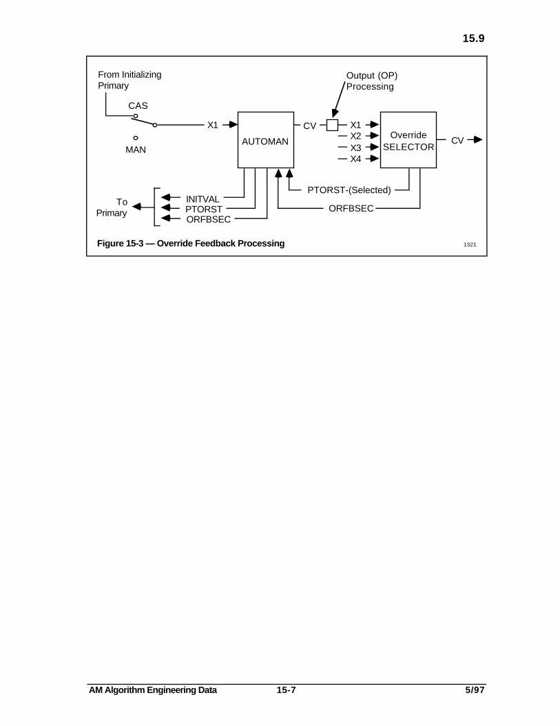
AM Algorithm Engineering Data 15-7 5/97
15.9
oo
AUTOMAN
X1
From InitializingPrimary
CAS
MANo
PTORST-(Selected)
OverrideSELECTOR
ORFBSEC
CV
INITVAL PTORST ORFBSEC
ToPrimary
X1 X2 X3 X4
CV
Output (OP)Processing
Figure 15-3 — Override Feedback Processing 1321

AM Algorithm Engineering Data 15-8 5/97

AM Algorithm Engineering Data 16-1 5/97
16
INCREMENTAL SUMMER (CONTROL)Section 16
16.1 TYPE AND NAME
Control Algorithm: INCRSUM
16.2 FUNCTION
This algorithm calculates the sum of the incremental changes in up-to-four input values.The output is obtained by adding the sum of the changes in all inputs, after each input ismultiplied by a scale factor. See the following figure.
X1X2X3X4
INCRSUM CV OP
OutputProcessing
ToSecondary
X1
X2X3
X4
INCRSUM CV OP
PID
PID
PID
PID
SecondaryData Point
SP
PV
Figure 16-1 — Functional Diagram, Incremental Summer Control Algorithm 1322
16.3 USE
This algorithm is typically used where more than one primary data point is used tomanipulate the setpoint of the same secondary data point. The primaries usually use PIDalgorithms, and are connected to an INCRSUM data point, whose output is connected tothe secondary, as shown here. This is sometimes referred to as a "fan-in connection."
AM Algorithm Engineering Data 16-2 5/97
16.4
16.4 OPTIONS AND SPECIAL FEATURES
16.4.1 Handling of Full Value, Floating PID Outputs
Special handling of the outputs of PID data points is necessary in the Incremental Summer,because it is the dynamic operation of the PID that is significant—the full-value output isnot significant. As the process variables change, PID outputs have no direct relation to theinput, therefore, they are said to be "floating." The incremental summer responds only tochanges in the PID outputs, and calculates a full-value output to be applied to the controldevice (valve) in the process or to the secondary data point.
While the PID algorithms handle SPs, PVs, and outputs as percentages of the configuredrange, the Incremental Summer performs its calculations in engineering units.
To prevent a primary PID point in AUTO or CAS mode from winding-up beyond its ownoutput limits, every time the Incremental Summer point is processed it changes the PID'soutput value to its own CV value after converting to percent. This does not affect thedynamic changes in the PID outputs.
If a primary PID is in MAN mode, the PID's CV is not changed by the IncrementalSummer.
The following restrictions apply to the PID points that are the Incremental Summer point'sprimaries.
• Each must have only one control-output connection.
• Each must reside in the same process unit and the same AM.
• Each must be a normal PID (Section 18) or a PID Feedforward that uses additivefeedforward (Section 19).
16.4.2 Input Value Range
You must configure the X1 input range in XEULO and XEUHI.
16.4.3 Changes to Incremental Summer Output by User-Written Programs
User-written CL programs or user-written programs in a Computing Module can directlystore new values in the CV parameter of the Incremental Summer's data point while theIncremental Summer point is in CAS mode and normally operating. This causes a shift inthe CV value but the dynamic changes continue, because the Incremental Summerdynamically increments or decrements CV each time the point is processed.

AM Algorithm Engineering Data 16-3 5/97
16.4.4
16.4.4 Override Control Strategy and Past-Value Updating
If the Incremental Summer's secondary is an Override Selector data point, the IncrementalSummer's full-value output (CV) must be limited to a user-specified range beyond thefeedback value received from the Selector point when the Incremental Summer is notselected. The feedback value is received in parameter ORFBSEC and you specify theoverrange (or bias) in ORBIAS.
Because the Incremental Summer operates only on changes in value, each time it isprocessed it must store past values. These past values [Xn(n-1)] are used to calculate thechanges in values the next time the Incremental Summer point is processed.
The flow chart of Figure 16-2 shows how the override strategy and past-value updatingoperate. Also see 16.7.
16.4.5 Operating Modes
This algorithm operates only in MANual and CAScade modes. Because the output of eachPID primary tracks the OP output value of the INCRSUM data point, switching this pointfrom MAN to CAS does not "bump" the process.
Note: The dynamic correction calculated by a PID primary appears as a change in that datapoint's output after it is processed again, and the Incremental Summer actually uses thischange as its input. The full-value outputs of PIDs connected to the Incremental Summerhave no meaning.
16.4.6 Restart or Point Activation
On a cold restart, a warm restart, or point activation, if the Incremental Summer isconfigured for initialization, it takes place as described under 16.6. On a hot restart, theinputs and past values become the present values and no initialization requests are sent tothe primary data points.
16.4.7 Error Handing
If the status for an input value is bad, the input value is not used in the CV calculation andthe point remains in the same mode. When a bad input returns to normal, that input isagain used in the CV calculation without "bumping" the value.

AM Algorithm Engineering Data 16-4 5/97
16.4.7
YES
NO
YES
NO
YES
Finishedcalculatingpast valuesfor all inputs
in use?
START
END
CalculateCV
See 15.5
Is secondaryan overrideselector?
Is this datapoint
selected?
NO
NO
YES
CV <(ORFBSEC- ORBIAS)?
CV <(ORFBSEC+ ORBIAS)?
Clamp CV@ ORFBSEC
- ORBIAS
Clamp CV@ ORFBSEC
+ ORBIAS
CV (n - 1)= CV
A
NO
YES
NO
YES
Primary forthis input a
PID?Xn (n - 1)
= XnA
YES
NO, AUTO or CAS
Primary inMAN mode?
Xn (n - 1)= Xn
A
Xn (n - 1) = CV (%)(CV is output ofIncr. Summer)
CV (Primary) = OP(OP is output ofIncr. Summer)
ANOTE: This doesn't necessarily
show algorithm sequencing.It only shows the relationshipof each operation to the next.
Feedback value from Override Selector.
User-entered Override Bias value.
Xn: This input value.Xn (n - 1): Past input value.ORFBSEC:
ORBIAS:
CV (Primary): CV of the primary that provides this input.
Figure 16-2 — Operation Diagram, Incremental Summer Control Algorithm 1323

AM Algorithm Engineering Data 16-5 5/97
16.5
16.5 EQUATIONS
CV is calculated as follows:
CV(n) = CV(n-1) + K1*[X1(n) - X1(n-1)]
+ K2*[X2(n) - X2(n-1)]
.
.
.+ Km*[Xm(n) - Xm(n-1)]
Where:
CV(n) = Current full value of the output of this algorithm in engineering units.
CV(n-1) = Past full value from the data point (value from the last time the data point wasprocessed).
m = The number of inputs actually used (m = 1 through 4).
K1 through Km = User-specified scale factors (gains). K1 default = 1.0. K2 throughK4 default to 0.
X1(n) through Xm(n) = Current values of each X input in use.
X1(n-1) through Xm(n-1) = Past value of each X input (value from the last time thedata point was processed).
16.6 INITIALIZATION
You can configure this algorithm for
• Internal initialization.
• External initialization.
If you choose internal initialization, initialization requests are not sent to any of theprimaries. In MAN mode, when the output is indisposable or when recovering from a badCV value (NaN), initialization is as follows:
CV is back-calculated from OP
if the output is disposable, or
CV = the initialization value returned from the secondary data point, if the output isindisposable.
AM Algorithm Engineering Data 16-6 5/97
16.7
The past values are replaced as follows:
CV(n-1) = CV
X1(n-1) = X1.
.
.
Xm(n-1) = Xm
If you choose external initialization, initialization occurs in MAN mode, when the output isindisposable, or when recovering from a bad CV value (NaN), as follows:
• An initialization request is sent to all primary data points (up to four).
• The Incremental Summer's CV value and past values are initialized as shown above forinternal initialization.
• The initialization value sent to the primary or primaries is equal to the value in theIncremental Summer's CV parameter.
16.7 OVERRIDE FEEDBACK PROCESSING
When this data point's secondary uses an Override Selector algorithm, the IncrementalSummer doesn't send override-selection status nor values to its primaries. It does,however, receive selected or not-selected status from the secondary, and its CV value islimited as described under 14.4.4 and on Figure 14-2.
16.8 INCRSUM PARAMETERS
In addition to the parameters already mentioned, the following parameters are associatedwith the INCRSUM algorithm (refer to the Application Module Parameter ReferenceDictionary):
INITTYPE X3STSX1STS X4STSX2STS
16.9 MIGRATION
There are no similar algorithms in SUPERVISORY/TOTAL and PMX Systems.Algorithm 32, Incremental, in the Extended Controller is similar to the Incremental Summercontrol algorithm.

AM Algorithm Engineering Data 17-1 5/97
17
LEAD-LAG (CONTROL)Section 17
17.1 TYPE AND NAME
Control Algorithm: LEADLAG
17.2 FUNCTION
This algorithm provides dynamic lead and lag compensation to a feedforward signal. Ascale factor can be applied to the input and a bias value can be added.
LEADLAG
CAS
AUTO
SP
From InitializingPrimary
Operator orUser-Written
Program
ToPrimary
ToSecondary
OutputProcessing
CV OP
INITVAL
CV (s) = [K1 + T2 s
1 + T1 s
1
1 + T3 sSP (s) ] + B*
*
**
**
Equation:
Figure 17-1 — Functional Diagram, Lead-Lag Control Algorithm 1324
17.3 USE
This algorithm is used to provide dynamic lead and lag compensation to a feedforwardvariable from a process-connected input or from another data point. The algorithm's outputis often connected to the feedforward input of a PID-with-Feedforward control algorithm.It can also be connected to an input of other types of data points such as an incrementalSummer, a Multiplier/Divider control algorithm, a Summer control algorithm, or an AutoManual Station algorithm.

AM Algorithm Engineering Data 17-2 5/97
17.4
The algorithm can also be used to smooth out changes in the setpoint of another data pointby an operator at a Universal Station.
17.4 OPTIONS AND SPECIAL FEATURES
17.4.1 Operating Modes
This algorithm operates in the following modes:
• AUTO
• MAN
• CAS
17.4.2 Eliminating a Lead or Lag Term
Setting the lead-time constant (T2) to 0, eliminates the contribution of its term from thecompensation. Likewise, a value of 0 for either of the lag-time constants (T1 and T3)eliminates their terms from the compensation.
17.4.3 Time-Constant Recommendations
We recommend that the processing rate of a data point that uses this algorithm be at leastten times greater that the lead or lag break-point frequencies, so
|T2| should be equal to or greater than 10*TS.T1 should be equal to or greater than 2*TS.T3 should be equal to or greater than 2*TS.
Because negative values for lead time are possible, its restrictions are specified in termsof its absolute value (|T2|).
TS is the data-point processing-interval in minutes.
We recommend that the rate amplitude be less than or equal to ten, so
|T2| should be less than or equal to 10*T1.
17.4.4 Restart or Point Activation
On a cold restart, warm restart, or when the point is activated, initialization is performed, asconfigured. No initialization occurs on a hot restart.

AM Algorithm Engineering Data 17-3 5/97
17.4.5
17.4.5 SP Value Range
You must configure the range of the SP value in SPEULO and SPEUHI.
17.5 EQUATIONS
Only one equation is available. It is as follows:
Equation A;
1 + T2*s 1CV(s) = [K*————————*————————*SP(s)] + B
1 + T1*s 1 + T3*s
Where:
CV = Normal control output in engineering units.
B = Bias value. Default value = 0.
K = Scale factor (gain). Default value = 1.0.
SP = Input value (initializable).
s = The Laplace operator.
T2 = Lead-time constant in minutes. Default = 0.
T1= 1st lag-time constant in minutes. Default = 0.
T3 = 2nd lag-time constant in minutes. Default = 0.
17.6 INITIALIZATION
You can configure this algorithm for
• No initialization
• Internal initialization
• External initialization
If no initialization is chosen, normal processing continues if a condition should occur thatwould otherwise cause initialization.
If internal initialization is chosen, an initializing condition causes the bias value (B) to becalculated so that on a return to CAS or AUTO mode the output does not move. Theinitialization equation is
B = CV - K*SP

AM Algorithm Engineering Data 17-4 5/97
17.7
If external initialization is chosen, an initializing condition causes an initialization request tobe sent to the primary, and the value of SP needed to maintain CV at the present value iscalculated and passed to the primary in INITVAL. The initialization equation is
CV - BSP = ———————
K
17.7 OVERRIDE FEEDBACK PROCESSING
This algorithm doesn't participate in override-feedback processing. It should not be usedin an override-control strategy.
17.8 LEADLAG PARAMETERS
In addition to the parameters already mentioned, the following parameters are associatedwith the LEADLAG algorithm (refer to the Application Module Parameter ReferenceDictionary):
INITTYPE SPEUHISPEULO SPSTS
17.9 MIGRATION
Control algorithm 20 in SUPERVISORY/TOTAL and PMX Systems is similar to thisalgorithm, except that algorithm 20 has only one lag term. LEADLAG has normalinitialization options, while algorithm 20 does prevent bumps when the input and outputdon't match, but the output decays toward the steady-state value.
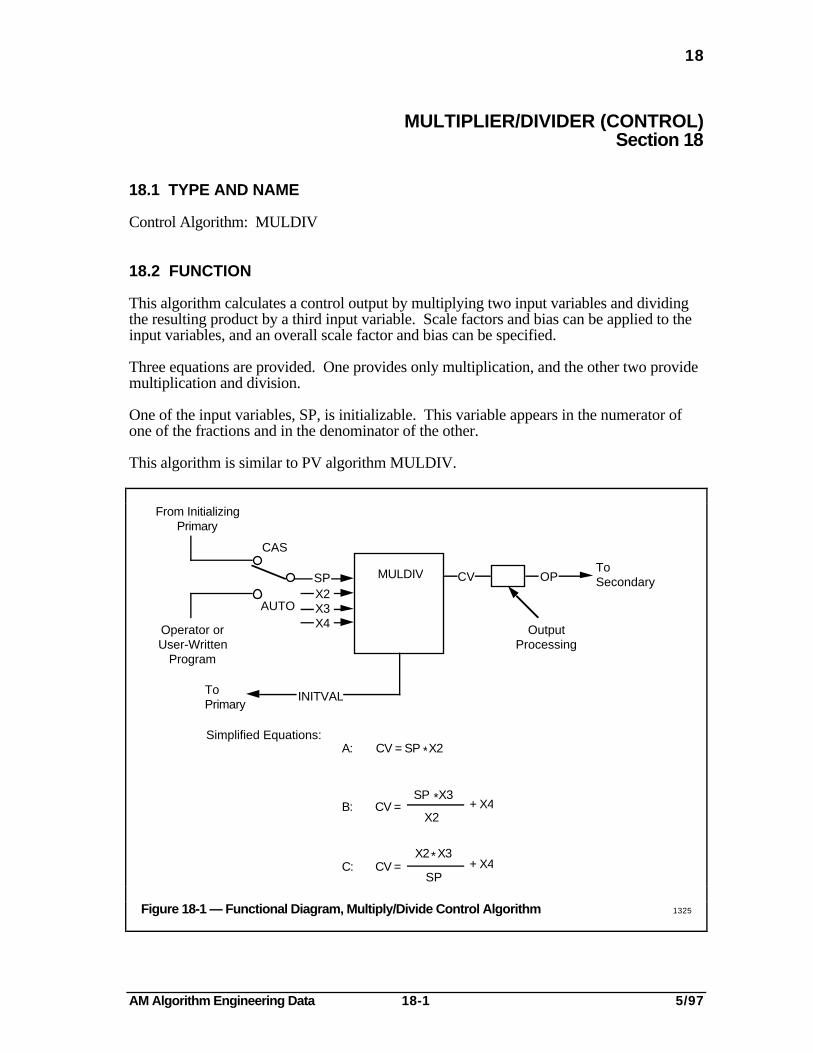
AM Algorithm Engineering Data 18-1 5/97
18
MULTIPLIER/DIVIDER (CONTROL)Section 18
18.1 TYPE AND NAME
Control Algorithm: MULDIV
18.2 FUNCTION
This algorithm calculates a control output by multiplying two input variables and dividingthe resulting product by a third input variable. Scale factors and bias can be applied to theinput variables, and an overall scale factor and bias can be specified.
Three equations are provided. One provides only multiplication, and the other two providemultiplication and division.
One of the input variables, SP, is initializable. This variable appears in the numerator ofone of the fractions and in the denominator of the other.
This algorithm is similar to PV algorithm MULDIV.
MULDIV
CAS
AUTO
SP
From InitializingPrimary
Operator orUser-Written
Program
ToPrimary
ToSecondary
OutputProcessing
CV OP
INITVAL
X2X3X4
Simplified Equations:A: CV = SP X2
B: CV =
C: CV =
SP X3
X2+ X4
X2 X3
SP+ X4
*
*
*
Figure 18-1 — Functional Diagram, Multiply/Divide Control Algorithm 1325

AM Algorithm Engineering Data 18-2 5/97
18.3
Input SP is initializable in all the equations. The only difference between equations B andC is that SP is in the numerator in B and it is in the denominator in equation C.
18.3 USE
This algorithm is normally part of a cascade-control strategy. Typically, its primary is adata point that is using a PID algorithm, and its secondary is another data point that is alsousing a PID algorithm. The Multiply/Divide algorithm can also provide an input to anOverride Selector algorithm.
18.4 OPTIONS AND SPECIAL FEATURES
18.4.1 Operating Modes
This algorithm can operate in the following modes:
• MAN
• AUTO
• CAS
18.4.2 SP Value Range
You must configure the SP-value range in SPEULO and SPEUHI.
18.4.3 Restart or Point Activation
On a cold restart, a warm restart, and then the point is activated, initialization occurs, asconfigured. On a hot restart, no initialization occurs.
18.4.4 Error Handling
When any Xn input is bad, the CV value becomes bad (NaN) and this point continues inthe same mode. When the bad input is again normal, CV is initialized, and if this point isconfigured for external initialization, an initialization request is sent to its primary.
18.5 EQUATIONS
You can select from one of three equations when you build a data point that uses thisalgorithm. The full equations are as follows:
Equation A
CV = [K*(K1*SP+B1)*(K2*X2+B2)] + B
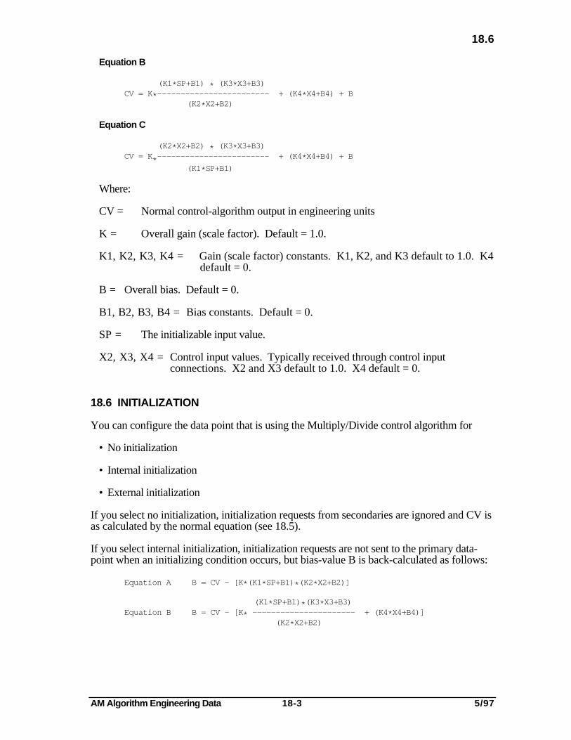
AM Algorithm Engineering Data 18-3 5/97
18.6
Equation B
(K1*SP+B1) * (K3*X3+B3)CV = K*———————————————————————— + (K4*X4+B4) + B
(K2*X2+B2)
Equation C
(K2*X2+B2) * (K3*X3+B3)CV = K*———————————————————————— + (K4*X4+B4) + B
(K1*SP+B1)
Where:
CV = Normal control-algorithm output in engineering units
K = Overall gain (scale factor). Default = 1.0.
K1, K2, K3, K4 = Gain (scale factor) constants. K1, K2, and K3 default to 1.0. K4default = 0.
B = Overall bias. Default = 0.
B1, B2, B3, B4 = Bias constants. Default = 0.
SP = The initializable input value.
X2, X3, X4 = Control input values. Typically received through control inputconnections. X2 and X3 default to 1.0. X4 default = 0.
18.6 INITIALIZATION
You can configure the data point that is using the Multiply/Divide control algorithm for
• No initialization
• Internal initialization
• External initialization
If you select no initialization, initialization requests from secondaries are ignored and CV isas calculated by the normal equation (see 18.5).
If you select internal initialization, initialization requests are not sent to the primary data-point when an initializing condition occurs, but bias-value B is back-calculated as follows:
Equation A B = CV - [K*(K1*SP+B1)*(K2*X2+B2)]
(K1*SP+B1)*(K3*X3+B3)Equation B B = CV - [K* —————————————————————— + (K4*X4+B4)]
(K2*X2+B2)

AM Algorithm Engineering Data 18-4 5/97
18.7
(K2*X2+B2)*(K3*X3+B3)Equation C B = CV - [K* —————————————————————— + (K4*X4+B4)]
(K1*SP+B1)
If you select external initialization, an initializing condition causes INITVAL to becalculated as follows, and that value and an initialization request are sent to the primary datapoint:
(CV - B) 1Equation A INITVAL = [————————————— - B1]*———
K*(K2*X2+B2) K1
(CV - (K4*X4+B4)-B)*(K2*X2+B2) 1Equation B INITVAL = [—————————————————————————————— - B1]*———
K*(K3*X3+B3) K1
K*(K2*X2+B2)-B)*(K3*X3+B3) 1Equation C NITVAL = [——————————————————————————— - B1]*———
CV - (K4+X4+B4) - B K1
18.7 OVERRIDE FEEDBACK PROCESSING
If this data point's secondary is an Override Selector point (see Figure 18-2) and if thispoint is configured for initialization and is in CAS mode, when override-feedbackprocessing takes place, override status and an override value are passed to this point'sprimary. The status is in parameter PTORST. The feedback value is calculated as follows:
Equation A
ORFBSEC - B 1ORFB = [———————————————— - B1]*———
K*(K2*X2 + B2) K1
Equation B
(ORFBSEC - (K4*X4 + B4) - B)*(K2*X2 + B2) 1ORFB = [————————————————————————————————————————— - B1]*———
K*(K3*X3 + B3) K1
Equation C
K*(K2*X2 + B2)*(K3*X3 + B3) 1ORFB = [———————————————————————————— - B1]*———
{ORFBSEC - (K4*X4 + B4) - B} K1
18.8 MULDIV PARAMETERS
In addition to the parameters already mentioned, the following parameters are associatedwith the MULDIV algorithm. Refer to the Application Module Parameter ReferenceDictionary.
CTLEQN SPEUHIINITTYPE SPSTSSPEULO XnSTS

AM Algorithm Engineering Data 18-5 5/97
18.9
18.9 MIGRATION
Table 18-1 compares the AM Multiply/Divide control algorithm with similar algorithms inthe former systems.
MULDIV
CAS
AUTO
SP
From InitializingPrimary
Operator orUser-Written
Program
ToPrimary
CV OPX2X3X4
OverrideSELECTOR
X2X3X4
X1 CV
INITVALPTORST
ORFBSECPTORST
ORFBSEC
Figure 18-2 — Override Feedback Processing 1326
Table 18-1 — Comparison of SUPERVISORY/TOTAL and PMX Algorithms with MULDIV
NearestAM
Equation
S-T/PMXAlgorithmNumber
S-T/PMXEquation inAM Terms
S-T/PMXEquation as shownin S-T/PMX Pubs.
A 31 CV = K*X2*SP + B CN = KA*X*V + K2
B 32 CV = K*SP/X2 + B CN = KA*V/X + K2
A 52 CV = X2*SP + B CN = PV*P + KA
C 53X2
CV = -------- + BSP
PVCN = ------ + KA
P
A 54 CV = SP*X2 + B CN = R*PVN + KA

AM Algorithm Engineering Data 18-6 5/97

AM Algorithm Engineering Data 19-1 5/97
19
PID (CONTROL)Section 19
19.1 TYPE AND NAME
Control Algorithm: PID
19.2 FUNCTION
This algorithm operates as a 3-mode (proportional, integral, and derivative) controller.You can choose one of two forms of this algorithm: the interactive (or real) form and thenoninteractive (or ideal) form.
The output of this algorithm is normally "floating," because of the dynamics of the integraland derivative terms. Internally, the output is calculated as increments of output change,but the increments are accumulated to provide a full-value output, thus simplifying thetechniques used to achieve "bumpless" outputs when modes or tuning constants arechanged.
The algorithm operates to reduce error in the control loop to zero. Error is represented bythe difference between the process variable in percent (PVP) and the setpoint in percent(SPP). The control-algorithm output value (CV) is also calculated as a percentage of theconfigured engineering-units range for the data point that uses this algorithm.
PID
CAS
AUTO
SPP
From InitializingPrimary
Operator orUser-Written
Program
ToSecondary
OutputProcessing
CV OP
SetpointProcessing
From PVProcessing
PVP
PID Forms: Interactive (Real) Noninteractive (Ideal)
Equations: A; Full PIDB; PI on error, D on PV change onlyC; I on error, PD on PV change onlyD; Integral control only
Figure 19-1 — Functional Diagram, PID Control Algorithm 1327

AM Algorithm Engineering Data 19-2 5/97
19.3
19.3 USE
The PID algorithm is used as a controller that either directly moves a control device (valve)in the process, or provides an input to another data point. See the following figure.
DataPoint
In an LCN-based module,in a UPC, or in a box ona Data Hiway.
Or
OPSP
PVPID CV
Output Processing
DirectOutput
SlotNote
Note:
For direct output through a PM, the data point (slot) in the PM is an Analog Output slot whosePNTFORM parameter contains Full and whose RCASOPT parameter = DDC.
For direct output through a CB or MC on a Data Hiway, the data point (slot) in the controller uses one ofthese algorithms in Cas mode (the HG enables the COMP function):
PID CMA (algorithm 05)PID CM (algorithm 06)
For direct output through an EC on a Data Hiway, the data point (slot) in the controller uses one ofthese algorithms in Cas mode (the HG enables the COMP function):
PID DDC (algorithm 05)PID DDC with Preset SP (algorithm 05)Lead/Lag/Summer/DDC (algorithm 06)Selector/Override/DDC (algorithm 21)Lead-Lag/Multiplier/DDC (algorithm 30)
Figure 19-2 — Output Destinations for PID Control Algorithm 3669
When the AM PID point is a primary for another data point in the same AM, another LCNmodule, in a PM, or in a box on a Data Hiway, its output is connected to the SP or thesecondary point. If the AM point is directly controlling a valve, its output is connected tothe output value (OP) of a slot in a PM, or to OP in one of the Data-Hiway-based pointslisted on Figure 19-2. The OP value determines the magnitude of the analog currentsupplied to the valve by the output slot's holding amplifier.

AM Algorithm Engineering Data 19-3 5/97
19.4
19.4 OPTIONS AND SPECIAL FEATURES
19.4.1 Interactive and Noninteractive PID Forms
During configuration, select one of these two forms. They differ as follows:
• Interactive (Real) Form—This form emulates traditional pneumatic-PID controllers.The P, I, and D terms are calculated as the sum of P and I, multiplied by D. D interactsin the time domain with the P and I terms. An advantage of this form is that the poles(lags) and zeros (leads) can be easily placed (See the equations under 19.5). The polesand zeros must be real.
• Noninteractive (Ideal) Form—In this form, P, I, and D are added in the time domain.D is a pure derivative. This form is often called the digital-computer version of the PIDcontroller.
19.4.2 Four Combinations of Control Terms
You select the combinations of proportion, integral, and derivative control terms bychoosing Equation A, B, C, or D. The equations function as follows (also see 19.5):
• Equation A—all three terms (P, I, and D) act on the error (PV - SP).
• Equation B—The proportional and integral terms act on error (PV - SP) and thederivative acts on PV changes. This equation is used to eliminate derivative spikes incontrol action that occur with quick changes in the setpoint.
• Equation C—The integral term acts on error (PV - SP) and the proportion andderivative terms act on PV changes. This equation provides the smoothest and slowestresponse to setpoint changes.
• Equation D—This equation provides only integral control.
19.4.3 Control by a Single Term
When you use equation A, B, or C, the integral or derivative terms can be eliminated bysetting their time constants to 0 (see 19.5). Setting both T1 and T2 to 0 results in onlyproportional control.
Use Equation D to achieve only integral control.
19.4.4 Direct and Reverse Control Action
When configuring a data point that uses the PID algorithm, you can select direct-controlaction or reverse-control action. You can also change the control action through thedetailed display if you have an engineer's key, or a user-written program can change thecontrol action. The control action can be changed at the Universal Station or by a program,only while the data point is in MAN mode. The attribute must be appropriate (OPER orPROG) for the change to be accepted.

AM Algorithm Engineering Data 19-4 5/97
19.4.5
Changing the control action effectively changes the sign of the gain. With direct action, anincrease in PV increases output; with reverse action, an increase in PV decreases output.
As an example, with direct-control action, assume
SPP = 50%
PVP = 51%
Deviation = PVP - SPP = 1%
If PVP increases, the deviation (error) increases, so the output, CV, increases (seeEquation A under 19.5).
The opposite occurs with reverse-control action: If the deviation increases, CV decreases.
19.4.5 PV Tracking
You can select PV tracking when configuring a data point that uses this algorithm. If youdo, SP becomes equal to PV under any of the following conditions:
• The data point that uses this algorithm is in MAN mode.
• The output is indisposable.
• The first time the data point is processed after becoming active.
• On a cold or warm restart, if the data point is configured for external initialization.
• If parameter CTRLINIT contains On and this point is configured for externalinitialization.
PV tracking is typically chosen when the data point is a secondary in a cascade controlstrategy, because it allows the PID to resume control with no error, after the point has beenin MAN mode or is initialized.
PV tracking can also be used when the data point is the ultimate primary point. In such acase, a startup procedure could be used where the point is started in MAN mode and thevalve manually adjusted to bring the PV close to the desired value, and the data point wouldthen be switched to AUTO.
19.4.6 Gain Options
When configuring a data point that uses the PID algorithm, and equations A, B, or C, youcan choose any of the following four gain options:
• Linear Gain—This is the most commonly used gain option. The gain, K, used in thechosen equation (see 19.5) is set by the user. The default value for K is 1.

AM Algorithm Engineering Data 19-5 5/97
19.4.6
• Gap Gain Modification—This option is used to reduce the sensitivity of the controlaction when the PV is in a narrow band (gap) around the setpoint. The size of thisband is specified by the user. K, as used in the chosen equation is derived as follows:
K = KLIN*KGAP, if (SP - GAPLO) < PV < (SP + GAPHI)
or,
K = KLIN, if PV is outside the gap.
Where:
KLIN = A linear-gain parameter, in percent-per-percent. The value of KLIN is tunedat a Universal Station. Default = 1.0.
KGAP = Gain-modification factor, specified by the user. Default = 1.0.
GAPLO = The bottom limit of the gap in the same engineering units as the PV.Default = 0.
GAPHI = The upper limit of the gap in the same engineering units as the PV. Default= 0.
• Nonlinear Gain Modification—This option provides control action proportional to thesquare of the error, rather than the error itself. The gain, K, used by the chosenequation, is derived as follows:
K = KLIN*KNL
KNL = NLFM + (NLGAIN*|PVP - SPP|/100.0)
If the resulting value in K exceeds 120.0, it is clamped at 120.0.
Where:
KLIN = Same as for gap gain
KNL = Nonlinear-gain modifier
NLFM = Nonlinear-gain form. 0 or 1, as specified by the user. Default = 1.
For the ideal form of the PID, nonlinear gain does not act on the derivative component.
NLGAIN = Nonlinear gain, specified by the user. Value ranges from 0 to 10.Default = 0.
PVP = PV in percent
SPP = SP in percent

AM Algorithm Engineering Data 19-6 5/97
19.4.7
• External Gain Modification—The gain, K, used by the chosen equation, is modified byan input value that can be from the process, from a PV calculated from a process inputby a PV algorithm, or from a user-written program.
The main use of this option is to compensate for nonlinear-process gain. The user cantune the PID gain independently of the operating point of the process. For example, incontrolling the level in a tank whose cross section is not constant, the gain could bemodified to compensate for the nonlinear rate of level change that is caused by thechanging shape of the tank. The General Linearization PV algorithm (Section 5) couldbe used to compute the inverse of the level-change characteristic, and the resulting PVcould be used to modify the level-control gain.
K is derived as follows:
K = KLIN*KEXT
If the resulting value in K exceeds 120.0, it is clamped at 120.0.
Where;
KLIN = Same as for linear gain
KEXT = The external gain-modification factor. It can be entered by a user-writtenprogram, or it can be a general input from another data point. KEXT mustbe a positive number.
It is possible to use this option for multiplicative-feedforward control, but the PID withFeedforward-control algorithm (Section 19) is a better choice because it provides abetter operator interface and better recovery from a "bad" feedforward input.
19.4.7 Windup Handling
When the output of this algorithm reaches the user-specified integral or output limits, orreaches the setpoint limits of the data point's secondary, or when a woundup-statusindication is received from the secondary, the PID algorithm stops calculating the integralterm but the calculation of the proportional and derivative terms continues.
This is the same way that windup conditions are handled in Basic Controllers,Multifunction Controllers, and Extended Controllers.
19.4.8 Suppression of Output "Kicks" When Switching to CAS Mode
Without this suppression feature, the first setpoint change after switching from MAN orAUTO to CAS mode could cause a sudden move (kick) in the output because of theproportional or derivative terms. This "kick" occurs when, for some reason, the primarydata point's output is not initialized, and an abrupt change in the setpoint occurs when CASmode resumes.

AM Algorithm Engineering Data 19-7 5/97
19.4.9
To suppress this "kick," the proportional and derivative terms are not calculated the firsttime the PID data point is processed after changing to CAS mode.
This feature is especially useful when the PID point is one of two or more secondaries ofits primary data point. When this data point is changed to CAS mode, even if the primaryis not initialized, the output of this data point does not bump the first time it is processed.
19.4.9 Initializing PID Output without Affecting Dynamics
A user-written program in an Application Module (CL) or a Computing Module (Fortran orPascal) can store a value in the CV parameter of the PID data point, even while thealgorithm is doing its normal, incremental PID calculation. This may change the full-valueoutput of the data point, but it has no effect on the continuing incrementation ordecrementation of the output. It is possible, therefore, for a user-written program toinitialize a PID output without affecting the dynamics of the PID calculations, and withoutinitializing the output of the primary data point.
As an example of the usefulness of this feature, consider a single PID that is controllingtemperature by controlling the flow of either gas or oil. This PID's output is connected toboth flow controllers, but only one connection is active at any time. When a change fromone fuel to the other is made, the user-written program initializes the output of thetemperature-controller PID by storing a new, full-value output in CV. The activeconnection is switched from one to the other, and the dynamic compensation of the flow ofthe new fuel proceeds. The value stored in CV is the setpoint of the new secondary inpercent (SPP). Through this technique, the full-value output of the primary has beeninitialized without initializing its dynamic calculations, so the fuel switchover is quick andsmooth.
19.4.10 Restrictions on Some Values
The following are restrictions on some of the values used with this algorithm:
• The engineering units range that you specify for the PV also applies to the SP.
• For best performance, we recommend that the integral- and derivative-time constants bewithin the following ranges;
20.0*TS < T1 < 20,000*TS
T2 > 100.0*TS for the interactive form of the PID, and
T2 > 10.0*TS for the noninteractive (ideal) form of the PID
Where TS = the interval at which the data point is processed, in minutes.
If the values of T1 or T2 are not within the ranges suggested above, you should adjustthem or TS to bring them within those ranges.

AM Algorithm Engineering Data 19-8 5/97
19.4.11
For the interactive form of the PID, if
T1 < 2.0*TS, and T1 is clamped at 2.0*TS
T2 < 10.0*TS
the respective time constant is treated as 0.
19.4.11 Ratio Control
Ratio control can be achieved by modifying the setpoint input to the PID algorithm by aratio of some other process value, for example, a fuel-to-air ratio in furnace control (it canalso be accomplished with the Ratio Control algorithm. See Section 20). Whenconfiguring a PID data point, you can select one of the following options for modifying thesetpoint:
• No setpoint ratio or bias
• Fixed ratio and bias
• Auto ratio (fixed bias)
• Auto bias (fixed ratio)
If you select one of the ratio and bias options, configured or operator-entered ratio and biasvalues are used to modify the setpoint, by multiplying it by the ratio and adding the biasvalue, only while the data point is in CAS mode. In AUTO mode, the modification doesnot occur because this option is intended to receive the process value to be modified by theratio, only from another data point.
The "Auto" options adjust the ratio or bias while the data point is in AUTO or MANmodes, or is undergoing initialization, so that when it returns to CAS mode, the new SPwon't "bump" the process. The adjustment is as follows:
• For Auto ratio, the operator can change only bias, and ratio is calculated to maintain thesame setpoint when the mode is changed to CAS. The operator can change the ratio inCAS mode.
• For Auto bias, the operator can change only ratio, and bias is calculated to maintain thesame setpoint when the mode is changed to CAS. The operator can change the bias inCAS mode.
Modification of the setpoint by a ratio and a bias is actually handled by setpoint processingrather than by the PID algorithm. It is applied to only PID setpoints.
These options allow this one algorithm to do essentially the same functions as the PIDRatio, PID Auto Ratio, and PID Auto Bias algorithms in Basic Controllers, MultifunctionControllers, and Extended Controllers.
The parameters used for these options are RBOPTION, RATIO, BIAS, RTHILM,RTLOLM, BSHILM, and BSLOLM.

AM Algorithm Engineering Data 19-9 5/97
19.4.12
19.4.12 Operating Modes
The PID algorithm operates in the following modes:
• MAN
• AUTO
• CAS
19.4.13 Restart or Point Activation
On a cold restart, a warm restart, or when the data point is activated, initialization takesplace as described under 19.6. On a hot restart, the PID dynamics are returned to a steadystate.
19.4.14 Error Handling
If the status of the PV value goes bad, the CV value is changed to bad (NaN) and the datapoint remains in the current mode. When the PV-value status returns to normal, the CVvalue is initialized and the PID dynamics are returned to a steady state. If so configured, aninitialization request and initialization value are sent to the primary data point.
19.5 EQUATIONS
You can select one of four equations when you configure a data point that uses the PIDcontrol algorithm. Equations A through D differ in the interactive and noninteractive formsof the algorithm.
For the Interactive form:
Equation A—P, I, and D act on the error
1 + T1*s 1 + T2*sCV(s) = K*[————————*——————————*(PVP(s) - SPP(s))]
T1*s 1 + a*T2*s
Equation B—P and I act on error, D acts on PV
1 + T1*s 1 + T2*s 1 + T1*sCV(s) = K*[—————————*———————————*PVP(s) - —————————*SPP(s)]
T1*s 1 + a*T2*s T1*s
Equation C—I acts on error, P and D act on PV
1 + T1*s 1 + T2*s 1CV(s) = K*[—————————*———————————*PVP(s) - —————*SPP(s)]
T1*s 1 + a*T2*s T1*s
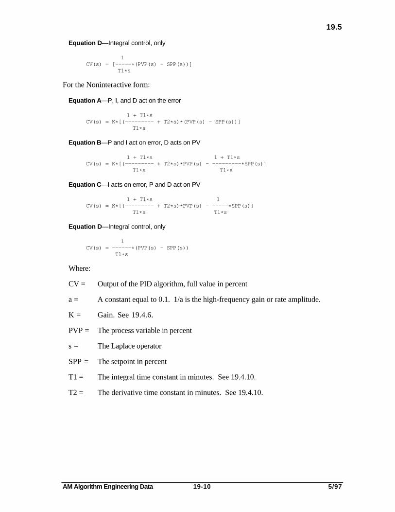
AM Algorithm Engineering Data 19-10 5/97
19.5
Equation D—Integral control, only
1CV(s) = [—————*(PVP(s) - SPP(s))]
T1*s
For the Noninteractive form:
Equation A—P, I, and D act on the error
1 + T1*sCV(s) = K*[(————————— + T2*s)*(PVP(s) - SPP(s))]
T1*s
Equation B—P and I act on error, D acts on PV
1 + T1*s 1 + T1*sCV(s) = K*[(————————— + T2*s)*PVP(s) - —————————*SPP(s)]
T1*s T1*s
Equation C—I acts on error, P and D act on PV
1 + T1*s 1CV(s) = K*[(————————— + T2*s)*PVP(s) - —————*SPP(s)]
T1*s T1*s
Equation D—Integral control, only
1CV(s) = ——————*(PVP(s) - SPP(s))
T1*s
Where:
CV = Output of the PID algorithm, full value in percent
a = A constant equal to 0.1. 1/a is the high-frequency gain or rate amplitude.
K = Gain. See 19.4.6.
PVP = The process variable in percent
s = The Laplace operator
SPP = The setpoint in percent
T1 = The integral time constant in minutes. See 19.4.10.
T2 = The derivative time constant in minutes. See 19.4.10.

AM Algorithm Engineering Data 19-11 5/97
19.6
19.6 INITIALIZATION
You can configure this algorithm for
• Internal initialization
• External initialization
Initialization occurs when the data point is in MAN mode or has just recovered from a badCV, or when the output is indisposable.
If you choose internal initialization, no initialization request or value is sent to the primarydata point. On initialization, if the output is disposable
CV = OP
The output after output processing.
If the output is indisposable, CV is initialized by request from the secondary.
In either case, the PID dynamics are returned to a steady state.
If external initialization is configured
and the mode is MAN, the output is indisposable, or this point has just recovered froma bad CV value,
CV = OP, if the output is disposable
CV is initialized by request from the secondary if the output is indisposable.
If the mode is MAN or AUTO, the output is indisposable, or this point has just recoveredfrom a bad CV value,
an initialization request is sent to the primary. The initialization value sent to theprimary is equal to this data point's setpoint, unless one of the ratio control optionsis chosen. In that case
INITVAL = (SP - BIAS)/RATIO.
19.7 OVERRIDE FEEDBACK PROCESSING
When a PID point's secondary uses an Override Selector algorithm (see Figure 19-3), thefollowing functions take place:
• When override feedback is propagated, override status is returned in PTORST to thePID point. The status will be one of these.
Not Connected
Selected
Not Selected

AM Algorithm Engineering Data 19-12 5/97
19.8
• When the PID point is processed, it does the following.
If the status returned is Not Connected, there is no action.
If the status returned is Not Selected and if the PID point’s mode is AUTO or CAS, thePID point’s CV is initialized in one of two ways. If the direct-control option is chosen,CV is initialized as follows:
CV = (ORFBSEC - CVEULO)/(CVEUHI - CVEULO)*100 + K*(PVP - SPP)
If the reverse-control option is chosen, CV is initialized as follows:
CV = (ORFBSEC - CVEULO)/(CVEUHI - CVEULO)*100 - K*(PVP - SPP)
In both examples above, the term K*(PV - SPP) is the offset value, and ORFBSEC isthe override-feedback value (in %) sent to the PID from the secondary. If equation D isselected for the control algorithm (see 19.5), a value of K = 1.0 is used in theinitialization calculations above (equation D does not use K).
Whether the PID point is selected or not, if it is in CAS mode and configured forexternal initialization, an override-feedback value is calculated as follows and sent to theprimary:
ORFB = (PV - BIAS)/RATIO
The not connected/not selected/selected status received from the PID's secondary, isalso sent on to the primary.
NOTE
For release 410 or later, if the offset value is in such a direction that it causes the nonselectedPID to become selected, the offset value will be set to 0.0. The offset value is the term K*(PV- SPP) in the CV initialization examples above.
See Section 22 in this publication and 3.1.11 in Application Module Control Functions formore information on override control.
19.8 PID PARAMETERS
In addition to the parameters already mentioned, the following parameters are associatedwith the PID algorithm (refer to the Application Module Parameter Reference Dictionary):
CTLEQN INITTYPE PVTRACK DEV

AM Algorithm Engineering Data 19-13 5/97
19.9
19.9 MIGRATION
The PID algorithm virtually duplicates the functions of 9 of the 12 PID algorithms inSUPERVISORY/TOTAL and PMX Systems. Only the interactive (real) form of thealgorithms is available in SUPERVISORY/TOTAL and PMX Systems.
Most of the SUPERVISORY/TOTAL and PMX PID algorithms are actually implementedin Basic Controllers. Four of them can be implemented in the computer system or a BasicController. The following table shows how they compare with the PID in ApplicationModules.
Table 19-1 — Comparison of SUPERVISORY/TOTAL and PMX Algorithms with PID
S/T-PMX Where Nearest AMAlgorithm Implemented? Equivalent
1 PID CB or Computer PID2 PID Ratio CB PID*3 PID Auto Ratio CB PID*4 PID Auto Bias CB PID*5 PID CMA CB PID6 PID CM CB PID7 PID SPC CB PID10 PID Error Sq. on Gain CB or Computer PID11 PID Error Sq. on Intg. CB or Computer PID (See Note)12 PID Gap CB or Computer PID (w/Gap Gain)
* Using Ratio/Bias options in Setpoint Handling.
Note: Error-squared-on-integral gain modification is not available in Application Modules. Nonlinear-gain modification can provide a similar function (see 17.4.6).
Primary
SPP PID
CVAUTO
OP
OverrideSELECTOR
X2X3X4
CAS
From
INITVAL
PTORSTORFBSEC ORFBSEC
ToPrimary
CV
PTORST
ORFBSEC is not an external parameter
X1
Figure 19-3 — Override Feedback Processing 1329

AM Algorithm Engineering Data 19-14 5/97

AM Algorithm Engineering Data 20-1 5/97
20
PID FEEDFORWARD (CONTROL)Section 20
20.1 TYPE AND NAME
Control Algorithm: PIDFF
20.2 FUNCTION
This algorithm operates as a 3-mode (proportional, integral, and derivative) controller. It isidentical to the PID algorithm (Section 19), except that it accepts a feedforward signal to beadded to, or multiplied by, the algorithm's incremental output, before the full-value outputis accumulated. This algorithm lets you combine a feedforward signal with the PID outputwithout using another data point or algorithm to do it.
PIDFF
CAS
AUTO
SPP
From InitializingPrimary
Operator orUser-Written
Program
ToSecondary
OutputProcessing
CV OP
SetpointProcessing
From PVProcessing
PVP
PID Forms: Interactive (Real) Noninteractive (Ideal)
Equations: A; Full PIDB; PI on error, D on PV change onlyC; I on error, PD on PV change onlyD; Integral control only
FeedforwardSignal
Feedforward Action: Additive; Scale and AddMultiplicative; Scale and Multiply
Figure 20-1 — Functional Diagram, PID Feedforward Control Algorithm 1330

AM Algorithm Engineering Data 20-2 5/97
20.3
20.3 USE
The use of the PID Feedforward Control algorithm is the same as the PID algorithm, exceptthat this algorithm can accept a dynamic feedforward signal from the process, or a valuethat is representative of some condition in the process, to be combined with the PID'sincremental output before the full-value output is accumulated.
The feedforward signal can be obtained from an analog-input point, and it is oftensubjected to dead-time compensation, or lead-lag compensation before being connected tothe FF input of this algorithm. That compensation can be provided by algorithms such asthe Variable Dead-Time with Lead-Lag Compensation PV algorithm (Section 12) or theLead-Lag Control algorithm (Section 15). Similar algorithms are available in BasicControllers, Multifunction Controllers, and Extended Controllers. Figure 20-2 shows anexample of such a strategy.
Inlet Feed
FPV Algorithm:
Variable Dead-Timewith Lead-Lag
OutputAccumulation
Auto
Cas
SPP
PVP
PID +, *
%
Dynamic Feed-ForwardSignal
OP
PIDFF Fuel FlowController
FuelT
Outlet Feed
Figure 20-2 — Example, PIDFF Control Algorithm in Head Heater Control 1331
If additive-feedforward action is chosen, the feedforward signal is multiplied by a user-specified scale factor (KF) and added to the incremental output of the PID computation.This scale factor might be used to convert an engineering-units input to a percentage.

AM Algorithm Engineering Data 20-3 5/97
20.4
If multiplicative feedforward action is chosen, the feedforward signal is multiplied by thescale factor (KF) and then multiplied by the incremental output of the PID computation.This action is typically used to compensate for variations in process gain that are caused bychanges in throughput. For example, in a heating application, if the feed rate is doubled,twice the amount of fuel might be required, which is the equivalent of a reduction of one-half in the process gain.
20.4 OPTIONS AND SPECIAL FEATURES
All of the following PID Control-algorithm options and special features apply to the PIDFeedforward Algorithm:
• 19.4.1 Interactive and Noninteractive PID Forms
• 19.4.2 Four Combinations of Control Terms
• 19.4.3 Control By a Single Term
• 19.4.4 Direct and Reverse Control Action
• 19.4.5 PV Tracking
• 19.4.6 Gain Options
• 19.4.7 Windup Handling
• 19.4.8 Suppression of Output "Kicks" when Switching to CAS Mode
• 19.4.9 Initializing PID Output Without Affecting Dynamics, except wheremultiplication of the feedforward signal is configured
• 19.4.10 Restrictions on Some Values
• 19.4.11 Ratio Control
• 19.4.12 Operating Modes; MAN, AUTO, and CAS
• 19.4.13 Restart or Point Activation
• 19.4.14 Error Handling
In addition, the following apply to the feedforward action.
20.4.1 Add or Multiply Action
Parameter FFOPT is configured to specify whether the feedforward signal is to be added tothe incremental PID output or multiplied by it.

AM Algorithm Engineering Data 20-4 5/97
20.4.2
20.4.2 Bypassing Feedforward Control Action
An operator at a Universal Station or a user-written program can bypass the feedforwardaction by one of the following:
• If the feedforward input is received through a control-input connection, change thestatus of that connection to Inactive. To resume feedforward action, switch theconnection status back to Active.
• If the feedforward signal comes from a PV algorithm, switch the PV source for the datapoint that is using the PV algorithm to MANUAL (if you do this and the PV is changedwhile the PV source is in manual, the feedforward signal is affected). To resumefeedforward action, switch the PV source back to AUTO.
• If the feedforward signal comes from a control algorithm, switch the mode of the datapoint that is using the control algorithm to MANual (if you do this and the output (OP)is changed while the source point is in manual, the feedforward signal is affected). Toresume feedforward action, switch back to Normal mode (AUTO or CAS).
20.4.3 Feedforward Signal Value Status
If the value status for the feedforward signal goes bad, the feedforward component of theoutput value is frozen at the last good value, and normal PID processing continues.
When the value status of the feedforward signal returns to normal, normal feedforwardaction resumes. This does not cause a bump in the output because any change from the lastgood value is internally absorbed and the PID dynamics are not affected. The floating, full-value output continues as if there were no feedforward change, but the contribution of thefeedforward action continues from that time.
20.5 EQUATIONS
You can select PID equations, just as described for the interactive form and thenoninteractive form under 19.5.
In addition, the feedforward signal is applied to the incremental output of the PIDcomputation, as follows:
• If additive action is configured
CVn = CVn+1 + CVPID + KFF*(FFn - FFn-1)
If the status of FFn or FFn-1 is Bad, CV = CVPID.
• If multiplicative action is configured
CVn = (CVn-1 + CVPID)*(KFF*FFn + BFF)
When multiplicative action is configured, CV is a read-only parameter for CLprograms.

AM Algorithm Engineering Data 20-5 5/97
20.6
If the status of FFn is Bad, CV = CVPID*(KFF*FF lgv + BFF),where FF lgv = last good value of FF.
If FFn is OK but the status of FFn-1 is bad, CVPID = CV/(KFF*FFn + BFF).
Note that the back calculation of CVPID keeps CV unchanged, and thus, prevents abump.
If the result of (KFF*FFn + BFF) is less than 0.1, it is clamped at 0.1.
Where:
CV = Full-value output in percent, PID combined with feedforward action.
CVPID = The incremental output of the PID computation. This is an internalparameter and is not available to displays nor to user-written programs.
BFF = Bias value for multiplicative action. Default = 0.
FF = The feedforward input signal, from a control-input connection. Normallyfrom a parameter with a percentage value.
FF lgv = Last good value for the FF input (notation only, not a user-visibleparameter).
KFF = Scale factor. Can be used to convert FF to percent as follows;
KFF = 100/(EUHI - EULO)
Where EUHI and EULO are the high and low limits of the engineering-unitsrange. Default = 1.0.
n and n-1 = Notation to indicate the value this pass (n) and the preceding pass (n-1).
20.6 INITIALIZATION
Initialization is as described under 19.6
AM Algorithm Engineering Data 20-6 5/97
20.7
20.7 OVERRIDE FEEDBACK PROCESSING
Override-feedback processing is the same as described under 19.7, except that, ifmultiplicative action is configured, a feedforward term is added to the output calculation, asfollows:
If the status returned is not selected and if the PID point's mode is AUTO or CAS, thePID point's CV is initialized as follows:
CV = (ORFBSEC - CVEULO)/(CVEUHI - CVEULO)*100 + K*(KFF*FF +BFF)*(PVP - SPP)
if the direct-control option is chosen, or
CV = (ORFBSEC - CVEULO)/(CVEUHI - CVEULO)*100 - K*(KFF*FF +BFF)*(PVP - SPP)
if the reverse-control option is chosen.
ORFBSEC is the override-feedback value from the secondary.
20.8 PIDFF PARAMETERS
In addition to the parameters already mentioned, parameter FFSTS is associated with thePIDFF algorithm. Refer to the Application Module Parameter Reference Dictionary.
20.9 MIGRATION
No PID algorithms that combine a feedforward signal with the PID output are available inSUPERVISORY/TOTAL or PMX Systems. See 19.8.

AM Algorithm Engineering Data 21-1 5/97
21
PID WITH EXTERNAL RESET-FEEDBACK (CONTROL)Section 21
21.1 TYPE AND NAME
Control Algorithm: PIDERFB
21.2 FUNCTION
This algorithm operates as a 3-mode (proportional, integral, and derivative) controller. It isidentical to the PID algorithm (Section 18), except that it accepts a reset feedback signal tobe combined with this algorithm's incremental output, before the full-value output isaccumulated. It also accepts a tracking-value signal.
The intent of this algorithm is to prevent windup when it has a secondary data point,typically a PID point, that may or may not be responding to the output of this data point.
PIDERFB
CAS
AUTO
SPP
From InitializingPrimary
Operator orUser-Written
Program
ToSecondaryCV OP
SetpointProcessing
From PVProcessing
PVP
PID Forms: Interactive (Real) Noninteractive (Ideal)
Equations: A; Full PIDB; PI on error, D on PV change onlyC; I on error, PD on PV change onlyD; Integral control only
Reset Feedforward Action: Scaled, integrated CV - RFB deviation is added to incremental PID output before full-value output accumulation.
Tracking Switch ControlTracking Value*Reset Feedback Value**
S1TRFBRFB
*
**
Typically PV or SP ofSecondary PID
Typically PV ofSecondary PID
OutputProcessing
Figure 21-1 — Function Diagram, PID with External Feedback Control Algorithm 1332
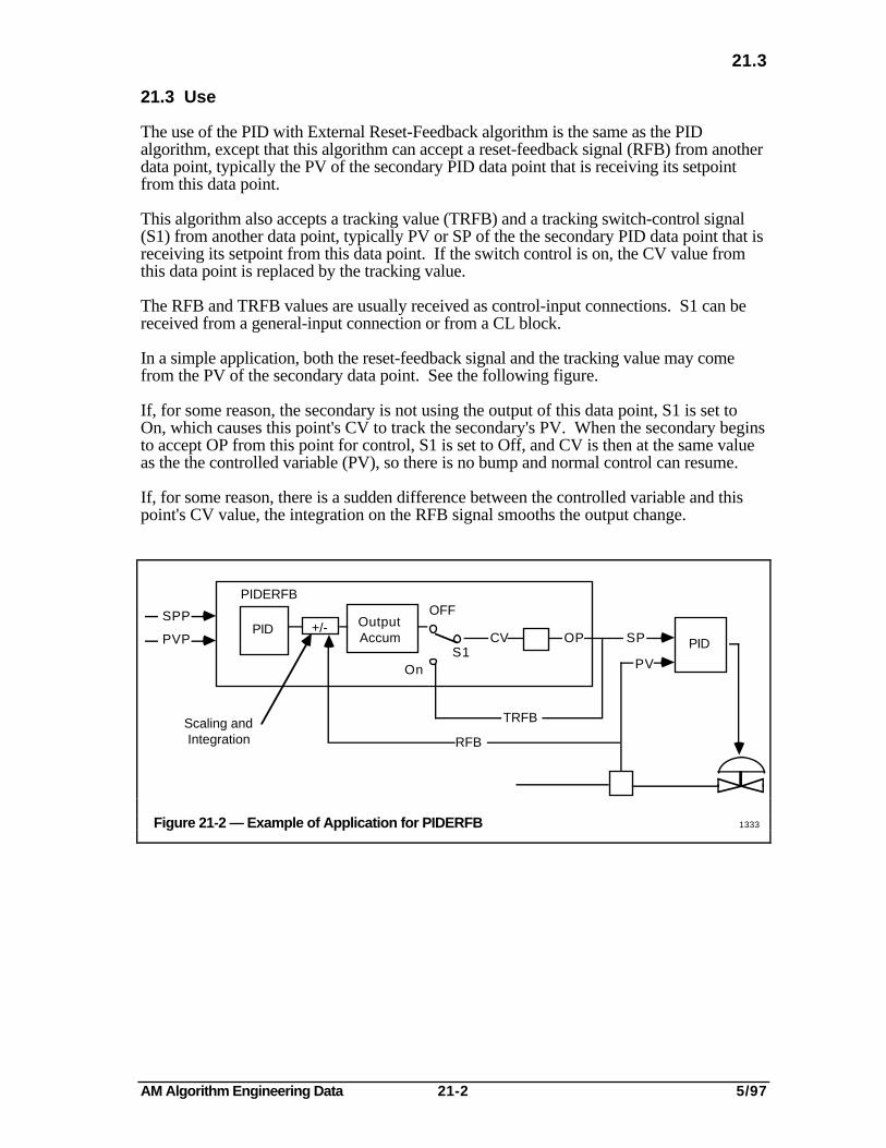
AM Algorithm Engineering Data 21-2 5/97
21.3
21.3 Use
The use of the PID with External Reset-Feedback algorithm is the same as the PIDalgorithm, except that this algorithm can accept a reset-feedback signal (RFB) from anotherdata point, typically the PV of the secondary PID data point that is receiving its setpointfrom this data point.
This algorithm also accepts a tracking value (TRFB) and a tracking switch-control signal(S1) from another data point, typically PV or SP of the the secondary PID data point that isreceiving its setpoint from this data point. If the switch control is on, the CV value fromthis data point is replaced by the tracking value.
The RFB and TRFB values are usually received as control-input connections. S1 can bereceived from a general-input connection or from a CL block.
In a simple application, both the reset-feedback signal and the tracking value may comefrom the PV of the secondary data point. See the following figure.
If, for some reason, the secondary is not using the output of this data point, S1 is set toOn, which causes this point's CV to track the secondary's PV. When the secondary beginsto accept OP from this point for control, S1 is set to Off, and CV is then at the same valueas the the controlled variable (PV), so there is no bump and normal control can resume.
If, for some reason, there is a sudden difference between the controlled variable and thispoint's CV value, the integration on the RFB signal smooths the output change.
SPP
PVP
PIDERFB
PID OutputAccum CV
OnS1
SP
PV
+/-
RFB
TRFB
PID
OFF
Scaling and Integration
OP
Figure 21-2 — Example of Application for PIDERFB 1333
AM Algorithm Engineering Data 21-3 5/97
21.4
21.4 OPTIONS AND SPECIAL FEATURES
All of the following PID Control-algorithm options and special features apply to the PIDwith External Reset Feedback algorithm:
• 18.4.1 Interactive and Noninteractive PID Forms
• 18.4.2 Four Combinations of Control Terms
• 18.4.3 Control By a Single Term
• 18.4.4 Direct and Reverse Control Action
• 18.4.5 PV Tracking
• 18.4.6 Gain Options
• 18.4.7 Windup Handling
• 18.4.8 Suppression of Output "Kicks" when Switching to CAS Mode
• 18.4.9 Initializing PID Output Without Affecting Dynamics
• 18.4.10 Restrictions on Some Values
• 18.4.11 Ratio Control
• 18.4.12 Operating Modes; MAN, AUTO, and CAS
• 18.4.13 Restart or Point Activation
• 18.4.14 Error Handling
In addition, the following applies to the PID with External Reset Feedback.
21.4.1 Error Handling, RFB and TRFB Inputs
If S1 is Off, and the reset-feedback input has a bad value, the data-point mode doesn'tchange and the CV value goes bad (NaN). When the RFB input is again good, the CVvalue is initialized (see 18.6) and the dynamic terms are returned to a steady state. Ifconfigured for external initialization, an initialization request is sent to the primary datapoint.
If S1 is On, and the tracking-value input has a bad value, the data-point mode doesn'tchange and the CV value goes bad (NaN). When the TRFB input is again good, the CVvalue is initialized (see 18.6) and the dynamic terms are returned to a steady state. If soconfigured, an initialization request is sent to the primary data point.
21.4.2 Control Output Connections
Control output connections cannot be configured for this algorithm.
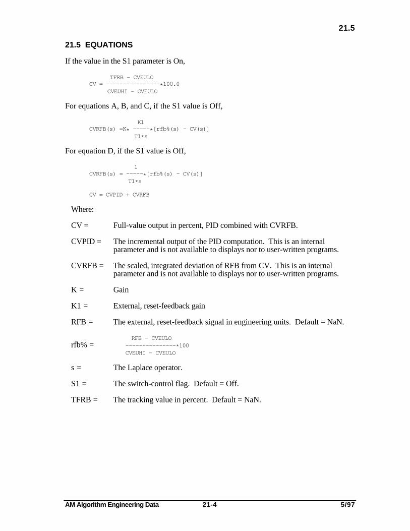
AM Algorithm Engineering Data 21-4 5/97
21.5
21.5 EQUATIONS
If the value in the S1 parameter is On,
TFRB - CVEULOCV = ————————————————*100.0
CVEUHI - CVEULO
For equations A, B, and C, if the S1 value is Off,
K1CVRFB(s) =K* —————*[rfb%(s) - CV(s)]
T1*s
For equation D, if the S1 value is Off,
1CVRFB(s) = —————*[rfb%(s) - CV(s)]
T1*s
CV = CVPID + CVRFB
Where:
CV = Full-value output in percent, PID combined with CVRFB.
CVPID = The incremental output of the PID computation. This is an internalparameter and is not available to displays nor to user-written programs.
CVRFB = The scaled, integrated deviation of RFB from CV. This is an internalparameter and is not available to displays nor to user-written programs.
K = Gain
K1 = External, reset-feedback gain
RFB = The external, reset-feedback signal in engineering units. Default = NaN.
RFB - CVEULOrfb% = ———————————————*100
CVEUHI - CVEULO
s = The Laplace operator.
S1 = The switch-control flag. Default = Off.
TFRB = The tracking value in percent. Default = NaN.

AM Algorithm Engineering Data 21-5 5/97
21.6
21.6 INITIALIZATION
Initialization is as described under 18.6.
21.7 OVERRIDE FEEDBACK PROCESSING
Override-feedback processing is as described under 18.7; however, use of PIDERFB inoverride strategies is not recommended.
21.8 PIDERFB PARAMETERS
In addition to the parameters already mentioned, the following parameters are associatedwith the PIDERFB algorithm. Refer to the Application Module Parameter ReferenceDictionary:
RFBSTS TRFBSTS
21.9 MIGRATION
There is no similar algorithm in SUPERVISORY/TOTAL Systems nor in PMX Systems.There is a similar algorithm, no. 13, in Extended Controllers.

AM Algorithm Engineering Data 21-6 5/97

AM Algorithm Engineering Data 22-1 5/97
22
RATIO (CONTROL)Section 22
22.1 TYPE AND NAME
Control Algorithm: RATIOCTL
22.2 FUNCTION
This algorithm calculates a setpoint, for a PID algorithm, that is the desired ratio of acontrolled variable to an uncontrolled variable. The value of the controlled variable ismaintained at a specified ratio of the value of the uncontrolled variable. The data point thatuses this algorithm usually uses Equation B of the Multiplier/Divider PV algorithm (Section9) to calculate the measured value of the ratio for displays and reports.
Ratio control can also be accomplished with the ratio-control options of the PID or PIDFeedforward control algorithms (see 18.4.11). This Ratio-control algorithm, has severaladvantages, including the display of the actual ratio attained, as calculated by theMultiplier/Divider PV algorithm, and direct control of the ratio through the SP of the Ratioalgorithm.
CAS
X2
PVFrom Initializing
Primary
Operator orUser-Written
Program
AUTO
SP RATIOCTL CV OP To Secondary(Typically, SPfor a PID)
OutputProcessing
UncontrolledVariable
Value Necessary to Maintain the Ratio
Actual Ratio fromPV Calculator Algo
Figure 22-1 — Functional Diagram, Ratio Control Algorithm 1334
22.3 USE
This algorithm is typically used in the control of the flow of a gas or fluid, as a ratio of anuncontrolled or "wild" flow. For example, in a furnace, the air supply might be controlledas a ratio of the fuel supply. If more heat is required to maintain combustion efficiency, thefuel flow is increased and the air flow can be increased as a ratio of the fuel-flow increase.
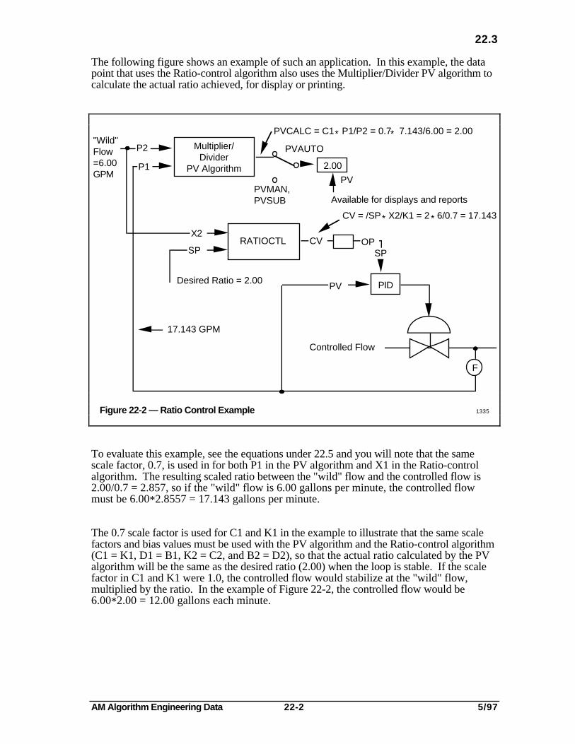
AM Algorithm Engineering Data 22-2 5/97
22.3
The following figure shows an example of such an application. In this example, the datapoint that uses the Ratio-control algorithm also uses the Multiplier/Divider PV algorithm tocalculate the actual ratio achieved, for display or printing.
PVCALC = C1 P1/P2 = 0.7 7.143/6.00 = 2.00
2.00
PV
PVAUTO
PVMAN,PVSUB Available for displays and reports
P2
P1
RATIOCTL
CV = /SP X2/K1 = 2 6/0.7 = 17.143
PID
Multiplier/Divider
PV Algorithm
F
Controlled Flow
Desired Ratio = 2.00
17.143 GPM
CV OPSP
PV
SP
X2
"Wild"Flow=6.00GPM
*
* *
*
Figure 22-2 — Ratio Control Example 1335
To evaluate this example, see the equations under 22.5 and you will note that the samescale factor, 0.7, is used in for both P1 in the PV algorithm and X1 in the Ratio-controlalgorithm. The resulting scaled ratio between the "wild" flow and the controlled flow is2.00/0.7 = 2.857, so if the "wild" flow is 6.00 gallons per minute, the controlled flowmust be 6.00*2.8557 = 17.143 gallons per minute.
The 0.7 scale factor is used for C1 and K1 in the example to illustrate that the same scalefactors and bias values must be used with the PV algorithm and the Ratio-control algorithm(C1 = K1, D1 = B1, K2 = C2, and B2 = D2), so that the actual ratio calculated by the PValgorithm will be the same as the desired ratio (2.00) when the loop is stable. If the scalefactor in C1 and K1 were 1.0, the controlled flow would stabilize at the "wild" flow,multiplied by the ratio. In the example of Figure 22-2, the controlled flow would be6.00*2.00 = 12.00 gallons each minute.

AM Algorithm Engineering Data 22-3 5/97
22.4
Note that the "wild" flow might not be wild at all, but may actually be a flow controlled byanother controller. In any case, the controlled flow stabilizes at a value equal to the "wild"flow, multiplied by the desired ratio, as modified by any scale factors other than 1.0 or anybias values other than 0.
22.4 OPTIONS AND SPECIAL FEATURES
22.4.1 Role of the Multiplier/Divider PV Algorithm
Any data point that uses RATIOCTL should use the Multiplier/Divider PV algorithm(Section 9). Equation B of the Multiplier/Divider algorithm can be used. The uncontrolled("wild") variable is connected to P2 and the variable controlled by the PID algorithm (seeFigure 22-2) is connected to P1. The scale factors and bias values in the PV algorithmmust have the same values as their counterparts in the Ratio control algorithm:
RATIOCTL MULDIV
K1 = C1K2 = C2B1 = D1B2 = D2
Thus, MULDIV can calculate the actual (measured) ratio attained, and when the PV sourceis AUTO, that value is available in the PV parameter of the data point for use on displaysand reports.
22.4.2 Operating Mode
The RATIOCTL algorithm operates in the following modes:
• MAN
• AUTO
• CAS
22.4.3 Restart or Point Activation
On a cold or warm restart or when the RATIOCTL data point is activated, initializationtakes place as described under 22.6. On a hot restart, normal operation resumes with noinitialization.
22.4.4 Error Handling
If the value status of the X2 input is bad, the CV value is changed to bad (NaN). The datapoint remains in the same mode. When the X2 input again has normal status, initializationtakes place as described under 22.6.
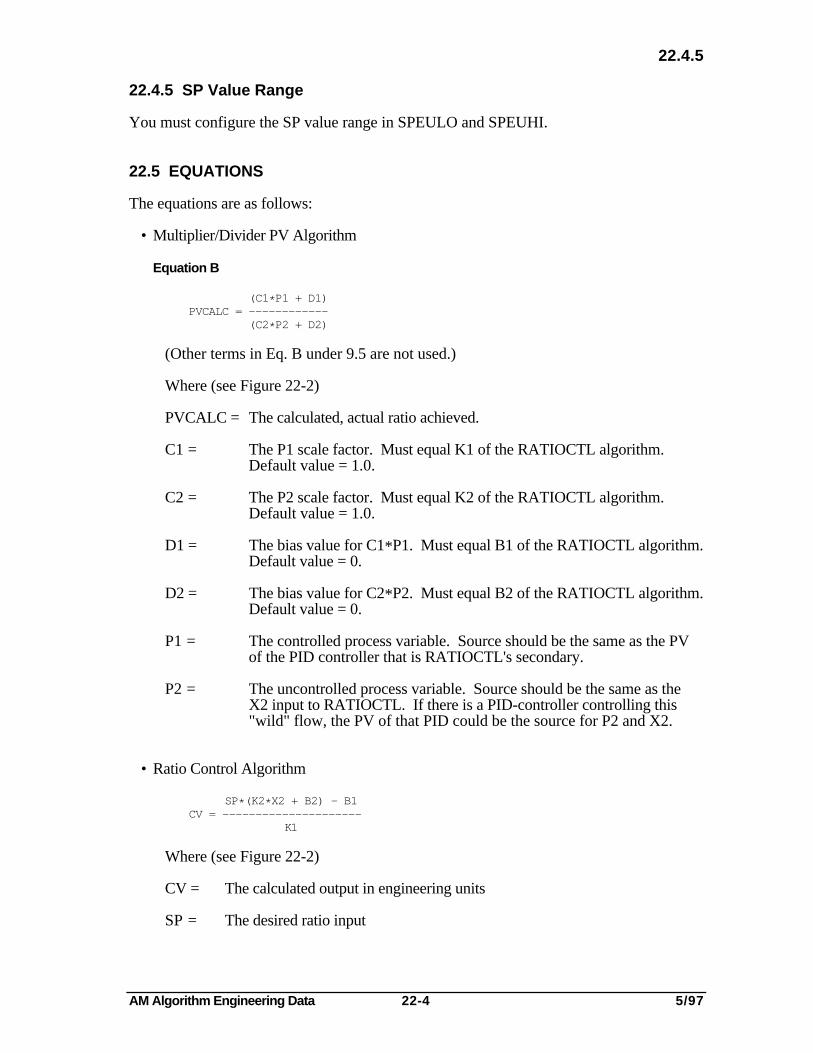
AM Algorithm Engineering Data 22-4 5/97
22.4.5
22.4.5 SP Value Range
You must configure the SP value range in SPEULO and SPEUHI.
22.5 EQUATIONS
The equations are as follows:
• Multiplier/Divider PV Algorithm
Equation B
(C1*P1 + D1)PVCALC = ————————————
(C2*P2 + D2)
(Other terms in Eq. B under 9.5 are not used.)
Where (see Figure 22-2)
PVCALC = The calculated, actual ratio achieved.
C1 = The P1 scale factor. Must equal K1 of the RATIOCTL algorithm.Default value = 1.0.
C2 = The P2 scale factor. Must equal K2 of the RATIOCTL algorithm.Default value = 1.0.
D1 = The bias value for C1*P1. Must equal B1 of the RATIOCTL algorithm.Default value = 0.
D2 = The bias value for C2*P2. Must equal B2 of the RATIOCTL algorithm.Default value = 0.
P1 = The controlled process variable. Source should be the same as the PVof the PID controller that is RATIOCTL's secondary.
P2 = The uncontrolled process variable. Source should be the same as theX2 input to RATIOCTL. If there is a PID-controller controlling this"wild" flow, the PV of that PID could be the source for P2 and X2.
• Ratio Control Algorithm
SP*(K2*X2 + B2) - B1CV = —————————————————————
K1
Where (see Figure 22-2)
CV = The calculated output in engineering units
SP = The desired ratio input
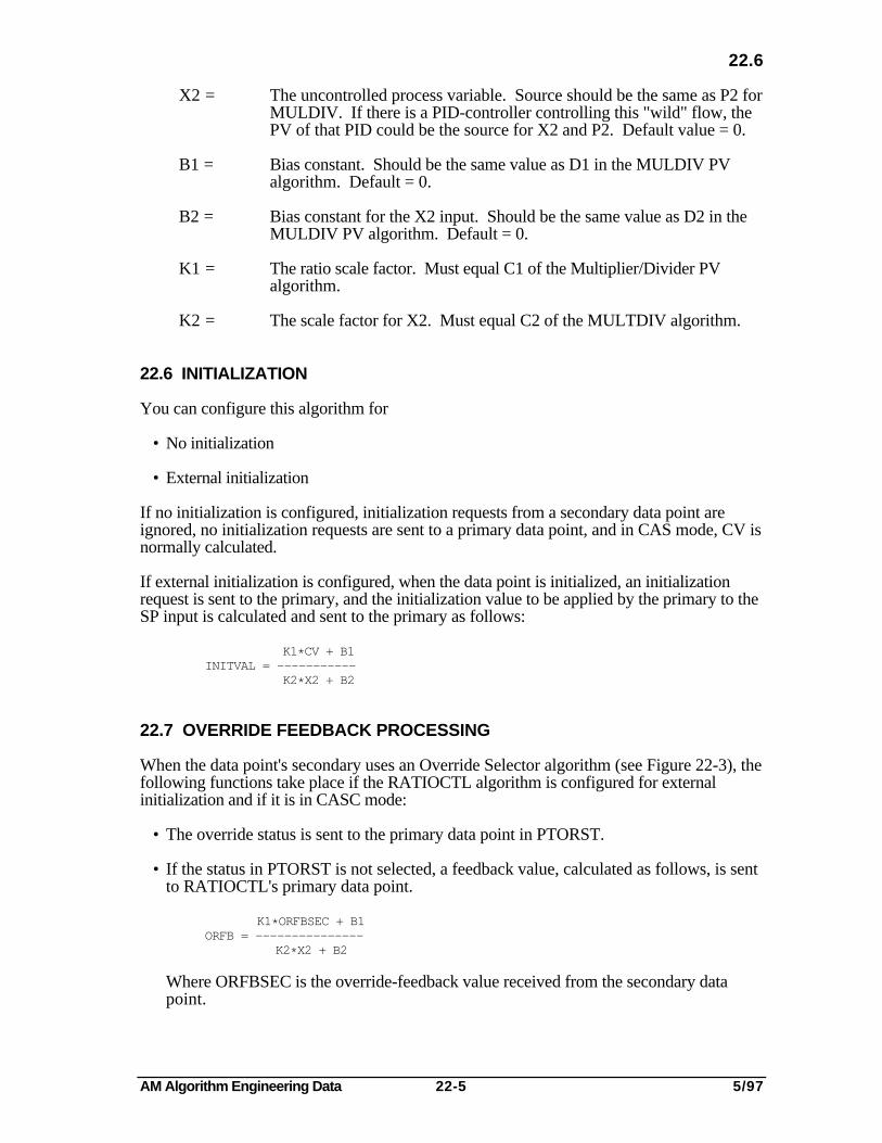
AM Algorithm Engineering Data 22-5 5/97
22.6
X2 = The uncontrolled process variable. Source should be the same as P2 forMULDIV. If there is a PID-controller controlling this "wild" flow, thePV of that PID could be the source for X2 and P2. Default value = 0.
B1 = Bias constant. Should be the same value as D1 in the MULDIV PValgorithm. Default = 0.
B2 = Bias constant for the X2 input. Should be the same value as D2 in theMULDIV PV algorithm. Default = 0.
K1 = The ratio scale factor. Must equal C1 of the Multiplier/Divider PValgorithm.
K2 = The scale factor for X2. Must equal C2 of the MULTDIV algorithm.
22.6 INITIALIZATION
You can configure this algorithm for
• No initialization
• External initialization
If no initialization is configured, initialization requests from a secondary data point areignored, no initialization requests are sent to a primary data point, and in CAS mode, CV isnormally calculated.
If external initialization is configured, when the data point is initialized, an initializationrequest is sent to the primary, and the initialization value to be applied by the primary to theSP input is calculated and sent to the primary as follows:
K1*CV + B1INITVAL = ———————————
K2*X2 + B2
22.7 OVERRIDE FEEDBACK PROCESSING
When the data point's secondary uses an Override Selector algorithm (see Figure 22-3), thefollowing functions take place if the RATIOCTL algorithm is configured for externalinitialization and if it is in CASC mode:
• The override status is sent to the primary data point in PTORST.
• If the status in PTORST is not selected, a feedback value, calculated as follows, is sentto RATIOCTL's primary data point.
K1*ORFBSEC + B1ORFB = ———————————————
K2*X2 + B2
Where ORFBSEC is the override-feedback value received from the secondary datapoint.
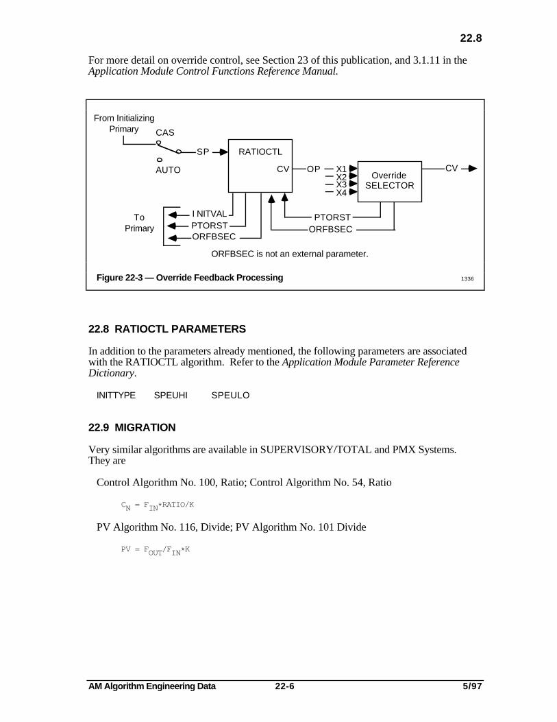
AM Algorithm Engineering Data 22-6 5/97
22.8
For more detail on override control, see Section 23 of this publication, and 3.1.11 in theApplication Module Control Functions Reference Manual.
From InitializingPrimary CAS
AUTO
SP RATIOCTL
CV OP X1X2X3X4
OverrideSELECTOR
I NITVALPTORSTORFBSEC
ToPrimary
CV
PTORSTORFBSEC
ORFBSEC is not an external parameter.
Figure 22-3 — Override Feedback Processing 1336
22.8 RATIOCTL PARAMETERS
In addition to the parameters already mentioned, the following parameters are associatedwith the RATIOCTL algorithm. Refer to the Application Module Parameter ReferenceDictionary.
INITTYPE SPEUHI SPEULO
22.9 MIGRATION
Very similar algorithms are available in SUPERVISORY/TOTAL and PMX Systems.They are
Control Algorithm No. 100, Ratio; Control Algorithm No. 54, Ratio
CN = FIN*RATIO/K
PV Algorithm No. 116, Divide; PV Algorithm No. 101 Divide
PV = FOUT/FIN*K
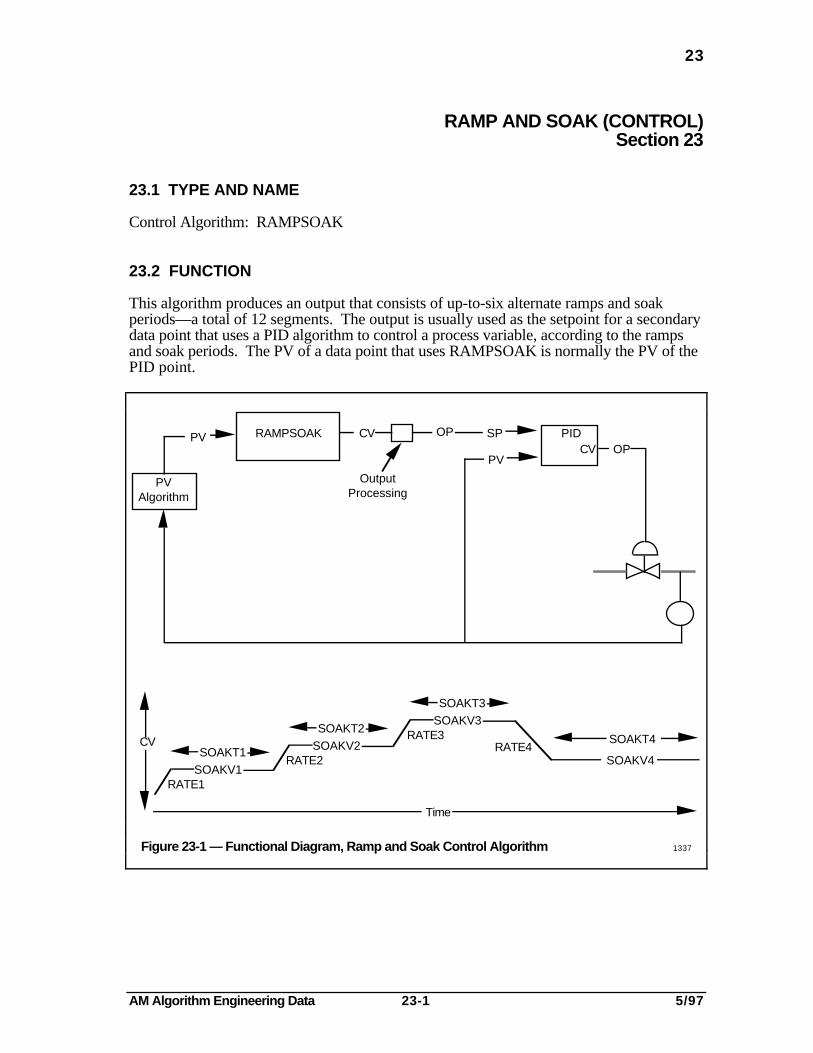
AM Algorithm Engineering Data 23-1 5/97
23
RAMP AND SOAK (CONTROL)Section 23
23.1 TYPE AND NAME
Control Algorithm: RAMPSOAK
23.2 FUNCTION
This algorithm produces an output that consists of up-to-six alternate ramps and soakperiods—a total of 12 segments. The output is usually used as the setpoint for a secondarydata point that uses a PID algorithm to control a process variable, according to the rampsand soak periods. The PV of a data point that uses RAMPSOAK is normally the PV of thePID point.
PV RAMPSOAK
PVAlgorithm
CV OP SP
PV
OutputProcessing
PIDCV OP
SOAKV1RATE1
SOAKT1 SOAKV2RATE2
SOAKT2SOAKV3
RATE3
SOAKT3
SOAKV4
SOAKT4RATE4
Time
CV
Figure 23-1 — Functional Diagram, Ramp and Soak Control Algorithm 1337
AM Algorithm Engineering Data 23-2 5/97
23.3
Once started the whole sequence of six ramps and six soak periods repeats itself, if it is notstopped by an operator or by a user-written program. A Universal Station operator can putthe point in MANual mode to freeze the sequence, and then return it to AUTO to continuethe sequence.
23.3 USE
RAMPSOAK is principally used for automatic temperature cycling in furnaces and ovens.It can also be used for automatic startup of units, and for simple batch-sequence controlwhere the batch sequence is part of a process that is otherwise a continuous process.
23.4 OPTIONS AND SPECIAL FEATURES
23.4.1 Operational Features
The operating modes establish the operating state of the RAMPSOAK algorithm as follows:
• MAN—The sequence is stopped and the timers are not running.
• AUTO—The sequence is running.
• CAS—The sequence and timers are reset.
Further functions in each mode are the following:
• MAN mode
– The timers are stopped and hold the last value.
– The value in CV is replaced by the OP value (after converting to EUs).
– SP = CV (SP doesn't affect the output but can be seen at Universal Stations anduser-written programs).
• AUTO Mode
– If the current segment is a ramp, and if the guaranteed ramp conditions are OK (see23.4.4),
CV changes at the ramp rate.
If CV should overshoot the next soak value, it is clamped at that value, and theremaining soak-time (REMSOAKT), the current-segment (CURSEGID), andthe mark timers and flags (see 23.4.5) are updated.
– If the guaranteed ramp conditions are not OK, the mark timers (see 23.4.5) arestopped.
AM Algorithm Engineering Data 23-3 5/97
23.4.2
– If the current segment is a soak, and if the point just changed from MAN toAUTO, or just started the soak segment, and the guaranteed soak time conditionsare not OK (see 23.4.3),
The soak timer doesn't start.
CV remains at its last value.
The mark timers (see 23.4.5) are stopped.
– If the guaranteed soak-time conditions are OK,
The soak timer begins to run or continues to run.
CV holds at its last value and the mark timers and flags (see 23.4.5) areupdated.
The remaining soak time (REMSOAKT) is adjusted.
If the soak timer times out, the current segment (CURSEGID) becomes the nextramp segment.
– In any case, in AUTO mode SP is equal to CV. SP doesn't affect the output butcan be seen at Universal Stations and by user-written programs.
• CAS Mode
– CV is equal to SP, the current segment (CURSEGID) is Ramp1, the remainingsoak time (REMSOAKT) is zero, and all timers are reset.
23.4.2 Changing Remaining Soak Time and Current Segment
When the RAMPSOAK point is in MAN mode, an operator at a Universal Station canchange the remaining soak time (REMSOAKT) if the current segment is a soak.
Also, when the point is in MAN mode, an operator can change the current segment(CURSEGID).
When the mode is returned to AUTO the sequence continues, as modified by thesechanges. If the segment was changed, the sequence resumes with the new segment, whichcan be a ramp or a soak.
Because changes to these parameters don't change the mark functions (see 23.4.5), exceptif CURSEGID is a lower segment than the mark segment (SnSEGID), operators shouldnot be allowed to change REMSOAKT or CURSEGID when the mark functions areconfigured.
23.4.3 Guaranteed Soak Time
This feature guarantees that the PV is at the proper soak value before the soak-timemeasurement begins.

AM Algorithm Engineering Data 23-4 5/97
23.4.4
If, when a soak segment begins or is resumed by switching from MAN to AUTO, the PVis not within a user-specified deviation (MXSOKDEV) from the SP value (SP alwaysequals CV), the soak timer doesn't start. When the deviation is within the MXSOKDEVvalue, the timer is started and continues, even if the deviation again exceeds MXSOKDEV.
Because the PV could be above or below SP, it is the absolute value of the deviation that ischecked against MXSOKDEV.
To bypass this check you can change MXSOKDEV to NaN. This check is also bypassedif you don't configure a PV algorithm (select the NULL PV algorithm).
The soak timer can also be kept from starting when HOLDCMD contains On. This allowsyou to use a general-input connection to HOLDCMD or a write to HOLDCMD by a CLblock, to hold the soak timer until some other condition is met. Again, once the timer startsit continues, regardless of the deviation or the value in hold.
HOLDCMD also affects the guaranteed ramp function. See 23.4.4.
23.4.4 Guaranteed Ramp Rate
This feature guarantees that the PV keeps up with the desired value indicated by SP (SPalways tracks CV).
You can specify a maximum ramp-deviation value in MXRMPDEV. There are twoconditions that cause the ramp to stop to wait for the PV to catch up with SP. They are
• RATEn > 0
and
PV < (SP - MXRMPDEV)
• RATEn < 0
and
PV > (SP + MXRMPDEV)
These checks are bypassed if MXRMPDEV contains NaN or if this data point doesn't use aPV algorithm (the NULL PV algorithm is configured).
Another condition that stops the ramp is HOLDCMD containing On. You can use ageneral-input connection to HOLDCMD or a write to HOLDCMD by a CL block to stop orhold the ramp until some condition that you specify is met.
The content of HOLDCMD also affects the guaranteed soak-time feature. See 23.4.3.

AM Algorithm Engineering Data 23-5 5/97
23.4.5
23.4.5 Mark Timer Functions
Two flags are provided with the RAMPSOAK algorithm to indicate to other data points orto a CL block that a specified time has elapsed from the beginning of a specified rampsegment or soak segment. These mark-timer flags are S1 and S2.
Each of these flags is associated with three parameters that specify the segment, the timeafter the beginning of the segment, and the time from the beginning of the segment until theend time. These parameters are as follows:
Flag Segment Beginning Time End Time
S1 S1SEGID S1BGNTIM S1ENDTIM
S2 S2SEGID S2BGNTIM S2ENDTIM
The S1 or S2 flag is turned on at the number of minutes after the specified segment begins,as is specified in SnBGNTIM. The corresponding flag is turned Off at the number ofminutes after the specified segment begins, as specified in SnENDTIM.
The following functions also take place:
• At the end of the last segment in the sequence, the S1 and S2 flags are turned Off andthe timers are reset.
• When a ramp or a soak segment is held up by the guaranteed-ramp or the guaranteed-soak functions, the mark timers are stopped.
• The mark timers stop when the data point is in MAN mode and the S1 and S2 flags areunchanged.
• If the remaining soak time (REMSOAKT) is changed (in MAN mode), the mark timersare not affected.
• If the current segment (CURSEGID) is changed (in MAN mode) to a segment that isearlier than a segment specified by SnSEGID, the corresponding mark flag goes to Offand its timers are reset. If a later segment is specified in CURSEGID, the flags andtimers are not affected.
23.4.6 Achieving Longer Sequences by Interconnecting RAMPSOAK Points
A sequence of more than 12 ramp and soak segments can be attained by interconnectingRAMPSOAK points as shown on Figure 23-2.
OP from point A is sent to point B by a control-output connection from point A. The CVof point B is sent to SP of point A by a control-input connection in point A. The output(OP) of point B is sent to its secondary (usually a PID point) through a control-outputconnection. Control-output connections from point B to other secondaries can be made,but none should go to point A—point A gets point B's CV by a control-input connection.

AM Algorithm Engineering Data 23-6 5/97
23.4.7
RAMPSOAKPOINT A
RAMPSOAKPOINT A
SP OP SP
AUTO/CAS CAS/AUTO
CVOP To Secondary
(Normally a PIDPoint)
Figure 23-2 — Interconnecting RAMPSOAK Points for Longer Sequences 1338
Point B should be configured for external initialization and point A should be configuredfor internal initialization.
Only one of the RAMPSOAK points should be in AUTO mode at any time. The othershould be in CAS mode. The point in AUTO mode goes through its sequence, and at theend of the last segment, it is switched to CAS mode and its timers are reset. At the sametime, the other point is switched to AUTO and proceeds through its sequence.
The automatic mode switching can be achieved by configuring a mark flag (see 23.4.5) ineach point, to go on just before the end of its sequence. The RAMPSOAK points exchangemark flags through general-input connections and the flags change the modes throughexternal mode-switching. See Section 4 in the System Control Functions manual.
23.4.7 How to Get Just One Sequence
In normal operation, the sequence of ramp and soak segments repeats itself as long as theRAMPSOAK point is left in AUTO mode. An operator at a Universal Station can suspenda sequence by changing the mode to MAN, or he or she can reset the sequence by changingthe mode to CAS.
A mark flag (see 23.4.5) can be used to switch the mode to MAN or to CAS at any time ina sequence, including at the end of a single sequence. The flag is used to change the modethrough external mode-switching. See Section 4 in the System Control Functions manual.
23.4.8 Changes of SP by Operators or User-Written Programs
Universal Station operators and user-written programs can change the SP value with noerror indication, but the next time the RAMPSOAK point is processed, SP again equalsCV. SP tracks CV so that SP can be used for the guaranteed ramp and guaranteed soakfunctions. See 23.4.3 and 23.4.4.

AM Algorithm Engineering Data 23-7 5/97
23.4.9
23.4.9 Notes on Ranges and Limits
In MAN and AUTO modes, SP limits are ignored. To avoid confusion, and to haveconsistent operation in CAS mode, the SP limits should be configured as NaN.
If the RAMPSOAK data point uses a PV algorithm, the setpoint EU range is the same asthe PV EU range, and can't be differently configured. You should configure this point'sPV EU range to be the same as the SP EU range of the secondary point that is receivingthis point's output. If the RAMPSOAK point doesn't use a PV algorithm, you shouldconfigure its SP EU range to be the same as that of the SP of the secondary point.
The deviation limits (MXRMPDEV and MXSOKDEV) apply to all segments in thesequence. If you need different deviation limits in different segments, you can configureMXRMPDEV and MXSOKDEV as NaN and use a CL block and the HOLD flag (see23.4.3 and 23.4.4) to take over the functions of these deviation limits.
23.4.10 Restart or Point Activation
On a cold restart, a warm restart, or when the data point is activated, the mode goes toMAN and the CV value is NaN. All timers are reset, and the current segment ID is madeequal to the first ramp segment.
No special action occurs on a hot restart and the operation continues from where it was.
23.5 Equations
There are no configurable equations for the RAMPSOAK algorithm. The ramp and soaksegments are specified in the following parameters (also see Figure 23-1):
• Number of ramp/soak segment-pairs in the sequence—NORSSEQDefault = 2.
• Ramp Rates, EUs per minute—RATE1 through RATE6Default = NaN
• Soak values—SOAKV1 through SOAKV6Default = NaN
• Soak times, in minutes—SOAKT1 through SOAKT6Default = 0
23.6 INITIALIZATION
You can configure this algorithm for
• Internal Initialization
• External Initialization

AM Algorithm Engineering Data 23-8 5/97
23.7
If internal initialization is configured, when an initializing condition occurs, no initializationrequest is sent to a primary data point and the RAMPSOAK point holds in the present stateand resumes normal processing when initialization is finished.
If external initialization is configured, an initializing condition has the same effect on theRAMPSOAK point, except that it sends an initialization request to any primary pointconnected to this point's SP. See 23.4.6.
23.7 OVERRIDE FEEDBACK PROCESSING
This algorithm does not participate in override-feedback processing.
23.8 RAMPSOAK PARAMETERS
All of the significant parameters associated with the RAMPSOAK algorithm have beendescribed. Refer to the Application Module Parameter Reference Dictionary for additionalparameter information.
23.9 MIGRATION
There are similar ramp and soak algorithms in SUPERVISORY/TOTAL and PMX Systemsand in Extended Controllers. They compare as shown in Table 23-1.
Table 23-1 — Comparison of SUPERVISORY/TOTAL and PMX Algorithms with RAMPSOAK
ITEM EXT. CONTROLLER S/T-PMX AM
Algorithm No. 34 Control No. 70 RAMPSOAK
Max. No. Segments 6 8 6(ramps plus soaks)
Modes MAN Stop Stop StopCAS Ready N/A ResetAUTO Sequence CN = OP SequenceCOMP N/A Sequence N/A
Start Value Init. or bump Starts @ SP Init. or bump
Guar. Ramp & Yes Yes YesGuar. Soak?
Override Strategy? Yes No No
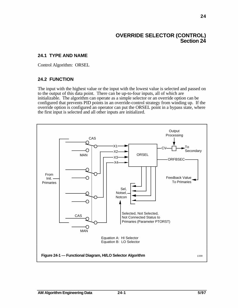
AM Algorithm Engineering Data 24-1 5/97
24
OVERRIDE SELECTOR (CONTROL)Section 24
24.1 TYPE AND NAME
Control Algorithm: ORSEL
24.2 FUNCTION
The input with the highest value or the input with the lowest value is selected and passed onto the output of this data point. There can be up-to-four inputs, all of which areinitializable. The algorithm can operate as a simple selector or an override option can beconfigured that prevents PID points in an override-control strategy from winding up. If theoverride option is configured an operator can put the ORSEL point in a bypass state, wherethe first input is selected and all other inputs are initialized.
CV
ORFBSECORSEL
OutputProcessing
ToSecondary
Feedback ValueTo Primaries
Selected, Not Selected,Not Connected Status toPrimaries (Parameter PTORST)
X1
X2
X3X4
CAS
MAN
CAS
MAN
Sel,Notsel,Notcon
FromInit.
Primaries
Equation A: HI SelectorEquation B: LO Selector
Figure 24-1 — Functional Diagram, HI/LO Selector Algorithm 1339
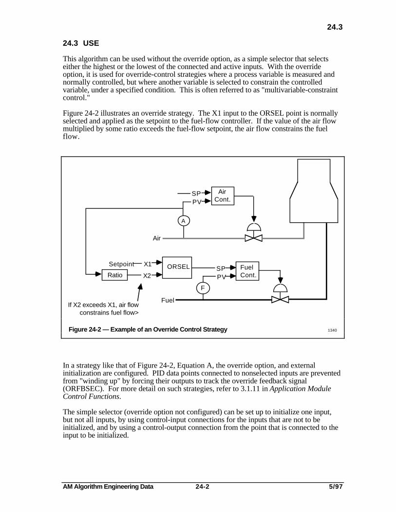
AM Algorithm Engineering Data 24-2 5/97
24.3
24.3 USE
This algorithm can be used without the override option, as a simple selector that selectseither the highest or the lowest of the connected and active inputs. With the overrideoption, it is used for override-control strategies where a process variable is measured andnormally controlled, but where another variable is selected to constrain the controlledvariable, under a specified condition. This is often referred to as "multivariable-constraintcontrol."
Figure 24-2 illustrates an override strategy. The X1 input to the ORSEL point is normallyselected and applied as the setpoint to the fuel-flow controller. If the value of the air flowmultiplied by some ratio exceeds the fuel-flow setpoint, the air flow constrains the fuelflow.
Air
A
SPPV
AirCont.
FuelCont.
SPPV
F
Fuel
Ratio
Setpoint ORSELX1
X2
If X2 exceeds X1, air flowconstrains fuel flow>
Figure 24-2 — Example of an Override Control Strategy 1340
In a strategy like that of Figure 24-2, Equation A, the override option, and externalinitialization are configured. PID data points connected to nonselected inputs are preventedfrom "winding up" by forcing their outputs to track the override feedback signal(ORFBSEC). For more detail on such strategies, refer to 3.1.11 in Application ModuleControl Functions.
The simple selector (override option not configured) can be set up to initialize one input,but not all inputs, by using control-input connections for the inputs that are not to beinitialized, and by using a control-output connection from the point that is connected to theinput to be initialized.

AM Algorithm Engineering Data 24-3 5/97
24.4
NOTE
There are some important guidelines that must be observed when configuring an override-control strategy. See 3.1.11 in Application Module Control Functions.
24.4 OPTIONS AND SPECIAL FEATURES
24.4.1 Override and Bypass Options
If the override option is configured, external initialization must also be configured. In thisconfiguration, PID points connected to nonselected inputs are prevented from "winding up"by forcing their outputs to track the override-feedback signal (ORFBSEC).
If the override option is configured, an operator at a Universal Station can force the X1input to be selected by storing On in the BYPASS parameter. When BYPASS is On, X2,X3, and X4 are initialized to the value in X1. Also, when BYPASS is On, only the X1input has to have a Normal-value status in order for normal override-feedback processingto take place.
An operator can turn BYPASS on and off at any time. When BYPASS is changed fromOff to On, X2, X3, and X4 go into initialization. When it is changed from On to Off, X2,X3, and X4 come out of initialization.
24.4.2 Restrictions
The engineering-units range for the X1 through X4 inputs must be configured inparameters XEUHI and XEULO. These parameters contain the high and low values forthe range, which is the same for all four inputs.
External initialization must be configured if the override option is configured.
24.4.3 Operating Modes
Because a data point that uses ORSEL is always a secondary to at least one other datapoint, this algorithm operates only in the following modes:
• CAS
• MAN
24.4.4 Restart or Point Activation
On a cold or a warm restart, or on activating the data point, ORSEL operates normallyunless it is configured for external initialization. If it is, CV is initialized to the valuereturned from the secondary and an initialization request is sent to all of the primaries.
On a hot restart, ORSEL resumes normal operation.

AM Algorithm Engineering Data 24-4 5/97
24.4.5
24.4.5 Error Handling
In CAScade mode with BYPASS Off, if any input has a Bad-value status, CV's value isbad (NaN) (the mode doesn't change when the CV value goes bad). If BYPASS is On,only the X1 input needs to be Normal in order for CV to be calculated normally.
If a Bad input, which was causing CV to be Bad, returns to Normal, CV returns to normaland one of the following occurs:
• If no initialization is configured, CV is normally determined and the primaries are notinitialized.
• If external initialization is configured, CV is made equal to OP and the primaries areinitialized.
24.5 EQUATIONS
There are two equation choices:
• Equation A—Select the higher of the connected, active inputs.
CV = highest of X1 through Xm
• Equation B—Select the lower of the connected, active inputs.
CV = lowest of X1 through Xm
Where
CV = The control-algorithm output in engineering units
X1 through X4 = The four available inputs
m = The number of inputs configured
For either equation
SELXINP = The selected input: SELECTX1 through SELECTX4. If more thanone input has the highest (EqA) or the lowest (EqB) value, the lower-numbered input is selected, e.g., if X2 and X3 have exactly the samehighest value (EqA) SELXINP contains SELECTX2.
24.6 INITIALIZATION
You can configure this algorithm for
• No initialization
• External initialization
If no initialization is configured, CV and SELXINP are normally calculated, andinitialization requests from secondary points are ignored.
AM Algorithm Engineering Data 24-5 5/97
24.7
If external initialization is configured, the mode is CAS, the output is disposable, theoverride option is configured, and BYPASS is true; an initialization request from thesecondary is passed on to the primaries connected to X2, X3, and X4 with an initializationvalue equal to CV.
SELECTX1 is placed in SELXINP.
If external initialization is configured and ORSEL is initialized because it is in MANualmode, the output is indisposable, or it has just returned from bad control status; CV ismade equal to INITVAL from the secondary, an initialization request is passed on to allprimaries with an initialization value equal to CV, and SELXINP contains None.
24.7 OVERRIDE FEEDBACK PROCESSING
24.7.1 Override Feedback Initiation
See Figure 24-1. If the override option is configured for the ORSEL point, externalinitialization must also be configured. Where both conditions are true, and when theORSEL point is in CAScade mode and not initializing, it propagates override feedbackinformation to its primary points and on "upstream."
When BYPASS is Off, the appropriate NotCon, Sel, NotSel status is given to ORSEL'sprimaries in PTORST, and the override feedback value that is passed to the primaries iscalculated as follows:
ORFBSEC = CV
If, under the above conditions, BYPASS is On, the status sent to the primary connected toX1 is SEL, NOTCON is sent to all other primaries and they are all initialized.
If there is more than one Override Feedback data point in a strategy, only the one nearestthe final control element (the "most downstream" point) initiates override feedback.
24.7.2 Override Feedback Propagation
Override feedback propagation is the passing of status and feedback values, from theinitiating Override Feedback Selector, "upstream" through one or more other data points.
If a "downstream" Override Feedback Selector requests status and value propagation, an"upstream" Override Feedback Selector" propagates the value and status "upstream," onlyif
• it is configured as an Override Selector (override option and external initializationconfigured), and
• it is in CAS mode, and
• its output is disposable.
If so,ORFB = ORFBSEC
Where ORFBSEC is the feedback value from the secondary.
And, PTORST status sent to the selected primary is the same as that received from thesecondary. If BYPASS is false, the status to all other primaries is NOTSEL. If BYPASSis true, nonselected inputs are initialized, so the status sent to them is NOTCON.
AM Algorithm Engineering Data 24-6 5/97
24.8
24.8 ORSEL PARAMETERS
In addition to the parameters already mentioned, the following parameters are associatedwith the ORSEL algorithm. Refer to the Application Module Parameter ReferenceDictionary.
CTLEQN INITTYPE OROPT XnSTS
24.9 MIGRATION
There are similar algorithms in PMX and SUPERVISORY/TOTAL systems; they are theOverride Selectors in Basic Controllers, Multifunction Controllers, and ExtendedControllers. The Override Selector algorithms in the controllers, and important differencesfrom the AM HI/LO Selector algorithm are as follows:
• Basic Controller and Multifunction Controller
Algorithm No. 21, Override High Selector—Selects the highest of up-to-eight inputs.Operates in MAN, AUTO, and CAS modes. Operation is the same in AUTO andCAS.
Algorithm No. 22, Override Low Selector—Same as No. 21 but selects the lowest ofup-to-eight inputs.
• Extended Controller
Algorithm No. 21, Selector/Override/DDC—Equation A selects the highest of up-to-six inputs and Equation B selects the lowest of up-to-six inputs. Initialization valuesare propagated to unselected input data points (slots) every other processing time.Operates in MAN, AUTO, and CAS modes. Also can accept output from the DataHiway when COMP function is enabled (DDC output). (In systems with an LCN,operating modes are MAN, AUTO, CAS, and BCAS. In CAS mode, OP is suppliedby a module on the LCN, such as an AM. BCAS is the back-up-cascade mode thatthe algorithm can operate in if OP from the LCN is not available.)

AM Algorithm Engineering Data 25-1 5/97
25
SUMMER (CONTROL)Section 25
25.1 TYPE AND NAME
Control Algorithm: SUMMER
25.2 FUNCTION
This algorithm calculates an output value that is the scaled sum of up to three inputvariables. A bias value can be included in the sum.
Two equations are available. One adds a single scaled input to the bias value. The otheradds up to four scaled inputs, multiplies the result by an overall scale factor, and adds thebias value.
This algorithm is similar to PV-algorithm SUMMER (Section 10).
SUMMER
CAS
AUTO
SP
From InitializingPrimary
Operator orUser-Written
Program
ToPrimary
ToSecondary
OutputProcessing
CV OP
INITVAL
X2X3X4
Equations: A; CV = K SP + BB; CV = K (K1 SP + K2 X2 + ... + Km Xm) + B
*** * *
Figure 25-1 — Functional Diagram, Summer Control Algorithm 1341
25.3 USE
This algorithm is normally part of a cascade-control strategy. It can be used to calculate asum of up to four control inputs. It can provide an input to an override-selector algorithm.

AM Algorithm Engineering Data 25-2 5/97
25.4
25.4 OPTIONS AND SPECIAL FEATURES
25.4.1 Single Input Sum and Four Input Sum
Equation A multiplies a single input by a scale factor and adds the result to the bias value.Equation B multiplies up to four inputs by individual scale factors, adds these products,multiplies the result by an overall scale factor and adds the bias value to the result.
In both equations, the SP input is initializable.
25.4.2 Operating Modes
This algorithm operates in the following modes:
• MAN
• AUTO
• CAS
25.4.3 Restart or Point Activation
For a cold or a warm restart or when this data point is reactivated, initialization takes placeas described under 25.6. For a hot restart, normal operation resumes.
25.4.4 Error Handling
If any of the SP and X1 through Xm inputs has a bad-value status, the CV-value statusgoes bad, and the point continues in the present mode. When the bad input returns tonormal, the CV status goes to normal, and if so configured, external initialization takesplace (see 25.6).
25.4.5 Setpoint Value Range
You must configure SPEULO and SPEUHI to specify the SP value range.
25.5 EQUATIONS
You can choose one of two equations:
Equation A
CV = K*SP + B
Equation B
CV = K*(K1*SP + . . . + Km*Xm) + B
AM Algorithm Engineering Data 25-3 5/97
25.6
Where
CV = The control output in engineering units
B = Bias value. Default = 0.
K = Overall scale factor. Default = 1.0.
K1 through Km = Scale factors for SP through the actual number of inputs used.Default for each = 1.0.
M = No of inputs. Default = 2.
SP = The setpoint in engineering units. This input is initializable.
X2 through Xm = Control inputs X2 through the actual number of inputs used.These are usually obtained through control-input connections.
25.6 INITIALIZATION
You can configure this algorithm for
• No initialization
• Internal initialization
• External initialization
25.6.1 Initialization Equations
When configured for no initialization, CV is normally calculated, initialization requestsfrom secondaries are ignored, and initialization requests are not sent to primaries.
When configured for internal initialization, the bias (B) is "back-calculated":
Equation A B = CV - K*SP
Equation B B = CV - K(K1*SP + . . . + Km*Xm)
When configured for external initialization, the value of SP needed to maintain CV at thepresent value is calculated and passed as INITVAL to the primary with an initializationrequest:
Equation A INITVAL = (CV - B)/K
1 (CV - B)Equation B INITVAL = ————*[———————— - (K2*X2 + . . . + Km*Xm)]
K1 K

AM Algorithm Engineering Data 25-4 5/97
25.7
25.7 OVERRIDE FEEDBACK PROCESSING
If this data point's secondary is an Override Selector point and if this point is configuredfor initialization and is in CAS mode, when override-feedback processing takes place,override status and an override value are passed to this point's primary. The status is inparameter PTORST. The feedback value is calculated as follows:
Equation A
ORFBSEC - BORFB = ———————————
K
Equation B
1 ORFBSEC - BORFB = ——*[———————————— - K2*X2 - . . . - Km*Xm]
K1 K
25.8 SUMMER PARAMETERS
In addition to the parameters already mentioned, the following parameters are associatedwith the SUMMER algorithm. Refer to the Application Module Parameter ReferenceDictionary:
INITTYPE SPSTS XnSTS
25.9 MIGRATION
Three control algorithms in SUPERVISORY/TOTAL Systems have similar functions.Two of the three are also available in PMX Systems. Table 25-1 compares them.
Table 25-1 — Comparison of SUPERVISORY/TOTAL and PMX Algorithms
NearestAM
Equation
S-T/PMXAlgorithmNumber
S-T/PMXEquation inAM Terms
S-T/PMXEquation as shownin S/T-PMX Pubs.
B 30† CV = K1*X1 + K2*X2 + B CN = K1*X + KA*Y + K2
B 50 CV = X1 + X2 + B CN = PV + P + KA
B 51 CV = X1 + X2 + B CN = PV + P + KA
†Not available in PMX systems. This algorithm can be implemented in a Basic Controller or in theSUPERVISORY/TOTAL computer.
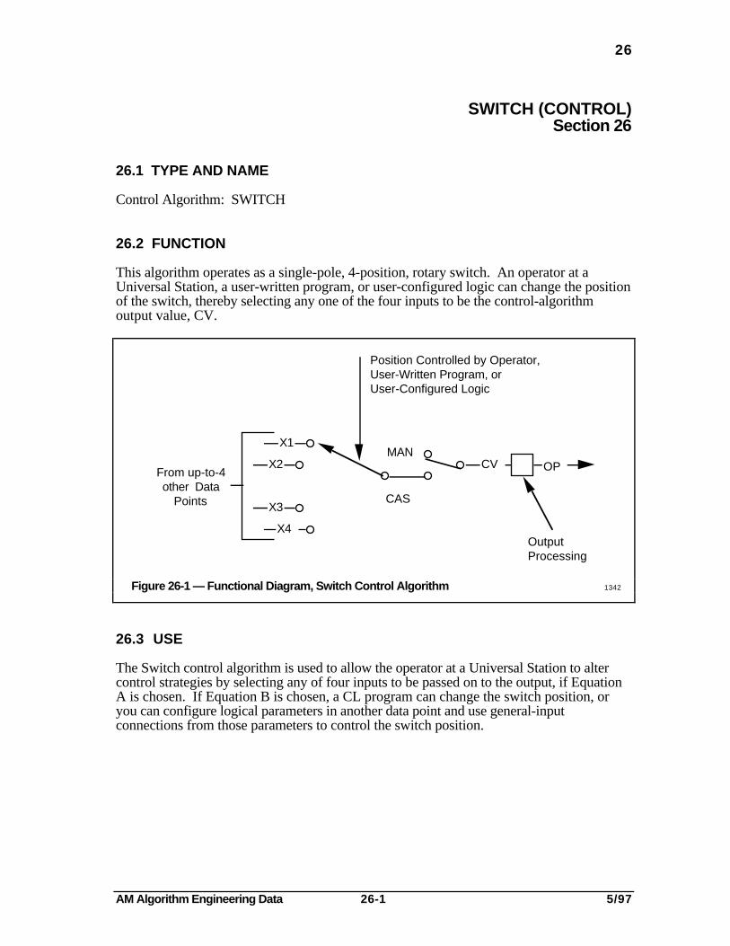
AM Algorithm Engineering Data 26-1 5/97
26
SWITCH (CONTROL)Section 26
26.1 TYPE AND NAME
Control Algorithm: SWITCH
26.2 FUNCTION
This algorithm operates as a single-pole, 4-position, rotary switch. An operator at aUniversal Station, a user-written program, or user-configured logic can change the positionof the switch, thereby selecting any one of the four inputs to be the control-algorithmoutput value, CV.
Position Controlled by Operator,User-Written Program, orUser-Configured Logic
From up-to-4other Data
Points
X1
X2
X3
X4
CV OPMAN
CAS
OutputProcessing
Figure 26-1 — Functional Diagram, Switch Control Algorithm 1342
26.3 USE
The Switch control algorithm is used to allow the operator at a Universal Station to altercontrol strategies by selecting any of four inputs to be passed on to the output, if EquationA is chosen. If Equation B is chosen, a CL program can change the switch position, oryou can configure logical parameters in another data point and use general-inputconnections from those parameters to control the switch position.
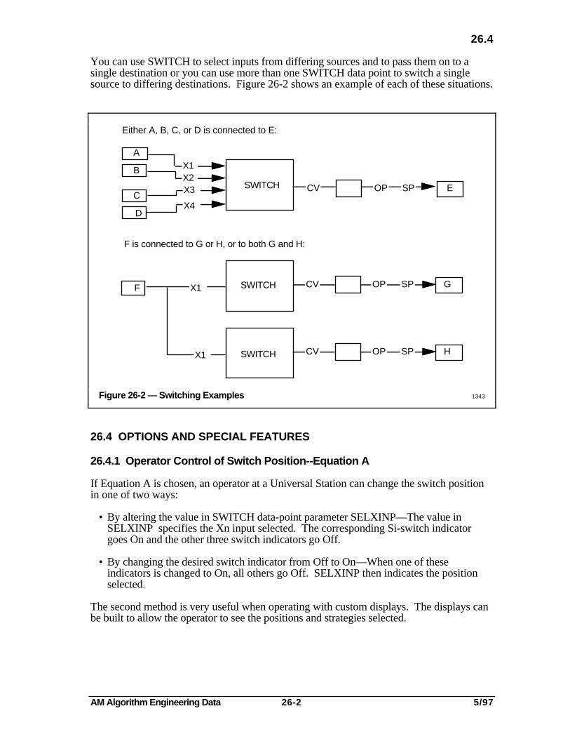
AM Algorithm Engineering Data 26-2 5/97
26.4
You can use SWITCH to select inputs from differing sources and to pass them on to asingle destination or you can use more than one SWITCH data point to switch a singlesource to differing destinations. Figure 26-2 shows an example of each of these situations.
X2X3
X4
A
B
C
D
SWITCH CV OP SP E
F SWITCH
SWITCHX1
F is connected to G or H, or to both G and H:
Either A, B, C, or D is connected to E:
CV OP SP G
CV OP SP H
X1
X1
Figure 26-2 — Switching Examples 1343
26.4 OPTIONS AND SPECIAL FEATURES
26.4.1 Operator Control of Switch Position--Equation A
If Equation A is chosen, an operator at a Universal Station can change the switch positionin one of two ways:
• By altering the value in SWITCH data-point parameter SELXINP—The value inSELXINP specifies the Xn input selected. The corresponding Si-switch indicatorgoes On and the other three switch indicators go Off.
• By changing the desired switch indicator from Off to On—When one of theseindicators is changed to On, all others go Off. SELXINP then indicates the positionselected.
The second method is very useful when operating with custom displays. The displays canbe built to allow the operator to see the positions and strategies selected.

AM Algorithm Engineering Data 26-3 5/97
26.4.2
26.4.2 Program Control of Switch Position—Equation B
If Equation B is chosen, an operator cannot change the switch position, but a CL programor general-input connections from logic parameters can. The SELXINP parameterindicates the present switch position, but it cannot be directly changed by the program orinput connections.
The switch position is changed by storing On and Off in the Si parameters as follows:
S1 S2 S3 S4 Xn SELXINP
On - - - X1 SELECTX1Off On - - X2 SELECTX2Off Off On - X3 SELECTX3Off Off Off On X4 SELECTX4
Where "-" means On or Off does not affect the switch position.
With Equation B, turning an Si indicator On does not turn the others off, as it does withEquation A.
26.4.3 Tracking Option
You can configure the SWITCH algorithm for the tracking option, which causesnonselected inputs to track the selected input value. This allows the switch position to bechanged without "bumping" the output. (Bumpless mode switching is accomplished by theExternal Initialization option. See 26.6.)
Proper operation of the tracking option requires that External Initialization be configured sothat the primaries connected to nonselected inputs can be initialized. Should one of themnot accept the initialization value from the SWITCH data point, the output may bump whenthat input is selected. (A primary might not accept an initialization value because it hasmore than one secondary and accepts external initialization from one of its othersecondaries.)
When SWITCH is included in an override control strategy, the tracking option must beconfigured.
26.4.4 Operational Modes
The Switch-control algorithm operates in the following modes:
• MANual
• CAScade
26.4.5 Restart or Point Activation
On a cold or warm restart, or when the SWITCH data point is activated, initialization takesplace, as configured. See 26.6.
On a hot restart, normal operation resumes with no initialization.
AM Algorithm Engineering Data 26-4 5/97
26.4.6
26.4.6 Error Handling
If a selected input has a bad-value status, the CV value goes bad (NaN), but the operatingmode does not change. When the status of the selected input is again good, CV isrecalculated, and if configured for external initialization, an initialization request is sent tothe primary data point.
26.4.7 Input Value Range
You must configure the X-input range in XEULO and XEUHI.
26.5 EQUATIONS
Equations A and B:
CV = Xn
n = 1, 2, 3, or 4
SELXINP = the selected input, which can range from SELECTX1 throughSELECTX4.
S1 through S4 indicate the switch selection, as described under 26.4.1 or 26.4.2.
Where:
CV = The control output value in engineering units.
SELXINP = The selected-input. Default = SELECTX1.
S1 through S4 = Switch indicators
M = The number of inputs configured. Default = 2.
26.6 INITIALIZATION
You can configure the SWITCH algorithm for
• No Initialization
• External Initialization
If you select no initialization, initialization requests from a secondary data point are ignoredand initialization requests are not sent to the primaries.
If you select external initialization, when an initializing condition occurs, an initializationrequest is sent to the selected primary and the initialization value is the present CV value.
If the tracking option is configured (see 26.4.3), the nonselected primaries are continuallyinitialized.
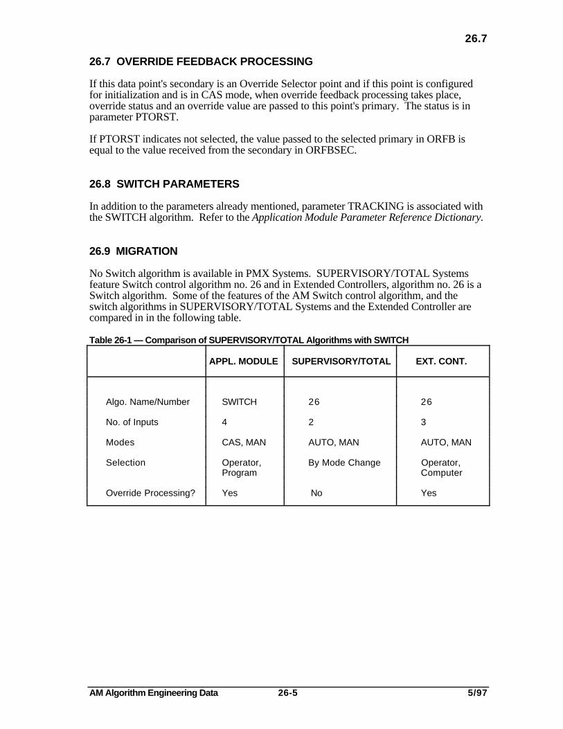
AM Algorithm Engineering Data 26-5 5/97
26.7
26.7 OVERRIDE FEEDBACK PROCESSING
If this data point's secondary is an Override Selector point and if this point is configuredfor initialization and is in CAS mode, when override feedback processing takes place,override status and an override value are passed to this point's primary. The status is inparameter PTORST.
If PTORST indicates not selected, the value passed to the selected primary in ORFB isequal to the value received from the secondary in ORFBSEC.
26.8 SWITCH PARAMETERS
In addition to the parameters already mentioned, parameter TRACKING is associated withthe SWITCH algorithm. Refer to the Application Module Parameter Reference Dictionary.
26.9 MIGRATION
No Switch algorithm is available in PMX Systems. SUPERVISORY/TOTAL Systemsfeature Switch control algorithm no. 26 and in Extended Controllers, algorithm no. 26 is aSwitch algorithm. Some of the features of the AM Switch control algorithm, and theswitch algorithms in SUPERVISORY/TOTAL Systems and the Extended Controller arecompared in in the following table.
Table 26-1 — Comparison of SUPERVISORY/TOTAL Algorithms with SWITCH
APPL. MODULE SUPERVISORY/TOTAL EXT. CONT.
Algo. Name/Number SWITCH 26 26
No. of Inputs 4 2 3
Modes CAS, MAN AUTO, MAN AUTO, MAN
Selection Operator, By Mode Change Operator,Program Computer
Override Processing? Yes No Yes

AM Algorithm Engineering Data 26-6 5/97

AM Algorithm Engineering Data 27-1 5/97
27
CL CONTROL ALGORITHM (CONTROL)Section 27
27.1 TYPE AND NAME
Control Algorithm: CL
27.2 FUNCTION
This algorithm is a user-written CL block that is like any other CL block except that it isinserted at the control-algorithm insertion point in the processing sequence (see Fig. 2-1),and it is executed instead of a standard control algorithm.
The CL block must calculate and store a control-algorithm output value in CV. Inputs tothe CL block are usually acquired by direct references in CL, but can be acquired throughgeneral inputs to a Custom Data Segment (CDS) that is included in the data point. Controlinputs cannot be configured in the Parameter Entry Display (PED) when the CL ControlAlgorithm is specified. The value placed in CV by the CL block is processed just as CV isprocessed for any other data point that uses a control algorithm.
The CL block must also compute and store an anti-windup direction in ARWDI.Propagation of windup status to the primaries is automatic. See 3.1.10 in the ApplicationModule Control Functions manual.
If this data point is part of an override strategy, the CL block must include appropriateoverride functions. See Section 23 in this publication and 3.1.11 in the ApplicationModule Control Functions manual.
Control AlgorithmProcessing
CLBlock
CV OP
SP
Inputsfrom this
and otherdata points
OutputProcessing
Figure 27-1 — Functional Diagram, CL Control Algorithm 1344
AM Algorithm Engineering Data 27-2 5/97
27.3
27.3 USE
A CL block is used when normal point processing is appropriate but none of the standardcontrol algorithms will accomplish the desired function. The CL block can be bound to asingle data point, if only one needs its functions, or it can be written as a generic CL blockand bound to several data points.
27.4 OPTIONS AND SPECIAL FEATURES
27.4.1 Restart
Normally, the CL block doesn't need to check the type of restart because the value in thePATHIND parameter (see 27.4.2) is affected by the type of restart; however, if needed, theCL block can base some specific actions on the content of the RESTART parameter.
27.4.2 Use of Key Control Subsystem Parameters
This data point provides the following standard control parameters, which should be usedappropriately by the CL block:
• CVTYPE—Configured when the point is built to indicate the type of value in CV. Itcan be EngrUnit or Percent.
• ARWDI—Configured to define the directional relationship between the output and thesetpoint. It contains Direct (SP increase causes CV increase) or Reverse (SP increasecauses CV decrease). The value can be changed by the CL block, if it needs to bechanged, based on one or more of the inputs. Default value = Direct.
• INITTYPE—Configured to indicate the type of initialization, None, Int, or Ext. If Intis configured, the CL block should do its own internal initialization, such as adjustingbias to eliminate a bump to the process. If Ext is configured, the CL block mustcalculate the value in INITVAL that the primary is to provide to this point's SP.Configure None if no initialization is necessary.
• PATHIND—Path indicator, which contains a value derived by the control subsystemthat indicates how the CL block should function on this processing pass. The valuesare as follows:
Fwd—Perform the normal forward calculation. SP is available as a standard input.Other inputs must be obtained by the CL block either by directly referring to them (asABC100.PV) or by using general inputs to bring them into a custom data segmentincluded in this point. If the value of a required input is bad, a bad-control alarmshould be generated by storing Bad in CV (see 27.4.3), but the CL block should notabort.
Init—Initialize according to the type of initialization called for in INITTYPE. IfINITTYPE contains Ext, calculate the SP from the CV and from the other inputs. CVhas already been initialized.
AM Algorithm Engineering Data 27-3 5/97
27.4.3
OR—Participate in override-feedback propagation. Override feedback propagationoccurs only on points that are “upstream” from a point using an override controlalgorithm. Also, it only occurs when the point’s mode is CAS and when INITTYPEcontains Ext. Set the primary's PTORST to the value in your own PTORST andrequest a process special of the primary by placing OR in its PPSREQ parameter. Inaddition, if PTORST indicates NotSel, compute the feedback value for the primary,based on the value received in ORFBSEC and place that value in the ORFBSEC ofthe primary point.
Hold—Hold because the point is in MANual mode or the output is indisposable. CVshould be computed as for a forward pass to continue proper handling of the bad-control situation.
NOTE
The HOLD and OR values are reserved words in CL. To use them in a CL program, place anapostrophe just before the word. For example
IF PATHIND = 'HOLD THEN EXIT
27.4.3 Error Handling
If an input used in calculating CV has a Bad-value status, the CL block should use theappropriate CL statement to declare the CV to be bad. Output processing then initiates"bad-control" handling.
27.4.4 Processing Schedule and Execution Time
The CL block should not be used to perform long, complex operations because there maynot be enough time in normal point processing to complete such operations. Points that usea CL control algorithm should be scheduled at the longest reasonable interval, and ifpossible, should be assigned to the Slow Processor. If execution of the CL block takes toomuch time, it is aborted and an alarm is generated.
27.5 EQUATIONS
The equation(s) for a CL control algorithm, if any, is a function of the CL block.
27.6 INITIALIZATION
See 27.4.2.
27.7 OVERRIDE FEEDBACK PROCESSING
See 27.4.2.
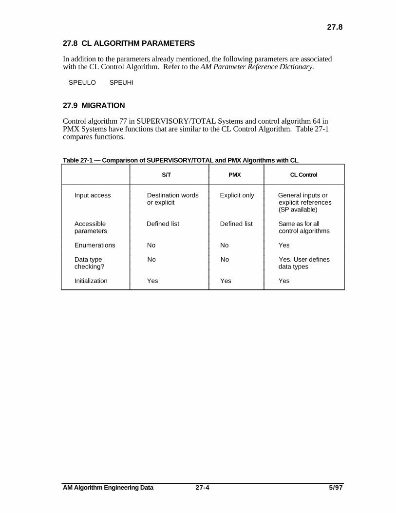
AM Algorithm Engineering Data 27-4 5/97
27.8
27.8 CL ALGORITHM PARAMETERS
In addition to the parameters already mentioned, the following parameters are associatedwith the CL Control Algorithm. Refer to the AM Parameter Reference Dictionary.
SPEULO SPEUHI
27.9 MIGRATION
Control algorithm 77 in SUPERVISORY/TOTAL Systems and control algorithm 64 inPMX Systems have functions that are similar to the CL Control Algorithm. Table 27-1compares functions.
Table 27-1 — Comparison of SUPERVISORY/TOTAL and PMX Algorithms with CL
S/T PMX CL Control
Input access Destination words Explicit only General inputs oror explicit explicit references
(SP available)
Accessible Defined list Defined list Same as for allparameters control algorithms
Enumerations No No Yes
Data type No No Yes. User defineschecking? data types
Initialization Yes Yes Yes
FAX Transmittal FAX No.: (602) 313-4842
TO: Maria Nelson Total pages:(including this page)
READER COMMENTS
Title of Document: AM Algorithm Engineering Data Issue Date: 5/97
Document Number: AM09-501
Comments:
Recommendations:
FROM:
Name: Date:
Title:
Company:
Address:
City: State: ZIP:
Telephone: FAX:
You may also call 800-822-7673 (available in the 48 contiguous states except Arizona; in Arizona dial 602-313-5558, or write to:
Honeywell Inc.Industrial Automation and ControlAutomation College2820 West Kelton LanePhoenix, AZ 85023-3028


Industrial Automation and Control Helping You Control Your World
Automation College
2820 W. Kelton Lane
Phoenix, AZ 85023-3028