Applicability of the most frequent value methodin groundwater modeling

Peter Szucs · Faruk Civan · Margit Virag

Abstract The Most Frequent Value Method (MFV) isapplied to groundwater modeling as a robust and effectivegeostatistical method. The Most Frequent Value methodis theoretically derived from the minimization of the in-formation loss called the I-divergence. The MFV algo-rithm is then coupled with global optimization (Very FastSimulated Annealing) to provide a powerful method forsolving the inverse problems in groundwater modeling.The advantages and applicability of this new approach areillustrated by means of theoretical investigations and casestudies. It is demonstrated that the MFV method hascertain advantages over the conventional statisticalmethods derived from the maximum likelihood principle.

R�sum� On a appliqu� la m�thode de la valeur la plusfr�quente (VPF) comme une m�thode g�ostatistique ro-buste et efficace pour mod�liser les eaux souterraines. Dupoint de vue th�orique, la m�thode de VPF part de laminimisation de l’information perdue, d�nomm�e I-di-vergence. On couple apr�s l’algorithme de la m�thode deVPF avec la m�thode d’optimisation globale affin der�aliser une m�thode performante pour r�soudre le pro-bl�me inverse dans le domaine des eaux souterraine. Lesavantages et les possibilit�s d’application de cette nou-velle approche sont illustr�es par des investigationsth�oriques, ainsi que par des �tudes de cas. On montre quela m�thode de VPF pr�sente certains avantages par rap-

port des m�thodes statistiques conventionnelles bas�es surle principe de la probabilit� maximale.

Resumen El M�todo del Valor Mas Frecuente (VMF), esaplicado al modelamiento de agua subterr�nea, como unm�todo geoestad�stico simple y efectivo. Este m�todo esderivado te�ricamente de la acci�n de reducir al m�nimola p�rdida de informaci�n, llamada as� divergencia – I. Elalgoritmo del VMF es entonces acoplado con optimiza-ci�n global(Very Fast Simulated Annealing), para obteneras� un m�todo efectivo que resuelva los problemas in-versos en el modelamiento de aguas subterr�neas. Lasventajas y aplicabilidad de esta aproximaci�n nueva sonilustradas a trav�s de investigaciones te�ricas y estudiosde caso. Se demuestra que el m�todo VMF tiene ciertasventajas sobre los m�todos estad�sticos convencionalesderivados del principio de la probabilidad m�xima.

Introduction

One of the main objectives of groundwater modeling is todetermine the properly working earth models in order toadequately explain the hydrogeological observations.From the mathematical point of view, such solutions canbe found by optimization (Lee 1999). Frequently, theinverse methods are used to determine the optimal pa-rameter values of the groundwater models. Adjusting theestimates of the model parameters minimizes a specialobjective function, as a measure of the misfit or error,characterizing the deviation between the measured andcalculated data. In Earth science applications, the objec-tive functions may have multiple hills and valleys in themulti-dimensional parameter space. The conventionallocal search algorithms are usually trapped in one of thelocal minima instead of approaching the global minimum(Sen and Stoffa 1995). Such limitations of the conven-tional methods for hydrogeological problems can be cir-cumvented by the application of the global optimizationmethods.

The calculated or theoretical data can be determinedfrom the solution of mathematical models by assigning aset of prescribed values to the model parameters. Thisconstitutes the forward problem. An accurate forwardproblem solution is vital for an effective inverse algo-rithm. Besides the forward and inversion problems, the

Received: 2 December 2003 / Accepted: 9 December 2004Published online: 17 February 2005

� Springer-Verlag 2005

P. Szucs ())Department of Hydrogeology and Engineering Geology,University of Miskolc,3515 Miskolc-Egyetemvaros, Hungarye-mail: hgszucs@uni-miskolc.hu

F. CivanMewbourne School of Petroleum and Geological Engineering,the University of Oklahoma,Norman, OK, 73019, USA

M. ViragVIZITERV Consult Plc.,4400 Nyiregyhaza, Josa u. 5, Hungary

Hydrogeol J (2006) 14:31–43 DOI 10.1007/s10040-004-0426-1

applied statistical principle is also a key factor in suc-cessful modeling as the objective or error functions arebased on different statistical norms and principles. Un-fortunately, the old dogma still exists in that the estima-tion or the measuring errors are approximately normally(Gaussian) distributed (Huber 1981). Therefore, the ap-plication of the least-squares principles based on themaximum likelihood theory has been widespread even ingeosciences. However, the efficiency of such classicalalgorithms is questionable when the actual error is not aGaussian distribution.

The most frequent value (MFV) procedure (Steiner1991, 1997) has been introduced as a robust and resistantmethod for geo-statistical data analysis and processing.This paper combines the MFV method with global opti-mization to provide more accuracy and reliability in pa-rameter estimation in groundwater modeling and hydro-geology problems.

Theory of inverse procedures

A synthetic data set generated from a mathematical modelusing a set of assumed values for model parameters iscompared with measured data. If the match is acceptable,the model parameter values are accepted as the best es-timates. Otherwise, the parameters are modified to gen-erate a new calculated data set and the quality of thematch is investigated. This procedure is continued until asatisfactory match between the measured and calculateddata is obtained. Therefore, the inverse procedures areusually regarded as optimization. The discrete data usedin groundwater modeling is usually composed into acolumn vector as (Sen and Stoffa 1995):

dmeasured ¼ d1; d2; d3; . . . ; dND½ �T ; ð1Þwhere ND is the number of measured data, and T denotesa matrix transpose. The parameters of a groundwatermodel are also given in a column vector:

m ¼ m1; m2; m3; . . . ; mNM½ �T ; ð2Þwhere NM is the number of model parameters. The cal-culated or synthetic data (dcal) can be generated by thesolution of the forward problem, namely the g-operator,as:

dcal ¼ g mð Þ: ð3ÞGenerally, the forward problem operator is not linear

in hydrogeology. The objective is to determine the bestestimate values of the model parameters, leading to theminimization of the difference between the measured(dmeasured) and calculated (dcal) data. For this purpose,properly-set objective or error functions are defined andreferred to as statistical norms. The general Lp-norm ofthe error vector is given as (Menke 1984):

ej jj jp¼XND

i¼1

eij jp" #1=p

: ð4Þ

The least-square norm, referred to as the L2-norm, isthe most common form derived from the Lp norms (Linesand Treitel 1984):

ej jj j2¼XND

i¼1

eij j2" #1=2

: ð5Þ

The L2-norm divided by the number of data points(ND) yields the empirical square-root of variance orstandard deviation, known as RMS (root-mean square)error (Isaaks and Srivastava 1989; Dobr�ka et al. 1991).Weighted L2-norms can also be used when there is ad-ditional information about the measurements. When theobservation errors are independent of each other andnormally distributed, the optimal weighting coefficientscan be the standard deviations of the observation errors.In practice, however, the standard deviations and thedistribution types are usually unknown. The particulartype of norm used in modeling determines the effective-ness and accuracy of parameter estimation. As the mea-sured data can be originated from a very wide range ofdistributions and some errors or outliers can also be ex-pected, the application of the L2-norm has certain disad-vantages in Earth science applications (Sun 1994). Hence,the use of the robust and resistant L1-norm is more ad-vantageous under these circumstances. However, thefollowing Pk-norm, based on the MFV method (Steiner1991, 1997), provides additional advantages over the L1-and L2-norms, as a robust and resistant measure of themodel fitness:

Pk ¼ eYND

i¼1

1þ ðdmeasuredi � dcal

i Þ2

ðkeÞ2

!" #1=2 ND

; ð6Þ

where e denotes the scaling parameter or dihesion of thedifferences, as determined later.

When the relationship between the model parametersand the calculated data is not linear, a suitable lineariza-tion method, such as based on the truncated Taylor seriesexpansion, can be resorted to simplify the solution. Thus,neglecting the second and higher order terms in theTaylor series leads to the following equations:

dmeasured ¼ gðm0 þ DmÞ and dcal ¼ gðm0Þ; ð7Þ

dmeasured ¼ dcal þ@g m0ð Þ@m

����m¼m0

Dm; ð8Þ

Dd ¼ G0Dm; ð9Þwhere Dd ¼ dmeasured � dcal. G0 denotes a sensitivity ma-trix, including the partial derivatives of the calculateddata with respect to various model parameters.

Frequently, the number of measured data (ND) is muchlarger than the number of model parameters (NM), lead-ing to over-determined systems (Sen and Stoffa 1995).Hence, an important issue involving the inverse problemsis to determine whether a unique solution exists (existenceand uniqueness), and the solution can be regarded as

32

Hydrogeol J (2006) 14:31–43 DOI 10.1007/s10040-004-0426-1

being stable (stability). Inverse problems that do notpossess uniqueness and stability are called ill-posed in-verse problems. Otherwise the inverse problem is calledwell-posed. Nevertheless, techniques known as regular-ization can be applied to ill-posed problems to restoretheir being well-posed. Well-posed and over-determinedinverse problems were investigated in this paper todemonstrate the usefulness of the proposed MFV algo-rithms. Resuming to Eq. (9), the L2-norm yields a solutionas:

Dmest ¼ GTG½ ��1GTDd: ð10ÞTo characterize the model parameters obtained by the

inversion, consider the covariance given by:

cov Dmest½ � ¼ sd2 GTG½ ��1; ð11Þwhere sd is the root-mean-square difference between

the computed and measured data. The discussion so farpresupposes that all observations carry equal weights inthe parameter estimation process. However, this will notalways be the case as some measurements may be proneto different experimental errors than the others (Lebbe1999). This means that the measured data can be weightedwith a diagonal W-matrix if additional information isavailable for different observations. Consequently,Eqs. (10) and (11) can be modified, respectively, as:

Dmest ¼ G T WG� ��1

G T WDd; ð12Þ

covDmest½ � ¼ s2d G T WG� ��1

: ð13ÞApplying the Marquardt–Levenberg algorithm,

Eq. (12) can be modified as following to improve thesearch properties by an iterative procedure:

Dmest ¼ G TWGþ aI� ��1

G T WDd; ð14Þwhere a is called the Marquardt parameter, whose valuegradually decreases to zero as the iteration progresses.Thus, initially the Marquardt–Levenberg method, fre-quently named as ridge-regression, operates based on thegradient principle. It then transforms into the Gauss–Newton method to seek an optimal solution. Although theMarquardt–Levenberg calculation can provide more sta-bility, the effective operation still depends strongly on theinitial guess assumed for the values of the model pa-rameters for starting the iterative search. If the objectivefunction has several local minima, the above-mentionedlocal search algorithms cannot provide the global mini-mum as a solution in case of a “bad” start of the parametervalues search. This can be demonstrated by the followingsimple test problems. For example, consider the two-di-mensional sinus cardinalis error function, given as (seeFig. 1):

z x; yð Þ ¼ 1:1� sin c xð Þ sin c yð Þ: ð15ÞThis error-norm surface has several local minima and

one global minimum location (x=0, y=0). Their locationsare shown in Fig. 1. If the Levenberg–Marquardt algo-rithm is started from x=3.5 and y=0, the local minimum at

x=3.53 and y=0 will be obtained as the solution. Theexperiment was repeated several times with differentstarting values to check the effectiveness of the globalminimum search. The global minimum solution was ob-tained by the Levenberg–Marquardt method only whenthe starting point remained inside the “big pit.” In con-trast, the simulated annealing algorithm, described later,could easily solve this task without being trapped in thelocal minima locations. The solution x=0, y=0 wasachieved in all cases regardless of the start of the model.

Complex groundwater models require numerical ap-proaches for evaluation of the partial derivatives in theabove-mentioned G sensitivity matrix. Consequently,additional numerical errors would be involved in the in-version process during the inverse matrix calculation ofan inverse problem. These drawbacks of the local searchalgorithms underline the advantages of the global opti-mization methods for applications not only in hydroge-ology but also in different branches of geosciences (Szucsand Civan 1996).

Global optimization and simulated annealing methods

Besides the genetic algorithms (GA), the simulated an-nealing (SA) methods have been applied widely to seekfor global optimum in different engineering and naturalscience problems (Sen and Stoffa 1995). The works byKirkpatrick et al. (1983) has shown that the model forsimulating the annealing of solids, proposed by Metrop-olis et al. (1953), could be used for optimization prob-lems, where the objective function to be minimized cor-responds to the energy states of the solid and the controlparameter corresponds to temperature, as defined later inthe following. There are several modifications besides theclassical Metropolis algorithms. The very fast simulatedannealing (VFSA) method introduced by Ingber (1989)

Fig. 1 Two dimensional error surface with several local minimaand a global minimum at x=0 and y=0

33

Hydrogeol J (2006) 14:31–43 DOI 10.1007/s10040-004-0426-1

seems to be the fastest and most effective in multi-vari-able problems. The SA algorithms are easy to programand sufficiently fast even for cases involving a largenumber of unknown model parameters. Creating a clas-sical Metropolis algorithm for a given groundwatermodeling problem is relatively simple. The initial pa-rameter vector is denoted as mi. Consider the objectivefunction (or error norm) denoted as E(mi). First, a newparameter vector (mj) and the corresponding objectivefunction E(mj) are generated. Then, the change in thevalue of the objective function, given as following, isexamined:

DEij ¼ E mjð Þ � E mið Þ: ð16ÞIf DEij < 0, then the new mj parameter vector is always

accepted. Contrary, if DEij > 0, then the probability of theacceptance of mj parameter vector is determined using theMetropolis criterion, given by:

P ¼ exp �DEij

T

� �; ð17Þ

where T corresponds to the temperature. This acceptancecriterion provides an opportunity for avoiding entrapmentin local minima. The temperature is decreased following acooling schedule. An appropriate cooling schedule guar-antees the convergent behavior of the method. Severalstudies have shown that decreasing temperature may re-sult very rapidly in entrapment in a local minimum of theobjective function (Sen and Stoffa 1995). Typically rec-ommended choice considers a temperature variationproportionally to 1/ln(n+1) at the n-th iteration (Szucs andCivan 1996).

Usually, the model parameters in practical problemsmay have different finite ranges of variations and mayaffect the error function differently. Therefore, it is rea-sonable to allow the various model parameters differentamounts of perturbations from their current positions.Hence, Ingber (1989) modified the metropolis algorithmto elaborate VFSA method. Thus, consider that a modelparameter mi at iteration (annealing step or k) is boundedwithin a range of

mmini < mk

i < mmaxi ; ð18Þ

where mmini and mmax

i are the minimum and maximumvalues of the model parameter mi. At iteration (k+1), themi model parameter value is perturbed using a randomnumber generator (ui = (U[0,1]) as:

mkþ1i ¼ mk

i þ yi mmaxi � mmin

i

� �; ð19Þ

where

yi ¼ sgn ui �12

� �Ti 1þ 1

Ti

� � 2ui�1j j�1

" #: ð20Þ

Ingber proved also that the following cooling schedulewas effective in providing a global minimum:

Ti kð Þ ¼ T0i exp �cik1=NM

� : ð21Þ

The most frequent value (MFV) method

Besides a suitable optimization scheme, the formulationof an appropriate objective or error function also has asignificant importance during any inverse calculationseeking for the best estimate values of the model pa-rameters. The particular form of the statistical norm de-termines the performance of the optimization for a givenerror distribution. As proven previously by several geo-science applications and examples (Steiner 1972, 1988;Ferenczy et al. 1990; Steiner and Hajagos 1994; Szucsand Civan 1996), the application of the MFV procedureprovides several advantages over the least-squares orother conventional statistical techniques in hydrogeologyand groundwater modeling.

Having measured and calculated the data vectors inmodeling as described earlier, the element of the residualvector (Dd) can be calculated by:

Xi ¼ dmesasuredi � dcal

i : ð22ÞThe optimization objective of a groundwater modeling

problem requires some kind of a norm of the residuals tobe minimum. In most cases, the principle of the least-squares is applied. The classical statistics is based on thiswell-known principle, which can be easily formulated bythe Xi residuals. Hence, the best model parameters setfulfils the minimum condition stated by:

XND

i¼1

X2i ¼ minimum: ð23Þ

Although this minimum condition is commonly used,it has several disadvantages concerning the effectivenessand outlier sensitivity. Steiner (1965) alleviated this dif-ficulty by introducing a principle of maximum reciprocalsas:

XND

i¼1

1

X2i þ S2

¼ maximum; ð24Þ

where S is a scaling parameter, characterizing the mea-surement error. A comparison of the above-definedprinciples reveals that the outliers heavily influenceEq. (23). Large measuring errors associated with one ormore Xi�S may lead to unreal or misleading results insome cases. In such cases, the value of the expressiongiven by Eq. (24) changes only by a negligible amountcompared to Eq. (23). This property of the statisticalprocedure is referred to as resistance. Therefore, in thissense, the least-squares principle is not a resistant statis-tical procedure.

Applying the principle of the maximum reciprocals ina geostatistical analysis leads to the MFV technique(Steiner 1988, 1990, 1991, 1997; Hajagos and Steiner1991). A statistical method is called an “MFV” techniqueif the Xi residuals are most frequently small (or even nearzero) values. The condition stated by Eq. (24) forces theXi residuals to be as small as possible in the over-whelming majority and it does not matter if therefore

34

Hydrogeol J (2006) 14:31–43 DOI 10.1007/s10040-004-0426-1

some Xi values become eventually very large. Conse-quently, statistical procedures derived from Eq. (24) areMFV procedures. However, this is not at all a uniqueproperty of the condition Eq. (24). For example, also thefollowing condition results in an MFV technique:

YND

i¼1

X2i þ S2

� �¼minimum: ð25Þ

In case of a single unknown, that is if the locationparameter (T) is to be determined, both Eqs. (24) and (25)can provide “the most frequent value” (MFV) in the sensethat the dmeasured

i � S occur most frequently near the valueof T, fulfilling the conditions stated by Eqs. (24) or (25).Now there is only one calculated data, i.e. the T, theresiduals can be written as: Xi ¼ dmeasured

i � T . The valueof T (or dcal

i ) obtained from the m parameter vector in ageneral case) resulting from the application of Eq. (23)requires that only a few Xi�S can be allowed to be large.However, even the largest values are required to be lessthan (one or) some Xi which can occur as a result of thesame dmeasured

i (i=1, 2,..., ND) sample while using Eq. (24)or Eq. (25). To achieve this, however, Eq. (23) sacrificeseventually the best dmeasured

i values, because they cannotinfluence significantly the result T, or the resulting mparameter vector in a general case. Broadly speaking,Eq. (23) can provide such a T local parameter value,which is far away from the densest occurrence of themeasured data.

The MFV procedures are sometimes called “modernstatistical methods” (Steiner 1997), based on the idea firstintroduced by Steiner (1965). The hegemony of classicalstatistics even today can be perhaps excusable with theacceptance of the old dogma that “error distributions arealways Gaussian” (Steiner and Hajagos 1995). Szucs(1994) showed that the frequently used statistical hy-pothesis tests, like the chi-square test (the c2-test), mightlead to greatly misleading results. Monte Carlo simula-tions proved that the c2-test could not be recommendedfor the normality tests of different distributions occurringin practice. Even when the data samples significantlydeviate from the Gaussian distribution, the c2-test acceptsthem as normally distributed with high probabilities at themost frequently used significance levels. As a result,when applying the c2-test the seemingly predominantpresence of a Gaussian parent distribution may contributeto the survival of the traditional (non-robust and non-resistant) statistical algorithms. Assuming the observa-tions to be normally distributed, the classical estimationsare based on the maximum likelihood principle (MLE–maximum likelihood estimators). The MFV algorithmfollows a completely different theoretical approach. TheMFV method tends to achieve minimization of the I-di-vergence (information divergence) (Steiner 1997). I-di-vergence can be called as relative entropy and Kullback–Leibler distance, or a measure of information loss (Huber1981). In the I-divergence theory, a substitute distributionis introduced and characterized to express the informationloss.

Based on the minimization of the I-divergence, thetheoretical background is elaborated to calculate the scaleparameter (S) for the MFV criterion given by Eq. (25).Steiner (1991, 1997) presents a solution scheme for de-termining the scaling parameter in a way to minimize theinformation loss during statistical calculations. Therefore,the scaling parameter is also called dihesion, denoted bye. Generalizing for the residuals, the expression for dih-esion is given by:

e2 ¼3PND

i¼1

X2i

X2i þe

2� �2

PND

i¼1

1

X2i þe

2� �2

: ð26Þ

In turn, this implicit equation is also used for deter-mination of the dihesion e iteratively. It is very importantto emphasize that e is resistant against the outliers. Incontrast, the standard deviation belonging to the least-squares approach is extremely sensitive to the outliers. Itis more suitable to define S in Eqs. (24) and (25) as amultiple of or k-times the dihesion, that is S=ke The bestvalue of k to be used depends upon the actual probabilitydistribution type of the residuals. The dihesion plays a keyrole in the MFV procedures.

It is also important to describe the distribution typesfor the residuals (or the errors). For the sake of simplicity,all types of density functions will be given for the stan-dard case, i.e. the case when the symmetry point lies inthe origin and the value of the scale parameter is equal tounity. In classical statistics, the error distribution is as-sumed always nearly Gaussian. The corresponding den-sity function is well known and given by:

f G Xð Þ ¼ 1ffiffiffiffiffi2pp exp �X2

2

� �ð27Þ

Because the error distribution cannot be known exactlyapriority, it is more convenient to define a so-called su-permodel distribution function, which can represent var-ious distributions by changing a supermodel parameter.Although the actual distributions are probably notGaussian, a symmetric distribution is expected for theresiduals. This condition is satisfied in most cases.However, the distribution of the residuals may not beunimodal and symmetric. Then, a simple transformationcan be sought in order to express a distribution as asymmetrical one (Kitandis 1997). For this purpose, vari-ous Earth science data and error distributions may bedescribed effectively by using a fa(X) supermodel, givenas (Steiner 1991, 1997):

fa xð Þ ¼ G a=2ð Þffiffiffipp

G a� 1ð Þ=2ð Þ1

1þ X2ð Þa=2; ð28Þ

where “a” is the supermodel parameter (a>1), and G de-notes the usual gamma function, given by:

35

Hydrogeol J (2006) 14:31–43 DOI 10.1007/s10040-004-0426-1

GðzÞ ¼Z1

0

e�ttz�1 dt; z > 0 ð29Þ

For example, fa=2(X) corresponds to the Cauchy dis-tribution, given by:

fa¼2 Xð Þ ¼ fCauchy Xð Þ ¼ 1p

11þ X2

ð30Þ

The special Gaussian-bell shaped curve is obtained inthe limit case as a!1. The so-called geostatisticalprobability function is obtained when a=5 (Dutter 1987;Hajagos and Steiner 1995):

fa¼5 Xð Þ ¼ 34

1

1þ X2ð Þ5=2: ð31Þ

Dutter (1987) showed that this probability densitywould be the most representative type in the geosciences.Instead of the classical Lp-norms (Eq. (4)), the so-calledPk-norms can be defined based on the MFV method (seealso Eq. (6)):

Pk ¼ eYND

i¼1

1þdmeasured

i � dcali

� �2

keð Þ2

!" #1=2 ND

ð32Þ

This norm corresponds to the principle of minimumproducts (Eq. (25)). For more accurate numerical calcu-lations, the following form of the Pk-norms based on theprinciple of maximum reciprocals (Eq. (24)) would bepreferred using the residuals (Xi):

Pk ¼ 2e k2 þ 1� � 1

ND

XND

i¼1

X2i

3 keð Þ2 þ X2i

: ð33Þ

It was also proved that the MFV method could beformulated as a so-called “iteratively re-weighted least-squares (IRLS) algorithm”. Although the most-frequentvalue can be defined this way, its theoretical foundationand derivation are not related to the least-squares princi-ple as discussed earlier. In case of a single unknown, i.e.if the location parameter (T) is to be determined, a dou-ble-iteration formula should be used for the calculation ofT and e, given as:

T ¼

PND

i¼1XiWi Xið Þ

PND

i¼1Wi Xið Þ

; ð34Þ

where the weights Wi(Xi) and the dihesion are com-puted, respectively, by:

Wi Xið Þ ¼keð Þ2

keð Þ2þ Xi � Tð Þ2; ð35Þ

e2 ¼3PND

i¼1Xi � Tð Þ2 Wi Xið Þð Þ2

PND

i¼1Wi Xið Þð Þ2

: ð36Þ

Ths selection of k value is related to the efficiencycalculations. The best value of k can be determined for agiven error distribution. On the other hand, the MFVmethod is a very robust statistical procedure. This meansthat the choice of the k value affects the statistical effi-ciency very slightly. Therefore, only three different kvalues are proposed here. The value of k=2 is recom-mended if no previous information exists about the typeof the actual distributions. If short flanks are expected,then k=3 should be used. If the actual distribution is of theCauchy type, then k=1 provides the best statistical effi-ciency (Steiner 1991, 1997). It was further proven bySteiner (1991, 1997) that the MFV procedures are notonly resistant but also robust. The attribute denoted asbeing “robust” generally indicates the efficiency of thestatistical procedure is not very sensitive to the type ofchange. The estimates of T have a finite asymptoticvariance, i.e. the law of large numbers is always fulfilledfor the MFV calculations. The least-squares method doesnot satisfy this law if for example the error distribution isof the Cauchy type (Steiner 1991, 1997). Steiner (1991,1997) proved that L1-methods (based on the medianprinciple) have a general robustness (efficiency) of 50.1%for the expected geosciences error distributions. This ismuch higher than the general robustness of the classicalstatistics (based on the L2-norm). The latter does not havea higher efficiency than 7.8%. The general robustness ofthe MFV-methods are, however, always significantlygreater than that of the L1-procedures. The general ro-bustness is higher than 90% for the Pk-norms. The the-oretically most adequate definition of the efficiency of anarbitrary statistical procedure is given by:

Statistical efficiency %ð Þ ¼ extracted informationtotal information

� 100

ð37ÞUndoubtedly this definition provides a real measure of

the statistical efficiency. However, a practically usabledefinition for numerical calculation of the statistical ef-ficiency, denoted by e, is given by:

e %ð Þ ¼ minimum possible asymptotic varianceasymptotic variance

� 100

ð38ÞThe denominator can be calculated for the actual ap-

plied statistical procedure. The nominator is the so-calledCramer–Rao bound, which can be found in almost everyhandbook of mathematical statistics, such as in Huber’s(1981) famous book about robust statistics. The Cramer–Rao bound (A2

min) can be computed for the supermodel fafor a given parameter as (Steiner 1997):

36

Hydrogeol J (2006) 14:31–43 DOI 10.1007/s10040-004-0426-1

A2min ¼

aþ 2a a� 1ð Þ : ð39Þ

Steiner (1997) also derived the asymptotic variancesfor the least-squares method and MFV procedures if theactual error distribution is from the fa supermodel:

A2L2¼ 1

a� 3ð Þ ; ð40Þ

and

A2MFV ¼

R1

�1

x2

keð Þ2þx2ð Þ2faðxÞ dx

R1

�1

keð Þ2�x2

keð Þ2�x2ð Þ2fa xð Þ dx

" #2 : ð41Þ

Applying these expressions, the efficiency relation-ships can be also derived for the least squares and MFVprocedures if the actual error distribution is coming fromthe fa supermodel. As mentioned earlier, the fa super-model can represent a very wide variety of actual geo-science data or error distributions as the supermodel pa-rameter “a” is assigned appropriate values (from aGaussian to the Cauchy type).

e L2ð Þ ¼aþ 2ð Þ a� 3ð Þ

a a� 1ð Þ ; ð42Þ

e MFVð Þ ¼ aþ 2ð Þa a� 1ð ÞA2

MFV

: ð43Þ

Figure 2 describes these efficiency relationships as afunction of t=1/(a�1). This simple parameter transfor-mation has a particular advantage in mapping the semi-infinite range of the supermodel parameter “a” value,varying from 2 to 1, to the finite range of 0–1 for vari-ation of the “t” value. Using the transformed t value forthe horizontal axis, Fig. 2 provides a clear depiction of therobustness of this mapping function. The least-squaresprocedure works with 100% efficiency if the error dis-tribution is Gaussian. This is not surprising because theleast-squares estimate is the best when the distribution isGaussian. Unfortunately, its efficiency diminishes sharplyto zero for error distributions having longer tails. There-fore, the least-squares principle should not be applied forany type of distribution other than the Gaussian type. Incontrast, the MFV procedure is very highly efficient(>90%) regardless of the distribution type. The MFVprocedure performs the best statistics for the geo-statis-tical distribution (a=5), where the efficiency value is100%. Therefore, the general high robustness of the MFVprocedure is unarguable.

Besides their robustness, the MFV methods are alsoresistant. It can be seldom guaranteed that data are out-lier-free. The appearance of the outliers may be verydifferent (even rhapsodic). Statistical algorithms shouldbe tested about their sensitivity or insensitivity (resis-tance) against the outliers. The outliers are due to mea-

surement as well as model errors (Valstar et al. 2004). Itdoes not matter to the MFV algorithms whether thegreatness of the residuals is influenced by the measure-ment errors or the model errors. The above-mentioneddouble iteration process of the MFV methods guarantees aconvergent solution to find the MFV and the dihesion orthe inverse problem solution independently from the ini-tial model parameter estimates. A large initial misfit doesnot influence the MFV method in finding the solution.When the solution is automatically provided the outliersof the residuals can be detected based on the MFVweights. A residual having a very small weight (Wi closeto 0) can be identified as an outlier. Alternatively, if acertain measurement value is actually correct and reliable,then a large value or a small MFV weight of the outlierresidual may be attributed to a model parameter error.Obviously, this may be important information for thehydrogeologist. This way of judgment was also applied inthe discussion in the following field problem.

Applications for model and field problems

Although a natural science approach, that a groundwaterreservoir is a general geologic medium, is very importantin hydrogeology (T�th 1999), sophisticated mathematicaland statistical methods are also inevitable to increase theaccuracy and efficiency of the relevant interpretationprocesses. Marsily et al. (2000) present an outstandingreview about the inverse problems in hydrogeology. Thisstudy also reveals that this research area is very diverseand challenging. Although Carrera and Neuman (1986a,b, c) offer a very effective summary of the standard in-verse techniques available in groundwater modeling,further work is necessary in order to make the inversealgorithms as a routine approach for practitioners (Poeter

Fig. 2 Efficiency curves for the least squares and MFV proceduresfor the fa(X) supermodel

37

Hydrogeol J (2006) 14:31–43 DOI 10.1007/s10040-004-0426-1

and Hill 1997). New techniques, like the representer-based inverse method (Valstar 2001; Valstar et al. 2004),have been elaborated for groundwater flow and transportapplications. These are especially advantageous in suchproblems that the number of independent unknowns isproportional to the number of measurements. The repre-senter-based procedure replaces the original inverseproblem by an equivalent problem.

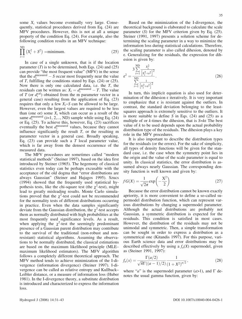
The MFV procedures may be facilitated for manyproblems in hydrogeology. Figure 3 shows an example ofa simple linear fitting of the water level data derived froma thick Pleistocene aquifer. Water levels were measuredin two different wells, where there was a strong correla-tion between the levels because of hydraulic communi-cation between the screened layers. This strong relation-ship was also given by the generalized and robust corre-lation factor (Steiner 1997). Although it was derived fromthe traditional Pearson correlation coefficient, the gener-alized correlation factor has also a robust and resistantbehavior. The traditional (Pearson-type) linear correlationfactor showed only a weak relationship due to presence ofthe outliers. Figure 3 indicates that the linear relationshipbased on the least-squares principle can be heavily in-fluenced by the presence of outliers (produced artificiallyby human error in this case). Whereas, the MFV proce-dure clearly avoids the misleading bunch of data andprovides a realistic linear physical relationship instead ofa statistically distorted one. For the MFV fitting, thefollowing expression was minimized by the SA method toderive the values of the fitting parameters (a and b) for thelinear regression equation.

P2 ¼ eYND

i¼1

1þh2;i � ah1;i þ b

� �� �2

2eð Þ2

!" #1=2 ND

; ð44Þ

where h1,i and h2,i values are the measured water levels inwells #1 and #2, respectively.

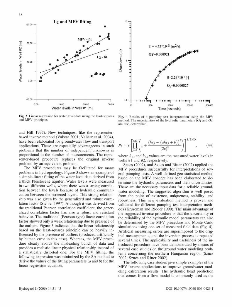
Szucs (2002), and Szucs and Ritter (2002) applied theMFV procedures successfully for interpretations of sev-eral pumping tests. A well-defined geo-statistical methodbased on the MFV concept has been elaborated to de-termine the hydraulic parameters and their uncertainties.These are the necessary input data for a reliable ground-water modeling. The suggested algorithm is well posedfrom the point of existence, uniqueness, stability, androbustness. This new evaluation method is proven andvalidated for different pumping test interpretation meth-ods (Kruseman and Ridder 1990). The main advantage ofthe suggested inverse procedure is that the uncertainty orthe reliability of the hydraulic model parameters can alsobe determined by the MFV procedure and Monte Carlosimulations using one set of measured field data (Fig. 4).Artificial measuring errors are superimposed to the orig-inal measurements, and the inversion process is repeatedseveral times. The applicability and usefulness of the in-troduced procedure have been demonstrated by means ofseveral case studies on the ground water modeling prob-lems concerning the northern Hungarian region (Szucs2002; Szucs and Ritter 2002).

The following case studies give simple examples of theMFV inverse applications to improve groundwater mod-eling calibration results. The hydraulic head predictionthat comes from a flow model is commonly used as the

Fig. 3 Linear regression for water level data using the least-squaresand MFV principles

Fig. 4 Results of a pumping test interpretation using the MFVmethod. The uncertainties of the hydraulic parameters (QT and QS)are also determined

38

Hydrogeol J (2006) 14:31–43 DOI 10.1007/s10040-004-0426-1

basis for model calibration. Calibration is a process ofadjusting the model parameters to achieve a satisfactorymatch between the predicted (or calculated) and measuredhydraulic heads (Hill 1998). Practically, calibration is aninverse process. Most commonly, calibration is accom-plished by a trial-and-error adjustment of the model pa-rameters based on the expert experience to achieve thebest match between the measured and calculated data.The calibration based on the above-mentioned mathe-matical approaches is referred to as the automated inverseprocedures in groundwater modeling (Hill 1992). Fre-quently, the objective function used as a calibration cri-terion is based on the mean error, the mean-absolute error(L1 norm), or the root-mean-square error (RMS error, L2norm) (Anderson and Woessner 1992). Concerning thehydraulic heads (h), the RMS error can be defined as:

RMSE ¼ 1ND

XND

i¼1

hmeasuredi � hcalculated

i

� �2

" #0:5

: ð45Þ

Szucs and Ritter (2002) introduced the above-men-tioned Pk-norm for groundwater model calibration pur-poses. Because the real data, and the error or residualdistribution can never be known in advance, the usage ofPk=2-norm is most favorable for groundwater modeling.The definition of the Pk=2-norm is given based on above-mentioned theory as:

Pk¼2 ¼ eYND

i¼1

1þhmeasured

i � hcali

� �2

2eð Þ2

!" #1=2 ND

: ð46Þ

To demonstrate the advantage of the MFV procedureand global optimization in groundwater modeling, twomain examples are provided here. First, the above-de-scribed methodology is tested and verified by means ofthe synthetic data of a predefined groundwater model.Then, a practical wellhead protection zone delineationexample is carried out in order to illustrate the applicationof the suggested method.

Test problemA simple one-layer unconfined steady-state groundwatermodel has been facilitated to describe and investigate thebehavior of the proposed global optimization (SA)method and the MFV procedure. The x–y dimension ofthe test model is 1 km by 1 km. The top of the model layeris on 25 m. The bottom of the model layer is 0.0 m. Thebasic grid size is 20 m. A constant recharge rate at0.0003 m3/(m2 day) was applied on the top of the gridsystem. Four polygons were delineated to represent thelayer heterogeneity in the aquifer. The horizontal hy-draulic conductivity is assumed to be constant in eachpolygon. Specified head boundary conditions were in-troduced on the west and east borders to simulate thenatural groundwater flow from west to east. One pro-duction well was seated in each of polygon I (�400 m3/s),II (�500 m3/s) and III (�300 m3/s). There is no well inpolygon IV. As over-determined systems are preferred forany statistical interpretation, 12 observation points were

stationed in the model for the groundwater calibration. Asa general working frame, the Groundwater ModelingSystem 4.0 package (EMRL 2002) was applied for thetest problem investigation. The flow model has beencreated with the help of the MODFLOW-2000 package(Harbough et al. 2000) using the prescribed model pa-rameters.

Creating a flow model based on the actual model pa-rameters is called a forward solution. The water levelscould be derived exactly for the 12 observation points. Tosimulate real measured water level data at the observationpoints, 2% random geostatistical error was superimposedon the exact water levels. Having a pre-defined hydro-geological model and the “measured data set,” the inverseinvestigations could be started. The GMS 4.0 systemprovides three built-in possibilities for automated inverseparameter estimation. These are the PEST (Doherty2000), the UCODE (Poeter and Hill 1998), and theMODFLOW-2000 PES (Hill et al. 2000) procedures.They are similar in effectiveness and all of them are basedon the classical statistical approaches. The MODFLOW-2000 PES method has been selected for comparison of theinvestigations with the present MFV based inverse algo-rithm using a global (metropolis simulated annealing)optimization (noted as MFV–SA). The MFV–SA inversemethod has been also linked to the popular MODFLOW-2000 package, which provides the forward solution. Inaddition to the well-described error functions (RMSE andP-norm), the relative model distance (RM) given byEq. (47) has also been used to characterize the accuracy ofthe compared inversion procedures.

RM ¼ 1NM

XNM

i¼1

m0i � mi

m0i

� �2 !1=2

; ð47Þ

where NM is the number of model parameters (NM=4 inthe present case), m0

i is the value of the i-th true modelparameter (hydraulic conductivities in the present testcase), mi is the i-th model parameter estimated based onthe actual inverse procedure. In synthetic investigations,the relative model distance can also be used because thepredefined model is known. Whereas in actual inversionsinvolving the field problems, this useful parameter cannotbe calculated, because the true model parameter valuesare never known exactly.

The present application of the MFV procedure utilizedthe classical simulated annealing global optimizationsearch, because there were only four model parameters.However, for large-scale groundwater models, the appli-cation of the VFSA is recommended to reduce the com-puter running time. For illustration, the metropolis (SA)algorithm was applied with the parameter values given asfollows. The initial temperature is T0=1.0. The finaltemperature is Tf=0.0001. The temperature reductionconstant is a=0.975. The number of iterations at eachtemperature is R(t)=300. Table 1 gives a summary of themost important results obtained by the MODFLOW-2000PES and MFV+SA algorithms. The results clearly indi-

39

Hydrogeol J (2006) 14:31–43 DOI 10.1007/s10040-004-0426-1

cate a great difference in the relative model distance (RM)values although the objective function values (RMSE andP-norm) are not far from each other. The relative modeldistance (RM=0.58, MODFLOW-2000 PES) reduces byhalf when the MFV based inverse procedure is applied(RM=0.27). Figures 5 and 6 also indicate the advantage ofthe MFV approach. Figure 5 shows nearly the same flowpattern as that of the original model. Figure 6 reflects thegeneral trends of the original model, but it involves manymore disturbances. The four polygons, where the hy-draulic conductivity values are different, can also be seenon Figs. 5 and 6. Note that even the MFV–SA method wasnot able to give back the original model parameters. Thisis truly understandable because a complication ingroundwater problems arises when the information aboutthe head distributions is incomplete (Anderson andWoessner 1992). In this example, only 12 “observed data”are present. Therefore, it is important to appreciate andconsider every piece of information concerning the heads.Hence, the statistical methods with high efficiency shouldbe used during the interpretation.

Field problemIn general, the field experts prefer to use the commer-cially available professional groundwater modelingpackages for hydrogeological evaluation and interpreta-tion, such as the above-mentioned Groundwater ModelingSystem (GMS 4.0) or the Processing Modflow (Chiangand Kinzelbach 2001). Although these packages havebuilt-in inverse modules like PEST, UCODE or MOD-FLOW-2000 PES, the trial-and-error calibration is stillpreferred in many cases because the modeler’s expertiseand experience can be involved in the process easily. Inthe following, the advantage of the MFV-based inversegroundwater modeling is demonstrated by a field exam-ple. Creating an inverse modeling program is not an easytask because it is difficult to incorporate the present im-proved subroutine to the existing standard groundwatermodeling packages. Nevertheless, the following exampledemonstrates how easily and advantageously the MFVprocedure can be applied to improve the interpretationresults even in the case of traditional trial-and-error cal-ibration.

Table 1 The main results of theinverse procedures carried outby MODFLOW-2000 PES andMFV–SA methods in case of2% geostatistical distributionerror added to the theoreticalheads at the observation points

Test problem investigated by different inversion methods

Model polygon Prescribed modelparameters

Model parameters from inversion

MODFLOW-2000 PES MFV–SA

I 25 m/day 11.52 m/day 18.72 m/dayII 35 m/day 27.65 m/day 32.14 m/dayIII 15 m/day 6.46 m/day 10.92 m/dayIV 10 m/day 1.90 m/day 7.38 m/dayError function RMSE=0.203 m P-norm = 0.172 mRelative model distance RM=0.58 RM=0.27

Fig. 5 Water levels in the flow model obtained using the mostfrequent value inverse procedure

Fig. 6 Water levels in the flow model obtained using the MOD-FLOW-2000 PES inverse procedure

40

Hydrogeol J (2006) 14:31–43 DOI 10.1007/s10040-004-0426-1

There is an ongoing national project supported by theHungarian government to delineate the wellhead protec-tion zones for vulnerable groundwater resources. Theparticle tracking MODPATH module (Pollock 1994) en-ables the delineation of the wellhead protection zonesaround the investigated production wells. Using themeasured and calculated water level data at the observa-tion points during the calibration process, the elements ofthe residuals can be determined as:

Xi ¼ dmeasuredi � dcal

i : ð48ÞBased on Eqs. (34), (35), (36), the most frequent value

(T) and the dihesion parameter of the head residuals canbe derived readily by means of a double-iteration process.Then, the MFV weights can be computed for each ob-servation point as:

Wi Xið Þ ¼keð Þ2

keð Þ2þ Xi � Tð Þ2: ð49Þ

Because the type of the residual distribution is notknown, the value of k=2 is preferred as discussed previ-ously. During each step of the trial-end-error calibration,the MFV weights can provide very visible and usefulinformation for every observation point about the actualgroundwater model condition concerning the strength ofmatching. The closer the MFV weight is to 1.0, the betterthe match between the measured and calculated head datafor the actual observation points. Besides the individualweight interpretation, the histogram of the MFV weightscan also give useful insight about the state of calibration.Figure 7 shows that the histogram has high relative fre-quency values at small MFV weights during the begin-

ning of the calibration when the model parameter valuesare far from their real values. The right histogram issignificantly different from the left one. This was ob-tained at the end of the trial-end-error calibration. If thecalibration is carried out successfully and the measureddata are reliable, the histogram should reflect highly onthe relative frequency at the greater intervals of MFVweights. In this way, the MFV weights derived from theresiduals can easily accelerate the trial-and-error process.

Conclusions

It has been demonstrated that the MFV method can beapplied successfully for effective solution of variousproblems involving groundwater modeling under certainconditions, such as when the measurement errors are notGaussian and the model concept errors are insignificant.This robust and resistant geostatistical procedure providesa high general efficiency. Well-posed and over-deter-mined inverse problems investigated in this paper havedemonstrated the usefulness of the MFV algorithms.

The application of the P-norms based on the MFVprinciple has been shown to be advantageous over theother types for inverse parameter estimation calculations.The automated parameter estimation method facilitatingthe MFV method and linked to the MODFLOW-2000-reference flow code has been shown to be effective forderiving the groundwater model parameters. The use ofthe MFV weights of the head residuals readily improvesthe groundwater interpretation results during traditionaltrail-and-error calibration processes. The VFSA opti-mization method has been shown to be reliable without

Fig. 7 Histograms of the MVF weights during the calibration process. The left histogram (a) shows an early stage and the right histogram(b) reflects the end of the trial-end error calibration

41

Hydrogeol J (2006) 14:31–43 DOI 10.1007/s10040-004-0426-1

requiring the initial guess of the model parameter valuesto be sufficiently close to the actual values.

The present study has proven that the MFV methodprovides certain advantages over the conventional statis-tical methods derived from the maximum likelihoodprinciple. Consequently, the application of the MFVmethod coupled with global optimization is expected tobecome a more widespread practice in groundwatermodeling. However, the proposed method is not a remedyfor ill-posed groundwater modeling problems. Also, theslightly high computational effort requirement of theMFV method may be a drawback. Further improvementsand refinements are recommended for future studies inorder to make the MFV method much more versatile forgroundwater modeling applications.

Acknowledgements The authors gratefully acknowledge the Ful-bright Scholarship Program, the Bolyai Janos Research Scholarshipof the Hungarian Academy of Sciences, and the Mewbourne Schoolof Petroleum and Geological Engineering at the University ofOklahoma for support of this work

References

Anderson MP, Woessner WW (1992) Applied ground-water mod-eling. Academic, San Diego, CA, 381 pp

Carrera J, Neuman SP (1986a) Estimation of aquifer parametersunder transient and steady state conditions. 1. Maximum like-lihood method incorporating prior information. Water ResourRes 22(2):199–210

Carrera J, Neuman SP (1986b) Estimation of aquifer parametersunder transient and steady state conditions. 2. Uniqueness,stability and pollution algorithms. Water Resour Res22(2):211–227

Carrera J, Neuman SP (1986c) Estimation of aquifer parametersunder transient and steady state conditions. 3. Application tosynthetic and field data. Water Resour Res 22(2):228–242

Chiang WH, Kinzelbach W (2001) 3D-Groundwater modeling withPMWIN. A simulation system for modeling groundwater flowand pollution. Springer, Berlin Heidelberg New York, 346 pp

de Marsily Gh, Delhomme JP, Coundrain-Ribstein A, Lavenue AM(2000) Four decades of inverse problems in hydrogeology. Parudans Geophysical Society of America, Special paper 348:1–28

Dobr�ka M, Gyulai �, Ormos T, Csok�s J, Dresen L (1991) Jointinversion of seismic and geoelectric data recorded in an un-derground coal mine. Geophys Prospect 39:643–665

Doherty J (2000) PEST, model-independent parameter estimation,4th edn. program documentation. Watermark NumericalComputing, p 249

Dutter R (1987) Mathematische Methoden in der Montangeologie.Vor-lesungsnotizen, Manuscript, Leoben

EMRL, Environmental Modeling Research Laboratory of BrighamYoung University (2002) Groundwater modeling system (GMS4.0), Tutorial manual

Ferenczy L, Kormos L, Szucs P (1990) A new statistical method inwell log interpretation, paper O. In: 13th European formationevaluation symposium transactions: Soc. Prof. Well Log Ana-lysts, Budapest Chapter, 17 pp

Hajagos B, Steiner F (1991) Different measures of the uncertainty.Acta Geod Geophys Montan Hung 26:183–189

Hajagos B, Steiner F (1995) Symmetrical stable probability dis-tributions nearest lying to the types of the supermodel fa(x).Acta Geod Geophys Hung 30(2–4):463–470

Harbaugh AW, Banta ER, Hill MC, McDonald MG (2000)MODFLOW-2000, The U.S. Geological Survey modularground-water model—user guide to modularization concepts

and the ground water flow process. U.S. Geological Survey,Open-file report 00–92

Hill MC (1992) A computer program (MODFLOWP) for estimat-ing parameters of a transient, three-dimensional ground waterflow model using nonlinear regression. U.S. Geological Survey,Open-file report 91–484

Hill MC (1998) Methods and guidelines for effective model cali-bration. U.S. Geological Survey, Water-resources investiga-tions report 98-4005

Hill MC, Banta ER, Harbaugh AW, Anderman ER (2000) MOD-FLOW-2000, The U.S. Geological Survey modular ground-water model—user guide to the observation, sensitivity, andparameter-estimation processes and three post-processing pro-grams. U.S. Geological Survey, Open-file report 00-184

Huber PJ (1981) Robust statistics. Wiley, New York, 308 ppIngber L (1989) Very fast simulated reannealing. Math Comput

Modeling 12(8):967–993Isaaks EH, Srivastava RM (1989) Applied geostatistics. Oxford

University Press, Oxford, pp 1–561Kirkpatrick S, Gelatt CD Jr, Vecchi MP (1983) Optimization by

simulated annealing. Science 220:671–680Kitandis PK (1997) Introduction to geostatistics: applications to

hydrogeology. Cambridge University Press, Cambridge, 249 ppKruseman GP, de Ridder NA (1990) Analysis and interpretation of

pumping test data, Publication 47. International Intsitute forLand Reclamation and Improvement, Wageningen, The Nether--lands, pp 1–375

Lebbe LC (1999) Hydraulic parameter identification. Generalizedinterpretation method for single and multiple pumping tests.Springer, Berlin Heidelberg New York, 359 pp

Lee T-C (1999) Applied mathematics in hydrogeology. CRC Press,Boca Raton, FL (ISBN 1-56670-375-1)

Lines TR, Treitel S (1984) Tutorial: a review of least squares in-version and its application to geophysical problems. GeophysProspect 32:159–186

Marquardt DW (1970) Generalized inverses, Ridge regression, bi-ased linear estimation, and nonlinear estimation. Techometrics12:591–612

Menke W (1984) Geophysical data analysis: discrete inverse the-ory. Academic, San Diego, CA

Metropolis N, Rosenbluth A, Rosenbluth M, Teller A, Teller E(1953) Equations of state calculations by fast computing ma-chines. J Chem Phys 21:1087–1092

Poeter EP, Hill MC (1997) Inverse models: a necessary next step ingroundwater modeling. Ground Water 35(2):250–260

Poeter EP, Hill MC (1998) Documentation of UCODE. A computercode for universal inverse modeling. U.S. Geological Survey,Water-resources investigations report 98–4080

Pollock DW (1994) User’s guide for MODPATH/MODPATH-PLOT, version 3: a particle tracking post-processing packagefor MODFLOW, the U.S. Geological Survey finite differenceground-water flow model: U.S. Geological Survey open-filereport 94-464, 6 ch

Sen M, Stoffa PL (1995) Global optimization methods in geo-physical inversion. Elsevier, Amsterdam, The Netherlands. AdvExplor Geophys 4

Steiner F (1965) Interpretation of Bouguer-maps (in Hungarian).Dissertation, Manuscript, Miskolc, pp 80–94

Steiner F (1972) Simultane interpretation geophysikalischer mess-datensysteme. Rev Pure Appl Geophys 96:15–27

Steiner F (1988) The most frequent value procedures. GeophysTrans 34(2–3):226

Steiner F (1990) The bases of geostatistics (in Hungarian).Tankonyvkiado, Budapest, Hungary, 363 pp

Steiner F (ed) (1991) The most frequent value. Introduction to amodern conception statistics. Akademia Kiado, Budapest,Hungary, 314 pp

Steiner F (ed) (1997) Optimum methods in statistics. AkademiaKiado, Budapest, Hungary

Steiner F, Hajagos B (1994) Practical definition of robustness.Geophys Trans 38:193–210

42

Hydrogeol J (2006) 14:31–43 DOI 10.1007/s10040-004-0426-1

Steiner F, Hajagos B (1995) Determination of the parameter errors(demonstrated on a gravimetric example) if the geophysicalinversion is carried out as the global minimization of arbitrarynorms (demonstrated by the Pc norm). Magyar Geofizika36:261–276

Sun N-Z (1994) Inverse problems in groundwater modeling.Kluwer, Dordrecht

Szucs P (1994) Comment on an old dogma: ‘the data are normallydistributed’. Geophys Trans 38:231–238

Szucs P (2002) Inversion of pumping test data for improved in-terpretation. In: microCAD 2002, International scientific con-ference, University of Miskolc, A: Geoinformatics, 7–8 March2002, pp 107–112

Szucs P, Civan F (1996) Multi-layer well log interpretation usingthe simulated annealing method. J Pet Sci Eng 14:209–220

Szucs P, Ritter Gy (2002) Improved interpretation of pumping testresults using simulated annealing optimization. In: Model-CARE 2002, Proceedings of the 4th international conference oncalibration and reliability in groundwater modeling, Prague,Czech Republic, 17–20 June 2002. Acta Universitas Carolinae– Geologica 2002, 46(2/3):238–241

T�th J (1999) Groundwater as a geologic agent: An overview of thecauses, processes, and manifestations. Hydrogeol J 7:1–14

Valstar JR (2001) Inverse modeling of groundwater flow andtransport. PhD thesis, Delft University of Technology

Valstar JR, McLaughlin DB, te Stroet CBM, van Geer FC (2004)The representer-based inverse method for groundwater flowand transport applications. Water Resour Res 40:W05116. DOI10.1029/2003WR002922

43

Hydrogeol J (2006) 14:31–43 DOI 10.1007/s10040-004-0426-1