appendix - university of alberta
TRANSCRIPT
Appendix
1 Linear Algebra
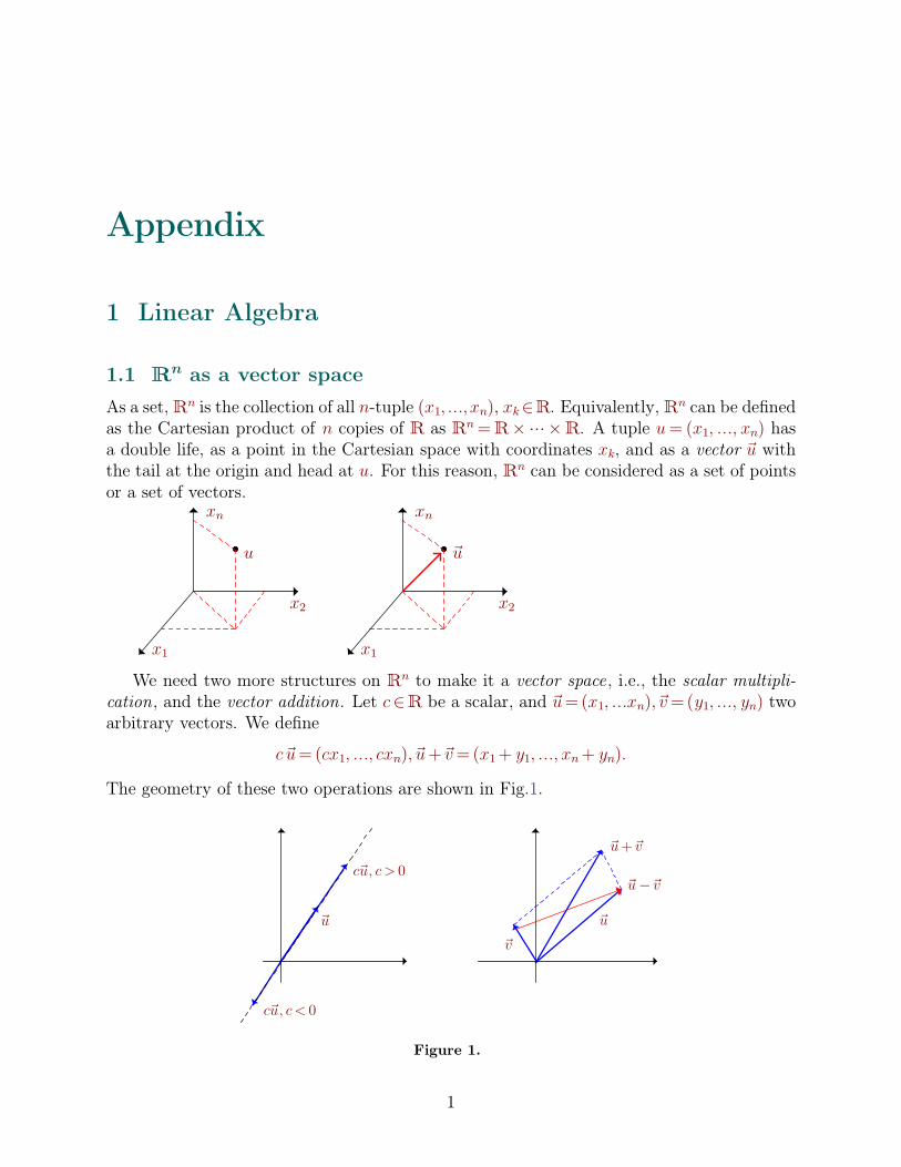
1.1 Rn as a vector spaceAs a set,Rn is the collection of all n-tuple (x1; :::;xn), xk2R. Equivalently,Rn can be definedas the Cartesian product of n copies of R as Rn=R� ��� �R. A tuple u= (x1; :::; xn) hasa double life, as a point in the Cartesian space with coordinates xk, and as a vector u~ withthe tail at the origin and head at u. For this reason, Rn can be considered as a set of pointsor a set of vectors.
u
x1
xn
x2 x2
xn
u~
x1
We need two more structures on Rn to make it a vector space, i.e., the scalar multipli-cation, and the vector addition. Let c2R be a scalar, and u~ =(x1; :::xn); v~ =(y1; :::; yn) twoarbitrary vectors. We define
c u~ =(cx1; :::; cxn); u~ + v~ =(x1+ y1; :::; xn+ yn):
The geometry of these two operations are shown in Fig.1.
cu~ ; c< 0
u~
cu~ ; c> 0
v~
u~ + v~
u~ ¡ v~
u~
Figure 1.
1

It is seen that Rn is closed under the defined operations, that is, for any two vectors u~ ;v~ in Rn, and c1; c22R, vector c1u~ + c2v~ is in Rn. Moreover, the following properties hold forany vectors u~ ; v~ ;w~ 2Rn and constant c2R:
i. u~ + v~ = v~ +u~
ii. c (u~ + v~)= c u~ + c v~
iii. (c1+ c2)u~ = c1u~ + c2u~
iv. (u~ + v~)+w~ =u~ +(v~ +w~ )
Rn has n standard unit vectors e1; :::; en defined below
e1=
0BBBBBB@10���0
1CCCCCCA; e2=0BBBBBB@
01���0
1CCCCCCA; :::; en=0BBBBBB@
00���1
1CCCCCCA:The set fekgk=1n is a basis for Rn in the sense that any vector u~ =(x1; :::; xn) can be uniquelyrepresented as
u~ =x1 e1+ ���+xn en:
Remark. The magnitude or norm of a vector u~ =(x1; :::; xn) is defined as follows
ku~ k=Xk=1
n
xk2
s:
A vector is called unit or a direction vector if its norm is equal 1. We usually denote unitvector by notation ^.
1.2 Dot and Cross productsThe dot product of two arbitrary vectors u~ =(x1; :::; xn); v~ =(y1; :::; yn) is defined as
u~ � v~ =Xk=1
n
xi yi:
In particular, ei � ej= �i;j where �i;j=�1 i= j0 i=/ j
.
Problem 1. Show that the dot product enjoys the following properties for any vectors u~ ; v~ ; w~ and forarbitrary constant c
i. (u~ + v~) �w~ =u~ �w~ + v~ �w~ ,ii. u~ � v~ = v~ �u~ ,iii. (c u~ ) � v~ = c (u~ � v~)
Problem 2. Show the following relations
a) ku~ k2=u~ �u~b) ku~ + v~k�ku~ k+ kv~ kc) ku~ + v~k2¡ku~ ¡ v~k2=4 u~ � v~
Problem 3. The Cauchy inequality is as follows
u~ � v~ �ku~ k kv~k:
2 Appendix

Try to prove the inequality by the following method: ku~ + t v~k2� 0 for all t 2R. Expand ku~ + t v~k2 interms of t and conclude the inequality. By this inequality, one can define the angle between two nonzerovectors u~ ; v~ as follows
cos(�)= u~ � v~ku~ k kv~k :
By the above equality, one can write (u~ ; v~) = ku~ k kv~k cos(�). Note that if u~ � v~ =0 for non-zero vectorsu~ ; v~ , then cos(�)= 0.
Problem 4. Show that if u~ 1; :::; u~m are mutually orthogonal, that is, if u~ i �u~ j=0 for i=/ j then
ku~ 1+ ���+u~mk2= ku~ 1k+ ���+ ku~mk2:
There is a standard product in R3 called cross or external product . For u~ = (x1; y1; z1);v~ =(x2; y2; z2), the cross product is defined as follows
u~ � v~ =
������������e1 e2 e3x1 y1 z1x2 y2 z2
������������=(y1z2¡ z1y2)e1+(z1x2¡x1z2)e2+(x1y2¡ y1x2)e3:
Note that u~ � v~ is a vector, while their dot product is a scalar.Problem 5. Show the relation u~ � v~ =¡v~ �u~ .Problem 6. Show that u~ � v~ is perpendicular to u~ and v~ , that is,
(u~ � v~) �u~ =(u~ � v~) � v~ =0:Problem 7. Show the identity
ku~ � v~k2= ku~ k2ku~ k2¡ ju~ � v~ j2;and conclude the relation
ku~ � v~k= ku~ k kv~k sin(�);
where � is the angle between u~ ; v~ in [0; �].
By the above problem, we can write
u~ � v~ = ku~ k kv~k sin(�) n;
where n is the unit vector perpendicular to the plane containing u~ ; v~ , that is, n= u~ � v~ku~ � v~k .
A= jju~ � v~ jj
�
u~ � v~
u~ v~A
v~ �u~
Problem 8. Show the following relation for any three vectors u~ ; v~ ; w~
u~ � (v~ �w~ )= v~ � (w~ �u~ ):
Problem 9. If v~ ; w~ are orthogonal, show the following relation
u~ � (v~ �w~ )= (u~ �w~ )v~ ¡ (u~ � v~)w~ :
Use this result and relax the condition v~ ; w~ to be orthogonal. Use the formula and determine theconditions the following relation holds
u~ � (v~ �w~ )= (u~ � v~)�w~ :
1 Linear Algebra 3
1.3 Subspaces and direct sum
Definition 1. Tow vectors u~ ; v~ in Rn are called linearly dependent if there is a scalar csuch that u~ = c v~ or v~ = c u~ . A vector u~ is linearly dependent on vectors v~1; :::; v~m if there arescalars c1; :::; cm such that
u~ = c1v1~ + ���+ cmv~m:
Vectors v~1; :::; v~m in Rn are linearly independent if the linear combination
c1 v~1+ ���+ cm v~m=0;
implies c1= ���= cm=0.
Problem 10. Vectors e1; :::; en are linearly independent in Rn. Show that any n+1 vectors of Rn arelinearly dependent.
Let fv~1; :::; v~dg for d � n be a set of linearly independent vectors in Rn. The span ofvectors in the given set is the set of all possible linear combinations of v~1; :::; v~d, i.e.,
spanfv~1; :::; v~dg= fc1v~1+ ���+ cd v~d; ck2Rg:
Note that Rn is itself equal to spanfe1; :::; eng.
Proposition 1. Vd := spanfv~1; :::; v~dg is closed under the vector addition and scalar multi-plication of Rn. For this reason, Vd is called a linear subspace of Rn.
Definition 2. Let V be a linear subspace of Rn. The dimension of V is the maximumnumber of linearly independent vectors in V.
Example 1. Technically speaking, Rm is not a subspace of Rn for m < n, however, if weinterpret Rm as spanfe1; :::; emg where each ej is a vector in Rn, then Rm is a linear subspaceof Rn.
If V is a linear subspaces of Rn, then its orthogonal subspace V? is defined as follows
V?= fw~ 2Rn;w~ � v~ =0; v~ 2Vg:
Obviously, V? is a linear subspace of Rn equipped with the vector addition and scalarmultiplication operations.
Problem 11. Show that ifV= spanf(1;1;0); (0;1;1)g, thenV? is the one dimensional subspace spannedby (1;¡1; 1).
Problem 12. Find the orthogonal subspace of V= f(1; 0; 1)g in R3.
Suppose U;V are two subspaces of Rn and U\V=f0g. The direct sum U�V is definedas follows
U�V= fc1u~ + c2v~ ; u~ 2U; v~ 2Vg:
Problem 13. If V is a subspace of Rn, show that Rn=V�V?.
Problem 14. Let V be an arbitrary subspace of Rn. Show that every vector u~ in Rn can be representeduniquely as u~ = c1v~ + c2w~ for v~ 2V and w~ 2V?.
4 Appendix

1.4 Matrices and linear mappings
Definition 3. A mapping f :Rn!Rm is called linear if for any constants c1; c2 and anyvectors u~ ; v~ 2Rn, the following relation holds
f(c1u~ + c2 v~)= c1f(u~ )+ c2f(v~):
Problem 15. If f :Rn!Rm is linear then f(0)= 0.
Proposition 2. A linear mapping f :Rn!Rm can be represented by a m�n matrix.
Proof. Remember that a matrix A=[aij]m�n is a structure of n-columns of vectors belongingRm, i.e., A = [A1j���jAn], where Ak 2 Rm. The action of A to ek is defined by the relationA (ek)=Ak. Now define Af as
Af = [f(e1)jf(e2)j���jf(en)]:
It is simply seen that for arbitrary vector u~ 2Rn, the following relation holds f(u~ )=Af(u~ ). �
Problem 16. Let T :R2!R2 has the matrix representation A2�2=�1 10 1
�in the standard basis. Find
the matrix representation of T in the basis v~1=�11
�; v~2=
�1¡1
�.
Problem 17. Prove that a matrix 2� 2 maps any parallelogram to a parallelogram.
Problem 18. Verify that the the matrix R�=�
cos(�) ¡sin(�)sin(�) cos(�)
�rotates vectors in the plane by � degree
counter-clockwise. Verify that R�1R�2=R�1+�2 and conclude that R�R¡� is the identity matrix�1 00 1
�.
Definition 4. Let f :Rn!Rm be a linear mapping. The kernel (or null space) of f, denotedby ker(f) (or just Nf) is a set of all vectors n~ of Rn such that f(n~ ) = 02Rm. The imageof f denoted by Im(f) is the set of all vectors w~ 2Rm such that w~ = f(v~) for some v~ 2Rn.
Proposition 3. The kernel of a linear mapping f : Rn! Rm is a vector subspace of Rn.The image of f is a vector subspace of Rm.
Problem 19. Prove the proposition.
Theorem 1. Assume that f :Rn!Rm is a linear mapping. The following relation holds
n=dimker(f)+dim Im(f): (1)
Problem 20. Let S denote the orthogonal subspace of ker(f). Show that dim S = dim Im(f) andconclude f(S)= Im(f).
1.5 Linear mappings from Rn to Rn
1.5.1 Determinant
Let f :Rn!Rn be a linear mapping, and let C be a unit cube constructed on ek; k=1; :::;n. The image of C under f , that is f(C), is a parallelogram. In fact, every vector u~ 2C isrepresented by the linear combination
u~ = c1e1+ ���+ cn en;
1 Linear Algebra 5

for 0� ck� 1, and thus
f(u~ )= c1f1~ + ���+ cn fn~ ;
where fk= f(ek). The set fc1f1~ + ���+ cn fn~ g for 0� ck� 1 is a parallelogram constructed onf1~ ; :::; f~n; see Fig. 2 .
e1
f~1= f(e1)f~2= f(e2)
e2
Figure 2.
Definition 5. Let f :Rn!Rn be a linear mapping, and let C be the unit cube constructedon fekgk=1n . The determinant of f denoted by det(f) is the algebraic volume of parallelogramf(C). The algebraic volume is the signed volume with positive or negative signs.
Example 2. In R2, the determinant of A=�a11 a12a21 a22
�is defined by the following formula
det�a11 a12a21 a22
�= a11a22¡ a12a21: (2)
It is simply verified that jdet(A)j= jjA(e1)jj jjA(e2)jj sin(�), where � is the angel between twocolumns of A.
If det(f) = 0, then the volume degenerates, that means vectors f~1; :::; f~n are linearlydependent. If det(f) < 0, then f changes the standard orientation of the basis fekgk=1n
(remember the standard rotations inR2 andR3), for example f(x; y)=(y;x) with the matrixrepresentation
A= [f(e1)jf(e2)] =�0 11 0
�;
changes the standard rotation. Let Af = [f~1j���jf~n] be the representation of f :Rn!Rn inthe standard basis fekgk=1n . The determinant det(Af) satisfies the following properties:
i. If f1~ ; ���; f~n are linearly dependent then det[A] = 0
ii. det[f~2jf~1j���jfn~ ] = ¡det[Af]. In general any switch between column i and j multiplethe determinant by the factor (¡1)i+j.
iii. det[c f~1jf2~ j���jfn~ ] = cdet(Af)
iv. det[c1f~1+ c2f~kjf~2j���jf~n] = c1 det[Af] for any k=2; :::; n.
By the above properties, it is seen that if f ; g:Rn!Rn are two linear mappings then
det(AB)= det(A) det(B)
6 Appendix

Problem 21. Verify directly the above claim for 2� 2 matrices.
1.5.2 Injective and surjective mappings
Definition 6. A linear mapping f : Rn! Rm is called one-to-one or injective if equalityf(u~ ) = f(v~) implies u~ = v~. A linear mapping f : Rn! Rm is called onto or surjective, ifRm= f(Rn).
Problem 22. A linear mapping f :Rn!Rn is one to one if and only if ker(f) = ;, and if and only ifit is onto.
Problem 23. Let f :Rn!Rm be a linear mapping. Show that if m > n, then f can not be onto, ifm<n then f can not be one-to-one.
If f :Rn!Rn is one-to-one (and then onto), the mapping f¡1: Rn!Rn is called theinverse mapping of f if the following relation holds
ff¡1= f¡1f = Id;
where Id is the identity mapping on Rn. The identity mapping has the matrix representationdiag(1; :::;1), where diag(1; :::; 1) has 1 on the main diagonal and zero everywhere else. Notethat Id(u~ )= u~ for any vector u~ .
Problem 24. If f :Rn!Rn is a one to one linear map, show that f¡1 is also a one to one linear map.
1.5.3 Eigenvalues and Eigenvectors
A vector v~ 2Rn ¡ f0g is called an eigenvector of a linear mapping f :Rn!Rn if there isa scalar � such that f(v~) = �v~. It is seen that if v~ is an eigenvector, then vector w~ = tv~ forarbitrary scalar t is also an eigenvector. Accordingly, one can define an eigendirection of fthat is spanfv~ g := ft v~ ; t2Rg; see Fig. 3.
v~
�v~ = f(v~)
f
Figure 3.
Example 3. The vector v~ = (1; 1) is an eigenvector of the matrix A =�
1 1¡1 3
�with the
eigenvalue �=2, because�
1 1¡1 3
��11
�=2
�11
�. Matrix A=
�1 1¡1 3
�has only one eigenvector
and matrix A=�
2 3¡4 ¡5
�has two eigenvectors v~1=(1;¡1) and v2~ =(3;¡4) with eigenvalues
�1 = ¡1 and �2 = ¡2 respectively. The rotation matrix R� =�
cos(�) ¡sin(�)sin(�) cos(�)
�has no (real)
eigenvector for � =/ 0; 2�. Recall that R� rotates vectors counterclockwise by �-angle. Theidentity matrix I2�2=
�1 00 1
�has infinitely many eigenvectors. In fact, every vector in R2 is
an eigenvector of Id2�2 with eigenvalue �=1.
1 Linear Algebra 7

Proposition 4. If f : Rn! Rn has n distinct eigenvalues �1; :::; �n, then their associatedeigenvectors v~1; :::; v~n are linearly independent.
Problem 25. Prove the proposition.
If v~ is an eigenvector of a linear mapping f with eigenvalue �, then (f ¡�Id)v~ =0, andsince v~ is nonzero, v~ must belong to the kernel of f ¡�Id. Let Af is a matrix representationof f , then the following relation holds
det(Af ¡�Id)= 0:
The above equation, which is an algebraic equation of �, is called the characteristic equationof f . If A=
�a11 a12a21 a22
�, the characteristic equation is as follows
�2¡ tr(A)�+ det(A)=0; (3)
where tr(A) (read trace A) is equal to a11+ a22.
Problem 26. Show that if A2�2 has a repeated eigenvalue � with two linearly independent eigenvectorsthen all vectors of R2 is an eigenvector of A.
Problem 27. Let A be a 2� 2 matrix. Prove that the following statements are equivalent
i. A is invertible.
ii. Two columns of A are linearly independent.
iii. The determinant of A is non-zero.
iv. No eigenvalue of A is zero.
Problem 28. If �1; �2 are two eigenvalues of A2�2, show that det(A)=�1�2 and tr(A)=�1+�2.
Problem 29. If Q2�2 is an invertible matrix, show the following relations
tr(Q¡1AQ)= tr(A), det(Q¡1AQ)= det(A):
1.5.4 Symmetric mappings and Jordan forms
Definition 7. A linear mapping f : Rn! Rn is called symmetric if the following equalityholds for arbitrary vectors u~ ; v~ 2Rn:
f(u~ ) � v~ =u~ � f (v~):
Theorem 2. If the linear mapping f : Rn! Rn is symmetric, then there are n mutuallyorthogonal eigenvectors v~1; :::; v~n for f. Moreover, all eigenvalues of f are real.
Problem 30. Assume v~1; v~2 are two eigenvectors of a symmetric mapping f . Show that hv~1; v~2i=0.
If f : Rn ! Rn has n linearly independent eigenvectors v~1; :::; v~n, then Rn can bedecomposed by the direct sum Rn=V1�����Vn where Vk= spanfv~kg. The restriction of fto each Vk is a linear mapping fk:Vk!Vk, and thus we can decompose f as the direct sumf = f1� ��� � fn. With this interpretation, every vector v~ 2Rn has a unique representationv~ = c1 v~1+ ���+ cn v~n, and thus f(v~) is
f(v~)= f1(c1 v~1)+ ���+ fn(cn v~n)= c1�1 v~1+ ���+ cn�n v~n
8 Appendix

Definition 8. A linear mapping f : Rn! Rn is called positive definite if for any nonzerovector v~, the following inequality holds
f(v~) � v~ > 0:
A negative definite linear mapping is defined similarly.
It is simply seen that if Af = [aij] is the matrix representation of the positive definitemapping f in the standard basis, then aii> 0 for i=1; :::; n. Moreover, all real eigenvaluesof Af must be positive.
Problem 31. Let f :Rn!Rn be a symmetric mapping. A necessary and sufficient condition that f bepositive definite is that its all eigenvalues are positive.
If Qn�n is an invertible matrix, then two matrices B=Q¡1AQ and A are called similar .It is seen that A;B have same characteristic polynomial as the following argument justifies it:
det(Q¡1AQ¡ �Id)=detQ¡1(A¡�Id)Q=det(Q¡1)det(A¡�Id)detQ= det(A¡�Id):
Proposition 5. Suppose An�n has n linearly independent eigenvectors v~1; :::; v~n. Then thefollowing relation holds
Q¡1AQ=diag(�1; :::; �n);
where for Q= [v~1j���j v~n], and �1; :::; �n are associated eigenvalues (not necessarily distinct).Matrix diag(�1; :::; �n) is called the Jordan form of A.
Problem 32. Prove the above proposition.
Fig. 4 shows the relation between eigenvectors of A and Q¡1AQ .
Eigenvectors ofEigenvectors of A
v~1v~2
Q¡1AQ
e2~
e1~
Figure 4.
Problem 33. Let A=�¡4 ¡33 2
�. Find the matrix Q¡1AQ.
If a matrix An�n has n repeated eigenvalues � with only one eigenvector, then theJordan form of An�n is a diagonal matrix with � on the main diagonal and 1 on the upperdiagonal. For example, for a 3 � 3 matrix with repeated eigenvalue �, the Jordan form
is
0BB@ � 1 00 � 10 0 �
1CCA. If a matrix 2� 2 has two complex eigenvalues � = � � i!, its Jordan form is�� ¡!! �
�.
Problem 34. For a n�n matrix A show det(A)=Q
k=1n
�k, and conclude that A is one-to-one if andonly if A does not have a zero eigenvalue.
1 Linear Algebra 9

1.6 Linear equations
Let f : Rn! Rm be a linear mapping, and let b~ 2 Rm be an arbitrary vector. The linearequation f(u~ ) = b~ is solvable if and only if b~ 2 Im(f). If f :Rn!Rn is a linear one-to-onemapping, then equation f(u~ )= b~ is simply solved for u~ = f¡1(b~). If dimker(f)> 0 and u~ is asolution to the equation, then for any vector n~ 2 ker(f), v~ =n~ +u~ is also a solution. In thiscontext, vectors in ker(f) are called the homogeneous solutions of f(u~ )=0.
Problem 35. Suppose n�m and f :Rn!Rm is a linear mapping. Show that if dim ker(f) = n¡m,then the linear equation f(u~ )= b~ is solvable for any b~ 2Rm. What if dimker(f)>n¡m? If n>m anddimker(f)=n¡m, show that the equation f(u~ )= b~ has infinitely many solutions.
Problem 36. Let A=�2 61 3
�. For what values of b~ 2R2, the equation Au~ = b~ is solvable? Verify that
the solutions of the equation Au~ =�42
�has the form u~ = t
�¡31
�+
�20
�for t2 (¡1;1).
Problem 37. Let f :Rn!Rn be a linear mapping and let u1~ ;u~ 2 be two solutions to equation f(u~ )= b~.Show that u~ 1 ¡ u~ 2 2 ker(f), and conclude every solution to the equation can be represented by n~ + u~where n~ 2 ker(f).
Problem 38. Let f :Rn!Rn be a linear mapping and suppose u~ 1 is a solution to f(u~ )= b~1 and u~ 2 isa solution to f(u~ )= b~2. Show that u~ 1+u~ 2 is a solution to f(u~ )= b~1+ b~2.
As we saw above, equation f(u~ )=b~ is solvable if b~2 Im(f). The following problem answerthe solvability of a linear equation f(u~ )= b~ by the aid of the transpose of f . Remember thatf t:Rm!Rn is the transpose of f :Rn!Rm if the following equality holds for any u~ 2Rn,and v~ 2Rm
f(u~ ) � v~ =u~ � f t(v~):
Problem 39. Let f :Rn!Rm be a linear mapping. Show ker(f t)= [Im(f)]?. Conclude that the linearequation f(u~ )= b~ is solvable if hb~; n~ i=0 for all n~ 2 ker(f t). Also show
dimker(f t)¡dimker(f)=m¡n:
Problem 40. Find ker(f t) of the matrix A=�2 61 3
�and verify that b~=
�42
�is orthogonal to ker(f t).
2 Functions of several variables
2.1 Topology of Rn
For p=(x1; ���; xn)2Rn, the Euclidean norm kpk is defined as
kpk= x12+ ���+ xn
2p
;
and if q=(y1; :::; yn), the Euclidean distance is defined as follows
kp¡ qk= (x1¡ y1)2+ ���+(xn¡ yn)
2p
:
An immediate result of the above definitions is the convergence of sequences in Rn.
10 Appendix

Definition 9. A sequence (pm)m=11 is called convergent to a if
limm!1
kpm¡ ak=0:
Proposition 6. A sequence pm converges to a if and only if each coordinate of pm convergesto its associate coordinate of a.
An open ball of radius r centered at a2Rn is defined as
Br(a)= fp2Rn; kp¡ ak<rg:
a
r
Problem 41. If pn! a then any ball Br(a) contains infinitely many points of the sequence.
A set D�Rn is called open if for any point a 2D, there is r > 0 such that Br(a)�D.A set D�Rn is called bounded if there is r > 0 such that D�Br. If D is an open set thenits complement Dc is closed. The complement set Dc is defined as
Dc= fp2Rn; p2Dg:
If D is a set, its closure, cl(D) is the smallest closed set containing D, and bnd(D) denotesthe boundary set of D. A point a is called a boundary point of a set D if for any r > 0, thefollowing relation holds
Br(a)\D=/ ;; Br(a)\Dc=/ ;:
The above statements means that any ball centered at a crosses both D and Dc. We havebnd(Br)= fp; kpk= rg, and cl(Br)= fp; kpk� rg, and Br
c= fq; kqk>rg.
Problem 42. A set D�Rn is closed if and only if any convergent sequence (pn); pn2D converges in D.
Problem 43. Consider the set A=� 1n; n=1; 2; 3; ���
. Determine if A is open or closed.
Problem 44. Let D�Rn be any set, show that bnd(D) is closed.
Problem 45. Show that the set A=�y; 0< y<
1
x; x > 0
is open. Find bnd(A).
Problem 46. If D1; D2 are open sets show that D1[D2 and D1\D2 are open. Repeat the argumentif D1; D2 are closed.
2 Functions of several variables 11

2.2 Straight lines and planes in R3
The parametric equation of a straight line passing through a point p0 = (x0; y0; z0) andparallel to a vector r~ =(a; b; c) is p0~ + t r~ , or equivalently
x(t)=x0+ at; y(t)= y0+ bt; z(t)= z0+ ct:
If a=/ 0; b=/ 0; c=/ 0, then we can rewrite the equation as follows
x¡x0a
=y¡ y0b
=z¡ z0c
:
(p~ ¡ p0~ )jj r~
r~
p~ ¡ p0~
p0
p
Similarly, the equation of a straight plane in R3 passing through a given point p0=(x0;y0; z0), and perpendicular to a given vector n~ =(a; b; c) is n~ � (p~ ¡ p0~ )=0, or equivalently
a(x¡x0)+ b(y¡ y0)+ c(z¡ z0)= 0;
or equivalently ax+ by+ cz= d, for some constant d.
p0
p
p~ ¡ p~0
(p~ ¡ p0~ )?r~n~
The intersection of two planes in R3 can be empty or a line depending on their positionto each other. For example, two planes P1: a1x+ b1y + c1z = d1 and P2: a2x+ b2y + c2z = d2intersect if their normal vectors n~ 1= (a1; b1; c1) and n~ 2= (a2; b2; c2) are not parallel to eachother. In this case, the intersection line will be parallel to n~ 1�n~ 2
n~ 1�n~ 2=
��������������i j ka1 b1 c1a2 b2 c2
��������������=(b1c2¡ c1b2; c1a2¡ a1c2; a1b2¡ b1a2);
12 Appendix

Hence, the equation of the intersection line is
x¡x0b1c2¡ c1b2
=y¡ y0
c1a2¡ a1c2=
z ¡ z0a1b2¡ b1a2
;
where (x0; y0; z0) is a point on the intersection of P1; P2.
Example 4. Find the intersection of two plane P1: 2x+ y=1, P2: y¡ z=¡1.
Solution. The associated normal vectors of two plains are n~ 1= (2; 1; 0), n~ 2= (0; 1;¡1), and they arenot parallel. The intersection line of two plains are in the direction of
n~ 1�n~ 2=(¡1; 2; 2):
Obviously, the point p0=(0; 1; 2) lies on both plains, and thus the intersection line equation is
x¡1 =
y¡ 12
= z¡ 22
:
2.3 Scalar functions
A function f with the domain Df �Rn is called a scalar function if Imf �R. For example,a mapping that measures the temperature of each point of a room is a scalar function.The graph of a scalar function y = f(x1; :::xn) is the setf(x1; :::xn; y)g � Rn+1 where(x1; :::; xn) 2 Df, the domain of f . The graph of a function z = f(x; y) is the surfacef(x; y; f(x; y))g. For example, function z=x2+ y2 is a paraboloid in the (x; y; z)-space
The set ff(x; y)= cg for a fixed c is called the level set of f with value c. For example,the level sets of f(x; y)=x2+ y2, is the set of circles of radius c
pcentered at the origin. A
level set is also called an implicit function, for example x2+ y2+ z2= c2, that is a sphere ofradius c in R3.
2 Functions of several variables 13

Definition 10. A scalar function f :D!R has a limit L at a2D if for any sequence pm2D,
pm=/ a, the convergence pm!!!!!!!!!!!!!!!!!!!!Rn
a implies f(pm)!!!!!!!!!!!!RL, that is, for any "> 0, there is � > 0
such that if 0< kp¡ ak<� then jf(p)¡Lj<".
It is simply seen that function f(x; y)=xy
x2+ y2, does not have a limit at (0;0). In fact, for
sequence (xm; ym)=¡ 1
m; 0�, the limit is 0. For sequence (xm; ym)=
¡0;
1
m
�, the limit is again
0, but the limit is 1
2for sequence
¡ 1
m;1
m
�.
Problem 47. Determine if the following functions have a limit at (0; 0)
a) f = x2y
x2+ y2
b) f = sin(x) + sin(y)x+ y
Definition 11. A scalar function f :D!R is called continuous at a2D if for any sequence(pm), pm ! a, the sequence f(pm) converges to f(a). The statement is equivalent to thefollowing: for any "> 0, there is � > 0 such that jf(p)¡ f(a)j<" for all p2B�(a).
Problem 48. Suppose f :Rn!R is continuous. Show that for any open interval J , the set f¡1(J)=fp;f(p)2J g is open.
Problem 49. Show that the following function is not continuous at (0; 0).
f(x; y)=
8<: x2y
x4+ y2(x; y)=/ (0; 0)
0 (x; y)= (0; 0):
2.4 Vector functions
Let I �R be an interval. A mapping f : I!Rn is called a vector valued function. A vectorvalued function f is usually denoted by f(t)= (f1(t); :::; fn(t)) for parameter t in I.
14 Appendix

Example 5. The image of mapping f(t)= (cos(t); sin(t)) is a unit circle in the plane (x; y)as it satisfies the relation [x(t)]2+ [y(t)]2=1. The image of mapping f(t)= (cos t; sin t; t) isa helix in R3 as shown below.
A vector function f(t) has a limit at t0 if and only if all coordinate functions fk(t) has alimit at t0. Similarly, f is continuous if its all coordinate functions are continuous. We writelimt!t0
f(t) =L~ , if limt!t0
fk(t) = lk for all k=1; :::; n, and L= (l1; :::; ln). A vector function is also
called a one dimensional parametric function.
The derivative of vector function is defined coordinate-wise, i.e.,
f 0(t)= (f10(t); :::; fn
0(t)):
For a fixed t02 I, f 0(t0) is the tangent vector on the curve f(I) at t0 as long as f 0(t0) exists.
If f 0(t0) does not exist, we say f is singular at t0. For example, function f(t) =�t2
3; t�is
singular at t=0.
2 Functions of several variables 15

If f(t) denotes the trajectory of a particle in Rn, f 0(t0) is called the velocity vector ofthat particle, and kf(t0)k is equal to its speed. The parametric representation of a curveprovides us with more information than its image. For example, the image of mappingf(t)= (cos(!t); sin(!t)) is a unit circle for all values of !=/ 0, however, if f(t) represents thetrajectory of a particle, the speed of the particle would be a function of !, as the relationkf 0(t)k = ! justifies it. The following figure shows the velocity vectors for ! = 0.5; 1; 2respectively from left to right.
2.5 Parametric mappingsA mapping f :Df �Rn!Rm is called a parametric mapping if m> 1. For example if n=2and m=3, mapping f(t; s)= (f1(t; s); f2(t; s); f3(t; s)) defines a parametric surface in R3.
s
x
z
yt
16 Appendix
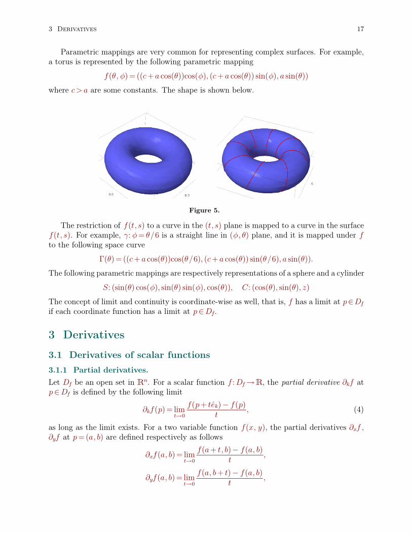
Parametric mappings are very common for representing complex surfaces. For example,a torus is represented by the following parametric mapping
f(�; �)= ((c+ a cos(�))cos(�); (c+ a cos(�)) sin(�); a sin(�))
where c> a are some constants. The shape is shown below.
Figure 5.
The restriction of f(t; s) to a curve in the (t; s) plane is mapped to a curve in the surfacef(t; s). For example, : �= �/6 is a straight line in (�; �) plane, and it is mapped under fto the following space curve
¡(�)= ((c+ a cos(�))cos(�/6); (c+ a cos(�)) sin(�/6); a sin(�)):
The following parametric mappings are respectively representations of a sphere and a cylinder
S: (sin(�) cos(�); sin(�) sin(�); cos(�)); C: (cos(�); sin(�); z)
The concept of limit and continuity is coordinate-wise as well, that is, f has a limit at p2Df
if each coordinate function has a limit at p2Df.
3 Derivatives
3.1 Derivatives of scalar functions
3.1.1 Partial derivatives.Let Df be an open set in Rn. For a scalar function f :Df!R, the partial derivative @kf atp2Df is defined by the following limit
@kf(p)= limt!0
f(p+ tek)¡ f(p)t
; (4)
as long as the limit exists. For a two variable function f(x; y), the partial derivatives @xf ;@yf at p=(a; b) are defined respectively as follows
@xf(a; b)= limt!0
f(a+ t; b)¡ f(a; b)t
;
@yf(a; b)= limt!0
f(a; b+ t)¡ f(a; b)t
;
3 Derivatives 17

as long as the limits exist.
Remark 1. For the sake of simplicity, we use the flat notations @x; @y in this book insteadof the standard ones @
@x;@
@y. Another notation for the partial derivative is fx; fy for
@f
@x;@f
@y.
Remark 2. Similarly, we can define partial derivative functions @xf ; @yf in the open setDf, the domain of f as
@xf(x; y)= limt!0
f(x+ t; y)¡ f(x; y)t
;
@yf(x; y)= limt!0
f(x; y+ t)¡ f(x; y)t
;
for (x; y)2Df.
Remark 3. The existence of partial derivatives of a function at a point does not guaranteesthe continuity of the function at that point. Consider the following function
f(x; y)=
(xy
x2+ y2(x; y)=/ (0; 0)
0 (x; y)= (0; 0):
Even though, @xf(0; 0); @yf(0; 0) exist and are equal zero, the function is not continuous atthe origin. However, f(x; y) must be continuous and differentiable with respect to x at (a; b)in order that @xf(a; b) exists. Similarly, f(x; y) must be continuous and differentiable withrespect to y at (a; b) in order that @yf(a; b) exists.
3.1.2 Interpretations of partial derivatives
Like a single variable function, there are two related interpretations of partial derivatives.Consider a two variable function f(x; y) defined on an open set Df. Fix a point (a; b) 2Df, and consider the horizontal line parallel to x-axis passing through (a; b). The partialderivative @xf(a; b) measures the rate of change of f at (a; b) along the horizontal line, andsimilarly, @yf(a; b) measures the rate of change of f at (a; b) along the vertical line passingthrough (a; b). For example, the rate of change of function f(x; y)= x2+ y2
pat (1;1) along
x-axis is
@xf(1; 1)=x
x2+ y2p ����������
(1;1)
=1
2p :
The slope of tangent lines to the surface of f(x; y) are expressed in terms of partial deriva-tives. The projection of line (a+ t; b), for t2 (¡c; c) for some c>0 on the graph of z= f(x; y)is a curve of the following form
¡1(t)= (a+ t; b; f(a+ t; b)):
This space curve passes through (a; b; f(a; b)) at t = 0. It is simply seen that @xf(a; b) isequal to the slope of tangent line to ¡1(t) in the (x; z)-plane at t=0:
d¡1dt
������t=0
=(1; 0; @xf(a; b))
18 Appendix

Similarly, @yf(a; b) is equal to the slope of tangent line to the curve ¡2(t) = (a; b + t;f(a; b + t)) at t = 0 in the (y; z)-plane. The following figure shows the graph of functionf(x; y)= x2+ y2
p, and the projection of 1(t)= (1+ t; 1) on it:
¡1(t)=¡1+ t; 1; 2+ t2+2t
p �:
The black line is the tangent to the space curve ¡1 at t=0. The slope of the tangent line, isthe tangent of the angle the line makes with the horizontal line 1, that is,
m=ddt
2+ t2+2tp
jt=0=1
2p :
Note that d¡1dt(0) is the tangent vector to the curve ¡1 at time 0
d¡1dt
(0)=
�1; 0;
1
2p�:
A similar argument holds for @yf , that is, if ¡2 is the projection of 2(t) = (1; 1 + t) on thegraph of f , then
d¡2dt
(0)=
�0; 1;
1
2p�:
Vectors d¡1dt(0);
d¡2dt(0) are both tangent to the graph of f at (1; 1; 2
p) and thus the plane
span�d¡1
dt(0);
d¡2dt(0)
is the tangent plane to the surface of f at (1; 1; 2p
). The algebraicequation of the tangent plane is derived by the air of n~
n~ = v~1� v~2=�¡ 1
2p ;¡ 1
2p ; 1
�;
3 Derivatives 19

and thus the algebraic of the tangent plane is derived as
¡ 1
2p (x¡ 1)¡ 1
2p (y¡ 1)+ z ¡ 2
p=0:
Remark 4. For a general function z= f(x; y), two principal tangent lines at p=(a; b) are
v~1=(1; 0; @xf(a; b)); v~2=(0; 1; @yf(a; b));
and thus n~ , the normal vector to the graph of f at p is
n~ =(¡@xf(p);¡@yf(p); 1):
Accordingly, the algebraic equation on the tangent plane at p is
¡@xf(a; b) (x¡ a)¡ @yf(a; b) (y¡ b)+ z¡ f(a; b)=0:
3.1.3 Chain ruleLet f be a scalar function on Df�R2, and assume that x; y are functions of another variable,say t, i.e., x = x(t); y = y(t). In the final analysis, f(x; y) is a function of t and thus theordinary derivative df
dtcan exist.
dfdt(t)= lim
h!0
f(x(t+h); y(t+h))¡ f(x(t); y(t))h
:
Proposition 7. Assume that f is differentiable with respect to x and y, and moreover thepartial derivatives are continuous. If x(t); y(t) are differentiable functions of t, then thefollowing equality that is called chain rule holds
dfdt
= @xf(x(t); y(t))dxdt
+ @yf(x(t); y(t))dydt: (5)
There is an important interpretation for the above formula. First, note that : (x(t); y(t))defines a parametric curve in the (x; y)-plane, and thus f(x(t); y(t)) can be considered as therestriction of f to . Also, we can consider as the path of a particle moving in the (x; y)-plane. Therefore, relation (5) states the rate of change of the value of that particle along .For example, if f is the density distribution function in the plane, then relation (5) stateshow fast or slow the density of a particle changes when it moves along path .
f( (0))
f( (t1)) (t)
f( (t2))
x
y
20 Appendix

On the other hand, since the graph of f is a surface in R3, f( (t)) is the projection of (t) in the surface as shown in the following figure. With this interpretation, relation (5)defines the slope of tangent to the curve at any instance of time.
Let us consider again equality (5) and rewrite it as follows
@xfdxdt
+ @yfdydt
=
�@xf@yf
��
0@ dx
dt
dy
dt
1A:Note that
0BB@ dx
dt
dy
dt
1CCA is just the tangent vector of the curve = (x(t); y(t)), i.e., 0(t). Vector @xf@yf
!is called the gradient of f and is denoted by grad(f) or rf . Therefore, equality (5)
can be rewritten asdfdt
=rf � 0(t);
and for this reason, df( (t))
dtis called also the derivative of f along (t). The chain rule can
be extended to higher dimensions. For example, if f(x; y) is a differentiable function withrespect to x; y and x=(x(t; s)); y= y(t; s) are differentiable functions then
@tf = @xf@tx+ @yf@ty;
@sf = @xf@sx+ @yf@sy:
Problem 50. If u=u(t; x), and x=x(t), find du
dt.
Problem 51. If u= f(x¡ 2t) find @tu and @xu.
3.1.4 Directional derivativePartial derivatives are just special cases of a more general derivative called the directionalderivative. Assume that a direction vector v = (v1; v2) is given (a direction vector is a unitvector), and f : Df ! R is a given continuous function. The directional derivative of f at(a; b)2Df along v is defined by the following limit
@vf(a; b)= limt!0
f(a+ tv1; b+ tv2)¡ f(a; b)t
;
3 Derivatives 21

as long as the limit exists. If so, then @vf(a; b) measures the rate of change of f at (a; b)along v. Obviously if v=(1; 0) then @vf(a; b)= @xf(a; b) and if v=(0; 1), it would be equalto @yf(a; b).
Proposition 8. If @xf ; @yf are continuous at (a; b), that is,
lim(x;y)!(a;b)
@xf(x; y)= @xf(a; b); lim(x;y)!(a;b)
@yf(x; y)= @yf(a; b);
then
@vf(a; b)=rf(a; b) � v
The continuity in the above proposition is crucial, for example, consider the followingfunction
f(x; y)=
8<: x2 y
x2+ y2(x; y)=/ (0; 0)
0 (x; y)= (0; 0):
If v=�
1
2p ;
1
2p�, then
@v(0; 0)= limt!0
t3
2 2p
t2
t=
1
2 2p ;
however, rf(0; 0) =�00
�, and thus rf(0; 0) � v = 0. The reason is that @xf ; @yf are not
continuous at (0; 0). To see this, let us find @yf for (x; y)=/ 0 as
@yf(x; y)=x2(x2¡ y2)(x2+ y2)2
;
and observe that @yf does not have even a limit at (0; 0). Note also that the directionalderivative of a function f is a special case of the chain rule rf � 0(t).
Problem 52. For the following function
f(x; y)=
8<: x2y
x4+ y2(x; y)=/ (0; 0)
0 (x; y)= (0; 0)
show that @rf(0; 0) exists for any direction r but partial derivatives are not continuous at (0; 0).
3.1.5 Gradient
Consider the level curve defined by : f(x; y)= c. If (t)= (x(t); y(t)) is a parametrizationof this curve then rf � 0(t)=0 for any t as long as rf is a continuous vector function. Thisrelation means that rf( (t)) is always perpendicular to (t). For example, the level curve
x4+2x2y+x2+ y2=1;
22 Appendix

has the gradient
rf =
4x3+4xy+2x
2x2+2y
!:
The following figure shows a few of gradient vectors �f on the level curve
As it is observed, gradient vectors are perpendicular to level curves. On the other hand, ifn=(n1; n2) is the direction vector at a point on the level curve, the the directional derivative@n~f of f is rf � n, and since n= rf
krf k (as long as the rf =/ 0), we obtain
@nf = krf k:
Therefore, the magnitude of �f at a point measures the rate of change of f along the normaldirection on the level curve. This result is extremely useful to maximize (or minimize) ascalar function. The procedure is as follows. To maximize f(x; y), we fix an initial pointp0=(x0; y0). The next point p1 is obtained by the following relation
p1= p0+�rf(p0)krf(p0)k
;
where �> 0 is a small value. Geometrically, that mean we take a step of length � along thedirection rf(p0). Iterating this procedure, that is,
pn+1= pn+�rf(pn)krf(pn)k
;
converges the maximum point of f as long such a local or global maximum exists, and if fsatisfies some other verifiable conditions.
In above, we used frequently the operator nabla r=
0BB@ @1���@n
1CCA. It is applied to differentiable
function as rf =0BB@ @1f
���@nf
1CCA. We study this operator in more detail later in this appendix.
3 Derivatives 23

Problem 53. Show the following relations
a) r(f + g)=rf +rg.
b) r(kf)= krf , k 2R.
c) r(fg)= frg+ grf .
3.1.6 Derivative and differential
Let f :Df �Rn!R be a scalar function defined on an open set Df. The derivative of f atp0 is the linear mapping Dp0f :R
n!R such that the following relation holds for any h~ 2Rn
limh~!0
f(p0+h~ )¡ f(p0)¡Dp0f(h~ )
kh~ k=0 (6)
Obviously if f is differentiable at p0 then it is continuous at that point. Moreover, sucha linear mapping must be unique. Note that if a function f is differentiable at a point athen directional derivatives along any direction at a exist. The reverse holds only if partialderivatives are continuous at a.
Problem 54. Verify that the above definition is compatible with the usual definition for single variablefunctions.
Problem 55. Show that if f is differentiable at p0 it must be continuous at that point. Show also thatits derivative (the linear mapping) is unique.
Proposition 9. Assume that f has continuous partial derivatives at p0, that is,
limp!p0
@kf(p)= @kf(p0);
for k=1; :::; n, then Dp0f exists and has the matrix representation
Dp0f = [@1f(p0); ���; @nf(p0)]:
According to the above proposition, if f has continuous partial derivatives at p0 then forany h~ 2Rn, the following relation holds.
Dp0f(h~ )=rf(p0) �h~ :
For this reason, some texts write Dp0f =rf(p0) that we should keep in mind that Dp0f isa 1�n matrix, while rf(p0) is a n� 1 vector.
24 Appendix

Example 6. For example, function
f(x; y)=
8<: x2y
x4+ y2(x; y)=/ (0; 0)
0 (x; y)= (0; 0)
has directional derivatives in all directions at the origin, however, the function is not dif-ferentiable at this point since it is not even continuous at the origin (why?). On the otherhand, functionf(x; y)=x2+ y2 has continuous partial derivatives @xf =2x; @yf =2y and forany p0=(x0; y0), we have
Dp0f =2[x0; y0]:
Let us verify definition (6) for f at p0=(1;¡1). For arbitrary h~ =(h1; h2), we have
limh~!0
(1+h1)2+(¡1+h2)2¡ 2¡ 2(h1¡h2)h12+h2
2p = lim
h~!0
h12+h2
2
h12+h2
2p = lim
h~!0kh~ k=0:
An immediate result of definition (6) is the linear approximation formula. If f :Df!Ris continuously differentiable at p02Df, that is
limp!p0
Dpf =Dp0f ;
then
f(p)� f(p0)+Dp0f(p~ ¡ p~0);
or equivalently
f(p)� f(p0)+rf(p0) � (p~ ¡ p~0):
For functions of two variables, the above formula reads
f(x; y)= f(x0; y0)+ @xf (x¡x0)+ @yf (y¡ y0):
Note that the right hand side is the equation of tangent plane at (x0; y0; f(x0; y0)):
T (x; y)= (x0; y0)+ @xf (x¡x0)+ @yf (y¡ y0):
Theorem 3. (Mean Value Theorem) Assume that f : Df ! R is continuously dif-ferentiable everywhere in Df. Fix a point p0 2 Df. Then for any point p 2 Df, there is� 2 tp+(1¡ t)p0, t2 (0; 1) such that
f(p)= f(p)+rf(�) � (p~ ¡ p~0):
Problem 56. Prove the theorem. Hint: define g(t)= f(tp+(1¡ t)p0) and apply the mean value theoremfor the single variable function g(t); t2 [0; 1].
3 Derivatives 25

Definition 12. The total differential of f :Df!R at p0 is defined by the following formula
df(p0)= @1f(p0) dx1+ ���+ @nf(p0) dxn:
Remember that for a single variable function y = y(t), the differential dy is defined bythe relation dy(t0)= y 0(t0) dt. Fig.(6) below shows this relation geometrically.
dt
dy(t0)
t0
y= y(t)
y(t0)
t0
dt
dy= y 0(t0) dt
y
t
T (x)
Figure 6.
Similarly for a 2-variable function z= f(x; y), dz is defined by the following relation andits geometry is represented in Fig. 7.
dz= @xfdx+ @yfdy:
(x0; y0)
dz= @xfdx+ @yfdy
dy
dx
x
y
f(x0; y0)
z
Figure 7.
3.1.7 Critical points and local max and min
Let Df �Rn be an open set. A point a2Df is called a local min (or max) of f :Df!R ifthere is a ball B�(a) such that f(p)� f(a) (alternatively f(p)� f(a)) for all p 2B�(a). Iff is differentiable at a, and if a is a local min or max, then Daf is a zero mapping. To see
26 Appendix

this, suppose a is a local min, choose an arbitrary direction vector h~ , and write
0= limt!0
f(a+ th~ )¡ f(a)¡Daf(th~ )
kth~ k= lim
t!0
f(a+ th~ )¡ f(a)¡ tDaf(h~ )jtj :
For t> 0, we have
Daf(h~ )= limt!0
f(a+ t h~ )¡ f(a)t
� 0
For t< 0, we have
Daf(h~ )= limt!0
f(a+ t h~ )¡ f(a)t
� 0;
and thus Daf(h~ ) = 0 for arbitrary h~ , and thus Daf is a zero mapping (meaning rf(a) is azero vector).
Definition 13. (Critical point) A point a is called a critical point of a function f if eitherDaf does not exist or Daf is a zero mapping. If Daf is a zero mapping, a can be a local min,local max, a saddle point or non of them.
In order to determine the type of a critical point in terms of min, max or saddle, weneed the notion of second derivatives. Second order partial derivatives @ijf are defined as@ijf = @i(@jf). We have the following theorem.
Theorem 4. Let Df�Rn be an open set, and f :Df!R . Furthermore assume that @ijf iscontinuous, then @ijf = @jif.
Theorem 5. Assume that f :Df!R is continuously differentiable of order 2 on open set Df.Fix a2Df, then there is � 2 tp+(1¡ t)a for some t2 (0; 1) such that the following relationholds for any for any p2Df
f(p)= f(a)+rf(a) � (p~ ¡ a~)+ (Hf(�)(p~ ¡ a~)) � (p~ ¡ a~);
where Hf is the Hessian matrix of f defined as Hf = [@ijf ]i;j.
Corollary 1. Assume that f is second order continuously differentiable function and rf(a)=0, then a is a local min if Hf(a) is a positive definite matrix, a is a local max if Hf(a)is a negative definite matrix, and a saddle point if Hf(a) has eigenvalues with opposite signs.
The standard example of above three cases is f = x2+ y2; f =¡x2¡ y2, and f = x2¡ y2
as shown below
3 Derivatives 27
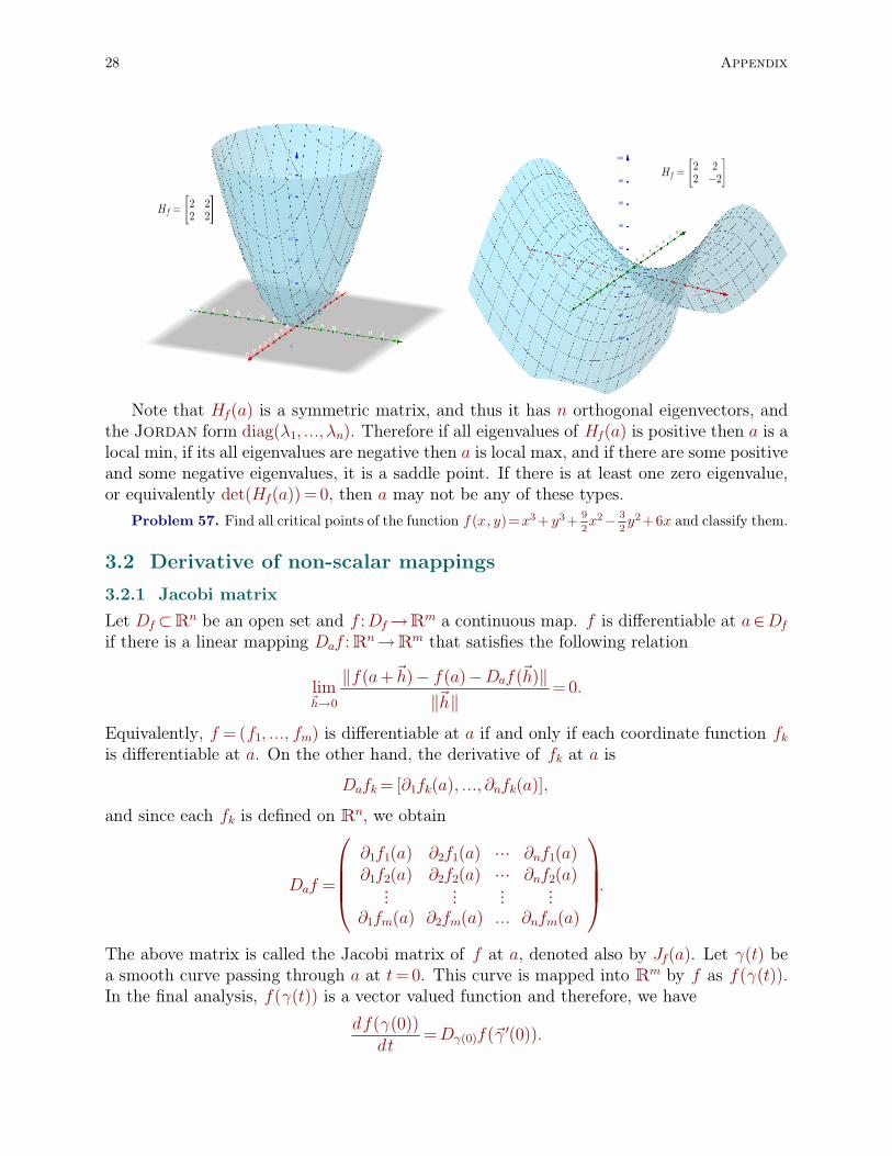
Note that Hf(a) is a symmetric matrix, and thus it has n orthogonal eigenvectors, andthe Jordan form diag(�1; :::; �n). Therefore if all eigenvalues of Hf(a) is positive then a is alocal min, if its all eigenvalues are negative then a is local max, and if there are some positiveand some negative eigenvalues, it is a saddle point. If there is at least one zero eigenvalue,or equivalently det(Hf(a))=0, then a may not be any of these types.
Problem 57. Find all critical points of the function f(x; y)=x3+ y3+ 9
2x2¡ 3
2y2+6x and classify them.
3.2 Derivative of non-scalar mappings
3.2.1 Jacobi matrixLet Df�Rn be an open set and f :Df!Rm a continuous map. f is differentiable at a2Df
if there is a linear mapping Daf :Rn!Rm that satisfies the following relation
limh~!0
kf(a+h~ )¡ f(a)¡Daf(h~ )kkh~ k
=0:
Equivalently, f =(f1; :::; fm) is differentiable at a if and only if each coordinate function fkis differentiable at a. On the other hand, the derivative of fk at a is
Dafk= [@1fk(a); :::; @nfk(a)];
and since each fk is defined on Rn, we obtain
Daf =
0BBBBBB@@1f1(a) @2f1(a) ��� @nf1(a)@1f2(a) @2f2(a) ��� @nf2(a)��� ��� ��� ���
@1fm(a) @2fm(a) ::: @nfm(a)
1CCCCCCA:The above matrix is called the Jacobi matrix of f at a, denoted also by Jf(a). Let (t) bea smooth curve passing through a at t=0. This curve is mapped into Rm by f as f( (t)).In the final analysis, f( (t)) is a vector valued function and therefore, we have
df( (0))dt
=D (0)f( ~ 0(0)):
28 Appendix

Since 0(0) is the tangent vector on (t) at t = 0, D (0)f( ~ 0(0)) is the tangent vector onf( (t)) at t=0. For example, for f(x; y)= (x2¡ y2; x2+ y2) we have
D(1;1)f =
�2 ¡22 2
�:
If (t) = (e¡t; et) (passing through (0; 0) at t= 0), we have 0(0) =�¡11
�and accordingly,
D (0)f( 0(0))=�¡40
�. Note that
ddtf( (t))jt=0=
ddt(e¡2t¡ e2t; e¡2t+ e¡2t)jt=0=
�¡40
�:
3 Derivatives 29
Theorem 6. Assume that the Jacobi matrix of a mapping f :Df �Rn!Rn is invertible ata. Then there is a neighborhood B�(a) such that f is one to one on B�(a).
Note that det(Jf(a)) measures the volume of a parallelogram constructed on columns ofJf(a). In other word, if C is a unit cube made at a, then det(Jf(a)) is equal to the volumeof parallelogram Jf(a)(C). Hence, if det(Jf(a))=/ 0, there is a neighborhood B�(a) such thatf is one to one on B�(a).
3.2.2 Smooth surfaces
Remember that a smooth space curve is represented by a curve map (t) such that 0(t) isnonzero. Geometrically, this condition means that (t) always admits a tangent vector thatvaries continuously along .
Definition 14. A surface S in R3 is called smooth if S has a nonzero normal (perpendicular)vector at all points on S.
Let f(t; s) 2 R3 be parametric surface. Consider an arbitrary point f(t0; s0) on S.Coordinate line 1(t)= (t+ t0; s0) is mapped on S as ¡1(t)= f(t+ t0; s0). The tangent vectorto this space curve is just ¡10(t0)=@tf(t0; s0). Similarly, the coordinate line 2(s)=(t0; s+s0)is mapped as ¡2(s)= f(t0; s+s0) and the tangent vector is ¡20(s)=@sf(t0; s0). Notice that both¡10;¡2
0 are tangent to S and therefore n~ :=¡10�¡20 is perpendicular to S as long as it is nonzero
n~ =
��������������i j k
@tx (t0; s0) @ty(t0; s0) @tz(t0; s0)@sx (t0; s0) @sy(t0; s0) @sz(t0; s0)
��������������=/ 0:Let us see the result for a smooth function z= f(x; y). The graph of function is
�(x; y)= (x; y; f(x; y));
and thus @x�=(1; 0; @xf) and @y�=(0; 1; @yf). The normal vector n~ is
n~ = @x�� @y�=(¡@xf ;¡@yf ; 1):
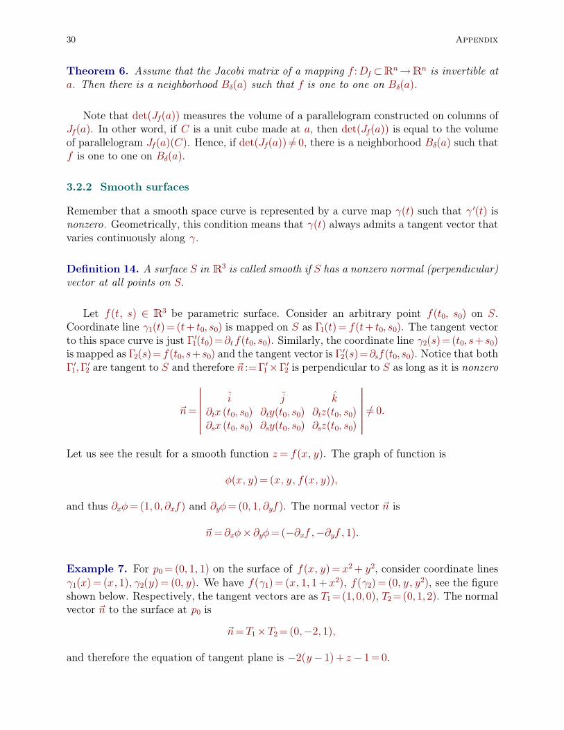
Example 7. For p0= (0; 1; 1) on the surface of f(x; y)= x2+ y2, consider coordinate lines 1(x) = (x; 1); 2(y) = (0; y). We have f( 1)= (x; 1; 1+ x2), f( 2)= (0; y; y2), see the figureshown below. Respectively, the tangent vectors are as T1=(1;0;0), T2=(0;1;2). The normalvector n~ to the surface at p0 is
n~ =T1�T2=(0;¡2; 1);
and therefore the equation of tangent plane is ¡2(y¡ 1)+ z ¡ 1=0.
30 Appendix

For a surface represented by the implicit function S: f(x; y; z) = 0, the normal vector n~is derived by the following procedure. Consider an arbitrary space curve =(x(t); y(t); z(t))on S, that is, f(x(t); y(t); z(t))=0. The chain rule states
dfdt( )=rf( (t)) � 0(t)=0:
Since 0(t) is tangent to S, then rf is perpendicular to (t) if rf is nonzero. On theother hand, since is arbitrary, then 0 belongs to the tangent plane on S, and thus rf isperpendicular to S. Therefore, we obtain n~ as
n~ =(@xf ; @yf ; @zf):
Problem 58. Write the equation of curve formed by the intersection of the unit sphere x2+ y2+ z2=4and the plane x+ y+ z=1.
3.3 Implicit function theoremAn implicit function f(x; y) = 0 defines generally a planar curve in the (x; y) plane. Ify= y(x), then by the chain rule, we can write
dydx
=¡@xf@yf
:
However, there is no guarantee in general that y could be solved in terms of x or x couldbe solved in terms of y. Question is this: is there any function y= g(x) defined on an openinterval I such that f(x; g(x))=0 for all x2 I. The following theorem answers the question.
Theorem 7. (implicit function theorem) Suppose implicit function f(x; y)=0 satisfiesthe following conditions
i. there is a point p0=(x0; y0) such that f(x0; y0)=0,
ii. there is an open ball B"(p0) such that f has continuous partial derivatives on it,
3 Derivatives 31

iii. and that @yf(x0; y0)=/ 0,
then there is an open interval I=(x0¡�;x0+�), and a function y= g(x) such that y0= g(x0),and f(x; g(x))=0 for all x2 I.
Example 8. Consider the following function
exy+ x+ sin(y)= 1:
The function defines a planar curve which is shown below in Fig.8.
-2 0 2-4
-2
0
2
4
x= − 0. 49
x=1. 96
Figure 8.
The slopes at x=¡0.49 and x= 1.96 are infinity, which implies @yf =0 at those pointsaccording to the formula y 0=¡@xf
@yf. Now fix the point p0=(0; 0) on the curve. As it is seen
from the figure, there is an explicit function y= g(x) for x2 (¡0.49; 1.96) such that
exg(x)+x+ sin(g(x))=1: (7)
The result can be generalized for functions f :Rn!R as follows.
Theorem 8. Assume that implicit function f(x1; x2; :::; xn) = 0 satisfies the followingconditions
i. there is a point a=(a1; a2; :::; an) such that f(a1; ���; an)= 0,
ii. There is an open ball B"(a) such that f has continuous partial derivatives on it,
iii. and that @nf(a)=/ 0,
then there exists a ball B� at a0 = (a1; ���; an¡1) and a function g: B�(a0) ! R such thatan= g(a1; ���; an¡1) and f(x1; x2; :::; g(x1; :::; xn¡1))=0 for all (x1; :::; xn¡1)2B�(a0).
32 Appendix

4 Integrals of mutivariable functions
4.1 Line integralsLet : (a; b)!Rn be a smooth curve map, that is 0(t)=/ 0. The length of (a; b) is definedby the following integral
L=
Za
b
j 0(t)j dt:
This definition coincides the intuitive notion of the length. For example, if the image of (t) is a curved metal wire, and if we straightened the wired, we get the same length if wecalculate the length by the above integration. In the above definition, 0(t) is the tangentvector on at t. The quantity dl= j 0(t)j dt is called the differential arc length.
Now let D�Rn be an open set and let be a smooth curve in D. Assume that f :D!Ris a continuous function. The integral of f along is defined by the following integral
I =
Za
b
f( (t))dl=
Za
b
f( (t)) j 0(t)j dt:
Geometrically this integral is equal to the surface area constructed on the base (t) an theheight f( (t)). In particular if f =1, the above integral gives the arc length of . If f denotethe density function of a metal wire represented by , the integral denote the total mass ofthe wire.
4 Integrals of mutivariable functions 33

Problem 59. Consider the metal wire in the shape of the semi-circle x2+ y2=1, y� 0. If the densityof the wire is given by �= k(1¡ y) for a constant k, find the center of mass of the wire.
4.2 Integrals over a bounded domain of R2
Now, let R: [a; b]� [c; d] be a rectangle and f :R�R2!R be a continuous function. Similarto the integrals of single variable function, we can define the following double integral
I =
Z ZR
f(x; y )dA;
by the aid of an infinite sum called the Riemann sum as
I = limn;m!1
Xj=1
m Xi=1
n
f(xi; yj) j�ij j:
Here �ij is a partition of R, j�ij j is the area of the rectangle ij and (xi; yj) is an arbitrarypoint in �ij. We have the following theorem. Geometrically, I denote the volume constructedon the base R, and height f .
Theorem 9. (Fubini) Assume that the f is continuous (or piecewise continuous) in R=[a;b]� [c; d]. Then we haveZ
R
f(x; y) dA=
Za
b�Z
c
d
f(x; y) dy
�dx=
Zc
d�Z
a
b
f(x; y) dx
�dy:
Now, assume that D � R2 is a closed bounded domain and assume that f : D! R iscontinuous. We can inscribe D inside a rectangle R and extend f on R as follows
f~(x; y)=
�f(x; y) (x; y)2D0 (x; y)2D :
Even though f~ may be discontinuous, we have the following factZ ZD
f(x; y) dA=
Z ZR
f~(x; y) dA:
Problem 60. Let I = [a; b] and assume that f(s; x) and @f
@x(s; x) are continuous in I � I. Use the
fundamental theorem of calculus and prove the following formula
ddx
Zx0
x
f(s; x) ds= f(x; x)+Zx0
x @@xf(s; x) ds:
In the proof you may need to pass the limit inside the integral.
4.3 Change of variables in multiple integralsOf most important techniques to calculate a double integral (and also triple integrals) is thechange of variable technique. Let D�R2 be a bounded domain, and assume f :D!R is acontinuous function. The goal is to calculate the integral
I =
Z ZD
f(x; y) dA:
34 Appendix

Now assume that there is a one to one mapping ': R �R2!D, where R is rectangle [a;b]� [c; d]. If so, then we can calculate I in terms of an integral over R. The advantage is thatthe integration over rectangular domains are much more simpler than general domains. Theprocedure is as follows. Let '(u; v)= (x; y), where (u; v)2R. See the following figure. Thedifferential area dA in (x; y)-plane in terms of the differential area dS in the (u; v)-plane is
dA= jdet(J')j dS;
where J' is the Jacobi matrix of the one to one transformation '.
u
v y
x
R
D'
dS
dA
Accordingly, we have the following formula called the change of variable techniqueZ ZD
f(x; y) dA=
Z ZR
f('(u; v)) jJ'(u; v)j du dv:
Problem 61. Find the domain D formed by the transforming rectangle [1; 2] � [1; 2] under thetransformation �
x=u/vy=uv
:
Calculate the following integral Z ZD
e y/xp
e xyp
dA:
4.4 Surface integrals over a surface in R3
Let S be a smooth surface in R3 with the representation
'(u; v)= (x(u; v); y(u; v); z(u; v));
where (u; v)2D�R2, and assume that f is a continuous functions defined on S: f :S!R.We want to calculate the following integral
I =
Z ZS
f(x; y; z) dA;
where dA is the differential area of the surface S. Here we again transform the integral overS as an integral over D as follows. Note that
dA= jj@u'� @v'jj dS;
4 Integrals of mutivariable functions 35

where dS is a differential area in D. Remember that @u' and @v' are tangent vectors onS and k@u '� @v 'k is equal to the area of parallelogram constructed on vectors @u'; @v'.Therefore, we can writeZ Z
S
f(x; y; z)dA=
Z ZD
f('(u; v)) jj@u'� @v'jjdS:
Problem 62. If f = f(x; y) is a smooth function defined on the bounded set D �R2, show that thearea of the surface associated to u is
A=ZD
1+ j@xf j2+ j@yf j2q
dx dy:
Problem 63. We show that the change of variable formula is independent of the transformation.
a) Assume ':D! S and :D1! S are two one to one transformations with image S. Define themap '~ := '¡1 � :D1!D. Verify
jj@t � @s jj= jj@u'� @v'jj jj@t'~� @s'~ jj:
b) Now show ZD
f('(u; v)) jj@u'�@v'jjdu dv=ZD1
f( (s; t))j@t � @s j dsdt:
We frequently use the polar and spherical coordinates for integrals. In polar coordinate,the transformation is defined by the relations '(r; �)= (r cos�; r sin�). The area differentialdS in this case is
dS=
�������� cos� sin�¡r sin� r cos�
�������� drd�= rdrd�:
If f(x; y) is a function defined in disk Ba, a disk of radius a centered at the origin, its doubleintegral in the polar coordinate isZ
Ba
f(x; y)dA=
Z0
2�Z0
a
f(r cos�; r sin�) rdrd�:
Problem 64. Show the following inequality
�4(1¡ e¡a2)�
Z0
aZ0
a
e¡x2¡y2ddxdy � �
4(1¡ e¡2a2);
and conclude
lima!1
Z0
aZ0
a
e¡x2¡y2dA= �
4:
Use the above result and find
I =Z0
1e¡x
2dx:
In the spherical coordinate, the transformation is
'(�; �; �)= (� cos� sin�; � sin� sin�; � cos�):
The volume differential in this coordinate is
dV =
������������sin� cos� sin� sin� cos�� cos� cos� � cos� sin� ¡� sin�¡� sin� sin� � sin� cos� 0
������������ d�d�d�= �2sin�d�d�d�:
36 Appendix

If f(x; y; z) is defined, for example, in a sphere of radius a, its integral on this sphere is equalto Z
Sa
f(x; y; z)dS= a2Z0
2�Z0
�
f(a sin� cos�; a sin� sin�; a cos�) sin�d�d�:
5 Calculus of vector fields
5.1 Vector fieldLet D�Rn be an open set. A vector field is a mapping f :D!Rn. For each p2D, f(p) isa vector in Rn, and thus we can interpret this mapping as an assignment a vector f(p) toevery point p2D, that is, p 7! f(p). This assignment is called a vector field .
A vector field p 7! f(p) is continuous if the association varies continuously with respect top, that is, the any change from p to an adjacent point q, the vector f(p) continuously variesto f(q). Mathematically speaking, this is equivalent to the continuity of f as a mappingon D. Remember that f = (f1; :::; fn) is a continuous mapping if and only if each scalarfunction fk is a continuous function. Similarly, a vector field p 7! f(p) is called continuouslydifferentiable if and only if all its coordinate functions are continuously differentiable.
A vector fields models many physical phenomena. For example, an electrical charge qlocated at the origin, generates an electrical field in the space as
E(r)=q
4�"0
r~kr~ k3 ;
where "0 is the permittivity constant of the space. This field is a force field an is completelysimilar to the gravitational field generated by a mass M :
g(r)=GMr~kr~ k3 ;
where G is the universal constant.
5.2 Vector fields and differential equationsThe theory of ordinary differential equations can be formulated in terms of vector fields. Infact, the system 8>>>><>>>>:
dx1dt= f1(x1; :::; xn)
���dxndt= fn(x1; :::; xn)
:
defines a vector field f = (f1; :::; fn) on some domain D, and a parametric curve (t) =(x1(t); :::; xn(t)) such that the tangent vector on at each instant of time t0 that is 0(t0)coincides with the vector assigned to point (t0). In other word, f( (t)) = 0(t) for all t inan open interval. For example, the following system�
x0=¡yy 0=x
;
5 Calculus of vector fields 37

defines vector field f =(¡y; x). As we know, the trajectory of a point p0: (x0; y0) accordingto the above system is the line
(t)= (x0 cost¡ y0 sint; x0 sint+ y0 cost):
It is simply seen that
0(t)= (¡x0 sint¡ y0 cost; x0 cost¡ y0 sint);
that is equal to f( (t)). Notice that (t) is just the rotation mapping applied to po
(t)=
�cost ¡sintsint cost
��x0y0
�;
that coincides with the geometry of vector field f3.
5.3 Gradient fieldA vector fiend p 7! f(p) is called a potential, conservative or just gradient field if there isa scalar function � such that f = ¡r�. The negative sign is just for historic reason. Forexample, the electric field E(r) or the gravitational field g(r) are potential. It is simply seenthat E(r)=¡r�, where � is the following scalar function:
�(r)=q
4�"0
1kr~ k :
Potential fields satisfies very nice properties that we study in sequel. In the following figure,three vector fields are shown: f1=(x; y), f2=(¡x;¡y), and f3=(¡y; x).
−1. 0 −0. 5 0. 0 0. 5 1. 0−1. 0
−0. 5
0. 0
0. 5
1. 0
−1. 0 −0. 5 0. 0 0. 5 1. 0−1. 0
−0. 5
0. 0
0. 5
1. 0
−1. 0 −0. 5 0. 0 0. 5 1. 0−1. 0
−0. 5
0. 0
0. 5
1. 0
It is seen that f1; f2 are potential field with potentials �1=¡1
2x2¡ 1
2y2, �2=
1
2x2
1
2y2. The
filed f3 is not potential, i.e., there is no potential function � such that f3=r�.Problem 65. Prove the above claim, that is, show there is no scalar function � such that f3=r�.
The force field generated by a potential is also called conservative. To see the reason, letus write the second Newton's law for a unit mass as8<:
d2x
dt2= p(x; y)
d2 y
dt2= q(x; y)
;
38 Appendix

where the field f =(p; q) is potential generated by a potential function �(x; y). Let (t) bethe trajectory of a particle initially located at (x0; y0). Then we have
00(t)= f( (t))=¡r�( (t)):
Let us define the energy along (t) as follows
E(t)=12k 0(t)k2+ �( (t)):
The derivative of E along (t) is then
dEdt
= 00(t) � 0(t)+ ddt�( (t)):
We haveddt�( (t))=r�( (t)) � 0(t);
and thusdEdt
= 00(t) � 0(t)+r� � 0(t)= ( 00+r�) � 0=0:
Therefore, the derivative of the energy function along a trajectory (t) is zero, in other world,the energy is conserved along the trajectory of the particle.
5.4 Divergence, curl and LaplacianTwo important operations on smooth vector fields are divergence and curl. The divergenceof a field f =(f1; :::; fn) at a point p is defined by the following relation
div f(p)=@1f1(p)+ ���+ @nfn(p)
It is simply seen that the divergence of a vector field f is equal to the dot product ofnabla r and field f as div f =r:f . It is also equal to the trace of matrix Dpf . Intuitivelyspeaking, div f(p) measure the flow of net flux passing through p. If div f(p)> 0, point pacts like a source that emits or generate flow. All points in filed f1=(x; y) are source pointssince div f(p) = 2. If div f(p)< 0, point p acts like a sink that absorbs or attracts flow toitself. All points in field f2=(¡x;¡y) are sink since div f(p)=¡2. If div f(p)=0, then thenet flow passing through p is zero, that the net amount of incoming flow is equal to outgoingflow. All points in field f3=(¡y; x) are of this type.
Problem 66. If � is a smooth scalar function and let f be a smooth vector field, show the followingformula
div (�f)= �div f + f �r� (8)
Another important operation regarding a vector field in R3 is the curl of the field at apoint. The curl of a vector field f =(f1; f2; f3) at p is defined by the following relation
cur(f)(p)=
0BB@ i j k@x @y @zf1 f2 f3
1CCA(p)= (@2f3¡ @3f2; @3f1¡ @1f3; @1f2¡ @2f1)(p):
5 Calculus of vector fields 39

Symbolically, we can write the curl in terms of r as r� f . Since curl(f) is a vector at everypoint, it also defines a new vector field in its domain. At each point p, curl(f)(p)measures therotation of vector field f in three directions: 1) component @2f3(p)¡ @3f2(p) that measuresthe rotation of f at p around x-axis, 2) component @3f1(p) ¡ @1f3(p) that measures therotation of f at p around y-axis, 3) and @1f2(p)¡@2f1(p) that measure the rotation aroundz-axis . For example, curl (¡y; x)= 2 k at all points, that means the filed rotates around z-axis with constant speed at all points. This rotation is evident from the figure of the field.
Assume that � is a smooth scalar function defined on an open subset D of Rn. TheLaplacian of � is defined by the following relation
��= @11�+ ���++@nn�:
It is simply seen that ��=div (grad �).
Problem 67. Consider field f =(x2¡ y2; y2¡ z2; z2¡x2).
a) Find r� f at the point (1; 2; 3).
b) Verify that (r� f): i is equal to r� (0; y2¡ z2; z2¡ 1).
Problem 68. Assume that � is a smooth scalar function defined in R3. Show r�r�=0.
Problem 69. Show the following relations for smooth fields f ; g in R3 and smooth function �
a) r� (�f)= �r� f ¡ f � (r�).
b) r:(f � g)= g:(r� f)¡ f(r� g).
Problem 70. If f is a smooth vector field, what is r: (r� f)?
Problem 71. Show the following relation
r� (r� f)=r(r:f)¡�f ;
where �f =(�f1;�f2;�f3) for a smooth vector field f =(f1; f2; f3).
5.5 Line integrals in vector fieldsAssume that the f :D�Rn!Rn is a continuous field, and C is a smooth curve in D. Wedefine a method for the integral of f along curve C. For this, we take a parametrization ofC as : (a; b)!D, where (a; b)=C. The desired integral is defined as followsZ
C
fdc=
Za
b
f( (t)) � 0(t) dt: (9)
It is seen that the integral is independent of parametrization, that is, if 1: (c; d)! D isanother parametrization of C, then
I =
Zc
d
f( 1(t)) � 10(t) dt:
Problem 72. Assume that : (a; b)!D, 1: (c; d)!D are two smooth parametrizations of C. Showthe relation Z
a
b
f( (t)) � 0(t)dt=Zc
d
f( 1(t)) � 10(t) dt:
40 Appendix

If f is a force field, then the integral of f along a curve is called the work done by f . Forexample, let (a)= p0, (b)= p1, then I measure the total work done by f to move a particlefrom point p0 to point p1 along path . It is is interesting to note that if f is gradient, i.e.,f =r� for some potential �, then the integral is independent of path along a particle movesfrom p0 to p1. This important fact is shown belowZ
a
b
r�( (t)) � 0(t) dt=Za
b
d�( (t))= �( (b))¡ �( (a))= �(p1)¡ �(p0):
The path independence property of a field implies that the integral of field over any closedcurve is zero, that is, if is a closed curve thenI
f( (t)) � 0(t) dt=0: (10)
We have the following theorem.
Theorem 10. Assume f :D�Rn!Rn is a smooth vector field. If the integral of f over allclosed curves in D is zero, then f is a conservative field on D.
Problem 73. Let the condition of the above theorem holds. Fix p02D. For any p2D define � as
�(p)=Z0
t
f( (t)) � 0(t) dt;
where (t) is an arbitrary smooth curve in D such that (0)= p0, and (t)= p.
a) Verify that � is independent of path
b) Show that � is a potential for f . For example, for two dimensional field f = (p(x; y); q(x; y)),verify the relation
limh!0
�(x+h; y)¡ �(x; y)h
= p(x; y); limh!0
�(x; y+h)¡ �(x; y)h
= q(x; y):
Problem 74. A smooth field f =(p; q) in R2 is called exact if for all (x; y)2R2 the following relationholds
@yf(x; y)= @xq(x; y):
a) Show that f is conservative.
b) Consider field f=�
¡yx2+ y2
;x
x2+ y2
�defined everywhere inR2 except the origin. Show the following
relation
@y
�¡y
x2+ y2
�=@x
�x
x2+ y2
�:
Now, consider closed curve (t)= (cos t; sin t), t2 [0; 2�], calculate the line integral of f along .The result is nonzero. Does it contradict the fact claimed in (a)?
5.6 Surface integrals in vector fieldsLet S be a surface in R3 parameterized by a smooth map ¡(t; s) where (t; s)2D for someopen domain D. Note that ¡ is smooth if @t¡�@s¡ is nonzero for all points in D. Let smoothfield f =(f1; f2; f3) given in R3. The integral of f on the surface S is defined by the followingintegral
I =
ZZS
f � n dA ;
5 Calculus of vector fields 41

where n is the unit normal vector on S. This integral measures the total flux passing outwardthrough surface S. As it is shown in the following figure, the tangential component of fnever leaves the surface (due to the fact f � n = 0), and only the normal component of fcontributes in the total flux. For example, the flow of water through a window measured inm3
sec is a physical model for the flux.
n
f
dsnormal component
of f
tangent componentof f
Remark 5. In some branches of mathematics, the term flux is considered as a vector andnot scalar. We will see this notion in the book for the mathematical modeling of heat flowthrough a conductive media.
For the parametrization ¡(t; s), we have
n dA=(@t¡� @s¡) dt ds;
and therefore, the total flux is expressed in terms of double integral
I =
ZZD
f(¡(t; s)) � (@t¡� @s¡) dt ds:
Theorem 11. (divergence) Assume D � R3 is an open set with smooth (piecewise)boundary. If f is a smooth vector field in cl(D), the following relation holdsZZZ
D
div f dv=ZZ
bnd(D)f � n dA: (11)
Note that If div f = 0 inside D, then the net amount of flow passing through bnd(D)is zero. Accordingly, the divergence of a field f in R3 at a point p can be defined by thefollowing formula
div (f)(p)= limr!0
1Vol(Br(p))
ZZ
bnd(Br(p))f � n dA: (12)
The above formula coincides with our previous statement about the physical interpretationof divergence operator at a point, that div (f)(p) measures the net flux of f passing throughpoint p.
Problem 75. Let f =(x; y; z). Verify the formula (12) at the origin.
Example 9. Consider the identity field f(x; y; z) = (x; y; z), and let B be the closed unitball in R3 centered at the origin. The left hand side of formula (11) readsZZZ
B
div fdV =3
ZZZB
dV =4�: (13)
42 Appendix

The unit normal to bnd(B) is n=(x; y; z), and then the right hand side of formula (11) readsZZ
bnd(B)(x2+ y2+ z2) dA=
ZZ
bnd(B)dA=4�: (14)
Problem 76. Assume f :D�R3!R3 a smooth field. Use the divergence theorem and showZZZD
�f dV =ZZ
bnd(D)@nf ds; (15)
where @nf is the directional derivative of f in direction n.
Problem 77. If D is a ball of radius R in Rn, use the divergence theorem and show
Vol(D)= RnA(D);
where Vol(D) is the volume of D and A(D) is the surface area of D. (Hint: consider the function�=
Pkxk
2).
Problem 78. Let f be a smooth field in Rn such that
jf(r)j � 1(1+ jjr jj)n+1 :
Show that ZRn
div (f)=0:
Proposition 10. (Integration by parts) Let D�R3 be an open set and f ; g:D!R aresmooth functions. We haveZZZ
D
(@xf) g dV =
ZZ
bnd(D)fgn1 dA¡
ZD
f (@xg) dV ; (16)
where n1 is the first component of n=(n1; n2; n3i at bnd(D). Similar relations hold for thederivatives with respect to other components y; z.
The following proposition generalizes the above result.
Proposition 11. Let D be a domain in R3 and bnd(D) is smooth. If f is a smooth vectorfield in D and g is a smooth function on D thenZZZ
D
g div (f) dV =
ZZ
bnd(D)g (f � n) dA¡
ZZZD
f �rg dV : (17)
Problem 79. Prove the above proposition by the aid of divergence theorem.
Problem 80. By the above proposition showZZZD
g�fdV =ZZ
bnd(D)g @n fdA¡
ZZZD
rf �rg dV ;
and conclude the following relation called the Green's formula:ZZZD
(g�f ¡ f�g) dV =ZZ
bnd(D)[g @nf ¡ f@n g] dA:
5 Calculus of vector fields 43

Let S be a smooth surface in R3 with smooth boundary bnd(S). If f is a smooth fieldin R3, the following relation is called the Stoke's theorem:ZZ
S
(r� f) � n dA=Ibnd(S)
f � T dl;
where T is the unit tangent vector on curve bnd(S) and d` is the differential length of thatcurve.
Problem 81. Use the Stoke's theorem and show
(r� f(p)) � i = limr!0
1�r
Z0
2�
f( (t)) � 0(t) dt;
where (t) = p + (r cost; r sint; 0). Derive similar formula for the second and third components, i.e.,(r� f(p)) � j , and (r� f(p)) � k. Notice that f � T measures the rotation of f along curve bnd(S).
Problem 82. Let f=(¡y+x;¡x+z;¡z+ y). Verify the relations of the previous problem at the origin.
Problem 83. Show the following relations
a) ZZS
� curl(f) � n dA=ZZ
S
(f �r�) � n dA+Ibnd(S)
�f � T dl:
b) ZZZD
� div (f) dV =ZZ S
�f � n dA¡ZZZ
D
f �r�dVc) ZZZ
D
g � curl(f) dV =ZZ S
(f � g) � n dA+ZZZ
D
f � curl(g) dV
We have the following theorem
Theorem 12. If r� f =0 everywhere, then f is gradient, i.e., there is a potential function� such that f = ¡r�. If div (f) = 0 everywhere, then there is a vector field g such thatf = curl(g).
6 Orthogonal curvilinear coordinatesIn many applications, it is convenient to use an orthogonal coordinate rather than the Carte-sian one. The form of differential operators in a general orthogonal curvilinear coordinate isdiscussed below.
6.1 Unit vectorsLet (q1; q2; q3) be a curvilinear coordinate system, and assume (q1; q2; q3)!!!!!!!!
T(x; y; z) is a one
to one transformation to the Cartesian space. We first define the unit vectors q1; q2 and q3in the directions of q1; q2 and q3, and by the aid of that define the orthogonality notion. Ifwe consider the restriction of T to q1 as a one parameter map (q1), then the unit vector q1can defined as
q1: = 0(q1)k 0(q1)k
=@q1Tk@q1T k
;
44 Appendix

and sinceT (q1; q2; q3)= (x(q1; q2; q3); y(q1; q2; q3); z(q1; q2; q3));
we have@q1T =(@q1x; @q1y; @q1z)
Similarly, we can define q2; q3 as
q2=@q2Tk@q2T k
; q3=@q3Tk@q3T k
:
A coordinate system (q1; q2; q3) is called orthogonal if q1; q2 and q3 are mutually orthogonal,i.e., h qi; qji= �ij.
6.1.1 Polar, cylindrical and spherical coordinatesThe polar coordinate (r; �) is defined by the transformation T (r; �) = (r cos�; r sin�) forr=[0;1) and �2 [0;2�). The transformation is one to one everywhere in the domain exceptat the origin. Since @rT = cos� i + sin � j , we obtain
r= cos� i + sin � j :
Similarly, @�T =¡r sin � i + r cos � j , and thus
�=¡sin � i + cos � j :
� r
The cylindrical transformation is defined by transformation
T (r; �; z)= (r cos�:r sin�; z)The unit vectors are derived as
r= cos � i + sin � j ; �=¡sin � i + cos � j ; z= k:
The spherical coordinate is defined by the transformations
T (�; �; �)= (� cos� sin�; � sin� sin�; � cos�);
for �2 [0;1); �2 [0;2�); �=[0; �]. The mapping is not one to one at �=0; �=0; �. The unitvectors are
�= sin� cos� i + sin� sin� j + cos� k; (18)
�=¡sin� i + cos� j ; (19)
�= cos� cos� i + cos � sin� j ¡ sin � k: (20)
6 Orthogonal curvilinear coordinates 45

6.2 Nabla r in an orthogonal coordinateLet f be a smooth scalar function given in an orthogonal coordinate system (q1; q2; q3). Wecan write the gradient of f in this system as
rf = f1 q1+ f2 q2+ f3 q3;
that implies f1= hrf ; q1i, f2= hrf ; q2i, and f3= hrf ; q3i. Let us calculate f1 for example.rf is coordinate free, and thus we can replace its form in the Cartesian coordinate, i.e.,rf = @xf i + @yf j + @zf k in the associated dot product and derive
hrf ; q1i=1
k@q1T kh@xf i + @yf j + @zf k; @q1x i + @q1y j + @q1z ki:
By the orthogonality, we obtain
hrf ; q1i=1
k@q1T k(@xf@q1x+ @yf@q1y+ @zf@q1z)=
1k@q1T k
@q1f:
We obtain similar forms for f2; f3, that are,
hrf ; q2i=1
k@q2T k@q2f ; hrf ; q3i=
1k@q3T k
@q3f
and therefore the operator r in (q1; q2; q3) is
r=q1
k@q1T k@q1+
q2k@q2T k
@q2+q3
k@q3T k@q3:
6.2.1 Polar, cylindrical and spherical coordinate
Applying the formula obtained above for polar, cylindrical and spherical systems gives respec-tively
Polar: r= r @r+1r� @�:
Cylindrical: r= r @r+1r� @�+ k @z:
Spherical: r= � @�+1
� sin �� @�+
1�� @�:
To calculate the Laplacian operator � :=r:r in (q1; q2; q3) system, we do as follows:
�:=r:r=
�q1
k@q1T k@q1+
q2k@q2T k
@q2+q3
k@q3T k@q3;
q1k@q1T k
@q1+q2
k@q2T k@q2+
q3k@q3T k
@q3
�:
Here we need @i( qj) for i; j=1; 2; 3. It turns out that the derivatives of qk always lies in thenormal plane to it, for example,
@q2( q1)=� q2+ � q3:
The reason is for the relation h qi; qii=1 and thus h@qj( qi); qii=0.
46 Appendix

Problem 84. In polar coordinate, show the following relations
@� r= � ; and @� �=¡r ; (21)
and conclude
�f = @rrf +1r@rf +
1r2@��f: (22)
Problem 85. In cylindrical coordinate show the relation
�f = @rrf +1r@rf +
1r2@��f + @zzf:
Problem 86. In spherical coordinate show the following relations
@� �= sin(�) � and @� �= � ; (23)
@� �=¡sin(�) �¡ cos(�) � and @� �=0; (24)
@� �= cos(�) � and @� �=¡�: (25)
and conclude
�f = 1�2@�(�2 @�f)+
1�2 sin2�
@��f +1
� 2sin �@�(sin�@�f):
7 Function Series
Working in a function vector space where functions play the role of well-known vectors inRn, requires to study sequences whose elements are functions. These type of sequences area natural generalization of numeric sequences that we suppose the reader is familiar with.
7.1 The different notions of convergenceWe assume that the reader is familiar with numeric sequences. Here we consider sequencesand series whose elements are functions. Let fn: [a; b]!R for n= 1; 2; ::: be a sequence ofcontinuous functions. We say fn converges pointwise in [a; b] to f , and write fn! f if
limn!1
jfn(x)¡ f(x)j=0;
for all a2 [a; b]. In other word, if an= fn(x) for a fixed x, then (an) as a numeric sequenceconverges to value b = f(x). This notion of convergence is equivalent to the following: forevery x2 [a; b] and every "> 0, there is an integer N0=N0(x; ")> 0 such that
8n�N0)jfn(x)¡ f(x)j<":
A function sequence fn converges uniformly to f in [a; b] if for for any " > 0, there is andinteger N =N(") such that
8n�N0) maxx2[a;b]
jfn(x)¡ f(x)j<":
The norm of a continuous function in a closed interval [a; b] is defined as
kf k= maxx2[a;b]
jf(x)j:
7 Function Series 47

For this reason, the uniform convergence is usually written as
limn!1
kfn¡ f k=0:
Remark 6. The pointwise and uniform convergence are two different types of convergenceand they may should not be considered as equivalent. In fact, if fn ! f uniformly, thenfn! f pointwise, while the converse is not generally true. For example, consider the sequenceof functions fn(x) = xn in [0; 1]. The sequence converges pointwise to f(x) =
�1 x=10 otherwise
.However, it is seen
maxx2[0;1]
jxn¡ f(x)j> 12;
and thus fn does not converges uniformly to f . In fact, fn does not converge uniformly toany function.
Problem 87. If a function sequence (fn) converges pointwise or uniformly, then its limit function isunique.
Problem 88. If a function sequence (fn) converges uniformly to f in [a; b] then it converges pointwiseto f as well.
Problem 89. Assume that fn: [a; b]!R is a sequence of continuous functions converges uniformly tof(x). Show that f(x) is continuous.
There are other notions of convergence that we study in the book, for example, theconvergence in norm as
limn!1
Za
b
jfn(x)¡ f(x)jdx=0:
For example, fn(x) = xn in [0; 1] converges to f(x) =�1 x=10 otherwise
or f(x) � 0 or f(x) =(1 x=
1
2
0 otherwise. As we see, the limit function is not unique in the usual sense, and we have to
do something to remedy this situation.
Problem 90. If (fn) converges uniformly to f in [a; b], it converges to f in the following senseZa
b
jfn(x)¡ f(x)jdx! 0:
Problem 91. Assume that a function sequence (fn) of continuous functions on [a; b] converges in normto f as Z
a
b
jfn(x)¡ f(x)jdx! 0Show that
limn!1
Za
b
fn(x) dx=Za
b
f(x) dx:
7.2 �-sequenceA function sequence fn(x) is called a Dirac �-sequence function at x=0 if for any continuousbounded function g(x) at x=0, we have
limn!1
Zg(x) fn(x) dx= g(0):
48 Appendix

For example, the sequence
fn(x)=
(n
2¡ 1
n<x<
1
n
0 otherwise;
is a �-sequence. If g(x) is any bounded continuous function at x=0, then
minx2�¡ 1
n;1
n
� g(x)�Z¡ 1
n
1
n
g(x)n2dx� max
x2�¡ 1
n;1
n
� g(x);and thus
limn!1
Z¡ 1
n
1
n
g(x)n2dx= g(0):
7.3 Differentiation and integration of function sequencesLet (fn) be a function sequence in (a; b) or [a; b]. If fn! f pointwise or uniformly, can weclaim Z
a
b
fn(x)dx!Za
b
f(x)dx
when n!1? Let us see an important example:
fn(x)=
8>>>><>>>>:22nx x2
�0;
1
2n
�2n(2¡ 2nx) x2
� 1
2n;
1
2n¡1
�0 otherwise
:
The graph for some n are shown in Fig.9. Each function fn is a triangle with the base�0;
1
2n¡1
�and the height 2n such that the area under each triangle is equal 1 independent of n.
4
2
11
2
8
1
4
1
8
Figure 9.
Therefore, we have for all n: Z0
1
fn(x)dx=1:
7 Function Series 49

On the other hand, it is seen fn converges to f � 0 on [0; 1] (why?) and thusZ0
1
fn(x)dx9Z0
1
f(x)dx:
In other word,
limn!1
Zfn(x) dx=/
Zlimn!1
fn(x)|||||||||||||||||||||||||||||||||||||||||||||||||| |{z}}}}}}}}}}}}}}}}}}}}}}}}}}}}}}}}}}}}}}}}}}}}}}}}}} }f(x)
dx:
Problem 92. Assume that (fn), fn: I!R is a sequence of continuous functions converging uniformlyto f . Show
limn!1
Za
b
fn(x) dx=Za
b
f(x) dx:
The following theorem gives a sufficient condition for passing the limit inside an integral.
Theorem 13. (dominant convergence) Assume that (fn) is a sequence of continuousfunctions converging pointwise to a function f in (a; b)(the interval may be finite or infinite).If there is a function g(x) such that
jfn(x)j � g(x); 8x2 (a; b);and Z
a
b
g(x) dx<1;
then
limn!1
Za
b
fn(x) dx=
Za
b
f(x) dx:
We also need the following form of the above theorem.
Corollary 2. Assume that f(t; x) is a continuous function defined on (c; d)� (a; b), andfurthermore
f(t; x)� g(x); 8t2 (c; d)such that Z
a
b
g(x) dx<1Then function
F (t)=
Za
b
f(t; x) dx;
is continuous in (c; d).
Problem 93. Prove the corollary by the aid of Theorem (13).
The same story of differentiation is the same. If a sequence of differentiable functions(fn) converges pointwise or even uniformly to f , then there is no guarantee that fn0! f 0. Asa simple example, sequence fn(x) =
1
nsin(nx) defined on (0; �) converges uniformly to the
constant function f(x)=0. However, fn0(x)= cos(nx) which is not a convergent sequence.
50 Appendix