Appendices for:

Developing dynamic, mechanistic species distribution models: predicting bird-mediated spread of invasive plants

across northeastern North America

Cory Merow, Nancy LaFleur, John A. Silander Jr., Adam M. Wilson and Margaret Rubega

Table of Contents

Appendix S1: Considerations for developing robust GB models..........................................................................2

Appendix S2: Sensitivity Analysis........................................................................................................................... 5Table S1. Summary of Sensitivity Analysis on Parameters.............................................................................................10Table S2. Summary of Sensitivity Analysis on Model Assumptions...............................................................................11Figure S1: No plant population growth.............................................................................................................................. 12Figure S2: No local bird dispersal...................................................................................................................................... 13Figure S3. No long distance dispersal............................................................................................................................... 13Figure S4. Homogeneous landscape................................................................................................................................. 14Figure S5. Homogeneous landscape with no LDD........................................................................................................... 15Figure S6: Binary Landscape............................................................................................................................................. 16Figure S7: Random Landscape.......................................................................................................................................... 17Figure S8: First Introductions in South............................................................................................................................. 18Figure S9: First Introductions in North.............................................................................................................................. 18Figure S10: First Introductions in Center.......................................................................................................................... 19Figure S11: First Introductions in West............................................................................................................................. 19Figure S12: First Introductions in East.............................................................................................................................. 20Figure S13: Long term predictions.................................................................................................................................... 20Figure S14: Random LDD Neighborhood 25 x 25............................................................................................................ 21Figure S15: Random LDD Neighborhood 51 x 51............................................................................................................. 21Figure S16: Start model in 1939......................................................................................................................................... 22Figure S17: Start model in 1959......................................................................................................................................... 22Figure S18: Shorter Bird Dispersal and More LDD........................................................................................................... 23

Appendix S3: Additional Data and Analysis......................................................................................................... 24Table S3. Growth Rate and Habitat Use Data.................................................................................................................... 24Table S4: LULC Reclassifications...................................................................................................................................... 25Figure S19. Seed dispersal kernel estimates.................................................................................................................... 26Figure S20. Christmas Bird Counts for Potential Bittersweet Dispersers......................................................................27Figure S21. Consequences of eradication efforts in CT and RI.......................................................................................27

Appendix S4: Model Code……………………………………….……………………………………………...……….………………..28

1

2

3

4

5

6

789

101112131415161718192021222324252627

2829303132333435

36

Appendix S1: Considerations for developing robust GB models

In order to appreciate the strengths and weaknesses in our models, it is necessary to understand the context

in which they were conceived and appropriate expectations about their predictions. Most importantly, GB models

provide the opportunity for mechanistic modeling, in contrast to statistical models that are typically phenomenological.

Our goal was to see how a few simple mechanisms interact, then determine how tradeoffs between model

parameters lead to categorically different types of predictive behavior. In contrast, detailed studies of species’

performance in different environments can generate detailed demographic predictions (e.g. Leicht 2005; Leicht-

Young 2007), but such models necessarily focus on small spatial scales and often fail to capture an understanding of

mechanistic linkages (e.g. dispersal and spread) or broad patterns. So what should an ecologist do when faced with

understanding broad scale dynamics based on some insightful, but incomplete data collected at smaller scales? We

answer this using GB models to connect mechanistic simplicity (plant population growth, local dispersal, and LDD)

with empirical observations. Rule-based, stochastic models such as these are necessary when functional

relationships between variables are unknown and temporal or spatial heterogeneity is important (Hogeweg and

Hesper 1981; Darwen and Green 1996). We view empirically based GB models such as ours as a compromise

between abstract generalizations and detailed, species-specific models at local scales.

What are the inputs for an empirically based GB model? Our goal was to use the minimum number of

mechanisms. Of course, adding additional parameters connected to lesser mechanisms can make small

improvements, but this is analogous to improving the R2 values associated with regression by adding more

explanatory variables; it can be done, but its not particularly informative and it only distracts from identifying the most

important driving mechanisms. For example, including the effect of climate on population growth rate in our model

might better explain absences in northern New England (cf. Ibanez et al. 2009). But the essence of the pattern of

invasion is captured with the mechanisms we included, based on the accuracy of our predictions.

GB models are very flexible and permit a wide variety of pattern formation with highly customizable rules.

Flexibility permits modeling multiple processes simultaneously, however it is essential that parameters and

assumptions have reasonable empirical justification because spurious conclusions can result when parameter values

373839

40

41

42

43

44

45

46

47

48

49

50

51

52

53

54

55

56

57

58

59

60

61

62

are simply optimized to increase model fit. Assumptions are unavoidable when constructing ‘realistic’ GB models

because the data are not always collected on the same spatial or temporal scale as the model operates. For

example, to make more accurate species spread predictions one must consider spatial heterogeneity and particular

demographic rates. Ecologists often have little control over time series data that rely on opportunistic collection from

varied historical sources. We make assumptions to synthesize data from multiple sources and multiple scales; in the

case of invasion, the alternative is to remain with something akin to a simple diffusion model, which is typically only

suited for small spatial scales (cf. Anderson et al. 2004) or overly general and abstract models that are difficult to

relate to real patterns. We suggest that the best way to justify any particular assumption is through sensitivity

analysis. Ideally, slight deviations from the model’s parameter values produce little effect on predictions (thus we do

not rely too heavily on the specific details of something for which we have few data) and that larger deviations lead to

large changes in model output (thus our assumption is reasonable and an arbitrary assumption is insufficient).

Other assumptions and simplifications can be justified by sensitivity analysis. Consider our estimate of

starling velocity. We surely underestimate starling velocity by assuming straight-line movement between observation

points, but by how much? When we used dispersal kernels with larger means that are consistent with the longest

retention times and largest velocities, spread was only slightly faster (see Table S1, where exponential rates between

2 and 4 lead to similar predictions). Thus considering more complicated scenarios for velocity estimation does not

appreciably improve our model predictions or our understanding of the system. In this way, we attempt to construct

the simplest possible model that is consistent with the data to determine the minimum set of phenomena necessary

to understand our ecological system.

The most sensitive inputs for our model – introduction location, plant population growth rate, mean local bird

dispersal distance and the inclusion of LDD – are all empirically grounded. Thus, it is important to realize that our

predictions are emergent properties specific to our system and not a consequence of the model’s flexibility. This

being said, tradeoffs between parameters in our model are capable of producing similar results. For example, a larger

number of random LDD events per year can be coupled with lower population growth rates to produce predictions

similar to ours. In such situations, we selected the model with the greatest empirical support; in this example we have

strong evidence for high growth rates and expert observation of prolific plant population growth, while it is difficult - if

63

64

65

66

67

68

69

70

71

72

73

74

75

76

77

78

79

80

81

82

83

84

85

86

87

88

not impossible - to quantify the rate at which LDD events occur (Clark et al. 2001).

Finally, we note some important considerations regarding model evaluation. Assessing model fit provided a

substantial challenge because standard methods do not exist for presence-only data. With presence-only data, one

can only say whether the model correctly predicts a presence, and cannot validate predicted absences. Hence

standard metrics based on binary classification such as AUC, Cohen’s Kappa or Chi-squared statistics are not

applicable. Often this issue is sidestepped by either introducing pseudo-absences that play the role of true absences

or, in the case of statistical models, relying on standard model comparison metrics based on likelihoods that indicate

the relative performance of competing models (e.g. Gelfand et al. 2005). Since our model is not statistical the latter is

not applicable. Introducing pseudo-absences is not appropriate because many of the ‘holes’ in our presence-only

data sets are unlikely to represent true absences (Ibáñez et al 2009a, b). Based on our knowledge of the ecology of

bittersweet (Leicht 2005; Leicht-Young 2007; Ibáñez et al 2009a, b; Mosher et al. 2009; Latimer et al. 2009) and, for

example, the similarity in landscape between sampled and unsampled sites in Connecticut, it is unlikely that any cells

in Connecticut at this spatial scale represent true absences in 2010. We were thus confronted with evaluating the

model while only measuring correctly predicted presences.

89

90

91

92

93

94

95

96

97

98

99

100

101

102

Appendix S2: Sensitivity AnalysisMETHODS

Modifying Assumptions

To assess the robustness of our model, we examined the consequences of different assumptions. We

expected that three population expansion mechanisms would be necessary to describe the bittersweet invasion: plant

population growth, local bird dispersal and random long-distance dispersal (LDD). We omitted each of these in turn

and present the results here. When we omitted plant population growth, we still allowed a cell to produce emigrants.

Thus the only way a cell could increase abundance was through immigration; consequently densities stay much

lower than in the full model during the time scales that we studied. This provides a test for the effect of population

size on spread. When we omitted local bird dispersal, we assumed that all emigrants (dispersal outside the source

cell) were lost. Finally, we considered a model where LDD was omitted. We examined the sensitivity to the

neighborhood size for LDD by also considering 25 x 25 and 51 x 51 neighborhoods around the source cell (instead of

the entire landscape). The target cell was chosen from a uniform distribution spanning this neighborhood.

We also modified assumptions about the landscape. Since we presumed that a heterogeneous landscape is

important to understand spread, we considered three alternative landscapes: homogeneous (all favorable habitat),

binary (favorable and unfavorable habitat) and randomly sorted heterogeneous habitats. For the favorable habitat in

both the homogeneous and binary models we used the mean population growth rate of the three favorable habitats

(lambda > 1) from the full model, weighted by the proportion of habitat in the landscape. For the binary model, this led

to a growth rate of 1.5 in favorable habitat and 0.5 in unfavorable habitat. The value of 1.5 arose because most

(>60%) of favorable landscape was deciduous forest. For the homogeneous landscape, a weighted average of

growth rates lead to a value of 0.94, which is clearly unable to sustain spread. In this case, we considered two

scenarios: (1) arbitrarily choosing a higher value for growth rate of 1.1, and (2) using an unweighted mean of the

growth rates (1.38, which is unrealistically high across all habitats). For the binary landscape, we consolidated

developed, agricultural, and deciduous into favorable habitat (unfavorable coniferous habitat was unchanged). For

the randomized landscapes, we created 20 landscapes by randomly reorganizing the cells, ran the model 50 times in

each landscape, and averaged the results. Finally, to simulate the results obtained from a standard, simple diffusion

103104

105

106

107

108

109

110

111

112

113

114

115

116

117

118

119

120

121

122

123

124

125

126

127

128

model, we considered a homogeneous landscape without LDD.

We considered alternate introduction scenarios to determine the sensitivity of the model to initial conditions.

We demonstrate the sensitivity of the model to the location of the first three naturalized population by considering five

alternate scenarios: introducing populations only (1) in the south along the Connecticut shoreline; (2) in northern New

England (Lake Champlain area, Aroostook county, Maine, and southeastern New Hampshire); (3) in the center of

New England, along the northern border of Massachusetts); (4) along the western edge of New England; and (5)

along the eastern (Atlantic) shore. Since we assumed that initiating the model in 1919 was a sufficient approximation

of the early state of the landscape, we also examined the consequences of beginning in 1939 or 1959 with the same

set of three introduction sites.

Parameter Sensitivity

We used sensitivity analyses to explore the parameter space of the model (see parameters in Table 1). Our

objective was to see how robust our predictions were within intervals around the selected parameters, and to

discover at what point our predictions lead to qualitatively different patterns. Locally robust predictions account for

parameter estimation error, while globally sensitive predictions indicate that our model may be situation-specific. We

modified all bittersweet growth rates by changing the values between 0.2-0.8 above and below the selected values

for the best model. We modified starling habitat use by choosing a particular habitat, forcing the use to be 0.01, 0.10,

0.25, 0.50, 0.75, or 0.95 and then rescaling the remaining habitat use coefficients such that total habitat use summed

to 1. For example, if developed habitat use was set to 0.75, the observed use for the remaining habitat types was

renormalized and multiplied by 0.25 to ensure that the relationships between the use in those habitats was

preserved. We modified mean local bird dispersal distance by changing the exponential rate (= 1/mean number of

cells) to values between 1 and 6. We modified the number of LDD events per year between 0 and 100 events per

year. We also varied cell carrying capacity over four orders of magnitude and threshold for assessing a correctly

predicted presence. The values used for all these analyses are summarized in table S1.

RESULTS

All three spread mechanisms, plant population growth, local bird dispersal and random LDD, were essential

129

130

131

132

133

134

135

136

137

138

139

140

141

142

143

144

145

146

147

148

149

150

151

152

153

154

to produce accurate predictions. In the absence of local population growth within cells, population spread is extremely

slow (Fig. S1). When local bird dispersal is omitted, the population fails to spread at all (Fig. S2). When LDD is

omitted spread is very slow and uniform (Fig. S3). Homogeneous landscape predictions were entirely driven by

uniform spread around introduction points and produced little of the spatial asymmetry in observed spread patterns

(Figs. S4-5). All scenarios using a homogeneous landscape – plant population growth rate at 1.1 to reflect low

growth, at 1.38 to reflect high growth, and while omitting LDD to represent a diffusion model - under-predicted spread

through 1960. The high growth rate scenario then over-predicted spread from 1980 onwards.

Binary landscapes predicted much less spread than the full model and were between 2 and 37% less

accurate (Fig. S6). The simpler binary model could not predict the spatial asymmetry in spread and under-predicted

the early surge of high growth in developed landscapes. Furthermore, the binary model lacks the ability to

decompose landscape attributes to understand the differences between habitats. From the full model we learn that

developed landscapes have extremely high population growth rates that provide important source populations while

deciduous forests show lesser growth and act primarily as corridors between developed and agricultural patches.

Also, the binary model overlooks how the geometry of different LULC classes contribute to spread, thereby ignoring

potentially important corridors.

Random landscapes bore almost no resemblance to observed patterns, largely because the lack of spatial

habitat clumping compared to the full or binary models (Fig. S7). The homogeneous landscape without LDD, meant

to simulate a standard diffusion model, both missed the spatial asymmetry in spread patterns and substantially

under-predicted spread (Fig. S5).

The points where independent populations of bittersweet were introduced was paramount in determining the

temporal pattern of spread. For all introduction scenarios except the southern introduction spread was substantially

under-predicted (Figs. S9-12). When populations were introduced in the east, west and center of New England, early

patterns were heavily biased toward introduction points, but were similar to the full model by 2000 (fig. S33-S34).

However when populations were seeded along the southern coast (in patterns very similar to the original model

seeding sites) (Fig. S8) early spread was comparable to the full model. With the exception of the introduction in the

south, the full model predicted the time series through 1960 with between 50% and 82% more accuracy than the

155

156

157

158

159

160

161

162

163

164

165

166

167

168

169

170

171

172

173

174

175

176

177

178

179

180

alternate scenarios (Table 2).

The model results were also sensitive to the year when the model was initiated. Initiating the model at in

either 1939 or 1959 under-predicted spread by 25-62% (Figs. S16-17). Predictions from these scenarios were

comparable to the full model by 2000, although slightly lower.

Sensitivity analysis revealed the relationship between predictions and variation in parameter values (Table

S1). We chose not to present the standard table of sensitivities (i.e. a 1% change in parameter leads to an x%

change in fit) because of the highly nonlinear nature of the parameter sensitivity. In general, variables that define

attributes of the landscape in the north, such as coniferous and agricultural landscape parameters, were less

important than variables describing the southern landscape. For example, predictions were qualitatively similar to

figure 4 as long as population growth in coniferous forest was less than 1. A growth rate greater than 1 permitted

faster spread over a much greater spatial extent but over predicted spread only minimally through 2009 because

populations are only beginning to reach the northern coniferous forests. Long term predictions were vastly different if

> 1; there were no barriers to movement and spread could occur throughout New England (although it takes

several hundred years to fill the landscape, fig. S13). The only essential condition on population growth rate in

agricultural landscapes was that values remain above one. Predictions are insensitive to agricultural growth rates

above 1.3 because agricultural land in the south is typically adjacent to developed landscapes, which produces

enough propagules to obscure variation in agricultural parameters.

Bird habitat use had only minimal impact on prediction accuracy (all changes, both positive and negative, in

accuracy < 9%). In part, this small effect results from the geometry of the landscape. Bird habitat use was most

sensitive in deciduous forest. When deciduous habitat use was reduced to 1%, accuracy decreased 9% from 1940-

1960. Varying starling habitat use of coniferous habitat had no effect on spread (except to the extent that it affected

the relative use of deciduous landscapes) because the Celastrus population growth rate was less than one and

emigrants were never produced.

The number of random LDD events was very important. Using even five LDD events per year quickly

increased spread; the predictions for southern New England differed only minimally from the full model, however

there was much more spread in the north. Increased LDD primarily enhanced spread, compared to the full model,

181

182

183

184

185

186

187

188

189

190

191

192

193

194

195

196

197

198

199

200

201

202

203

204

205

206

because seeds reached favorable and isolated habitats sooner than they would if relying only on local bird dispersal

(in the 7 x 7 neighborhood around the source cell). More than five LDD events per year quickly saturated the entire

landscape by 1960 and substantially over-predicted spread. Changing the number of random long distance events

per year only changed the temporal dynamics and not the ultimate spatial pattern. Shrinking the LDD neighborhood

from the entire landscape to a 51 x 51 neighborhood centered on a source cell had no perceivable impact on

predictions (Fig. S15); most observed presences were sufficiently close to others that LDD was not limited. However

reducing the LDD neighborhood to 25 x 25 increased accuracy in 1960-1980 because LDD events could not be

distributed throughout New England and instead boosted growth near existing populations. However predictions in

2000-2009 had under-predicted spread in to the north, making the larger neighborhood size seem more likely (Fig.

S14). The increased success in 1960-1980 does, however, suggest that additional introductions may have taken

place early on in southern New England.

The model was robust to changes in mean local bird dispersal distance (1/rate) for values between 3 and 4

(the best model used 3.5). However, higher dispersal rates (smaller means) yielded insufficient spread from 1980-

2009. Lower dispersal rates (larger dispersal distances) over-predicted spread, saturating the entire landscape, and

are probably ecologically unrealistic.

A number of parameters were relatively unimportant and demonstrate that our predictions are robust.

Predictions were insensitive to the range of random LDD, showing little difference when varied between a 20 x 20 cell

neighborhood and the entire landscape (Figs. S14-15). Varying carrying capacity between 50 and 50,000 did not

affect results. Only when carrying capacity was as low as 10 were an insufficient number of emigrants produced to

accurately predict spread.

207

208

209

210

211

212

213

214

215

216

217

218

219

220

221

222

223

224

225

226

Table S1. Summary of Sensitivity Analysis on Parameters227228

229230231

Table S2. Summary of Sensitivity Analysis on Model Assumptions

See the below for the associated Figures. The model made a correct prediction by our standards if the prediction was

correct for at least 50% of model runs. Models 8-12 were initiated with three naturalized populations (the same

number used in our best model) distributed along the specified border in cells with >1.

Model Percent Correct1940 1960 1980 2000 2009

1 Full Model 82 95 86 88 842 No Plant population growth 64 64 42 40 183 No Local Bird Dispersal 9 5 2 2 14 No LDD 82 86 68 82 785 Homogeneous Landscape 73 68 95 98 1006 Binary Landscape 45 64 74 86 827 Random Landscape 36 18 9 15 158 Introductions in South 55 91 84 87 839 Introductions in North 0 23 84 87 8310 Introductions in Center 0 45 82 90 8311 Introductions in West 0 45 86 89 8312 Introductions in East 27 18 86 88 85

232233234

235

236

237

Sensitivity Analysis Figure Explanations

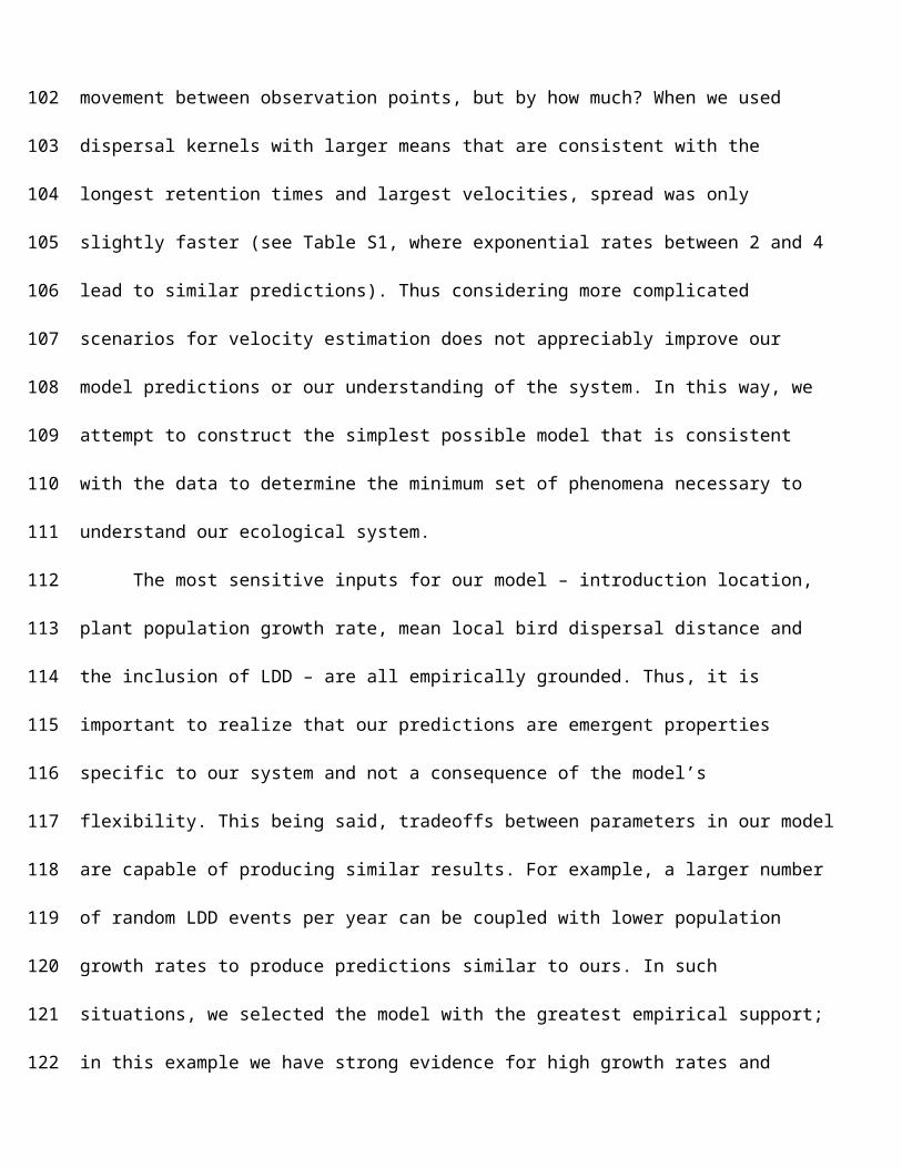
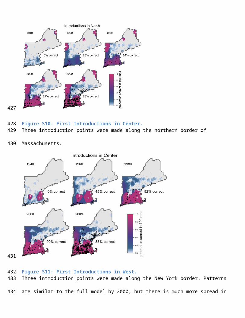
Throughout this appendix, white circles indicate introduction points; black dots are correctly predicted presences and

black circles indicate incorrectly predicted presences. The color scale indicates the proportion of model runs that

resulted in a presence, and is located to the right in each figure. The criterion for a correct prediction was that at least

50% of 100 model runs made the correct prediction. These are the same criteria described in the main text.

Figure S1: No plant population growth.Spread barely extends beyond introduction points.

240

241

242

243

244

245246

247

Figure S2: No local bird dispersal.Spread cannot occur continuously, only in discrete jumps provided by LDD.

Figure S3. No long distance dispersal.Local spread is similar to the full model, but remote areas are unreached throughout northern New England .

248249

250

251252

253

254

Figure S4. Homogeneous landscape.

This figure gives the high bittersweet growth rate scenario, where growth rate is the unweighted mean of all habitat

types (1.38). Bird and plant preferences were equal in all LULC classes. Note the symmetric pattern encircling each

introduction point (black dots).

This figure gives the low bittersweet growth rate scenario, which results when growth rates are weighted by

proportion of habitat. In fact, the weighted growth rate was 0.94, which clearly leads to extinction so we used a value

of 1.1.

255

256

257

258

259

260

261

262

263

Figure S5. Homogeneous landscape with no LDD. Bird and plant preferences were equal in all LULC classes. Note the symmetric pattern encircling each introduction

point (black dots), describing an unconstrained diffusion model.

264265

266

267268

Figure S6: Binary Landscape. The color scale indicates the proportion of model runs that resulted in a presence. Bird and plant preferences were

those in table 1. The dispersal kernel was exponential with rate 2.2. Note the symmetric pattern encircling each

introduction point (black dots), describing a diffusion model constrained by unsuitable habitat.

(Left) The binary landscape, where developed, agricultural and deciduous

forest are all classified as favorable habitat (green). Black circles denote

the observed presences from herbarium records.

269

270271

272

273

274

275

276

277

Figure S7: Random Landscape. Results from a representative randomly generated landscape, where the LULC proportions are the same as

observed, but their spatial alignment is randomized. The area of spread differs from the full model because the

geometry of the landscape is lost. The results are also much less consistent among model runs. However, the

proportion of runs that match herbarium predictions is much lower, because the random landscape does not

systematically direct the spread in the way that a real landscape, with larger clumps of similar habitat might.

Example of a random landscape

278

279280

281

282

283

284

285286

Figure S8: First Introductions in South.Three introduction points were made along the Connecticut coast. This differs from the full model because, although

the site near New Haven, Connecticut is used in both models, the full model has an introduction south of Boston and

another in southeastern New Hampshire.

Figure S9: First Introductions in North.Three introduction points were made along the Canadian border.

287288

289

290

291

292293

294

Figure S10: First Introductions in Center.Three introduction points were made along the northern border of Massachusetts.

Figure S11: First Introductions in West.Three introduction points were made along the New York border. Patterns are similar to the full model by 2000, but

there is much more spread in Vermont here.

295296

297

298299

300

301

Figure S12: First Introductions in East.Three introduction points were made along the east coast of New England.

Figure S13: Long term predictions Predictions appear to stabilize some time after 200 years. Except in Maine, the maximum spread has approximately

occurred within 200 years.

302303

304

305306

307

308

Figure S14: Random LDD Neighborhood 25 x 25Spread is more limited in the north than in the full model from 2000-2009, indicating that local bird dispersal was

ineffective in reaching this region over a span of 90 years. Interestingly, predictions are better in 1960-1980 than the

full model because all LDD event are constrained to land nearer to existing populations.

Figure S15: Random LDD Neighborhood 51 x 51Propagules reach remote areas sooner, however their infrequency, combined with the blocks of unfavorable

coniferous habitat in the north mean that spread is little affected. The main differences is that the agricultural areas in

northeastern Maine could now be reached (compared to the full model) from established populations further south,

however even this occurs rarely (not at all during this sample of 100 model runs). This dispersal neighborhood could

have been used in our model equally as well as the 51 x 51 grid cell neighborhood that we chose.

Figure S16: Start model in 1939Initiating the model in 1939 with the observed presences up until 1939. Spread is initially a bit slower compared to the

309310

311

312

313

314315

316

317

318

319

320

321322

full model (through 1980), but the pattern more closely resembles empirical observations in 1960. This suggests that

there may have been additional introduction along the Connecticut coast.

Figure S17: Start model in 1959Initiating the model in 1959 with the observed presences up until 1960. Similar to the model initiated in 1939, the

spread is initially slower than observed in the full model, but prediction accuracy increases in 1980 because the

location of populations in 1940 is sufficient to explain occurrence in 1980. It seems, however that there may have

been greater spread in 1980 than shown in this figure because results in 2000 suffer from under-prediction.

323

324

325

326327

328

329

330

Figure S18: Shorter Bird Dispersal and More LDDAssuming the starlings cannot disperse seeds a far (using a mean dispersal distance 1/3 that of the full model) and

that LDD is greater (5 events/ year, which sensitivity analyses shows is sufficient to saturate the New England by

1960) leads to a much patchier distribution of bittersweet that does not closely resemble historical records.

331

332333

334

335

336337

Appendix S3: Additional Data and Analysis

Table S3. Growth Rate and Habitat Use Data

Habitat % land-scape

% Starling’s

Time

Normalized Habitat Use

Index (% use / % landscape)

Seedling Survival

Plant Survival

Population Growth Rate

(λ)

Developed 15.3% 34.1% 0.39 49% 95-100% (8g)

2.1

Agricultural 16.5% 42.0% 0.44 64% 95-98% (6g)

1.5

Deciduous 62.9% 20.5% 0.06 66% 90-95% (2.5g)

1.4

Coniferous 5.3% 3.5% 0.11 43% 60-80% (1.5g)

0.5

Summary of data used to parameterize habitat use for European starlings and Oriental bittersweet. The proportion of

landscape was evaluated for the region where radio tracking was conducted (LaFleur 2006). Plant survival and mean

dry weight biomass was measured across replicate sites from a transplant experiment (seedlings: LaFleur

unpublished; adults: Leicht 2005). Bold values are model parameters estimated from data.

338

339340

341

342

343

344

345

346

Table S4: LULC ReclassificationsDefinitions of the reclassification scheme used to translate NOAA data for the model.

Original Class Description Revised Class

1 Unclassified Unsuitable

2 Developed, High Intensity Developed

3 Developed, Medium Intensity Developed

4 Developed, Low Intensity Developed

5 Developed, Open Space Developed

6 Cultivated Crops Agriculture/Scrub/Shrub

7 Pasture/Hay Agriculture/Scrub/Shrub

8 Grassland/Herbaceous Agriculture/Scrub/Shrub

9 Deciduous Forest Deciduous Forest

10 Evergreen Forest Coniferous Forest

11 Mixed Forest Coniferous Forest

12 Scrub/Shrub Agriculture/Scrub/Shrub

13 Palustrine Forested Wetland Unsuitable

14 Palustrine Scrub/Shrub Wetland Unsuitable

15 Palustrine Emergent Wetland (Persistent) Unsuitable

16 Estuarine Forested Wetland Unsuitable

17 Estuarine Scrub / Shrub Wetland Unsuitable

18 Estuarine Emergent Wetland Unsuitable

19 Unconsolidated Shore Unsuitable

20 Barren Land Unsuitable

21 Open Water Unsuitable

22 Palustrine Aquatic Bed Unsuitable

347348

Figure S19. Seed dispersal kernel estimates

We used radio tracking data to estimate local bird movements and banding recaptures to estimate larger scale

movements in conjunction with gut passage time to produce a seed dispersal kernel. Shown are three characteristic

seed retention times (that represent the range) coupled with both local and banding data. We produced a

conservative envelop around the kernel chosen for the model (dark line). The inset histogram shows the frequency

distribution of the distances traveled by starlings between banding and recapture over an intervals of two days or

less. The proportion of seeds deposited in each cell by the kernel chosen for the model (dark line) is shown along the

horizontal axis.

349350

351

352

353

354

355

356

357

358

359

Figure S20. Christmas Bird Counts for Potential Bittersweet Dispersers

Lines show Christmas Bird Counts for all birds known or suspected to be dispersers of Oriental bittersweet in New

England. Starlings vastly outnumbered all other species combined until 2006.

Figure S21. Consequences of eradication efforts in CT and RI

All populations were set to 0 in 2010 and immigrants from surrounding cells were allowed to repopulate the region.

360

361

362

363

364

365

366

Appendix S4: Model Code

######################################################################################################################## PART 1: Load Data ############################################################################################################################library(fields)#The following file contains a matrix called 'nelandscape'. the first two columns give coordinates of each cell on the 82 x 79 grid overlayed on the landscape with (1,1) being the southwest corner. The third column gives the LULC classification (1= water, 2=developed, 3=agriculture, 4=deciduous, 5=coniferous).print(load('nelandscape-appendix.RData')) #included data file from supplementary materials

######################################################################################################################## PART 2: Functions ############################################################################################################################

#FUNCTION FOR SIMULATIONScmstarling3dd=function(birddisp,landscape,lat0,long0, generations ,rate,plantprefs, carrying.cap,local.growth=TRUE, long.distance=TRUE,birds=TRUE,num.long.dist=1, recordtimes){ #birddisp:an array giving the probability of bird dispersal from each source cell to its respective bird dispersal neighborhood #landscape: matrix with columns giving x coords, y coords and LULC for each cell #lat0, long0: initial populations #generations: # of time steps to interate model #rate: 1/mean of the exponential dispersal kernel #plantprefs: a vector of population growth rates where the first element corresponds to LULC class 1, etc. #carrying.cap: carrying capacity in a single cell #local.growth: logical - include local growth? #long.distance: logical - include LDD? #birds: logical - include local bird dispersal? #num.long.dist: # LDD events/year #recordtimes: steps where a snapshot is take of population distribution

######### GENERAL ###################################################

init=cbind(long0, lat0)lat=max(landscape[,2])long=max(landscape[,1])

367

368369370371372373374375376377378379380381382383384385386387388389390391392393394395396397398399400401402403404405406

#record keeping variablesp=cbind(landscape,rep(0,lat*long)) #state variable for each cell timeseries=matrix(0,lat*long,length(recordtimes) )#to store snapshots of populationts.counter=1 ocean.sites=which(landscape[,3]==1) #good.sites=(1:length(landscape[,1]))[-ocean.sites]for(i in 1:nrow(init)){ #plants 1st seed(s)

p[which(landscape[,1]==init[i,1] & landscape[,2]==init[i,2]),4]=carrying.cap/2 }

########## DISPERSE SEEDS ############################ for (t in 1:generations){

#put a seed at Durham, NH in 1938 if(t==14){p[which(landscape[,1]==35 & landscape[,2]==28),4]=carrying.cap/2}

#LOCAL GROWTH ______________________________________________populated.sites=which(p[,4]>0)new.individuals=p[populated.sites,4]*(plantprefs[p[populated.sites,3]]-1)p[which(p[,3]==1) ,4]=0 #kill at unsuitable (ocean) sitesif(local.growth){

p[populated.sites,4]=ceiling(pmin(carrying.cap,p[populated.sites,4]+ as.numeric(plantprefs[p[populated.sites,3]]>=1)*new.individuals*pexp(.5,rate)+as.numeric(plantprefs[p[populated.sites,3]]<1)*new.individuals))

} #RANDOM LONG DISTANCE DISPERSAL _________________________________ if (long.distance){

for( i in 1:num.long.dist){ start.site=sample(which(p[,4]>=1),1) target.site=sample(which(p[,3]>1),1) while(length(target.site)<1){ #to ensure suitable sites found start.site=sample(which(p[,4]>=1),1) target.site=sample(which(p[,3]>1),1) }

newsite=sample(target.site,1) p[newsite,4]=min(carrying.cap,p[newsite,4]+1)

} } #BIRD DISPERSAL ______________________________________________________

#set up the # of offspring from each site emigrate=rep(0,length(p[,4])) emigrate[populated.sites]=new.individuals emigrate=pmax(0,emigrate) #get rid of sink pops

if( birds ){ num.bird.seeds=emigrate*(1-pexp(.5,rate)) for( k in which(round(num.bird.seeds,0)>0) ) { newsite=try(sample(subset(c(birddisp[,,2,k]),c(birddisp[,,2,k]>0)), round(num.bird.seeds[k],0),prob=subset(c(birddisp[,,1,k]),c(birddisp[,,2,k]>0)) ,replace=T),TRUE) #get the new sites

p[newsite,4]=pmin(carrying.cap, p[newsite,4]+1) #place the seeds in the new sites } } #_____________________________________________________________

#for specified time intervals, store the population matrix if ( sum(t==recordtimes)==1 ) { timeseries[ ,ts.counter]=p[1:6478 ,4] ts.counter=ts.counter+1 } } # time loop

407408409410411412413414415416417418419420421422423424425426427428429430431432433434435436437438439440441442443444445446447448449450451452453454455456457458459460461462463464

list(timeseries=timeseries) }

############################################################FUNCTION FOR DISPERSAL PROBABILITIES# determines the probability of being dispersed to each site from site i,j

dispersal.probs=function(landscape,maxdist,rate){#this function is always called outside of the cmstarling program

lat=max(landscape[,2])long=max(landscape[,1])

#avoids calculation at unsuitable sitesocean.sites=which(landscape[,3]==1) good.sites=(1:length(landscape[,1]))[-ocean.sites]

#make a matrix of distance weightsweights=matrix(0,2*maxdist+1,2*maxdist+1)center=c(maxdist+1,maxdist+1)for(i in seq(1,2*maxdist+1)){

for(j in seq(1,2*maxdist+1)){weights[i,j]=dexp( (i-center[1])^2 +(j-center[2])^2-.5,rate )

}}weights[center[1],center[2]]=0weights=weights/sum(weights)disp.matrix=array(0,c(nrow(weights),ncol(weights),2,lat*long))disp.matrix[,,1,good.sites]=weightsfor( k in good.sites){

xx=(landscape[k,1]-maxdist):(landscape[k,1]+maxdist)yy=(landscape[k,2]-maxdist):(landscape[k,2]+maxdist)

for(i in xx[xx>0 & xx<=long]){ for(j in yy[yy>0 & yy<=lat]){ disp.matrix[which(xx==i),which(yy==j),2,k]=which(landscape[,1]==i &

landscape[,2]==j) } }

}return(disp.matrix)

}

######################################################################################################################## PART 3: Sample Model Run ############################################################################################################################landscape=nelandscapebirdtime=c(0,.39,.44,.06,.11)#these correspond to the LULC types (ocean, developed, agriculture, deciduous, coniferous)

#MAKE DISPERSAL PROBABILITIES ---------------------------------------------maxdist=3 #sets size of local bird dispersal neighborhoodrate=3.5 #1/mean

#this calculates the distance weighted probabilities of dispersaldist.mat=dispersal.probs(landscape,maxdist,rate)

#this weights distances by bird habitat usea=0*dist.mat[,,1,]for( i in which(!landscape[,3]==1 & !landscape[,3]==0)) {

for( j in 1:(2*maxdist+1)){for(k in 1:(2*maxdist+1)){

if(!dist.mat[j,k,2,i]==0){a[j,k,i]=dist.mat[j,k,1,i]*birdtime[landscape[dist.mat[j,k,2,i],3]]

465466467468469470471472473474475476477478479480481482483484485486487488489490491492493494495496497498499500501502503504505506507508509510511512513514515516517518519520521522

}}

}a[,,i]=a[,,i]/sum(a[,,i])

}birddisp=dist.matbirddisp[,,1,]=a

#RUN MULTIPLE SIMULATIONS AND PRODUCE AVERAGE SURFACE----------------------reps=10 # number of replicate model runs. 100 runs were used in the manuscriptlat=max(landscape[,2]); long=max(landscape[,1]) d.reps=array(NA,c(lat*long,5,reps)) # to store output

#PARAMETERSplantprefs=c(0, 2.1, 1.5, 1.4, .5) #these correspond to the LULC types (water, developed, agriculture, deciduous, coniferous)recordtimes=c(21,41,61,81,90) # specify the time steps at which to record the results generations=90num.long.dist=1 # # of seeds per year for LDDlocal.growth=TRUElong.distance=TRUEbirds=TRUElong0=c(9,39); lat0=c(5,9) #initial conditionscarrying.cap=200 for(i in 1:reps){

d=cmstarling3dd(birddisp,landscape,lat0,long0,generations,rate,plantprefs, carrying.cap,local.growth,long.distance,birds,num.long.dist,recordtimes=recordtimes)

d.reps[,,i]=d$timeseriesprint(i)

}d.reps=ifelse(d.reps>0,1,0) #turn abundance predicitons in to presence/absenceavg.occupancy=matrix(NA,lat*long,5)for(i in 1:5){ avg.occupancy[,i]=apply(d.reps[,i,],1,mean) }

######################################################################################################################## PART 4: Plot Results #################################################################################################################################years=c(1940,1960,1980,2000,2009) #labels for plottingthreshold=.50avg.occupancy[landscape[,3]==1,]=2.2 # a placeholder for water so the plot looks prettyzc=array(0,c(82,79,5)) #create a grid for use in 'image' functionfor(i in 1:nrow(landscape)){ zc[landscape[i,1],landscape[i,2],]=avg.occupancy[i,] }par(oma=c( 1,1,3,5),mfrow=c(2,3),mar=c(0,0,0,0)) for(i in 1:5){

image(1:82,1:79,zc[,,i],col=colorRampPalette(c('grey90','lightsteelblue2', 'steelblue4','darkslateblue','violetred3', 'white'),bias=3)(100), col.axis='white',xaxt='n',yaxt='n',xlim=c(-1,84),ylim=c(-1,81),bty='n')

text(15,70,years[i],cex=1.7)points(c(long0,35),c(lat0,28),cex=1.2,lwd=2,col='grey90') #introduction points

}par(oma=c(2,0,8,18))image.plot(legend.only=T,zlim=c(0,1),col=colorRampPalette(c('grey90','lightsteelblue2','steelblue4','darkslateblue','violetred3'),bias=3)(100),legend.width=8)

523524525526527528529530531532533534535536537538539540541542543544545546547548549550551552553554

555556557558559560561562563564565566567568569570571572573574575576577578

579