appendix j. wastewater dispersion modelling study (rps 2017c)

Appendix J.

Wastewater dispersion modelling study (RPS 2017c)

apasa.com.au

ConocoPhillips Barossa Project

Wastewater Dispersion Modelling

Prepared by:

RPS

Suite E1, Level 4

140 Bundall Rd

Bundall, QLD 4217

T: +61 7 5574 1112

F: +61 8 9211 1122

E: [email protected]

Client Manager: Dr Sasha Zigic

Report Number: MAQ0540J.000

Version / Date: Rev1/14 March 2017

Prepared for:

CONOCOPHILLIPS AUSTRALIA

Dr Brenton Chatfield

53 Ord Street

West Perth WA 6005

Mail: PO Box 1102

West Perth WA 6872

T: +61 8 6363 2666

E: [email protected]

W: www.conocophillips.com.au

ConocoPhillips Barossa Project Wastewater Dispersion Modelling

MAQ0540J; Rev1/14 March 2017 Page ii

Document Status

Version Purpose of Document Original Review Review Date

Draft A Issued for client review Dr Ryan Dunn Dr Sasha Zigic 28/2/2017

Rev 0 Issued for client review Dr Ryan Dunn Dr Sasha Zigic 28/2/2017

Rev 1 Issued to client Dr Sasha Zigic 14/3/2017

Approval for Issue

Name Signature Date

Dr Sasha Zigic

14/3/2017

DISCLAIMER:

This report has been issued to the client under the agreed schedule and budgetary requirements and

contains confidential information that is intended only for use by the client and is not for public circulation,

publication, nor any third party use without the approval of the client.

Readers should understand that modelling is predictive in nature and while this report is based on

information from sources that RPS considers reliable, the accuracy and completeness of said information

cannot be guaranteed. Therefore, RPS, its directors, and employees accept no liability for the result of any

action taken or not taken on the basis of the information given in this report, nor for any negligent

misstatements, errors, and omissions. This report was compiled with consideration for the specified client's

objectives, situation, and needs. Those acting upon such information without first consulting RPS, do so

entirely at their own risk.


MAQ0540J; Rev1/14 March 2017 Page iii

Contents

1.0 INTRODUCTION ...................................................................................................................................... 1

1.1 Project background ..................................................................................................................... 1

2.0 DISPERSION MODELLING ..................................................................................................................... 2

2.1 Near-field model ........................................................................................................................... 2

2.1.1 Description ...................................................................................................................... 2

2.1.2 Model setup .................................................................................................................... 3

2.2 Interannual variability .................................................................................................................. 5

2.3 Development of regional current data ....................................................................................... 7

2.3.1 Tidal currents .................................................................................................................. 7

2.3.2 Ocean currents ............................................................................................................... 9

2.3.3 Tidal and current model validation ................................................................................ 15

2.4 Environmental reporting criteria .............................................................................................. 21

3.0 MODELLING RESULTS ........................................................................................................................ 22

4.0 KEY FINDINGS ...................................................................................................................................... 31

5.0 REFERENCES ....................................................................................................................................... 31

6.0 APPENDICES ........................................................................................................................................ 34

6.1 Appendix A. Predicted minimum plume dilution .................................................................... 34


MAQ0540J; Rev1/14 March 2017 Page iv

Tables

Table 1 Barossa offshore development area wastewater dispersion modelling study release location ............ 1

Table 2 Wastewater discharge and pipe configuration characteristics summary .............................................. 4

Table 3 Water temperature and salinity model inputs ........................................................................................ 4

Table 4 Seasonal ambient percentile current speeds, strength and predominant direction as a function of water depth at the release location ..................................................................................................................... 4

Table 5 Statistical evaluation between measured water levels and HYDROMAP predicted water levels at CP1 ................................................................................................................................................................... 16

Table 6 Statistical evaluation between averaged measured currents and HYCOM ocean current and HYDROMAP tidal current at CP1, CP2 and CP3 at varying water depths (July 2014 to March 2015) ........... 20

Table 7 Maximum distance from wastewater discharge release location to achieve defined average dilution levels for each flow rate, season and current strength ..................................................................................... 23

Table 8 Predicted wastewater plume characteristics upon either reaching the sea surface or achieving 1:5,000 average dilution for the commissioning stage (96.1 m3/day) ............................................................... 24

Table 9 Predicted wastewater plume characteristics upon either reaching the sea surface or achieving 1:5,000 average dilution for the operation stage (45.0 m3/day) ....................................................................... 24

Table 10 Maximum distance from wastewater discharge release location to achieve defined minimum dilution levels for each flow rate, season and current strength ..................................................................................... 35

Figures

Figure 1 Map of the Barossa offshore development area wastewater modelling study release location. ......... 2

Figure 2 Monthly values of the SOI 2005-2014. Sustained positive values indicate La Niña conditions, while sustained negative values indicate El Niño conditions (Data sourced from Australian Bureau of Meteorology 2015). .................................................................................................................................................................. 5

Figure 3 Annual surface ocean current rose plots within the Barossa offshore development area. Derived from analysis of HYCOM ocean data for the years 2005–2014. The colour key shows the current speed (m/s), the compass shows the direction and the length of the wedge gives the percentage of the record for a particular speed and direction combination. ....................................................................................................... 6

Figure 4 Map showing the extent of the tidal model grid. Note, darker regions indicate higher grid resolution. 8

Figure 5 Zoomed in map showing the tidal model grid), illustrating the resolution sub-gridding in complex areas (e.g. islands, banks, shoals or reefs) ........................................................................................................ 8

Figure 6 Map showing the bathymetry of the tidal model grid ............................................................................ 9

Figure 7 Seasonal surface current rose plots adjacent to the release location. Data was derived from the HYCOM ocean currents for years, 2010, 2012 and 2014. The colour key shows the current magnitude (m/s), the compass direction provides the current direction flowing TOWARDS and the length of the wedge gives the percentage of the record for a particular speed and direction combination. .............................................. 10

Figure 8 Modelled HYCOM surface ocean currents on the 6th February 2012, summer conditions (upper image) and 11th May 2012, winter conditions (lower image). Derived from the HYCOM ocean hindcast model (Note: for image clarity only every 2nd vector is displayed). ............................................................................ 11

Figure 9 Monthly surface current rose plots adjacent to the model release location. Derived from analysis of HYCOM ocean data and tidal data for 2010 (La Niña year). The colour key shows the current speed (m/s), the compass shows the direction and the length of the wedge gives the percentage of the record for a particular speed and direction combination. ..................................................................................................... 12

Figure 10 Monthly surface current rose plots adjacent to the model release location. Derived from analysis of HYCOM ocean data and tidal data for 2012 (neutral year). The colour key shows the current speed (m/s), the


MAQ0540J; Rev1/14 March 2017 Page v

compass shows the direction and the length of the wedge gives the percentage of the record for a particular speed and direction combination. ..................................................................................................................... 13

Figure 11 Monthly surface current rose plots adjacent to the model release location. Derived from analysis of HYCOM ocean data and tidal data for 2014 (El Niño year). The colour key shows the current speed (m/s), the compass shows the direction and the length of the wedge gives the percentage of the record for a particular speed and direction combination. ..................................................................................................... 14

Figure 12 Locations of the CP1, CP2 and CP3 current meter moorings and the wind station ........................ 15

Figure 13 Comparison of measured and modelled water levels at CP1 .......................................................... 16

Figure 14 Comparison of predicted and measured current roses at CP1 from 9th July 2014 to 21st March 2015 .................................................................................................................................................................. 17

Figure 15 Comparison of predicted and measured current roses at CP2 from 10th July 2014 to 20st March 2015 .................................................................................................................................................................. 18

Figure 16 Comparison of predicted and measured current roses at CP3 from 9th July 2014 to 21st March 2015. ................................................................................................................................................................. 19

Figure 17 Near-field average temperature and dilution results for constant weak, medium and strong summer currents (96.1 m3/d flow rate) ........................................................................................................................... 25

Figure 18 Near-field average temperature and dilution results for constant weak, medium and strong transitional currents (96.1 m3/d flow rate) ......................................................................................................... 26

Figure 19 Near-field average temperature and dilution results for constant weak, medium and strong winter currents (96.1 m3/d flow rate) ........................................................................................................................... 27

Figure 20 Near-field average temperature and dilution results for constant weak, medium and strong summer currents (45.0 m3/d flow rate) ........................................................................................................................... 28

Figure 21 Near-field average temperature and dilution results for constant weak, medium and strong transitional currents (45.0 m3/d flow rate) ......................................................................................................... 29

Figure 22 Near-field average temperature and dilution results for constant weak, medium and strong winter currents (45.0 m3/d flow rate) ........................................................................................................................... 30


MAQ0540J; Rev1/14 March 2017 Page 1

1.0 Introduction

1.1 Project background

ConocoPhillips Australia Exploration Proprietary (Pty) Limited (Ltd.) (ConocoPhillips), as proponent on behalf of

the current and future co-venturers, is proposing to develop natural gas resources in the Timor Sea into high

quality products in a safe, reliable and environmentally responsible manner. The Barossa Area Development

(herein referred to as the “project”) is located in Commonwealth waters within the Bonaparte Basin, offshore

northern Australia, and is approximately 300 kilometres (km) north of Darwin, Northern Territory (NT).

The development concept of the gas resource includes a floating production storage and offloading (FPSO)

facility and a gas export pipeline that are located in Commonwealth jurisdictional waters. The FPSO facility will

be the central processing facility to stabilise, store and offload condensate, and to treat, condition and export

gas. The extracted lean dry gas will be exported through a new gas export pipeline that will tie into the existing

Bayu-Undan to Darwin gas export pipeline. The lean dry gas will then be liquefied for export at the existing

ConocoPhillips operated Darwin Liquefied Natural Gas facility at Wickham Point, NT.

The FPSO facility will be required to discharge wastewater (includes treated sewage, greywater and deck

drainage waters) to the marine environment. The wastewater contains constituents such as oil/grease,

suspended solids and coliform bacteria, into the receiving environment.

As the wastewater will contain constituents exceeding levels those of the ambient marine waters,

ConocoPhillips commissioned RPS to conduct a dispersion modelling study. The main objective of the study

was to assess the near-field mixing and dilution zones for the wastewater discharge during the two stages

under static weak, medium and strong current strengths. The coordinate of the indicative release location is

presented in Table 1 and graphically in Figure 1. The purpose of the modelling was to assist in understanding

the potential area that may be influenced by the routine discharge of wastewater based on the engineering

information available in the early stage of the project design phase.

The potential area that may be influenced by the wastewater discharge stream was assessed for three distinct

seasons; (i) summer (December to the following February), (ii) the transitional periods (March and September to

November) and (iii) winter (April to August). This approach assists with identifying the environmental values and

sensitivities that would be at risk of exposure on a seasonal basis.

The closest environmental values and sensitivities to the modelled release location are submerged shoals and

banks including Lynedoch Bank (70 km to the south-east), Evans Shoal (64 km to the west) and Tassie Shoal

(74 km to the south-west).

Table 1 Barossa offshore development area wastewater dispersion modelling study release location

Release location Latitude Longitude Water depth (mLAT)

Barossa offshore development area

release location 9° 52’ 35.8” S 130° 11’ 8.4” E ~230



Figure 1 Map of the Barossa offshore development area wastewater modelling study release location.

2.0 Dispersion modelling

Due to the low flow rate and characteristics of the wastewater near-field modelling was only required to assess

the very localised zone of influence.

The near-field zone is defined by the region where the levels of mixing and dilution are controlled by the plume’s

initial jet momentum and the buoyancy flux, resulting from the density difference. When the plume encounters a

boundary such as the water surface, seabed or density stratification layer, the near-field mixing is complete and

the far-field mixing begins.

2.1 Near-field model

2.1.1 Description

The near-field mixing of the wastewater discharge stream was predicted using the fully three-dimensional flow

model, Updated Merge (UM3). The UM3 model is used for simulating single and multi-port submerged

discharges and is part of the Visual Plumes suite of models maintained by the United States Environmental

Protection Agency (Frick et al. 2003).

The UM3 model has been extensively tested for various discharges and found to predict the observed dilutions

more accurately (Roberts and Tian 2004) than other near-field models (e.g. RSB or CORMIX).



In this Lagrangian model, the equations for conservation of mass, momentum, and energy are solved at each

time-step, giving the dilution along the plume trajectory. To determine the growth of each element, UM3 uses

the shear (or Taylor) entrainment hypothesis and the projected-area-entrainment hypothesis. The flows begin

as round buoyant jets issuing from one side of the diffuser and can merge to a plane buoyant jet (Carvalho et al.

2002). Model output consists of plume characteristics, including centerline dilution, rise-rate, width, centreline

height and diameter of the plume. Dilution is reported as the “effective dilution”, which is the ratio of the initial

concentration to the concentration of the plume at a given point, following Baumgartner et al. (1994).

2.1.2 Model setup

The discharge characteristics for the wastewater during the commissioning and operational stages are

summarised in Table 20. The wastewater was modelled as a discharge 10 m below the water surface through a

single outlet, and was anticipated to have a salinity and temperature of 1 part per thousand (ppt) and 25°C,

respectively, during commissioning and operational stages. The modelled initial oil/grease concentration was 30

mg/L, the initial total suspended solids concentration was 50 milligrams per litre (mg/L) and the initial coliform

bacteria concentration was 250 col/100 mL, for both stages. As detailed engineering design of the FPSO was

yet to be undertaken at the time the modelling was commissioned, the concentrations of the wastewater

constituents were based on those publically available in Shell’s Prelude Floating LNG Environmental Impact

Statement (Shell 2009).

Additional input data used to setup the near-field model included range of current speeds, water temperature

and salinity as a function of depth. Defining the water temperature and salinity is important to correctly replicate

the buoyancy of the diluting plume. The buoyancy dynamics in this case will be dominated by the salinity

differences between the wastewater plume and receiving waters.

Table 3 presents the measured water temperature and salinity data collected by Fugro Survey Pty Ltd (Fugro)

(2015) as part of the Barossa marine studies program. The minimum water temperature at 30 m below mean

sea level (BMSL) was used as it represents the most conservative conditions considering water temperature

varies with depth and would be warmer at the surface in comparison to temperatures at 30 m.

Table 4 presents the 5th, 50th and 95th percentiles of current speeds, which reflect contrasting dilution and

advection cases:

▪ 5th percentile current speed: weak currents, low dilution and slow advection

▪ 50th percentile (median): medium current speed, moderate dilution and advection

▪ 95th percentile current speed: strong currents, high dilution and rapid advection to nearby areas.

The 5th percentile, 50th percentile (median) and 95th percentile values are referenced as weak, medium and

strong current speeds, respectively.



Table 2 Wastewater discharge and pipe configuration characteristics summary

Parameter Value/design

Flow rate (m3/day) Commissioning flow rate: 96.1

Operational flow rate: 45.0

Outlet pipe internal diameter (m) 0.03

Pipe orientation Vertically downward

Depth of pipe below sea surface (m) 10

Discharge salinity (ppt) 1

Discharge temperature (oC) 25

Discharge oil-in-water concentration (mg/L) 30

Table 3 Water temperature and salinity model inputs

Parameter Season

Summer Transitional Winter

Ambient minimum water temperature (oC) (30 m BMSL) 25.4 24.7 26.3

Ambient mean salinity (Practical Salinity Units (PSU)) (30 m BMSL) 34.1 33.6 33.6

Table 4 Seasonal ambient percentile current speeds, strength and predominant direction as a function of water depth at the release location

Depth

below the

water

surface

(m)

Parameter

Reporting

current

strength

Season

Summer Transitional Winter

Speed

(m/s)

Predominant

direction

Speed

(m/s)

Predominant

direction

Speed

(m/s)

Predominant

direction

0

5th percentile Weak 0.04

East

0.05

West-south-

west

0.03

South-west

50th

percentile Medium 0.11 0.14 0.11

95th

percentile Strong 0.27 0.29 0.27

10


East

0.03

South-west

0.04

South-west

50th


95th


20


East-south-

east

0.03

South-west

0.03

South-west

50th


95th




2.2 Interannual variability

The region is strongly affected by the strength of the Indonesian Throughflow, which fluctuates from one year to

the next due to the exchange between the Pacific and Indian Oceans. Therefore, in order to examine the

potential range of variability, the Southern Oscillation Index (SOI) data sourced from the Australian Bureau of

Meteorology was used to identify interannual trends for the last 10 years (2005–2014). The SOI broadly defines

neutral, El Niño (sustained negative values of the SOI below −8 often indicate El Niño episodes) and La Niña

(sustained positive values of the SOI above +8 are typical of La Niña episodes) conditions based on differences

in the surface air-pressure between Tahiti on the eastern side of the Pacific Ocean and Darwin (Australia), on

the western side (Rasmusson and Wallace 1983, Philander 1990). El Niño episodes are usually accompanied

by sustained warming of the central and eastern tropical Pacific Ocean and a decrease in the strength of the

Pacific trade winds. La Niña episodes are usually associated with converse trends (i.e. increase in strength of

the Pacific trade winds).

Figure 2 shows the SOI monthly values and Figure 3 shows the surface ocean current roses for the period

2004–2013 at the proposed release location. Each current rose diagram provides an understanding of the

speed, frequency and direction of currents, over the given year:

▪ Current speed – speed is divided into segments of different colour, ranging from 0 to greater than 1 m/s.

Speed intervals of 0.2 m/s are used. The length of each coloured segment is relative to the proportion of

currents flowing within the corresponding speed and direction;

▪ Frequency – each of the rings on the diagram corresponds to a percentage (proportion) of time that currents

were flowing in a certain direction at a given speed;

▪ Direction – each diagram shows currents flowing towards particular directions, with north at the top of the

diagram.

Based on the combination of the SOI assessment and surface ocean currents, 2010 was selected as a

representative La Niña year, 2012 was selected as a representative neutral year, and 2014 was selected as an

El Niño year.

Figure 2 Monthly values of the SOI 2005-2014. Sustained positive values indicate La Niña conditions, while sustained negative values indicate El Niño conditions (Data sourced from Australian Bureau of Meteorology 2015).



Figure 3 Annual surface ocean current rose plots within the Barossa offshore development area. Derived from analysis of HYCOM ocean data for the years 2005–2014. The colour key shows the current speed (m/s), the

compass shows the direction and the length of the wedge gives the percentage of the record for a particular speed and direction combination.



2.3 Development of regional current data

The project is located within the influence of the Indonesian Throughflow, a large scale current system

characterised as a series of migrating gyres and connecting jets that are steered by the continental shelf. This

results in sporadic deep ocean events causing surface currents to exceed 1.5 m/s (approximately 3 knots).

While the ocean currents generally flow toward the southwest, year-round, the internal gyres generate local

currents in any direction. As these gyres migrate through the area, large spatial variations in the speed and

direction of currents will occur at a given location over time.

The influence of tidal currents is generally weaker in the deeper waters and greatest surrounding regional reefs

and islands. Therefore, it was critical to include the influence of both types of currents (ocean and tides) to

rigorously understand the likely discharge characteristics in the project’s area of influence.

A detailed description of the tidal and ocean current data inputted into the model is provided below.

2.3.1 Tidal currents

The tidal circulation was generated using RPS’s advanced ocean/coastal model, HYDROMAP. The

HYDROMAP model has been thoroughly tested and verified through field measurements throughout the world

over the past 26 years (Isaji and Spaulding 1984; Isaji et al. 2001; Zigic et al. 2003). In addition, HYDROMAP

tidal current data has been used as input to forecast (in the future) and hindcast (in the past) condensate spills

in Australian waters and forms part of the Australian National Oil Spill Emergency Response System operated

by the Australian Maritime Safety Authority (AMSA).

HYDROMAP employs a sophisticated sub-gridding strategy, which supports up to six levels of spatial resolution,

halving the grid cell size as each level of resolution is employed. The sub-gridding allows for higher resolution of

currents within areas of greater bathymetric and coastline complexity, and/or of particular interest to a study.

The numerical solution methodology follows that of Davies (1977a, 1977b) with further developments for model

efficiency by Owen (1980) and Gordon (1982). A more detailed presentation of the model can be found in Isaji

and Spaulding (1984), Isaji et al. (2001) and Owen (1980).

1.1.1.1 Tidal grid setup

The HYDROMAP tidal grid was established over a domain that extended approximately 2,400 km (east–west)

by 1,575 km (north–south) (Figure 4). Computational cells were square, with sizes varying from 8 km in the

open waters down to 1 km in some areas, to more accurately resolve flows along the coastline, around islands

and reefs, and over more complex bathymetry (Figure 5).

Bathymetry used in the model was obtained from multiple sources (Figure 6). This included bathymetry data

sourced from the Geoscience Australia database and commercially available digitised navigation charts.



Figure 4 Map showing the extent of the tidal model grid. Note, darker regions indicate higher grid resolution.

Figure 5 Zoomed in map showing the tidal model grid), illustrating the resolution sub-gridding in complex areas (e.g. islands, banks, shoals or reefs)



Figure 6 Map showing the bathymetry of the tidal model grid

1.1.1.2 Tidal data

The ocean boundary data for the regional model was obtained from satellite measured altimetry data

(TOPEX/Poseidon 7.2) which provided estimates of the eight dominant tidal constituents at a horizontal scale of

approximately 0.25 degrees. Using the tidal data, surface heights were firstly calculated along the open

boundaries, at each time step in the model.

The Topex-Poseidon satellite data is produced and quality controlled by the National Aeronautics and Space

Administration (NASA). The satellites, equipped with two highly accurate altimeters that are capable of taking

sea level measurements to an accuracy of less than 5 cm, measured oceanic surface elevations (and the

resultant tides) for over 13 years (1992–2005; see Fu et al., 1994; NASA/Jet Propulsion Laboratory 2013a;

2013b). In total these satellites carried out 62,000 orbits of the planet. The Topex-Poseidon tidal data has been

widely used amongst the oceanographic community, being the subject of more than 2,100 research publications

(e.g. Andersen 1995, Ludicone et al. 1998, Matsumoto et al. 2000, Kostianoy et al. 2003, Yaremchuk and

Tangdong 2004, Qiu and Chen 2010). As such the Topex/Poseidon tidal data is considered accurate for this

study.

2.3.2 Ocean currents

Data describing the flow of ocean currents was obtained from the Hybrid Coordinate Ocean Model (HYCOM)

(see Chassignet et al. 2007, 2009), which is operated by the HYCOM Consortium, sponsored by the Global

Ocean Data Assimilation Experiment (GODAE). HYCOM is a data-assimilative, three-dimensional ocean model

that is run as a hindcast, assimilating time-varying observations of sea surface height, sea surface temperature

and in-situ temperature and salinity measurements (Chassignet et al. 2009). The HYCOM predictions for drift

currents are produced at a horizontal spatial resolution of approximately 8.25 km (1/12th of a degree) over the

region, at a frequency of once per day. HYCOM uses isopycnal layers in the open, stratified ocean, but uses the



layered continuity equation to make a dynamically smooth transition to a terrain following coordinate in shallow

coastal regions, and to zlevel coordinates in the mixed layer and/or unstratified seas.

For this modelling study, the HYCOM hindcast currents were obtained for the years 2010 to 2014 (inclusive).

Figure 7 shows the seasonal surface current roses distributions adjacent to the release location by combining

2010, 2012 and 2014. The data shows that the surface current speeds and directions varied between seasons.

In general, during transitional conditions (March, April and September to November) currents were shown to

have the strongest average speed (average speed of 0.15 m/s with a maximum of 0.39 m/s) and tended to flow

to the west-southwest. During summer (December to February) and winter (May to August) conditions the

current flow was more variable though mostly toward the east and west, respectively. The average and

maximum speeds during summer was 0.11 m/s and 0.41 m/s, respectively. During winter the average was 0.13

m/s and 0.47 m/s as the maximum.

Figure 7 Seasonal surface current rose plots adjacent to the release location. Data was derived from the HYCOM ocean currents for years, 2010, 2012 and 2014. The colour key shows the current magnitude (m/s), the compass

direction provides the current direction flowing TOWARDS and the length of the wedge gives the percentage of the record for a particular speed and direction combination.

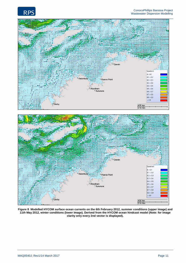
Figure 8 shows example screenshots of the predicted HYCOM ocean currents during summer and winter

conditions. The colours of the arrows indicate current speed (m/s).

In addition, Figure 9 to Figure 11 show the monthly surface current rose plots adjacent to the release location

for 2010, 2012 and 2014, respectively. The data is derived by combining the ocean currents and tidal currents.



Figure 8 Modelled HYCOM surface ocean currents on the 6th February 2012, summer conditions (upper image) and 11th May 2012, winter conditions (lower image). Derived from the HYCOM ocean hindcast model (Note: for image

clarity only every 2nd vector is displayed).



Figure 9 Monthly surface current rose plots adjacent to the model release location. Derived from analysis of HYCOM ocean data and tidal data for 2010 (La Niña year). The colour key shows the current speed (m/s), the




Figure 10 Monthly surface current rose plots adjacent to the model release location. Derived from analysis of HYCOM ocean data and tidal data for 2012 (neutral year). The colour key shows the current speed (m/s), the




Figure 11 Monthly surface current rose plots adjacent to the model release location. Derived from analysis of HYCOM ocean data and tidal data for 2014 (El Niño year). The colour key shows the current speed (m/s), the




2.3.3 Tidal and current model validation

Fugro measured water levels and currents (speed and directions) at three locations within the Barossa offshore

development area as part of the Barossa marine studies program (Figure 12, Fugro 2015). The measured data

from the survey was made available to validate the predicted currents, which corresponds to the three identified

seasons of the region (i.e. summer (December to February), transitional (March and September to November)

and winter (April to August)).

Figure 12 Locations of the CP1, CP2 and CP3 current meter moorings and the wind station

As an example, Figure 13 shows a comparison between the measured and predicted water levels at CP1 from

28 October 2014 to 14 March 2015. The figure shows a strong agreement in tidal amplitude and phasing

throughout the entire deployment duration at the CP1 location.

To provide a statistical quantification of the model accuracy, comparisons were performed by determining the

deviations between the predicted and measured data. As such, the root-mean square error (RMSE), root-mean

square percentage (RMS %) and relative mean absolute error (RMAE) were calculated. Qualification of the

RMAE ranges are reported in accordance with Walstra et al. (2001).

Table 5 shows the model performance when compared with measured water levels at CP1 from 28 October to

14 March 2015. According to the statistical measure, the HYDROMAP tidal model predictions were in very

good agreement with the measured water levels at CP1.



Figure 13 Comparison of measured and modelled water levels at CP1

Table 5 Statistical evaluation between measured water levels and HYDROMAP predicted water levels at CP1

Site RMSE (m) RMS (%) RMAE RMAE qualification

Mooring CP1 0.061 0.03 0.05 Very good

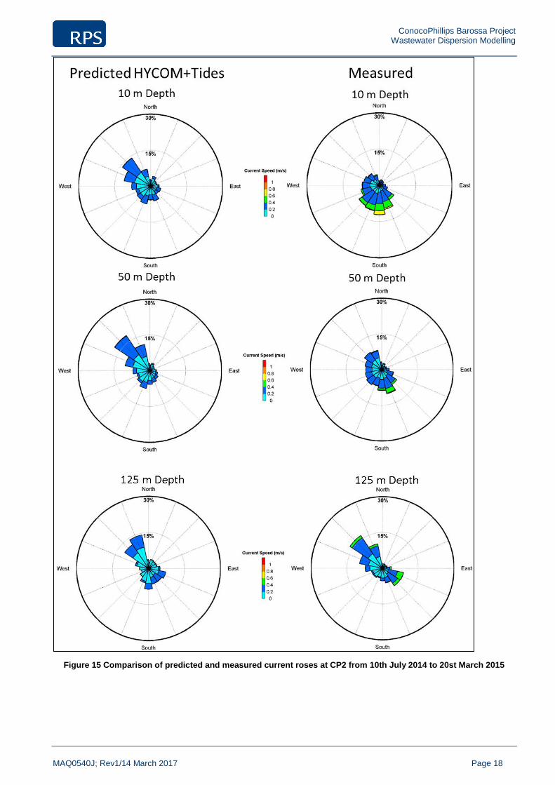
In addition, the HYCOM ocean currents combined with HYDROMAP tidal currents were compared to the

measured current speed and directions from the CP1, CP2 and CP3 moorings. Figure 14 to Figure 16 show

current comparison plots of the measured and predicted currents at each location for a range of depths (10 m,

50 m and 125 m BMSL) to highlight the differences between the wind-influenced surface layers and the mid

water column.



Figure 14 Comparison of predicted and measured current roses at CP1 from 9th July 2014 to 21st March 2015



Figure 15 Comparison of predicted and measured current roses at CP2 from 10th July 2014 to 20st March 2015



Figure 16 Comparison of predicted and measured current roses at CP3 from 9th July 2014 to 21st March 2015.

Overall, there was a good agreement between the predicted and measured currents at each site and depth. The

model predictions were also able to recreate the two-layer flow which can be seen in the measured data and the



reduction in current speeds as function of depth. From 10 m down to approximately 100 m below mean sea

level (BMSL) the currents generally flowed south-east, with little variation due to tidal changes. The model

predictions replicated this behaviour. Below 100 m, the influence of the tides became more pronounced, rotating

between a south-eastward flow and a north-westward flow with the turning of the tide. Both tidal-scale and

large-scale fluctuations in currents were typically reproduced at a similar magnitude and timing.

There was some divergence between the predicted and measured currents, mostly between data from July to

October inclusive, due to the occurrence of solitons (or high frequency internal waves that can produce

unusually high currents) which was highlighted by Fugro (2015). Despite these variations, the statistical

comparisons between the measured and predicted current speeds indicate a reasonable to very good

agreement (Table 6). Therefore, it can be concluded it is a good comparison and that the predicted current data

reliably reproduced the complex conditions within the Barossa offshore development area and surrounding

region. The RPS APASA (2015) model validation report provides a more detail regarding the tide and current

comparison.

In summary, the Fugro (2015) data provides information specifically for the Barossa offshore development area

and is considered the best available and most accurate data for this particular region. This data has been

provided and reviewed by RPS to confirm predicted currents applied are accurate. As a result, the current data

used herein is considered best available and highly representative of the characteristics influencing the marine

environment in the Barossa offshore development area.

Table 6 Statistical evaluation between averaged measured currents and HYCOM ocean current and HYDROMAP tidal current at CP1, CP2 and CP3 at varying water depths (July 2014 to March 2015)

Site Depth (m BMSL) RMSE (m/s) Measured peak

value (m/s) RMSE (%)

RMAE

qualification

Mooring CP1

10 0.14 0.71 20 Good

50 0.14 0.63 22 Very good

125 0.13 0.61 22 Very good

Mooring CP2

10 0.16 0.82 19 Reasonable

50 0.14 0.81 17 Good

125 0.16 0.72 22 Reasonable

Mooring CP3

10 0.15 0.88 18 Very good

50 0.14 0.78 18 Very good

125 0.13 0.60 21 Very good



2.4 Environmental reporting criteria

The following environmental criteria were used for the modelling study.

Dilution contours

The near-field modelling results are presented as dilutions levels to enable direct comparison of the minimum

dilutions for various wastewater constituents, including those that have yet to be confirmed or determined.

Dilution intervals of 1:10, 1:50, 1:100, 1:500, 1:1,000, 1:2,000, 1:3,333 and 1:5,000 were reported and are

considered very conservative in terms of the dilutions.



3.0 Modelling results

The results were carefully assessed to better understand the change in temperature and dilution of the

wastewater plume. Due to the low wastewater flow rates during both the commissioning (96.1 m3/day) and

operation (45.0 m3/day) stages, the wastewater plume was predicted to plunge less than 0.8 m below the

discharge pipe under all current conditions (weak, medium and strong). Following the discharge and initial

dilution, the wastewater plume was pushed horizontally from the discharge pipe while rising through the water

column due to density differences with the receiving waters.

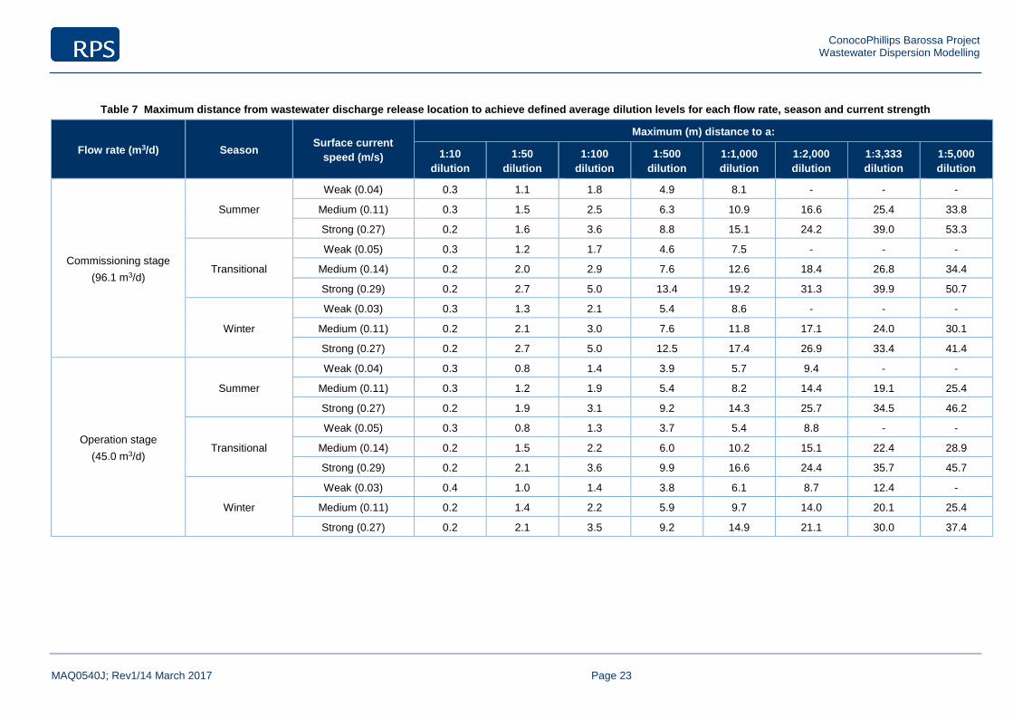
Table 7 presents the predicted maximum distance from the release location to achieve a given average dilution

for each flow rate (commissioning and operation) and season (summer, transitional and winter). In summary,

dilution rates of 1:100 and 1:5,000 were achieved within 5.0 m and 53.3 m, respectively, from the release

location due to the low flow rates and buoyancy of the wastewater discharge stream. Appendix A provides a

summary of the maximum distance from the release location to achieve a given minimum dilution (i.e. dilution of

plume centreline) for each flow rate and season.

During commissioning (96.1 m3/day), a 1:100 dilution was achieved within 2.1 m, 3.0 m and 5.0 m from the

release location during the constant weak, medium and strong current conditions, respectively. Additionally, the

1:100 dilution extended a maximum distance of 3.6 m, 5.0 m and 5.0 m from the release location under

summer, transitional and winter conditions, respectively (Table 7).

For the operational stage (45.0 m3/day), a 1:100 dilution was predicted to be achieved within 1.4 m, 2.2 m and

3.6 m from the release location during the constant weak, medium and strong current conditions, respectively.

Additionally, during the operational stage, the 1:100 dilution extended a maximum distance of 3.1 m, 3.6 m and

3.5 m from the release location under summer, transitional and winter conditions, respectively (Table 7).

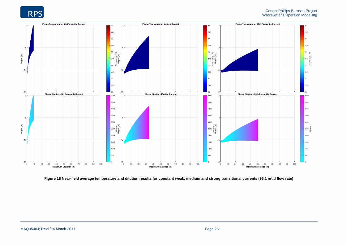
Table 8 and Table 9 present the plume characteristics upon either reaching the sea surface or achieving

1:5,000 average dilution for the two stages. There were no differences observed between final plume

temperature and ambient water temperature for both stages and all current speeds.

Based on the commissioning flow rate, the maximum horizontal distance to achieve the 1:5,000 average dilution

by the plume was 34.4 m and 53.3 m under constant medium and strong current conditions, respectively (Table

8). The corresponding minimum dilution was 1:1,267 and 1:1,236 under constant medium and strong current

conditions, respectively. During constant weak currents, the plume reached the sea surface and the average

dilution achieved was < 1:1,637, up to 10.7 m from the release location. The plume diameter at the sea surface

was < 7.3 m, <8.7 m and <5.4 m under constant weak, medium and strong current conditions, respectively

(Table 8).

Results for the operational flow rate, showed the maximum horizontal distance to achieve a 1:5,000 average

dilution travelled by the plume was 28.9 m and 46.2 m under constant medium and strong current conditions,

respectively (Table 9). The corresponding minimum dilution was 1:1,328 and 1:1,183 under constant medium

and strong current conditions, respectively. During constant weak currents, the plume reached the sea surface

and the average dilution achieved was < 1:3,523, 12.8 m from the release location. The plume diameter at the

sea surface was < 7.8 m, <5.6 m and <3.8 m under constant weak, medium and strong current conditions,

respectively (Table 9).

Figure 17 to Figure 22 (note the differing x- and y-axis aspect ratios) shows the predicted plume orientation and

dimensionality with regard to temperature and achieved average dilutions (up to 1:5,000) according to distance

from the release location. The primary factor influencing the dilution of the wastewater plume was the speed of

the ambient current.



Table 7 Maximum distance from wastewater discharge release location to achieve defined average dilution levels for each flow rate, season and current strength

Flow rate (m3/d) Season Surface current

speed (m/s)

Maximum (m) distance to a:

1:10

dilution

1:50

dilution

1:100

dilution

1:500

dilution

1:1,000

dilution

1:2,000

dilution

1:3,333

dilution

1:5,000

dilution

Commissioning stage

(96.1 m3/d)

Summer

Weak (0.04) 0.3 1.1 1.8 4.9 8.1 - - -

Medium (0.11) 0.3 1.5 2.5 6.3 10.9 16.6 25.4 33.8

Strong (0.27) 0.2 1.6 3.6 8.8 15.1 24.2 39.0 53.3

Transitional

Weak (0.05) 0.3 1.2 1.7 4.6 7.5 - - -

Medium (0.14) 0.2 2.0 2.9 7.6 12.6 18.4 26.8 34.4

Strong (0.29) 0.2 2.7 5.0 13.4 19.2 31.3 39.9 50.7

Winter

Weak (0.03) 0.3 1.3 2.1 5.4 8.6 - - -

Medium (0.11) 0.2 2.1 3.0 7.6 11.8 17.1 24.0 30.1

Strong (0.27) 0.2 2.7 5.0 12.5 17.4 26.9 33.4 41.4

Operation stage

(45.0 m3/d)

Summer

Weak (0.04) 0.3 0.8 1.4 3.9 5.7 9.4 - -

Medium (0.11) 0.3 1.2 1.9 5.4 8.2 14.4 19.1 25.4

Strong (0.27) 0.2 1.9 3.1 9.2 14.3 25.7 34.5 46.2

Transitional

Weak (0.05) 0.3 0.8 1.3 3.7 5.4 8.8 - -

Medium (0.14) 0.2 1.5 2.2 6.0 10.2 15.1 22.4 28.9

Strong (0.29) 0.2 2.1 3.6 9.9 16.6 24.4 35.7 45.7

Winter

Weak (0.03) 0.4 1.0 1.4 3.8 6.1 8.7 12.4 -

Medium (0.11) 0.2 1.4 2.2 5.9 9.7 14.0 20.1 25.4

Strong (0.27) 0.2 2.1 3.5 9.2 14.9 21.1 30.0 37.4



Table 8 Predicted wastewater plume characteristics upon either reaching the sea surface or achieving 1:5,000 average dilution for the commissioning stage (96.1 m3/day)

Season

Surface

current speed

(m/s)

Plume

diameter

at the sea

surface

(m)

Plume

temperature

(oC)

Difference

between plume

and ambient

temperature

(oC)

Dilution of the

plume (1:x) Maximum

horizontal

distance

(m) Minimum Average

Summer

Weak (0.04) 5.4 25.4 0 429 1,151 8.4

Medium (0.11) 8.7 25.4 0 1,313 5,000 33.8

Strong (0.27) 5.4 25.4 0 1,236 5,000 53.3

Transitional

Weak (0.05) 6.3 24.7 0 444 1,370 9.0

Medium (0.14) 7.5 24.7 0 1,267 5,000 34.4

Strong (0.29) 5.0 24.7 0 1,184 5,000 50.7

Winter

Weak (0.03) 7.3 26.3 0 601 1,637 10.7

Medium (0.11) 7.8 26.3 0 1,341 5,000 30.1

Strong (0.27) 5.1 26.3 0 1,188 5,000 41.4

Table 9 Predicted wastewater plume characteristics upon either reaching the sea surface or achieving 1:5,000 average dilution for the operation stage (45.0 m3/day)

Season

Surface

current speed

(m/s)

Plume

diameter

at the sea

surface

(m)

Plume

temperature

(oC)

Difference

between plume

and ambient

temperature

(oC)

Dilution of the plume

(1:x) Maximum

horizontal

distance

(m) Minimum Average

Summer

Weak (0.04) 6.0 25.4 0 713 2,255 9.9

Medium (0.11) 5.6 25.4 0 1,165 5,000 25.4

Strong (0.27) 3.6 25.4 0 1,183 5,000 46.2

Transitional

Weak (0.05) 6.6 24.7 0 800 2,866 11.0

Medium (0.14) 5.3 24.7 0 1,328 5,000 28.9

Strong (0.29) 3.7 24.7 0 1,356 5,000 45.7

Winter

Weak (0.03) 7.8 26.3 0 1,113 3,523 12.8

Medium (0.11) 5.5 26.3 0 1,393 5,000 25.4

Strong (0.27) 3.8 26.3 0 1,376 5,000 37.4



Figure 17 Near-field average temperature and dilution results for constant weak, medium and strong summer currents (96.1 m3/d flow rate)



Figure 18 Near-field average temperature and dilution results for constant weak, medium and strong transitional currents (96.1 m3/d flow rate)



Figure 19 Near-field average temperature and dilution results for constant weak, medium and strong winter currents (96.1 m3/d flow rate)



Figure 20 Near-field average temperature and dilution results for constant weak, medium and strong summer currents (45.0 m3/d flow rate)



Figure 21 Near-field average temperature and dilution results for constant weak, medium and strong transitional currents (45.0 m3/d flow rate)



Figure 22 Near-field average temperature and dilution results for constant weak, medium and strong winter currents (45.0 m3/d flow rate)



4.0 KEY FINDINGS

Near-field dispersion modelling was conducted for the commissioning and operational flow rates (96.1 m3/d

and 45.0 m3/d, respectively) under varying constant current speeds. Below is a summary of the key findings:

• Due to the low flow rates and buoyancy of the stream, dilution rates of 1:10 and 1:5,000 were achieved within 5 m and 54 m from the release location

• Based on the high level of mixing achieved in the near-field modelling, it was deemed not necessary to undertake far-field modelling for the resulting oil and grease, coliforms and TSS concentrations

• The results of the modelling demonstrate that the zone of influence from wastewater discharges during both commissioning and operations is very localised.

5.0 References

Andersen, O.B. 1995. ‘Global ocean tides from ERS 1 and TOPEX/POSEIDON altimetry’. Journal of

Geophysical Research: Oceans, vol. 100, no. C12, pp. 25249–25259.

Australian Bureau of Meteorology. 2015. The Southern Oscillation Index – Monthly Southern Oscillation

Index. viewed 28 September 2015, ftp://ftp.bom.gov.au/anon/home/ncc/www/sco/soi/soiplaintext.html.

Baumgartner, D., Frick, W. and Roberts, P. 1994. Dilution models for Effluent Discharges, U.S. Environment

Protection Agency, Newport.

Carvalho, J.L.B., Roberts, P.J.W. and Roldão, J. 2002. ‘Field Observations of the Ipanema Beach Outfall’.

Journal of Hydraulic Engineering, vol. 128, no. 2, pp. 151–160.

Chariton, A.A. and Stauber, J.L. 2008. Toxicity of chlorine and its major by-products in seawater: a literature

review. Commonwealth Scientific and Industrial Research Organisation Land and Water, Canberra,

Australian Capital Territory.

Chassignet, E.P., Hurlburt, H.E., Smedstad, O.M., Halliwell, G.R., Hogan, P.J., Wallcraft, A.J., Baraille, R.

and Bleck, R. 2007. ‘The HYCOM (Hybrid Coordinate Ocean Model) data assimilative system’. Journal

of Marine Systems, vol. 65, no. 1, pp. 60–83.

Chassignet, E., Hurlburt, H., Metzger, E., Smedstad, O., Cummings, J and Halliwell, G. 2009. ‘U.S. GODAE:

Global Ocean Prediction with the HYbrid Coordinate Ocean Model (HYCOM)’. Oceanography, vol. 22,

no. 2, pp. 64–75.

Davies, A.M. 1977a. ‘The numerical solutions of the three-dimensional hydrodynamic equations using a B-

spline representation of the vertical current profile’. In: Nihoul, J.C. (ed). Bottom Turbulence:

Proceedings of the 8th Liège Colloquium on Ocean Hydrodynamics. Elsevier Scientific, Amsterdam, pp.

1–25.

Davies, A.M. 1977b. ‘Three-dimensional model with depth-varying eddy viscosity’. In: Nihoul, J.C. (ed).

Bottom Turbulence: Proceedings of the 8th Liège Colloquium on Ocean Hydrodynamics. Elsevier

Scientific, Amsterdam, pp. 27–48.

ftp://ftp.bom.gov.au/anon/home/ncc/www/sco/soi/soiplaintext.html



French McCay, D.P. and Isaji, T. 2004. ‘Evaluation of the consequences of chemical spills using modeling:

Chemicals used in deepwater oil and gas operations’. Environmental Modelling and Software, vol. 19,

no. 7, pp. 629–644.

French McCay, D.P., Whittier, N., Ward, M. and Santos, C. 2006. ‘Spill hazard evaluation for chemicals

shipped in bulk using modelling’. Environmental Modelling and Software, vol. 21, no. 2, pp. 156–169.

Frick, W.E., Roberts, P.J.W., Davis, L.R., Keyes, J., Baumgartner, D.J. and George, K.P. 2003. Dilution

Models for Effluent Discharges (Visual Plumes) 4th Edition. Ecosystems Research Division U.S.

Environmental Protection Agency, Georgia.

Fu, R., Del Genio, A.D. and Rossow, W.B. 1994. ‘Influence of ocean surface conditions on atmospheric

vertical thermodynamic structure and deep convection’. Journal of Climate, vol.7, no. 7, pp. 1092–1108.

Fugro. 2015. Barossa Field Meteorological, Current Profile, Wave and CTD Measurements – Final Report.

Reporting Period: 8 July 2014 to 16 July 2015. Unpublished report prepared for ConocoPhillips Australia

Pty Ltd., Perth, Western Australia.

Gordon, R. 1982. ‘Wind driven circulation in Narragansett Bay’ PhD thesis. Department of Ocean

Engineering, University of Rhode Island.

International Finance Corporation World Bank Group (IFC). 2015. IFC’s Sustainability Framework – Industry

Sector Guidelines: Environmental, Health and Safety Guidelines For Offshore Oil And Gas

Development. Available at:

http://www.ifc.org/wps/wcm/connect/f3a7f38048cb251ea609b76bcf395ce1/FINAL_Jun+2015_Offshore+

Oil+and+Gas_EHS+Guideline.pdf?MOD=AJPERES (accessed 22 February 2017).

Isaji, T. and Spaulding, M. 1984. ‘A model of the tidally induced residual circulation in the Gulf of Maine and

Georges Bank’. Journal of Physical Oceanography, vol. 14, no. 6, pp. 1119–1126.

Isaji, T., Howlett, E., Dalton C., and Anderson, E. 2001. ‘Stepwise-continuous-variable-rectangular grid

hydrodynamics model’, Proceedings of the 24th Arctic and Marine Oil Spill Program (AMOP) Technical

Seminar (including 18th TSOCS and 3rd PHYTO). Environment Canada, Edmonton, pp. 597–610.

Kostianoy, A.G., Ginzburg, A.I., Lebedev, S.A., Frankignoulle, M. and Delille, B. 2003. ‘Fronts and

mesoscale variability in the southern Indian Ocean as inferred from the TOPEX/POSEIDON and ERS-2

Altimetry data’. Oceanology, vol. 43, no. 5, pp. 632–642.

Ludicone, D., Santoleri, R., Marullo, S. and Gerosa, P. 1998. ‘Sea level variability and surface eddy statistics

in the Mediterranean Sea from TOPEX/POSEIDON data. Journal of Geophysical Research, vol. 103,

no. C2, pp. 2995–3011.

Matsumoto, K., Takanezawa, T. and Ooe, M. 2000. ‘Ocean tide models developed by assimilating

TOPEX/POSEIDON altimeter data into hydrodynamical model: A global model and a regional model

around Japan’. Journal of Oceanography, vol. 56, no.5, pp. 567–581.

National Aeronautics and Space Administration (NASA). 2013a. National Aeronautics and Space

Administration/Jet Propulsion Laboratory TOPEX/Poseidon Fact Sheet. NASA. Available at:

https://sealevel.jpl.nasa.gov/missions/topex/topexfactsheet (accessed 23 November 2013).

http://www.ifc.org/wps/wcm/connect/f3a7f38048cb251ea609b76bcf395ce1/FINAL_Jun+2015_Offshore+Oil+and+Gas_EHS+Guideline.pdf?MOD=AJPERES

http://www.ifc.org/wps/wcm/connect/f3a7f38048cb251ea609b76bcf395ce1/FINAL_Jun+2015_Offshore+Oil+and+Gas_EHS+Guideline.pdf?MOD=AJPERES

https://sealevel.jpl.nasa.gov/missions/topex/topexfactsheet



National Aeronautics and Space Administration (NASA). 2013b. National Aeronautics and Space

Administration/Jet Propulsion Laboratory TOPEX/Poseidon. NASA. Available at:

https://sealevel.jpl.nasa.gov/missions/topex (accessed 23 November 2013).

Owen, A. 1980. ‘A three-dimensional model of the Bristol Channel’. Journal of Physical Oceanography, vol.

10, no. 8, pp. 1290–1302.

Philander, S.G. 1990. El Niño, La Niña, and the Southern Oscillation. Academic Press, San Diego.

Qiu, B. and Chen, S. 2010. ‘Eddy-mean flow interaction in the decadally modulating Kuroshio Extension

system’. Deep-Sea Research II, vol. 57, no. 13, 1098–1110.

Rasmusson, E.M. and Wallace, J.M. 1983. ‘Meteorological aspects of the El Niño/southern oscillation’.

Science, vol. 222, no. 4629, pp. 1195–1202.

Roberts, P. and Tian, X. 2004. ‘New experimental techniques for validation of marine discharge models’.

Environmental Modelling and Software, vol. 19, no. 7, pp. 691–699.

RPS Asia-Pacific Applied Science Associates (RPS APASA). 2015. Potential Barossa Development,

Hydrodynamic Model Comparison with Field Measurements. Unpublished report prepared for

ConocoPhillips Australia Pty Ltd., Perth, Western Australia.

Shams El Din, A.M., Arain, R.A. and Hammoud, A.A. 2000. ‘On the chlorination of seawater’. Desalination,

vol. 129, no. 1, pp. 53–62.

Walstra, D.J.R., Van, Rijn, L.C., Blogg, H. and Van Ormondt, M. 2001. Evaluation of a hydrodynamic area

model based on the COAST3D data at Teignmouth 1999. HR Wallingford, United Kingdom.

Woodside Energy Limited. 2011. Browse LNG Development, Draft Upstream Environmental Impact

Statement, EPBC Referral 2008/4111, November 2011.

Yaremchuk, M. and Tangdong, Q. 2004. ‘Seasonal variability of the large-scale currents near the coast of the

Philippines’. Journal of Physical Oceanography, vol. 34, no., 4, pp. 844–855.

Zeng, J., Jiang, Z., Chen, Q., Zheng, P., Huang, Y. 2009. ‘The decay kinetics of residual chlorine in cooling

seawater simulation experiments’. Acta Oceanologica Sinica, vol. 28, no. 2, pp. 54-59.

Zigic, S., Zapata, M., Isaji,T., King, B. and Lemckert, C. 2003. ‘Modelling of Moreton Bay using an

ocean/coastal circulation model’. Proceedings of the 16th Australasian Coastal and Ocean Engineering

Conference, the 9th Australasian Port and Harbour Conference and the Annual New Zealand Coastal

Society Conference, Institution of Engineers Australia, Auckland, paper 170.

https://sealevel.jpl.nasa.gov/missions/topex



6.0 Appendices

6.1 Appendix A. Predicted minimum plume dilution

Table 10 presents a summary of the maximum distance from release site to achieve a given minimum

dilution (i.e. dilution of plume centreline) for each flow rate and season.



Table 10 Maximum distance from wastewater discharge release location to achieve defined minimum dilution levels for each flow rate, season and current strength

Flow rate (m3/d) Season Surface current

speed (m/s)

Maximum (m) distance to a:

1:10

dilution

1:50

dilution

1:100

dilution

1:500

dilution

1:1,000

dilution

1:2,000

dilution

1:3,333

dilution

1:5,000

dilution

Commissioning stage

(96.1 m3/d)

Summer

Weak (0.04) 0.7 1.8 2.9 - - - - -

Medium (0.11) 1.3 3.4 5.5 16.6 29.4 - - -

Strong (0.27) 1.1 5.9 7.9 24.2 45.6 - - -

Transitional

Weak (0.05) 0.7 1.9 2.8 - - - - -

Medium (0.14) 1.4 4.2 6.7 18.4 30.4 - - -

Strong (0.29) 1.6 7.3 10.8 31.3 45.0 - - -

Winter

Weak (0.03) 0.8 2.1 3.4 9.7 - - - -

Medium (0.11) 1.5 4.3 6.8 17.1 24.0 - - -

Strong (0.27) 1.6 7.2 10.9 26.9 37.2 - - -

Operation stage

(45.0 m3/d)

Summer

Weak (0.04) 0.5 1.4 2.3 7.3 - - - -

Medium (0.11) 0.9 2.8 4.2 14.4 22.0 - - -

Strong (0.27) 1.7 4.5 6.9 25.7 40.0 - - -

Transitional

Weak (0.05) 0.5 1.3 2.2 7.8 - - - -

Medium (0.14) 1.2 3.2 5.3 15.1 25.5 - - -

Strong (0.29) 1.8 5.2 8.7 24.4 35.7 - - -

Winter

Weak (0.03) 0.5 1.6 2.6 7.7 12.4 - - -

Medium (0.11) 1.2 3.2 5.2 14.0 20.1 - - -

Strong (0.27) 1.8 5.0 8.2 21.1 29.9 - - -

appendix j. wastewater dispersion modelling study (rps 2017c)

Documents