OCAP BA Appendix F

August 2008 F-1

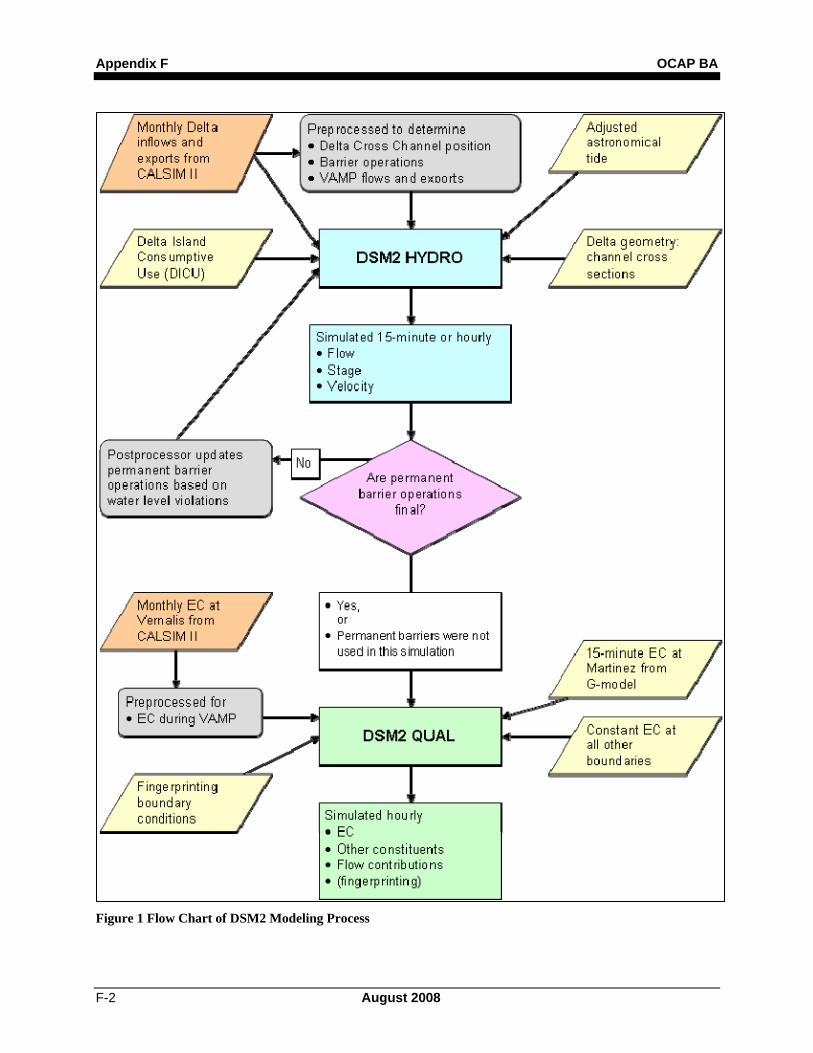
Appendix F Sacramento-San Joaquin Delta Hydrodynamic and Water Quality Model (DSM2 Model) This appendix presents an overview of the Delta Simulation Model Version 2 (DSM2). The major sections describe the DSM2 model development history, modules, modeling methods, calibration, validation, inputs and assumptions for the OCAP simulations. Due to file size limitations, the figures in this appendix are provided as an attachment electronically. 1. DSM2 Model Overview DSM2 is a one-dimensional mathematical model for dynamic simulation of tidal hydraulics, water quality, and particle tracking in a network of riverine or estuarine channels. DSM2 can calculate stages, flows, velocities, transport of individual particles, and mass transport processes for conservative and non-conservative constituents, including salts, water temperature, dissolved oxygen (DO), and dissolved organic carbon (DOC). Figure 1 shows the flow chart of DSM2 modeling process. The DWR Delta Modeling section 15th annual report (June 1994) described the initial development of DSM2, which includes the USGS four-point flow model (FOURPT) and the USGS branch Lagrangian transport model (BLTM). The 16th annual report (June 1995) described DSM2 in more detail. Calibration and verification of DSM2 has continued and resulted in many modifications and improvements that have increased the model accuracy. DSM2 formulations, as well as the procedures for specifying input data and displaying results, have been modified and improved in many important ways during the 10 years since it was first developed. The existing version of DSM2 is the result of many individuals’ efforts and has been improved by the application to many DWR and CALFED Bay-Delta Program (CALFED) projects. The application of DSM2 to the OCAP studies is described in the following sections of this chapter. DSM2 is the best available tool for Delta tidal hydraulic, water quality and particle tracking modeling and is appropriate for describing the existing and future conditions in the Delta, as well as performing simulations for the assessment of environmental impacts (i.e., incremental changes caused by facilities and operations).

Appendix F OCAP BA

F-2 August 2008

Figure 1 Flow Chart of DSM2 Modeling Process

OCAP BA Appendix F

August 2008 F-3

2. DSM2 Modules DSM2 includes three Modules: HYDRO (hydrodynamics), QUAL (water quality), and PTM (particle tracking). The three modules are briefly described below:

• The HYDRO module is a one-dimensional, implicit, unsteady, open channel flow model that DWR developed from FOURPT, a four-point finite-difference model originally developed by the USGS in Reston, Virginia. DWR adapted the model to the Delta by revising the input-output system, including open water elements, and incorporating water project facilities, such as gates, barriers, and the CCF.

• The QUAL module is a one-dimensional water quality transport model that DWR adapted from the Branched Lagrangian Transport Model originally developed by the USGS in Reston, Virginia. DWR added many enhancements to the QUAL module, such as open water areas and gates. A Lagrangian feature in the formulation eliminates the numerical dispersion that is inherently in other segmented formulations, although the tidal dispersion coefficients must still be specified.

• The PTM module simulates the transport and fate of individual particles traveling throughout the Delta. The model uses velocity, flow, and stage output from the HYDRO module to monitor the location of each individual particle using assumed vertical and lateral velocity profiles and specified random movement to simulate mixing.

2.1. HYDRO Module The HYDRO module is a tool to study the complex tidal hydraulic system found in the Delta. This module is adapted from FOURPT, a finite-difference, one-dimensional, unsteady, open channel hydrodynamic model (Delong et al. 1993). Some of the main characteristics of the HYDRO module are described below:

• The method of solving the hydrodynamic equations is fully implicit and unconditionally stable. Larger time steps can be used compared to an explicit model, which requires smaller time steps for numerical stability.

• The model is capable of handling trapezoidal and irregular shaped channels. • The model includes the baroclinic momentum equation term (i.e., density-driven flow) in

the mathematical formulation. If the density of the water is allowed to vary, its effect can be included in the analysis with the g dp / dx term in the momentum equation. The baroclinic effects on the 1-D tidal hydraulics are very small, however.

• FOURPT is capable of enforcing continuity both at a junction and within a channel because of its implicit nature.

• The HYDRO module solves the momentum and continuity equations. These differential equations are solved using a finite difference scheme requiring four points of computation, thus the name FOURPT. The equations are integrated in time and space, which leads to a solution of a set of nonlinear equations, with the incremental changes in stage and flow at the computational points as the unknowns.

Appendix F OCAP BA

F-4 August 2008

Open Water Areas A few open water areas, including the CCF, are modeled in the DSM2 grid. These areas are bodies of water that are too big to be modeled as channels. Open water areas are treated like tanks, with a known surface area and bottom elevation. An open water area can be connected to one or more channels. The flow interaction between the open water area and each of the connecting channels is determined using the general orifice formula: q = CA where q is the flow from the open water area to the channel, C is the flow coefficient, A is the flow area, and ∆h is the head difference between the open water area and the channel. The variable gate opening of the CCF intake gates cannot be simulated, but the overall flows into the CCF are reasonably represented with this orifice equation. Hydraulic Gates The flow through hydraulic gates is also calculated using the orifice flow equation. Gates can be placed either at the upstream or downstream end of a channel. Two values of gate flow coefficients are assigned for every gate, one for seaward flow and the other for landward flow. For a one-way gate, the flow coefficient assigned to the obstructed direction is set to zero. For a complete barrier, the gate flow coefficients for both directions are set to zero. FOURPT enforces an “equal stage” boundary condition for all the channels connected to a junction with no gates. Once the location of a gate is defined, the boundary condition for the gated channel is modified from “equal stage” to “known flow,” with the calculated flow. Using the current version of DSM2, the gates are allowed to open and close multiple times during a single model run using a predetermined operation rules. 2.2. QUAL Module The QUAL module is a one-dimensional transport model that predicts the fate of various water quality constituents, such as salinity (EC), temperature, DO, and DOC. As water moves tidally within the Delta channels, the constituents tend to disperse in the longitudinal direction. Other processes include growth and decay, which may be caused by interactions among various constituents. Simulation of these processes is accomplished with the conservation of mass equation, using the tidal flows and volumes calculated by the HYDRO module. Two main techniques are available for solving this equation:

• Eulerian (fixed coordinate system)—With this approach, the processes are easier to conceptualize as inflows and outflow from a “box.” As it turns out, however, the computations are fairly difficult, and the results can be inaccurate and unstable. A byproduct of this approach is an error term called the numerical dispersion, which can be significant, especially in areas with a sharp gradient in the constituent concentrations.

• Lagrangian (moving coordinate system)—With this approach, each river segment is modeled as several fixed volume water parcels, each moving with the same speed as the river flow. Using this approach, the complex convective terms are eliminated. At the

OCAP BA Appendix F

August 2008 F-5

junctions, parcels from neighboring channels are blended to create new parcels. The dispersive term is simulated as exchange between each neighboring parcel. The growth/decay terms are computed within each individual parcel. Tracking of each individual parcel requires massive amounts of bookkeeping.

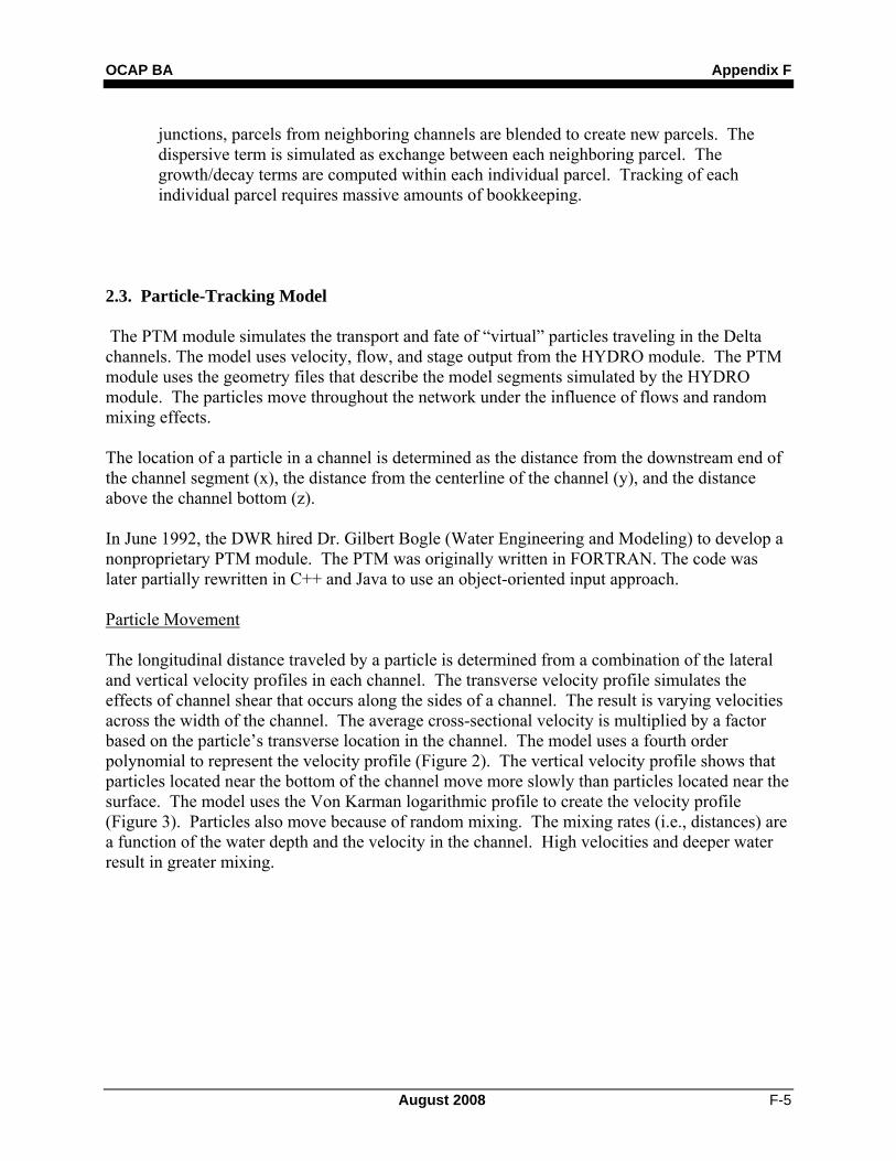
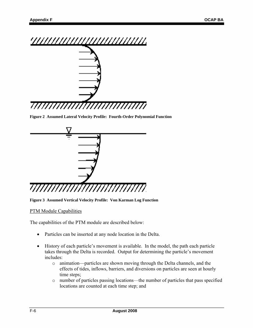
2.3. Particle-Tracking Model The PTM module simulates the transport and fate of “virtual” particles traveling in the Delta channels. The model uses velocity, flow, and stage output from the HYDRO module. The PTM module uses the geometry files that describe the model segments simulated by the HYDRO module. The particles move throughout the network under the influence of flows and random mixing effects. The location of a particle in a channel is determined as the distance from the downstream end of the channel segment (x), the distance from the centerline of the channel (y), and the distance above the channel bottom (z). In June 1992, the DWR hired Dr. Gilbert Bogle (Water Engineering and Modeling) to develop a nonproprietary PTM module. The PTM was originally written in FORTRAN. The code was later partially rewritten in C++ and Java to use an object-oriented input approach. Particle Movement The longitudinal distance traveled by a particle is determined from a combination of the lateral and vertical velocity profiles in each channel. The transverse velocity profile simulates the effects of channel shear that occurs along the sides of a channel. The result is varying velocities across the width of the channel. The average cross-sectional velocity is multiplied by a factor based on the particle’s transverse location in the channel. The model uses a fourth order polynomial to represent the velocity profile (Figure 2). The vertical velocity profile shows that particles located near the bottom of the channel move more slowly than particles located near the surface. The model uses the Von Karman logarithmic profile to create the velocity profile (Figure 3). Particles also move because of random mixing. The mixing rates (i.e., distances) are a function of the water depth and the velocity in the channel. High velocities and deeper water result in greater mixing.

Appendix F OCAP BA

F-6 August 2008

Figure 2 Assumed Lateral Velocity Profile: Fourth-Order Polynomial Function

Figure 3 Assumed Vertical Velocity Profile: Von Karman Log Function PTM Module Capabilities The capabilities of the PTM module are described below:

• Particles can be inserted at any node location in the Delta. • History of each particle’s movement is available. In the model, the path each particle

takes through the Delta is recorded. Output for determining the particle’s movement includes:

o animation—particles are shown moving through the Delta channels, and the effects of tides, inflows, barriers, and diversions on particles are seen at hourly time steps;

o number of particles passing locations—the number of particles that pass specified locations are counted at each time step; and

OCAP BA Appendix F

August 2008 F-7

o number of particles within a specified group of channels and reservoirs— the number of particles left in the channels at the end of the time step.

• Each particle has a unique identity, and characteristics can change over time. Because each particle is individually tracked, characteristics (behavior) can be assigned to the particle. Examples of characteristics are additional velocities that represent behavior (self-induced velocities) and the state of the particle, such as age.

• Particles can have a settling (or buoyancy) velocity. Therefore, if particles are heavy and tend to sink toward the bottom, they will move more slowly than if they were neutrally buoyant or floating. As a result, the travel time of heavy particles through the channels will be longer.

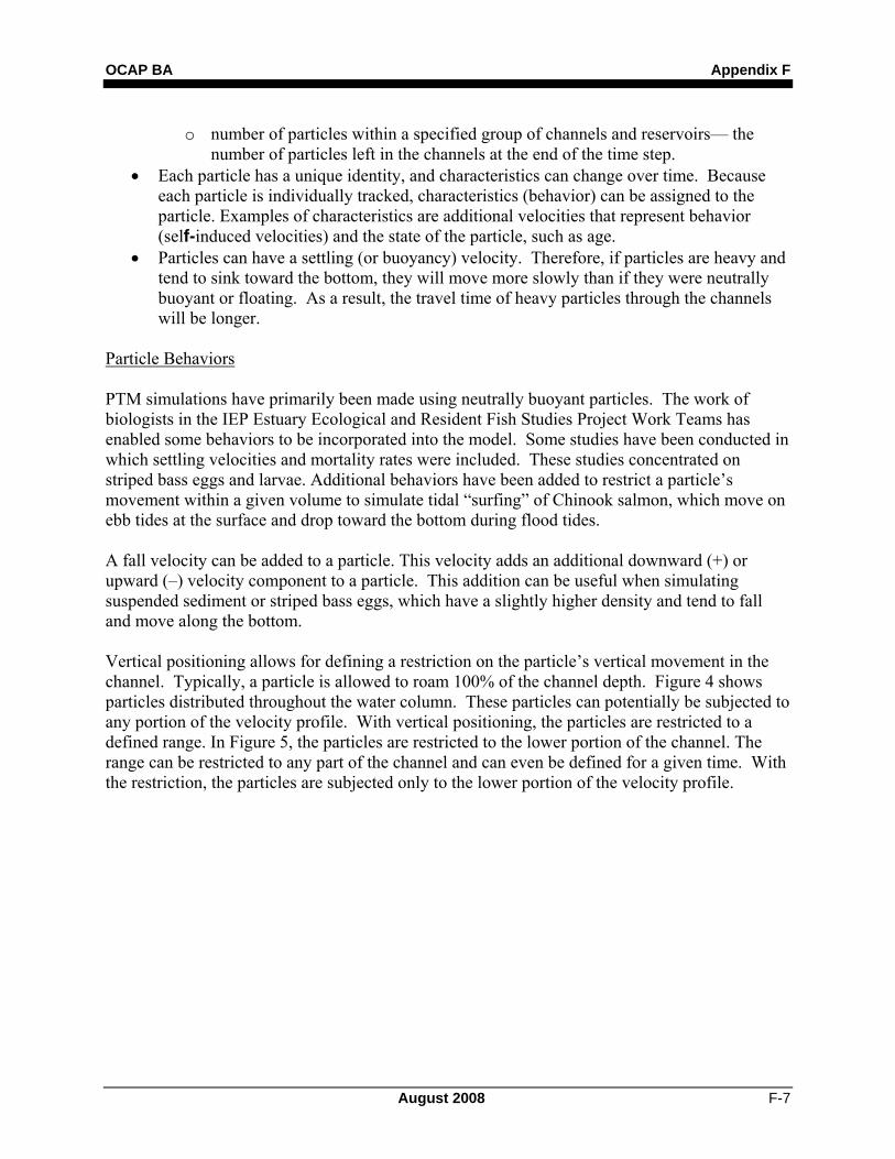
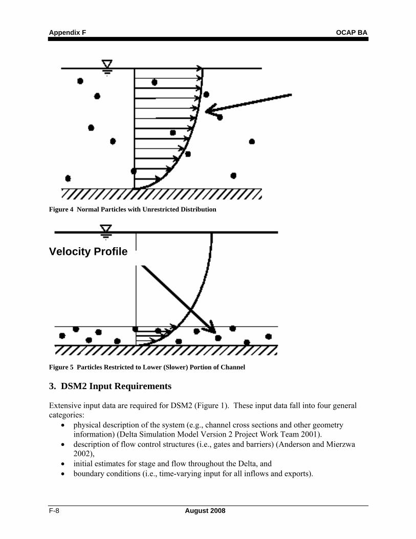
Particle Behaviors PTM simulations have primarily been made using neutrally buoyant particles. The work of biologists in the IEP Estuary Ecological and Resident Fish Studies Project Work Teams has enabled some behaviors to be incorporated into the model. Some studies have been conducted in which settling velocities and mortality rates were included. These studies concentrated on striped bass eggs and larvae. Additional behaviors have been added to restrict a particle’s movement within a given volume to simulate tidal “surfing” of Chinook salmon, which move on ebb tides at the surface and drop toward the bottom during flood tides. A fall velocity can be added to a particle. This velocity adds an additional downward (+) or upward (–) velocity component to a particle. This addition can be useful when simulating suspended sediment or striped bass eggs, which have a slightly higher density and tend to fall and move along the bottom. Vertical positioning allows for defining a restriction on the particle’s vertical movement in the channel. Typically, a particle is allowed to roam 100% of the channel depth. Figure 4 shows particles distributed throughout the water column. These particles can potentially be subjected to any portion of the velocity profile. With vertical positioning, the particles are restricted to a defined range. In Figure 5, the particles are restricted to the lower portion of the channel. The range can be restricted to any part of the channel and can even be defined for a given time. With the restriction, the particles are subjected only to the lower portion of the velocity profile.

Appendix F OCAP BA

F-8 August 2008

Figure 4 Normal Particles with Unrestricted Distribution

Figure 5 Particles Restricted to Lower (Slower) Portion of Channel 3. DSM2 Input Requirements Extensive input data are required for DSM2 (Figure 1). These input data fall into four general categories:

• physical description of the system (e.g., channel cross sections and other geometry information) (Delta Simulation Model Version 2 Project Work Team 2001).

• description of flow control structures (i.e., gates and barriers) (Anderson and Mierzwa 2002),

• initial estimates for stage and flow throughout the Delta, and • boundary conditions (i.e., time-varying input for all inflows and exports).

Velocity Profile

OCAP BA Appendix F

August 2008 F-9

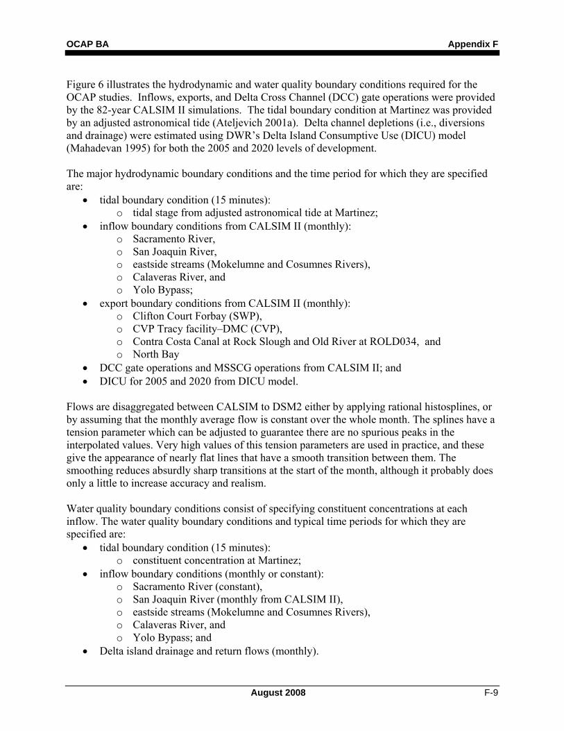
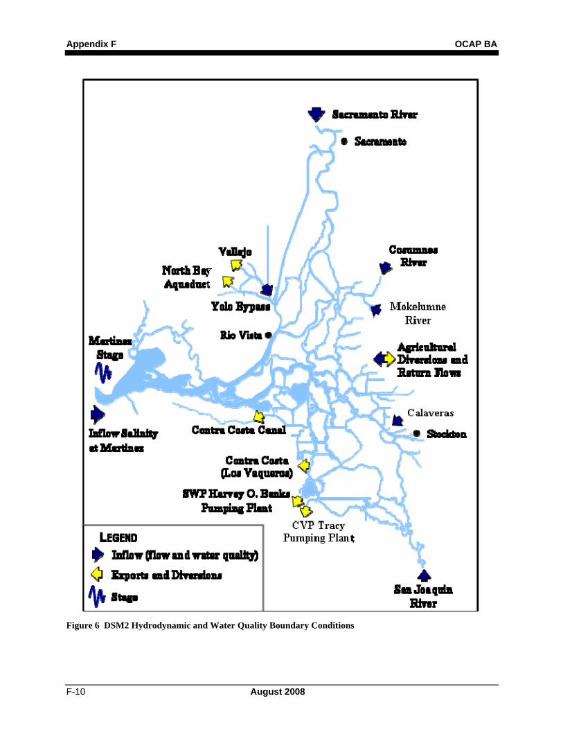
Figure 6 illustrates the hydrodynamic and water quality boundary conditions required for the OCAP studies. Inflows, exports, and Delta Cross Channel (DCC) gate operations were provided by the 82-year CALSIM II simulations. The tidal boundary condition at Martinez was provided by an adjusted astronomical tide (Ateljevich 2001a). Delta channel depletions (i.e., diversions and drainage) were estimated using DWR’s Delta Island Consumptive Use (DICU) model (Mahadevan 1995) for both the 2005 and 2020 levels of development. The major hydrodynamic boundary conditions and the time period for which they are specified are:

• tidal boundary condition (15 minutes): o tidal stage from adjusted astronomical tide at Martinez;

• inflow boundary conditions from CALSIM II (monthly): o Sacramento River, o San Joaquin River, o eastside streams (Mokelumne and Cosumnes Rivers), o Calaveras River, and o Yolo Bypass;

• export boundary conditions from CALSIM II (monthly): o Clifton Court Forbay (SWP), o CVP Tracy facility–DMC (CVP), o Contra Costa Canal at Rock Slough and Old River at ROLD034, and o North Bay

• DCC gate operations and MSSCG operations from CALSIM II; and • DICU for 2005 and 2020 from DICU model.

Flows are disaggregated between CALSIM to DSM2 either by applying rational histosplines, or by assuming that the monthly average flow is constant over the whole month. The splines have a tension parameter which can be adjusted to guarantee there are no spurious peaks in the interpolated values. Very high values of this tension parameters are used in practice, and these give the appearance of nearly flat lines that have a smooth transition between them. The smoothing reduces absurdly sharp transitions at the start of the month, although it probably does only a little to increase accuracy and realism. Water quality boundary conditions consist of specifying constituent concentrations at each inflow. The water quality boundary conditions and typical time periods for which they are specified are:

• tidal boundary condition (15 minutes): o constituent concentration at Martinez;

• inflow boundary conditions (monthly or constant): o Sacramento River (constant), o San Joaquin River (monthly from CALSIM II), o eastside streams (Mokelumne and Cosumnes Rivers), o Calaveras River, and o Yolo Bypass; and

• Delta island drainage and return flows (monthly).

Appendix F OCAP BA

F-10 August 2008

Figure 6 DSM2 Hydrodynamic and Water Quality Boundary Conditions

OCAP BA Appendix F

August 2008 F-11

4. DSM2 Calibration and Validation 4.1. DSM2 Calibration The DSM2-modeled tidal hydraulic and salinity (EC) results were initially calibrated in 1997 by the DWR Delta modeling staff. The IEP PWT for DSM2 calibration and validation provided additional calibration during 1999. The recent network of USGS tidal flow meters as well as these more extensive geometry measurements provided the motivation for the PWT calibration and validation efforts for the newest version of the Delta tidal hydraulic and water quality model, DSM2. The HYDRO module was calibrated using data from four different time periods:

• May 1988, April 1997, • April 1998, and • September and October 1998.

For the HYDRO module, the Manning’s roughness coefficient n was chosen as the calibration parameter. With each subsequent run, these coefficient values were modified to try to achieve a better match. Phase and tidal amplitude error indexes were introduced to quantify the exactness of fit for tidal stage. The magnitude of the error indexes was calculated for each period separately, and these values were added to the calibration figures. Showing the error indexes directly on the figures made it easier to improve the calibrated match. Fifty-six iterations were run. Overall, model predictions for the final iteration of the calibration are noticeably closer to the field data than the original 1997 calibration. The QUAL module was calibrated in one continuous interval because QUAL results can be affected by the initial conditions (salinity) for several months. QUAL was calibrated using EC data because EC data are plentiful, and EC is assumed to behave like a conservative substance. The most suitable periods for calibration of salinity are dry periods during which saline Bay water enters the Delta. The IEP Project Work Team (PWT) selected the 3-year period from October 1991 to September 1994 for calibration. Dispersion coefficients were used as the calibration parameter. After 16 iterations, the PWT decided that the EC calibration was complete. Overall, QUAL results and the actual EC data agree quite well. Salt intrusion into the western Delta was simulated fairly well. However, in the San Joaquin River between Antioch and Jersey Point and continuing up Old River to Bacon Island, the model over-predicts the salt intrusion. 4.2. Validation of DSM2-Simulated Tidal Stage and Flow Delta tidal hydraulic simulations of stage and flow (velocity) and salinity (EC) with DSM2 are important for many proposed projects, such as the DWR South Delta Improvement Plan (SDIP), wastewater treatment plant discharge, fish protection efforts such as the Vernalis Adaptive Management Plan (VAMP), and flood control and levee maintenance efforts. The accurate simulation of project effects depends on reliable model calibration and application. This section of the appendix demonstrates that DSM2 has been accurately calibrated by showing the

Appendix F OCAP BA

F-12 August 2008

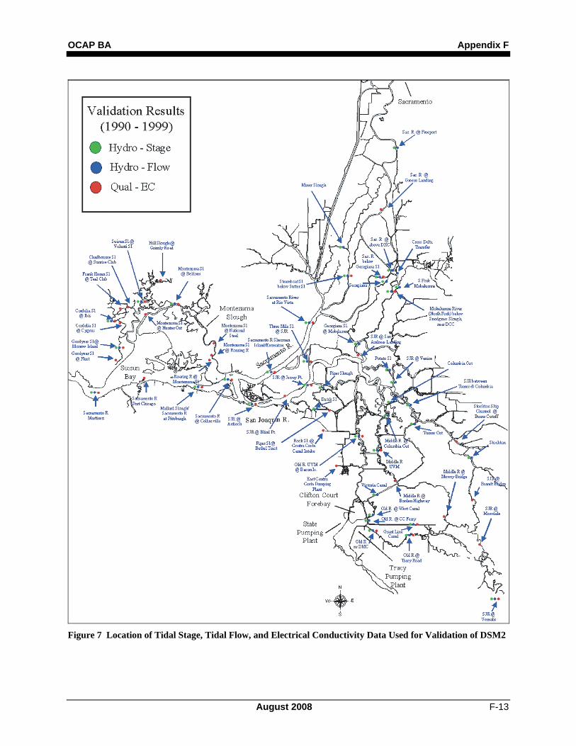
comparison of measurements and simulations of tidal hydraulic stage and flow and salinity conditions from several recent years. The OCAP simulations are therefore considered to be a very reliable basis for impact evaluations. A 6-year historical simulation of the January 1994–September 1999 period was used for a validation period. The historical tides at Martinez were used along with the daily average inflows and export pumping to produce this 6-year continuous simulation. The previous results (1997 calibration) are shown together with the most recent calibration results and the field data. The results of this interagency calibration effort are documented in a series of graphs on the website at: http://modeling.water.ca.gov/delta/studies/validation2000. The draft calibration and validation report is available at: http://www.iep.ca.gov/dsm2pwt/dsm2pwt.html A considerable effort has been made to improve the channel geometry specified for the DSM2 grid. Channel geometry is perhaps the major factor influencing the tidal hydraulics in the Delta. Modern methods of boat-mounted depth sounder connected with a GPS for location have been used to collect more accurate bathymetry data in several portions of the Delta by DWR Central District staff. All the bathymetry data are contained in the geometry database and user-interface called the “Cross Section Development Program.” More than 50 separate model runs were performed to adjust the flow friction coefficient (Manning’s roughness coefficient n) values to match the stage and velocity and phase lag throughout the Delta. Salinity (EC) was calibrated by adjusting the salinity dispersion coefficient. The results of this extensive calibration effort are demonstrated in the selected validation results shown in this section. The validation simulation used historical daily inflows and export pumping with historical tidal stage at Martinez to simulate the January 1994–September 1999 period, using the calibrated geometry and model coefficients. This period includes a wide range of flow and export pumping, with temporary barriers installed during the spring and summer months. The tidal stage comparisons for the higher flow periods are reviewed below to illustrate the accuracy of the DSM2 simulations during major flood events. Several major floods, including the January 1997 events, are simulated in these historical DSM2 results. Tidal stage comparisons in the lower flow periods illustrate the ability of DSM2 to match the normal tidal fluctuations in the Delta. Figure 7 shows the Delta stations with field data (tidal stage, tidal flow, or EC) that were compared during the DSM2 validation efforts. Two periods are selected to illustrate the validation of DSM2 for selected stations throughout the Delta. The daily average tidal stages and flows are shown for a 3-year period of January 1997–September 1999. The 15-minute tidal stage and flow results are compared to measured stage and flow variations for the 2-week period of February 17–March 2, 1996.

OCAP BA Appendix F

August 2008 F-13

Figure 7 Location of Tidal Stage, Tidal Flow, and Electrical Conductivity Data Used for Validation of DSM2

Appendix F OCAP BA

F-14 August 2008

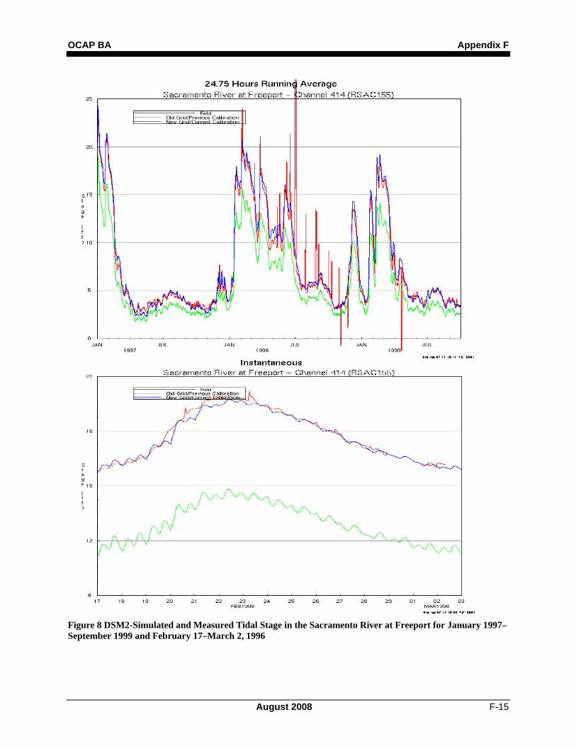
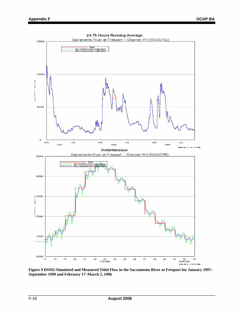
Validation at Sacramento River Locations For the Sacramento River at Freeport, Figure 8 shows the simulated and measured tidal stage and Figure 9 shows the simulated and measured tidal flows. The initial calibration (green) did not match the tidal stage at higher flows. The tidal stage was about 4 feet too low when the flow was greater than 50,000 cfs, but was about 1 foot too low during lower flows of about 10,000 cfs. The revised calibration provides a very good match with the high tidal stages resulting from large flows in the Sacramento River. There is a USGS tidal flow meter at Freeport, but the daily average flows that are used as input at the upstream model boundary near downtown Sacramento are shown in the flow graph.

OCAP BA Appendix F

August 2008 F-15

Figure 8 DSM2-Simulated and Measured Tidal Stage in the Sacramento River at Freeport for January 1997–September 1999 and February 17–March 2, 1996

Appendix F OCAP BA

F-16 August 2008

Figure 9 DSM2-Simulated and Measured Tidal Flow in the Sacramento River at Freeport for January 1997–September 1999 and February 17–March 2, 1996

OCAP BA Appendix F

August 2008 F-17

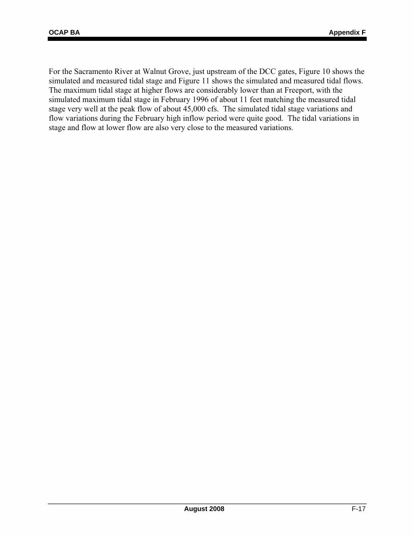
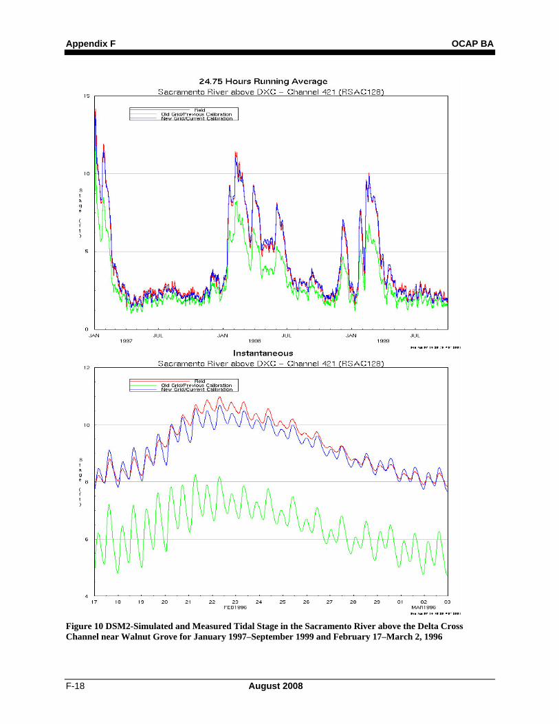
For the Sacramento River at Walnut Grove, just upstream of the DCC gates, Figure 10 shows the simulated and measured tidal stage and Figure 11 shows the simulated and measured tidal flows. The maximum tidal stage at higher flows are considerably lower than at Freeport, with the simulated maximum tidal stage in February 1996 of about 11 feet matching the measured tidal stage very well at the peak flow of about 45,000 cfs. The simulated tidal stage variations and flow variations during the February high inflow period were quite good. The tidal variations in stage and flow at lower flow are also very close to the measured variations.

Appendix F OCAP BA

F-18 August 2008

Figure 10 DSM2-Simulated and Measured Tidal Stage in the Sacramento River above the Delta Cross Channel near Walnut Grove for January 1997–September 1999 and February 17–March 2, 1996

OCAP BA Appendix F

August 2008 F-19

Figure 11 DSM2-Simulated and Measured Tidal Flow in the Sacramento River above the Delta Cross Channel near Walnut Grove for January 1997–September 1999 and February 17–March 2, 1996 (Delta Cross Channel Closed)

Appendix F OCAP BA

F-20 August 2008

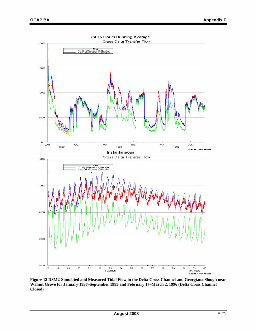
For the DCC and Georgiana Slough, Figure 12 shows both the daily average combined flows for the 1997–1999 period and the tidal flows simulated in Georgiana Slough during the February 1996 high-flow event, when the DCC was closed because the Freeport flows were above 25,000 cfs. The new calibration appears to give an accurate flow split for periods with the DCC gates either open or closed (February–June and during high flows). The tidal variation in Georgiana Slough stage and flow during the February 1996 high-flow event (when DCC was closed) are quite close to the measured data.

OCAP BA Appendix F

August 2008 F-21

Figure 12 DSM2-Simulated and Measured Tidal Flow in the Delta Cross Channel and Georgiana Slough near Walnut Grove for January 1997–September 1999 and February 17–March 2, 1996 (Delta Cross Channel Closed)

Appendix F OCAP BA

F-22 August 2008

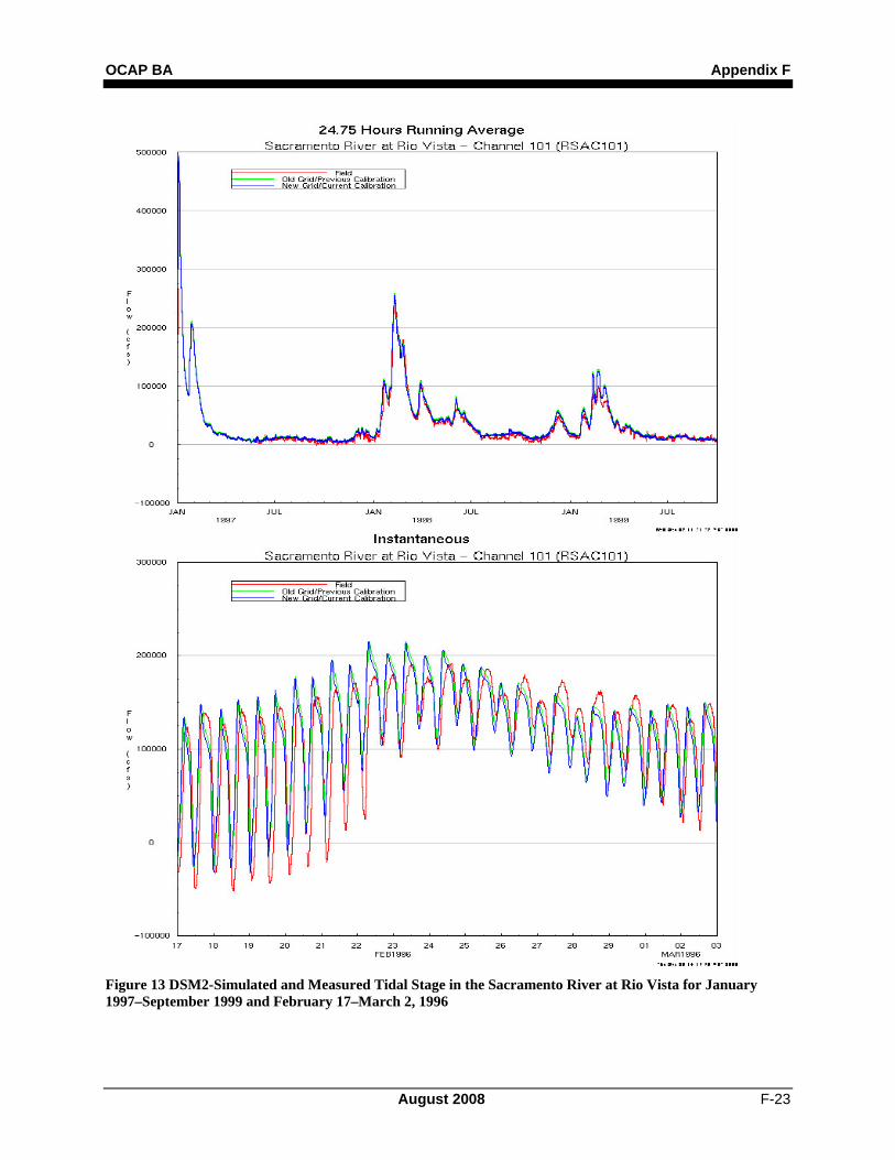
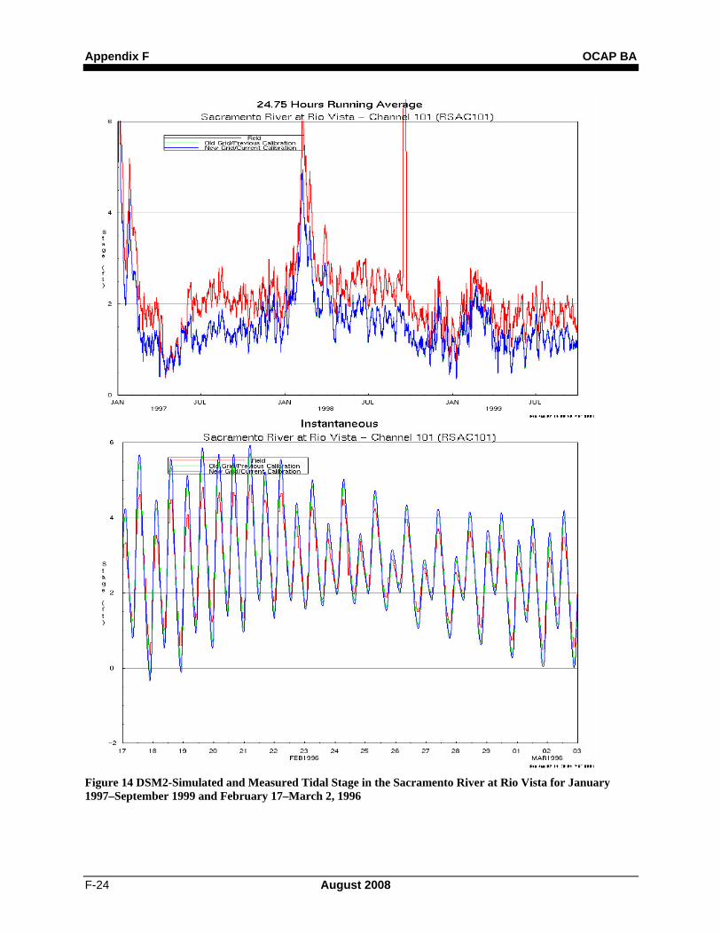
For the Sacramento River at Rio Vista, Figure 13 shows the simulated and measured tidal stage and Figure 14 shows the simulated and measured tidal flows. Flows at Rio Vista can be quite high because the Yolo Bypass joins the Sacramento River channel just upstream. The simulated daily average tidal stages at higher flows are only 4–6 feet NGVD. The tidal stage variation during February 1996 high-flow event when the flows were between 50,000 cfs and 150,000 cfs were well matched, with a 4-foot tidal variation (i.e., high tide minus low tide) during moderate flows of 50,000 cfs, and a 2.5-foot tidal stage variation even during the peak flow of 150,000 cfs. This indicates that the tidal variations dominate the tidal flows at Rio Vista, even when the inflows are 150,000 cfs. The simulated tidal variation is about 0.5 foot greater than measured.

OCAP BA Appendix F

August 2008 F-23

Figure 13 DSM2-Simulated and Measured Tidal Stage in the Sacramento River at Rio Vista for January 1997–September 1999 and February 17–March 2, 1996

Appendix F OCAP BA

F-24 August 2008

Figure 14 DSM2-Simulated and Measured Tidal Stage in the Sacramento River at Rio Vista for January 1997–September 1999 and February 17–March 2, 1996

OCAP BA Appendix F

August 2008 F-25

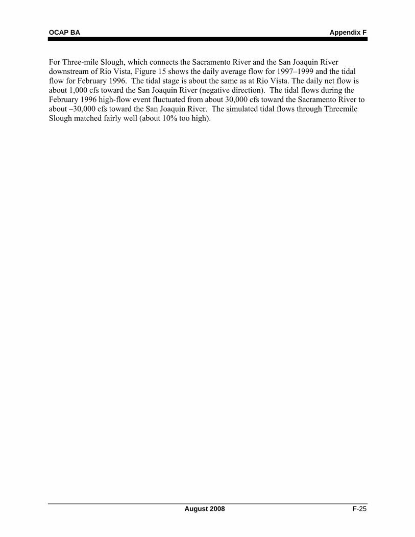
For Three-mile Slough, which connects the Sacramento River and the San Joaquin River downstream of Rio Vista, Figure 15 shows the daily average flow for 1997–1999 and the tidal flow for February 1996. The tidal stage is about the same as at Rio Vista. The daily net flow is about 1,000 cfs toward the San Joaquin River (negative direction). The tidal flows during the February 1996 high-flow event fluctuated from about 30,000 cfs toward the Sacramento River to about –30,000 cfs toward the San Joaquin River. The simulated tidal flows through Threemile Slough matched fairly well (about 10% too high).

Appendix F OCAP BA

F-26 August 2008

Figure 15 DSM2-Simulated and Measured Tidal Flow in Threemile Slough for 1997–1999 and February 17–March 2, 1996 (Positive Flow toward Sacramento River)

OCAP BA Appendix F

August 2008 F-27

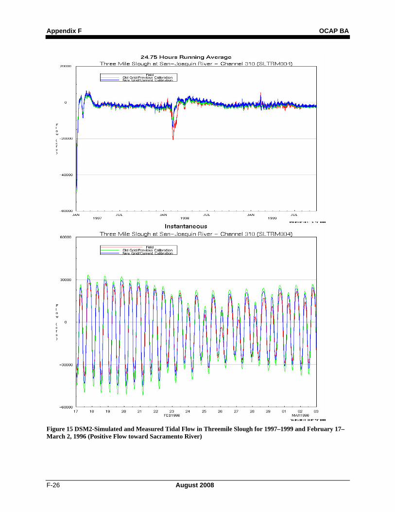
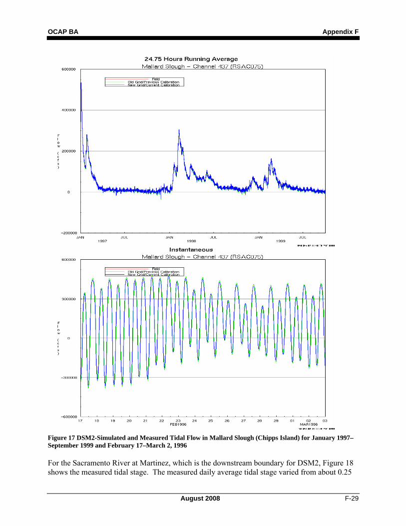
For the Sacramento River at Mallard Slough (across from Chipps Island), Figure 16 shows the simulated and measured tidal stage and Figure 17 shows the simulated and measured tidal flows. The simulated daily average tidal stages at higher flows are only 3 feet NGVD. The tidal stage variation during February 1996 when the Delta outflows were between 50,000 and 150,000 cfs were well matched, with a 4.5-foot tidal variation (i.e., high tide minus low tide) during moderate flows of 50,000 cfs, and a 3.5-foot tidal stage variation even during the peak flow of 150,000 cfs. The simulated tidal variation is about 0.5 foot greater than measured during the beginning of the event and is almost exactly the same during the period of highest flows.

Appendix F OCAP BA

F-28 August 2008

Figure 16 DSM2-Simulated and Measured Tidal Stage in Mallard Slough (Chipps Island) for January 1997–September 1999 and February 17–March 2, 1996

OCAP BA Appendix F

August 2008 F-29

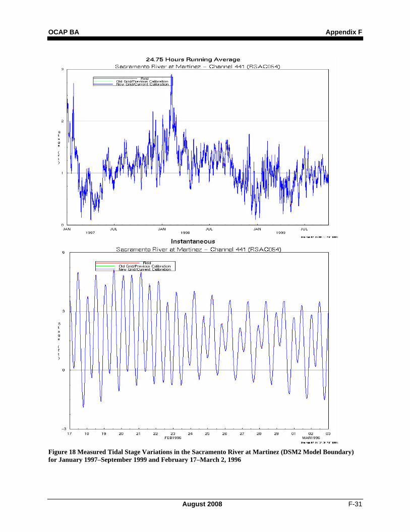
Figure 17 DSM2-Simulated and Measured Tidal Flow in Mallard Slough (Chipps Island) for January 1997–September 1999 and February 17–March 2, 1996 For the Sacramento River at Martinez, which is the downstream boundary for DSM2, Figure 18 shows the measured tidal stage. The measured daily average tidal stage varied from about 0.25

Appendix F OCAP BA

F-30 August 2008

to 2.75 feet NGVD during the high outflow periods, and averages about 1 feet NGVD. The tidal stage variation at Martinez can be quite large (i.e., more than 6 feet), and was reduced to a variation of about 4 feet during the peak outflow of 150,000 cfs during the February 1996 high-flow event. DSM2 does a good job of propagating this measured tidal stage variation into the Sacramento River channel all the way to Freeport.

OCAP BA Appendix F

August 2008 F-31

Figure 18 Measured Tidal Stage Variations in the Sacramento River at Martinez (DSM2 Model Boundary) for January 1997–September 1999 and February 17–March 2, 1996

Appendix F OCAP BA

F-32 August 2008

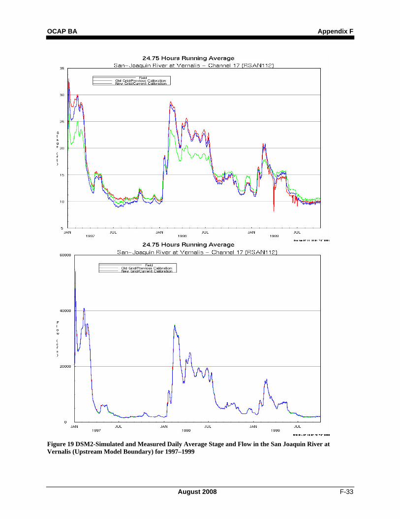
Validation at San Joaquin River Locations For the San Joaquin River at Vernalis, Figure 19 shows the DSM2-simulated and measured daily average tidal stage and flow for the 1997–1999 period. This location is the upstream boundary for DSM2 on the San Joaquin River. The calibrated tidal stage is now reasonably well matched with the data, whereas the initial calibration had a stage during high flows that was 5 feet lower than measured.

OCAP BA Appendix F

August 2008 F-33

Figure 19 DSM2-Simulated and Measured Daily Average Stage and Flow in the San Joaquin River at Vernalis (Upstream Model Boundary) for 1997–1999

Appendix F OCAP BA

F-34 August 2008

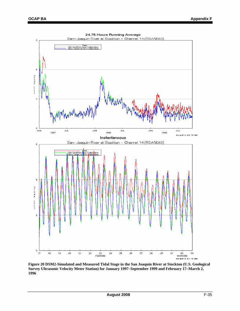
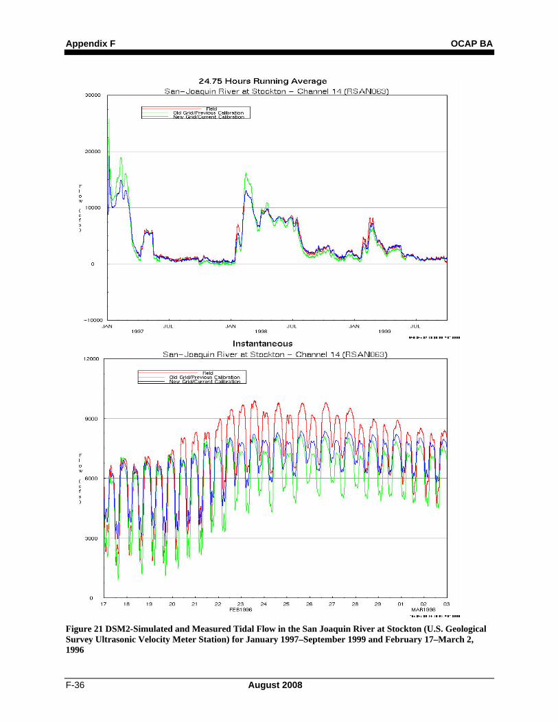
For the San Joaquin River at the Stockton UVM station, Figure 20 shows the simulated and measured tidal stage and Figure 21 shows the simulated and measured tidal flows. The simulated tidal stage is about 0.5 foot below the measured tidal stage. The simulated tidal stage variations are not well-matched with the data. The simulated minimum tidal stage is about 1 foot lower than measured during the peak flows of the February 1996 high-flow event. The simulated tidal flow is also lower than the measured tidal flow during the highest flows of the February 1996 high-flow event. The simulated tidal flows matched better during the beginning of the February 1996 high-flow event, but the simulated minimum tidal flows were too high (i.e., simulated tidal flow variation is too small).

OCAP BA Appendix F

August 2008 F-35

Figure 20 DSM2-Simulated and Measured Tidal Stage in the San Joaquin River at Stockton (U.S. Geological Survey Ultrasonic Velocity Meter Station) for January 1997–September 1999 and February 17–March 2, 1996

Appendix F OCAP BA

F-36 August 2008

Figure 21 DSM2-Simulated and Measured Tidal Flow in the San Joaquin River at Stockton (U.S. Geological Survey Ultrasonic Velocity Meter Station) for January 1997–September 1999 and February 17–March 2, 1996

OCAP BA Appendix F

August 2008 F-37

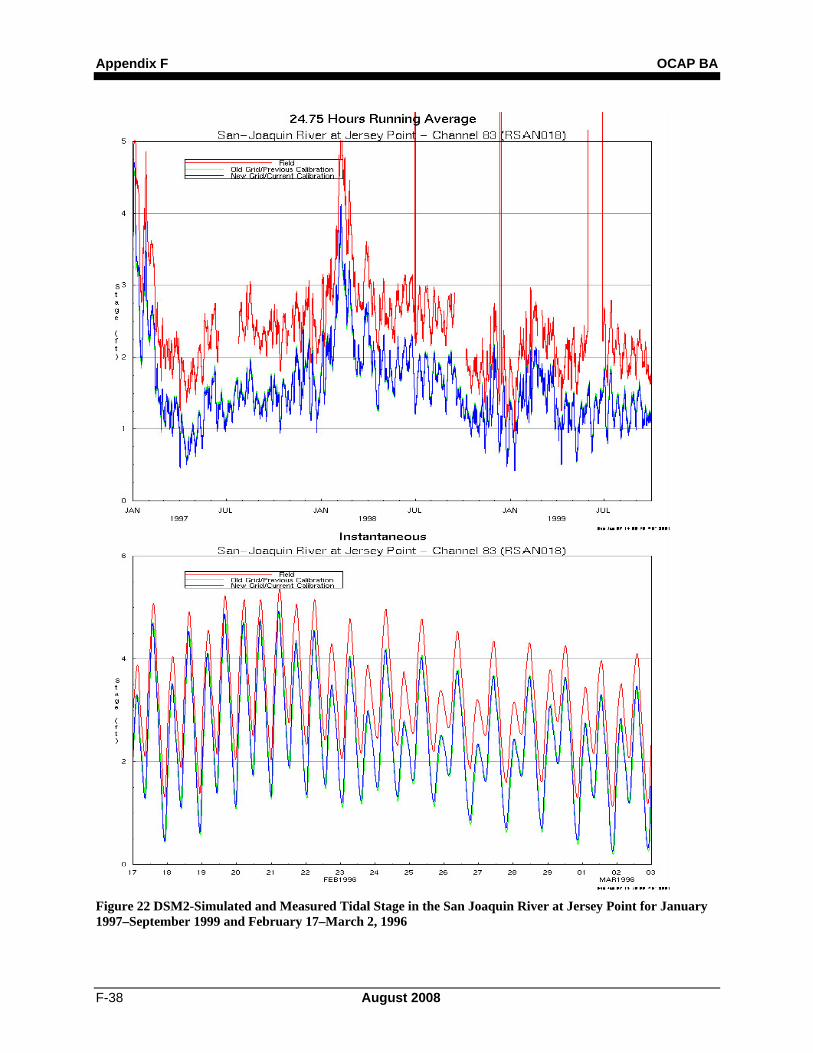
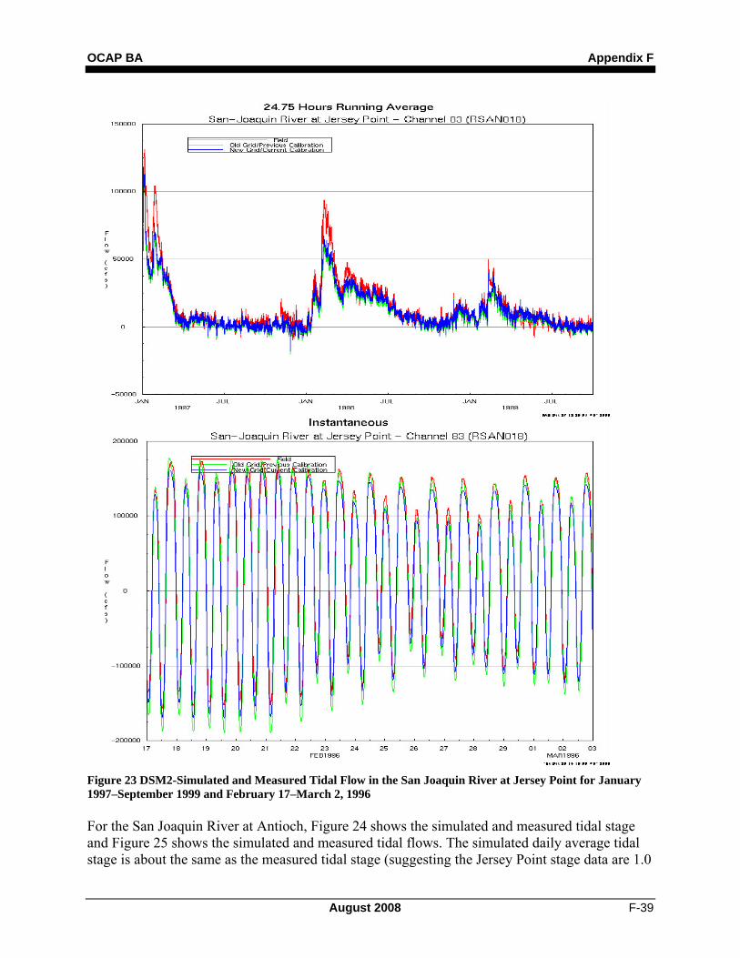
For the San Joaquin River at Jersey Island, Figure 22 shows the simulated and measured tidal stage and Figure 23 shows the simulated and measured tidal flows. The simulated tidal stage is about 1.0 foot below the measured tidal stage, although the measured tidal stage appears to be too high compared to surrounding stations (i.e., Antioch and Rio Vista). The range of net flows at Jersey Point was about 0–75,000 cfs during the 1997–1999 period, although the simulated peak net flows were only 50,000 cfs. The simulated tidal flow is close to the measured tidal flows at the Rio Vista USGS tidal flow station. The tidal flows generally range from –150,000 cfs during the moderate flows at the beginning of the February 17–March 2 period. The simulated and measured tidal flows are dampened slightly by the higher net flows at the end of this period, with flood tide maximum flows of –100,000 cfs and maximum ebb tides flows of 125,000 cfs.

Appendix F OCAP BA

F-38 August 2008

Figure 22 DSM2-Simulated and Measured Tidal Stage in the San Joaquin River at Jersey Point for January 1997–September 1999 and February 17–March 2, 1996

OCAP BA Appendix F

August 2008 F-39

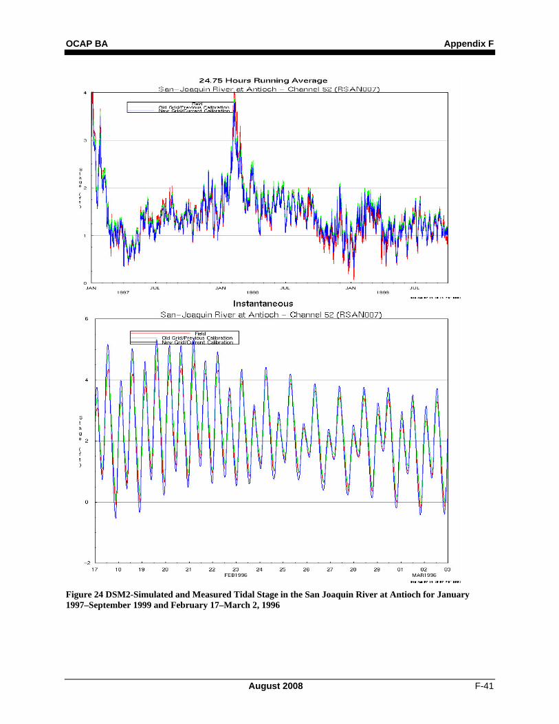
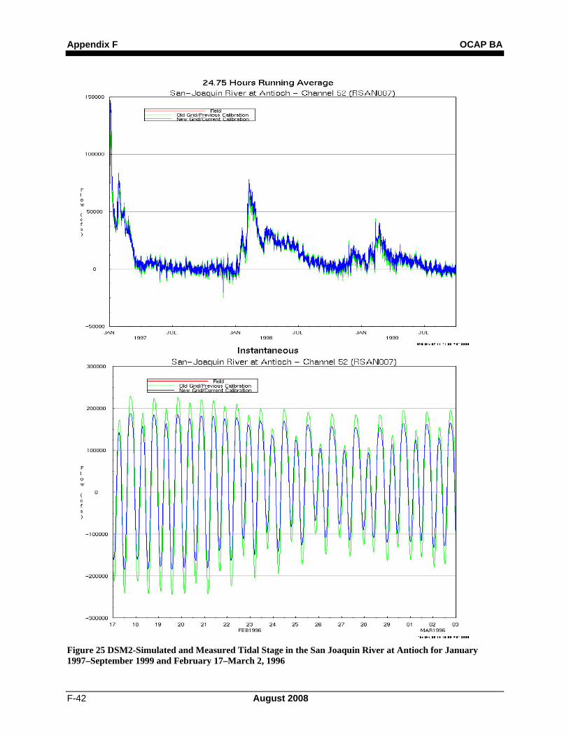
Figure 23 DSM2-Simulated and Measured Tidal Flow in the San Joaquin River at Jersey Point for January 1997–September 1999 and February 17–March 2, 1996 For the San Joaquin River at Antioch, Figure 24 shows the simulated and measured tidal stage and Figure 25 shows the simulated and measured tidal flows. The simulated daily average tidal stage is about the same as the measured tidal stage (suggesting the Jersey Point stage data are 1.0

Appendix F OCAP BA

F-40 August 2008

foot higher than actual). The tidal range during the February 1996 high-flow event was about 4 feet at the beginning and about 3 feet during the peak flow, although some of this variation is caused by the spring-neap cycle, as well as the tidal stage damping from the higher flow. The range of simulated net flows at Antioch was about 0 cfs to 50,000 cfs during the 1997–1999 period, although the measured net flows at Jersey Pint suggest the peak flows AT Antioch should be higher (same as Jersey Point net flows). The simulated tidal flows generally range from –175,000 cfs (flood) to 175,000 cfs (ebb) during the moderate flows at the beginning of the February 17-March 2 period. The simulated tidal flows are damped out a little by the higher net flows at the end of this period, with flood tide maximum flows of –100,000 cfs and maximum ebb tides flows of 150,000 cfs. The initial calibration (green line) indicated higher tidal flows than the current calibration that matched the measured Jersey Point tidal flows.

OCAP BA Appendix F

August 2008 F-41

Figure 24 DSM2-Simulated and Measured Tidal Stage in the San Joaquin River at Antioch for January 1997–September 1999 and February 17–March 2, 1996

Appendix F OCAP BA

F-42 August 2008

Figure 25 DSM2-Simulated and Measured Tidal Stage in the San Joaquin River at Antioch for January 1997–September 1999 and February 17–March 2, 1996

OCAP BA Appendix F

August 2008 F-43

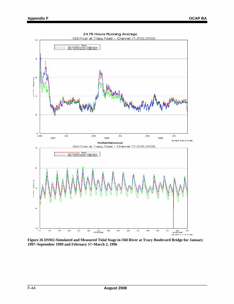
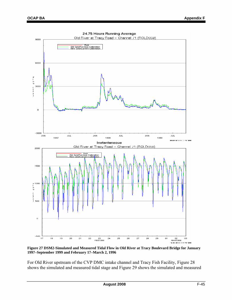
These validation results for the San Joaquin River suggest that DSM2 is very well calibrated for the San Joaquin River channel upstream to Jersey Point. There is some indication that the tidal stage and flows upstream of the Stockton are a little lower than measured. Overall, the tidal stage and flow fluctuations within the San Joaquin River, which forms the boundary for the south Delta channels, are accurately simulated by DSM2. Validation at South Delta Locations For Old River at Tracy Boulevard Bridge, Figure 26 shows the simulated and measured tidal stage and Figure 27 shows the simulated and measured tidal flows. The simulated daily average tidal stage with the new calibration now matches the measured tidal stage at higher flows of 5,000 cfs. The tidal stage variations during the February 1996 high-flow event match the measured tidal stage data reasonably well, although the simulated high tides are about 0.5 foot higher than measured. The range of simulated net flows in Old River at the Tracy Boulevard Bridge is only about 0–5,000 cfs. The simulated tidal flows (there are no measured tidal flows) are very irregular, with a pulse flood tide flow and a more steady ebb tide flow. Most of the flow entering the Old River channel from the head of Old River diversion from the San Joaquin River flows down the Grant Line Canal and does not flow past the Tracy Boulevard Bridge.

Appendix F OCAP BA

F-44 August 2008

Figure 26 DSM2-Simulated and Measured Tidal Stage in Old River at Tracy Boulevard Bridge for January 1997–September 1999 and February 17–March 2, 1996

OCAP BA Appendix F

August 2008 F-45

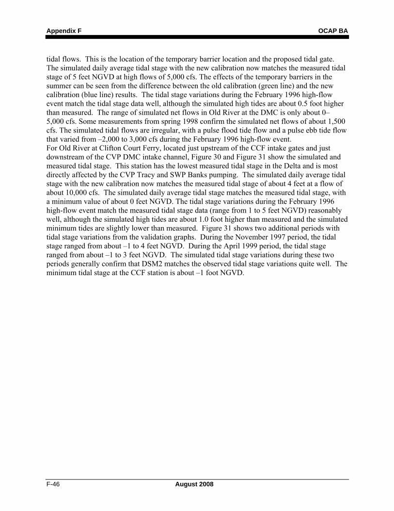
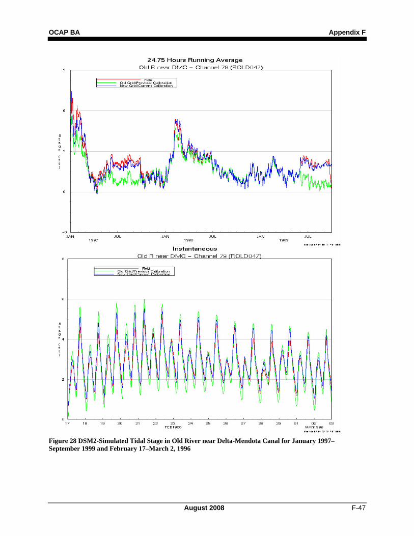
Figure 27 DSM2-Simulated and Measured Tidal Flow in Old River at Tracy Boulevard Bridge for January 1997–September 1999 and February 17–March 2, 1996 For Old River upstream of the CVP DMC intake channel and Tracy Fish Facility, Figure 28 shows the simulated and measured tidal stage and Figure 29 shows the simulated and measured

Appendix F OCAP BA

F-46 August 2008

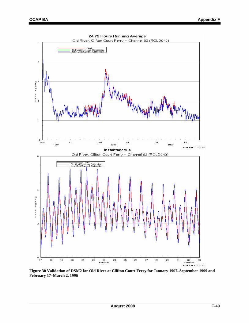
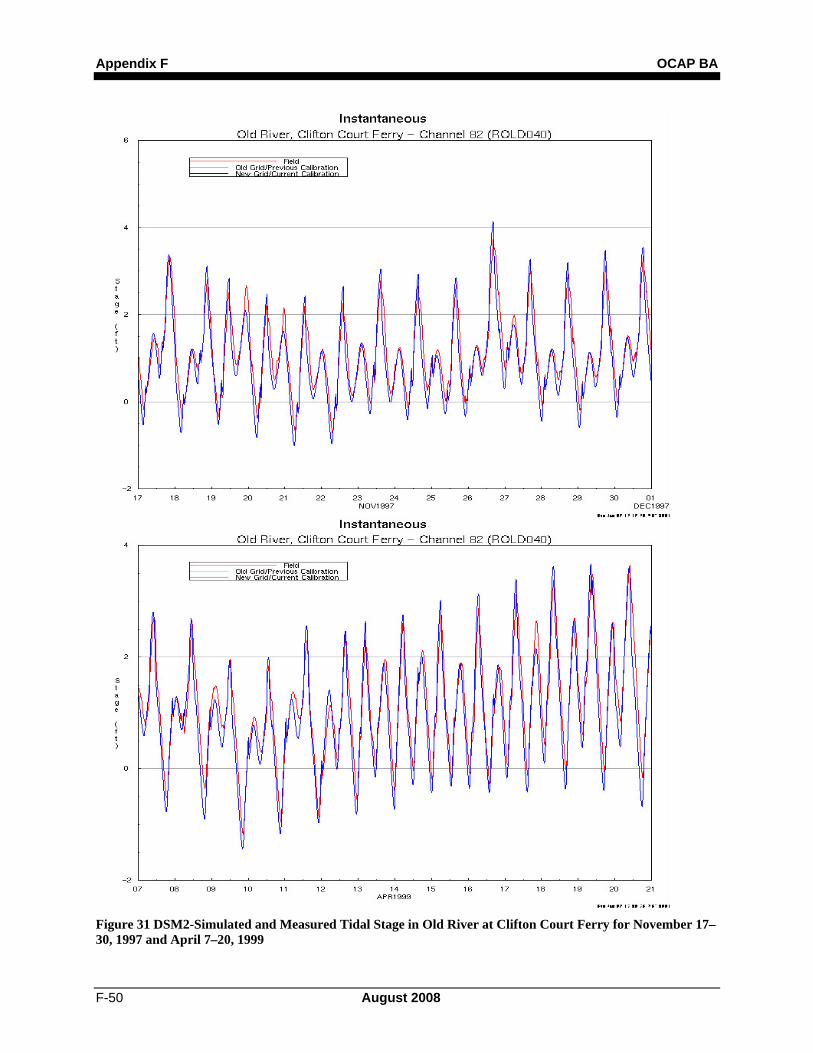
tidal flows. This is the location of the temporary barrier location and the proposed tidal gate. The simulated daily average tidal stage with the new calibration now matches the measured tidal stage of 5 feet NGVD at high flows of 5,000 cfs. The effects of the temporary barriers in the summer can be seen from the difference between the old calibration (green line) and the new calibration (blue line) results. The tidal stage variations during the February 1996 high-flow event match the tidal stage data well, although the simulated high tides are about 0.5 foot higher than measured. The range of simulated net flows in Old River at the DMC is only about 0– 5,000 cfs. Some measurements from spring 1998 confirm the simulated net flows of about 1,500 cfs. The simulated tidal flows are irregular, with a pulse flood tide flow and a pulse ebb tide flow that varied from –2,000 to 3,000 cfs during the February 1996 high-flow event. For Old River at Clifton Court Ferry, located just upstream of the CCF intake gates and just downstream of the CVP DMC intake channel, Figure 30 and Figure 31 show the simulated and measured tidal stage. This station has the lowest measured tidal stage in the Delta and is most directly affected by the CVP Tracy and SWP Banks pumping. The simulated daily average tidal stage with the new calibration now matches the measured tidal stage of about 4 feet at a flow of about 10,000 cfs. The simulated daily average tidal stage matches the measured tidal stage, with a minimum value of about 0 feet NGVD. The tidal stage variations during the February 1996 high-flow event match the measured tidal stage data (range from 1 to 5 feet NGVD) reasonably well, although the simulated high tides are about 1.0 foot higher than measured and the simulated minimum tides are slightly lower than measured. Figure 31 shows two additional periods with tidal stage variations from the validation graphs. During the November 1997 period, the tidal stage ranged from about –1 to 4 feet NGVD. During the April 1999 period, the tidal stage ranged from about –1 to 3 feet NGVD. The simulated tidal stage variations during these two periods generally confirm that DSM2 matches the observed tidal stage variations quite well. The minimum tidal stage at the CCF station is about –1 foot NGVD.

OCAP BA Appendix F

August 2008 F-47

Figure 28 DSM2-Simulated Tidal Stage in Old River near Delta-Mendota Canal for January 1997–September 1999 and February 17–March 2, 1996

Appendix F OCAP BA

F-48 August 2008

Figure 29 DSM2-Simulated Tidal Flow in Old River near Delta-Mendota Canal for January 1997–September 1999 and February 17–March 2, 1996

OCAP BA Appendix F

August 2008 F-49

Figure 30 Validation of DSM2 for Old River at Clifton Court Ferry for January 1997–September 1999 and February 17–March 2, 1996

Appendix F OCAP BA

F-50 August 2008

Figure 31 DSM2-Simulated and Measured Tidal Stage in Old River at Clifton Court Ferry for November 17–30, 1997 and April 7–20, 1999

OCAP BA Appendix F

August 2008 F-51

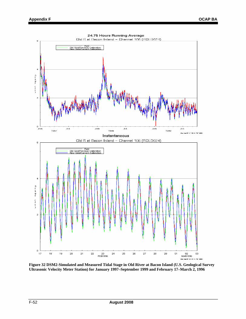
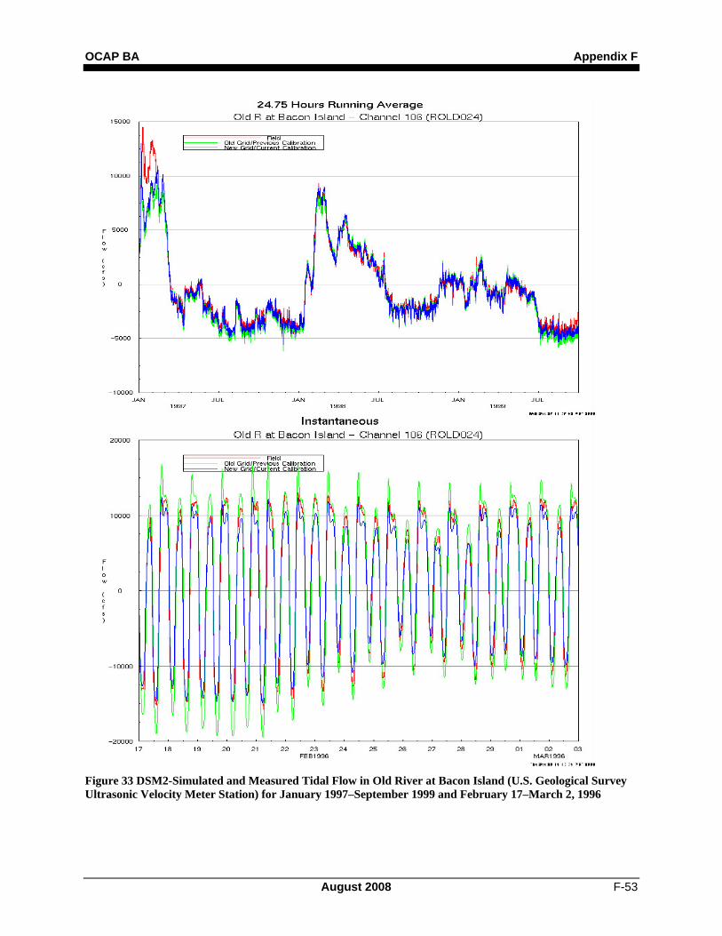
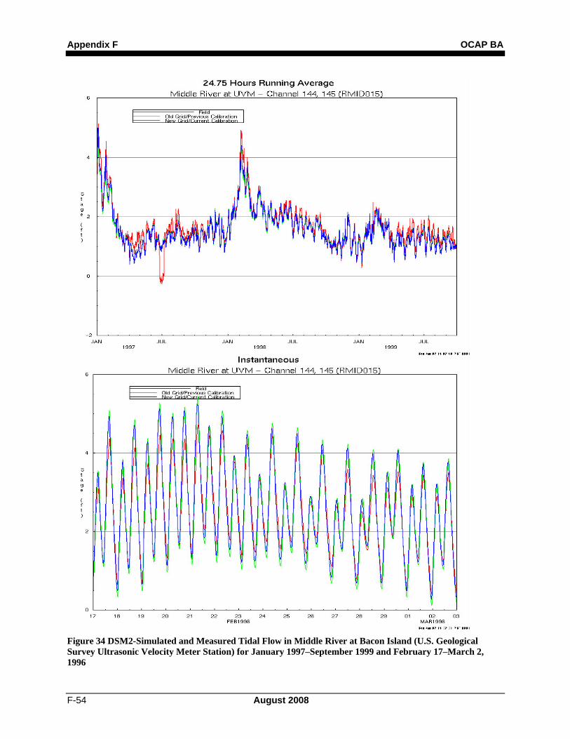
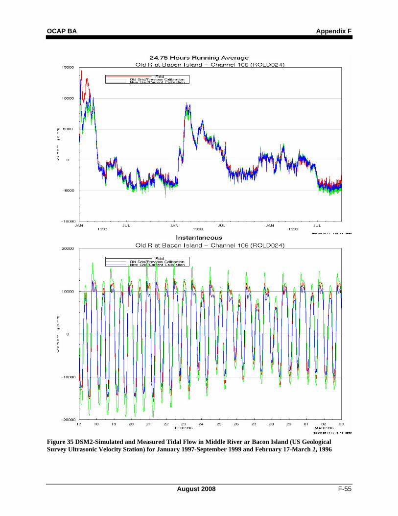
For Old River at Bacon Island, at the USGS UVM tidal flow station, Figure 32 shows the simulated and measured tidal stage and Figure 33 shows the simulated and measured tidal flows. The simulated daily average tidal stage matches the measured tidal stage of between 1 and 4 feet NGVD. The simulated tidal stage variations during the February 1996 high-flow event match the measured tidal stage data very well, although the simulated high tides are about 0.5 foot higher than measured. The range of simulated net flows in Old River at Bacon Island is about –5,000 cfs (net upstream flow) to about 10,000 cfs. The simulated tidal flow variations during the February 1996 high-flow event match the measured tidal flows well, with a range of –15,000 to 10,000 cfs before the high flow and –10,000 to 10,000 cfs during the peak flow. For Middle River at Bacon Island, at the USGS UVM tidal flow station, Figure 34 shows the simulated and measured tidal stage and Figure 35 shows the simulated and measured tidal flows. The simulated daily average tidal stage matches the measured tidal stage of between 1 and 4 feet NGVD. The simulated tidal stage variations during the February 1996 high-flow event match the measured stage data very well, although the simulated high tides are about 0.5 foot higher than measured. The range of simulated net flows in Middle River at Bacon Island is about –5,000 cfs (net upstream flow) to about 10,000 cfs. The simulated tidal flow variations during the February 1996 high-flow event match the measured tidal flows well, with a range of –15,000 to 10,000 cfs before the high flow and –10,000 to 10,000 cfs during the peak flow. The similarity of the tidal flows in Old and Middle River is remarkable. The calibrated DSM2 is properly simulating this nearly equal division of net and tidal flows between Old River and Middle River channels.

Appendix F OCAP BA

F-52 August 2008

Figure 32 DSM2-Simulated and Measured Tidal Stage in Old River at Bacon Island (U.S. Geological Survey Ultrasonic Velocity Meter Station) for January 1997–September 1999 and February 17–March 2, 1996

OCAP BA Appendix F

August 2008 F-53

Figure 33 DSM2-Simulated and Measured Tidal Flow in Old River at Bacon Island (U.S. Geological Survey Ultrasonic Velocity Meter Station) for January 1997–September 1999 and February 17–March 2, 1996

Appendix F OCAP BA

F-54 August 2008

Figure 34 DSM2-Simulated and Measured Tidal Flow in Middle River at Bacon Island (U.S. Geological Survey Ultrasonic Velocity Meter Station) for January 1997–September 1999 and February 17–March 2, 1996

OCAP BA Appendix F

August 2008 F-55

Figure 35 DSM2-Simulated and Measured Tidal Flow in Middle River ar Bacon Island (US Geological Survey Ultrasonic Velocity Station) for January 1997-September 1999 and February 17-March 2, 1996

Appendix F OCAP BA

F-56 August 2008

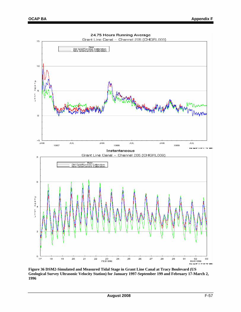
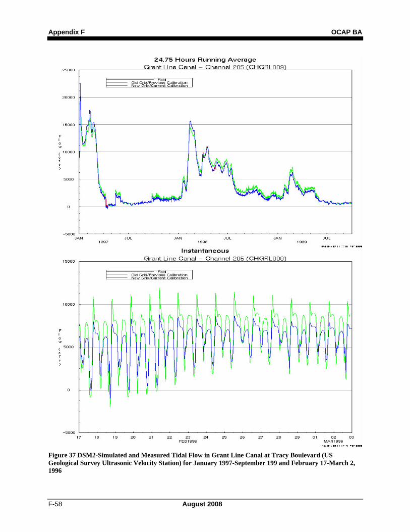
For Grant Line Canal at Tracy Boulevard Bridge, Figure 36 shows the simulated and measured tidal stage and Figure 37 shows the simulated and measured tidal flows. The simulated daily average tidal stage with the new calibration now matches the measured tidal stage of 6 feet at a flow of 15,000 cfs. The tidal stage variations during the February 1996 high-flow event match the measured tidal stage data reasonably well. The range of simulated net flows in Old River at the Tracy Boulevard Bridge is about 0–20,000 cfs. Most of the flow entering the south Delta from the head of Old River diversion from the San Joaquin River flows down the Grant Line Canal. The simulated tidal flows are somewhat irregular, with a pulse flood tide flow and a more steady ebb tide flow. During the February 1996 high-flow event, the tidal flows varied from 2,500 to 7,500 cfs.

OCAP BA Appendix F

August 2008 F-57

Figure 36 DSM2-Simulated and Measured Tidal Stage in Grant Line Canal at Tracy Boulevard (US Geological Survey Ultrasonic Velocity Station) for January 1997-September 199 and February 17-March 2, 1996

Appendix F OCAP BA

F-58 August 2008

Figure 37 DSM2-Simulated and Measured Tidal Flow in Grant Line Canal at Tracy Boulevard (US Geological Survey Ultrasonic Velocity Station) for January 1997-September 199 and February 17-March 2, 1996

OCAP BA Appendix F

August 2008 F-59

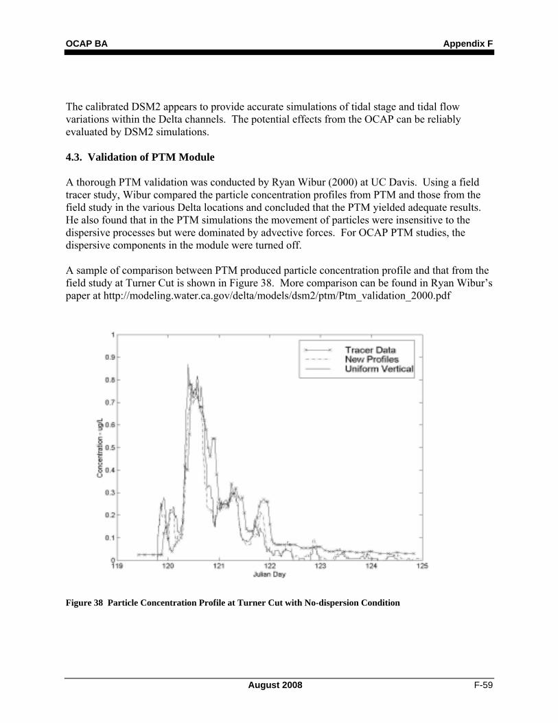
The calibrated DSM2 appears to provide accurate simulations of tidal stage and tidal flow variations within the Delta channels. The potential effects from the OCAP can be reliably evaluated by DSM2 simulations. 4.3. Validation of PTM Module A thorough PTM validation was conducted by Ryan Wibur (2000) at UC Davis. Using a field tracer study, Wibur compared the particle concentration profiles from PTM and those from the field study in the various Delta locations and concluded that the PTM yielded adequate results. He also found that in the PTM simulations the movement of particles were insensitive to the dispersive processes but were dominated by advective forces. For OCAP PTM studies, the dispersive components in the module were turned off. A sample of comparison between PTM produced particle concentration profile and that from the field study at Turner Cut is shown in Figure 38. More comparison can be found in Ryan Wibur’s paper at http://modeling.water.ca.gov/delta/models/dsm2/ptm/Ptm_validation_2000.pdf

Figure 38 Particle Concentration Profile at Turner Cut with No-dispersion Condition

Appendix F OCAP BA

F-60 August 2008

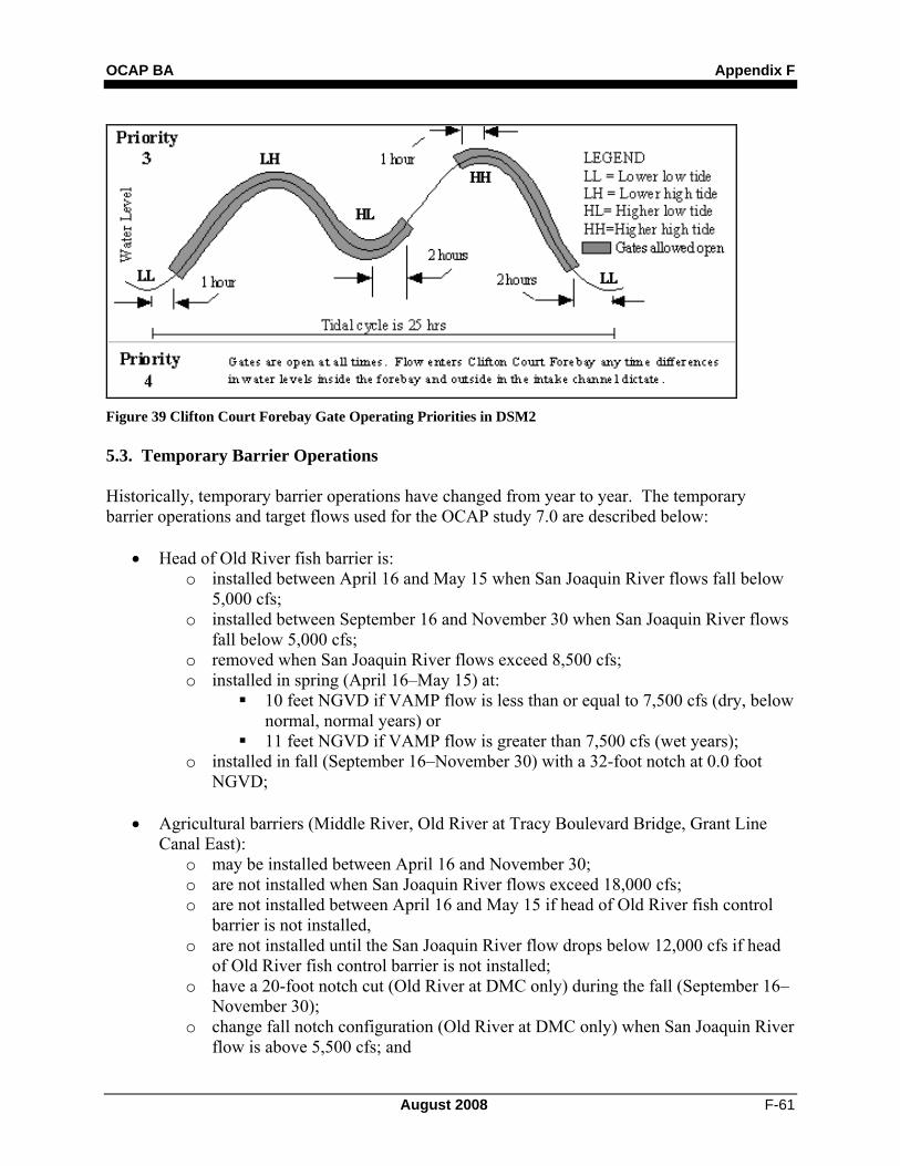
5. Input Assumptions for OCAP Studies Input assumptions and characteristics for the DSM2 16-year planning studies for OCAP are described below 5.1. Input data The modeling for OCAP-BA used a simulation time period of 1976 to 1991. There has been work to expand this time period to span an 82 year period (1922 to 2003). However, version 7, the newest incarnation of the DSM2 model suite incorporates some additional capabilities and was used for the OCAP-BA studies. The main benefit to using the latest version was the dynamic gate operations that are imbedded in the model. The new gate logic allows the operation of gates based on various hydraulic triggers rather than having to run the model iteratively. Unfortunately this new version has not been thoroughly tested with the 82 year time period. Since this analysis is only looking at hydrodynamics and particle movement, the variety of inflows and exports should be adequately captured by the 16 years (1976 to 1991) of simulation. Additional years of simulation may be important for salinity where antecedent conditions have a longer lasting affect. However for hydrodynamics little can be gained from a larger time period. 5.1. Vernalis Adaptive Management Plan Flows for San Joaquin River and SWP Banks and CVP Tracy Exports (VAMP) VAMP modifies San Joaquin River flows and SWP Banks and CVP Tracy export rates to enhance anadromous fish migration. Components of VAMP include a 31-day flow pulse in the San Joaquin River from April 15 to May 15 and corresponding reductions in exports at the SWP Banks and CVP Tracy during this time period. CALSIM II accounts for VAMP in its computations; however, the final (cycle 5 results) monthly outputs for the San Joaquin River at Vernalis, SWP Banks, and CVP Tracy do not reflect the VAMP flows and exports. Thus, for all OCAP studies, the CALSIM II results were post-processed to produce input data for DSM2 that include the VAMP pulse flow and reduced CVP Tracy and SWP Banks exports (from cycle 2 results). 5.2. Clifton Court Forebay Operations (CCF OP) DSM2 can simulate the operation of the CCF intake gates in a variety of ways known as priorities (Figure 39). For the OCAP studies, the CCF was operated tidally using Priority 3.

OCAP BA Appendix F

August 2008 F-61

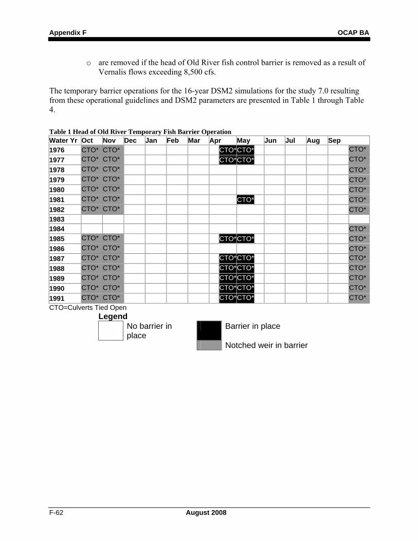
Figure 39 Clifton Court Forebay Gate Operating Priorities in DSM2 5.3. Temporary Barrier Operations Historically, temporary barrier operations have changed from year to year. The temporary barrier operations and target flows used for the OCAP study 7.0 are described below:

• Head of Old River fish barrier is: o installed between April 16 and May 15 when San Joaquin River flows fall below

5,000 cfs; o installed between September 16 and November 30 when San Joaquin River flows

fall below 5,000 cfs; o removed when San Joaquin River flows exceed 8,500 cfs; o installed in spring (April 16–May 15) at:

10 feet NGVD if VAMP flow is less than or equal to 7,500 cfs (dry, below normal, normal years) or

11 feet NGVD if VAMP flow is greater than 7,500 cfs (wet years); o installed in fall (September 16–November 30) with a 32-foot notch at 0.0 foot

NGVD;

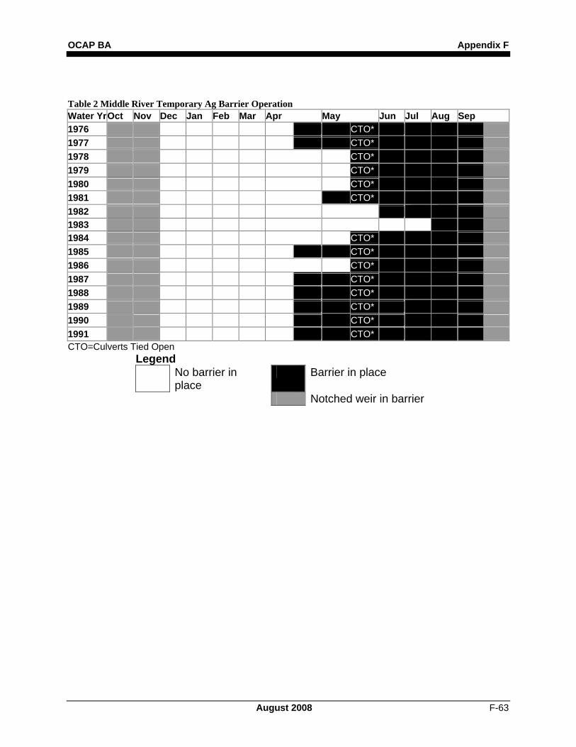
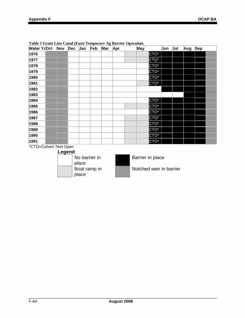
• Agricultural barriers (Middle River, Old River at Tracy Boulevard Bridge, Grant Line Canal East):

o may be installed between April 16 and November 30; o are not installed when San Joaquin River flows exceed 18,000 cfs; o are not installed between April 16 and May 15 if head of Old River fish control

barrier is not installed, o are not installed until the San Joaquin River flow drops below 12,000 cfs if head

of Old River fish control barrier is not installed; o have a 20-foot notch cut (Old River at DMC only) during the fall (September 16–

November 30); o change fall notch configuration (Old River at DMC only) when San Joaquin River

flow is above 5,500 cfs; and

Appendix F OCAP BA

F-62 August 2008

o are removed if the head of Old River fish control barrier is removed as a result of Vernalis flows exceeding 8,500 cfs.

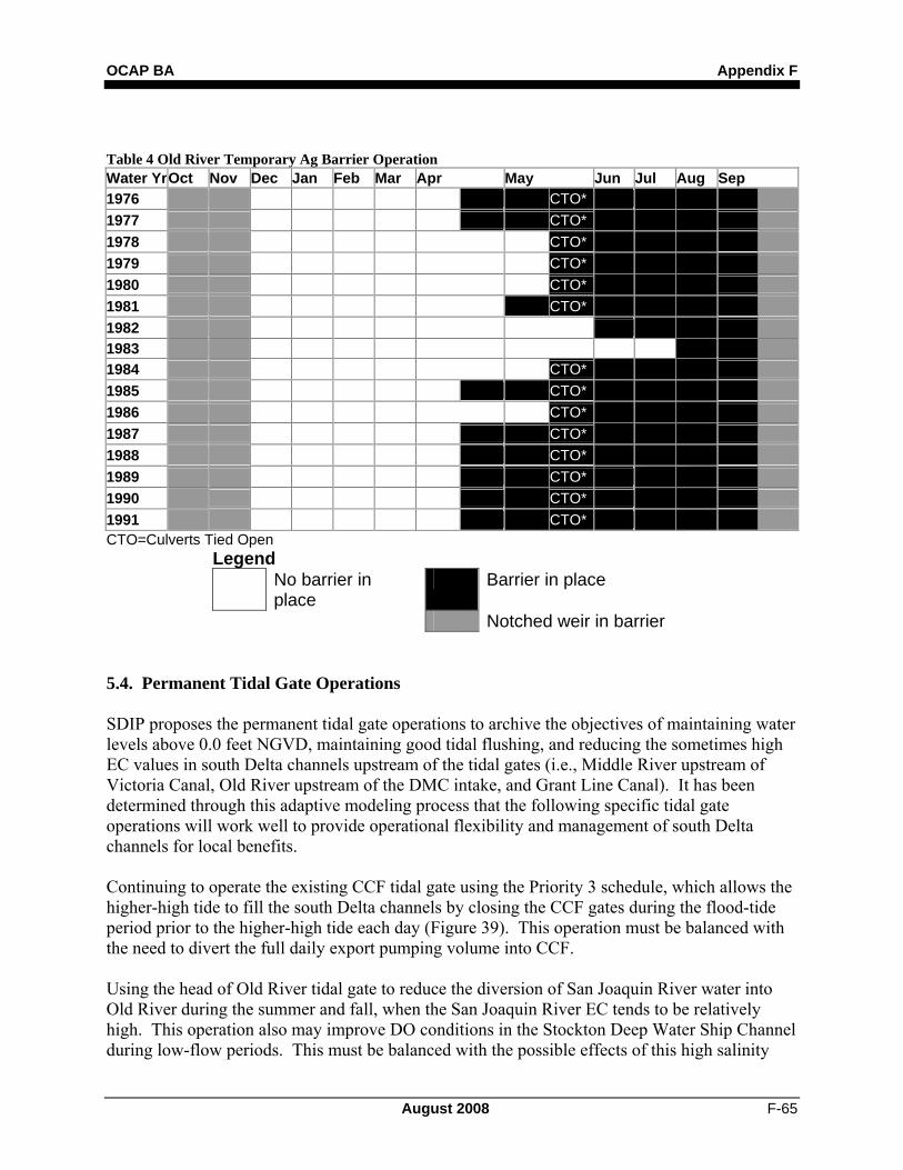
The temporary barrier operations for the 16-year DSM2 simulations for the study 7.0 resulting from these operational guidelines and DSM2 parameters are presented in Table 1 through Table 4. Table 1 Head of Old River Temporary Fish Barrier Operation Water Yr Oct Nov Dec Jan Feb Mar Apr May Jun Jul Aug Sep 1976 CTO* CTO* CTO*CTO* CTO*1977 CTO* CTO* CTO*CTO* CTO*1978 CTO* CTO* CTO*1979 CTO* CTO* CTO*1980 CTO* CTO* CTO*1981 CTO* CTO* CTO* CTO*1982 CTO* CTO* CTO*1983 1984 CTO*1985 CTO* CTO* CTO*CTO* CTO*1986 CTO* CTO* CTO*1987 CTO* CTO* CTO*CTO* CTO*1988 CTO* CTO* CTO*CTO* CTO*1989 CTO* CTO* CTO*CTO* CTO*1990 CTO* CTO* CTO*CTO* CTO*1991 CTO* CTO* CTO*CTO* CTO*CTO=Culverts Tied Open

Legend No barrier in

place Barrier in place

Notched weir in barrier

OCAP BA Appendix F

August 2008 F-63

Table 2 Middle River Temporary Ag Barrier Operation Water Yr Oct Nov Dec Jan Feb Mar Apr May Jun Jul Aug Sep 1976 CTO* 1977 CTO* 1978 CTO* 1979 CTO* 1980 CTO* 1981 CTO* 1982 1983 1984 CTO* 1985 CTO* 1986 CTO* 1987 CTO* 1988 CTO* 1989 CTO* 1990 CTO* 1991 CTO* CTO=Culverts Tied Open

Legend No barrier in

place Barrier in place

Notched weir in barrier

Appendix F OCAP BA

F-64 August 2008

Table 3 Grant Line Canal (East) Temporary Ag Barrier Operation Water Yr Oct Nov Dec Jan Feb Mar Apr May Jun Jul Aug Sep 1976 CTO* 1977 CTO* 1978 CTO* 1979 CTO* 1980 CTO* 1981 CTO* 1982 1983 1984 CTO* 1985 CTO* 1986 CTO* 1987 CTO* 1988 CTO* 1989 CTO* 1990 CTO* 1991 CTO* *CTO=Culvert Tied Open

Legend No barrier in

place Barrier in place

Boat ramp in place

Notched weir in barrier

OCAP BA Appendix F

August 2008 F-65

Table 4 Old River Temporary Ag Barrier Operation Water Yr Oct Nov Dec Jan Feb Mar Apr May Jun Jul Aug Sep 1976 CTO* 1977 CTO* 1978 CTO* 1979 CTO* 1980 CTO* 1981 CTO* 1982 1983 1984 CTO* 1985 CTO* 1986 CTO* 1987 CTO* 1988 CTO* 1989 CTO* 1990 CTO* 1991 CTO* CTO=Culverts Tied Open

Legend No barrier in

place Barrier in place

Notched weir in barrier 5.4. Permanent Tidal Gate Operations SDIP proposes the permanent tidal gate operations to archive the objectives of maintaining water levels above 0.0 feet NGVD, maintaining good tidal flushing, and reducing the sometimes high EC values in south Delta channels upstream of the tidal gates (i.e., Middle River upstream of Victoria Canal, Old River upstream of the DMC intake, and Grant Line Canal). It has been determined through this adaptive modeling process that the following specific tidal gate operations will work well to provide operational flexibility and management of south Delta channels for local benefits. Continuing to operate the existing CCF tidal gate using the Priority 3 schedule, which allows the higher-high tide to fill the south Delta channels by closing the CCF gates during the flood-tide period prior to the higher-high tide each day (Figure 39). This operation must be balanced with the need to divert the full daily export pumping volume into CCF. Using the head of Old River tidal gate to reduce the diversion of San Joaquin River water into Old River during the summer and fall, when the San Joaquin River EC tends to be relatively high. This operation also may improve DO conditions in the Stockton Deep Water Ship Channel during low-flow periods. This must be balanced with the possible effects of this high salinity

Appendix F OCAP BA

F-66 August 2008

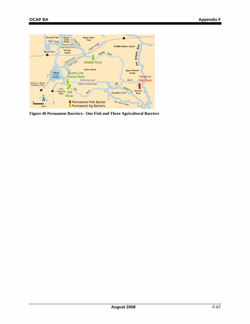
water shifting from the CVP exports to the SWP exports and CCWD diversions, as well as the planned Stockton diversion. Opening (lowering) the three agricultural gates during all periods of flood tide to provide the maximum possible flushing of the south Delta channels upstream of these gates. During the ebb tide, the gates are either partly or complete closed to protect water levels and to promote circulations in South Delta. Refer to Table 7 for more details of how individual gates are operated depending on San Joaquin flows and the time year. More details about the DSM2 modeling assumptions used in OCAP studies 7.0 and 8.0 are described below. Head of Old River Permanent Fish Tidal Gate The permanent fish control gate at the head of Old River was closed from April 15 to May 15 and almost completely closed from October 1 to November 30 of every year unless monthly average San Joaquin River flows at Vernalis exceed 10,000 cfs. The closure was assumed to be complete in April and May, although the actual fish control gate may have some flow through the fish ladder or passage feature (i.e., submerged opening) that is designed for adult fish migration passage. The head of Old River gate operation during the summer period of June–September was simulated by assuming that a diversion of 500 cfs would be regulated by partial gate closure, whenever the San Joaquin River flow was between 800 cfs and 2,500 cfs. Permanent Agricultural Tidal Gates Three permanent agricultural tidal gates are proposed:

• a Middle River gate near the confluence of Middle River and Victoria Canal, • a Grant Line Canal gate at the west end of the canal (the temporary Grant Line Canal

barrier is at the east end of the canal), and • an Old River gate near the DMC (Figure 40).

These tidal gates will be able to be opened or closed to allow water to pass upstream of the gates during rising tides and to prevent water levels upstream of the gates from dropping below a target water level during receding tides.

OCAP BA Appendix F

August 2008 F-67

Figure 40 Permanent Barriers: One Fish and Three Agricultural Barriers

Permanent Fish Barrier Permanent Ag Barriers

Head of Old River

Middle River

Old River

Grant Line Canal West

Appendix F OCAP BA

F-68 August 2008

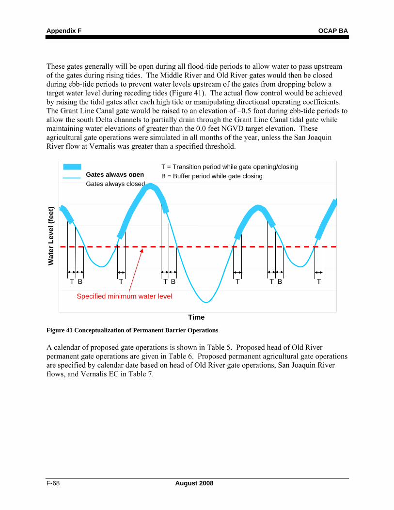
These gates generally will be open during all flood-tide periods to allow water to pass upstream of the gates during rising tides. The Middle River and Old River gates would then be closed during ebb-tide periods to prevent water levels upstream of the gates from dropping below a target water level during receding tides (Figure 41). The actual flow control would be achieved by raising the tidal gates after each high tide or manipulating directional operating coefficients. The Grant Line Canal gate would be raised to an elevation of –0.5 foot during ebb-tide periods to allow the south Delta channels to partially drain through the Grant Line Canal tidal gate while maintaining water elevations of greater than the 0.0 feet NGVD target elevation. These agricultural gate operations were simulated in all months of the year, unless the San Joaquin River flow at Vernalis was greater than a specified threshold.

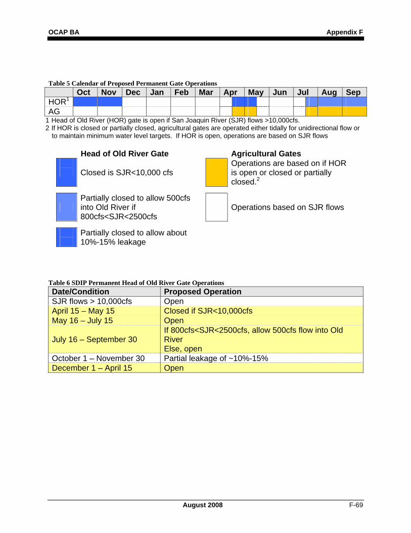
Figure 41 Conceptualization of Permanent Barrier Operations A calendar of proposed gate operations is shown in Table 5. Proposed head of Old River permanent gate operations are given in Table 6. Proposed permanent agricultural gate operations are specified by calendar date based on head of Old River gate operations, San Joaquin River flows, and Vernalis EC in Table 7.

Time

Wat

er L

evel

(fee

t)

Gates always open Gates always closed

T = Transition period while gate opening/closing B = Buffer period while gate closing

T B T T B T T B T

Specified minimum water level

OCAP BA Appendix F

August 2008 F-69

Table 5 Calendar of Proposed Permanent Gate Operations Oct Nov Dec Jan Feb Mar Apr May Jun Jul Aug Sep HOR1 AG

1 Head of Old River (HOR) gate is open if San Joaquin River (SJR) flows >10,000cfs. 2 If HOR is closed or partially closed, agricultural gates are operated either tidally for unidirectional flow or

to maintain minimum water level targets. If HOR is open, operations are based on SJR flows

Head of Old River Gate Agricultural Gates Closed is SJR<10,000 cfs

Operations are based on if HOR is open or closed or partially closed.2

Partially closed to allow 500cfs into Old River if 800cfs<SJR<2500cfs

Operations based on SJR flows

Partially closed to allow about 10%-15% leakage

Table 6 SDIP Permanent Head of Old River Gate Operations Date/Condition Proposed Operation SJR flows > 10,000cfs Open April 15 – May 15 Closed if SJR<10,000cfs May 16 – July 15 Open

July 16 – September 30 If 800cfs<SJR<2500cfs, allow 500cfs flow into Old River Else, open

October 1 – November 30 Partial leakage of ~10%-15% December 1 – April 15 Open

Appendix F OCAP BA

F-70 August 2008

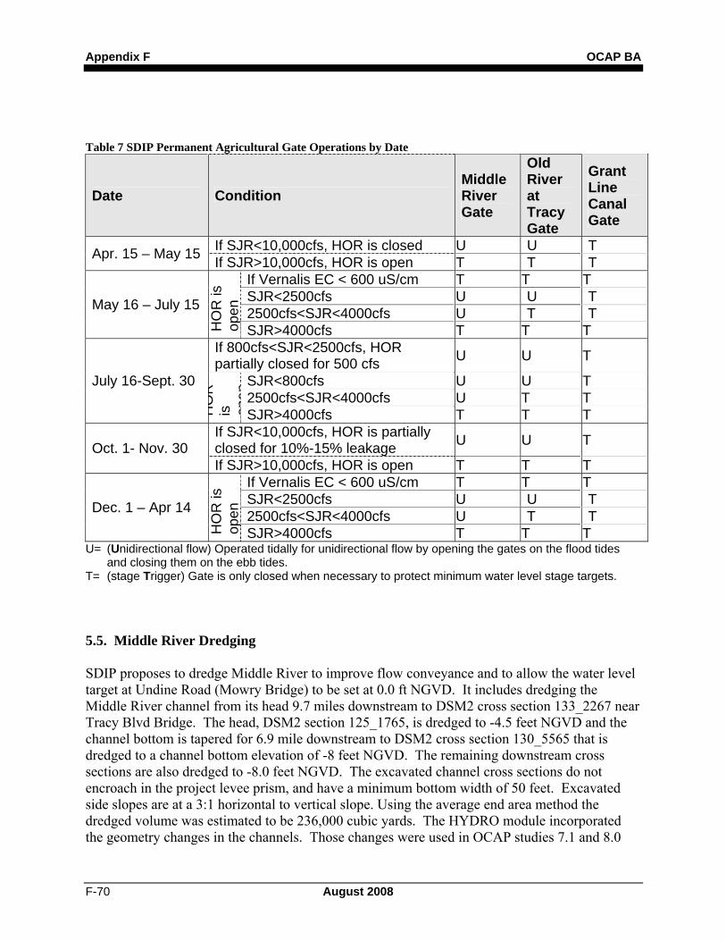
Table 7 SDIP Permanent Agricultural Gate Operations by Date

Date Condition Middle River Gate

Old River at Tracy Gate

Grant Line Canal Gate

If SJR<10,000cfs, HOR is closed U U T Apr. 15 – May 15 If SJR>10,000cfs, HOR is open T T T If Vernalis EC < 600 uS/cm T T T SJR<2500cfs U U T 2500cfs<SJR<4000cfs U T T May 16 – July 15

HO

R is

op

en

SJR>4000cfs T T T If 800cfs<SJR<2500cfs, HOR partially closed for 500 cfs U U T

SJR<800cfs U U T 2500cfs<SJR<4000cfs U T T

July 16-Sept. 30

HO

R

is

open

SJR>4000cfs T T T If SJR<10,000cfs, HOR is partially closed for 10%-15% leakage U U T Oct. 1- Nov. 30 If SJR>10,000cfs, HOR is open T T T

If Vernalis EC < 600 uS/cm T T T SJR<2500cfs U U T 2500cfs<SJR<4000cfs U T T Dec. 1 – Apr 14

HO

R is

op

en

SJR>4000cfs T T T U= (Unidirectional flow) Operated tidally for unidirectional flow by opening the gates on the flood tides

and closing them on the ebb tides. T= (stage Trigger) Gate is only closed when necessary to protect minimum water level stage targets. 5.5. Middle River Dredging SDIP proposes to dredge Middle River to improve flow conveyance and to allow the water level target at Undine Road (Mowry Bridge) to be set at 0.0 ft NGVD. It includes dredging the Middle River channel from its head 9.7 miles downstream to DSM2 cross section 133_2267 near Tracy Blvd Bridge. The head, DSM2 section 125_1765, is dredged to -4.5 feet NGVD and the channel bottom is tapered for 6.9 mile downstream to DSM2 cross section 130_5565 that is dredged to a channel bottom elevation of -8 feet NGVD. The remaining downstream cross sections are also dredged to -8.0 feet NGVD. The excavated channel cross sections do not encroach in the project levee prism, and have a minimum bottom width of 50 feet. Excavated side slopes are at a 3:1 horizontal to vertical slope. Using the average end area method the dredged volume was estimated to be 236,000 cubic yards. The HYDRO module incorporated the geometry changes in the channels. Those changes were used in OCAP studies 7.1 and 8.0

OCAP BA Appendix F

August 2008 F-71

5.6. Delta Cross Channel Gate Operations (DCC) The same operations were used for the Delta Cross Channel gates for all DSM2 simulations (studies 7.0, 7.1, 8.0). For months in which the gates were open for part of the month, DSM2 simulated that gate as open starting on the first day of the month and closed after the designated number of days. For example, in December 1975, the gates were open for the first 16 days of the month (December 1–16) and closed for the remainder of the month, starting on December 17. 5.7. DICU In DSM2, DICU is represented by three components:

• irrigation diversions from channels onto Delta islands, • drainage and return flows from Delta islands into the surrounding channels, and • seepage.

Thus, the net DICU is computed by the following relationship:

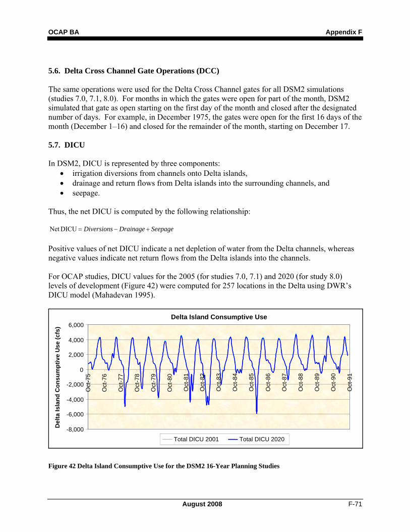
SeepageDrainageDiversions +−=DICUNet Positive values of net DICU indicate a net depletion of water from the Delta channels, whereas negative values indicate net return flows from the Delta islands into the channels. For OCAP studies, DICU values for the 2005 (for studies 7.0, 7.1) and 2020 (for study 8.0) levels of development (Figure 42) were computed for 257 locations in the Delta using DWR’s DICU model (Mahadevan 1995). Delta Island Consumptive Use

-8,000

-6,000

-4,000

-2,000

0

2,000

4,000

6,000

Oct

-75

Oct

-76

Oct

-77

Oct

-78

Oct

-79

Oct

-80

Oct

-81

Oct

-82

Oct

-83

Oct

-84

Oct

-85

Oct

-86

Oct

-87

Oct

-88

Oct

-89

Oct

-90

Oct

-91

Del

ta Is

land

Con

sum

ptiv

e U

se (c

fs)

Total DICU 2001 Total DICU 2020

Figure 42 Delta Island Consumptive Use for the DSM2 16-Year Planning Studies

Appendix F OCAP BA

F-72 August 2008

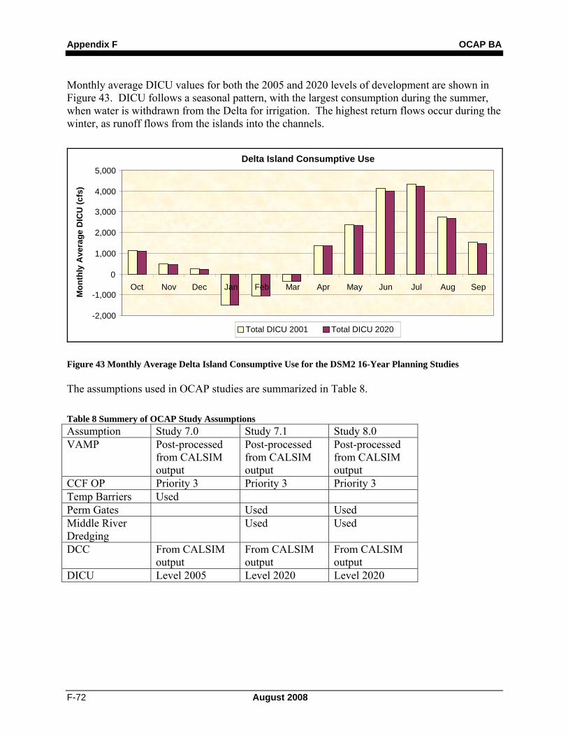
Monthly average DICU values for both the 2005 and 2020 levels of development are shown in Figure 43. DICU follows a seasonal pattern, with the largest consumption during the summer, when water is withdrawn from the Delta for irrigation. The highest return flows occur during the winter, as runoff flows from the islands into the channels.

Delta Island Consumptive Use

-2,000

-1,000

0

1,000

2,000

3,000

4,000

5,000

Oct Nov Dec Jan Feb Mar Apr May Jun Jul Aug Sep

Mon

thly

Ave

rage

DIC

U (c

fs)

Total DICU 2001 Total DICU 2020

Figure 43 Monthly Average Delta Island Consumptive Use for the DSM2 16-Year Planning Studies The assumptions used in OCAP studies are summarized in Table 8. Table 8 Summery of OCAP Study Assumptions Assumption Study 7.0 Study 7.1 Study 8.0 VAMP Post-processed

from CALSIM output

Post-processed from CALSIM output

Post-processed from CALSIM output

CCF OP Priority 3 Priority 3 Priority 3 Temp Barriers Used Perm Gates Used Used Middle River Dredging

Used Used

DCC From CALSIM output

From CALSIM output

From CALSIM output

DICU Level 2005 Level 2020 Level 2020

OCAP BA Appendix F

August 2008 F-73

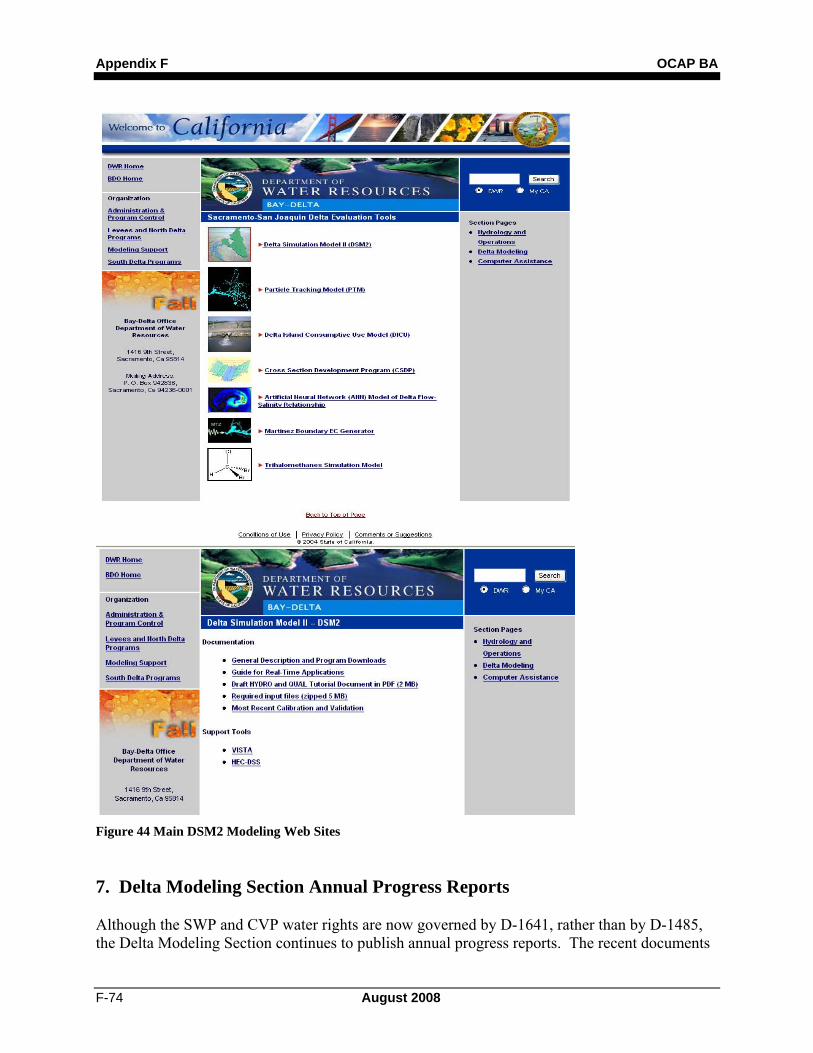
6. DSM2 Documentation There is not a printed users manual or model documentation report. There is, however, considerable information about DSM2 available on the DWR Delta Modeling website at: http://baydeltaoffice.water.ca.gov/modeling/deltamodeling/deltaevaluation.cfm. This website (shown in Figure 44) has links to information about:

• the main modules of DSM2, hydrology (HYDRO), and water quality (QUAL); • the PTM, which uses output from the hydrology module of DSM2; • the DICU model, which can be used to develop inputs to DSM2; • the Cross Section Development Program, which can be used to develop channel

geometry inputs to DSM2; • the ANN model of Delta flow-salinity relationships, an alternative to using DSM2 for

estimating Delta salinity; • Martinez boundary EC generator, which can be used to estimate inputs to DSM2; • a trihalomethanes simulation model; and • the DSM2 Users Group.

The link to DSM2 takes the viewer to the DSM2 web page. The DSM2 web page (also shown in Figure 44) has links to information on model use, including a DSM2 tutorial. Other links lead to model code, executable files, and model inputs. This web page also has a link to information about Vista, a program developed by DWR to view data that are stored in the HEC-DSS format. Many of the model inputs are in this format. Data in the HEC-DSS format can also be imported and viewed in Excel using a DSS add-in for Excel that is available from the HEC website at: http://www.hec.usace.army.mil/software/hec-dss/hecdss_msexcel_addin.htm. This add-in also allows for the creation of DSS files from Excel tables. This add-in greatly facilitates the editing and creation of input data files and the viewing of model results.

Appendix F OCAP BA

F-74 August 2008

Figure 44 Main DSM2 Modeling Web Sites 7. Delta Modeling Section Annual Progress Reports Although the SWP and CVP water rights are now governed by D-1641, rather than by D-1485, the Delta Modeling Section continues to publish annual progress reports. The recent documents

OCAP BA Appendix F

August 2008 F-75

are available from the DWR Delta Modeling website. The chapters that directly describe the DSM2 modeling system are listed below to facilitate further study:

• 1994 (15th) Annual Report—Chapter 2, “New Model Development (DSM2-HYDRO and DSM2-QUAL);”

• 1995 (16th) Annual Report—Chapter 3, “Water Quality (DSM2-QUAL),” and Chapter 4, “Particle Tracking (DSM2-PTM);”

• 1997 (18th) Annual Report—Chapter 2, “DSM2 Model Development” (html format for website);

• 1998 (19th) Annual Report—Chapter 5, “DSM2 Input and Output,” and Chapter 6, “Cross-Section Development Program (CSDP);”

• 1999 (20th) Annual Report—Chapter 4, “Modeling of 1998 Hydrodynamics in the Delta (comparison to UVM stations);”

• 2000 (21st) Annual Report—Chapter 8, “Filling In and forecasting DSM2 Tidal Boundary Level;”

• 2001 (22nd) Annual Report—Chapter 2, “DSM2 Calibration and Validation” (also see www.iep.water.ca.gov/dsm2pwt/dsm2pwt.html), Chapter 7, “Integration of CALSIM and ANN models for Delta Flow-Salinity Relationships,” Chapter 10, “Planning Tide at the Martinez Boundary,” Chapter 11, “Improving Salinity Estimates at the Martinez Boundary,” and Chapter 12, “DSM2 Real-Time Forecasting System;”

• 2002 (23rd) Annual Report—Chapter 12, “DSM2 Documentation,” Chapter 13, “DSM2 Input Database and Data Management System,” and Chapter 14, “DSM2 Fingerprinting Methodology;”

• 2003 (24th) Annual Report—Chapter 6, “New Behaviors and Control switches in DSM2-PTM,” and Chapter 7, “Implementation of a new DOC growth (source) algorithm in DSM2-QUAL;” and

• 2004 (25th) Annual Report—Chapter 3, “DSM2 Geometry Investigations,” Chapter 6, “Net Delta Outflow Computations for DSM2 Steady State Simulations,” Chapter 7, “Extensions and Improvements to DSM2,” and Chapter 12, “Calculating Clifton Court Forebay Inflow.”

References Anderson, J., and M. Mierzwa. 2002. Section 6.5 Gates: An introduction to modeling flow

barriers in DSM2. Pages 164–168 in DSM2 tutorial—an introduction to the Delta Simulation Model II (DSM2) for simulation of hydrodynamics and water quality of the Sacramento–San Joaquin Delta. Draft. February. Delta Modeling Section, Office of State Water Project Planning, California Department of Water Resources. Sacramento, CA.

Ateljevich, E. 2001a. Chapter 10: Planning tide at the Martinez boundary. In Methodology for flow and salinity estimates in the Sacramento-San Joaquin Delta and Suisun Marsh. August. 22nd Annual Progress Report to the State Water Resources Control Board. California Department of Water Resources. Sacramento, CA.

Ateljevich, E. 2001b. Chapter 11: Improving salinity estimates at the Martinez boundary. In Methodology for flow and salinity estimates in the Sacramento-San Joaquin Delta and

Appendix F OCAP BA

F-76 August 2008

Suisun Marsh. August. 22nd Annual Progress Report to the State Water Resources Control Board. California Department of Water Resources. Sacramento, CA

California Department of Water Resources. 2002. Appendix D: CALSIM ANN Implementation. Pages 120–129 in Benchmark studies assumptions. September 30. Bay-Delta Office, Modeling Support Branch.

California Department of Water Resources. 1985a. The Department of Water Resources planning simulation model for California. Division of Planning. Sacramento, CA.

California Department of Water Resources. 1985b. Map: Flood Channel Design Flows. May. California Department of Water Resources.

Delong, L.L., D.B. Thompson, and J.K. Lee. 1993. Computer program FourPt, a model for simulating one-dimensional, unsteady, open channel flow. Unpublished manual. Stennis Space Center, MS: U.S. Geological Survey, Water Resources Division.

Denton, R.A. 1993. Accounting for antecedent conditions in seawater intrusion modeling—applications to the San Francisco Bay-Delta. ASCE Hydraulic Engineering Conference 1993.

Delta Simulation Model Version 2 Project Work Team. 2001. Chapter 7: DSM2 Geometry Development. In Enhanced calibration of DSM2 HYDRO and QUAL. Draft. November. Prepared for the Interagency Ecological Program for the Sacramento–San Joaquin Estuary. Sacramento, CA.

Fischer, H.B. 1982. DELFLO and DELSAL, flow and transport models for the Sacramento–San Joaquin Delta, description and steady-state verification. Report HBF 82/01. Berkeley, CA.

Mahadevan, N. 1995. Estimation of Delta island diversions and return flows. California Department of Water Resources, Division of Planning. February. Sacramento, CA.

Nader-Tehrani, P. 2001. Chapter 9: Use of repeating tides in planning runs. In Methodology for flow and salinity estimates in the Sacramento-San Joaquin Delta and Suisun Marsh. 22nd Annual Progress Report to the State Water Resources Control Board. California Department of Water Resources. Sacramento, CA. August 2001. Available: < http://modeling.water.ca.gov/ delta/reports/annrpt/2001/2001Ch9.html>. Last revised: October 1, 2001.

Oltmann, R.N. 1998. Measurement of Delta outflow using ultrasonic velocity meters and comparison with mass-balance calculated outflow. Interagency Ecological Program for the Sacramento–San Joaquin Estuary Newsletter 11 (1). Winter.

Oltmann, R.N., M.R. Simpson. 1997. Measurement of tidal flows in the Sacramento–San Joaquin Delta, California. U.S. Geological Survey poster presentation. Available: <http://sfbay.wr.usgs.gov/access/delta/tidalflow/ uvmstations2.html>. Last revised: January 12, 1999.

Simpson, M.R., and R.N. Oltmann. 1993. Discharge measurement using an acoustic Doppler current profiler. U.S. Geological Survey Water-Supply Paper 2395, 34 p

Ryan Wilbur 2000, Validation of dispersion using the particle tracking model in the Sacramento-San Joaquin Delta, Davis California. Master’s thesis. Available: http://modeling.water.ca.gov/delta/models/dsm2/ptm/Ptm_validation_2000.pdf