appendix d - variance components + random effects in … components and random effects ... consider...
TRANSCRIPT

APPENDIX D
Variance components and random effects
models in MARK . . .
Kenneth P. Burnham, USGS Colorado Cooperative Fish & Wildlife Research Unit
The objectives of this appendix are
• to introduce to biologists the concept and nature of what are called (alternative names
for the same essential idea) ‘variance components’, ‘random effects’, ‘random coefficient
models’, or ‘empirical Bayes estimates’
• present the basic theory and methodology for fitting simple random effects models,
including shrinkage estimators, to capture-recapture data (i.e.,Cormack-Jolly-Seberand
band or tag recovery models)
• extend AIC to simple random effects models embedded into the otherwise fixed-effects
capture-recapture likelihood.
• develop some proficiency in executing a variance components analysis and fitting
random effects model in program MARK
Much of the conceptual material presented in this appendix is derived from a paper authored by
Kenneth Burnham and Gary White (2002) – hereafter, we will refer to this paper as ‘B&W’. It is assumed
that the reader already has a basic knowledge of some standard encounter-mark-reencounter models
as described in detail in this book (e.g., dead recovery and live recapture models – referred to here
generically as ‘capture-recapture’).
We introduce the subject of – and some of the motivation for – this appendix by example. In the
following we consider two relatively common scenarios (out of a much larger set of possibilities) where
a ‘different analytical approach’ might be helpful.
Scenario 1 – parameters as random samples
Consider a Cormack-Jolly-Seber (CJS) time-specific model {St pt} wherein survival (S) and capture
probabilities (p) are allowed to be time varying for (k + 2) capture occasions, equally spaced in time.
If k ≥ 20 we are adding many survival parameters into our model as if they were unrelated; however,
more parsimonious models are often needed. Consider a reduced parameter model – at the extreme,
we have the model {S· pt } wherein S1 � S2 � · · · � Sk � S·. However, this model may not fit well
even if the general (time-dependent) CJS model fits well and there is no evidence of any explainable
© Cooch & White (2018) 04.17.2018

D - 2
structural time variation, such as a linear time trend, in this set of survival rates, or variation as a function
of an environmental covariate. Instead, there may be unstructured time variation in the Si that is not
easily modeled by any simple smooth parametric form, yet which cannot be wisely ignored. In this case
it is both realistic and desirable to conceptualize the actual unknown Si as varying, over these equal-
length time intervals, about a conceptual population mean E(S) � µ, with some population variation,
σ2 (Fig. D.1).
Figure D.1: Schematic representation of variation in occasion-specific parameters θi , as if the parameters were
drawn randomly from some underlying distribution with mean µ and variance σ2.
Here, by population, we will mean a conceptual statistical distribution of survival probabilities, such
that the Si may be considered as a sample from this distribution. Hence, we proceed as if Si are a random
sample from a distribution with mean µ and variance σ2. Doing so can lead to improved inferences
on the Si regardless of the truth of this conceptualization if the Si do in fact vary in what seems
like a random, or exchangeable, manner. The parameter σ2 is now the conventional measure of the
unstructured variation in the Si, and we can usefully summarize S1 . . . Sk by two parameters: µ and σ2.
The complication is that we do not know the Si; we have only estimates Si , subject to non-ignorable
sampling variances and covariances, from a capture-recapture model wherein we traditionally consider
the Si as fixed, unrelated parameters. We would like to estimate µ and σ2, and adjust our estimates to
account for the different contributions to the overall variation in our estimates due to sampling, and the
environment. For this, we consider a random effects model.
Scenario 2 – separating sampling + environmental (process) variation
Precise and unbiased estimation of parameter uncertainly (say, the SE of the parameter estimate) is
critical to analysis of stochastic demographic models. Consider for example, the estimation of the risk
of extinction. It is well known (and entirely intuitive) that any simply stochastic process (say, growth
of an age- or size-structured population through time) is more likely to go extinct the more variable a
particular ‘vital rate’ is (say, survival or fertility). Thus, if an estimate of the variance of a parameter is
Appendix D. Variance components and random effects models in MARK . . .

D.1. Variance components – some basic background theory D - 3
biased high, then this tends to bias high the probability of extinction. We wish to use only estimates of
environmental (or process) variation alone, excluding sampling variation, since it is only the magnitude
of the former that we want to include in our viability models (White 2000).
Precise estimation of process variation is also critical for analysis of the relationship of the variation
of a particular demographic parameter to the projected growth of a population. The process variation
in projected growth, λ, is a function of the process variance of a particular demographic parameter. To
first order, and assuming no covariances between the ai j elements, this can be expressed as
var(λ) ≈∑
i j
(∂λ
∂ai j
)var(ai j).
From this expression, we anticipate that natural selection will select against high process variation in
a parameter that λ is most ‘sensitive’ to (i.e., for which ∂λ/∂ai j is greatest) (Pfister 1998; Schmutz 2009).
Thus, robust estimation of the process variance of fitness components is critical for life history analysis.
In this appendix, we will consider estimation of variance components, and fitting of random effects
models, using program MARK. We begin with the development of some of the underlying theory,
followed by illustration of the ‘mechanics’ of using program MARK, by means of a series of ‘worked
examples’.
D.1. Variance components – some basic background theory
The basic idea is relatively simple. We imagine that the Si are distributed randomly about E(S) � µ
(Fig. D.1). The variation in Si is σ2, as if S1, . . . Sk are a sample from a population. It is not required
that the sampling be random – merely that the S1, . . . , Sk are exchangeable (or, more formally, that the
conceptual residuals (µ−Si) should appear like an iid sample,with no remaining structural information).
There are no required distributional assumptions, such as normality.
If we knew the Si then it follows that
E(S) � S σ2�
∑k(Si − S)2
k − 1.
Of course, except in a computer simulation, we rarely if ever know the Si. What we might have are ML
estimates Si, and estimates of conditional variation var(Si
�� Si
).
We can express our estimate of Si in standard linear form as the sum of the mean µ, the deviation of
the Si from the mean, δi , and the error term ǫi
Si � µ + δi + ǫi ,
where δi � (Si − µ) and ǫi � (Si − Si). Substituting into our expression for Si,
Si � µ + δi + ǫi
� µ + (Si − µ)︸ ︷︷ ︸↑ σ2
(processvariance)
+ (Si − Si).︸ ︷︷ ︸↑ var(Si |Si )(samplingvariance)
Here (and hereafter) we distinguish between ‘process’ (or, environmental) variation, σ2, and ‘sampling’
Appendix D. Variance components and random effects models in MARK . . .

D.1. Variance components – some basic background theory D - 4
variation, var(Si
�� Si
). We refer to the sum of process and sampling variation as total variation, σ2
total .
total variation � σ2total � process variation + sampling variation
� σ2+ var
(Si
�� Si
).
It is important to note that sampling variation, var(Si
�� Si
), depends on the sample size of animals
captured, whereas process variance σ2 does not. It is also important to note that if there is sampling
covariation, then this should be included in our expression for total variance, σ2total :
σ2total � σ
2+
[E(var
(Si
�� Si
) )+ E
(cov
(Si , S j
�� Si , S j
)) ].
For fully time-dependent models, the sampling covariances of Si and S j are often very small for many
of the data types we work with in MARK, especially relative to process and sampling variance, and the
covariance term can often be ignored. We will do so now, for purposes of simplifying the presentation
somewhat, but will return to the issue of sampling covariances later on.
If we assume for the moment that all the sampling variances are equal, then the estimate of the overall
mean survival is just the mean of the k estimates:
¯S �
∑k Si
k,
with the theoretical variance being the sum of process and sampling variance divided by k:
var( ¯S
)�
σ2+ E
[var
(Si
�� Si
) ]k
.
Our interest generally lies in estimation of the process variation. By algebra, we see that process
variance can be estimated by, in effect, subtracting the sampling variation from the total variation.
σ2total � process variation + sampling variation
� σ2+ var
(Si
�� Si
)∴ σ2
� σ2total − var
(Si
�� Si
).
Hence, we need an estimate for σ2total and var
(Si
�� Si
).
If we assume that S1, . . . , Sk are a random sample, with S � E(S), and population variance σ2, then
from general least-squares theory
¯S �
∑k wi Si∑k wi
,
where
wi �1
σ2+ var
(Si
�� Si
) .
Appendix D. Variance components and random effects models in MARK . . .

D.1. Variance components – some basic background theory D - 5
Given wi , the theoretical variance of ˆS is
var( ¯S
)�
1∑k wi
.
However, although var(Si
�� Si
)is estimable, we would still need to know σ2.
An alternative approach which leads to an empirical (data-based) estimator is
var( ¯S
)�
∑k wi
(Si − ¯S
)2
(∑k wi
) (k − 1
) .
We note that if there is no process variation (σ2� 0), then the above reduces to the familiar case of k
replicates.
More generally, if we assume that the weights, wi are equal (or nearly so), then we can re-write the
empirical estimator as
var( ¯S
)�
∑k (Si − ¯S)2
(k − 1), if wi � w, ∀i
where
¯S �
∑k Si
k.
The assumption that the weights, wi are equal is generally reasonable if (i) the var(Si
�� Si
)are all
nearly equal, or if (ii) they are all small, relative to σ2. In theory, when the Si vary, then the var(Si
�� Si
)will also vary. In contrast, with low sampling effort, such that var
(Si
�� Si
)is much larger than process
variance σ2, it might be sufficient to use the approximation
wi �1
var(Si
�� Si
) .
In this case, only relative weights wi would be needed (since an estimate of σ2 is not needed).
Now, assume for the moment we are interested in estimating the process variation around the mean
S. If we also assume that there is no sampling covariance, and that wi � w, and∑k wi � 1, then we
estimate the total variance as
σ2total � var
( ¯S)�
∑k (Si − ¯Si
)2
(k − 1),
and the sampling variance as the mean of the estimated sample variances
E[var
(Si
�� Si
) ]�
∑k var(Si
�� Si
)k
.
Hence, our estimate of process variance would be
σ2�
∑k−1 (Si − ¯Si
)2
k − 1−
∑k var(Si
�� Si
)k
.
Appendix D. Variance components and random effects models in MARK . . .

D.1. Variance components – some basic background theory D - 6
However, this estimator (which is essentially the estimator described by Gould & Nichols 1998) is not
entirely correct (or efficient). It was derived under the strong assumption that the sampling variances
are all equal (i.e., that SE(Si) are all identical). In practice, this is usually not the case, and thus we refer
to the preceding as a ‘naïve’ estimator of process variance.
Instead, we need to weight them to obtain an unbiased estimate of σ2. As noted earlier, general least-
squares theory suggests using a weight wi
wi �1
σ2+ var
(Si
�� Si
) .Hence, the estimator of the weighted mean survival is
¯S �
∑k wi Si∑k wi
,
with theoretical variance
var( ¯S
)�
1∑k wi
,
and empirical variance estimator
var( ¯S
)�
∑k wi
(Si − ¯S
)2[∑k wi
] (k − 1
) .
When the wi are the true (but unknown) weights, we have
1∑k wi
�
∑k wi
(Si − ¯S
)2[∑k wi
](k − 1)
,
which if we normalize the weights (such that they sum to 1), gives
1 �
∑k wi
(Si − ¯S
)2
(k − 1).
Since
wi �1
σ2+ var
(Si
�� Si
) and ¯S �
∑k wi Si∑k wi
,
then
1 �
∑k wi
(Si − ¯S
)2
(k − 1) �
k∑ 1
σ2+ var
(Si
�� Si
)(Si −
k∑.
1
σ2+ var
(Si
�� Si
) Si
)2(k − 1)
Appendix D. Variance components and random effects models in MARK . . .

D.2. Variance components estimation – worked examples D - 7
We then solve (numerically) for σ2 (which is the only unknown in the expression) – it is convenient
to use the naïve estimate for σ2 calculated earlier as a starting point in the numerical optimization.
A confidence interval can be constructed for σ2 by solving two modified versions of this equation.
We assume we want a (1 − α)% CI, where α � αU + αL (where U and L stand for upper and lower,
respectively). For the upper limit, we solve for σ2 in the following
k∑ 1
σ2+ var
(Si
�� Si
)(Si −
k∑ 1
σ2+ var
(Si
�� Si
) Si
)2(k − 1) �
χ2k−1,αL
k − 1,
where χ2n−1,αL
is the critical value for the central χ2 distribution corresponding to (k − 1) df and αL
percentile.
To find the lower limit, we substitute χ2k−1,1−αU
in the RHS of the preceding, and solve for σ2. If the
lower limit does not have a positive solution for σ2 (since σ ≥ 0), then we set the lower CI to 0 and adjust
to a one-sided CI by redefining αU � α.
Burnham et al. (1987) describe simplified versions of these estimators for the CI if all the var(Si
�� Si
)are the same, or nearly so.
D.2. Variance components estimation – worked examples
Here, we introduce the ‘mechanics’ of the variance decomposition, using a series of progressively more
complex examples. We begin with a simple example loosely based on a ‘known fate’ analysis, where
survival is estimated as a simple binomial probability, and where there is no covariance among samples.
D.2.1. Binomial survival – simple mean (no sampling covariance)
Imagine a simulated scenario where we are conducting a simple ‘known fate’ analysis (Chapter 16). In
each of 10 years (k � 10), we mark and release n � 25 individuals, and determine the number alive, y,
after 1 year (since this is a known-fate analysis, we assume there is no error in determining whether
an animal is ‘alive’ or ‘not alive’ on the second sampling occasion). Here, though, we’ll assume that
the survival probability in each year, Si , is drawn from N(0.5, 0.05) (i.e., distributed as an independent
normal random variable with mean µ � 0.5 and process variance σ2� 0.052).
Conditional on each Si , we generated yi (number alive after one year in year i) as an independent
binomial random variable B(n, Si). Thus, our ML estimate of survival for each year is Si � yi/n, with
a conditional sampling variance of var(Si
�� Si
)� [Si(1 − Si)]/n, which given µ � 0.5, and σ2
� (0.05)2is approximately 0.01.
Table D.1 (top of the next page) gives the values of Si , yi and Si for our ‘example data’. Clearly, for a
‘real analysis’, we would not know the true values for Si – we would have only Si, and generally only
have ES
(var
(Si
�� Si
) )as var
(Si
�� Si
).
In Table D.1 we see that the empirical standard deviation of the 10 estimated survival rates (i.e., the Si)
is 0.106. However, we should not take (0.106)2 as an estimate of σ2 because such an estimate includes
both process and sampling variation. Clearly, we want to subtract the estimated sampling variance from
the total variation to get an estimate of the overall process variation.
Appendix D. Variance components and random effects models in MARK . . .

D.2.1. Binomial survival – simple mean (no sampling covariance) D - 8
Table D.1: Single realization from simple binomial survival example, k � 10, E(S) � 0.5, σ � 0.05, whereSi � yi/n are B(25, Si), hence expected SE(Si |S) ≈ 0.1
year (i) Si Si SE(Si
�� Si
)1 0.603 0.640 0.096
2 0.467 0.360 0.096
3 0.553 0.480 0.100
4 0.458 0.440 0.100
5 0.506 0.480 0.100
6 0.498 0.320 0.093
7 0.545 0.600 0.098
8 0.439 0.400 0.098
9 0.488 0.560 0.099
10 0.480 0.560 0.099
mean 0.504 0.484 0.100
SD 0.050 0.106
Using the manual approach...
From section D.1, if we make the strong assumption that all the sampling variances are equal, then the
estimate of the overall mean is the mean of the k estimates:
¯S �
∑k Si
k,
with the theoretical variance being
var( ¯S
)�
σ2+ E
[var
(Si
�� Si
) ]k
.
In other words the total variance is the sum of the process (environmental) variance, σ2, plus the
expected sampling variance, E[var
(Si
�� Si
) ].
From section D.1, and assuming equal weights wi , where∑k
� 1, we estimate the total variance as
var( ¯S
)�
∑k (Si − ¯Si
)2
(k − 1),
and the expected sampling variance as the mean of the sampling variances
E[var
(Si
�� Si
) ]�
∑k var(Si
�� Si
)k
.
Appendix D. Variance components and random effects models in MARK . . .

D.2.1. Binomial survival – simple mean (no sampling covariance) D - 9
Thus, we can derive an estimate of the process (environmental) variance σ2 by algebra
σ2�
10∑(Si − ¯Si
)2
(10 − 1)−
10∑var
(Si
��� Si
)10
.
Thus, from Table (D.1), the process variance for our k � 10 samples is estimated as
σ2�
10∑(Si − ¯Si
)2
(10 − 1)−
10∑var
(Si
��� Si
)10
�
(0.10064
9
)− 0.00959
� 0.0016
∴ σ �√
0.0016 � 0.040.
While our estimate of process variance is not much different from the true underlying value (for this
example, true σ2� 0.0025), we noted that this naïve estimator is not entirely correct, since it assumes
equal sampling variances. To obtain an unbiased estimate of σ2, we weight the sampling variance by
wi �1
σ2+ var
(Si
�� Si
) .From section D.1, we derive an estimate of process variance over the k � 10 samples by solving
(numerically) the following for σ2
1 �
10∑wi
(Si − ¯S
)2
(10 − 1)
�
10∑ 1
σ2+ var
(Si
�� Si
) ©«Si −
10∑wi Si
10∑wi
ª®®®¬
2
(10 − 1)
�
10∑ 1
σ2+ var
(Si
�� Si
)(Si −
10∑ 1
σ2+ var(Si |Si)
Si
)2(10 − 1)
.
For the present example, our estimated process variance is σ2� 0.00195.
Now, using MARK...
While estimating process variance ‘by hand’ is relatively straightforward for this example, we are clearly
interested in using the capabilities of program MARK to handle the ‘heavy lifting’ – especially for more
Appendix D. Variance components and random effects models in MARK . . .
D.2.1. Binomial survival – simple mean (no sampling covariance) D - 10
complex problems. Here we will introduce some of the ‘mechanics’ in using program MARK to estimate
process variance for our simulated ‘known fate’ data. The data (number of marked and released animals
that survive the one-year interval; see Table D.1) are formatted for the ‘known fate’ data type, and are
contained in binomial-example.inp.
Since our purpose here is to demonstrate the mechanics of ‘variance components analysis’, and not
‘known fate analysis’, we’ve gone ahead and built the basic general model {St} for you. Start MARK, and
open up binomial-example.dbf (note: you’ll need to have binomial-example.fpt installed in the same
directory where you have binomial-example.dbf). There is only one model in the browser (for now) –
model ‘S(t) -- general model’. [At some point, you should look at the underlying PIM structure, to
see how we are using the known fate data type to model survival using a simple binomial estimator.]
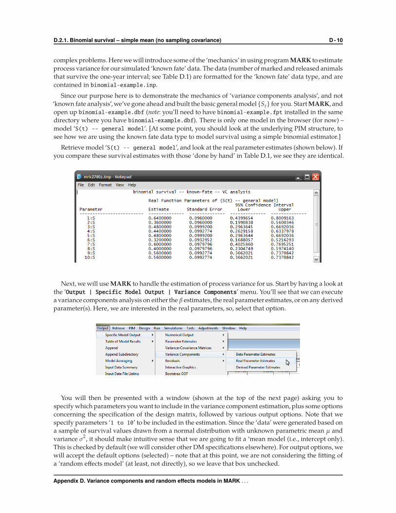
Retrieve model ‘S(t) -- general model’, and look at the real parameter estimates (shown below). If
you compare these survival estimates with those ‘done by hand’ in Table D.1, we see they are identical.
Next, we will use MARK to handle the estimation of process variance for us. Start by having a look at
the ’Output | Specific Model Output | Variance Components’ menu. You’ll see that we can execute
a variance components analysis on either the β estimates, the real parameter estimates, or on any derived
parameter(s). Here, we are interested in the real parameters, so, select that option.
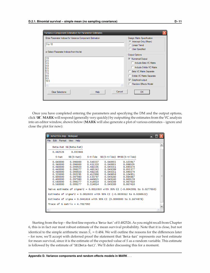
You will then be presented with a window (shown at the top of the next page) asking you to
specify which parameters you want to include in the variance component estimation, plus some options
concerning the specification of the design matrix, followed by various output options. Note that we
specify parameters ‘1 to 10’ to be included in the estimation. Since the ‘data’ were generated based on
a sample of survival values drawn from a normal distribution with unknown parametric mean µ and
variance σ2, it should make intuitive sense that we are going to fit a ‘mean model (i.e., intercept only).
This is checked by default (we will consider other DM specifications elsewhere). For output options, we
will accept the default options (selected) – note that at this point, we are not considering the fitting of
a ‘random effects model’ (at least, not directly), so we leave that box unchecked.
Appendix D. Variance components and random effects models in MARK . . .
D.2.1. Binomial survival – simple mean (no sampling covariance) D - 11
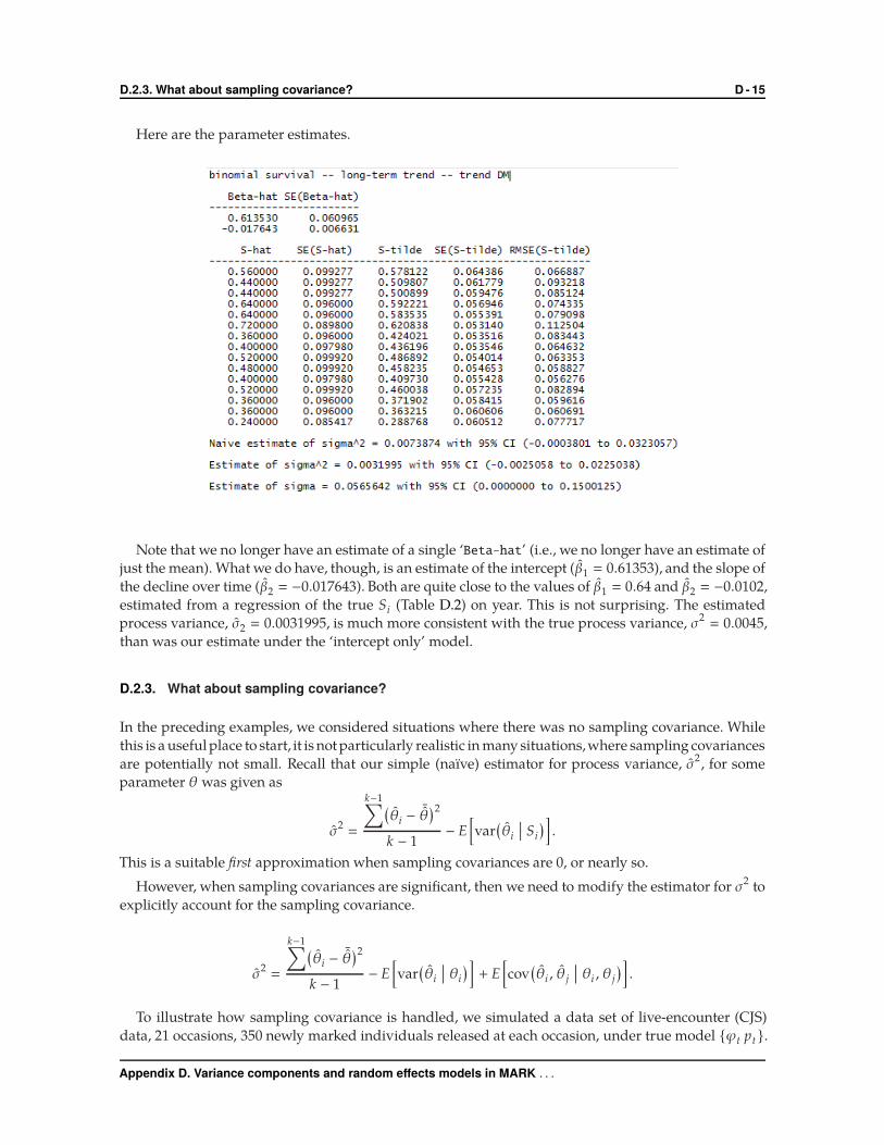
Once you have completed entering the parameters and specifying the DM and the output options,
click ‘OK’. MARK will respond (generally very quickly) by outputting the estimates from the VC analysis
into an editor window, shown below (MARK will also generate a plot of various estimates – ignore and
close the plot for now):
Starting from the top – the first line reports a ‘Beta-hat’ of 0.482526. As you might recall from Chapter
6, this is in fact our most robust estimate of the mean survival probability. Note that it is close, but not
identical to the simple arithmetic mean ¯Si � 0.484. We will outline the reasons for the differences later
– for now, we’ll accept with deferred proof the statement that ‘Beta-hat’ represents our best estimate
for mean survival, since it is the estimate of the expected value of S as a random variable. This estimate
is followed by the estimate of ‘SE(Beta-hat)’. We’ll defer discussing this for a moment.
Appendix D. Variance components and random effects models in MARK . . .

D.2.2. Binomial example extended – simple trend D - 12
Next, a table of various parameter estimates. The first two columns should be self-explanatory –
the ML estimates of survival Si (‘S-hat’), followed by the binomial standard error for the estimate
(‘SE(S-hat)’. Next, the ‘shrinkage’ estimates Si (‘S-tilde’) and their corresponding SE and RMSE. The
derivation, use and interpretation of the shrinkage estimates is developed in section D.3.
Finally, the estimates for process variation (the G matrix we’ll get to later). First, MARK reports the
‘naive estimate of sigma^2’= 0.001595. This is exactly the same value as the ‘first approximation’ we
derived ‘by hand’ in the preceding section. This is followed by the ‘Estimate of sigma^2’ = 0.0019503
(and the ‘Estimate of sigma’ = 0.044162). Both estimates are identical to those we derived ‘by hand’
using the ‘weighted means’ approach in the preceding section.
Now, about the ‘SE(Beta-hat)’ noted above. For this example, in the absence of sampling covariance,
it is estimated as the square-root of the sum of estimated process variation, σ2, and sampling variation,
E[var
(Si
�� Si
) ], divided by k, where k is the number of parameter estimates. For our present example,
with k � 10,
‘SE(Beta-hat)’ �
√σ2
+ E[var
(Si
�� Si
) ]k
�
√(0.0019503+ 0.0095872)
10� 0.03396,
which is what is reported by MARK (to within rounding error). Thus, our estimate of total variance
(i.e., the value of the numerator inside the square-root) would be (SE2 × k) � (0.033962 × 10) � 0.01153.
The ‘SE(Beta-hat)’ is useful for calculating 95% CI for ‘Beta-hat’. For this example, we can construct
a reasonable CI for ‘Beta-hat’ as 0.482526± (1.96 × 0.033946) → [0.4160, 0.5491].
D.2.2. Binomial example extended – simple trend
Here we consider a similar scenario, again involving a simple ‘known fate’ analysis with no sampling
covariance among samples. In each of 15 years (k � 15), we mark and release n � 25 individuals,
and determine the number alive, y, after 1 year. Here, though, we assume that the true mean survival
probability in each year, Si , is declining over time (from 0.60 in the first year, to 0.46 in the final year).
We’ll assume that the survival probability in each year, Si, is drawn from N(Si , 0.05). Conditional on
each Si , we generated yi (number alive after one year in year i) as an independent binomial random
variable B(n, Si). Table D.2 (top of the next page) gives the values of Si , yi and Si for our ‘example data’.
Now, in the preceding example, the survival probability in each year, Si, was drawn from N(0.5, 0.05)(i.e., distributed as an independent normal random variable with mean µ � 0.5 and process variance
σ2� 0.052). Here, though, not only is there random variation around the mean, but the mean itself
declines over time. In this example there are 2 sources of process variation: the random variation around
the mean survival in any given year, and the decline over time in the value of the mean. As such, we
anticipate that the actual process variance will be > (0.05)2.∗ We also anticipate that if we estimate
process variance using a model based on a simple mean (i.e., where we assume that process variation
is due only to variation around a mean survival which is the same in all years) the estimate will be
biased high (since it will conflate within- and among-year sources of variation). What about sampling
variation? The imposition of a trend does not influence sampling variation – in each year, sampling is
based on a binomial with the same number of individuals ‘released’ each year.
∗ The actual value of the process variance, accounting for both within and among season variation, is σ2� 0.0045.
Appendix D. Variance components and random effects models in MARK . . .

D.2.2. Binomial example extended – simple trend D - 13
Table D.2: Single realization from simple binomial survival example, k � 15, S declining linearly from 0.6 → 0.46(S � 0.53), σ � 0.05, where Si � yi/n are B(25, Si) – hence expected SE
(Si
�� S)≈ 0.1.
year (i) Si Si SE(Si
�� Si
)1 0.647 0.560 0.00992 0.595 0.440 0.0099
3 0.667 0.440 0.0099
4 0.580 0.640 0.0092
5 0.532 0.640 0.0092
6 0.475 0.720 0.0081
7 0.624 0.360 0.0092
8 0.516 0.400 0.0096
9 0.640 0.520 0.0100
10 0.430 0.480 0.0100
11 0.503 0.400 0.0096
12 0.509 0.520 0.0100
13 0.533 0.360 0.0092
14 0.394 0.360 0.0092
15 0.490 0.240 0.0073
mean 0.542 0.472 0.0093SD 0.081 0.129
We’ll test both expectations, using data contained in binomial-example-trend.inp. Again, we’ve
provided you with some ‘pre-built’ models to start with (contained in binomial-example-trend.dbf
and binomial-example-trend.fpt). We’ll avoid doing the same ‘hand calculations’ we worked through
in the preceding example (same basic idea, but a fair bit messier because of having to account for both
within and among year variation), and simply use MARK.
Start MARK, and open up binomial-survival-trend.dbf. You’ll see that there are 2 ‘pre-built’
models in the browser: ‘S(t) - DM’ (simple time variation) and ‘S(T) - DM’ (a trend model, where
annual estimates are constrained to follow a linear trend). The ‘-DM’ simply indicates that both were
constructed using a design matrix. Based on AICc weights, there is clearly far more support for the
trend model (which is the true generating model) than the model with simple time variation.
Our purpose here is not to do ‘model selection’ (we’ll get there). Our present interest is on estimating
the variance components. So, first question. Which model do we want to estimate variance components
from? This is a more subtle question than it might seem. On the one hand, if we didn’t know there was
a trend, it might seem that we should select the time-dependent model since it is more general. On the
other hand, you might have prior information suggesting a trend, and might think that it is a better
model. Or, you might build both models, see that the trend model has the most support in the data, and
use that model as the basis for estimating variance components.
You need to think this through carefully. We are trying to estimate process variance – we want to
estimate the magnitude of the joint within- and among-year variation in our data. Thus, we want to use
the most general model possible. In this case, model ‘S(t) - DM’. We don’t use model ‘S(T) - DM’, since
the estimates from that model are constrained to fall on a straight line. Meaning, the only remaining
variation would be the annual variation in mean survival (as estimated by the regression equation).
Meaning, that any estimate of process variation from such a model would massively underestimate
true process variation in the data.
Appendix D. Variance components and random effects models in MARK . . .

D.2.2. Binomial example extended – simple trend D - 14
Start by retrieving model ‘S(t) - DM’. Then, select ‘Output | Specific model output | Variance
components | Real parameter estimates’. With 15 samples we specify ‘1 to 15’.
What about the ‘design matrix specification’? Recall from the preceding example that we used
the default ‘Intercept Only (mean)’ specification. However, there are 2 other options available to
you: ‘linear trend’, and ‘user specified’. In effect, the first 2 options (‘intercept only’ and ‘linear
trend’) are there simply for your convenience, since both models are very commonly used. You could,
however, build either model by selecting the ‘user specified’ option (which essentially is the option
you select if you want to build a specific model directly, using the design matrix). We’ll defer using
the ‘user specified’ option for now, and simply compare the ‘intercept only’ and ‘linear trend’
models. We’ll start with the default ‘intercept only’ option.
Once you click the ‘OK’ button, MARK will respond with the estimates of year-specific survival
probabilities, and the estimates of total and process variance (shown below). Again, the first line is
the estimate of the overall mean, ¯S � 0.4711, and SE � 0.0342 (representing total variance). Note that
the reported mean is very close to the mean of the true Si (Table D.2), Si � 0.472.
What about the estimated variance? The estimate of process variance σ2� 0.00825, which as we
anticipated is almost twice as large as the true process variance in the data (σ2� 0.0045). Thus, the
estimated SE for total variance will also be biased high.
Now, let’s do a variance components analysis on the time-dependent model, by checking the ‘linear
trend’ DM option, as shown below:
Appendix D. Variance components and random effects models in MARK . . .
D.2.3. What about sampling covariance? D - 15
Here are the parameter estimates.
Note that we no longer have an estimate of a single ‘Beta-hat’ (i.e., we no longer have an estimate of
just the mean). What we do have, though, is an estimate of the intercept (β1 � 0.61353), and the slope of
the decline over time (β2 � −0.017643). Both are quite close to the values of β1 � 0.64 and β2 � −0.0102,
estimated from a regression of the true Si (Table D.2) on year. This is not surprising. The estimated
process variance, σ2 � 0.0031995, is much more consistent with the true process variance, σ2� 0.0045,
than was our estimate under the ‘intercept only’ model.
D.2.3. What about sampling covariance?
In the preceding examples, we considered situations where there was no sampling covariance. While
this is a useful place to start, it is not particularly realistic in many situations,where sampling covariances
are potentially not small. Recall that our simple (naïve) estimator for process variance, σ2, for some
parameter θ was given as
σ2�
k−1∑(θi − ¯θ
)2
k − 1− E
[var
(θi
�� Si
) ].
This is a suitable first approximation when sampling covariances are 0, or nearly so.
However, when sampling covariances are significant, then we need to modify the estimator for σ2 to
explicitly account for the sampling covariance.
σ2�
k−1∑(θi − ¯θ
)2
k − 1− E
[var
(θi
�� θi
) ]+ E
[cov
(θi , θj
�� θi , θj
) ].
To illustrate how sampling covariance is handled, we simulated a data set of live-encounter (CJS)
data, 21 occasions, 350 newly marked individuals released at each occasion, under true model {ϕt pt }.
Appendix D. Variance components and random effects models in MARK . . .

D.2.3. What about sampling covariance? D - 16
Apparent survival, ϕi , over a given interval i was generated by selecting a random beta deviate drawn
from B(0.7, 0.005). The encounter probability pi at a sampling occasion i was generated by selecting
a random beta deviate drawn from B(0.35, 0.005). The simulated live-encounter data are contained in
normsim-VC.inp. The estimates ϕi from model {ϕt pt} are shown at the top of the next page. For a time-
dependent model, the terminal ϕ and p parameter estimates are confounded (reflected in the estimated
SE(ϕ20) � 0.000). This becomes important when we specify the parameters in the variance-components
analysis.
Estimation of σ2 under the naïve model is straightforward. The only additional complications are that
(i) the terms in the estimator are calculated over ϕ1 → ϕ19, and (ii) we have to calculate the mean of the
sample covariances to estimate E[cov
(ϕi , ϕ j
�� ϕi , ϕ j
) ]. In practice, this second step isn’t too difficult,
depending on your facility with computers. You simply need to find a way to calculate the mean of the
off-diagonal elements of the V-C matrix (keeping in mind you’re calculating the mean over ϕ1 → ϕ19).
For the present example, cov(ϕi , ϕ j
�� ϕi , ϕ j
)� −0.00008. Thus,
σ2�
k−1∑(ϕi − ¯ϕ
)2
k − 1− E
[var
(ϕi
�� ϕi
) ]+ E
[cov
(ϕi , ϕ j
�� ϕi , ϕ j
) ]
�
(0.11531
18
)−
(0.0338
19
)− 0.00008 � 0.004552.
Clearly, the proportional contribution of the covariance term is very small (2%). This will often be
the case, especially for time-dependent models.
If we analyze these live-encounter data using the variance components routines in MARK, using
the ‘intercept only’ mean model, the reported value for the ‘naïve’ estimate (shown at the top of the
next page) matches the value we derived by hand on the preceding page. The estimate based on the
‘weighted’ estimator is almost identical – and both are not too far off the true value of σ2� 0.005.
The near equivalence of the ‘naïve’ and ‘weighted’ estimates reflects the fact that sampling variation
is small, relative to process variance, in this example (small sampling variance is not surprising, given
that the data were generated under a model with p � 0.35 and 350 individuals marked and released on
Appendix D. Variance components and random effects models in MARK . . .

D.3. Random effects models and shrinkage estimates D - 17
each sampling occasion). Recall from section D.1 that from least-squares theory, we should weight our
estimates of total and sampling variance to obtain an unbiased estimate of process variance, σ2, using
a weight wi :
wi �1
σ2+ var
(ϕi
�� ϕi
) .For this example, var
(ϕi
�� ϕi
)≪ σ2 , ∀i, and so wi ≈ 1/σ2, which is a constant (since σ2 is a constant).
Thus, for this example, the weighting does not change the naïve estimate.
You may have noticed that the ML estimates (‘S-hat’) are very close to what we identified earlier as
‘shrinkage’ estimates (‘S-tilde’). Is the near-equivalence of the ‘naïve’ and ‘weighted’ estimates for σ2
related to the ‘closeness’ of the ML and ‘shrinkage’ estimates?
D.3. Random effects models and shrinkage estimates
In this section, we introduce what we will refer to as ‘random effects’ models. We’ll begin by having
another look at the results from the simple binomial example (section D.2.1):
From left to right are the ML estimates, Si (‘S-hat’), the estimated standard error for the ML estimate,
SE(Si
�� S)
(‘SE(S-hat)’), the corresponding ‘shrinkage’ estimate, Si (‘S-tilde’), the estimated standard
Appendix D. Variance components and random effects models in MARK . . .

D.3.1. The basic ideas... D - 18
error for the shrinkage estimate, SE(Si
�� Si
), and the estimated residual mean-squared error (RMSE) for
the shrinkage estimate, �RMSE(Si
�� Si
)(‘RMSE(S-tilde)’).
Here is a plot of the ML estimates, Si (green line), the ‘shrinkage’ estimates, Si (blue line), and the
model estimates (for the mean model, corresponding to the estimated mean β � 0.4825; red line).
We are familiar with the ‘ideas’ behind the ML estimates, Si, and the idea of an overall estimate of
the mean survival, E(S), hopefully makes some intuitive sense. But, what are ‘shrinkage’ estimates?
We’ll start with a short-form explanation, focussing on the basic ideas, then jump down into the weeds
a bit for a deeper (more technical) discussion. The concept of a ‘shrinkage’ estimate is perhaps not the
easiest thing to understand.∗ We will follow this by illustrating the mechanics of building and fitting
these models in MARK, through a series of ‘worked examples’.
D.3.1. The basic ideas...
Looking at the tabular output and the plot, there are notable differences in point estimates,and precision,
between the the ML estimates and the shrinkage estimates. If you look carefully, you’ll notice that
for most years, the shrinkage estimate falls somewhere between the ML estimate, and the mean. The
shrinkage method is so called because each residual arising from the fitted reduced-parameter model
(Si − E(S)) is ‘shrunken’, then added back to the estimated model structure for observation i under
that reduced model. In a heuristic sense, the Si are derived from the ML estimates by removal of the
sampling variation.
When sampling covariances are zero†, the shrinkage estimator used in MARK for the mean-only
model (although the structure applies generally) is
Si � E(S) +
√√√√ σ2
σ2+ ES
[var
(Si
�� Si
) ] ×[Si − E(S)
].
∗ In his definitive text on matrix population models, Hal Caswell comments that understanding eigenvalues and eigenvectors(which feature prominently in demographic analysis) requires ‘not only a mechanical understanding, but a real intuitive graspof the slippery little suckers...’ (p. 662, 2nd edition). We submit the same sentiment applies to ‘shrinkage’ estimates.
† The full shrinkage estimator, accounting for non-zero sampling covariances, is presented in section D.3.2.
Appendix D. Variance components and random effects models in MARK . . .

D.3.1. The basic ideas... D - 19
The first term on the right-hand side (RHS) of the expression is the estimate of the mean survival, E(S).The last term, [Si − E(S)], is simply the residual of the ML estimate from the model. But what about the
middle term on the RHS?
We will generally refer to √√√√ σ2
σ2+ ES
[var
(Si
�� Si
) ] ,as the ‘shrinkage coefficient’, and it clearly is a function of the proportion of total variance – i.e., the sum
σ2+ var
(Si
�� Si
)– due to process (environmental) variation, σ2. The square-root is used because then
σ2 .�
∑k (Si − ¯S)2
k − 1and E(S) .� ¯S.
If there is no process variation (i.e., σ2� 0), then the shrinkage coefficient is evaluated at 0, and thus
the shrinkage estimate would be the mean, E(S). In other words, if you have no environmental variation,
then the only variation in the system is sampling. If you remove the sampling variation (which we noted
earlier is what shrinkage is doing, at least heuristically), then this makes sense – without process or
sampling variation, every shrinkage estimate would simply be the mean, i.e., Si � E(S). In contrast, with
increasing process variance (i.e., increasing σ2), we see that as σ2 > var(Si
�� Si
)(i.e., as the proportion
of total variance due to process variance increases), then the shrinkage coefficient approaches 1.0, and
the shrinkage estimate would approach the ML estimate, Si .
This relationship is depicted in the following diagram where the arrows indicate the direction that
decreasing or increasing process variance σ2 has on the value of the shrinkage estimate, Si , relative to
the arithmetic average of the ML estimate Si and the mean E(S).
E(S) Si Si
↓ σ2
↑ σ2
Thus, another way of looking at it is to view the shrinkage estimate is analogous to an ‘average’
between the two estimates. This is important when we consider model averaging – we defer discussion
of that important topic until section D.5.
We should note that a shrinkage coefficient different than
√√√√ σ2
σ2+ ES
[var
(Si
�� Si
) ]
could be used. However, this particular shrinkage coefficient has a very desirable property: if we treat
the Si as if they were a random sample, then their sample variance almost exactly equals σ2. This also
means that a plot of the shrinkage residuals (as implicit in the plot at the top of the preceding page)
gives a correct visual image of the process variation in the Si .
This starts to point us in the direction of answering the basic question ‘why derive shrinkage
estimators for the Si?’. The answer in part comes from the observation we just made that the sample
variance of the shrinkage estimates is very close to the estimate of process variance, σ2. So, the shrinkage
estimates are ‘improved’, relative to the ML estimates, since they should have better precision. If we
look at the estimates for the binomial survival example, we see that the improvements gained by the
Appendix D. Variance components and random effects models in MARK . . .

D.3.1. The basic ideas... D - 20
shrinkage estimators, Si , appears substantial – they have about 50% better precision (simply compare
SE(Si
�� Si
)to SE
(Si
�� Si
)).
However, because the ML estimates are unbiased, and the shrinkage estimators are biased (as we will
explain), a necessary basis for a fair comparison is the sum of squared errors (SSE). The SSE is a natural
measure of the closeness of a set of estimates to the set of Si . For example, for the binomial survival
example, the SSE for the ML estimates is
SSEMLE �
10∑(Si − Si
)2� 0.067
while for the shrinkage estimates, the SSE is
SSEshr inka ge �
10∑(Si − Si
)2� 0.019
Clearly, in this sample the shrinkage estimates, as a set, are closer to truth. The expected SSE is the
mean square error, MSE (= E[SSE]), which is a measure of average estimator performance.
Those of you with some background in statistical theory might see the connections between the
preceding and James-Stein estimation, wherein (in highly simplified form) when 3 or more parameters
are estimated simultaneously, there exist combined estimators more accurate on average (that is, having
lower expected MSE) than any method that considers the parameters separately. For example, let θ is
a vector consisting of n ≥ 3 unknown parameters. To estimate these parameters, we take a single
measurement Xi for each parameter θi , resulting in a vector X of length n. Suppose the measurements
are independent, Gaussian random variables, such that X ∼ N(µ, 1). The most obvious approach to
parameter estimation would be to use each measurement as an estimate of its corresponding parameter:
θ � X. James-Stein demonstrated that this standard (LS) estimator is suboptimal in terms of mean
squared error, E(θ − θ). In other words, there exist alternative estimators which always achieve lower
mean squared error, no matter what the value of θ is. For example, it can be shown that a combined
estimator of the sample and global mean is a better predictor of the future than is the individual sample
mean, since the total MSE of the combined estimator is lower than if using the sample means themselves.
This clearly points to partof the theory underlying the use of shrinkage estimators – James-Stein says that
a combined estimator (say, of the ML estimate and the random mean, which is of course our shrinkage
estimate) will have a lower MSE than will the ML estimates themselves (with the degree of improvement
increasing with increasing number of sample means being combined).
It is important to note, however, that the combined estimator will be closer to optimal overall, since
it minimizes the MSE of the estimates overall. However, it is possible that any one individual estimate
could be ‘incorrectly shrunk’ (relative to the true value of the parameter), even in the wrong direction.
So, shrinkage is conceptually optimal for the set of parameters, but not necessarily for any individual
parameter).
If these ideas are new to you, papers by Efron & Morris (1975, 1977) are quite accessible, and provide
excellent introductions to the subject.
begin sidebar
Shrinkage estimators and 95% confidence limits
For the ML estimates, an approximate 95% confidence interval on Si is given by Si ±2 SE(Si
�� Si
). This
procedure will have good coverage in this example. However, for the shrinkage estimator if we use
Si ± 2 SE(Si
�� Si
), coverage will be negatively affected by the bias of S. Theory (discussed in B&W)
shows that the correct expected coverage occurs for the interval Si ± 2 �RSME(Si
�� Si
), where
Appendix D. Variance components and random effects models in MARK . . .

D.3.2. Some technical background... D - 21
�RSME(Si
�� Si
)�
√var
(Si
�� Si
)+
(Si − Si
)2.
The expectation over Si of �MSE(Si
�� Si
)�
[�RSME(Si
�� Si
) ]2is approximately the mean square
error for Si , MSEi . For the ML estimates,
�RSME(Si
�� Si
)� SE
(Si
�� Si
),
because Si is unbiased. The unbiasedness of the ML estimates in the general model, together with a
high correlation between Si and Si , and the assumption that Si are random, allows an argument that�RMSE(Si
�� Si
)is an estimator of the unconditional sampling standard error of Si (over conceptual
repetitions of the data). It then follows that this RMSE can be a correct basis for a reliable confidence
interval. It is rare to have a reliable estimator of the MSE for a biased estimator, but when this occurs
it makes sense to use ±2√�MSE rather than ±2 SE, as the basis for a 95% CI.
end sidebar
D.3.2. Some technical background...
Most random effects theory assumes conditional independence of the estimators. In the introduction
to this section, we started by having another look at the simple binomial survival example introduced
earlier in section D.2.1. In that example, there was no sampling covariance – the estimates were all
independent of each other.
However, more generally in capture-recapture studies, the estimators S1, . . . , Sk are pairwise con-
ditionally correlated. Thus, a more general, extended theory is required, which we develop here in
summary form – complete details are found in B&W. While some of the math can get a bit ugly, some
familiarity with the ideas (at least) is helpful in more fully understanding ‘what MARK is doing’. In the
following, vectors (all column) are underlined. Matrices are in bold font. A matrix, X, may be a vector
if it has only a single column. In that case, we do not underline X.
First, we assume S � S+ δ, given S. Conditional on S, δ (which has a zero expectation) has a variance-
covariance matrix W, and E(S
�� S)� S for large samples. Second, unconditionally S is a random
vector with expectation Xβ and variance-covariance matrix σ2I, where I is the identity matrix. (Note:
the vector β is different than the beta parameters of the MARK link function). Thus, the process errors
ǫi � Si −E(Si) are independent with homogeneous variance σ2. Also, we assume mutual independence
of sampling errors δ and process errors ǫ. We fit a model that does not constrain S, e.g., {St}, and hence
get the maximum likelihood estimates S and an estimate of W.
Let S be a vector with n elements, and β have k elements. Unconditionally,
S � Xβ + δ + ǫ,
VC(δ + ǫ) � D � σ2I + W.
We want to estimate β and σ2, an unconditional variance-covariance matrix for β, a confidence
interval on σ2, and to compute a shrinkage estimator of S (i.e., S) and its conditional sampling variance-
covariance matrix. In this random effects context the maximum likelihood estimator is the best condi-
tional estimator of S.
However, once we add the random effects structure we can consider an unconditional estimator of S
(S) and a corresponding unconditional variance-covariance for S, which incorporates σ2 as well as W
Appendix D. Variance components and random effects models in MARK . . .

D.3.2. Some technical background... D - 22
and has (n − k) degrees of freedom (if we are assuming large df for W and ‘large’ σ2).
For a given σ2 we have
β � (X′D−1X)−1X′D−1S.
Note that here D, hence β, is a function of σ2. Now we need a criterion that allows us to find an
estimator of σ2. Assuming normality of S (approximate normality usually suffices), then the weighted
residual sum of squares (S − Xβ)′D−1S − Xβ) is central χ2-distributed on (n − k) degrees of freedom.
Hence, by the method of moments,∗
n − k � (S − Xβ)′D−1(S − Xβ).
This equation defines a 1-dimensional numerical-solution search problem. Pick an initial (starting)
value of σ2, compute D, then compute β, then compute the right-hand side of the preceding expression.
This process is repeated over values of σ2 until the solution, as S, is found. This process also gives β.
The unconditional variance-covariance matrix of β is VC(β) � (X′D−1X)−1.
Now we define another matrix as
H � σ
√D
� σ
√σ2
I + E(W)
�
√I +
1
σ2E(W).
(Here we only need H at σ.)
The recommended shrinkage estimate (which is what is used in MARK) is
S � H(S − Xβ) + Xβ
� HS + (I − H)Xβ.
To get an estimator of the conditional variance of these shrinkage estimators (which is not exact as the
estimation of σ2 is ignored here, as it is for the variance-covariance matrix of β), we define and compute
a projection matrix G as follows:
G � H + (I − H)AD−1.
Hence,
S � GS.
In other words, G is the projection matrix which ‘maps’ the vector of ML estimates to the vector of
shrinkage estimates.
The conditional variance-covariance matrix of the shrinkage estimator is then VC(S
�� S)� GWG′,
whereas W � VC(S
�� S). Because S is known to be biased, and because the direction of the bias is
∗ Which is why the random effects estimation procedure in MARK is sometimes referred to as ‘the moments estimator’.
Appendix D. Variance components and random effects models in MARK . . .

D.3.3. Deriving an AIC for the random effects model D - 23
known, an improved basis for inference is VC(S
�� S)� GWG′
+ (S − S)(S − S)′. The square-roots of the
diagonal elements of this matrix are
�RMSE(Si
�� S)�
√var
(Si
�� S)+
(Si − Si
)2.
As discussed earlier, confidence intervals should be based on this RMSE. The RMSE can exceed the
SE(Si
�� Si
), but on average, the RMSE is smaller.
D.3.3. Deriving an AIC for the random effects model
We will have started with a likelihood for a model at least as general as full time variation on all the
parameters, say L(S, θ) � L(S1 , . . . , Sk , θ1 , . . . , θℓ). Under this time-specific model, {St , θt}, we have
the MLEs, S and θ, and the maximized log-likelihood, logL(S, θ) based on K � k + ℓ. Thus (for large
sample size, n), AIC for the time-specific model is the (now) familiar −2 logL(S, θ) + 2K.
The dimension of the parameter space to associate with this random effects model is Kre ,
Kre � tr(G) + ℓ,
where G is the projection matrix mapping S onto S (see above), and ℓ is the number of free parameters
not being modeled as random effects. tr(G) is the matrix trace (i.e., the sum of the diagonal elements of
G). The tr(G) (and thus Kre) is generally not integer.∗
Note that the mapping of S � GS is a type of generalized smoothing. It is known that the effective
number of parameters to associate with such smoothing is the trace of the smoother matrix.
Finally, the large-sample AIC for the random effects model is
AIC � −2 logL(S, θ) + 2Kre .
A more exact version, AICc , for the random effects model may, by analogy, be taken as
AICc � −2 logL(S, θ
)+ 2Kre + 2
(Kre
(Kre + 1
)n + Kre − 1
).
For a full derivation of the AIC, in both a fixed and random effects context, see Burnham & Anderson
(2002).
D.4. Random effects models – some worked examples
In the following, we introduce the ‘mechanics’ of fitting random effects models in MARK, using a series
of progressively more complex examples. Many of the steps were introduced earlier in the context of
variance components analysis (section D.2). We begin by revisiting the simple binomial (‘known fate’)
analysis we introduced in section D.2.1.
∗ Which is why the number of parameters reported for random effects models is generally not integer.
Appendix D. Variance components and random effects models in MARK . . .
D.4.1. Binomial survival revisited – basic mechanics D - 24
D.4.1. Binomial survival revisited – basic mechanics
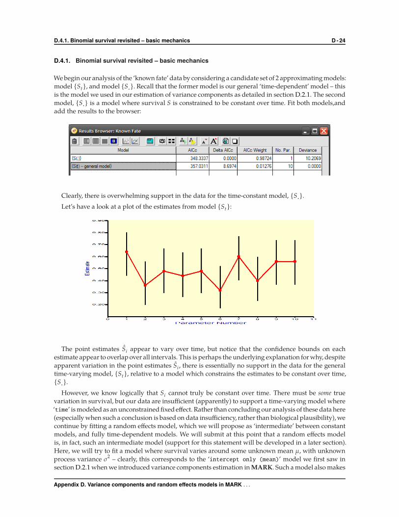
We begin our analysis of the ‘known fate’ data by considering a candidate set of 2 approximating models:
model {St}, and model {S·}. Recall that the former model is our general ‘time-dependent’ model – this
is the model we used in our estimation of variance components as detailed in section D.2.1. The second
model, {S·} is a model where survival S is constrained to be constant over time. Fit both models,and
add the results to the browser:
Clearly, there is overwhelming support in the data for the time-constant model, {S·}.Let’s have a look at a plot of the estimates from model {St}:
The point estimates Si appear to vary over time, but notice that the confidence bounds on each
estimate appear to overlap over all intervals. This is perhaps the underlying explanation for why, despite
apparent variation in the point estimates Si , there is essentially no support in the data for the general
time-varying model, {St}, relative to a model which constrains the estimates to be constant over time,
{S·}.However, we know logically that Si cannot truly be constant over time. There must be some true
variation in survival, but our data are insufficient (apparently) to support a time-varying model where
‘time’ is modeled as an unconstrained fixed effect. Rather than concluding our analysis of these data here
(especially when such a conclusion is based on data insufficiency, rather than biological plausibility), we
continue by fitting a random effects model, which we will propose as ‘intermediate’ between constant
models, and fully time-dependent models. We will submit at this point that a random effects model
is, in fact, such an intermediate model (support for this statement will be developed in a later section).
Here, we will try to fit a model where survival varies around some unknown mean µ, with unknown
process variance σ2 – clearly, this corresponds to the ‘intercept only (mean)’ model we first saw in
section D.2.1 when we introduced variance components estimation in MARK. Such a model also makes
Appendix D. Variance components and random effects models in MARK . . .
D.4.1. Binomial survival revisited – basic mechanics D - 25
some intuitive sense, if our intuition is guided by the time-series plot of the estimate Si shown on the
previous page, where it might be reasonable to ‘imagine’ each Si as ‘bouncing randomly’ around some
mean survival probability, µ (with the magnitude of the ‘bouncing’ around the mean being determined
by the process variance, σ2).
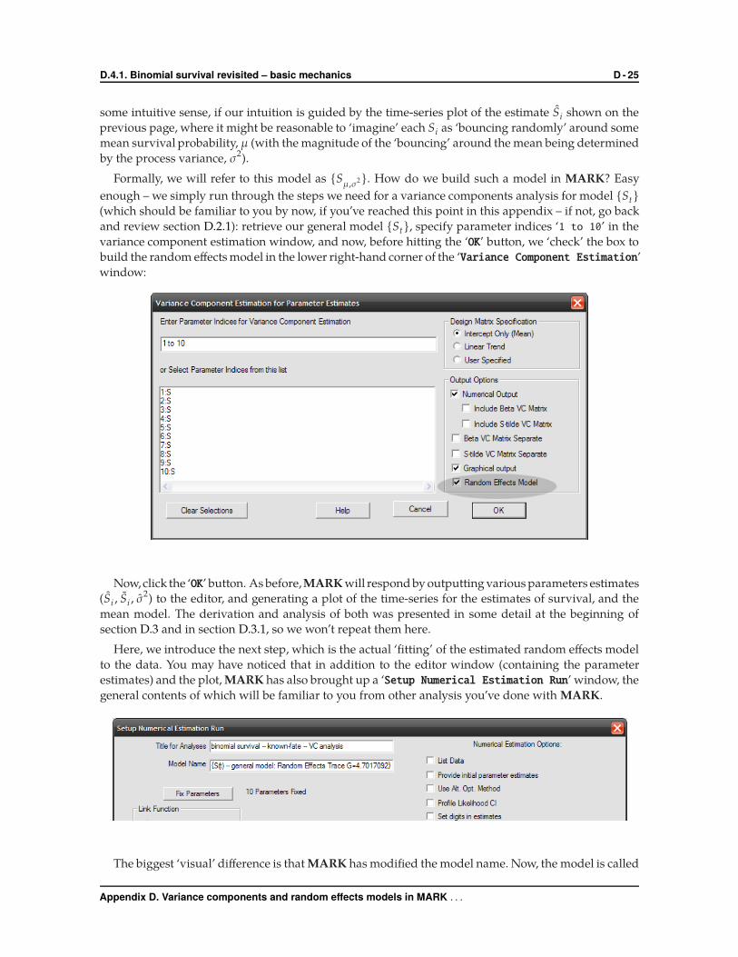
Formally, we will refer to this model as {Sµ,σ2}. How do we build such a model in MARK? Easy
enough – we simply run through the steps we need for a variance components analysis for model {St}(which should be familiar to you by now, if you’ve reached this point in this appendix – if not, go back
and review section D.2.1): retrieve our general model {St}, specify parameter indices ‘1 to 10’ in the
variance component estimation window, and now, before hitting the ‘OK’ button, we ‘check’ the box to
build the random effects model in the lower right-hand corner of the ‘Variance Component Estimation’
window:
Now,click the ‘OK’ button. As before,MARK will respond by outputting various parameters estimates
(Si , Si , σ2) to the editor, and generating a plot of the time-series for the estimates of survival, and the
mean model. The derivation and analysis of both was presented in some detail at the beginning of
section D.3 and in section D.3.1, so we won’t repeat them here.
Here, we introduce the next step, which is the actual ‘fitting’ of the estimated random effects model
to the data. You may have noticed that in addition to the editor window (containing the parameter
estimates) and the plot, MARK has also brought up a ‘Setup Numerical Estimation Run’ window, the
general contents of which will be familiar to you from other analysis you’ve done with MARK.
The biggest ‘visual’ difference is that MARK has modified the model name. Now, the model is called
Appendix D. Variance components and random effects models in MARK . . .

D.4.1. Binomial survival revisited – basic mechanics D - 26
‘{S(t)f(t) -- sin link: Random Effects Trace G=4.7017092}’. The part of the model name to the
left of the colon is what we originally used to name the model. The part to the right (which MARK has
added) indicates that we’re now running a random effects model, and that the ‘trace’ of the G matrix is
4.7017092. Recall from section D.3.2 that the trace of the G matrix is a related to the number of estimated
parameters used in the derivation of the AIC (and that because tr(G) is generally non-integer, that the
number of estimated parameters for random effects models is also usually non-integer). We’ll modify
the title by adding the words ‘intercept only (mean)’ somewhere in the title box, to indicate that the
model we’re fitting is the ‘intercept only (mean)’ model. Once done, click the ’OK to run’ button
and add the results to the browser (if you get a warning about MARK not being able to import the
variance-covariance matrix, ignore it).
Several things to note here. First, our random effects model now has some significant support in the
data (AICc weight is 0.383). While not the most parsimonious model in the candidate set, it is clearly
better supported than the fixed effect time-dependent model. However, given that a time-invariant
model is not logically plausible, then we should select a model where survival varies over time. If we
make such a logical choice, then (based on the ideas present in section D.3) our best estimate for annual
survival Si would be the shrinkage estimates Si from our random effects model, {Sµ,σ2}.
Second, look at the number of parameters that MARK reports as having beenestimated for this model
(4.70171). We see that this number is identical to tr(G). Recall from section D.3.3 that the dimension of
the parameter space (analogous to the number of estimated parameters in the usual sense) to associate
with a random effects model is Kre ,
Kre � tr(G) + ℓ,
where tr(G) is the trace of the G matrix, and ℓ is the number of free parameters not being modeled as a
random effect. In this case, all 10 parameters in the model, S1, . . . , S10 are being modeled as a random
effect, so ℓ � 0, and thus Kre � tr(G) � 4.70171.
If we next look at the estimates of Si (below)
we see that all of the estimates are ‘fixed’ at the value of Si . As fixed parameters in the fitted model,
Appendix D. Variance components and random effects models in MARK . . .

D.4.2. A more complex example – California mallard recovery data D - 27
there is no standard error (or CI) estimated (since there is nothing to be estimated for a fixed parameter,
obviously).
Finally, if you click on the ‘model notes’ button in the browser toolbar
you will be presented with a ‘copy’ of the variance components analysis which was first output to the
editor.
This is convenient, since it allows you to ‘store’ the variance components analysis for any particular
random effects model you fit to the data (note that the variance components analysis is output to the
‘model notes’ only if you run the random effects model).
D.4.2. A more complex example – California mallard recovery data
Here we introduce the mechanics, and some of the challenges, of fitting of ‘random effects’ models in
MARK. We will use a long-term dead recovery data set based on late summer banding of adult male
mallards (Anas platyrhynchos), banded in California every year from 1955 to 1996 (k � 41) (Franklin et
al., 2002). The total number of birds banded (marked and released alive) was 42,015, with a total of 7,647
dead recoveries. In a preliminary analysis, the variance inflation factor was estimated as c � 1.1952.
The recovery data are contained in california-male-mallard.inp. For your convenience, we’ve also
generated 3 candidate models: {St ft }, {ST ft }, and {S· ft}, where the capital ‘T’ subscript is used to
indicate linear trend. These models are contained in the associated .dbf and .fpt files.
Note that we use time-structure for the recovery parameter f . We do so not simply because such a
model often makes more ‘biological sense’ than a model where f is constrained (say, f·), but because
any constraint applied to f will impart (or ‘transfer’) more of the variation in the data to the survival
parameter S, such that the estimated process variance σ2 will be ‘inflated’, relative to the true process
variance. In general, you want to estimate variance components using a fully time-dependent model,
for all parameters, even if such a model is not the most parsimonious given the data.
Appendix D. Variance components and random effects models in MARK . . .

D.4.2. A more complex example – California mallard recovery data D - 28
Here are the results of fitting these 3 models to the data:
Based on the relative degree of support in the data it would seem that there is essentially no support
for a model where survival is constrained to follow a linear trend, or for a model where survival is
constrained to be constant over time. All of the support in the data (among these 3 models) is for model
{St ft }. If this was all we did, we’d come to the relatively uninteresting and uninformative conclusion
that there is temporal variation in survival. A plot of the estimates from this model seems to be consistent
with this conclusion:
However, rather than concluding our analysis of these data here, or perhaps add some models where
annual variation is modeled using a fixed effects approach where annual estimates are constrained to be
linear functions of one or more covariates, we might consider models which are ‘intermediate’ between
constant models, and fully time-dependent models. We will submit that a random effects model is, in
fact, such an intermediate model.
Let’s try to fit a model where survival varies around some unknown mean µ, with unknown process
variance σ2 – clearly, this corresponds to the ‘intercept only (mean)’ model. As was the case in our
first example involving binomial ‘known fate’ survival,we will refer to this model as {Sµ,σ2 ft}. Go ahead
and set up this model, first making sure that the fully time-dependent model is the ‘active’ model (by
retrieving it). Specify parameter indices ‘1 to 41’ for the variance component estimation, make sure
‘intercept only (mean)’ is selected, and that the ‘random effects model’ button is checked (as shown
at the top of the next page).
Appendix D. Variance components and random effects models in MARK . . .

D.4.2. A more complex example – California mallard recovery data D - 29
When you click the ‘OK’ button, you’ll be presented with the estimates of the mean, the ML and
‘shrinkage’ estimates, and the various estimates of the process variance (to save some space, we’ve
snipped out a number of the estimates for Si).
Appendix D. Variance components and random effects models in MARK . . .

D.4.2. A more complex example – California mallard recovery data D - 30
A plot of the ML and shrinkage estimates, and the model from which the shrinkage estimates were
derived (in this case, the intercept only mean model), is shown below:
Finally, we come to the estimation run window.
Again, we notice that MARK has modified the model name. Now, the model is called‘{S(t)f(t) --
sin link: Random Effects Trace G=32.0229017}’. The part of the model name to the left of the colon
is what we originally used to name the model. The part to the right (which MARK has added) indicates
that we’re now running a random effects model, and that the ‘trace’ of the G matrix is 32.0229. Again,
we’re going to modify the title slightly, to indicate that the model we’re going to fit is the ‘intercept
only (mean)’ model – we’ll simply add the words ‘intercept only’ somewhere in the title box.
Appendix D. Variance components and random effects models in MARK . . .

D.4.2. A more complex example – California mallard recovery data D - 31
We hit the ‘Ok to run’ button and...
Clearly, something has gone wrong. Generally when you see the phrase ‘numerical convergence
never reached’ (or something to that effect) embedded in an error message, your first response should
be to consider trying ‘better’ starting values. Often, such convergence issues reflect some underlying
‘problems’ with the data (sparseness, one or more parameters estimated near either 0 or 1), and MARK
is potentially having difficulty estimating the likelihood – a problem which might be exacerbated (or
simply an artifact) of the default starting values used in the numerical optimization.
One straightforward approach is to use different starting values – in this case, the ML estimates
from model {St ft }. To do this, simply check the ‘provide initial parameter estimates’ box in the
numerical estimation run window, before running the random effects model. Now, when you click ‘OK
to run’, you will be presented with a window asking you to specify the initial parameter estimates for
the numerical estimation. To use the estimates from model {St ft }, simply click the ‘retrieve’ button,
and select the appropriate model (labeled ‘S(t)f(t) -- sin link’). This will populate the boxes in the
‘initial values’ windows with the ML estimates. Then, once you click the ‘OK’ button, MARK will
attempt the numerical optimization. For this example, using these different starting values solves the
problem – the random effects model converges successfully.
An alternative approach which also generally works (albeit at the expense of some extended computa-
tional time in many cases), and which does not require good starting values for the optimization (which
you may not always have), is to use simulated annealing for the numerical optimization. You may recall
(from Chapter 10) that you can specify using simulated annealing for the optimization by selecting
the ‘alternate optimization’ checkbox on the right-hand side of the ‘run numerical estimation’
window. What simulated annealing does during the optimization is to periodically make a random
jump to a new parameter value. It is this characteristic is what allows the algorithm more flexibility in
finding the global maximum (in cases where there may in fact by local maxima in the likelihood; see
Chapter 10 for a discussion of this in the context of multi-state models), and minimizes the chances that
the numerical solution is determined by starting values (simulated annealing starts with the defaults,
but then makes the random jumps around the parameter space, as described).
To use simulated annealing for our mallard analysis, you simply retrieve model {St ft} (our general
model), run through the variance components analysis (remembering to check the ‘random effects
model’ box), and then try again – this time, before hitting the ‘OK to run’ button for the generated
random effects model, make sure the ‘Use Alt. Opt. Method’ button is checked. Change the title (we’ll
add ‘intercept only model -- SA’ to indicate both the model, and the optimization method used
to maximize the likelihood), then click ’OK to run’. Simulated annealing takes significantly longer to
converge than does the default optimization routine – how much longer will depend on how fast your
computer is. Nonetheless, this approach also works fine, and yields the same model fit as the model fit
using different initial values for the optimization. We’ll only keep one of these in the browser (shown
at the top of the next page).
Appendix D. Variance components and random effects models in MARK . . .

D.4.2. A more complex example – California mallard recovery data D - 32
We see that the ‘intercept only’ random effects model has virtually all the support in the data,
even relative to our previous ‘best model’ {St ft}. Again, we note that the number of parameters
estimated for the random effects model is non-integer. Note, however, that the number of parameters
estimated (74.02363) is not simply tr(G) (=32.02363). The difference between the two values is (74.02363-
32.02363)=42. Where does the 42 come from? Recall that the number of parameters estimated for the
random effects model, Kre is given as Kre � tr(G) + ℓ, where ℓ is the number of free parameters not
being modeled as a random effect. In our mallard example, we modeled the 41 survival parameters
S1, . . . , S41 as a random effect, but we left the recovery parameter f modeled over time as a simple fixed
effect. How many f parameters in our model? ℓ � 42, which of course is why the number of parameters
estimated is 42 more than tr(G).
What more can we about our results so far? Consider the improvement in precision achieved by the
shrinkage estimates, Si, from model {Sµ,σ ft } compared to the ML estimates, Si from model {St ft}. As
discussed in section D.3.2, a convenient basis for this comparison is the ratio of average �RMSE to SE:
�RMSE(Si
�� Si
)SE
(Si
�� Si
) �0.06476
0.07870� 0.823.
The average precision of the shrinkage estimates is improved, relative to MLEs,by 18%,hence confidence
intervals on Si would be on average 18% shorter.
Let’s continue by fitting a linear trend random effects model. First, retrieve model {St ft}. Then, start
a ‘variance components’ analysis – this time, selecting the ‘linear trend’ design matrix specification,
instead of the default ‘intercept only (mean)’. Here is a truncated listing of the numerical estimates.
Appendix D. Variance components and random effects models in MARK . . .

D.4.3. Random effects – environmental covariates D - 33
We see that the estimated process variance is nearly half the value estimated from the intercept only
model. We also see that the estimate for the slope is positive (β � 0.0034). This is reflected in the plot of
the ML and shrinkage estimates against the model, shown below:
Next, we’ll go ahead and fit the estimated ‘linear trend’ RE model to the data, after adding the
phrase ‘linear trend’ to the title.
Here is the results browser with the ‘linear trend’ random effects model results added:
We see clear evidence of strong support for random variation in the individual Si around the trend
line – this model has almost twice the support in the data as the next best model (our intercept only
model). What is of particular note is that if we hadn’t built the random effects models, and had based our
inference solely on the 3 starting models, we would have concluded there was no evidence whatsoever
of a trend, when in fact, the random effects trend model ended up being the best supported by the data.
The simple random effects models we used here are both necessary for inference about process
variation, σ2, and also for improved inferences about time-varying survival rates.
D.4.3. Random effects – environmental covariates
Here, we consider fitting a random effects model when survival differs as a function of some envi-
ronmental covariate. Suppose we have some live encounter (CJS) data collected on a fish population
studied in a river that is subject to differences in water level. You hypothesize that annual fish survival
is influenced by variation in water level. We have k � 21 occasions of mark-recapture data (contained
Appendix D. Variance components and random effects models in MARK . . .

D.4.3. Random effects – environmental covariates D - 34
in level-covar.inp). Over each of the 20 intervals between occasions, water flow was characterized as
either ‘average’ (A) or ‘low’ (L) (more specific covariate information was not available). Here is the time
series of flow covariates: {AAAALLLAAALALALLLLAL}.We begin our analysis by considering 3 fixed effect models for apparent survival, ϕ: {ϕt pt}, {ϕ· pt}
and {ϕleve l pt }. Here are the results from fitting these 3 models to the data:
We see strong evidence for variation over time in apparent survival, but no support for an effect of
water level. If you look at the estimates from model {ϕleve l} for average (ϕav g � 0.709, SE � 0.0106) and
low (ϕlow � 0.650, SE � 0.0100), the lack of any support for this model may not be surprising. At least,
based on considering water level as a fixed effect.
Now let’s consider some random effects models. We’ll build 2 different models – one a simple
intercept only (mean) model, which would seem to be consistent with the strong support for the simple
time variation model {ϕt}, and one where survival is thought to vary randomly around a level-specific
mean. In other words, we hypothesize µlow , µav g . We’ll assume, however, that σ2low � σ2
hi gh . This is
not directly testable using the moments-based variance components approach in MARK, but is testable
using an MCMC approach (see appendix E).
By this point, building and fitting the intercept only model for the survival parameters ϕ1 → ϕ19
(remember, we don’t include ϕ20 since it is confounded with our estimate of p21 for our time-dependent
model) should be straightforward,so we’ll skip the description of the mechanics,and will simply present
the results – we’ve added the ‘intercept only’ model to the browser (below).
We see strong evidence that the intercept only random effects model is more parsimonious given the
data than any other model.
Now, we consider the final model where survival is though to vary randomly around a level-specific
mean. We’ll refer to this as model {ϕµlevel σ
2level
}. How do we construct this model in MARK? Here
we finally make use of the ‘User Specified’ design matrix option in the variance components setup
window (shown at the top of the next page). Simply retrieve the time-specific fixed effect model {ϕt pt },start the variance components analysis, specify the parameters (1 to 20), and check the ‘User Specified’
design matrix option. Make sure you’ve also checked the ‘Random Effects Model’ option as well.
Appendix D. Variance components and random effects models in MARK . . .

D.4.3. Random effects – environmental covariates D - 35
Now, all we need to do is click the ‘OK’ button. Once you do so, MARK will present you with a small
pop-up window asking you to specify how many covariate columns you want in the user-specified
design matrix. The default is 3, but here, for our model, we need only 2: one to code for the intercept,
and one to code for the water level (a single column since there are only two levels of the water covariate).
The design matrix entry window is shown below:
Note that there are only 19 rows in the DM, since we’re applying a random effect to ϕ1 → ϕ19 only.
Also note the small ‘pop-up’ window indicating that ‘When you have filled out the design matrix,
click OK to continue’. Meaning you should do as it says – specify your design matrix for the survival
Appendix D. Variance components and random effects models in MARK . . .

D.4.3. Random effects – environmental covariates D - 36
parameters, and then when you’re sure it’s correct, click the ‘OK’ button.
First we’re presented with a plot (below), showing the ML and shrinkage estimates, and (importantly
here) the underlying model (the red line).
The red line clearly indicates that there are 2 separate means being modeled, for the low and average
water flow years, respectively. The estimated process variance is σ2� 0.00313, and the estimate for
β1 � 0.0717 in the linear model indicates that survival is higher in ‘average’ water level years (since we
used ‘low’ level years as the reference level in our design matrix, above). What is also very important
here, is that the shrinkage estimates are clearly not constrained to fall exactly ‘on the red line’ – they
represent shrunk estimates of apparent survival as if each estimate was drawn randomly from a sample
with a water level-specific mean.
OK, what about the results of fitting this random effects model to the data?
What is especially noteworthy here is that the random effects model with water level-specific means,
{ϕµlevel σ2level
}, is now the most parsimonious model in the model set, despite ‘water level’ having
no support whatsoever when considered in a fixed effects design. The near equivalence of the AICc
weights between this model and the simpler ‘intercept only’ random effects model suggest that we
can’t differentiate between the two, but whereas our initial conclusion strongly rejected the hypothesis
that there was an influence of water level on apparent survival, our random effects modeling would
suggest that perhaps we shouldn’t be quite so sure.
Appendix D. Variance components and random effects models in MARK . . .

D.4.4. Worked example – λ – Pradel model D - 37
D.4.4. Worked example – λ – Pradel model
We conclude with analysis of a famous set of data, the moth (Gonodontis bidenta) data reported on by
Bishop et al. (1978) and compulsively analyzed by many others (e.g., Link & Barker 2005). The data
consist of records for 689 male moths that were captured, marked, and released daily over 17 days in
northwest England. These moths were nonmelanic; demographic parameters were estimated as part of
a larger study looking at comparative fitness of distinct color morphs.∗
Here we will use random effect Pradel models (Chapter 13), focussing on estimation of process
variance, and possible trend, in realized growth rate λ. The data we’ll work with are contained in
moth-example.inp. Our focus here is on variation in λ. Recall that in a Pradel model, λ an be estimated
as either a structural (real) parameter (for data type ‘survival and lambda’), or as a derived parameter
(for any of the other Pradel model data types). For the purposes of estimating process variance on λ, it
doesn’t particularly matter which data type we use, since we can estimate process variance for either
real or derived parameters. We have already seen variance components analysis of real parameters in
earlier examples, so here, we’ll demonstrate the process of estimation for λ as a derived parameter.
To start, select the data type ‘Pradel survival and seniority’. 17 occasions. Now, you may recall
that there are some challenges with parameter confounding for fully time-dependent Pradel models.
As is often the case, some of these problems can be handled by applying constraints to one or more
parameters. Since our purpose here is simply to demonstrate some mechanics, and not conduct an
exhaustive analysis of these data, we’ll avoid some of these issues by simply setting the encounter
probability p to be constant over time. So, our general model will be {ϕt p· γt }. Go ahead and modify
the PIM chart to construct this model, and add the results to the browser. Model deviance is 236.708.
Here are the derived estimates
Note that MARK generates derived estimates of λ, and log λ. While there are important considera-
tions as to which is more appropriate for analysis (see discussion in Chapter 13), our purpose here is
∗ The underlying motivation for this study should be very familiar to any of you with some background in evolutionary biology.
Appendix D. Variance components and random effects models in MARK . . .

D.4.4. Worked example – λ – Pradel model D - 38
simply to demonstrate some of the ‘mechanics’, so we’ll focus on estimates of λ on the linear scale.
Let’s construct a random effects model for λ, using {ϕt p· γt } as our general model. The steps are the
same, except that when you access the ‘variance components’ sub-menu, you need to specify ‘derived
parameter estimates’ for the parameter type. You’ll be asked to select either ‘Lambda Population
Change’ or ‘log(Lambda) Population Change’. We’ll select the former.
Now, for the first ‘challenge’ – specifying the parameter index values for λ. You might simply assume
that you would select all of them: 1 to 16. However, here (and generally), we need to be a bit careful.
When specifying the parameters to include in the random effect, you should not include parameters
that are confounded, or that are otherwise known to have ‘issues’. For Pradel models, there is potential
for confounding, but constraining encounter probability p to be constant over time should solve some
of that problem. However, experience has shown that the first and last estimates of λ in Pradel models
are often biased. If you look at the estimates for λ1 and λ16 shown on the previous page, you’ll see some
evidence that this might be the case for these data. For example, λ1 � 3.217. This is often a judgement
call (for example, you might say that λ11 � 3.55 is even larger, so using scale as evidence for a ‘problem’
with λ1 is perhaps not a great criterion). For now, we’ll be ‘conservative’, and include only λ2 → λ15 in
specifying the random effect.
Now, for one important difference in fitting random effects models to derived parameters – you can’t.
If you look in the lower-right-hand corner, you’ll notice that the ‘Random Effects Model’ check-box has
been ‘greyed-out’.
If you think about it, this should make some sense. The random effects ‘constraint’ can be applied
only to real (structural) parameters in the model. Here, we are estimating λ as a derived parameter
(i.e., by algebra), and thus we can’t build and fit a random effects model using the Pradel ‘Survival and
seniority only’ data type. We’ll revisit this point in a moment. Go ahead and click the ‘OK’ button. The
plotof the real estimates λi andshrinkage estimates λi is shown at the top of the nextpage. The estimated
mean ¯λ � 1.147, with an estimated process variance of σ2� 0.722. The plot shows clear evidence of
fairly large swings in realized growth – this is not overly surprising for an insect, where large changes
in reproduction and survival are relatively commonplace (there aren’t enough data available to test for
‘boom-bust’ cycles, another common occurrence with insect growth dynamics).
Now, what if we wanted to fit a random effects model for λ, and not simply estimate the mean and
process variance? To do this, we need to change the data type, to one where λ is included as a structural
Appendix D. Variance components and random effects models in MARK . . .
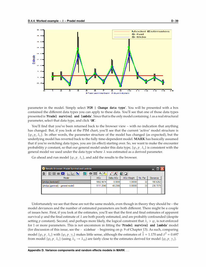
D.4.4. Worked example – λ – Pradel model D - 39
parameter in the model. Simply select ‘PIM | Change data type’. You will be presented with a box
contained the different data types you can apply to these data. You’ll see that one of those data types
presented is ‘Pradel survival and lambda’. Since that is the only model containingλ as a real structural
parameter, select that data type, and click ‘OK’.
You’ll find that you’ve been returned back to the browser view – with no indication that anything
has changed. But, if you look at the PIM chart, you’ll see that the current ‘active’ model structure is
{ϕt pt λt }. In other words, the parameter structure of the model has changed (as expected), but the
underlying model has reverted back to the fully time-dependent model. MARK has basically assumed
that if you’re switching data types, you are (in effect) starting over. So, we want to make the encounter
probability p constant, so that our general model under this data type, {ϕt p· λt } is consistent with the
general model we used under the data type where λ was estimated as a derived parameter.
Go ahead and run model {ϕt p· λt }, and add the results to the browser.
Unfortunately we see that these are not the same models, even though in theory they should be – the
model deviances and the number of estimated parameters are both different. There might be a couple
of issues here. First, if you look at the estimates, you’ll see that the first and final estimates of apparent
survival ϕ and the final estimate of λ are both poorly estimated, and are probably confounded (despite
setting p constant). Second, and perhaps more likely, the logical constraint that λi > ϕi is not enforced
for 1 or more parameters. This is not uncommon in fitting the ‘Pradel survival and lambda’ model
(for discussion of this issue, see the - sidebar - beginning on p. 9 of Chapter 13). As such, comparing
model {ϕt p· λt } with {ϕt p· γt } makes little sense, although the estimates of ¯λ � 1.170 and σ2� 0.697
from model {ϕt p· λt } (using λ2 → λ15) are fairly close to the estimates derived for model {ϕt p· γt }.
Appendix D. Variance components and random effects models in MARK . . .

D.5. Model averaging? D - 40
For the moment, we’ll skip over this issue, and focus on some additional ‘mechanics’. Delete model
{ϕt p· γt } from the browser – we’ll focus on model {ϕt p· λt }. We are interested in analysis of trend in
λ. Trend in realized λ is potentially of great significance for conservation and management, and robust
estimation of trend would seem to be something worth pursing. Now, based on the plot of λi and λi
shown at the top of the preceding page, we don’t expect a ‘trend’ model of any flavor to have much
support in the data. But, to demonstrate the mechanics, we’ll proceed anyway.
With model {ϕt p· λt }, we can see there are at least 2 ways we could proceed. We could build an
ultrastructural model where λ is constrained to fall on a straight trend line, or we could build a random
effects trend model. We’ll do both, for purposes of comparison. To make the comparison ‘fair’, we’ll
build the ‘T’ (trend) ultrastructural model applied to λ2 → λ15 only, since these are the parameters we
would use in the random effects model. Then, we’ll build the random effects ‘trend’ model, also using
λ2 → λ15 only, and add the results of both to the browser.
We notice immediately that the random effects modelwith trendactually gets a fairamountof support
in the data, especially relative to the ultrastructural fixed effects trend model. So, despite appearances,
there might be some evidence of trend in the data. Enough that the overall support for this model is
fairly compelling.
At least 2 points to make here. First, there are some general concerns with the ultrastructure approach,
where constraints are applied to λ. Since growth is a function of per capita survival plus per capita
recruitment, λ � ϕ + f , then any constraint applied to λ enforces a strict negative covariance between
ϕ and f (see chapter 13, and discussions in Franklin 2001). Such a covariance is clearly artificial, and
may make little to no biological sense (since it would imply that any increase in survival is perfectly
balanced by an equal and opposite change in recruitment). Second, the random effects approach to
trend analysis can’t be applied to λ when λ is estimated as a derived parameter – you can estimate the
intercept and slope of the trend, and the process variance, but you can’t fit a random effects model for
a derived parameter (i.e., you cannot add it to the browser).
While there are some technical challenges withPradelmodels in general (especially for time-dependent
models,whichare exacerbated forrandom effects models whichare generally applied to time-dependent
models), it seems clear that considering variance components and random effects analysis forλ in Pradel
models has potential to be extremely useful.
D.5. Model averaging?
At this point, you might be asking yourself, ‘what about model averaging?’. This important topic is
introduced in some detail in Chapter 4 (see the Burnham & Anderson ‘model selection’ book for a
comprehensive treatment).
There are at least two issues to consider here. First, if our candidate model set contains both fixed
effect and random effect models, should we model average over the entire set? In fact, MARK does
nothing ‘mechanically’ to prevent you from doing so. For example, take the mallard analysis intro-
Appendix D. Variance components and random effects models in MARK . . .

D.5. Model averaging? D - 41
duced in section D.4.2. Assume that we have the following 5 models in the browser – 3 fixed effects
models ({St ft }, {S· ft }, {ST ft }), and 2 random effect models (‘linear trend model’, and ‘intercept
only (mean) model’:
You can go ahead and run the model averaging routines on the survival estimates – MARK simply
assumes you want to average over the entire model set. Your only hint that you might need to be a bit
careful comes when you look at the model averaging output. Here is a snippet of the output for the
mallard analysis, for the parameter corresponding to S1:
Pay particular attention to the right-hand side. Notice that for the 2 random effects models, you get a
‘warning’ about ‘invalid parameter estimates’ with ‘zero SE?’. MARK has ‘noticed’ that the parameter
estimates for parameters modeled as random effects (the survival parameters, in this case) have a zero
SE. MARK ‘suspects’ there might be a problem, but in fact this is exactly what you should see. As
discussed earlier, the random effects model is fit to the data after fixing the random parameters to
their shrinkage estimates, and thus, there is no SE for those parameters. And, since model averaging
intends to generate an unconditional parameter estimate, by accounting for conditional uncertainty
in the parameter for each model, then there are clear problems when one or more of the parameters
‘appear’ to be estimated without any uncertainty (i.e., have zero SE’s). So, if MARK included the random
effect parameter estimates in the model averaging, then the estimate of the unconditional SE for that
parameter would be very negatively biased (i.e., much too small).
The second issue is ‘conceptual’, and relates broadly to the issue of ‘model redundancy’. In the
extreme, having 2 structurally identical models in the same candidate model set would clearly render
model averaged estimates invalid. Model redundancy in the context of AIC selection is discussed in
Burnham and Anderson (sections 4.2.9 and 4.2.10). With some thought, you might see that the random
effects model is substantially redundant to its fixed effects likelihood version. For example, model
{Sµ,σ ft } would be redundant to some degree to model {St ft}.In one sense, a random effects model is a model which is intermediate between a time-invariant
(‘dot’, say S·) model, and a fully time-varying fixed effects model (say, St). Recall from section D.3 that
Appendix D. Variance components and random effects models in MARK . . .

D.6. Caveats, warnings, and general recommendations D - 42
shrinkage estimates Si generally lie between E(S) and Si . Recall from section D.3.1 that in the absence
of sampling covariance, the shrinkage estimator used in MARK is
Si � E(S) +
√√√√ σ2
σ2+ ES
[var
(Si
�� Si
) ] ×[Si − E(S)
].
Consider the estimates of survival for the first interval from the binomial example presented in section
D.2.1: the ML estimate S1 � 0.640, the mean survival E(S) � 0.484, and the shrunk estimate S1 � 0.548.
As shown in the following
E(S) S1 S1
0.484 0.548 0.640
‘shrunk toward the mean’
the ML estimate is ‘shrunk’ toward the mean, with the resulting shrinkage estimate, S1 being ‘inter-
mediate’ between the mean, E(S) (which is equivalent to a ‘dot’ model, in some respects) and the ML
estimate S1 (which comes from the ‘time-dependent’ model). So, the shrinkage estimate is analogous to
an ‘average’ between the two estimates. As noted in section D.3, the degree of shrinkage is determined
by the magnitude of the process variance σ2, relative to the sampling variance, ES[var(Si
�� Si
)]. If the
process variance is relatively small, then the shrunk estimates will approach the estimate for the mean
E(S),whereas if the process variance is large relative to the sampling variance, then the shrunk estimates
will be closer to the ML estimates, Si. So, the shrinkage model {Sµ,σ , θ}, is intermediate between model
{St , θ} and model {S· , θ}, and is thus strongly analogous to an ‘average model’. As a result, when the
process and sampling variances are similar, the estimates from model {Sµ,σ , θ} will tend to be quite
similar to the model-averaged estimates estimated over model {St , θ} and model {S·, θ}.
D.6. Caveats, warnings, and general recommendations
Using random effects as a basis for modeling collections of related parameters is a long-standing
approach in statistics and one that can be very effective. Use of the random effects approach in capture-
recapture is relatively new – in the nearly 10 years since the publication of B&W, there have been
relatively few applications of these models to real data, despite what we believe are several interesting
opportunities made available by these methods.
However, we also believe that the methodology needs to be better understood as to any potential
pitfalls and as to its operating characteristics. The following is a summary of our experience to date
with random effects models, particularly as implemented in MARK. This material is largely abstracted
from B&W, and accumulated experience with such models since the time of that publication.
1. the ‘method of moments’ described in the appendix, and as implemented in MARK, has
been shown to perform well, especially when σ2 > 0.025. The method(s) may not do so well
if σ2 → 0. However, we think it reasonable to believe that for a worthwhile study yielding
good data,process variation,σ2,will generally not be too small, relative to average sampling
variation and it is for these conditions (of ‘good data’) that we need effective random effects
inference methods.
Appendix D. Variance components and random effects models in MARK . . .

D.6. Caveats, warnings, and general recommendations D - 43
2. Another issue to be aware of, as regards estimation of the parameter σ2, is the matter
of unequal, rather than equal length, time intervals. Let the time interval i have length
∆i . Then we should parameterize the model as Si � (ψi)1/∆i where now each survival
probability ψi is on the same unit time basis. It may then make biological sense to consider
parameters that are a mean and variation forψ1, . . . , ψk . But this may just as well not make
sense, because the time intervals are intrinsically not comparable as they may be in very
different times of the annual cycle. It becomes a subject matter judgement as to whether
random effects analysis will be meaningful with unequal time intervals. For the moment,
don’t apply random effects models or variance components analysis to situations where
the intervals between sampling occasions are unequal (even specifying unequal interval
length will generally yield negatively biased estimates of process variance, σ2).
3. In practice if there is over-dispersion in the data, as measured by a scalar often denoted
by c (see Chapter 4 and Chapter 5), the estimated sampling variance-covariance must be
adjusted by a reliable c (see discussion in B&W, and Franklin et al. 2002 for an example
with real data).
4. A key design feature to focus on to meet the criterion of ‘having good data’ when applying
random effects is k, the number of estimable random effects parameters (time intervals,
locations, etc.). The sample size for estimating σ2 is k. Therefore, one must not have k too
small; < 10 is too small. Even if we knew all the underlying Si a sample of size k < 10 is too
small for reliable inference about the variation of these parameters (even given a random
sample of them, which is not required here). Inference performance has been shown to
be acceptable when k > 15. The benefits (includes shrinkage estimates) of random effects
models become greater as the number of underlying parameters, k, increases.
5. The other influential design feature is number of individuals marked and released. Both
numbers initially released and numbers recaptured are important to the performance of
inferences from random effects models. While there are no ‘hard and fast’ rules, we can
make some general recommendation. B&W showed that low numbers of marked and
released animals, especially for low survival and encounter probabilities, generally led to
point estimates of σ2 → 0 – this is because the sampling variation was much larger than
process variance in these cases.
6. The situation where inferences from a random effects model are most advantageous
seems to be for when σ2 is about the same as average sampling variance, (Si | Si) (recall
that sampling variance is strongly influenced by sample size of animals capture and
reencountered, whereas process variance is not). If one or the other variance component
dominates the total variation in the MLE’s Si then the data strongly favor either the simple
model {S· pt } (sample variance dominates), or the general model {St pt} (process variation
dominates), rather than the random effects model.
However, it is not a problem, as regards inference about σ2, to have large sample sizes
of animals, hence small sampling variances, so that should be one’s design goal. If it then
turns out that sampling variance is similar to process variance, the random effects model
will be markedly superior to model {St pt}. Thus, in a sense the random effects model is
optimal at the ‘intermediate’ sample size case. As sample size of animals increases, the
random effects model converges to model {St pt}.7. A potential technical issue is the ‘boundary effect’ (at least under what is basically a
likelihood approach). As discussed in B&W, if one enforces the constraint S < 1 when
the unbounded MLE S ≥ 1, then standard numerical methods used in MARK to get the
observed information matrix fails. As a result, the estimated information matrix is incorrect
for any terms concerning the S that is at the bound of 1 (and the inverse information
Appendix D. Variance components and random effects models in MARK . . .

D.7. Summary D - 44
matrix is likely wrong in all elements). Experience shows that, in this case, the resultant
point estimate of σ2 can be very different from what one gets when the survival parameter
MLE’s are allowed to be unbounded. The difference can be substantial. Using an identity
link, B&W found σ2 to be unbiased in many cases.∗ With good data we rarely observe an
unbounded MLE of S that exceeds 1. This might be explored in a Bayesian context, where
it is easy (in a MCMC analysis) to allow S to have its distribution over an interval such as 0
to 2 (rather than 0 to 1). B&W considered this, and found a strong effect of the upper-bound
on the point estimate (and entire posterior distribution) for σ2, and for that particular S.
(Note: MCMC applications in MARK are discussed in Appendix E).
D.7. Summary
This appendix has considered random effects models. The name ‘random effects’ can be misleading in
that a person may think it means that underlying years or areas (when spatial variation is considered,
rather than temporal) mustbe selectedat random.This is neither true,norpossible,fora setof contiguous
years. Variance components is a better name, in that at the heart of the method is the separation of
process and sampling variance components. The issue of what inferential meaning we can ascribe to σ2
is indeed tied to design and subject matter considerations. However, the shrinkage estimators do not
depend on any inferential interpretation of σ2; rather, they can always be considered as improvements,
in a MSE sense, over the MLEs based on full time-varying St . The random effects model only requires
that the residuals (Si − XB) are exchangeable.
When are we interested in these sorts of models? Often, if a data set is sparse, but with many (≥ 10)
occasions, model {S(.)} will be selected. Clearly, this is a model, as we know that conditional survival
probability cannot remain exactly the same over any significant length of time. While model {S(.)}might
be ‘best’ in the sense of a bias-variance trade-off (i.e., it is identified by AIC as most parsimonious among
the candidate models), it might leave the investigator wondering about the variation in the parameters.
Thus, the estimation of σ2 has relevance. At the other extreme, assume that model {St} is selected; here
the investigator might have (say) 25 estimates of the survival parameters, each perhaps with substantial
sampling variation. This makes it difficult to see patterns (e.g., time trends orassociations) orunderstand
the variation in the parameters. Further, analysis of stochastic population models is often complicated
by uncertainty concerning the relative variation in estimates of one or more demographic parameters.
Random effects models are a very interesting class of models which can address both issues (amongst
many more), but even a partial understanding is somewhat difficult to achieve. The intent of this
appendix was to try to convey the general notion of random effects models, and the idea of ‘variance
components’, as implemented in program MARK, in a reasonably accessible fashion. The subject of
random effects models and variance components as applied to data from marked individuals is treated
in considerably more depth in several of the following papers. An alternative approach to estimating
variance components, based on Bayesian inference (sensu Royle and Link, 2002) and Markov Chain
Monte Carlo (MCMC), is presented in Appendix E.
∗ Note that we do not suggest routinely accepting final inferences that include survivalestimates exceeding 1. In fact, the shrinkage
estimates will generally not exceed 1, so using Si and not Si will be the needed improved inference. However, to get to thisfinal inference it may be desirable to pass through an imaginary space (S > 1), just as imaginary numbers can facilitate realsolutions to real problems. Models only need to possess utility, not full reality.
Appendix D. Variance components and random effects models in MARK . . .
D.8. References D - 45
D.8. References
Burnham, K. P., Anderson, D. R., White, G. C., Brownie, C., and Pollock, K. H. (1987) Design and Analysis
Methods for Fish Survival Experiments Based on Release-Recapture. American Fisheries Society Mono-
graph No. 5. Bethesda, Maryland, USA. 437 pp.
Burnham, K. P., and White, G. C. (2002) Evaluation of some random effects methodology applicable to
bird ringing data. Journal of Applied Statistics, 29, 245-264.
Efron, B., and Morris, D. (1975) Data analysis using Stein’s Estimator and its generalizations. Journal of
the American Statistical Association, 70, 311-319.
Efron, B., and Morris, D. (1977) Stein’s paradox in statistics. Scientific American, 238, 119-127.
Franklin, A. B., Anderson, D. R., and Burnham, K. P. (2002) Estimation of long-term trends and variation
in avian survival probabilities using random effects models. Journal of Applied Statistics, 29, 267-287.
Gould, W. R., and Nichols, J. D. (1998) Estimation of temporal variability of survival in animal popula-
tions. Ecology, 79, 2531-2538.
Pfister, C. A. (1998) Patterns of variance in stage-structured populations: evolutionary predictions and
ecological implications. Proceedings of National Academy of Science, 95, 213-218.
Royle, J. A.,andLink,W. A. (2002) Random effects andshrinkage estimation in capture-recapture models.
Journal of Applied Statistics, 29, 329-351.
Schmutz, J. A. (2009) Stochastic variation in avian survival rates: life-history predictions, population
consequences, and the potential responses to human perturbations and climate change. Pages 441-
461 in D. L. Thomson, E. G. Cooch, and M. J. Conroy, editors. Modeling Demographic Processes in
Marked Populations. Springer, Berlin.
White, G. C. (2000) Population viability analysis: data requirements and essential analyses. Pages 288-
331 in L. Boitani and T. K. Fuller, editors. Research Techniques in Animal Ecology: Controversies and
Consequences. Columbia University Press, New York, New York, USA.
White, G. C., Burnham, K. P., and Anderson, D. R. (2001) Advanced features of Program MARK. Pages
368-377 in R. Field, R. J. Warren, H. Okarma, and P. R. Sievert, editors. Wildlife, Land, and People: Pri-
orities for the 21st Century. Proceedings of the Second International Wildlife Management Congress.
The Wildlife Society, Bethesda, Maryland, USA.
White, G. C. 2000. Population viability analysis: data requirements and essential analyses. Pages 288-
331 in L. Boitani and T. K. Fuller, editors. Research Techniques in Animal Ecology: Controversies and
Consequences. Columbia University Press, New York, New York, USA.
Appendix D. Variance components and random effects models in MARK . . .