appendix d - transform 66 in northern virginia - outside the...
TRANSCRIPT

Tier 2 Final Environmental Assessment I-66 Existing Conditions Report
Appendix DVISSIM Calibration Assumptions Memorandum
FINAL – MAY 2016
I-66 Consultant Team 1 Microsimulation Assumptions and Calibration Results (DRAFT)
MEMORANDUM
To: Randy Dittberner, P.E., PTOE/VDOTRobert Josef/VDOT
From: I-66 Traffic Operations Team
Date: August 10, 2015
Subject: I-66 TTR/IJR VISSIM Calibration Assumptions, Methodology, and Results
INTRODUCTIONAs part of the traffic analyses needed for the development of the Interchange Justification Report (IJR)and the Transportation Technical Report (TTR) for the I-66 Corridor Improvements Project, the Kimley-Horn (KH) and CH2M HILL (CH) I-66 TTR/IJR project team conducted calibration of VISSIM trafficsimulation models developed for the 2014 Existing Conditions for both AM and PM peak periods andportions of the AM and PM shoulder periods. This memorandum provides a detailed description ofassumptions and methodologies employed for the calibration as well as the summary of calibrationresults. In addition, the memorandum describes the methodology used for the estimate of vehiculardemand and routing data for the entire network.
Characteristics of the I-66 Corridor Microsimulation Efforts
The analysis network for the I-66 corridor microsimulation is larger and more complex than thenetworks for most simulation efforts. The key variables for a simulation are the number of vehicles, thesize of the network (number of links and/or intersections), the level of congestion, and the duration ofthe analysis period. The I-66 corridor microsimulation study is more complex on most of thesemeasures, especially for the level of congestion (10-12 hours a day in several parts of the corridor) andhigh freeway traffic volumes. A sample of mainline I-66 data is presented in Figure 1 and Figure 2,representing the average weekday hourly volumes at the beginning, middle, and end points of the I-66corridor. As shown in Figure 1, the diurnal curves indicate the expected distribution of volume during anaverage weekday in the eastbound direction, with the highest volumes observed during the AM peakperiod. It is also noted that the highest daily volume occurs at the eastern limits of the I-66 corridor inthe more densely populated areas where higher hourly volumes are sustained throughout the day. Theopposite is true at the western limits of the corridor. In Figure 2, less defined travel patterns areobserved in the westbound direction. At the western limits of the I-66 corridor, hourly volumes peak
I-66 Consultant Team 2 Microsimulation Assumptions and Calibration Results (DRAFT)
during the late afternoon hours between 3:00 p.m. and 5:00 p.m. A similar pattern is observed betweenRoute 28 and US 29; however, in the westbound direction between I-495 and Route 243, hourly volumespeak twice, with the AM peak volume being comparable to the late evening volume, and two peaks involume occur at 2:00 p.m. and again at 7:00 p.m., indicating a larger spread in the peak-period volumescompared to the other two locations downstream.
The review of INRIX data collected between June 2013 and May 2014 indicated a significant reduction inaverage mainline I-66 travel speeds at key points along the study corridor. This can be attributed toincreased congestion and volume associated with peak travel. The greatest duration of reduced travelspeeds was noted in the eastbound direction at the US 50 interchange between approximately 6:00 a.m.and 10:30 a.m. and in the westbound direction at the Route 243 interchange between approximately1:30 p.m. and 8:30 p.m. Both interchanges are located at the eastern limits of the study corridor wherehigher daily volumes are observed.
One of the early findings from the data collection and field observations was the fact that a single peakhour for the entire system does not exist. The peaking patterns along the corridor vary significantlyduring the peak period in terms of absolute peak volume, location, and duration. Furthermore, lane useand vehicle restrictions vary along the corridor during the analysis hours (e.g., HOV restriction inside oroutside the Beltway and shoulder lane use during several hours and in the direction of the peak flow). Asa result, a multi-hour analysis including the peak period, but extending beyond the peak period toinclude the shoulders of the peak, was required for the analysis.
The focus of the project is to improve freeway operations during the peak periods. While there ismidday congestion in some locations in the corridor, the analysis has been focused on the peak periodsand the hours before and after the peak period where lane restrictions change along the corridor.
Given the extent and the complexity of the network, multiple key calibration target criteria wereselected for this study including traffic volumes, speeds, and travel times. Since freeway congestion hasa significant impact on operations throughout the corridor, the calibration measures focused primarilyon the freeway operation.
IDENTIFICATION OF PEAK PERIODS
Considering the data collected, peak hours varied by location and a single peak hour could not beidentified for the project study area based on volume. Based on average speed data obtained from INRIX(collected between June 2013 and May 2014), congestion mapping was developed to highlight thechanges in average travel speeds during the AM and PM peak periods in the eastbound and westbounddirections of I-66. The mapping indicated notable reductions in average travel speeds within the typicalpeak-period timeframes, as shown in Figure 3 and Figure 4. The spread of travel speed reductions belowthe posted speed limit varied in duration along the corridor, with the greatest spread noted in theeastbound direction at the US 50 interchange between approximately 6:00 a.m. and 10:30 a.m. and inthe westbound direction at the Route 243 (Nutley Street) interchange between approximately 1:30 p.m.and 8:30 p.m.

I-66 Consultant Team 3 Microsimulation Assumptions and Calibration Results (DRAFT)
The peak analysis period (AM or PM period used for the traffic analysis) was identified based on thereview of traffic counts and INRIX traffic data and specifically considering the change in mainlinevolumes in the project study area during the peak analysis periods. For the purpose of the trafficsimulation modeling, the AM peak analysis period was defined from 6:00 a.m. until 10:00 a.m., with anadditional period from 5:00 a.m. to 6:00 a.m. intended for network seeding. For the PM peak, 3:30 p.m.until 7:30 p.m. was identified as the peak analysis period, again dedicating an additional hour from 2:30p.m. to 3:30 p.m. to seeding the network in the simulation model. These time periods include the“shoulder” peak periods before and after the peak period when the shoulder lane is open to traffic inthe peak travel direction and HOV lanes are open to all motorists for a limited duration of the period.Figure 5 and Figure 6 below provide a graphical depiction of the proposed analysis (seeding andrecording) periods and the associated corridor operation restrictions for HOV and shoulder lanes. Forthe purpose of the analysis, “representative hours” were defined for the AM and PM peak periods. Therepresentative hours (also called “system peak hour” in this memorandum) were determined based onthe INRIX speed data. The representative hour is defined as the hour within the peak period whenspeeds are at the lowest point from an entire corridor standpoint. The hours from 7:00 a.m. to 8:00 a.m.and from 5:30 p.m. to 6:30 p.m. were selected as representative (system peak) hours for the AM andPM peak periods respectively.

I-66 Consultant Team 4 Microsimulation Assumptions and Calibration Results (DRAFT)
Figure 1: I-66 Eastbound Sample Data Location Diurnal Curves
Figure 2: I-66 Westbound Sample Data Location Diurnal Curves
0
1000
2000
3000
4000
5000
6000
7000
0:0
0
1:0
0
2:0
0
3:0
0
4:0
0
5:0
0
6:0
0
7:0
0
8:0
0
9:0
0
10
:00
11
:00
12
:00
13
:00
14
:00
15
:00
16
:00
17
:00
18
:00
19
:00
20
:00
21
:00
22
:00
23
:00
VOLU
ME
(VEH
ICLE
SPER
HOUR
)
TIME
I-66 EB (b/t US 15 and US 29) I-66 EB (b/t US 29 and VA 28) I-66 EB (b/t VA 243 and I-495)
0
1000
2000
3000
4000
5000
6000
7000
8000
0:0
0
1:0
0
2:0
0
3:0
0
4:0
0
5:0
0
6:0
0
7:0
0
8:0
0
9:0
0
10
:00
11
:00
12
:00
13
:00
14
:00
15
:00
16
:00
17
:00
18
:00
19
:00
20
:00
21
:00
22
:00
23
:00
VO
LUM
E(V
EH
ICLE
SP
ER
HO
UR
)
TIME
I-66 WB (b/t US 29 and US 15) I-66 WB (b/t VA 28 and US 29) I-66 WB (b/t I-495 and VA 243)

I-66 Consultant Team 5 Microsimulation Assumptions and Calibration Results (DRAFT)
Figure 3: I-66 Average Travel Speed – INRIX Congestion Map – AM Eastbound Direction

I-66 Consultant Team 6 Microsimulation Assumptions and Calibration Results (DRAFT)
Figure 4: I-66 Average Travel Speed – INRIX Congestion Map – PM Westbound Direction

I-66 Consultant Team 7 Microsimulation Assumptions and Calibration Results
Figure 5: I-66 Eastbound Corridor Operations - AM Peak Period
Figure 6: I-66 Westbound Corridor Operations - PM Peak Period

I-66 Consultant Team 8 Microsimulation Assumptions and Calibration Results (DRAFT)
ORIGIN-DESTINATION (O-D) SYNTHESIS USING VISUMSubarea Network and Seed Matrix
An important component of VISSIM modeling is the development of O-D tables. The VISUM planningsoftware is being used to estimate O-D patterns. One of the key inputs in this process is a seed matrix,which is critical for developing a valid O-D estimate that reflects the regional trip patterns. To do so, afocus model for the project area and subarea cordon travel demand model was developed using theMetropolitan Washington Council of Governments (MWCOG) regional travel demand model as a base.
The MWCOG travel demand model is the basis for travel forecasts for the I-66 Corridor ImprovementsProject. TheI-66 model used Version 2.3, Build 52 of the MWCOG travel demand model as the startingpoint for the model to develop highway and transit forecasts for the corridor. The standard Version 2.3,Build 52 model was strategically modified with specific alterations to improve the accuracy andreliability of forecasts for the I-66 corridor, roadways connected to the corridor, and transit services inthe vicinity of the corridor. The focus model retains the complete zone and network definition of theMWCOG model but is being refined in the study area. Alterations to the MWCOG travel demand modelto improve corridor calibration and to better reflect roadway facilities and local demand in the corridorincluded:
· Highway network modifications to better represent study area facilities as they exist and areplanned. Ramps are micro-coded to improve forecasts and correlation to the microsimulationprocess.
· Transit network modifications to better reflect existing and planned local and regional transitservices and facilities. Forecasts from the travel demand model for local transit services wereevaluated, and model adjustments made as needed to improve the accuracy and reliability offorecasts in the corridor.
· Traffic Analysis Zone (TAZ) splits and centroid connector location changes to improve modelloading for all modeled modes of transportation.
· Use of toll diversion methodology to forecast managed-lane trips.· Changes to external trip assumptions to improve consistency with origin-destination data and
traffic and revenue evaluations.· Changes in the time-of-day distribution to improve forecasting of peak-period trips, changes in
the Volume Delay Function (VDF) curves, and changes in the default speed and capacity of somefacility types.
· Adjustments in the alternative-specific constant for commuter rail Home-Based Work (HBW)trips to improve the model representation of Virginia Railway Express (VRE) commuter railservice.
This subarea cordon model was used to generate subarea-specific trip tables treating trips entering andleaving the area as entries and exits to scale the modeling area to support detailed traffic simulation.The O-D tables obtained through this two-step modeling process will serve as input to a process ofmatching modeled traffic volumes to count data to better simulate O-D patterns in the subarea.

I-66 Consultant Team 9 Microsimulation Assumptions and Calibration Results (DRAFT)
Volume Synthesis for Microscopic Simulation – Overview
Three separate sources of volume data were used for the I-66 study area:
1. O-D matrices2. Estimated freeway and ramp demand3. Intersection Turning Movement Counts (TMC)
These sources were merged together (i.e., synthesized) with the objective of developing volumes for theI-66 study area. As shown in Figure 7, these data sets were first imported to a common database, theVISUM travel demand model and planning software. This model possesses matrix estimation tools (e.g.,TFLOWFUZZY) to develop a calibrated O-D matrix and then export the resulting O-D matrix andassociated travel paths to VISSIM. Once exported to VISSIM, the VISSIM model can be calibrated basedon calibration criteria.
Figure 7: Data Flow for Estimating O-D Matrices and Paths for VISSIM
The first step in developing the VISUM model was to create the study area network. This wasaccomplished by extracting a subarea network from the travel demand model and also using availableGIS data provided by VDOT to the study team. These two sources served to establish the initial AM andPM networks.

I-66 Consultant Team 10 Microsimulation Assumptions and Calibration Results (DRAFT)
The second step required importing the peak period seed O-D matrices from the MWCOG subareamodel. Consequently, the VISUM network required additional network refinements to match thesubarea cut made in the MWCOG and to load the MWCOG O-D matrices. These refinements includedthe following steps:
· Expanding the original study area network obtained from GIS data in VISUM to match theMWCOG subarea cut.
· Replicating the regional model zone structure in VISUM.· Replicating the MWCOG centroid connector locations in VISUM in order to maintain the same
loading points for the O-D matrix assignment.
Third, the freeway and ramp demand estimates contained in Excel spreadsheets were imported toVISUM. These estimates were matched to the corresponding links in VISUM. In addition, turningmovements for all intersections were imported into VISUM for the AM and PM peak hours.
O-D Synthesis Method
The three separate volume sources were combined to develop O-D matrices and path sets that arerepresentative of each study period. Three different routing schemes were developed to later export toVISSIM. These reflected pre-peak period, peak period, and post-peak period conditions. While theMWCOG travel demand model only includes a single assignment (O-D matrix and associated paths) foreach peak period, it was necessary to generate additional routing schemes to account for different lanerestrictions along the corridor before and after the peak period as follows:
· Pre-Peak Period: No HOV restrictions inside I-495 (the Capital Beltway) during this period.· Peak Period: During this period there are HOV restrictions in place both inside and outside I-495
as well as the shoulder lane is open for all traffic in the peak direction.· Post-Peak Period: HOV restrictions outside I-495 are lifted, and the HOV lane is open to all traffic.
Similarly, the shoulder lane is open for all traffic in the peak direction.
It is important to note that, while there are slight variations in the routing conditions in the corridorduring the peak period, a single routing scheme could be justified for the entire peak period based onthe following findings:
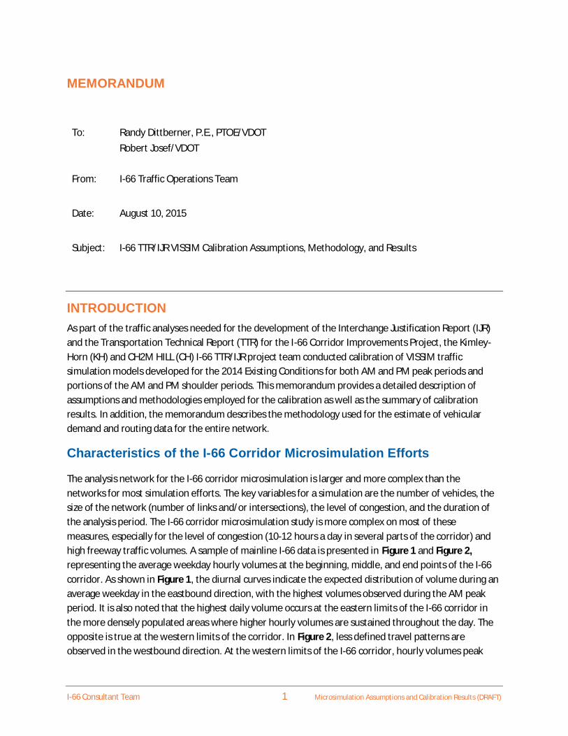
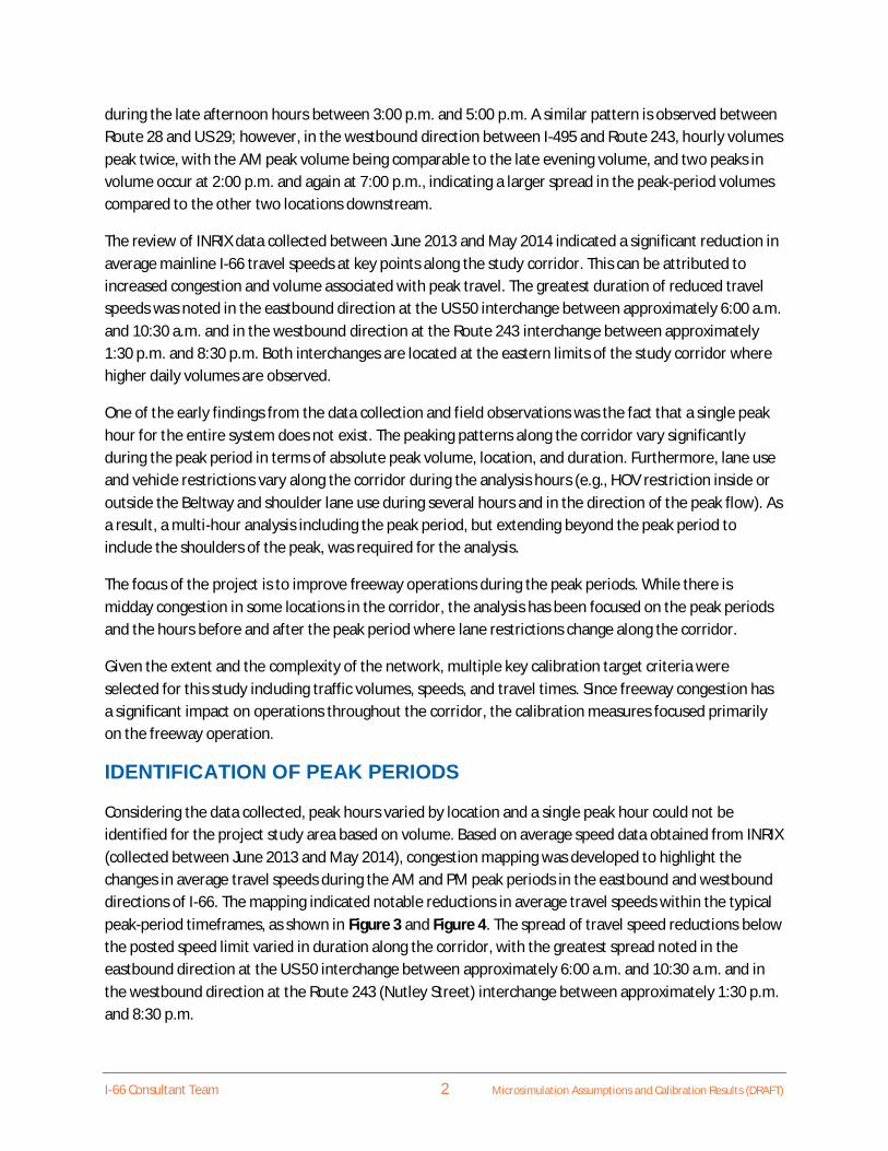
· As shown in Figure 8 and Figure 9, there is very little hourly variation among freeway mainlineand ramp volumes during the entire peak period. Furthermore, while volumes change slightly,the shape of the curve remains constant indicating that the proportions of traffic going from onespecific origin to multiple destinations would remain constant.
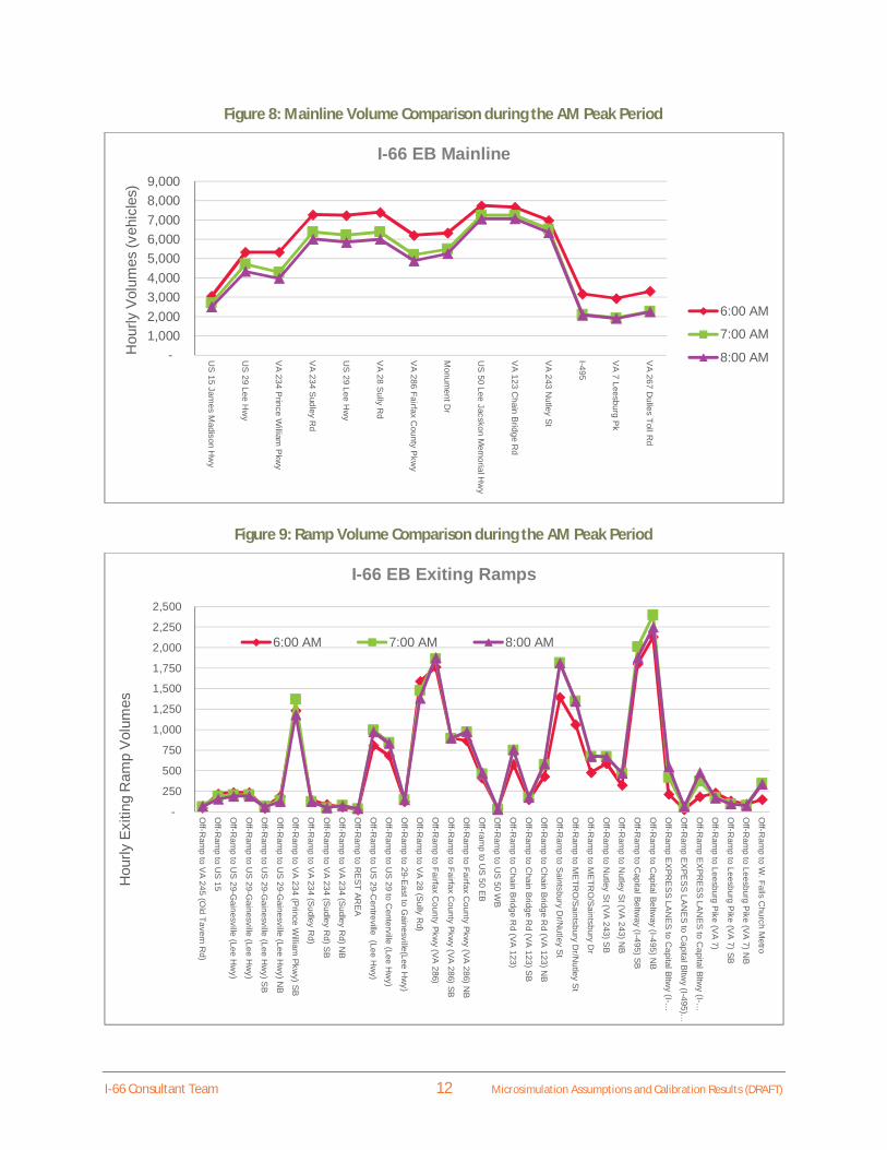
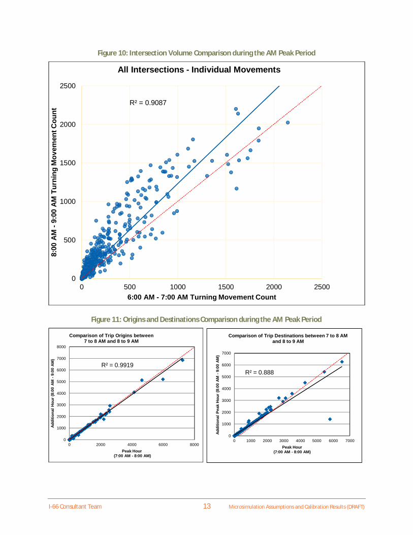
· Intersection volumes also remain roughly steady during the peak periods. Figure 10 shows thecomparison of intersection volumes between 6:00 to 7:00 a.m. and 8:00 to 9:00 a.m. An R-square of approximately 0.88 confirms this statement.
· Using VISUM, two different O-D tables were generated for two different sets of target volumesrelated to two different hours within the peak periods. The comparison of origins to origins anddestinations to destinations show very little variation. While comparing origins and destinations

I-66 Consultant Team 11 Microsimulation Assumptions and Calibration Results (DRAFT)
from two different O-D matrices is not necessarily a good indication of how similar thecorresponding assignments (associated paths) relate, the characteristics of the I-66 subareanetwork, where in general there is only one feasible path for each O-D pair, allows for theconclusion that if origins and destinations are similar between two different hours, theassignments will be similar as well. Figure 11 exemplifies the comparison of origins anddestinations for the AM peak period.
Based on these findings, a single routing scheme was used for the entire AM and PM peak periods. Inaddition, changes in volumes during the entire simulation period are captured in the model by enteringhalf-hour volume input distributions to all entry points in the network. In other words, while thefractions of volume going from any origin to other destinations remain the same during the peak period(e.g., single routing scheme), specific turning movement and link volumes change every half hour basedon input volume distributions.
I-66 Consultant Team 12 Microsimulation Assumptions and Calibration Results (DRAFT)
Figure 8: Mainline Volume Comparison during the AM Peak Period
Figure 9: Ramp Volume Comparison during the AM Peak Period
- 1,000 2,000 3,000 4,000 5,000 6,000 7,000 8,000 9,000
US
15Jam
esM
adisonH
wy
US
29Lee
Hw
y
VA
234P
rinceW
illiamP
kwy
VA
234S
udleyR
d
US
29Lee
Hw
y
VA
28S
ullyR
d
VA
286Fairfax
County
Pkw
y
Monum
entDr
US
50Lee
JacskonM
emorialH
wy
VA
123C
hainB
ridgeR
d
VA
243N
utleySt
I-495
VA
7Leesburg
Pk
VA
267D
ullesTollR
d
Hou
rlyV
olum
es(v
ehic
les)
I-66 EB Mainline
6:00 AM
7:00 AM
8:00 AM
-
250
500
750
1,000
1,250
1,500
1,750
2,000
2,250
2,500
Off-R
amp
toV
A245
(Old
TavernR
d)
Off-R
amp
toU
S15
Off-R
amp
toU
S29-G
ainesville(Lee
Hw
y)
Off-R
amp
toU
S29-G
ainesville(Lee
Hw
y)
Off-R
amp
toU
S29-G
ainesville(Lee
Hw
y)SB
Off-R
amp
toU
S29-G
ainesville(Lee
Hw
y)NB
Off-R
amp
toV
A234
(Prince
William
Pkwy)SB
Off-R
amp
toV
A234
(Sudley
Rd)
Off-R
amp
toV
A234
(Sudley
Rd)S
B
Off-R
amp
toV
A234
(Sudley
Rd)N
B
Off-R
amp
toR
EST
ARE
A
Off-R
amp
toU
S29-C
entreville(Lee
Hw
y)
Off-R
amp
toU
S29
toC
enterville(Lee
Hw
y)
Off-R
amp
to29-E
asttoG
ainesville(LeeH
wy)
Off-R
amp
toV
A28
(Sully
Rd)
Off-R
amp
toFairfax
County
Pkwy
(VA286)
Off-R
amp
toFairfax
County
Pkwy
(VA286)SB
Off-R
amp
toFairfax
County
Pkwy
(VA286)N
B
Off-ram
pto
US
50EB
Off-R
amp
toU
S50
WB
Off-R
amp
toC
hainB
ridgeR
d(VA
123)
Off-R
amp
toC
hainB
ridgeR
d(VA
123)SB
Off-R
amp
toC
hainB
ridgeR
d(VA
123)NB
Off-R
amp
toS
aintsburyD
r/Nutley
St
Off-R
amp
toM
ETR
O/S
aintsburyD
r/Nutley
St
Off-R
amp
toM
ETR
O/S
aintsburyD
r
Off-R
amp
toN
utleyS
t(VA243)S
B
Off-R
amp
toN
utleyS
t(VA243)N
B
Off-R
amp
toC
apitalBeltway
(I-495)SB
Off-R
amp
toC
apitalBeltway
(I-495)NB
Off-R
amp
EX
PRE
SS
LAN
ES
toC
apitalBltwy
(I-…
Off-R
amp
EX
PES
SLA
NE
Sto
CapitalBltw
y(I-495)…
Off-R
amp
EX
PRE
SS
LAN
ES
toC
apitalBltwy
(I-…
Off-R
amp
toLeesburg
Pike
(VA
7)
Off-R
amp
toLeesburg
Pike
(VA
7)SB
Off-R
amp
toLeesburg
Pike
(VA
7)NB
Off-R
amp
toW
.FallsC
hurchM
etroH
ourly
Exi
ting
Ram
pV
olum
es
I-66 EB Exiting Ramps
6:00 AM 7:00 AM 8:00 AM
I-66 Consultant Team 13 Microsimulation Assumptions and Calibration Results (DRAFT)
R² = 0.888
0
1000
2000
3000
4000
5000
6000
7000
0 1000 2000 3000 4000 5000 6000 7000
Addi
tiona
lPea
kH
our
(8:0
0AM
-9:0
0AM
)
Peak Hour(7:00 AM - 8:00 AM)
Comparison of Trip Destinations between 7 to 8 AMand 8 to 9 AM
Figure 10: Intersection Volume Comparison during the AM Peak Period
Figure 11: Origins and Destinations Comparison during the AM Peak Period
R² = 0.9087
0
500
1000
1500
2000
2500
0 500 1000 1500 2000 2500
8:00
AM
-9:0
0A
MTu
rnin
gM
ovem
entC
ount
6:00 AM - 7:00 AM Turning Movement Count
All Intersections - Individual Movements
R² = 0.9919
0
1000
2000
3000
4000
5000
6000
7000
8000
0 2000 4000 6000 8000
Addi
tiona
lHou
r(8:
00AM
-9:0
0AM
)
Peak Hour(7:00 AM - 8:00 AM)
Comparison of Trip Origins between7 to 8 AM and 8 to 9 AM

I-66 Consultant Team 14 Microsimulation Assumptions and Calibration Results (DRAFT)
As described above, the VISUM matrix estimation tool – TFLOWFUZZY – was used to accomplish the taskof synthetizing O-D data and producing the routing schemes for VISSIM. TFLOWFUZZY is a matrixestimation method used to adjust a given O-D matrix in such a way that the result of the assignmentclosely matches observed volumes at points within the network. In other words, TFLOWFUZZY resultswere calibrated to develop O-D tables that matched existing conditions.
TFLOWFUZZY characteristics are as follows:
· Link volumes, origin/destination travel demand and turning volumes can be combined forcorrection purposes.
· Counted data need not to be available for all links, zones and/or turning movements.· The statistical uncertainty of the count figures can be modeled explicitly by interpreting the
figures as Fuzzy Sets of input data.
One of the primary challenges with solving the matrix-correction problem is overcoming the fact thattraffic counts are inherently variable from one day to the next. If this variability is not taken intoaccount, the traffic counts obtain an inappropriate weight since any count only provides a snapshotsituation which is subject to considerable sampling error. For this reason, TFLOWFUZZY employs anapproach that models the counts as imprecise values based on Fuzzy Sets theory. If one knows, forexample, that the volume on a freeway section fluctuates by up to 10 percent on a day-to-day basis, thisvariability can be represented as bandwidths (i.e., tolerances). TFLOWFUZZY then replaces the exactcount values by Fuzzy Sets with varying bandwidths to solve the matrix-correction problem.
TFLOWFUZZY is applied within the context of an O-D assignment within VISUM. Consequently, VISUMassigns the demand between O-D pairs over a path or paths between the origin and destination. VISUMstores these paths, which can then be exported directly to VISSIM.
TFLOWFUZZY was applied to the I-66 study area to develop O-D matrices and corresponding path setsfor the AM and PM peak periods and the hours before and after the peak periods. The results of thisprocess are described in the following section.
O-D Synthesis Results
The quality of the solution produced by TFLOWFUZZY is best illustrated through a goodness-of-fit plot. Inthis project, these plots compare freeway, ramp and arterial link volumes (inputs) to modeled volumes(volumes produced by TFLOWFUZZY). The results are provided separately for the freeway and arterialstreets for the AM and PM peak periods in Figure 12 through Figure 15.
The R-square statistic measures how well TFLOWFUZZY was able to match the input volumes. In otherwords, R-square is the square of the correlation between the input volumes and modeled volumes. R-square can range between 0 and 1. A value closer to 1 indicates a better fit. For example, an R-squarevalue of 0.827 means that the fit explains 82.7 percent of the total variation in the data.

I-66 Consultant Team 15 Microsimulation Assumptions and Calibration Results (DRAFT)
TFLOWFUZZY approximated the input link volumes extremely well. The R-square value for the freewayand the arterial streets was 1.0 for both the AM peak period and for the PM peak period. Table 1summarizes the R-square results for all the analysis periods.
Another item of interest was the change between the original MWCOG seed O-D matrix and the matrixestimated by TFLOWFUZZY. During the AM peak hour, the TFLOWFUZZY O-D matrix resulted inapproximately 1410 less trips than the seed matrix. This reduction represented roughly 1 percent of thetotal trips (~118235) in the AM peak period seed O-D matrix. For the PM peak period, the TFLOWFUZZYproduced 22127 more trips than the seed O-D matrix. This increase represented roughly 19 percent ofthe total trips (~115155 trips) in the PM peak period seed O-D matrix.
When judging whether the previous results are acceptable, a number of items need to be considered.One of the primary inputs to this process was the subarea seed O-D matrix, which was derived from anO-D matrix developed to estimate regional travel patterns. This seed O-D matrix was then adjusted tofreeway, ramp, and arterial input volumes that more accurately reflect the conditions in the subareathan what can be reasonably expected from a model that is developed to reflect travel patterns on amuch larger regional scale. The R-square statistics indicated that the results of the TFLOWFUZZY processproduced an extremely good fit between the input and modeled volumes. It is also important tomention that the results from applying TFLOWFUZZY (O-D matrices and path sets) were a starting pointin VISSIM. When needed, additional calibration took place in VISSIM. Given the above considerations,the resulting TFLOWFUZZY O-D matrices and path sets were considered acceptable and transferred intoVISSIM.
Table 1: Summary of R-square Results from VISUM-TFLowFuzzy Process
Period R2 RMSNE1Average
Error(vehicles)
Comparisonwith Seed
MatrixAM Pre-peak 1.0 0.03 410 N/AAM Peak Period 1.0 0.03 242 1%AM Post-peak 1.0 0.03 421 N/APM Pre-peak 1.0 0.02 316 N/APM Peak Period 1.0 0.03 488 19%PM Post-peak 1.0 0.03 457 N/A
1 RMSNE: Root Mean Square Normalized Error2 R2: R Square (coefficient of determination)
The calibrated O-D matrix from VISUM was also disaggregated into four vehicle classes: auto, truck,HOV, and HOT. The disaggregation was based on the original seed matrices from the MWCOG model. Sixseed matrices were provided for each peak period: SOV, HOV2, HOV3+, HOT, LT, and HT.
Summing these individual O-D matrices produces a total O-D matrix. Dividing the SOV O-D matrix intothe total O-D matrix then results in the percentage of SOV trips between each O-D pair. Thesepercentages were applied to the calibrated VISUM O-D matrix to estimate an SOV matrix for VISSIM. Thesame approach was applied to HOVs and trucks. HOV2 and HOV3+, however, were combined into oneHOV class. The three truck classes were also combined into one class.

I-66 Consultant Team 16 Microsimulation Assumptions and Calibration Results (DRAFT)
Figure 12: Goodness of Fit for VISUM Results – AM Peak Period Regression Plot
Figure 13: Goodness of Fit for VISUM Results – AM Peak Period Absolute Error Plot
Target Volumes and Turning Movements
VISU
MVo
lum
esaf
terT
flow
fuzz
y
Target Volumes and Turning Movements
VISU
MVo
lum
esaf
terT
flow
fuzz
y

I-66 Consultant Team 17 Microsimulation Assumptions and Calibration Results (DRAFT)
Figure 14: Goodness of Fit for VISUM Results – PM Peak Period Regression Plot
Figure 15: Goodness of Fit for VISUM Results – PM Peak Period Absolute Error Plot
Target Volumes and Turning Movements
VISU
MVo
lum
esaf
terT
flow
fuzz
y
Target Volumes and Turning Movements
VISU
MVo
lum
esaf
terT
flow
fuzz
y

I-66 Consultant Team 18 Microsimulation Assumptions and Calibration Results (DRAFT)
VISSIM EXISTING CALIBRATIONThis section summarizes the effort conducted to calibrate existing AM and PM VISSIM models for the I-66 Corridor Improvements Project. The section includes a discussion of background for the calibrationplan, a summary of available calibration data, the calibration plan and criteria, and a summary of thecalibration results. The sections included are as follows:
· Purpose of a Calibration Plan· FHWA Guidelines and Calibration Criteria· Seeding Period· Number of Model Runs· General Approach for Calibration· Calibration Data Sources· Calibration Criteria· Calibration Parameters
Purpose of a Calibration Plan
The purpose of a simulation model is to investigate the effects of improvement alternatives.
Simulation models are an efficient tool for evaluating improvements but are most effective when thebase model matches real-world conditions. VISSIM, like all simulation models, was designed to beflexible enough that an analyst can calibrate the network to match the local conditions at a reasonablyaccurate level. It is well established that calibration is essential. FHWA has published “Guidelines forApplying Traffic Microsimulation Modeling Software” as part of its Traffic Analysis Toolbox (available athttp://ops.fhwa.dot.gov/trafficanalysistools/index.htm). The document “describes a process and acts asguidelines for the recommended use of traffic microsimulation software in transportation analyses.” Itincludes a seven-step process for microsimulation analysis. The fifth step is to compare model outputsto field data (and adjust model parameters) or calibration.
For complex projects, the specific steps and rules for calibration can vary greatly. A calibration plan isimportant to identify the structure for calibration and the framework for evaluating when calibration iscomplete. With a plan, the calibration approach can be agreed upon before starting work, and decision-makers can have confidence that calibration is complete.
For this project, the calibration plan will be the formal set of steps for calibration. The plan outlines thesteps that will be followed, the criteria used to evaluate calibration, and the related requirements (suchas the number of runs).
FHWA Guidelines and Calibration Criteria
The calibration guidance from the FHWA “Guidelines for Applying Traffic Microsimulation ModelingSoftware” document is described in this section.
I-66 Consultant Team 19 Microsimulation Assumptions and Calibration Results (DRAFT)
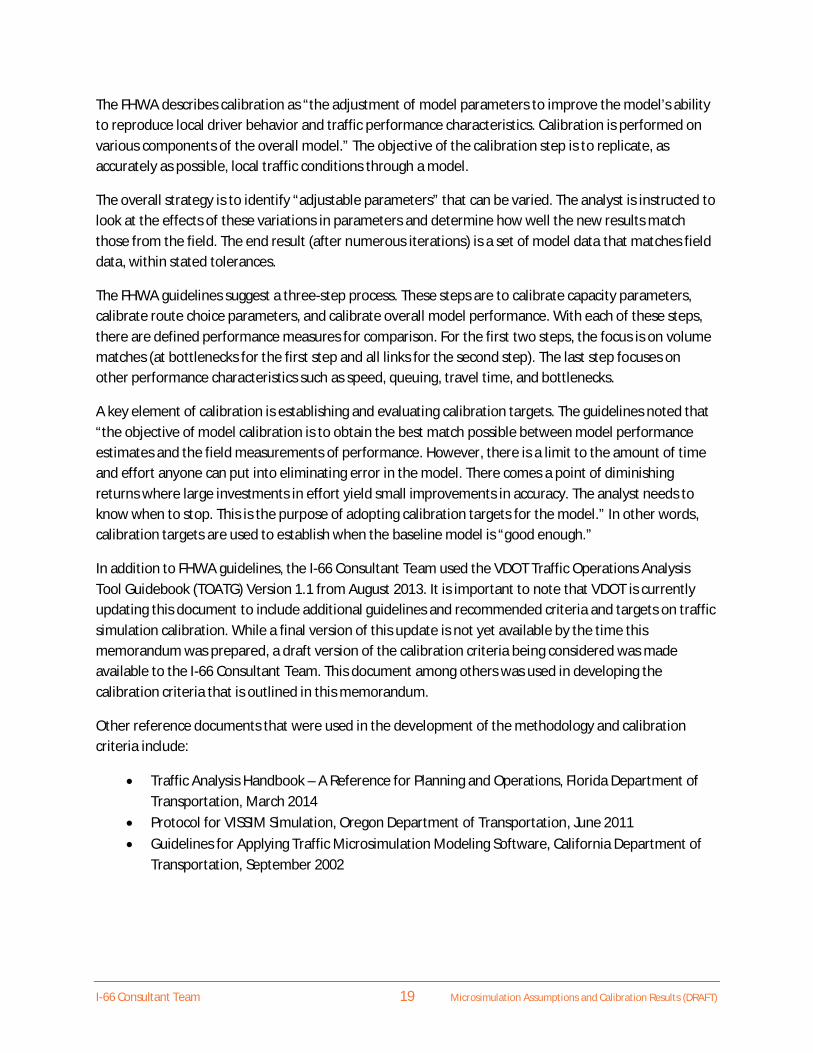
The FHWA describes calibration as “the adjustment of model parameters to improve the model’s abilityto reproduce local driver behavior and traffic performance characteristics. Calibration is performed onvarious components of the overall model.” The objective of the calibration step is to replicate, asaccurately as possible, local traffic conditions through a model.
The overall strategy is to identify “adjustable parameters” that can be varied. The analyst is instructed tolook at the effects of these variations in parameters and determine how well the new results matchthose from the field. The end result (after numerous iterations) is a set of model data that matches fielddata, within stated tolerances.
The FHWA guidelines suggest a three-step process. These steps are to calibrate capacity parameters,calibrate route choice parameters, and calibrate overall model performance. With each of these steps,there are defined performance measures for comparison. For the first two steps, the focus is on volumematches (at bottlenecks for the first step and all links for the second step). The last step focuses onother performance characteristics such as speed, queuing, travel time, and bottlenecks.
A key element of calibration is establishing and evaluating calibration targets. The guidelines noted that“the objective of model calibration is to obtain the best match possible between model performanceestimates and the field measurements of performance. However, there is a limit to the amount of timeand effort anyone can put into eliminating error in the model. There comes a point of diminishingreturns where large investments in effort yield small improvements in accuracy. The analyst needs toknow when to stop. This is the purpose of adopting calibration targets for the model.” In other words,calibration targets are used to establish when the baseline model is “good enough.”
In addition to FHWA guidelines, the I-66 Consultant Team used the VDOT Traffic Operations AnalysisTool Guidebook (TOATG) Version 1.1 from August 2013. It is important to note that VDOT is currentlyupdating this document to include additional guidelines and recommended criteria and targets on trafficsimulation calibration. While a final version of this update is not yet available by the time thismemorandum was prepared, a draft version of the calibration criteria being considered was madeavailable to the I-66 Consultant Team. This document among others was used in developing thecalibration criteria that is outlined in this memorandum.
Other reference documents that were used in the development of the methodology and calibrationcriteria include:
· Traffic Analysis Handbook – A Reference for Planning and Operations, Florida Department ofTransportation, March 2014
· Protocol for VISSIM Simulation, Oregon Department of Transportation, June 2011· Guidelines for Applying Traffic Microsimulation Modeling Software, California Department of
Transportation, September 2002

I-66 Consultant Team 20 Microsimulation Assumptions and Calibration Results (DRAFT)
Seeding PeriodThe seeding period is the period the model requires for the network-wide volumes to become stable.The length of the seeding period depends on numerous network factors like the size of the network andlevel of congestion. A seeding step is needed to ensure that output data is not collected until the end ofthe seeding period is reached. If it is collected earlier, simulation measures (e.g., travel time andcongestion) may be under-reported.
To determine the seeding period for the VISSIM simulation, two criteria were used:
· Time it takes a single vehicle to traverse the entire corridor during the peak hour· Volume loading analysis
For the first criteria, the time required for a vehicle to traverse the entire corridor was measured fromnine (9) simulations. Average times to traverse the corridor were 54 minutes in the AM peak androughly 1 hour the PM peak, both in the peak direction.
For the second criteria, nine (9) simulation runs were made, with the total volume in the networkreported every 2 and a half minutes. Then, the results for key locations in the network were plotted asshown in Figure 16. The figure indicates that the volumes in the network grow steady during the first2100 seconds (35 minutes) of the simulation. The network volumes transition to stable conditions afterthis period with normal increases and decreases for the rest of the simulation.
As a result of the above analysis, a seeding period of one hour was found to be adequate for both theAM and the PM models.

I-66 Consultant Team 21 Microsimulation Assumptions and Calibration Results (DRAFT)
Figure 16: Volume Loading Patterns for Key Mainline Segments
Number of Model Runs
Appendix B of the FHWA guidelines provides a summary of the need for multiple runs with amicrosimulation model: “Multiple repetitions of the same model are required because microsimulationresults will vary depending on the random number seed used in each run. The random number seed isused to select a sequence of random numbers that are used to make numerous decisions throughoutthe simulation run. The outcomes of all of these decisions will affect the simulation results. The resultsof each run will usually be close to the average of all of the runs; however, each run will be differentfrom the other.”
The challenge is to determine the number of runs. The FHWA guidelines suggest that the samplestandard deviation is the preferred approach. With this approach, a few runs are made to determine thestandard deviation of parameters of interest. Then, once the standard deviations are determined, thenumber of runs can be determined using a desired confidence interval. The total number of runsnecessary for the analysis will be determined based on the following:
% = 2 ∗ ( ⁄ ), √Where:
% = (1 – alpha)% confidence interval for the true mean, where alpha equals the probability of thetrue mean not lying within the confidence interval.
0
1000
2000
3000
4000
5000
6000
7000
8000
9000
0 1000 2000 3000 4000 5000 6000 7000 8000
Volu
me
(veh
/hr)
Simulation Time (Seconds)
Volume Loading - Eastbound I-66
I66EB - b/w Rt28 & Rt286 I66EB b/w University Blvd & Rt234I-66EB - East of Rt 15 I66EB Just before the BeltwayI66EB - East of the Beltway
Seeding Period Stable Volumes

I-66 Consultant Team 22 Microsimulation Assumptions and Calibration Results (DRAFT)
( ⁄ ), = Student’s t-statistic for the probability of a two-sided error summing to alpha with N-1degrees of freedom, where N equals the number of repetitions.
s = standard deviation of the model results.
While this is a straightforward approach, it becomes complex when there are multiple parameters ofinterest (such as different volumes and travel time comparisons). Therefore, for the I-66 corridor study,the following approach was used:
· The standard deviation of several key values was obtained by making nine runs of the VISSIMmodel. The key values were as follows:
o Average end-to-end travel time (AM peak period) for eastbound I-66 (*)o Average end-to-end travel time (AM peak period) for westbound I-66 (*)o Peak-period volume on eastbound I-66 mainline between US 15 and US 29o Peak-period volume on eastbound I-66 mainline between Route 28 and Route 286o Peak-period volume on eastbound I-66 mainline between Route 243 and I-495o Peak-period volume at same locations but westbound direction
(*) Note: these travel times may slightly differ from the overall travel times shown in the calibration results because thesecalculations were done at an interim phase and before the final calibration of the models. However, the values used for thecalculation of the number of runs are still valid.
· Confidence Interval for the analysis was assumed as:
o Volumes: +/- 10% of the sample mean at each of the above locationso Travel Time: +/- one Field Standard Deviation for the entire segment
· Level of Confidence: 99%
Table 2 and Table 3 summarize the results based on travel time criteria and volume criteria respectively.Based on these results, the adopted number of runs was 10.

I-66 Consultant Team 23 Microsimulation Assumptions and Calibration Results (DRAFT)
General Approach for Calibration
Many calibration projects have used different criteria, measures, and acceptance targets for calibrationpurposes. VDOT is currently working to generate its own criteria to be included in the VDOT TrafficOperations Analysis Tool Guidebook (TOATG)1. While these criteria are still not available, draft versionsof the performance measures and tolerance targets currently being evaluated were available to the I-66Consultant Team and used in developing the criteria for the I-66 corridor study.
Given the magnitude and complexity of the I-66 corridor simulation model, multiple measures ofperformance needed to be applied to calibrate the model. In the peak direction, I-66 operates underover-saturation for most of the peak period and for long portions of the corridor. Oversaturatedconditions makes calibration extremely challenging since travel speeds and other measures can changerapidly with small changes in traffic demand. The length of the corridor (35.7 miles) is another significantcontributor to the complexity of the calibration task. While matching certain calibration measures in theaggregate for the entire corridor is not too difficult, matching every measure in every segment is nearly
1 VDOT has recently changed the name of the guidebook previously known as TOATG to Traffic Operations and Safety AnalysisManual (TOSAM)
Error Tolerance 1 times field SDConfidence Interval (CI) =997.1 Eastbound
126.7 Westboundt= 3.36 for 99% Level of Confidence
Peak Hr End of Peak PeriodAVG 9000 12600 AVGAVERAGE TT 2544.50 3246.69 2892.21 2134.06 2160.15 2140.28
ST DEV 125.66 214.19 405.75 1.22 56.93 11.14Field St.Dev. 997.11 126.70
Field Mean TT 3977.6 1983.3SD/CI 0.12603 0.21481 0.40692 0.00965 0.44934 0.08791
N 1 3 8 1 10 1
Minimum Required Number of Runs = 10
Eastbound Travel Time (Seconds) Westbound Travel Time (Seconds)
CI=+/- 10% of sample mean t= 3.360 (9 runs - 99% level of confidence)
9000 12600 AVG 9000 12600 AVG 9000 12600 AVG 9000 12600 AVGEB 2141.6 2256.1 2198.8 151.9 77.0 76.6 428.3 451.2 439.8 6 2 2WB 1269.7 1202.9 1236.3 40.2 22.8 17.5 253.9 240.6 247.3 2 1 1EB 6183.0 5986.1 6084.6 93.5 90.0 35.3 1236.6 1197.2 1216.9 1 1 1WB 4409.7 4514.1 4461.9 57.2 226.9 123.1 881.9 902.8 892.4 1 3 1EB 5662.3 4559.7 5111.0 168.9 383.9 186.4 1132.5 911.9 1022.2 2 9 2WB 4949.5 5327.9 5138.7 68.6 59.9 53.5 989.9 1065.6 1027.7 1 1 1
Minimum Required Number of Runs = 9
Rt 15 to Rt 29 (Gainesville)
Rt 28 to Rt 286
Rt 243 to I-495
All Seeds Averages All Seeds St. Dev. All Seeds - NAll Seeds CISection Direction
Table 2: Number of Simulation Runs Required Based on Travel Time Criteria
Table 3: Number of Simulation Runs Required Based on Volume at Key Locations
I-66 Consultant Team 24 Microsimulation Assumptions and Calibration Results (DRAFT)
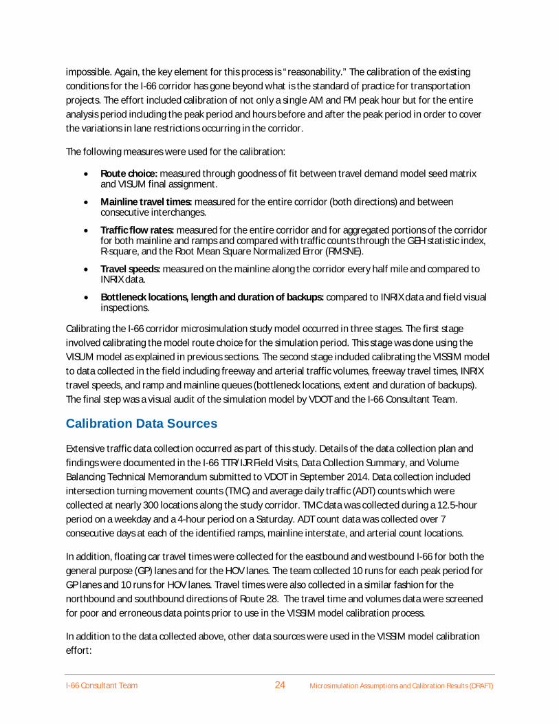
impossible. Again, the key element for this process is “reasonability.” The calibration of the existingconditions for the I-66 corridor has gone beyond what is the standard of practice for transportationprojects. The effort included calibration of not only a single AM and PM peak hour but for the entireanalysis period including the peak period and hours before and after the peak period in order to coverthe variations in lane restrictions occurring in the corridor.
The following measures were used for the calibration:
· Route choice: measured through goodness of fit between travel demand model seed matrixand VISUM final assignment.
· Mainline travel times: measured for the entire corridor (both directions) and betweenconsecutive interchanges.
· Traffic flow rates: measured for the entire corridor and for aggregated portions of the corridorfor both mainline and ramps and compared with traffic counts through the GEH statistic index,R-square, and the Root Mean Square Normalized Error (RMSNE).
· Travel speeds: measured on the mainline along the corridor every half mile and compared toINRIX data.
· Bottleneck locations, length and duration of backups: compared to INRIX data and field visualinspections.
Calibrating the I-66 corridor microsimulation study model occurred in three stages. The first stageinvolved calibrating the model route choice for the simulation period. This stage was done using theVISUM model as explained in previous sections. The second stage included calibrating the VISSIM modelto data collected in the field including freeway and arterial traffic volumes, freeway travel times, INRIXtravel speeds, and ramp and mainline queues (bottleneck locations, extent and duration of backups).The final step was a visual audit of the simulation model by VDOT and the I-66 Consultant Team.
Calibration Data Sources
Extensive traffic data collection occurred as part of this study. Details of the data collection plan andfindings were documented in the I-66 TTR/IJR Field Visits, Data Collection Summary, and VolumeBalancing Technical Memorandum submitted to VDOT in September 2014. Data collection includedintersection turning movement counts (TMC) and average daily traffic (ADT) counts which werecollected at nearly 300 locations along the study corridor. TMC data was collected during a 12.5-hourperiod on a weekday and a 4-hour period on a Saturday. ADT count data was collected over 7consecutive days at each of the identified ramps, mainline interstate, and arterial count locations.
In addition, floating car travel times were collected for the eastbound and westbound I-66 for both thegeneral purpose (GP) lanes and for the HOV lanes. The team collected 10 runs for each peak period forGP lanes and 10 runs for HOV lanes. Travel times were also collected in a similar fashion for thenorthbound and southbound directions of Route 28. The travel time and volumes data were screenedfor poor and erroneous data points prior to use in the VISSIM model calibration process.
In addition to the data collected above, other data sources were used in the VISSIM model calibrationeffort:

I-66 Consultant Team 25 Microsimulation Assumptions and Calibration Results (DRAFT)
· Existing signal timings were provided by VDOT. Questionable timings were field verified andchecked.
· Channelization was based on high-resolution aerial images, Google Earth Street view, and fieldverification. Videos were collected for all major freeway segments within the study area.
· Corridor congestion diagrams and speeds were compiled for the same days as the traffic countsdata collection. Average vehicle speeds were obtained from the University of Maryland Centerfor Advanced Transportation Technology (CATT). Their website serves as a warehouse for datacollected from INRIX which uses GPS probe vehicle data to determine average corridor speedsand travel times.
· Several field observations were conducted during peak periods by the Study Team on whichvideos and photos were taken to characterize typical operational conditions.
Route Choice Calibration Criteria
As described in the previous sections, origin-destination trip tables and associated paths weresynthesized using the VISUM model. The R-squared is a statistical measure of how close the data are tothe fitted regression line. In this case, the measure is used to compare link volumes generated by VISUMthrough the TFlowFuzzy methodology with target volumes from field counts. An R-squared of 0.98 orhigher was considered to indicate a reasonable calibration for route choice .
Travel Time Calibration Criteria
Travel time data were used to calibrate the existing conditions VISSIM model. Travel time data werecollected along I-66 for the entire corridor in both directions and for every segment betweeninterchanges. Travel time data were collected using the floating car method, where drivers traveled withthe prevailing traffic. On I-66, the breakpoints were the off-ramps, and times were recorded at the off-ramp gores. Travel times were also collected in a similar fashion for the northbound and southbounddirections of Route 28, from US 29 to Westfields Boulevard Interchange. Field travel times arecompared to simulation travel times based on the criteria summarized in Table 4.
Table 4: Calibration Criteria for Travel Time
Criterion Difference (SimulationVolume vs. Observed) Target
I-66 Mainline SegmentsWithin ± 1 minute Routes with observed travel times less
than 7 minutes
Within ± 15% Routes with observed travel timesgreater than 7 minutes

I-66 Consultant Team 26 Microsimulation Assumptions and Calibration Results (DRAFT)
Volume Calibration Criteria
Volumes from the model were compared to the traffic data collected in the field. Table 5 is a summaryof the volume calibration criteria for I-66 mainline, ramps, and intersections in this study.
Table 5: Summary of the Volume Calibration Criteria for I-66 Mainline, Ramps and Intersections
Travel Speed Calibration Criteria
Average link speeds from the model were compared to INRIX average speeds (INRIX data was obtainedand averaged for the same days when traffic data was collected on the field). Table 6 summarizes thecriteria for this measure.
Table 6: Calibration Criteria for Travel Speed
2 1The GEH Statistic is computed as follow:
= ( )( )/
Where: E= Model estimated Volume; V=Field Count
CriterionDifference
(Simulation Volumevs. Observed)
Target
Mainline segments, ramps, andintersections approach andcritical movements
Within 100 vph > 85% of cases for volumes < 400 vph
Within 15% > 85% of cases for volumes between 400vph to 2700 vph
Within ± 400 vph > 85% of cases for volumes > 2700 vph
Each mainline segments GEH2 < 5.0 85% of all mainline segments
Aggregate of all mainlinesegments RMSNE >0.15
CriterionDifference
(Simulation Speed vs. Observed)Target
I-66 Mainline SegmentsWithin ± 10 mph On at least the top 80% of
network links by volumes
RMSNE >0.20

I-66 Consultant Team 27 Microsimulation Assumptions and Calibration Results (DRAFT)
Calibration Criteria for Bottleneck Locations, Length and Duration ofBackups
The final calibration stage was the visual audit component of the simulation model, that is how well thesimulation model is operating visually and ensuring the model is replicating field observations.Bottlenecks and queuing are the key elements of the visual audits. While bottlenecks and queuing affectvolume and travel times, they also require a separate focus during calibration.
The first and most important characteristic of a bottleneck is its occurrence at a particular location.Bottlenecks may be formed due to factors such as ramp merges/diverges, lane drops, road construction,increases in traffic demand, or even crashes which cause a reduction in capacity. The bottlenecksformed due to temporary traffic conditions such as vehicle crashes are isolated incidents whereas theones formed due to roadway geometric/design changes and increases in demand occur regularly. Theserecurring bottlenecks do not necessarily occur every day, and they may start and stop based on dailytraffic variations.
The second defining characteristic of a bottleneck is the length of the queuing. It is defined as thelength/extent of the queue starting from the beginning of the bottleneck extending back to wheremotorists start to slow from their desired free-flow speed.
The third defining characteristic of a bottleneck is duration and start time of a bottleneck, which are thetemporal components of the bottleneck at particular locations. In the effort to understand what causesa bottleneck and find potential solutions, it is important to know where the bottleneck actuallyterminates and free-flow conditions are restored. This is typically found where speeds increase fromcongested speeds to 30 to 50 miles per hour, often occurring over a very short distance.
Bottlenecks can be assessed by analyzing the speed profile data obtained from various sources includingimbedded freeway induction loops, GPS systems, and other data archival systems. The VISSIMcalibration utilized speed and congestion information from INRIX, a leading provider of trafficinformation. Freeway speed information was collected from INRIX data to determine bottlenecklocations, duration, and length of queues in the study area. This information was aggregated into speeddiagrams or “brain scans.” These brain scans are based on the same days where traffic counts and traveltime runs were conducted in the field.
Calibration Parameters
Calibrating the AM and PM peak period I-66 corridor VISSIM models involved adjusting specificparameters to achieve the target volume, speeds, and travel time thresholds. The primary parametersthat were adjusted included the following.

I-66 Consultant Team 28 Microsimulation Assumptions and Calibration Results (DRAFT)
Speed Distributions: Typically, the VISSIM model was coded with a desired speed distribution set tomatch posted speed limits. Speed distributions were established that 85 percent of vehicles would travelat or above the posted speed limit, and the maximum speed for each distribution was capped to 10 mphabove the posted speed limit. To better match field observed speeds, speed distributions were adjustedas needed during each hour within the simulation period to more closely reflect the speeds reportedfrom the floating car studies. In most cases, free-flow speeds were increased upward from the originalspeed distributions indicating that, under unconstrained conditions, most drivers travel faster than theposted speed limit. In addition, as several locations in the corridor operate at constrained conditionsduring the AM and PM peak periods, free-flow speeds at the roadway network termini were reduced toreplicate the conditions observed and measured in the field. Free-flow speed reductions aid inreplicating the stop-and-go traffic conditions that occur regularly beyond the edges of the roadwaynetwork used in the VISSIM microsimulation models. Modification of free-flow speeds at the edge of thenetwork to help replicate downstream and upstream congestion is an industry-acceptable techniqueused in calibration of microsimulation models.
Lane Change Distances: Lane-change look-back distances is the distance in the VISSIM model where avehicle will start attempting to make a lane change to a target lane prior to an off-ramp, a lane drop, orchange in direction in travel. This lane-change distance is a parameter on every connector in the VISSIMnetwork, and its default change distance value is 656 feet. This distance is typically acceptable for lowspeed, intersection turning movements; however, it would provide extremely challenging lane changingbehavior for freeway diverges and lane drops. As a starting point in the VISSIM model, the lane-changedistance for diverges and lane drops was modified to match the first field observed way-finding sign.This distance is typically one mile upstream of an off-ramp. The parameter was then adjusted on a case-by-case basis at different locations with the goal of calibrating existing queues, speeds, and travel timeswithin the study area.
Driver Behavior – Car-Following Adjustments: VISSIM incorporates two different car-following models –one for freeways and one for arterials. In combination with other operational parameters, analysts havethe ability to adjust these parameters as needed to achieve desired flow conditions. In addition to otherparameters, such as vehicle speed, heavy vehicle percentage, and number of lanes, the car-followingparameters effectively change roadway capacity, vehicle spacing and headways.
The car-following parameters adjusted during the calibration process for freeways were modified basedon previous experiences with similar type of networks and operations, engineering judgment, and fieldobservations. They were typically adjusted if a field condition (i.e. poor vertical sight distance, narrowlateral clearances, etc.) warranted a change from VISSIM default parameters. From the list of car-following parameters that can be modified, three are the most sensitive for calibration:
· CC0 – Standstill Distance is defined as the desired distance between stopped cars. Thisparameter is typically used to increase or decrease vehicle spacing while vehicles are in queueand is used during calibration to affect queue duration and length.
· CC1 – Headway Time is not a direct measure of headway time but rather a factor that affects thefollowing (minimum desired safety) distance. The higher this value, the more cautious the driveris; thus reducing capacity. In the case of high volumes, it is the following distance that has the
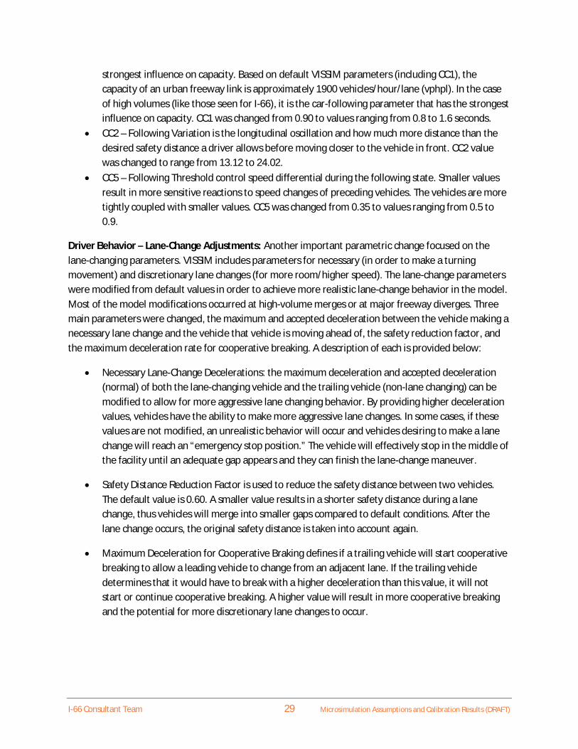
I-66 Consultant Team 29 Microsimulation Assumptions and Calibration Results (DRAFT)
strongest influence on capacity. Based on default VISSIM parameters (including CC1), thecapacity of an urban freeway link is approximately 1900 vehicles/hour/lane (vphpl). In the caseof high volumes (like those seen for I-66), it is the car-following parameter that has the strongestinfluence on capacity. CC1 was changed from 0.90 to values ranging from 0.8 to 1.6 seconds.
· CC2 – Following Variation is the longitudinal oscillation and how much more distance than thedesired safety distance a driver allows before moving closer to the vehicle in front. CC2 valuewas changed to range from 13.12 to 24.02.
· CC5 – Following Threshold control speed differential during the following state. Smaller valuesresult in more sensitive reactions to speed changes of preceding vehicles. The vehicles are moretightly coupled with smaller values. CC5 was changed from 0.35 to values ranging from 0.5 to0.9.
Driver Behavior – Lane-Change Adjustments: Another important parametric change focused on thelane-changing parameters. VISSIM includes parameters for necessary (in order to make a turningmovement) and discretionary lane changes (for more room/higher speed). The lane-change parameterswere modified from default values in order to achieve more realistic lane-change behavior in the model.Most of the model modifications occurred at high-volume merges or at major freeway diverges. Threemain parameters were changed, the maximum and accepted deceleration between the vehicle making anecessary lane change and the vehicle that vehicle is moving ahead of, the safety reduction factor, andthe maximum deceleration rate for cooperative breaking. A description of each is provided below:
· Necessary Lane-Change Decelerations: the maximum deceleration and accepted deceleration(normal) of both the lane-changing vehicle and the trailing vehicle (non-lane changing) can bemodified to allow for more aggressive lane changing behavior. By providing higher decelerationvalues, vehicles have the ability to make more aggressive lane changes. In some cases, if thesevalues are not modified, an unrealistic behavior will occur and vehicles desiring to make a lanechange will reach an “emergency stop position.” The vehicle will effectively stop in the middle ofthe facility until an adequate gap appears and they can finish the lane-change maneuver.
· Safety Distance Reduction Factor is used to reduce the safety distance between two vehicles.The default value is 0.60. A smaller value results in a shorter safety distance during a lanechange, thus vehicles will merge into smaller gaps compared to default conditions. After thelane change occurs, the original safety distance is taken into account again.
· Maximum Deceleration for Cooperative Braking defines if a trailing vehicle will start cooperativebreaking to allow a leading vehicle to change from an adjacent lane. If the trailing vehicledetermines that it would have to break with a higher deceleration than this value, it will notstart or continue cooperative breaking. A higher value will result in more cooperative breakingand the potential for more discretionary lane changes to occur.

I-66 Consultant Team 30 Microsimulation Assumptions and Calibration Results (DRAFT)
In areas where significant lane-change conditions were identified, default driving behavior was adjustedin the model to account for more aggressive and/or cooperative lane-change-behavior drivers.Adjustments in the lane-change parameters were used to better replicate actual driver behavior undercongested and severe weaving conditions in the simulation model.
It is important to note that many of these changes are link specific to account for the variations ingeometric and accompanying driver behaviors along the corridor. Furthermore, values may differbetween the AM and PM peak hours since motorists will change their lane-change aggressiveness basedon prevailing traffic conditions.

I-66 Consultant Team 31 Microsimulation Assumptions and Calibration Results (DRAFT)
CALIBRATION RESULTS
AM Existing ModelI-66 TRAVEL TIME CALIBRATION RESULTS
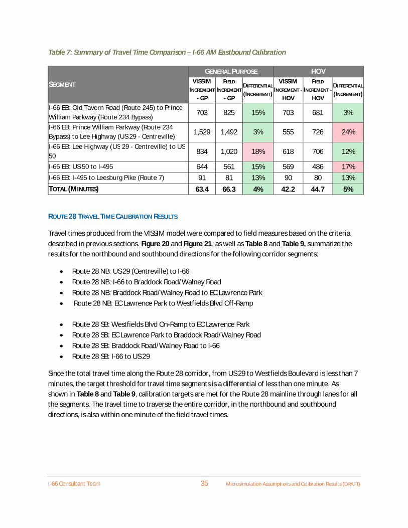
Travel times produced from the VISSIM model were compared to field measures based on the criteriadescribed in previous sections. Figure 17 and Table 7 summarize the results for the eastbound directionfor the following corridor segments:
· I-66 EB: Old Tavern Road (Route 245) to Prince William Parkway (Route 234 Bypass)· I-66 EB: Prince William Parkway (Route 234 Bypass) to Lee Highway (US 29 - Centreville)· I-66 EB: Lee Highway (US 29 - Centreville) to US 50· I-66 EB: US 50 to I-495· I-66 EB: I-495 to Leesburg Pike (Route 7)
In Figure 17, calibration targets are depicted with high-low bars on field travel-time measures. As shownin this figure and on Table 7, calibration targets are met for the general purpose lanes for all thesegments. The travel time of the general purpose lanes for the entire corridor is within 4 percent of thefield travel times. HOV lanes show higher differences between VISSIM and field values with twosegments resulting in differences greater than 15 percent. The HOV lane segment from Prince WilliamParkway (Route 234 Bypass) to Lee Highway (US 29) is 24 percent lower compared to the field traveltimes while the HOV lane segment from US 50 to I-495 is 17 percent higher compared to the field traveltimes. While the difference is higher than the target specified in the criteria, it is important to note whenthe entire corridor is compared, the differences in travel time between VISSIM and field measures forthe HOV lane is only 5 percent. In the westbound direction four of five segments met the calibrationtargets. The segment from US 50 to US 29 (Centreville) is 17 percent higher compared to the field traveltimes.

I-66 Consultant Team 32 Microsimulation Assumptions and Calibration Results (DRAFT)
Figure 17: Travel Time Results – AM Combined Corridor Segments
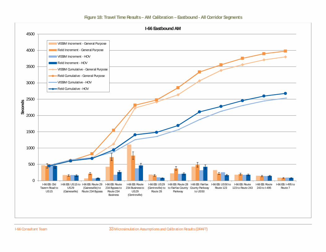
Figure 18 and Figure 19 summarize the results for the entire corridor for every segment betweeninterchanges for both eastbound and westbound respectively. The figures show that there is a very closematch between the VISSIM travel times and the field travel times throughout the corridor in bothdirections for general purpose and HOV lanes.
0
200
400
600
800
1000
1200
1400
1600
1800
2000
I-66 EB: Old TavernRoad to Route 234
Bypass
I-66 EB: Route 234Bypass to US 29
(Centreville)
I-66 EB:US 29(Centreville) to US
50
I-66 EB: US 50 to I-495
I-66 EB: I-495 toRoute 7
Seco
nds
I-66 Eastbound AM
VISSIM Increment - General Purpose
Field Increment - General Purpose
VISSIM Increment - HOV
Field Increment - HOV
I-66 Consultant Team 33 Microsimulation Assumptions and Calibration Results (DRAFT)
Figure 18: Travel Time Results – AM Calibration – Eastbound - All Corridor Segments
0
500
1000
1500
2000
2500
3000
3500
4000
4500
I-66 EB: OldTavern Road to
US 15
I-66 EB: US 15 toUS 29
(Gainesville)
I-66 EB: Route 29(Gainesville) to
Route 234 Bypass
I-66 EB: Route234 Bypass to
Route 234Business
I-66 EB: Route234 Business to
US 29(Centreville)
I-66 EB: US 29(Centreville) to
Route 28
I-66 EB: Route 28to Fairfax County
Parkway
I-66 EB: FairfaxCounty Parkway
to US 50
I-66 EB: US 50 toRoute 123
I-66 EB: Route123 to Route 243
I-66 EB: Route243 to I-495
I-66 EB: I-495 toRoute 7
Seco
nds
I-66 Eastbound AM
VISSIM Increment - General Purpose
Field Increment - General Purpose
VISSIM Increment - HOV
Field Increment - HOV
VISSIM Cumulative - General Purpose
Field Cumulative - General Purpose
VISSIM Cumulative - HOV
Field Cumulative - HOV

I-66 Consultant Team 34 Microsimulation Assumptions and Calibration Results (DRAFT)
Figure 19: Travel Time Results – AM Calibration – Westbound - All Corridor Segments
0
500
1000
1500
2000
2500
I-66: Dulles TollRoad to Route 7
I-66 WB: Route 7to I-495
I-66 WB: I-495 toRoute 243
I-66 WB: Route243 to Route 123
I-66 WB: Route123 to US 50
I-66 WB: US 50to Fairfax County
Parkway
I-66 WB: FairfaxCounty Parkway
to Sully Road(Route 28 )
I-66 WB: Route28 to US 29(Centreville)
I-66 WB: US 29(Centreville) to
Sudley Road(Route 234Business)
I-66 WB: SudleyRoad (Route
234) to Route234 Bypass
I-66 WB: Route234 Bypass to US29 (Gainesville)
I-66 WB: US 29(Gainesville) to
US 15
I-66 WB: US 15to Old Tavern
Road
Seco
nds
I-66 Westbound AM
VISSIM Increment
Field Increment
VISSIM Cumulative
Field Cumulative
I-66 Consultant Team 35 Microsimulation Assumptions and Calibration Results (DRAFT)
Table 7: Summary of Travel Time Comparison – I-66 AM Eastbound Calibration
ROUTE 28 TRAVEL TIME CALIBRATION RESULTS
Travel times produced from the VISSIM model were compared to field measures based on the criteriadescribed in previous sections. Figure 20 and Figure 21, as well as Table 8 and Table 9, summarize theresults for the northbound and southbound directions for the following corridor segments:
· Route 28 NB: US 29 (Centreville) to I-66· Route 28 NB: I-66 to Braddock Road/Walney Road· Route 28 NB: Braddock Road/Walney Road to EC Lawrence Park· Route 28 NB: EC Lawrence Park to Westfields Blvd Off-Ramp
· Route 28 SB: Westfields Blvd On-Ramp to EC Lawrence Park· Route 28 SB: EC Lawrence Park to Braddock Road/Walney Road· Route 28 SB: Braddock Road/Walney Road to I-66· Route 28 SB: I-66 to US 29
Since the total travel time along the Route 28 corridor, from US 29 to Westfields Boulevard is less than 7minutes, the target threshold for travel time segments is a differential of less than one minute. Asshown in Table 8 and Table 9, calibration targets are met for the Route 28 mainline through lanes for allthe segments. The travel time to traverse the entire corridor, in the northbound and southbounddirections, is also within one minute of the field travel times.
SEGMENT
GENERAL PURPOSE HOVVISSIM
INCREMENT
- GP
FIELD
INCREMENT
- GP
DIFFERENTIAL
(INCREMENT)
VISSIMINCREMENT -
HOV
FIELD
INCREMENT -HOV
DIFFERENTIAL
(INCREMENT)
I-66 EB: Old Tavern Road (Route 245) to PrinceWilliam Parkway (Route 234 Bypass)
703 825 15% 703 681 3%
I-66 EB: Prince William Parkway (Route 234Bypass) to Lee Highway (US 29 - Centreville)
1,529 1,492 3% 555 726 24%
I-66 EB: Lee Highway (US 29 - Centreville) to US50
834 1,020 18% 618 706 12%
I-66 EB: US 50 to I-495 644 561 15% 569 486 17%I-66 EB: I-495 to Leesburg Pike (Route 7) 91 81 13% 90 80 13%TOTAL (MINUTES) 63.4 66.3 4% 42.2 44.7 5%

I-66 Consultant Team 36 Microsimulation Assumptions and Calibration Results (DRAFT)
Figure 20: Route 28 Travel Time Results – AM Calibration – Northbound
Figure 21: Route 28 Travel Time Results – AM Calibration – Southbound
0
50
100
150
200
250
Route 28 NB: US 29 to I-66 Route 28 NB: I-66 to BraddockRoad/Walney Road
Route 28 NB: BraddockRoad/Walney Road to EC
Lawrence Park
Route 28 NB: EC Lawrence Parkto Westfields Blvd Off-Ramp
Seco
nds
Route 28 Northbound AM Travel Time Comparison
VISSIM IncrementField IncrementVISSIM CumulativeField Cumulative
0
20
40
60
80
100
120
140
160
180
Route 28 SB: Westfields Blvd On-Ramp to EC Lawrence Park
Route 28 SB: EC Lawrence Park toBraddock Road/Walney Road
Route 28 SB: BraddockRoad/Walney Road to I-66
Route 28 SB: I-66 to US 29
Seco
nds
Route 28 Southbound AM Travel Time ComparisonVISSIM IncrementField IncrementVISSIM CumulativeField Cumulative

I-66 Consultant Team 37 Microsimulation Assumptions and Calibration Results (DRAFT)
Table 8: Summary of Travel Time Comparison – Route 28 AM Northbound Calibration
SEGMENT
GENERAL PURPOSEVISSIM
INCREMENT
(SECONDS)
FIELD
INCREMENT
(SECONDS)
DIFFERENTIAL
(MINUTE)
Route 28 NB: US 29 to I-66 31 40 -0.15
Route 28 NB: I-66 to Braddock Road/Walney Road 65 91 -0.43
Route 28 NB: Braddock Road/Walney Road to EC Lawrence Park 47 59 -0.19
Route 28 NB: EC Lawrence Park to Westfields Blvd Off-Ramp 44 44 0.00
TOTAL (MINUTES) 3.12 3.90 -0.78
Table 9: Summary of Travel Time Comparison – Route 28 AM Southbound Calibration
SEGMENT
GENERAL PURPOSEVISSIM
INCREMENT
(SECONDS)
FIELD
INCREMENT
(SECONDS)
DIFFERENTIAL
(MINUTE)
Route 28 SB: Westfields Blvd On-Ramp to EC Lawrence Park 34 37 -0.05
Route 28 SB: EC Lawrence Park to Braddock Road/Walney Road 63 55 0.14
Route 28 SB: Braddock Road/Walney Road to I-66 43 35 0.13
Route 28 SB: I-66 to US 29 21 18 0.04
TOTAL (MINUTES) 2.69 2.42 0.27
VOLUME CALIBRATION RESULTS
Throughput volumes produced by the VISSIM model were compared to balanced traffic counts based onthe criteria described in previous sections. Table 10 summarizes the comparison based on the GEHcriteria for the entire I-66 corridor, for combined segments for both eastbound and westbounddirection, for I-495 segments both for northbound and southbound directions, and for Route 28segments both for northbound and southbound directions. The results are grouped by freeway mainlinesegments and ramps. Table 10 also includes comparison results based on GEH criteria for all arterialapproaches within the study area. In the eastbound direction, there are segments which do not meetthe GEH targets; however, for the overall, 84 percent of the segments meet the GEH criteria. The targetfor GEH was to meet the criteria for 85 percent of the mainline segments and ramps. The model is veryclose to the target. Also as seen in Figure 22 below, more than 88 percent of the eastbound links meetthe volume difference thresholds. Also based on Table 10, the mainline segments, ramps in the I-66westbound direction, the I-495 northbound and southbound direction, the Route 28 southbounddirection, and the intersection approaches all meet the target of 85 percent or more segments meetingthe GEH criteria.

I-66 Consultant Team 38 Microsimulation Assumptions and Calibration Results (DRAFT)
Table 10: Summary of Volume Comparison – I-66/I-495/Route 28 AM Calibration
Section ID SegmentNumber of Locations Locations Meeting GEH Percent Meeting GEH
Mainline Ramps Overall Mainline Ramps Overall Mainline Ramps OverallOverall Study Area 186 237 423 164 212 376 90% 89% 89%
EB
1I-66: Old Tavern Road (Route 245) toPrince William Parkway (Route 234Bypass)
14 17 31 14 16 30 100% 94% 97%
2I-66: Prince William Parkway (Route 234Bypass) to Lee Highway (US 29 -Centreville)
15 14 29 13 11 24 87% 79% 83%
3 I-66: Lee Highway (US 29 - Centreville) toUS 50 15 23 38 12 23 35 80% 100% 92%
4 I-66: US 50 to I-495 15 30 45 12 28 40 80% 93% 89%5 I-66: I-495 to Dulles Toll Road 7 9 16 1 9 10 14% 100% 63%
Total: I-66 Eastbound 66 93 159 52 87 139 79% 94% 87%
WB
6 I-66: Dulles Toll Road to I-495 13 12 25 13 12 25 100% 100% 100%7 I-66: I-495 to US 50 15 23 38 15 23 38 100% 100% 100%
8 I-66: US 50 to Lee Highway (US 29 -Centreville) 13 18 31 13 13 26 100% 72% 84%
9I-66: Lee Highway (US 29 - Centreville) toPrince William Parkway (Route 234Bypass)
14 7 21 14 7 21 100% 100% 100%
10 I-66: Prince William Parkway (Route 234Bypass) to Old Tavern Road (Route 245) 15 11 26 15 11 26 100% 100% 100%
Total: I-66 Westbound 70 71 141 70 66 136 100% 93% 97%
NB 11 I-495 Entire Corridor 22 32 54 21 25 46 95% 78% 85%
SB 12 I-495 Entire Corridor 28 41 69 26 34 60 93% 83% 87%
NB 13 Route 28 Entire Corridor 10 10 20 6 7 13 60% 70% 65%
SB 14 Route 28 Entire Corridor 11 9 20 11 9 20 100% 100% 100%
Arterial Approaches 281 259 92%

I-66 Consultant Team 39 Microsimulation Assumptions and Calibration Results (DRAFT)
Figure 22 below depicts the percentage of links meeting the GEH criteria as well as the volumedifference criteria (see targets in Table 5). Close to 85 percent of the links meet the GEH criteria while 88percent or more links meet the volume differential target criteria.
Figure 22: Freeway Volume Results – AM Calibration - All Corridor Segments
Similar to the freeway volumes, intersection approach volumes were compared to traffic counts for bothGEH and volume difference criteria. Figure 23 illustrates the results for the AM peak hour. As shown, 90percent of approaches meet the GEH and the volume differential criteria.
Figure 23: Arterial Volume Results – AM Calibration – All Corridor Segments
139,87%
20, 13%
Locations with GEH <5 Locations with GEH > 5
146,92%
13,8%
Volume Difference Threshold Met
Volume Difference Threshold Not Met
259,92%
22,8%
Approaches with GEH <5
Approaches with GEH >5
262,93%
19,7%
Volume Differential: Threshold Met
Volume Differential: Threshold Not Met

I-66 Consultant Team 40 Microsimulation Assumptions and Calibration Results (DRAFT)
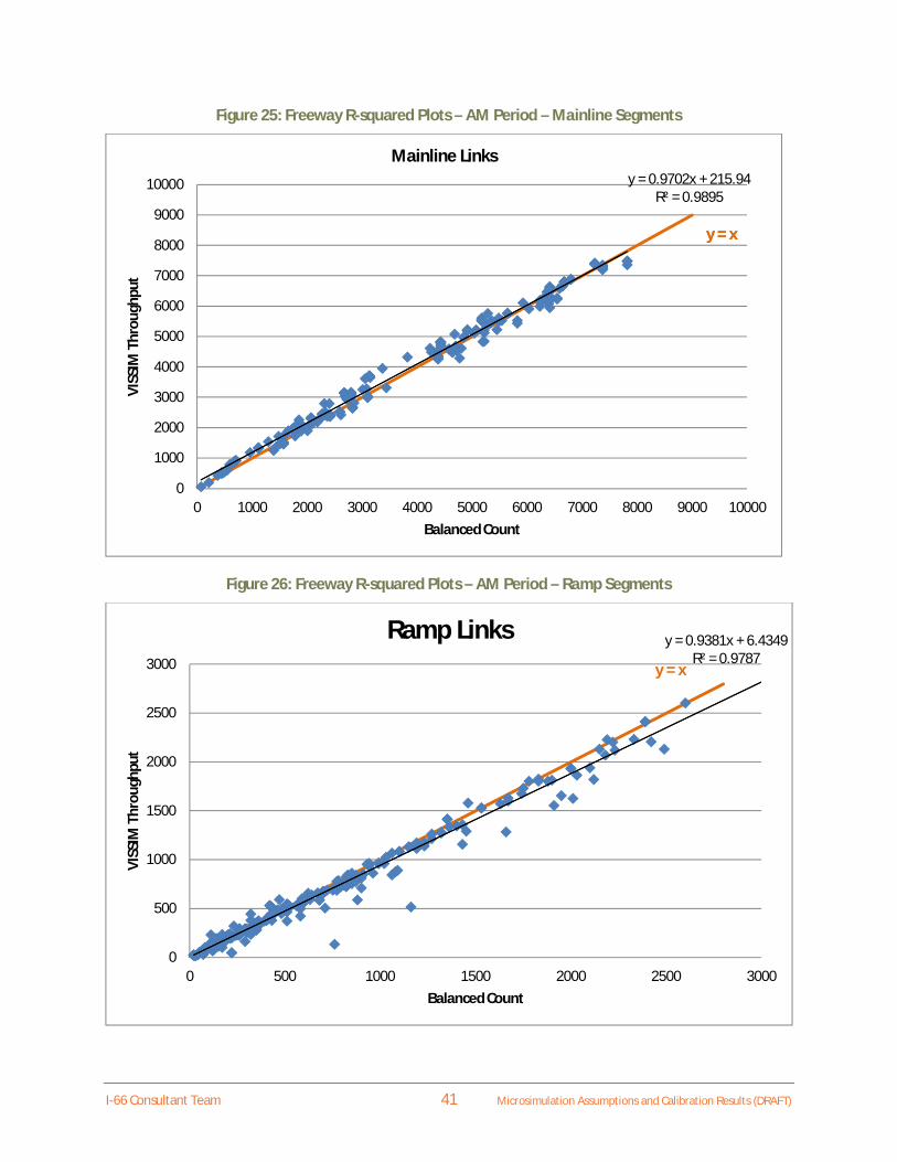
In addition, R-square plots were developed to test the correlation between VISSIM throughput and fieldcounts. Figure 24, Figure 25, and Figure 26 depict the results for the AM period for all freeway links,mainline segments, and ramp segments respectively. As shown in these figures, R-squared resultsranging between 0.98 and 0.99 confirm a good fit between model throughputs and field counts.
Figure 24: Freeway R-squared Plots – AM Period – All Corridor Segments
y = 1.0073x + 9.2353R² = 0.9931
0
1000
2000
3000
4000
5000
6000
7000
8000
9000
10000
0 1000 2000 3000 4000 5000 6000 7000 8000 9000 10000
VISS
IMTh
roug
hput
Balanced Count
All Freeway/Ramp Links
y = x
I-66 Consultant Team 41 Microsimulation Assumptions and Calibration Results (DRAFT)
Figure 25: Freeway R-squared Plots – AM Period – Mainline Segments
Figure 26: Freeway R-squared Plots – AM Period – Ramp Segments
y = 0.9702x + 215.94R² = 0.9895
0
1000
2000
3000
4000
5000
6000
7000
8000
9000
10000
0 1000 2000 3000 4000 5000 6000 7000 8000 9000 10000
VISS
IMTh
roug
hput
Balanced Count
Mainline Links
y = xy = x
y = 0.9381x + 6.4349R² = 0.9787
0
500
1000
1500
2000
2500
3000
0 500 1000 1500 2000 2500 3000
VISS
IMTh
roug
hput
Balanced Count
Ramp Linksy = x

I-66 Consultant Team 42 Microsimulation Assumptions and Calibration Results (DRAFT)
SPEED CALIBRATION
Average speeds were compared to INRIX speeds collected for similar days when traffic data wascollected on the field. Table 11 summarizes the results of this comparison. Based on the criteriadescribed in Table 6, while several segments closely match INRIX speeds, others fall short. In theeastbound direction, almost 80 percent of the links meet the criteria with some segments betweenPrince William Parkway (Route 234 Bypass) and US 50 not meeting the speed criteria. However, in thewestbound I-66 direction and along northbound and southbound I-495, more than 85 percent of thelinks match the criteria. INRIX data was not gathered for Route 28, and therefore, that corridor was notincorporated into the speed calibration. Variations on individual segments are expected for severalreasons, the most important being the fact that INRIX data is less reliable than travel time field data thusit was used as a second or third tier in the calibration priority measures. INRIX data is an average speedof all lanes including auxiliary and declaration/acceleration lane speeds. In locations where there is aspill back of a ramp which mainly affects the exiting lanes, INRIX speeds will be lower while the traveltime speeds would be greater if they were conducted in lanes that were not affected by the spill back.
BOTTLENECK LOCATIONS, LENGTH AND DURATION OF BACKUPS
Comparison of INRIX data with travel speeds measured in the model every half mile provided a veryuseful way for checking bottleneck locations as well as the extent and temporal distribution of mainlinequeues and overall congestion. Figure 27 depicts the “heat” diagrams for the entire corridor for theeastbound direction in the AM period. As shown, there is a very reasonable match between INRIX andVISSIM results. It is important to note, that while this comparison provides a powerful way of checkingthe general validity of the model, other measures such as travel time and volumes are significantly morereliable and were given higher priority in the calibration process. Nevertheless, the results for the AMmodel are extremely close to what is observed from INRIX data in terms of specific bottleneck locations,length, and duration of backups. For Route 28, visual inspections of locations where congestionoriginated in the model were performed and verified against field observations. It is concluded that themodel reflects the congestion pattern on Route 28 corridor during the AM peak.
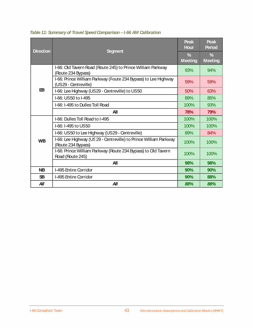
I-66 Consultant Team 43 Microsimulation Assumptions and Calibration Results (DRAFT)
Table 11: Summary of Travel Speed Comparison – I-66 AM Calibration
Direction Segment
PeakHour
PeakPeriod
%Meeting
%Meeting
EB
I-66: Old Tavern Road (Route 245) to Prince William Parkway(Route 234 Bypass) 93% 94%
I-66: Prince William Parkway (Route 234 Bypass) to Lee Highway(US 29 - Centreville) 59% 59%
I-66: Lee Highway (US 29 - Centreville) to US 50 50% 63%I-66: US 50 to I-495 89% 85%I-66: I-495 to Dulles Toll Road 100% 93%
All 78% 79%
WB
I-66: Dulles Toll Road to I-495 100% 100%I-66: I-495 to US 50 100% 100%I-66: US 50 to Lee Highway (US 29 - Centreville) 89% 84%I-66: Lee Highway (US 29 - Centreville) to Prince William Parkway(Route 234 Bypass) 100% 100%
I-66: Prince William Parkway (Route 234 Bypass) to Old TavernRoad (Route 245) 100% 100%
All 98% 98%NB I-495 Entire Corridor 90% 90%SB I-495 Entire Corridor 90% 88%All All 88% 88%

I-66 Consultant Team 44 Microsimulation Assumptions and Calibration Results (DRAFT)
Figure 27: Speed Diagrams – Comparison of INRIX Data and VISSIM Results – AM Period – I-66 Corridor EastboundDirection

I-66 Consultant Team 45 Microsimulation Assumptions and Calibration Results
PM Existing ModelThe PM model was calibrated using similar techniques described for the AM model.
TRAVEL TIME CALIBRATION RESULTS
Travel times produced from the VISSIM model were compared to field measures based on the criteriadescribed in previous sections. Figure 28 and Table 12 summarize the results for the westbounddirection for the following corridor segments:
· I-66 WB: Dulles Toll Road to I-495· I-66 WB: I-495 to US 50· I-66 WB: US 50 to Lee Highway (US 29 - Centreville)· I-66 WB: Lee Highway (US 29 - Centreville) to Prince William Parkway (Route 234 Bypass)· I-66 WB: Prince William Parkway (Route 234 Bypass) to Old Tavern Road (Route 245)
In Figure 28, calibration targets are depicted with high-low bars on field travel-time measures. As shownin this figure and on Table 12, calibration targets are met for all the general purpose lanes and HOVlanes for all segments, except for general purpose segment from US 50 to Lee Highway (US 29-Centreville). The travel time of the general purpose lanes for the entire corridor is within 1 percent ofthe field travel times and that of the HOV lanes is within 6 percent. In the eastbound direction, thedifference in the travel time for the entire corridor is within 1 percent.

I-66 Consultant Team 46 Microsimulation Assumptions and Calibration Results (DRAFT)
Figure 28: Travel Time Results – PM Combined Corridor Segments
Figure 29 and Figure 30, summarize the results for the entire corridor for every segment betweeninterchanges for both westbound and eastbound respectively. The figures show that there is a very closematch between the VISSIM travel times and the field travel times throughout the corridor in bothdirections for general purpose and HOV lanes.
0
200
400
600
800
1000
1200
1400
1600
I-66 WB: DullesToll Road to I-495
I-66 WB: I-495 toUS 50
I-66 WB: US 50 toUS 29 (Centreville)
I-66 WB: US 29(Centreville) to
Route 234 Bypass
I-66 WB: Route234 Bypass to Old
Tavern Road
Seco
nds
I-66 Westbound PM
VISSIM Increment - General Purpose
Field Increment - General Purpose
VISSIM Increment - HOV
Field Increment - HOV

I-66 Consultant Team 47 Microsimulation Assumptions and Calibration Results
Figure 29: Travel Time Results – PM Calibration – Westbound - All Corridor Segments
Figure 30: Travel Time Results – PM Calibration – Eastbound - All Corridor Segments
0
500
1000
1500
2000
2500
3000
3500
4000
I-66 WB: Route267 to Route 7
I-66 WB: Route7 to I-495
I-66 WB: I-495to Route 243
I-66 WB: Route243 to Route
123
I-66 WB: Route123 to US 50
I-66 WB: US 50to Fairfax
CountyParkway
I-66 WB: FairfaxCounty
Parkway toRoute 28
I-66 WB: Route28 to US 29(Centreville)
I-66 WB: US 29(Centreville) to
Route 234Business
I-66 WB: Route234 to Route234 Bypass
I-66 WB: Route234 Bypass to
US 29(Gainesville)
I-66 WB: US 29(Gainesville) to
US 15
I-66 WB: US 15to Old Tavern
Road
Seco
nds
I-66 Westbound PM
VISSIM Increment
Field Increment
VISSIM Increment - HOV
Field Increment - HOV
VISSIM Cumulative
Field Cumulative
VISSIM Cumulative - HOV
Field Cumulative - HOV

I-66 Consultant Team 48 Microsimulation Assumptions and Calibration Results (DRAFT)
0
500
1000
1500
2000
2500
I-66 EB: OldTavern Road to
US 15
I-66 EB: US 15 toUS 29
(Gainesville)
I-66 EB: US 29(Gainesville) to
Route 234 Bypass
I-66 EB: Route234 Bypass to
Route 234Business
I-66 EB: Route234 Business to
US 29(Centreville)
I-66 EB: US 29(Centreville) to
Route 28
I-66 EB: Route 28to Fairfax County
Parkway
I-66 EB: FairfaxCounty Parkway
to US 50
I-66 EB: US 50 toRoute 123
I-66 EB: Route123 to Route 243
I-66 EB: Route243 to I-495
I-66 EB: I-495 toRoute 7
Seco
nds
I-66 Eastbound PM
VISSIM Increment - General Purpose
Field Increment - General Purpose
VISSIM Cumulative - General Purpose
Field Cumulative - General Purpose

I-66 Consultant Team 49 Microsimulation Assumptions and Calibration Results (DRAFT)
Table 12: Summary of Travel Time Comparison – I-66 PM Westbound Calibration
SEGMENT
GENERAL PURPOSE HOVVISSIM
INCREMENT -GP
FIELD
INCREMENT
- GP
DIFFERENTIAL
(INCREMENT)
VISSIMINCREMENT -
HOV
FIELD
INCREMENT -HOV
DIFFERENTIAL
(INCREMENT)
I-66 WB: Dulles Toll Road to I-495 135 157 14% 132 146 9%I-66 WB: I-495 to US 50 1313 1246 5% 754 709 8%I-66 WB: US 50 to Lee Highway (US 29 -Centreville)
685 852 20% 420 390 8%
I-66 WB: Lee Highway (US 29 - Centreville) toPrince William Parkway (Route 234 Bypass)
631 600 5% 490 452 8%
I-66 WB: Prince William Parkway (Route 234Bypass) to Old Tavern Road (Route 245)
669 630 6% 667 627 6%
TOTAL (MINUTES) 57.2 58.1 1% 41.1 38.7 6%
ROUTE 28 TRAVEL TIME CALIBRATION RESULTS
Travel times produced from the VISSIM model were compared to field measures based on the criteriadescribed in previous sections. Figure 31 and Figure 32, as well as Table 13 and Table 14, summarize theresults for the northbound and southbound directions for the following corridor segments:
· Route 28 NB: US 29 to I-66· Route 28 NB: I-66 to Braddock Road/Walney Road· Route 28 NB: Braddock Road/Walney Road to EC Lawrence Park· Route 28 NB: EC Lawrence Park to Westfields Blvd Off-Ramp
· Route 28 SB: Westfields Blvd On-Ramp to EC Lawrence Park· Route 28 SB: EC Lawrence Park to Braddock Road/Walney Road· Route 28 SB: Braddock Road/Walney Road to I-66· Route 28 SB: I-66 to US 29
Since the total travel time along the Route 28 corridor, from US 29 to Westfields Boulevard is less than 7minutes, the target threshold for travel time segments is a differential of less than one minute. Asshown in Table 13 and Table 14, calibration targets are met for the Route 28 mainline through lanes forall the segments. The travel time to traverse the entire corridor, in the northbound and southbounddirections, is also within one minute of the field travel times.

I-66 Consultant Team 50 Microsimulation Assumptions and Calibration Results (DRAFT)
Figure 31: Route 28 Travel Time Results – PM Calibration – Southbound
Figure 32: Route 28 Travel Time Results – PM Calibration – Northbound
0
50
100
150
200
250
300
350
400
Route 28 SB: Westfields Blvd On-Ramp to EC Lawrence Park
Route 28 SB: EC Lawrence Park toBraddock Road/Walney Road
Route 28 SB: BraddockRoad/Walney Road to I-66
Route 28 SB: I-66 to US 29
Seco
nds
Route 28 Southbound PM Travel Time Comparison
VISSIM Increment
Field Increment
VISSIM Cumulative
Field Cumulative
0
50
100
150
200
250
Route 28 NB: US 29 to I-66 Route 28 NB: I-66 to BraddockRoad/Walney Road
Route 28 NB: BraddockRoad/Walney Road to EC Lawrence
Park
Route 28 NB: EC Lawrence Park toWestfields Blvd Off-Ramp
Seco
nds
Route 28 Northbound PM Travel Time Comparison
VISSIM IncrementField IncrementVISSIM CumulativeField Cumulative

I-66 Consultant Team 51 Microsimulation Assumptions and Calibration Results (DRAFT)
Table 13: Summary of Travel Time Comparison – Route 28 PM Southbound Calibration
SEGMENT
GENERAL PURPOSEVISSIM
INCREMENT
(SECONDS)
FIELD
INCREMENT
(SECONDS)
DIFFERENTIAL
(MINUTE)
Route 28 SB: Westfields Blvd On-Ramp to EC Lawrence Park 113 148 -0.58
Route 28 SB: EC Lawrence Park to Braddock Road/Walney Road 160 158 0.03
Route 28 SB: Braddock Road/Walney Road to I-66 48 37 0.18
Route 28 SB: I-66 to US 29 20 18 0.04
TOTAL (MINUTES) 5.69 6.02 -0.33
Table 14: Summary of Travel Time Comparison – Route 28 PM Northbound Calibration
SEGMENT
GENERAL PURPOSEVISSIM
INCREMENT
(SECONDS)
FIELD
INCREMENT
(SECONDS)
DIFFERENTIAL
(MINUTE)
Route 28 NB: US 29 to I-66 63 10 0.88
Route 28 NB: I-66 to Braddock Road/Walney Road 59 65 -0.10
Route 28 NB: Braddock Road/Walney Road to EC Lawrence Park 45 52 -0.12
Route 28 NB: EC Lawrence Park to Westfields Blvd Off-Ramp 41 41 0.00
TOTAL (MINUTES) 3.462 2.80 0.66
VOLUME CALIBRATION RESULTS
Throughput volumes produced by the VISSIM model were compared to balanced traffic counts based onthe criteria described in previous sections. Table 15 summarizes the comparison based on the GEHcriteria for the entire I-66 corridor, for combined segments for both eastbound and westbounddirection, for I-495 segments both for northbound and southbound directions, and for Route 28segments for northbound and southbound directions. The results are grouped by mainline segmentsand ramps. Table 15 also includes comparison results based on GEH criteria for all arterial approacheswithin the study area. As shown in this table, for the overall network, ramps, and intersectionapproaches all meet the target of 85 percent or more segments meeting the GEH criteria. The mainlinesegments are very near to the target, with 81 percent of segments meeting the GEH criteria.

I-66 Consultant Team 52 Microsimulation Assumptions and Calibration Results (DRAFT)
Table 15: Summary of Volume Comparison – I-66/I-495 PM Calibration
Section ID SegmentNumber of Locations Locations Meeting GEH Percent Meeting GEH
Mainline Ramps Overall Mainline Ramps Overall Mainline Ramps OverallOverall Study Area 209 259 468 169 249 419 81% 96% 90%
EB
1I-66: Old Tavern Road (Route 245) toPrince William Parkway (Route 234Bypass)
14 16 30 14 16 30 100% 100% 100%
2I-66: Prince William Parkway (Route 234Bypass) to Lee Highway (US 29 -Centreville)
15 14 29 15 14 29 100% 100% 100%
3 I-66: Lee Highway (US 29 - Centreville) toUS 50 14 21 35 13 20 33 93% 95% 94%
4 I-66: US 50 to I-495 15 30 45 12 30 42 80% 100% 93%5 I-66: I-495 to Dulles Toll Road 7 9 16 3 9 12 43% 100% 75%
Total: I-66 Eastbound 65 90 155 57 89 146 88% 99% 94%
WB
6 I-66: Dulles Toll Road to I-495 14 12 26 14 11 25 100% 92% 96%7 I-66: I-495 to US 50 15 23 38 10 22 32 67% 96% 84%
8 I-66: US 50 to Lee Highway (US 29 -Centreville) 13 20 33 13 17 30 100% 85% 91%
9I-66: Lee Highway (US 29 - Centreville) toPrince William Parkway (Route 234Bypass)
14 6 20 2 6 8 14% 100% 40%
10 I-66: Prince William Parkway (Route 234Bypass) to Old Tavern Road (Route 245) 15 11 26 15 11 26 100% 100% 100%
Total: I-66 Westbound 71 72 143 54 67 121 76% 93% 85%
NB 11 I-495 Entire Corridor 24 32 56 22 32 55 92% 100% 98%
SB 12 I-495 Entire Corridor 28 40 68 19 37 56 68% 93% 84%
NB 13 Route 28 Entire Corridor 10 13 23 10 12 22 100% 92% 96%
SB 14 Route 28 Entire Corridor 11 12 23 7 12 19 64% 100% 83%
Arterial Approaches 280 261 93%

I-66 Consultant Team 53 Microsimulation Assumptions and Calibration Results
Figure 33 below depicts the percentage of links meeting the GEH criteria as well as the volumedifference criteria (see targets in Table 5). Both cases meet the target of 85 percent or more linksmeeting the criteria.
Figure 33: Freeway Volume Results – PM Calibration – All Corridor Segments
Similar to the freeway volumes, intersection approach volumes were compared to traffic counts forboth GEH and volume difference criteria. Figure 34 illustrates the results for the PM peak hour. Asshown, 95 percent of approaches meet the GEH criteria while 92 percent meet the volume differentialcriteria.
Figure 34: Arterial Volume Results – PM Calibration – All Corridor Segments
121,85%
22,15%
Locations with GEH <5 Locations with GEH > 5
126,88%
17, 12%
Volume Difference Threshold Met
Volume Difference Threshold Not Met
265,95%
13,5%
Approaches with GEH <5
Approaches with GEH >5
257,92%
21,8%
Volume Differential: Threshold Met
Volume Differential: Threshold Not Met

I-66 Consultant Team 54 Microsimulation Assumptions and Calibration Results (DRAFT)
In addition, R-square plots were developed to test the correlation between VISSIM throughput and fieldcounts. Figure 35, Figure 36, and Figure 37 depict the results for the PM period for all freeway links,mainline segments, and ramp segments respectively. As shown in these figures, R-squared resultsranging between 0.97 and 0.99 confirm a good fit between model throughputs and field counts.
Figure 35: Freeway R-squared Plots – PM Period – All Corridor Segments
y = 0.9782x - 1.1724R² = 0.9886
0
1000
2000
3000
4000
5000
6000
7000
8000
9000
10000
0 1000 2000 3000 4000 5000 6000 7000 8000 9000 10000
VISS
IMTh
roug
hput
Balanced Count
All Freeway/Ramp Links

I-66 Consultant Team 55 Microsimulation Assumptions and Calibration Results (DRAFT)
Figure 36: Freeway R-squared Plots – PM Period – Mainline Segments
Figure 37: Freeway R-squared Plots – PM Period – Ramp Segments
y = 0.9737x + 24.504R² = 0.9702
0
1000
2000
3000
4000
5000
6000
7000
8000
9000
10000
0 1000 2000 3000 4000 5000 6000 7000 8000 9000 10000
VISS
IMTh
roug
hput
Balanced Count
Mainline Freeway Links
y = 0.9587x + 5.7299R² = 0.9864
0
500
1000
1500
2000
2500
3000
0 500 1000 1500 2000 2500 3000
VISS
IMTh
roug
hput
Balanced Count
Ramp Links

I-66 Consultant Team 56 Microsimulation Assumptions and Calibration Results (DRAFT)
SPEED CALIBRATION
Average Speeds were compared to INRIX speeds collected for similar days when traffic data wascollected in the field. Table 16 summarizes the results of this comparison. Based on the criteriadescribed in Table 6, while several segments closely match INRIX speeds, many others fall short. In thewestbound direction, 78 percent of the links meet the criteria with some segments between the DullesToll Road and Lee Highway (US 29) not meeting the speed criteria. However, in the eastbound I-66direction and along I-495 northbound, more than 90 percent of the links match the criteria. In thesouthbound direction of I-495, the criteria is met for the peak hour; however, for the peak period only,70 percent of the links meet the GEH criteria. INRIX data was not collected for Route 28, and thereforethis corridor is not included in the speed calibration. Variations on individual segments are expected forseveral reasons, the most important being the fact that INRIX data is less reliable than travel time fielddata thus it was used as a second or third tier in the calibration priority measures. INRIX data is anaverage speed of all lanes including auxiliary and declaration/acceleration lane speeds. In locationswhere there is a spill back of a ramp which mainly affects the exiting lanes, INRIX speeds will be lowerwhile the travel time speeds would be greater if they were conducted in lanes that were not affected bythe spill back.
BOTTLENECK LOCATIONS, LENGTH AND DURATION OF BACKUPS
Comparison of INRIX data with travel speeds measured in the model every half mile provided a veryuseful way for checking bottleneck locations as well as the extent and temporal distribution of mainlinequeues and overall congestion. Figure 38 depict the “heat” diagrams for the entire corridor for thewestbound direction in the PM period. As shown, there is a very reasonable match between INRIX andVISSIM results. It is important to note, that while this comparison provides a powerful way of checkingthe general validity of the model, other measures such as travel time and volumes are significantly morereliable and were given higher priority in the calibration process. Nevertheless, the results for the PMmodel are extremely close to what is observed from INRIX data in terms of specific bottleneck locations,length, and duration of backups. For Route 28, visual inspections of locations where congestionoriginated in the model were performed and verified against field observations. It is concluded that themodel reflects the congestion pattern on Route 28 corridor during the PM peak.

I-66 Consultant Team 57 Microsimulation Assumptions and Calibration Results (DRAFT)
Table 16: Summary of Travel Speed Comparison – PM Calibration
Direction Segment
PeakHour
PeakPeriod
%Meeting
%Meeting
EB
I-66: Old Tavern Road (Route 245) to Prince William Parkway(Route 234 Bypass) 100% 100%
I-66: Prince William Parkway (Route 234 Bypass) to Lee Highway(US 29 - Centreville) 100% 100%
I-66: Lee Highway (US 29 - Centreville) to US 50 88% 89%I-66: US 50 to I-495 77% 80%I-66: I-495 to Dulles Toll Road 44% 63%
All 90% 92%
WB
I-66: Dulles Toll Road to I-495 94% 90%I-66: I-495 to US 50 41% 39%I-66: US 50 to Lee Highway (US 29 - Centreville) 56% 65%I-66: Lee Highway (US 29 - Centreville) to Prince William Parkway(Route 234 Bypass) 80% 82%
I-66: Prince William Parkway (Route 234 Bypass) to Old TavernRoad (Route 245) 100% 100%
All 77% 78%NB I-495 Entire Corridor 90% 91%SB I-495 Entire Corridor 95% 70%All All 83% 85%

I-66 Consultant Team 58 Microsimulation Assumptions and Calibration Results (DRAFT)
Figure 38: Speed Diagrams – Comparison of INRIX Data and VISSIM Results – PM Period – I-66 CorridorWestbound Direction

I-66 Consultant Team 59 Microsimulation Assumptions and Calibration Results (DRAFT)
CONCLUSION
Based on the results obtained from the VISSIM AM and PM models and their comparison with field datafor all the calibration measures listed in previous sections, the I-66 Consultant Team concludes that themodels are reasonably calibrated to the standards and guidelines established by both VDOT and FHWAand, therefore, these models can be used as based models to develop future conditions for the analysis.