appendix b: acoustic modeling report - nsf eis/oeis nsf & usgs marine seismic research february...
TRANSCRIPT

APPENDIX B:
ACOUSTIC MODELING REPORT


APPENDIX B:
ACOUSTIC MODELING REPORT
Prepared by:
Scott A. Carr, Isabelle Gaboury, Marjo Laurinolli, Alex O. MacGillivray,
Stephen P. Turner, and Mikhail Zykov
JASCO Research Ltd. Halifax, Nova Scotia
Adam S. Frankel, William T. Ellison, and Kathleen Vigness-Raposa
Marine Acoustics, Inc. Arlington, Virginia
and
W. John Richardson, Mari A. Smultea, and William R. Koski
LGL Ltd., environmental research associates
King City, Ontario
Submitted to:
TEC Inc.
Annapolis, Maryland
February 2011

Acronyms and Abbreviations
2-D two-dimensional 3-D three-dimensional AASM Airgun Array Source Model AIM Acoustic Integration Model BC British Columbia bsf below the sea floor
DAA Detailed Analysis Area dB decibel(s)
dB re 1 Pa-1 m decibels referenced 1 microPascal
at 1 meter
dB re 1 Pa2 ∙ s decibels referenced 1 microPascal
squared second DSDP Deep Sea Drilling Project EIS Environmental Impact Statement ft foot/feet g/cm3 grams per cubic centimeter GDEM Generalized Digital Environmental Model GI generator injector
HF high-frequency hr hour(s) Hz hertz in3 cubic inches J Joule(s) kHz kilohertz km kilometer(s) L-DEO Lamont-Doherty Earth Observatory
LF low-frequency m meter(s) MAI Marine Acoustics, Inc.
MF mid-frequency min minute(s) MMO marine mammal observer MONM Marine Operations Noise Model ms millisecond(s) m/s meters per second
N North/Northern nmi nautical mile(s) NMFS National Marine Fisheries Service NSF National Science Foundation NW Northwestern ODP Ocean Drilling Program OEIS Overseas Environmental Impact Statement QAA Qualitative Analysis Area RAM Range Dependent Acoustic Model
RL received level rms root mean square R/V Research Vessel S South/Southern s second(s) SEL sound exposure level SL source level SPL sound pressure level
spp. species SW Southwestern TL transmission loss U.S. United States USGS U.S. Geological Survey W West/Western

Programmatic EIS/OEIS
NSF & USGS Marine Seismic Research February 2011
Appendix B:Acoustic Modeling Report B-i
Table of Contents
1 INTRODUCTION AND APPROACH ..................................................................................... 1
2 MAJOR FACTORS AFFECTING UNDERWATER SOUND PROPAGATION.................. 4
2.1 Spreading.................................................................................................................................... 4 2.2 Absorption .................................................................................................................................. 4 2.3 Refraction ................................................................................................................................... 4 2.4 Scattering.................................................................................................................................... 6 2.5 Bathymetry ................................................................................................................................. 6 2.6 Bottom Loss ............................................................................................................................... 7 2.7 Shear Waves ............................................................................................................................... 8
3 CLASSIFICATION OF OCEAN REGIONS ........................................................................... 9
3.1 Ocean Basin ................................................................................................................................ 9 3.2 Continental Shelf ........................................................................................................................ 9
4 SEISMIC SURVEY OVERVIEW .......................................................................................... 10
4.1 Airgun Operating Principles ...................................................................................................... 10 4.2 Airgun Array SLs ..................................................................................................................... 11
5 MODELING METHODOLOGY: RECEIVED SOUND LEVELS ..................................... 13
5.1 Airgun Array Source Model (AASM) ....................................................................................... 13 5.1.1 Research Vessel Marcus G. Langseth (Langseth) Airgun Arrays ................................. 14
5.2 Sound Propagation Model: MONM .......................................................................................... 17 5.2.1 Estimating 90% rms SPL from SEL ............................................................................ 17 5.2.2 M-Weighting for Marine Mammal Hearing Abilities................................................... 18
6 MONM PARAMETERS ........................................................................................................ 20
6.1 Survey Source Locations – DAAs ............................................................................................. 20 6.2 Sound Speed Profiles ................................................................................................................ 20 6.3 Model Receiver Depths ............................................................................................................. 21 6.4 Bathymetry and Acoustic Environment of DAAs ...................................................................... 22
6.4.1 S California ................................................................................................................ 22 6.4.2 Caribbean ................................................................................................................... 22 6.4.3 Galapagos Ridge ......................................................................................................... 23 6.4.4 W Gulf of Alaska........................................................................................................ 23 6.4.5 NW Atlantic ............................................................................................................... 24
6.5 Acoustic Environment of QAAs ................................................................................................ 25 6.5.1 Mid-Atlantic Ridge ..................................................................................................... 26 6.5.2 North Atlantic/Iceland (N Atlantic/Iceland)................................................................. 27 6.5.3 Mariana Islands (Marianas) ......................................................................................... 27 6.5.4 Sub-Antarctic ............................................................................................................. 27 6.5.5 Western India (W India) ............................................................................................. 27 6.5.6 Western Australia (W Australia) ................................................................................. 27 6.5.7 Southwest Atlantic Ocean (SW Atlantic) .................................................................... 28 6.5.8 British Columbia Coast (BC Coast) ............................................................................ 28
7 ACOUSTIC INTEGRATION MODEL (AIM) ...................................................................... 29
7.1 Rationale .................................................................................................................................. 29 7.2 Introduction to AIM .................................................................................................................. 30 7.3 Programmatic EIS/OEIS-Specific Modeling Methods ............................................................... 30 7.4 Data Convolution to Create Animat Exposure Histories ............................................................ 31

Programmatic EIS/OEIS
NSF & USGS Marine Seismic Research February 2011
B-ii Appendix B: Acoustic Modeling Report
7.5 Simulation of Monitoring and Mitigation .................................................................................. 32 7.6 Numbers of Mammals Exposed................................................................................................. 37 7.7 Marine Mammal Density Values ............................................................................................... 38
7.7.1 S California ................................................................................................................ 38 7.7.2 Caribbean ................................................................................................................... 38 7.7.3 Galapagos Ridge ......................................................................................................... 38 7.7.4 W Gulf of Alaska........................................................................................................ 38 7.7.5 NW Atlantic ............................................................................................................... 38
8 RESULTS ................................................................................................................................ 39
8.1 Sound Propagation Modeling – MONM .................................................................................... 39 8.1.1 S California ................................................................................................................ 40 8.1.2 Caribbean ................................................................................................................... 40 8.1.3 Galapagos Ridge ......................................................................................................... 41 8.1.4 W Gulf of Alaska........................................................................................................ 41 8.1.5 NW Atlantic ............................................................................................................... 42
8.2 SELs and 90% RMS SPLs ........................................................................................................ 42 8.3 Comparison with Free-field Models .......................................................................................... 43
8.3.1 TL Estimates .............................................................................................................. 43 8.3.2 Near-field vs. Far-field Estimates ................................................................................ 44
8.4 Marine Mammal Exposure Modeling – AIM ............................................................................. 44 8.4.1 S California ................................................................................................................ 46 8.4.3 Caribbean ................................................................................................................... 49 8.4.4 Galapagos Ridge ......................................................................................................... 52 8.4.5 W Gulf of Alaska........................................................................................................ 55 8.4.6 NW Atlantic ............................................................................................................... 58
10 LITERATURE CITED ........................................................................................................... 61
ANNEX 1: FAR-FIELD SL COMPUTATION .............................................................................. 67
ANNEX 2: AIRGUN ARRAY 1/3-OCTAVE BAND SLS ............................................................... 69
ANNEX 3: SOURCE LOCATIONS AND STUDY AREAS .......................................................... 75
ANNEX 4: MARINE MAMMAL SPECIES AND ASSOCIATED DENSITIES AND
ANIMAT DEPTH RESTRICTIONS INCLUDED IN AIM MODELING ................ 81
ANNEX 5: NOISE MAPS ............................................................................................................... 85
ANNEX 6: PREDICTED RANGES TO VARIOUS RLS .............................................................. 99

Programmatic EIS/OEIS
NSF & USGS Marine Seismic Research February 2011
Appendix B:Acoustic Modeling Report B-iii
List of Tables
Table B-1. Descriptions of R/V Langseth Standard Airgun Array Configurations................................... 15
Table B-2. Marine Mammal Functional Hearing Groups and Associated Auditory Bandwidths .............. 19
Table B-3. Source Coordinates and Array Axis Orientation ................................................................... 20
Table B-4. Injury and Behavior Exposure Criteria for Cetaceans and Pinnipeds ..................................... 29
Table B-5. Summary of Modeled Marine Mammal Level A Exposure Criteria Radii for DAAs ............. 32
Table B-6. Assumed P(detect) Values for Different Species................................................................... 33
Table B-7. Nominal Example of Exposure Calculation .......................................................................... 37
Table B-8. Summary of Predicted Marine Mammal Exposure Criteria Radii for the S California Sites ... 40
Table B-9. Summary of Predicted Marine Mammal Exposure Criteria Radii for the Caribbean Sites ...... 40
Table B-10. Summary of Predicted Marine Mammal Exposure Criteria Radii for the Galapagos
Ridge Sites .................................................................................................................................... 41
Table B-11. Summary of Predicted Marine Mammal Exposure Criteria Radii for the W Gulf of
Alaska Sites ................................................................................................................................... 41
Table B-12. Summary of Predicted Marine Mammal Exposure Criteria Radii for the NW Atlantic
Sites .............................................................................................................................................. 42
Table B-13. Real World Exposure Predictions for S California Site under Alternatives A and B ............ 48
Table B-14. Real World Exposure Predictions for the Caribbean Site under Alternatives A and B .......... 51
Table B-15. Real World Exposure Predictions for the Galapagos Ridge Site under Alternatives A
and B ............................................................................................................................................. 54
Table B-16. Real World Exposure Predictions for the W Gulf of Alaska Site under Alternatives A
and B ............................................................................................................................................. 57
Table B-17. Real World Exposure Predictions for the NW Atlantic Site under Alternatives A and B ...... 60
List of Figures
B-1. Generic Sound Speed Profiles with Some Common Terms Depicted ................................................ 5
B-2. Sensitivity of Propagation to Sound Speed ....................................................................................... 6
B-3. Examples of Estimates of Bottom Loss Curves ................................................................................ 7
B-4. Overpressure Signature for a Single Airgun, Showing the Primary Peak and the Bubble Pulse ....... 11
B-5. Diagram of R/V Langseth Standard 1,650 in3 Subarray Design for 2-D and 3-D Reflection or
Refraction Surveys ........................................................................................................................ 15
B-6. Computed Broadside and Endfire Overpressure Signatures, with Associated Frequency Spectra, for
R/V Langseth Airgun Arrays based on AASM ............................................................................... 16
B-7. Plots of Sound Speed Profiles vs. Depth from the GDEM Database for Each Modeling Site ........... 21

Programmatic EIS/OEIS
NSF & USGS Marine Seismic Research February 2011
B-iv Appendix B: Acoustic Modeling Report
B-8. Exemplary QAAs .......................................................................................................................... 25
B-9. Plots of Sound Speed Profiles vs. Depth from the GDEM Database for Proposed Exemplary
QAAs and Seasons ........................................................................................................................ 26
B-10. Illustration of Pressure-based Exposure or ―Take‖ Methodology (not to scale) ............................. 30
B-11. Example of Decreasing and Increasing Range between a Source Vessel and a Single Whale
Animat over Time, in Relation to the Mitigation Distance (red line) ............................................ 34
B-12. Time History of Predicted RL of the Whale Animat in Figure B-11 .............................................. 35
B-13. Ping-o-gram of First 2,500 Animats over 270 Minutes ................................................................. 36
B-14. Ping-o-gram of First 2,500 Animats over 270 Minutes but with Successful Mitigation
Implemented from Minute 130 to Minute 160 .............................................................................. 36
B-15. Stylized Diagram Showing Approximate Regions of Applicability of the MONM and
Free-field Models........................................................................................................................ 43
B-16. Distribution of Modeled Sound Exposures for Common Dolphin in the S California Site ............. 46
B-17. Distribution of Modeled Sound Exposures for California Sea Lion in the S California Site ........... 47
B-18. Distribution of Modeled Sound Exposures for Bottlenose Dolphin in the Caribbean Site .............. 49
B-19. Distribution of Modeled Sound Exposures for Pantropical Spotted Dolphin in the Caribbean
Site ............................................................................................................................................. 50
B-20. Distribution of Modeled Sound Exposures for Bryde‘s Whale in the Galapagos Ridge Site .......... 52
B-21. Distribution of Modeled Sound Exposures for Pantropical Spotted Dolphin in the Galapagos
Ridge Site ................................................................................................................................... 53
B-22. Distribution of Modeled Sound Exposures for Fin Whale in the W Gulf of Alaska Site ................ 55
B-23. Distribution of Modeled Sound Exposures for Steller‘s Sea Lion in the W Gulf of Alaska Site ..... 56
B-24. Distribution of Modeled Sound Exposures for Bottlenose Dolphin in the NW Atlantic Site .......... 58
B-25. Distribution of Modeled Sound Exposures for Sperm Whale in the NW Atlantic Site ................... 59
List of Figures – Annex 1
A1-1. Plan View Diagram of the Far-field Summation Geometry for an Airgun Array ........................... 67
List of Figures – Annex 2
A2-1. Directionality of the Airgun Array Source Levels (dB re μPa2 ∙ s) (R/V Langseth 2-D
Reflection, 2 x 1, 650 in3, 6 m tow depth) .................................................................................... 69
A2-2. Directionality of the Airgun Array Source Levels (dB re μPa2 ∙ s) (R/V Langseth 2-D
Reflection, 4 x 1, 650 in3, 6 m tow depth) .................................................................................... 70
A2-3. Directionality of the Airgun Array Source Levels (dB re μPa2 ∙ s) (R/V Langseth 2-D
Refraction, 4 x 1, 650 in3, 12 m tow depth).................................................................................. 71

Programmatic EIS/OEIS
NSF & USGS Marine Seismic Research February 2011
Appendix B:Acoustic Modeling Report B-v
A2-4. Directionality of the Airgun Array Source Levels (dB μPa2 ∙ s) (R/V Langseth 2-D High
Resolution, 2 x GI, 2.5 m tow depth) ........................................................................................... 72
A2-5. Directionality of the Airgun Array Source Levels (dB μPa2 ∙ s) (R/V Langseth 3-D High
Resolution, 2 x GI, 2.5 m tow depth) ........................................................................................... 73
List of Figures – Annex 3
A3-1. Locations of S California Modeling Sites ..................................................................................... 75
A3-2. Locations of Caribbean Modeling Sites ........................................................................................ 76
A3-3. Locations of Galapagos Ridge Modeling Sites ............................................................................. 77
A3-4. Locations of W Gulf of Alaska Modeling Sites ............................................................................ 78
A3-5. Locations of NW Atlantic Modeling Sites .................................................................................... 79
List of Tables – Annex 4
A4-1. Species and Densities Modeled at the Caribbean Site ................................................................... 81
A4-2. Species and Densities Modeled at the NW Atlantic Site ............................................................... 82
A4-3. Species and Densities Modeled at the Galapagos Ridge Site ......................................................... 82
A4-4. Species and Densities Modeled at the S California Site ................................................................ 83
A4-5. Species and Densities Modeled at the W Gulf of Alaska Site........................................................ 84
List of Figures – Annex 5
A5-1. Predicted SELs for S California Modeling Sites ........................................................................... 86
A5-2. Predicted SELs for S California Modeling Sites (zoomed-in from Figure A5-1) ........................... 87
A5-3. Predicted SELs for Caribbean Modeling Sites .............................................................................. 88
A5-4. Predicted SELs for Caribbean modeling sites (zoomed-in from Figure A5-3) ............................... 89
A5-5. Predicted SELs for Galapagos Ridge Modeling Sites ................................................................... 90
A5-6. Predicted SELs for Galapagos Ridge Modeling Sites (zoomed-in from Figure A5-5) ................... 91
A5-7. Predicted SELs for W Gulf of Alaska Modeling Sites 1 and 3 ...................................................... 92
A5-8. Predicted SELs for W Gulf of Alaska Modeling Site 2 ................................................................. 93
A5-9. Predicted SELs for W Gulf of Alaska Modeling Sites (zoomed-in from Figure A5-7 and
Figure A5-8 ................................................................................................................................. 94
A5-10. Predicted SELs for NW Atlantic Modeling Sites ........................................................................ 95
A5-11. Predicted SELs for NW Atlantic Modeling Sites (zoomed in from Figure A5-10)....................... 96
A5-13. Predicted SELs for Caribbean Site #2 (deep water), for Transects in the Aft Endfire (middle
panel) and Port Broadside (right panel) Directions .................................................................... 97

Programmatic EIS/OEIS
NSF & USGS Marine Seismic Research February 2011
B-vi Appendix B: Acoustic Modeling Report
A5-14. Predicted SELs for Caribbean Site #3 (slope), for Transects in the Forward Endfire (2nd
panel),
Aft Endfire (3rd
panel), and Starboard Broadside (4th panel) Directions ...................................... 98
List of Tables – Annex 6
A6-1. Predicted Maximum Marine Mammal Exposure Criteria Radii at the S California Sites ............... 99
A6-2. Predicted Maximum Marine Mammal Exposure Criteria Radii at the Caribbean Sites ................ 100
A6-3. Predicted Maximum Marine Mammal Exposure Criteria Radii at the Galapagos Ridge Sites ...... 100
A6-4. Predicted Maximum Marine Mammal Exposure Criteria Radii at the W Gulf of Alaska Sites ..... 101
A6-5. Predicted Maximum Marine Mammal Exposure Criteria Radii at the NW Atlantic Sites ............ 101

Programmatic EIS/OEIS
NSF & USGS Marine Seismic Research February 2011
Appendix B:Acoustic Modeling Report B-1
1 Introduction and Approach
This report provides technical information in support of the Programmatic Environmental Impact Statement/Overseas EIS (EIS/OEIS) prepared by the National Science Foundation (NSF) and the U.S. Geological Survey (USGS) concerning their marine seismic research operations. In particular, this report
describes the procedures used to estimate the airgun sound fields that would occur around the seismic
vessel during five exemplary seismic surveys and the numbers of marine mammals that might be exposed
to specified levels of underwater sound during those surveys.
The five exemplary cruises analyzed here are within five Detailed Analysis Areas (DAAs) that are analyzed in the EIS/OEIS for potential impacts on the human and natural environment with
implementation of marine seismic surveys funded by NSF or conducted by the USGS. The five DAAs consist of the Western Gulf of Alaska (W Gulf of Alaska), Southern California (S California), Galapagos
Ridge, Caribbean Sea (Caribbean), and northwest Atlantic Ocean (NW Atlantic) (see Annex 3 to this
report). These areas include a wide variety of water depths, sound propagation conditions, and types of
marine mammals. Also, the five exemplary seismic surveys involve a wide variety of airgun sources, ranging from a small two generator injector (GI)-gun configuration to a large 36-airgun configuration.
The EIS/OEIS also considers, in a qualitative way, eight additional exemplary cruises to other geographic
regions or qualitative analysis areas (QAAs). However, those are not considered in this technical analysis of the anticipated sound fields and numbers of marine mammals exposed to specified sound levels.
To estimate the sound fields expected to exist during the surveys in the five DAAs, two quantitative acoustic models were applied in sequence. First, for each configuration of airguns planned for use in one or more of the DAAs, an Airgun Array Source Model (AASM) was used to predict the amount
of sound that would be projected in each direction. This model takes account of the specific sizes and
positions of the individual airguns relative to one another, along with the depths of the airguns below the
water surface. The model predicts the sound output, in each direction, by ⅓-octave frequency band (see Section 5.1 for details).
The second acoustic model that was used is the Marine Operations Noise Model (MONM),
described in Section 5.2. This model predicts the received levels (RLs) of airgun sound as a function of bearing, distance, and depth in the water column. This model was run for two to four representative
locations within each of the five DAAs. The MONM takes account of the frequency-specific source levels
predicted by the AASM for the particular airgun configuration to be used in each DAA. It also takes account of the best available site-specific information about environmental factors that would affect the
propagation and attenuation of that sound as it travels outward from the airgun array. These include
bathymetry, sub-bottom conditions, and the sound velocity profile of the water column (see Section 6).
MONM predicted the received sound field around the various representative locations for each ⅓-octave band. The predicted values were, for each location in the sound field, the received energy level for an
individual pulse, in decibels reference 1 microPascal squared second (dB re 1 Pa2 ∙ s). This energy value
is commonly referred to as the sound exposure level (SEL).
Since the mid-1990s, the U.S. National Marine Fisheries Service (NMFS) has specified that
marine mammals should not be exposed to pulsed sounds with RLs exceeding 180 or 190 dB re 1 Pa (rms). Here rms, or root mean square, refers to a particular method of measuring the average sound pressure over the approximate duration of an individual sound pulse. Since 2000, the ―do not exceed‖
levels have been specified as 180 dB re 1 Pa (rms) for cetaceans and 190 dB (rms) for pinnipeds (NMFS
2000). NMFS also considers that both cetaceans and pinnipeds exposed to levels ≥160 dB re 1 Pa (rms) may be disturbed.
The 180- and 190-dB (rms) ―do-not-exceed‖ criteria were determined before there was any specific information about the RLs of underwater sound that would cause temporary or permanent hearing

Programmatic EIS/OEIS
NSF & USGS Marine Seismic Research February 2011
B-2 Appendix B: Acoustic Modeling Report
damage in marine mammals. Subsequently, data on RLs that cause the onset of temporary threshold shift
(TTS) have been measured for certain toothed whales and pinnipeds (Kastak et al. 1999; Finneran et al. 2002, 2005). There are no specific data concerning the levels of underwater sound necessary to cause
permanent hearing damage (permanent threshold shift or PTS) in any species of marine mammal.
However, data from terrestrial mammals provide a basis for estimating the difference between the
(unmeasured) PTS thresholds and the measured TTS thresholds. A group of specialists in marine mammal acoustics, the ―Noise Criteria Group‖, has recently recommended new criteria, based on current scientific
knowledge, to replace the somewhat arbitrary 180 and 190 dB (rms) ―do-not-exceed‖ criteria. The
primary measure of sound used in the new criteria is the received sound energy, not just in the single strongest pulse, but accumulated over time. On that basis, the received sound levels above which some
auditory damage (PTS) might occur were determined by the Noise Criteria Group to be 198 dB re 1
Pa2 ∙ sec for any cetacean, and 186 dB re 1 Pa
2 ∙ sec for pinnipeds.
A further recommendation from the Noise Criteria Group is that allowance should be given to the
differential frequency responsiveness of various marine mammal groups and use what are known as M-weighted curves (Southall et al. 2007). This is important when considering airgun sounds: the energy in
airgun sounds is predominantly at low frequencies (below 500 hertz [Hz]), with diminishing amounts of
energy at progressively higher frequencies (Greene and Richardson 1988; Goold and Fish 1998). Baleen whales (mysticetes) are most sensitive to low-frequency sounds, and not very sensitive to high-frequency
sounds. On the other hand, odontocetes or toothed whales (including dolphins and porpoises) are quite
insensitive to low frequencies but very sensitive to high frequencies (Richardson et al. 1995). As
compared with other odontocetes, porpoises, river dolphins, and the Southern-Hemisphere genus Cephalorhynchus are even less sensitive to low frequencies than are other odontocetes. Pinnipeds are
intermediate between baleen and toothed whales. However, the recommendations from the Noise Criteria
Group have not yet been adopted by NMFS. Therefore, the analysis considered both M-weighted and unweighted (flat) RLs, and produced take estimates for both.
The Noise Criteria Group has proposed that, in calculating the effective SELs, frequency weighting functions should be applied (Southall et al. 2007). These so-called ―M-weighting‖ curves de-emphasize the high-frequency energy when dealing with baleen whales, and de-emphasize the low-
frequency energy when dealing with odontocetes. For pinnipeds, there is some de-emphasis of both the
low-and high-frequency energy, but the low frequencies are weighted more heavily than for odontocetes,
and the high frequencies are weighted more heavily than for mysticetes. The shapes of the M-weighting curves are similar to those of C-weighting curves that are widely used when considering effects of strong
pulsed sounds on human hearing. However, the M-weighting curves are shifted downward in frequency
for baleen whales and upward in frequency for toothed whales. In this analysis, the M-weighting curves were applied when estimating effective received energy levels. This was done by applying the M-weights
to MONM‘s estimates of the received energy levels in each ⅓-octave frequency band before
accumulating across bands to derive the overall received energy level.
To estimate the number of marine mammals of each species or species-group that would receive various amounts of sound energy, we applied the Acoustic Integration Model (AIM) developed by Marine
Acoustics Inc. (MAI) (Frankel et al. 2002). For each species or group in each DAA, AIM simulated the
three-dimensional (3-D) motion of the mammal population, taking account of existing knowledge of diving and swimming behavior. At short intervals of time, AIM predicted the bearing and distance of each
simulated animal from the (moving) seismic source, along with the depth of the animal. The expected RL
of airgun sound at that bearing, distance and depth was determined from JASCO‘s MONM results for the most representative acoustic modeling site. For each simulated animal, the time-history of received
energy levels was predicted for the full duration of the simulated seismic cruise. From these individual
time-histories, the total received sound energy was determined for the 24-hour (hr) period centered on the
time when the received sound was strongest. By considering all the simulated animals, AIM could then
Programmatic EIS/OEIS
NSF & USGS Marine Seismic Research February 2011
Appendix B:Acoustic Modeling Report B-3
estimate how many marine mammals would, over the course of the seismic survey, receive any specified
amount of sound energy in at least one 24-hr period.
A further feature built into the AIM process was to take account of mitigation strategies. Implementation of either Alternative A or Alternative B involved shutting down the airguns if a cetacean
or pinniped is detected within the 180- or 190-dB (rms) radius, respectively (a mitigation strategy that has
been used by NSF in the past.). The airguns were assumed to remain off for a specified period after each shutdown, during which time none of the simulated mammals would be receiving airgun sound.
The 180- and 190-dB (rms) radii used in simulating the mitigation process were derived from the
MONM modeling with the additional assumption that, for airgun pulses, rms RLs measured in dB re 1
Pa average about 10 dB higher than SEL (energy) values in dB re 1 Pa2 ∙ s (Greene 1997; McCauley et
al. 1998; Blackwell et al. 2006; MacGillivray and Hannay 2007). Also, the 180- and 190-dB (rms) radii
used as assumed mitigation distances included M-weighting, so were smaller for pinnipeds and especially
for odontocetes than for baleen whales. These factors caused the 180- and 190-dB (rms) radii to vary
widely depending on airgun configuration, water depth, and type of animal.
This report and its Annexes describe the acoustic modeling and AIM simulation processes in some detail, and present the results for the five DAAs. The results are used in the EIS/OEIS to help assess
the potential impacts on marine mammals of NSF-funded or USGS marine seismic research.
Programmatic EIS/OEIS
NSF & USGS Marine Seismic Research February 2011
B-4 Appendix B: Acoustic Modeling Report
2 Major Factors Affecting Underwater Sound Propagation
Knowledge of the properties of the surrounding environment is necessary for the study of underwater acoustics. Some of the factors that affect sound propagation in the ocean, such as spreading and directivity, are well understood and predictable. However, scattering of sound from the surface and
bottom boundaries and from other objects is difficult to quantify (due to its dependence on fine-scale
features of the local environment), and unfortunately scattering is extremely important in characterizing
and understanding the sound field. These factors need to be taken into account when using a numerical model to predict sound propagation losses and RLs in water.
2.1 Spreading
Spreading refers to the geometric distribution of sound energy as it leaves a source. For sound propagating from an omnidirectional source in the absence of boundaries, the received sound level
decreases with the square of the distance from the source as the transmitted energy is distributed over the
expanding spherical wave front. The transmission loss (TL) in decibels (dB) from spherical spreading in this scenario is 20 log10 R (where R = range). This formula can be applied at short range from an
omnidirectional source. However, as R increases, boundary interactions begin to focus the sound (e.g., by
reflection from the surface and sea floor) and the factor 20 changes to 10 or even 5. The situation is also more complex for a directional source (e.g., an airgun), for which spreading may occur primarily in a few
preferred directions.
2.2 Absorption
As sound waves propagate, they interact at a molecular level with the constituents of sea water through a range of mechanisms, resulting in absorption of sound energy (Francois and Garrison 1982a, b;
Medwin 2005). This occurs even in completely particulate-free waters, and is in addition to scattering that may occur from objects such as zooplankton or suspended sediments (see Section 2.4). The absorption of
sound energy by water contributes to the TL linearly with range and is given by an attenuation coefficient
in units of decibels per kilometer (dB/km). This absorption coefficient is computed from empirical
equations and increases with the square of frequency. For example, for typical open-ocean values (temperature of 10°C, pH of 8.0, and a salinity of 35 practical salinity units [psu]), the equations
presented by Francois and Garrison (1982a, b) yield the following values for attenuation near the sea
surface: 0.001 dB/km at 100 Hz, 0.06 dB/km at 1 kilohertz (kHz), 0.96 dB/km at 10 kHz, and 33.6 dB/km at 100 kHz. Thus, low frequencies are favored for long-range propagation.
2.3 Refraction
Refraction refers to a change of direction in a propagating wave due to spatial variations in sound speed within the medium. As a wave travels across a sound speed interface or gradient, portions of the
wave front travel at different speeds, resulting in bending of the ray path (Medwin 2005). By affecting
travel paths within the medium, refraction controls the angle of arrival of the sound at a receiver as well
as the angle of incidence upon boundaries (e.g., the sea floor).
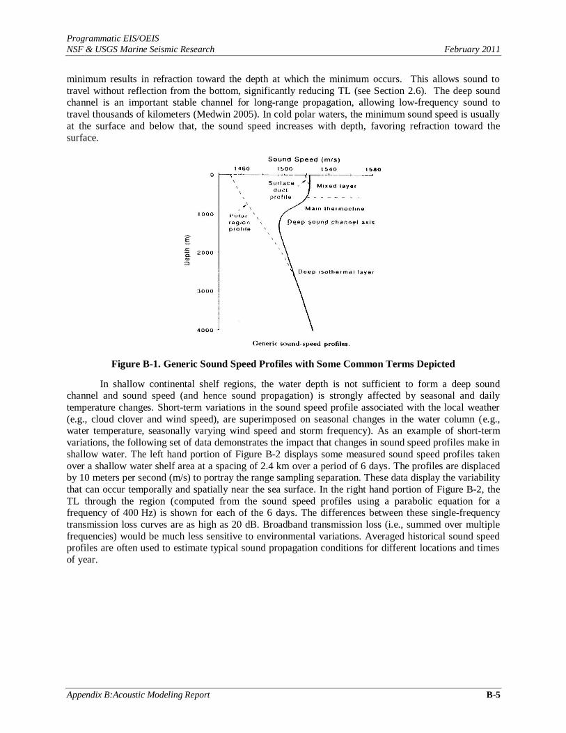
The fundamental requirement for refraction calculations is knowledge of the sound speed profile. Figure B-1 shows a generic profile of sound speed as a function of depth, as might occur in
temperate waters. Because of the strong influence of temperature, sound speed varies the most near the surface both seasonally and daily. If the wind has mixed the water to a constant temperature near the
surface, then the increase in speed with depth (pressure) will result in upward refraction of propagating
sound waves. Sound will tend to be channeled in the near-surface layer, referred to as a surface duct, as it
is repeatedly reflected downward from the air-sea interface and refracted upward by the positive sound speed gradient (Medwin 2005). In the thermocline, temperature and sound speed decline, but below this,
the temperature is constant and sound speed begins to increase again with depth. The sound speed
Programmatic EIS/OEIS
NSF & USGS Marine Seismic Research February 2011
Appendix B:Acoustic Modeling Report B-5
minimum results in refraction toward the depth at which the minimum occurs. This allows sound to
travel without reflection from the bottom, significantly reducing TL (see Section 2.6). The deep sound channel is an important stable channel for long-range propagation, allowing low-frequency sound to
travel thousands of kilometers (Medwin 2005). In cold polar waters, the minimum sound speed is usually
at the surface and below that, the sound speed increases with depth, favoring refraction toward the
surface.
Figure B-1. Generic Sound Speed Profiles with Some Common Terms Depicted
In shallow continental shelf regions, the water depth is not sufficient to form a deep sound channel and sound speed (and hence sound propagation) is strongly affected by seasonal and daily
temperature changes. Short-term variations in the sound speed profile associated with the local weather
(e.g., cloud clover and wind speed), are superimposed on seasonal changes in the water column (e.g., water temperature, seasonally varying wind speed and storm frequency). As an example of short-term
variations, the following set of data demonstrates the impact that changes in sound speed profiles make in
shallow water. The left hand portion of Figure B-2 displays some measured sound speed profiles taken
over a shallow water shelf area at a spacing of 2.4 km over a period of 6 days. The profiles are displaced by 10 meters per second (m/s) to portray the range sampling separation. These data display the variability
that can occur temporally and spatially near the sea surface. In the right hand portion of Figure B-2, the
TL through the region (computed from the sound speed profiles using a parabolic equation for a frequency of 400 Hz) is shown for each of the 6 days. The differences between these single-frequency
transmission loss curves are as high as 20 dB. Broadband transmission loss (i.e., summed over multiple
frequencies) would be much less sensitive to environmental variations. Averaged historical sound speed profiles are often used to estimate typical sound propagation conditions for different locations and times
of year.

Programmatic EIS/OEIS
NSF & USGS Marine Seismic Research February 2011
B-6 Appendix B: Acoustic Modeling Report
Figure B-2. Sensitivity of Propagation to Sound Speed Left: Measured shallow water profiles taken over a 6-day period on a spatial sampling grid 2.4 km apart. Sound
speed (in m/s) is shown on the x-axis and depth (in m) on the y-axis. On each day‘s graph, the profiles are
offset by 10 m/s to represent the sample spacing.
Right: 400 Hz TL as a function of range computed for each day of the 6-day experiment (McCammon 2000).
2.4 Scattering
Scattering is a general term that covers several types of interactions arising from the interaction of a propagating wave front with inhomogeneities in the medium (e.g., suspended particulates, bubbles, buried objects, air-sea or sea-sediment interfaces). Sound energy arriving at an object may bend around it
(diffraction) and/or be scattered back toward the source (backscattering) or in some other direction. For
sound incident upon an interface such as the sea floor, some of the energy is reflected, while some of the
energy is transmitted across the interface (with refraction); see also Section 2.6 below. For complex objects (e.g., a rough sea floor), the nature of these interactions can be quite complicated, as individual
portions of a wave front are scattered differently (Medwin 2005). However, if the acoustic wavelength is
much greater than the scale of the seabed non-uniformities (as is most often the case for low-frequency sounds) then the effect of scattering on propagation loss is negligible.
2.5 Bathymetry
Water depth is very influential on sound propagation, particularly at frequencies less than a few kilohertz. In shallow water (less than ~100m depth) propagation loss is dominated by reflection and
scattering of sound from the seabed. In deep water (greater than ~1 km depth) sound propagation is
dominated by refraction in the water column. At intermediate depths, propagation loss is influenced by a
combination of these two factors.
As discussed above, sound arriving at an interface such as the sea floor is both reflected from the interface and transmitted into the lower medium with refraction. The proportion of the sound energy that
is reflected or refracted depends both on the sound speed in each medium and on the angle of incidence upon the interface, with greater reflection for shallower angles of incidence (Medwin 2005). Thus, water
0 5 10 15 20 25 30 35 40 45 -130
-120
-110
-100
-90
-80
-70
-60
-50
-40
-30
Range (km)
TL (dB)
TL each day

Programmatic EIS/OEIS
NSF & USGS Marine Seismic Research February 2011
Appendix B:Acoustic Modeling Report B-7
depth has a very large influence on underwater sound propagation, especially at low to mid frequencies
(less than a few kilohertz) where scattering losses are low.
2.6 Bottom Loss
Considering a sound pulse that has traveled from a source to a receiver (where both are above the bottom) by reflecting from the bottom, bottom loss refers to the decrease in signal strength that occurs
from the bottom reflection. Computation of this value in real life is difficult, due to the complexity of sound propagation at the water-sediment interface. Sound energy arriving at the sea floor may be
reflected, scattered in many different directions by surface roughness, or transmitted into the sea floor.
Transmitted sound is refracted and undergoes attenuation within the sediments. Furthermore, the same processes of reflection and refraction may occur at the interfaces between different sediment layers,
possibly returning some of the sound energy to the water column.
Because sound penetrates sediments readily, especially at low frequencies (Clay and Medwin 1977; Hamilton 1980), knowledge of the bottom loss is a critical factor in modeling sound transmission.
This requires information on the composition and internal structure of the sediments. However, unlike
sound speed or bathymetry, there are no easy ways to measure or compute this quantity. Specialized
sampling is generally employed to characterize the bottom at different grazing angles and frequencies to try to discover its composition and layering. A great deal of effort has been made recently to characterize
sediments by their physical properties of density, speed, and attenuation (both compressional and shear)
and to provide theoretical calculations that will convert these physical quantities (called geoacoustic parameters) into acoustic bottom loss. However the efforts have been only partially successful and this is
still an ongoing area of research.
In Figure B-3, theoretical estimates for bottom loss from mud (left) and sand (right) are shown. Note the vertical scale change between the figures. The mud bottom can be over twice as lossy as the sand
due to greater transmission of sound into the sediments, reflecting differences in the speed of sound
within the two sediment types (Hamilton 1980). Furthermore, there are differences between hard packed
sand, sand and shell, and loose sand, as well as many other sediment types not shown in these figures. Bottom loss is a complex and only partly understood phenomenon.
Figure B-3. Examples of Estimates of Bottom Loss Curves
Note: The left curves are for mud bottoms while the right curves are for sand.

Programmatic EIS/OEIS
NSF & USGS Marine Seismic Research February 2011
B-8 Appendix B: Acoustic Modeling Report
2.7 Shear Waves
The above discussion of sound propagation in sea water has dealt only with compressional waves, (i.e., waves where particles vibrate along the direction of travel of the wave). In addition to compressional
waves, solids are able to support shear waves, where the particles vibrate in a direction that is perpendicular to the direction of travel (these cannot travel through liquids or gases). Both types of waves
may be reflected and refracted as discussed above. In addition, sound waves may be converted from one
type to another at a boundary between water and sediment or between different types of sediments (Robinson and Çoruh 1988). Many semi-consolidated and consolidated bottom sediments support both
compressional and shear waves; the sound speed and attenuation associated with each wave type is
determined by the physical properties of the sediments (Hamilton 1980). Although only pressure waves
can propagate through water, the ability of shear waves to reflect from sub-bottom layers and be converted (in part) back to pressure waves makes it necessary to model shear wave propagation in the
sub-bottom.

Programmatic EIS/OEIS
NSF & USGS Marine Seismic Research February 2011
Appendix B:Acoustic Modeling Report B-9
3 Classification of Ocean Regions
3.1 Ocean Basin
In deep water (greater than 2,000 m), the deep sound channel allows refracted sounds to travel long distances without losses from reflection at the bottom due to the upward-refracting sound speed
profile below the deep sound channel. The depth of this channel is around 1,000 m at mid-latitudes and
close to the surface at high latitudes.
The surface mixed layer of isothermal water extends to ~25 m in the summer and ~75 m in the winter at mid-latitudes. If there is a sound speed minimum in the mixed layer at the sea-surface then the
result is a surface duct. Sound from a shallow source, such as an airgun array, will become trapped in the
surface duct by continual refraction and reflection from the sea-surface. If the sea-surface is rough, sound will be scattered out of the surface duct; scattering loss at the surface will increase with sea state. A
shadow zone is created below the duct where the intensity of the sound is much less than inside the duct.
Low frequency sounds, whose wavelength is greater than ~4 times the size of the duct, will not be trapped
inside a surface duct. The existence of a strong surface duct is unusual, however, because of the uniform properties of seawater in the mixed layer.
3.2 Continental Shelf
In shallow water (less than 200 m), sound speed profiles tend to be downward refracting or nearly constant with depth, resulting in repeated bottom interaction. Long-range sound propagation, at distances
of more than a few kilometers, is complicated and difficult to predict due to spatially and temporally
varying water and bottom properties. Low frequencies (less than 1 kHz) are the most affected by bottom loss and high frequencies (above 10 kHz) by scattering loss. There is less bottom interaction in the winter
than in the summer since the surface waters are less warm and thus sound speed is lower. The optimum
frequency for propagation in shallow water is highly dependent on depth, partially dependent on sound
speed profile, and weakly dependent on bottom type. In 100-m water, frequencies of 200-800 Hz would likely travel the farthest.

Programmatic EIS/OEIS
NSF & USGS Marine Seismic Research February 2011
B-10 Appendix B: Acoustic Modeling Report
4 Seismic Survey Overview
Marine seismic airgun surveys are capable of producing high-resolution 3-D images of stratification within the Earth‘s crust, down to several kilometers depth, and have thus become an essential tool for geophysicists studying the Earth‘s structure. Seismic airgun surveys may be divided into
two types, two-dimensional (2-D) and 3-D, according to the type of data that they acquire. 2-D surveys
provide a 2-D cross-sectional image of the Earth‘s structure and are operationally characterized by large
spacing between survey lines, on the order of kilometers or tens of kilometers. 3-D surveys, on the other hand, employ very dense line spacing, of the order of a few hundred meters, to provide a 3-D volumetric
image of the Earth‘s structure.
A typical airgun survey, either 2-D or 3-D, is operated from a single survey ship that tows both the seismic source and receiver apparatus. The seismic source is an airgun array consisting of many
individual airguns that are fired simultaneously in order to project a high-amplitude seismo-acoustic pulse
into the ocean bottom. The receiver equipment often consists of one or more streamers, often several
kilometers in length, that contain hundreds of sensitive hydrophones for detecting echoes of the seismic pulse reflected from sub-bottom features. In other cases, the receiving equipment consists of
seismometers placed on the ocean bottom. For some seismic surveys, both streamers and ocean-bottom
seismometers are used.
The majority of the underwater sound generated by a seismic survey is due to the airgun array; in comparison, the survey vessel itself contributes very little to the overall sound field. Airgun arrays
produce sound energy over a wide range of frequencies, from under 10 Hz to over 5 kHz (Richardson et al. 1995: Figure 6-20). Most of the energy, however, is concentrated at low frequencies below 200 Hz.
For deep surveys, the array consists of many airguns that are configured in such a way as to project the
maximum amount of seismic energy vertically into the seafloor. A significant portion of the sound energy
from the array, nonetheless, is emitted at off-vertical angles and propagates into the surrounding environment. The frequency spectrum of the sound propagating near-horizontally can differ markedly
from that of the sound directed downward. There can also be substantial differences in the amount and
frequency spectrum of sound projected in different horizontal directions. During 3-D surveys, it is common for the ship to tow two identical airgun arrays displaced laterally from one another; these are
discharged alternately. For shallow surveys designed to characterize the sub-bottom layers within 10s or
100s of meters below the seafloor, the energy source can be a smaller array of airguns, or just a single airgun. These smaller sources emit less sound, but can have less downward directivity.
4.1 Airgun Operating Principles
An airgun is a pneumatic sound source that creates predominantly low-frequency acoustic
impulses by generating bubbles of compressed air in water. The rapid release of highly compressed air (typically at pressures of ~2,000 pounds per square inch) from the airgun chamber creates an oscillating
air bubble in the water. The expansion and oscillation of this air bubble generates a strongly-peaked, high-
amplitude acoustic impulse that is useful for seismic profiling. The main features of the pressure signal generated by an airgun, as shown in Figure B-4, are the strong initial peak and the subsequent bubble
pulses. The amplitude of the initial peak depends primarily on the firing pressure and chamber volume of
the airgun, whereas the period and amplitude of the bubble pulse depends on the volume and firing depth
of the airgun.

Programmatic EIS/OEIS
NSF & USGS Marine Seismic Research February 2011
Appendix B:Acoustic Modeling Report B-11
Figure B-4. Overpressure Signature for a Single Airgun, Showing the Primary Peak and the Bubble
Pulse
Zero-to-peak source levels (SLs) for individual airguns are typically between 220 and
235 decibels referenced 1 microPascal at 1 m (dB re 1 μPa-1 m) (~1–6 bar ·
m)
1, with larger airguns
generating higher peak pressures than smaller ones. The peak pressure of an airgun, however, only
increases with the cubic root of the chamber volume. Furthermore, the amplitude of the bubble pulse also
increases with the volume of the airgun — and for the geophysicist the bubble pulse is an undesirable
feature of the airgun signal since it smears out sub-bottom reflections. In order to increase the pulse amplitude (to ―see‖ deeper into the Earth), geophysicists generally combine multiple airguns together into
arrays. Airgun arrays provide several advantages over single airguns for deep geophysical surveying:
The peak pressure of an airgun array in the vertical direction increases nearly linearly with
the number of airguns (Parkes and Hatton 1986:25).
The geometric lay-out of airgun arrays can be optimized to project maximum peak levels
toward the seabed (i.e., directly downward). While a single airgun produces nearly
omnidirectional sound (arising from the release and oscillations of a single air bubble), interactions between the bubbles produced by the multiple airguns in an array can generate a
highly directional signal.
By utilizing airguns of several different volumes, airgun arrays can be ―tuned‖ to increase the
amplitude of the primary peak and simultaneously decrease the relative amplitude of the bubble pulses.
4.2 Airgun Array SLs
In discussing source levels associated with an airgun array, it is important to distinguish between the near-field and far-field regions. In the near field, the signatures from the array elements do not add
coherently, and the RL at any given point in the vicinity of the array will vary depending on location relative to the array elements. The maximum extent of the near field is given by the expression:
4
2LRnf
1 Source level in dB re 1 Pa-1 m = 20 log (pressure in bar
· m) + 220

Programmatic EIS/OEIS
NSF & USGS Marine Seismic Research February 2011
B-12 Appendix B: Acoustic Modeling Report
where λ is the sound wavelength and L is the longest dimension of the array (Lurton 2002). Beyond this
range, it can be assumed that an array radiates like a directional point source, where the source level and directionality are determined by the array geometry. It is this far-field source level that is used for
propagation modeling.
The far-field pressure generated by a seismic airgun array is substantially greater than that of an
individual airgun. However, because of the interactions between the individual sources within the array, the far-field pressure is also strongly angle dependent relative to the array axis. An array of 30 guns, for
example, may have a zero-to-peak SL of 255 dB re 1 μPa-1 m (~56 bar ·
m) in the vertical direction. This
source level is the level that one might theoretically expect to occur 1 m below a point source emitting the same total amount of energy as is emitted from all the airguns in the distributed array. Because the array
is designed to maximize the signal in the downward direction, toward the sea floor, this apparently high
value for the SL can lead to erroneous conclusions about the impact on marine mammals and fish for the following reasons:
Peak SLs for seismic survey sources are usually quoted relative to the vertical direction;
however, due to the directional dependence of the radiated sound field, SLs off to the sides of the array are generally lower.
Far-field SLs do not apply in the near field of the array where the individual airguns do not
add coherently. As discussed above, sound levels in the near field are lower than would be
expected from far-field estimates; there is no location in the water where the RL is as high as the theoretical source level.
The acoustic SL of a seismic airgun array varies considerably in both the horizontal and vertical directions due to the complex interaction between the signals from the component airguns. One must
account for this variability in order to correctly predict the sound field generated by an airgun array. If the
source signatures of the individual airguns are known (taking into account both the characteristics of each airgun and interactions with neighboring elements), then it is possible to accurately compute the SL of an
array in any direction by summing the contributions of the array elements with the appropriate time
delays, according to their relative positions. This is the basis for the airgun array source model discussed
in the next chapter.

Programmatic EIS/OEIS
NSF & USGS Marine Seismic Research February 2011
Appendix B:Acoustic Modeling Report B-13
5 Modeling Methodology: Received Sound Levels
Two complementary models are used in this work to forecast the underwater acoustic fields resulting from the operation of the seismic array in a particular area. The Airgun Array Source Model (AASM) described in Section 5.1 predicts the directional SL of a seismic airgun array. An acoustic
propagation model is then used to estimate the acoustic field at any range from the source. Sound
propagation modeling uses acoustic parameters appropriate for the specific geographic region of interest,
including the expected water column sound speed profile, the bathymetry, and the bottom geoacoustic properties, to produce site specific estimates of the radiated noise field as a function of range and depth.
The Marine Operations Noise Model (MONM), described in section 5.2, is used to predict the directional
TL footprint from source locations corresponding to trial sites for experimental measurements. The RL at any 3-D location away from the source is calculated by combining the SL and TL, both of which are
direction dependent, using the following relation:
RL = SL - TL
Acoustic TL and RLs are a function of depth, range, bearing, and environmental properties. The RLs estimated by MONM, like the SLs from which they are computed, are equivalent to the SEL over the
duration of a single source pulse. SEL is expressed in units of dB re 1 µPa2 ·
s.
The safety and disturbance criteria currently applied to marine seismic surveys by the NMFS are based on the rms sound pressure level (SPL) metric as adapted for impulsive sound sources. Therefore, a
method is required to convert the modeled SEL levels to rms SPL. The conversion estimate used in this
study is discussed in Section 5.2.1.
5.1 Airgun Array Source Model (AASM)
The current study makes use of a full-waveform AASM, developed by JASCO Research Ltd. (JASCO), to compute the SL and directionality of airgun arrays. The airgun model is based on the physics
of the oscillation and radiation of airgun bubbles, as described by Ziolkowski (1970). The model solves, in parallel, a set of coupled differential equations that govern the airgun bubble oscillations.
In addition to the basic bubble physics, the source model also accounts for non-linear pressure
interactions between airguns, port throttling, bubble damping, and GI-gun behavior, as described by Dragoset (1984), Laws et al. (1990), and Landro (1992). The source model includes four empirical
parameters that are parameterized so that the model output matches observed airgun behavior. The model
parameters were fitted to a large library of real airgun data using a ―simulated annealing‖ global optimization algorithm. These airgun data were obtained from a previous study (Racca and Scrimger
1986) that measured the signatures of Bolt 600/B guns ranging in volume from 5 in3 to 185 in
3.
The AASM requires several inputs, including the array layout, volumes, towing depths, and firing
pressure. The output of the source model is a set of ―notional‖ signatures for the array elements. The notional signatures are the pressure waveforms of the individual airguns, compensated for the interaction
with other airguns in the array, at a standard reference distance of 1 m. After the source model is
executed, the resulting notional signatures are summed together with the appropriate phase delays to obtain the far-field source signature of the array. The far-field array signature, in turn, is filtered into
1/3-
octave pass bands to compute the SL of the array as a function of frequency band, fc, and propagation
azimuth, θ:
SL = SL(fc, θ)
The interaction between the signals from individual airguns creates a directionality pattern in the overall acoustic emission from the array. This directionality is particularly prominent at frequencies in the mid-

Programmatic EIS/OEIS
NSF & USGS Marine Seismic Research February 2011
B-14 Appendix B: Acoustic Modeling Report
range of several tens to several hundred Hz: at lower frequencies the array appears omni-directional,
while at higher frequencies the pattern of lobes becomes too finely spaced to resolve.
The sound propagation model, discussed in Section 5.2, calculates TL from an equivalent point-like acoustic source to receiver locations at various distances, depths, and bearings. However, as
discussed in Section 4.2, an airgun array consists of many sources and so the point-source assumption is
not valid in the near field, where the array elements do not add coherently. For example, the 4-string (36-airgun) array described in the next sub-section is approximately 29 m in length along its diagonal, and so
the maximum near-field range is 140 m at 1 kHz (Rnf is less for lower frequencies; see the equation in
Section 4.2). This range decreases for the smaller arrays, down to approximately 43 m for a single string (9 guns) and approximately 28 m for the pair of GI guns used for 2-D reflection surveys. Beyond these
ranges the arrays can be treated as directional point sources for the purpose of propagation modeling.
5.1.1 Research Vessel Marcus G. Langseth (Langseth) Airgun Arrays
The R/V Langseth will employ seven standard airgun array configurations for different geophysical survey applications. The standard Langseth array configurations include both conventional
(Bolt) airguns as well as GI-guns in their designs. Large arrays of conventional airguns, consisting of 20–
40 elements, are used primarily for deep 2-D and 3-D reflection and refraction surveys. Small arrays of two or four GI-guns are used for shallow, high-resolution profiling.
The Langseth’s 2-D and 3-D array configurations are all based on a single, standard 1,650 in3
subarray design (Figure B-5) which is composed of 10 Bolt airguns (9 active and 1 spare). All of the Langseth’s 2-D and 3-D arrays are made up of two or more of these 1,650 in
3 subarrays; the source
wavelet of the array is adjusted to the particular application by varying the tow-depth and spacing of the
subarrays. The Langseth’s high-resolution arrays are made up of identical 45/105 in3 GI-guns (i.e., with
45 in3 generator volume and 105 in
3 injector volume).
Table B-1 lists all seven of the Langseth’s planned standard array airgun configurations, each with its total volume, number of guns, array layout, and nominal tow depth. Note that the firing volume
for many of the arrays is less than the total volume of guns in the water. This is because some guns are used as spares (in case of a dropout) and also because the 3-D arrays are fired in ―flip-flop‖ fashion,
where only half the array volume is fired for each shot. For example, each of the two 4-string 3-D
reflection arrays listed in Table B-1 consists of two 2-string sub-arrays fired in alternation, and is equivalent to the 2-string 2-D reflection array in terms of the sound field generated.
Each of the arrays listed in Table B-1 was modeled using the JASCO AASM to compute notional source signatures and also
1/3-octave band SLs as a function of azimuth angle. For each of the Langseth
airgun arrays, computed broadside (perpendicular to the tow direction) and endfire (along the tow direction) overpressure signatures and corresponding power spectrum levels are shown in Figure B-6.
Note that most of the energy output by the array is concentrated at low frequencies. Horizontal 1/3-octave
band directionality plots for the Langseth arrays are provided in Annex 2. Three of these arrays were input as sources to the sound propagation model described in the next section, based on the sources
associated with each DAA (see Chapter 2): the 2-string, 2-D reflection array (18 guns) (Galapagos Ridge
and W Gulf of Alaska); the 2 GI gun, 2-D high-resolution array (S California, NW Atlantic); and the 4-string, 2-D refraction array (36 guns) (Caribbean).

Programmatic EIS/OEIS
NSF & USGS Marine Seismic Research February 2011
Appendix B:Acoustic Modeling Report B-15
2x360 40 2x180(1 spare)
90 120 60 2x220
16 m
Figure B-5. Diagram of R/V Langseth Standard 1,650 in3 Subarray Design for 2-D and 3-D
Reflection or Refraction Surveys Note: Volumes of individual airguns are shown in in3. Note that one of the 180-in3 guns is an inactive spare (in case of an airgun dropout) and so the nominal firing volume of the subarray is actually 1,470 in3.
Table B-1. Descriptions of R/V Langseth Standard Airgun Array Configurations.
Array description No. guns
Total vol. (in3)
Shot vol. (in3) Array configuration
Tow depth (m)
2-string array for 2-D reflection 18(20) 3,300 2,940 2 x 1,650 in3 subarray 6
4-string array for 2-D reflection 36(40) 6,600 5,880 4 x 1,650 in3 subarray 6
4-string array for 2-D refraction 36(40) 6,600 5,880 4 x 1,650 in3 subarray 12
2-string GI array for 2-D high resolution 2 300 300 2 x 45/105 in3 GI-gun 2.5
2-string GI-array for 3-D high resolution 4 600 300 4 x 45/105 in3 GI-gun 2.5
4-string array for 3-D reflection 36(40) 6,600 2,940 4 x 1,650 in3 subarray 6
4-string array for wide 3-D reflection 36(40) 6,600 2,940 4 x 1,650 in3 subarray 6 Note: Parentheses in second column indicate total number of active guns plus spares. 3-D arrays are fired as dual ―flip-flop‖
arrays, where only half the total active array volume is fired for a single shot.

Programmatic EIS/OEIS
NSF & USGS Marine Seismic Research February 2011
B-16 Appendix B: Acoustic Modeling Report
Figure B-6. Computed Broadside and Endfire Overpressure Signatures, with Associated Frequency
Spectra, for R/V Langseth Airgun Arrays based on AASM Note: The array volume given in the plot annotations is the shot volume, not the total array volume.

Programmatic EIS/OEIS
NSF & USGS Marine Seismic Research February 2011
Appendix B:Acoustic Modeling Report B-17
5.2 Sound Propagation Model: MONM
The modeled directional ⅓-octave SLs for the airgun array were used as input for the acoustic propagation software MONM, which computes the sound field radiated from the source. MONM, a
proprietary application developed by JASCO, is an advanced modeling package whose algorithmic engine is a modified version of the widely-used the Range Dependent Acoustic Model (RAM) (Collins et
al. 1996).
RAM is based on the parabolic equation method using the split-step Padé algorithm to efficiently solve range dependent acoustic problems. RAM assumes that outgoing reflected and refracted sound
energy dominates scattered sound energy and computes the solution for the outgoing (one-way) wave
equation. At low frequencies, the contribution of scattered energy is very small compared with the
outgoing sound field. An uncoupled azimuthal approximation is used to provide 2-D TL values in range and depth. RAM has been enhanced by JASCO to approximately model shear wave conversion at the sea
floor using the equivalent fluid complex density approach of Zhang and Tindle (1995).
Because the modeling takes place over radial planes in range and depth, volume coverage is achieved by creating a fan of radials that is sufficiently dense to provide the desired tangential resolution.
This n 2-D approach is modified in MONM to achieve greater computational efficiency by not over-sampling the region close to the source.
The desired coverage is obtained through a process of tessellation, whereby the initial fan of
radials has a fairly wide angular spacing (5 degrees was used in this study), but the arc length between adjacent radials is not allowed to increase beyond a preset limit (1.5 km for this study) before a new radial
modeling segment is started, bisecting the existing ones. The new radial need not extend back to the
source because its starting acoustic field at the bisection radius is ―seeded‖ from the corresponding range step of its neighboring traverse. The tessellation algorithm also allows the truncation of radials along the
edges of a bounding quadrangle of arbitrary shape, further contributing to computational efficiency by
enabling the modeling region to be more closely tailored to an area of relevance.
MONM has the capability of modeling sound propagation from multiple directional sources at different locations and merging their acoustic fields into an overall RL at any given location and depth.
This feature was not required in the present single-source study. The received sound levels at any location
within the region of interest are computed from the ⅓-octave band SLs by subtracting the numerically
modeled TL at each ⅓-octave band center frequency, and summing incoherently across all frequencies to
obtain a broadband value. The RLs, like the SLs from which they are computed, are equivalent to SEL
over the duration of a single pulse or equivalently the rms level over a fixed 1-s time window.
The acoustic environment in MONM is defined by a vertical sound speed profile in the water column as well as by fundamental physical properties of the sediment, such as density, P-wave velocity,
P-wave attenuation, S-wave velocity, and S-wave attenuation. The physical properties are defined as
vertical profiles (i.e., can vary with depth). The profiles that describe the physical properties of the sediment are referred to as geoacoustic model parameters.
5.2.1 Estimating 90% rms SPL from SEL
Existing U.S. safety radius requirements for impulsive sound sources are based on the rms sound pressure level metric. An objective definition of pulse duration is needed when measuring the rms level
for a pulse. Following suggestions by Malme et al. (1986), Greene et al. (1997), and McCauley et al.
(1998), pulse duration is conventionally taken to be the interval during which 90% of the pulse energy is
received. Although one can measure the 90% rms SPL in situ, this metric is difficult to model in general since the adaptive integration period, implicit in the definition of the 90% rms level, is highly sensitive to
the specific multipath arrival pattern from an acoustic source. Multipath reflections result in temporal
spreading of the received seismic pulse, changing the pulse duration, rms estimates, and safety radii. To

Programmatic EIS/OEIS
NSF & USGS Marine Seismic Research February 2011
B-18 Appendix B: Acoustic Modeling Report
accurately predict the 90% rms level it is necessary to model full-waveform acoustic propagation, which
for low frequencies in highly range dependent environments is currently computationally prohibitive at any significant range from the source.
Despite these issues associated with the pulse duration, accurate estimates of airgun array safety ranges must take into account the acoustic energy that is returned to the water column by bottom and
surface reflections. This is especially important in the case of shallow water, where multiple reflections are likely. The MONM algorithm does not attempt to predict the pulse duration or rms pressure directly;
rather it models the propagation of acoustic energy in ⅓-octave bands in a realistic, range-dependent
acoustic environment. As a result, the effects of the environment on energy propagation can be taken into account without the computational overhead involved in modeling the pulse length. When the ⅓-octave
band levels are summed, the result is a broadband level that is equivalent to the sound exposure for a
single airgun array pulse over a nominal time window of 1 s. For in situ measurements the SEL, pulse duration, and 90% rms SPL can all be measured, and SPL is related to SEL via a simple relation that
depends only on the rms integration period T:
SPLrms90 = SEL – 10log(T) – 0.458
Here the last term accounts for the fact that only 90% of the acoustic pulse energy is delivered over the standard integration period. In the absence of in situ measurements, however, the integration period is
difficult to predict with any reasonable degree of accuracy, for the reasons outlined above. The best that
can be done is to use a heuristic value of T, based on field measurements in similar environments, to estimate an rms level from the modeled SEL. Safety radii estimated in this way are approximate since the
true time spreading of the pulse has not actually been modeled. For this study, the integration period T has
been assumed equal to a pulse width of ~0.1 s resulting in the following approximate relationship between rms SPL and SEL:
SPLrms90 = SEL + 10
In various studies where the SPLrms90, SEL, and duration have been determined for individual airgun
pulses, the average offset between SPL and SEL has been found to be 5 to 15 dB, with considerable variation dependent on water depth and geo-acoustic environment (Greene et al. 1997; Austin et al. 2003;
Blackwell et al. 2007; MacGillivray and Hannay 2007).
5.2.2 M-Weighting for Marine Mammal Hearing Abilities
In order to take into account the differential hearing capabilities of various groups of marine mammals, the M-weighting frequency weighting approach described by Southall et al. (2007) is
commonly applied. The M-weighting filtering process is similar to the C-weighting method that is used
for assessing impacts of loud impulsive sounds on humans. It accounts for sound frequencies extending above and below the most sensitive hearing range of marine mammals within each of five functional
groups: low frequency (LF-), mid-frequency (MF-), and high-frequency (HF-) cetaceans; pinnipeds in
water; and pinnipeds in air (Table B-2). The filter weights Mwi, for frequency band i with center frequency fi. are defined by:
2222
22
10log20hiiloi
hiii
ffff
ffMw
Here flo and fhi are as listed in Table B-2.

Programmatic EIS/OEIS
NSF & USGS Marine Seismic Research February 2011
Appendix B:Acoustic Modeling Report B-19
Table B-2. Marine Mammal Functional Hearing Groups and Associated Auditory Bandwidths
Functional hearing group Members
Estimated auditory bandwidth*
flo fhi
LF-cetaceans Mysticetes 7 Hz 22 kHz
MF-cetaceans Lower-frequency odontocetes 150 Hz 160 kHz
HF-cetaceans Higher-frequency odontocetes 200 Hz 180 kHz
Pinnipeds Pinnipeds 75 Hz 75 kHz
Note: *Only the in-water bandwidth is shown for pinnipeds.
Source: Southall et al. 2007.

Programmatic EIS/OEIS
NSF & USGS Marine Seismic Research February 2011
B-20 Appendix B: Acoustic Modeling Report
6 MONM Parameters
6.1 Survey Source Locations – DAAs
The geographic location of each source point used for the modeling runs, the orientation of the airgun array tow axis (aligned with the survey track), and the array tow depth are listed in Table B-3. . Modeled source locations and proposed survey tracks are also shown on the maps in Annex 3:.
Table B-3. Source Coordinates and Array Axis Orientation
DAA Site No.
Water Depth
(m)
Latitude
(°N)
Longitude
(°W)
Array Heading
(° rel UTM N)
Array Depth
(m)
S California 1 100-1,000 34.250 119.667 90 2.5
2 100-1,000 34.288 120.037 130 2.5
Caribbean
1 <100 12.000 70.750 35 12
2 >1,000 11.330 67.720 190 12
3 100-1,000 11.110 64.670 165 12
4 >1,000 13.330 64.330 123 12
Galapagos Ridge 1 >1,000 -4.000 103.417 0 6
1 >1,000 -4.000 103.417 90 6
W Gulf of Alaska
1 <100 55.300 157.750 69 6
2 100-1,000 54.850 157.500 69 6
3 >1,000 53.750 157.750 69 6
NW Atlantic
1 <100 39.383 72.683 139.2 2.5
2 100-1,000 39.250 72.317 139.2 2.5
3 >1,000 39.117 72.183 139.2 2.5
4 100-1,000 39.517 72.367 139.2 2.5
The NSF EIS/OEIS Team selected five exemplary DAAs for which modeling would be conducted: NW Atlantic; Caribbean, Galapagos Ridge, W Gulf of Alaska, and S California. Each of these sites meets two main criteria: (1) provides multiple habitats for a wide variety of marine mammal
species, and (2) represents an area that may potentially be used for NSF-funded marine seismic research
using a seismic airgun array. After reviewing current marine mammal research, biologists with LGL, Ltd.
and MAI, determined which marine mammal species are most likely to occur at the modeling sites during the exemplary season. Lists of these animals, and their assumed densities, are contained in Annex 4.
6.2 Sound Speed Profiles
Sound speed profiles in the ocean for each modeling location were derived from the US Naval Oceanographic Office‘s Generalized Digital Environmental Model (GDEM) database (Teague et al.
1990). The latest release of the GDEM (version 3.0) provides average monthly profiles of temperature
and salinity for the world‘s oceans on a latitude/longitude grid with 0.25 degree resolution. Profiles in GDEM are provided at 78 fixed depth points up to a maximum depth of 6,800 m. The current version of
the GDEM is based on historical observations of global temperature and salinity from the 1986 version of
the US Navy‘s Master Oceanographic Observational Data Set (MOODS), supplemented by additional
holdings at the Naval Oceanographic Office (NAVOCEANO) (Teague et al. 1990). These data sources encompass 66 years of observations, such that year-to-year variations are averaged out in the GDEM
profiles..
For each acoustic model scenario, a single temperature/salinity profile was extracted from the GDEM database for the appropriate season and source location and converted to speed of sound in
seawater using the equations of Coppens (1981):

Programmatic EIS/OEIS
NSF & USGS Marine Seismic Research February 2011
Appendix B:Acoustic Modeling Report B-21
10/
)2cos0026.01(1000/
18.03.16
)35)(009.0126.0333.1(
23.021.57.4505.1449),,(
2
2
32
Tt
zZ
ZZ
Stt
ttTSTzc
where z is depth in m, T is temperature in degrees Celsius, S is salinity in psu and φ is latitude. For continental shelf sites, where the water depth at the source was less than the maximum modeling depth,
sound speed profiles were extrapolated to the maximum modeling depth by splicing data points from neighboring grid cells.
Figure B-7 shows all of the sound speed profiles, extracted from GDEM, which were used for
modeling each of the five survey locations. The important characteristics of the sound speed profiles at each of these five sites are discussed in the following sub-sections.
Figure B-7. Plots of Sound Speed Profiles vs. Depth from the GDEM Database for Each Modeling
Site
6.3 Model Receiver Depths
From the chosen source positions, the model can generate a grid of acoustic levels over any
desired area as well as at any depth in the water column. For the sites in this study, sound levels were calculated at each of the depths in the list generated from the following equation:
z = 2i1.5
, where i=1,2,3,…,132
In this equation, z is the receiver depth in meters and i is an integer index corresponding to the 132 receiver depths. The result is a vector of depths ranging from 2 m below the surface to a maximum of just
over 3,000 m, with greater resolution near the surface (and hence near the source depth). For the purposes

Programmatic EIS/OEIS
NSF & USGS Marine Seismic Research February 2011
B-22 Appendix B: Acoustic Modeling Report
of generating maps and tables of noise level contours, this modeled acoustic field was typically
maximized over all relevant depths (up to the maximum modeled depth or local bottom depth, whichever is less). Maximizing RL over depth ensured that the modeled radii represented the largest possible (and
therefore most precautionary) distance to any given SPL threshold at each site.
6.4 Bathymetry and Acoustic Environment of DAAs
6.4.1 S California
6.4.1.1 Bathymetry and Geoacoustic Properties
The proposed track lines cover the Santa Barbara Basin. The depths inside the survey area vary from 100 m to 500 m (Figure A3-1 in Annex 3). Based on the bathymetry, two modeling sites were
proposed. The first one is in the center of the Santa Barbara Basin in the vicinity of Ocean Drilling
Program (ODP) Site 893 (water depth 580 m). The second is in the Santa Barbara Channel with water depth about 180 m.
In November 1992, a drilling survey was conducted in the Santa Barbara Basin that provided
some information on the sediment properties to a depth of 190 m below the sea floor (bsf) (Shore-based Scientific Party 1994). The sediment column is composed of silty clay and clayey silt. The density of the
sediments immediately below the seafloor is quite low, which is explained by a high sedimentation rate.
The density profile starts from 1.26 grams per cubic centimeter (g/cm3). The porosity is very high at the
top of the sediment column, about 80%, and decreases to 60% at 50 m bsf. The high porosity results in
very low shear wave speed and a low attenuation factor for the compressional wave. The compressional
velocity of the surficial sediments is about 1,510 m/s according to Reid (2005). The velocity stays the
same for at least the first 200 m, according to the sonic velocity well-log at ODP Site 893. The compressional velocity and attenuation factors were chosen according to the known physical properties
(P-wave velocity, density, porosity, grain size) using Hamilton (1980).
Modeling location #2 was chosen in shallower waters, approximately 30 km to the east of modeling location #1, and also in the Santa Barbara Channel. According to core studies (Valent and Lee
1971), the sediment content is coarser here, with a greater sand component. The average grain size
distribution, sand-silt-clay, is 40-40-20%. The reported density for the surficial sediments is about 1.5
g/cm3, which increases to about 1.75 g/cm
3 at 1 m bsf. The porosity decreases from about 70% at the
surface to 50% at the 1 m depth (Valent and Lee 1971). The compressional velocity for the surficial
sediments at the location is about 1,500 m/s according to Reid (2005).
6.4.1.2 Sound Speed Profiles
The spring sound speed profile off S California has a single sound channel at 700 m depth (Figure
B-7). In deeper water, beyond the continental shelf-break, acoustic energy from an airgun array may be trapped in this sound channel (see Sections 2.3 and 3.1), since the sound speed at the water surface is less
than at the seabed.
6.4.2 Caribbean
6.4.2.1 Bathymetry and Geoacoustic Properties
The proposed tracks cover a vast variety of environments in terms of bathymetry as well as geoacoustic properties of the sea floor, due to the presence of different geological provinces within the
survey area. Four sites are proposed for modeling (see Figure A3-2 in Annex 3).
Modeling site #1 is located in the Gulf of Venezuela, where depths are in the range of 100–200 m. The sedimentation here is affected by material coming from Lake Maracaibo and El Tablazo Bay. The
surficial sediments are expected to be similar to the ones in El Tablazo bay, where the sandy component
is at a level of 50% of the total sediment volume (Morales and Godoy 1996). The geoacoustic profile was

Programmatic EIS/OEIS
NSF & USGS Marine Seismic Research February 2011
Appendix B:Acoustic Modeling Report B-23
constructed using the above information and average values listed by Hamilton (1980) for shallow shelf
environments.
Modeling site #2 is situated in the middle of the deep basin located between the continent and the Antilles Islands chain. The sediments at this site are expected to have somewhat similar properties to
those in the Cariaco Basin, where ODP wells 147 and 1002 were drilled. The well logs report a silty clay
sediment type with a porosity of about 80% immediately below the sediment surface, and a density of about 1.3 g/cm
3. The porosity rapidly decreases in the first few tens of meters, which results in greater
density and higher sonic velocity. The surficial sediment sonic velocity was estimated to be 1,500 m/s
according to Einwich (1981).
Modeling site #3 is located in the abyssal part of the Caribbean Sea, West of the Aves Ridge. The sediments at this location are expected to be similar to the typical abyssal plain environment. Also, some
similarity to site #2 is believed to be present. In addition, information from Deep Sea Drilling Project (DSDP) wells 148, 150, and 153 put more constraints on the geoacoustic parameters at the site. The sonic
velocity of the surficial sediments is expected to be 1,520 m/s (Einwich 1981).
6.4.2.2 Sound Speed Profiles
The spring sound speed profile in the Caribbean has a pronounced sound channel at 800 m depth, and the sound speed gradient in the thermocline is strongly down-refracting (Figure B-7). Thus, acoustic energy from an airgun array will tend to be focused within the sound channel at deep ocean-basin
locations, as discussed in Sections 2.3 and 3.
6.4.3 Galapagos Ridge
6.4.3.1 Bathymetry and Geoacoustic Properties
The proposed site for the seismic survey is located in deep water approx. 1,400 km west of the Galapagos Islands (see Figure A3-3 in Annex 3). It covers the midoceanic ridge between the Pacific and
Nazca plates. Due to close proximity to the spreading center, the age of the oceanic crust at the location is
very low; thus the thickness of the sediments accumulated on the basalt bedrock is very small as well.
According to the global map of total sediment thickness (Divins 2006), the bedrock surface is at about 20 m bsf. For the purpose of modeling, the thickness of the sediment cover was set to 20 m. The geoacoustic
properties for the sediments and the bedrock were estimated based on data available from ODP legs 203
and 206, which were drilled on the Pacific and Cocos plates (Shipboard Scientific Party 2003a, b).
6.4.3.2 Sound Speed Profiles
The winter sound speed profile at the Galapagos Ridge site has a sound channel at 1 km depth (Figure B-7); however the sound speed in the mixed layer, where the airguns operate, is too high to
effectively ensonify this sound channel. Thus ducted sound propagation is not expected to be significant
at this site.
6.4.4 W Gulf of Alaska
6.4.4.1 Bathymetry and Geoacoustic Properties
The proposed tracks in this region are located between Kodiak Island and the Shumagin Islands. The tracks are positioned perpendicular to the shore and cover the shelf, continental slope, Aleutian
Terrace, and Aleutian Trench (see Figure A3-4 in Annex 3). The water depths vary from less than a 100 m to more than 6,000 m. Three modeling locations are being proposed in the area and are designated
according to water depth: on the shelf, on the slope, and in deep waters.
Only a few reports on surficial sediment properties are available for this area, yielding a general
description of the sediment type at the location. The sediment type for the shelf province is clayey silt

Programmatic EIS/OEIS
NSF & USGS Marine Seismic Research February 2011
B-24 Appendix B: Acoustic Modeling Report
with less than 2% sand and a silt component of about 60%. Based on this information, the geoacoustic
properties of the sediment section for the site were approximated based on the average parameters and empirical equations described by Hamilton (1980). The total sediment thickness at the site is about 500 m
(Divins 2006).
The sediment properties for the continental slope site are believed to be the same as for the shelf
site. The bedrock surface is located deeper at this site, at 600 m bsf. The deep water site is believed to have more clayey content. The sediment thickness is about 500 m.
6.4.4.2 Sound Speed Profiles
The summer sound speed profile in the W Gulf of Alaska has a strong sound channel at 70 m depth (Figure B-7). This shallow sound channel is expected to trap much of the acoustic energy from an
airgun array at the surface, resulting in ducted propagation and lower TL at this site (see Sections 2.3 and 3).
6.4.5 NW Atlantic
6.4.5.1 Bathymetry and Geoacoustic Properties
The survey proposed off-shore of New Jersey over the Hudson canyon covers an area with water
depths from less than 100 m to greater than 1,500 m (see Figure A3-5 in Annex 3). The majority of the survey area lies over the shelf, with water depths being less than 200 m. The southeastern part of the
survey extends over the continental slope to the abyssal plain. Four sites for modeling are proposed based
on bathymetric features (shelf, slope, deep water, and Hudson canyon). Two ODP drilling experiments took place in the vicinity of the modeling sites, with ODP legs 150 (site 904) and 174 (sites 1072 and
1073) providing some information on the sediment properties.
Modeling Site #1 for the shelf province is placed near ODP well 1072. A very detailed well log is available for this well that contains information on the P-wave velocity as well as density (Shipboard
Scientific Party 1998). The P-wave velocity profile starts with relatively high values of 1,700–1,750 m/s
near the sediment surface and varies with depth between 1,650 and 2,000 m/s. The density profile is
almost flat with an average value of 2.1 g/cm3. Also, there are in situ measurements of compressional
wave velocity and compressional attenuation for the subsurface sediments at several locations around the
drill site (Goff et al. 2004). The P-wave velocity measurements from these two sources are in good
agreement with each other. The shear wave velocity profile and attenuation factors for P- and S-wave energy (0.2 and 1.0 respectively) were taken from the AMCOR-10 site (Carey et al. 1995), which is
placed at approximately the same distance from the shelf edge, but 50 km to the southwest. Adjustments
were made to the AMCOR-10 data for the absence of a porous layer at the very top of the sediment
section at the modeling location.
Modeling Site #2 is located on the shelf slope. The location for it was chosen to be in the vicinity of ODP site 1073. The compressional wave velocity and the densities were taken from the ODP leg 174
report (Shipboard Scientific Party 1998). The shear wave velocity profile and attenuation coefficient profiles for P- and S-wave energy were constructed using information from the AMCOR-10 site, with
consideration of the presence of a porous layer at the top and an overall lower average compressional
wave velocity down the sediment section.
Less information is available for modeling Site #3, which is located in the deepest part of the area covered by the survey lines. The water depths there are about 1,500 m. In this deep environment the
influence of the bottom properties on the sound propagation in the water column drops dramatically and
geoacoustic parameters can be estimated with greater uncertainty without increasing the overall uncertainty of the modeling. The geoacoustic profiles were constructed using available information from
modeling Site #2 and data obtained at ODP drill site 904 (Guerin 2000).

Programmatic EIS/OEIS
NSF & USGS Marine Seismic Research February 2011
Appendix B:Acoustic Modeling Report B-25
Similar to Site #3, Site #4 is located in the Hudson canyon and lacks direct measurements of
geoacoustic parameters in its vicinity. However, sediment properties may be extrapolated by considering the nature of the canyon, which was formed due to erosion of the continental shelf. The geoacoustic
property profiles for Site #4 are based on those for site #2 with portions of the profiles between 20 m and
170 m taken out to account for erosion). The profiles were also simplified by removing local anomalies
from them.
6.4.5.2 Sound Speed Profiles
The summer sound speed profile at the NW Atlantic site exhibits two sound channels, one at 50 m depth and the other at 600 m depth (Figure B-7). However, the high sound speed in the mixed layer,
caused by solar heating at the sea-surface, means that an airgun array is unlikely to ensonify either of
these sound channels in deep water.
6.5 Acoustic Environment of QAAs
The following subsections discuss the acoustic environment at each of seven proposed exemplary QAAs
(Figure B-8). The associated sound speed profiles, extracted from GDEM, are shown in Figure B-9 and are discussed below.
Figure B-8. Exemplary QAAs

Programmatic EIS/OEIS
NSF & USGS Marine Seismic Research February 2011
B-26 Appendix B: Acoustic Modeling Report
Figure B-9. Plots of Sound Speed Profiles vs. Depth from the GDEM Database for Proposed
Exemplary QAAs and Seasons Note: The y-axis limits vary from site to site, depending on local water depths. The month indicated was chosen to be
representative of the season modeled.
6.5.1 Mid-Atlantic Ridge
The Mid-Atlantic ridge is a deep water site with water depths greater than 3,000 m. The site is located in the vicinity of a spreading center where new oceanic crust is being formed. As such, the
sediment column geoacoustic profile is believed to be similar to that at the Galapagos Ridge site, with a layer of clayey sediments overlying basalt bedrock (Herzig et al. 1998; Becker et al. 2001). However, as a
result of the much slower spreading velocities at this site compared with the Galapagos Ridge site, the
thickness of the sediments covering the basaltic bedrock is estimated to be closer to 100 m (Divins 2006).
The summer sound speed profile at this site features a pronounced sound channel at approximately 1,000 m depth and a downward-refracting stratified surface layer (Figure B-9). Similar to
the profile at the Caribbean Site, these features are expected to result in channeling of the acoustic energy
from an airgun array. Spring and fall sound speed profiles are almost identical to the one shown for mid-

Programmatic EIS/OEIS
NSF & USGS Marine Seismic Research February 2011
Appendix B:Acoustic Modeling Report B-27
summer; the only significant difference being that sound speeds are almost constant with depth in a 50-
120 m mixed layer in the spring and fall.
6.5.2 North Atlantic/Iceland (N Atlantic/Iceland)
The Reykjanes ridge is the part of the Mid-Atlantic ridge structure in the northern part of the Atlantic Ocean. As a result, the same geoacoustic profiles are expected in the area as in the above region,
with 50–100 m of sediment on top of the basaltic bedrock in the center of the ridge. The thickness of the sediment cover increases to several hundred meters at 300 km distance away from the ridge (Divins
2006). A portion of the survey covers the shelf part of Iceland. The sediments on the shelf are expected to
have a greater sandy component. Typical sonic velocities of 1,500-1,550 m/s and densities of 1.5–1.6 g/cm
3 were detected in ODP well 409 logs for the subsurface sediments. The water depths measured
on the shelf are about 30-500 m.
The summer sound speed profile in this region is downward-refracting near the surface, with a weak sound channel at approximately 100 m depth which may trap a portion of the acoustic energy from
the airgun array (Figure B-9).
6.5.3 Mariana Islands (Marianas)
The Mariana Islands represent a typical example of an island arc located above a subduction zone. The proposed survey area is located in the back-arc basin. The bedrock surface is found at about
100 m below the sediment surface (Divins 2006). According to the ODP wells 456 and 455 the grain size
distribution is 30%, 60%, and 10% between sand, silt, and clay components, respectively. The porosity of the surficial sediments is about 60%, the sonic velocity is about 1,500 m/s, and the density is about
1.6 g/cm3. The physical properties do not change for the first 50 m bsf. Below this depth mark a layer
with higher sonic velocity and density values can be found.
The sound speed profile near the Mariana Islands in spring reaches a minimum value near 1,000 m depth (Figure B-9). However, similar to the Galapagos Ridge site, the near-surface sound speed
is sufficiently high that ducted sound propagation is not expected to be significant.
6.5.4 Sub-Antarctic
The survey area is located in the abyssal part of the ocean. The sediment coverage at the site is rather thin, only 100 m (Divins 2006). The geoacoustic properties profiles for the sediments at this
location are expected to be similar to those at other deep-sea sites, such as the Mid-Atlantic ridge and N Atlantic/Iceland sites. A broad sound speed minimum occurs between approximately 200 and 1,200 m
during austral summer at this site (Figure B-9), likely resulting in channeling of sound in this layer.
6.5.5 Western India (W India)
This site is also located in deep water, within the Indus Fan. Deep cores at DSDP site 222 and ODP site 720 revealed primarily detrital silty clays, with a higher porosity near the sediment surface
(Prell et al. 1989). The total sediment thickness is approximately 2 km (Divins 2006).
The summer sound speed profile at this site exhibits a sound speed minimum at approximately 1,800 m depth (Figure B-9). However, sound speeds below this minimum are not high enough to result in
significant channeling of sound in this layer.
6.5.6 Western Australia (W Australia)
The proposed location for the seismic survey is located offshore of the northwestern Australia, within the outer ramp portion of the Canning Basin (James et al. 2004). The overall sediment thickness is
approximately 1,200 m, overlying Cretaceous sedimentary rocks (James et al. 2004; Divins 2006).
Surficial sediments consist of a carbonate-rich mix of gravel, sand, and silt, with wind and wave action on the sediment surface favoring slightly coarser sediments (James et al. 2004).

Programmatic EIS/OEIS
NSF & USGS Marine Seismic Research February 2011
B-28 Appendix B: Acoustic Modeling Report
The spring sound speed profile during the austral spring (and the austral fall) for the relatively
shallow W Australia location decreases with depth from the surface to the sea floor (Figure B-9), favoring refraction of sound toward the bottom.
6.5.7 Southwest Atlantic Ocean (SW Atlantic)
The properties of the sediments at this location are influenced by the material brought by the
Amazon River. Some information on physical sediment properties is available from the ODP drilling experiment (legs 154 and 155). The main portion of the sediments is represented by the clay component
(about 60-80%) (Pirmez et al. 1997). According to the well logs the velocity at the surface is about
1500 m/s and gradually increases with depth, reaching 2,000 m/s at the 350 m bsf. For the same range of depths the density varies from 1.3 g/cm
3 to 1.8 g/cm
3. This location is similar to site #3 at the NW
Atlantic site.
Similarly to the Marianas site in April, the sound speed profile at the SW Atlantic site exhibits a mid-water sound speed minimum, in this case near 700 m depth (Figure B-9), as well as a relatively high
near-surface sound speed. As a result, ducted propagation is not expected to occur. Note that while the
curve shown in Figure B-9 is based on January data, the profile remains similar year-round.
6.5.8 British Columbia Coast (BC Coast)
The B.C. Coast site is located in the southern portion of the Queen Charlotte Basin, in approximately 200 m of water. Surficial sediment type and thickness in this region are variable, ranging
from thicker sands and muds to thinner sand, gravel, and glacial till (Barrie and Bornhold 1989; MacGillivray 2000). For the purposes of modeling, an average profile may be constructed consisting of
approximately 20 m of silty sand (density of 1.77 g/cm3, sound speed at the surface approximately 1,600
m/s) overlying lithified sediments (density of 2.20 g/cm3, sound speed at the sediment/bedrock interface
approximately 2,200 m/s) (MacGillivray 2000). Below the near-surface mixed layer, water column sound
speed during autumn decreases with depth (Figure B-9). As a result, channeling of sound is not expected
either near the surface or mid-water.

Programmatic EIS/OEIS
NSF & USGS Marine Seismic Research February 2011
Appendix B:Acoustic Modeling Report B-29
7 Acoustic Integration Model (AIM)
7.1 Rationale
The overall goal of this modeling effort was to predict the number of animals at each of the modeling locations within each DAA that would be exposed to sound levels in excess of regulatory
thresholds. Visual observers are routinely used at sea to detect marine mammals within the mitigation
range. The probability of visual detection (Pdetect) by shipboard observers varies among species; cryptic
species such as the harbor porpoise have a low Pdetect value while large whales have a high Pdetect value. When animals are detected within a mitigation zone, the airguns are turned off to limit the acoustic
exposure of marine animals. Mitigation strategy under both alternatives is based upon a mitigation range
corresponding to the 180-dB (rms) and 190-dB (rms) isopleths for cetaceans and pinnipeds, respectively. That range is predicted with an acoustic propagation model for each modeled DAA based upon the source
configuration, local physical environment, and the species potentially present. This is the Preferred
Alternative of the EIS/OEIS. The modeling reported here produced sound exposure histories for animals
with mitigation measures implemented under Alternative A or Alternative B (Preferred Alternative). Thus, when an individual animal was detected within the mitigation distance, the resulting shutdown
resulted in no exposures to any animals within or beyond the mitigation distance during the period of
shutdown. A detailed explanation of this process is provided below.
Based on the U.S. Marine Mammal Protection Act, two different categories of ―taking‖ are recognized: Level A takes, involving injury, and Level B takes, involving disturbance or ―harassment‖.
In predicting the occurrence of Level A takes, two different exposure or ―take‖ criteria were employed, one based on the maximum rms sound pressure level received by the mammal, and the other based on the
accumulated acoustic energy received by the animal. The former (pressure) criteria are the precautionary
criteria that have been recognized by NMFS for several years. The latter (cumulative energy exposure)
criteria are those recently proposed by the Noise Criteria Group (Southall et al. 2007). The Noise Criteria Group also recommends a "do not exceed" peak pressure criterion, but under field conditions the SEL
criterion is the one that would be exceeded first and thus would be the operative criterion. In predicting
the occurrence of Level B takes, only pressure criteria (as recognized by NMFS for the past several years) are available. The criteria employed in the analysis conducted for this report are shown in Table B-4. and
the pressure criteria are illustrated in Figure B-10. In this analysis, we integrated the total energy received
by each modeled animal during the 24-hr period surrounding the time when the maximum sound level was received, and compared this accumulated energy level with the energy-based metrics.
Table B-4. Injury and Behavior Exposure Criteria for Cetaceans and Pinnipeds Level A (Injury) Level B (Behavior)
Group
Pressure
(dB re 1 µPa rms)
Energy
(dB re 1 µPa2 ∙ sec)
Pressure
(dB re 1 µPa rms)
Cetaceans 180 198 160
Pinnipeds 190 186 160 Sources: NMFS 2000, 2005; Haley 2006; Southall et al. 2007.
As shown in Figure B-10 a sound source is surrounded by a zone of high sound level (orange) and (generally more distant) zone with lower sound level (yellow). The orange zone corresponds to Level A exposure and the yellow represents Level B. Three example theoretical marine mammal tracks are
shown, depicting the relative motion of the mammal and the sound source as the source passes the
mammal. The top track in Figure B-10 passes outside the yellow zone and does not represent a Level B
exposure or ―take‖. The second track passes through the yellow zone only, and represents a Level B take. The bottom-most track first enters the yellow zone and then continues into the orange zone. This animal
would be reported as a Level A take.

Programmatic EIS/OEIS
NSF & USGS Marine Seismic Research February 2011
B-30 Appendix B: Acoustic Modeling Report
Level B Isopleth (e.g.,160 dB)
Level A Isopleth (e.g., 180 dB)
No “take” Level B “take” Level A “take”
Sound Source
Figure B-10. Illustration of Pressure-based Exposure or “Take” Methodology (not to scale)
7.2 Introduction to AIM
AIM is a Monte Carlo-based statistical model, strongly based on two earlier models: a whale movement and tracking model developed for the census of the bowhead whale (Ellison et al. 1987;
Frankel et al. 2002), and an underwater acoustic back-scattering model for a moving sound source in an under-ice Arctic environment (Bishop et al. 1987). Because the exact positions of sound sources and
animals (sound receivers for the purpose of this analysis) in any given simulation cannot be known,
multiple runs of realistic predictions are used to provide statistical validity. The movement and/or behavioral patterns of sources and receivers can be modeled based on measured field data, and these
patterns can be incorporated into the model. Each source and/or receiver is modeled via the ―animat‖
concept, where each has parameters that control its speed and direction in three dimensions. In the case of the source, it is also imbued with the parameters describing its source operation over time (i.e. SL, signal
duration, and pulse interval). Thus, it is possible to recreate the type of diving pattern that an animal
shows in the real world. Furthermore, the movement of the animat can be programmed to respond to
environmental factors, such as water depth and sound level (this latter feature was not used in this analysis). In this way, species that normally inhabit specific environments can be constrained in the model
to stay within that habitat.
Once the behavior of the animats has been programmed, the model is run. The run consists of a user-specified number of steps forward in time. For each time step, each animat is moved according to the
rules describing its behavior. For each time step of the model run, the received sound levels values at each
receiver (i.e., a marine mammal) animat are calculated. For this analysis, AIM returns the movement patterns of the animats, and the received sound levels are calculated separately, using the acoustic
propagation predictions provided by MONM.
At the end of each time step, each animat evaluates its environment including its 3-D location, the
time and received sound level (if present). If an environmental variable has exceeded the user-specified boundary value (e.g., water too shallow), then the animat will alter its course to react to the environment.
These responses to the environment are entitled ‗aversions‘. There are a number of potential aversion
variables that can be used to build an animat‘s behavioral pattern.
7.3 Programmatic EIS/OEIS-Specific Modeling Methods
The creation of each modeling simulation began with the creation of a movement pattern for the seismic source vessel (e.g., R/V Langseth). EIS/OEIS personnel reviewed each vessel-source track to
ensure that they were representative of actual ship movements that would be expected at that site, and covered a range of potential marine animal habitats within each modeling site.

Programmatic EIS/OEIS
NSF & USGS Marine Seismic Research February 2011
Appendix B:Acoustic Modeling Report B-31
The next step in the modeling procedure was to assign species- or group-specific behavioral
values to each AIM model animat. Behavioral values that were used in modeling animal movement were dive depth, surfacing and dive durations, swimming speed, and course change. A minimum and
maximum value for each of these parameters was specified. Data from the MAI behavioral database,
which was updated with a review of current research, provided these values (Frankel and Vigness-Raposa
2006). These data were used to simulate movements and dive characteristics of individual animats for each species or species group relative to the simulated vessel source tracks at each of the five DAAs.
These also included limits on the depth of water into which an animat was constrained. These constraints
were to keep the marine mammals in the water throughout the simulation, and where appropriate, to keep animals from moving into deep water where they are not normally found. These depth restriction data are
presented in Annex 4. The amount of data available for some individual species were sparse. In these
cases, species were combined in a surrogate sense along phylogenetic or ecological dimensions into modeling groups (e.g., all Stenella species were modeled with a single Stenella animat).
After the animats were created, they were randomly distributed over each simulation area. The simulation area was delineated by four boundaries, composed of a combination of latitude and longitude
lines, and in some cases by shoreline. These boundaries are shown in Annex 3 and extend at least 1 degree of latitude or longitude beyond the extent of the vessel track to insure an adequate number of
animats in all directions. Each simulation had ~4,000 animats representing each species or species group.
In most cases, this represents a higher density of animats in the simulation than occurs in the real environment. This ―over-population‖ allowed the calculation of smoother distribution tails, and in the
final analysis all results were normalized back to actual predicted population counts by species. (This was
done based on the ratio of the real densities, from Annex 4, to the animat densities.) During the AIM modeling, animats were programmed to remain within the simulation area boundaries. This behavior was
incorporated to prevent the animats from diffusing out of the simulation, the result of which, if allowed,
would be a systematic decrease in animat density over time. Thus, the simulations modeled the animals as
a closed population with a high residency factor. This approach is clearly conservative in terms of allowing for more prolonged exposures than would be expected from species with a lower residency
factor.
The duration of each simulation was determined by the length of the vessel track, divided by the modeled vessel speed of 8 km per hr (~4 knots). The duration of each simulation ranged from 1,540 to
16,355 minutes (min) (Table B-5). The vessel speed was based on the typical speed at which NSF seismic
research vessels operate while conducting seismic operations.
7.4 Data Convolution to Create Animat Exposure Histories
The AIM simulations created realistic animal movement tracks for each animat and were based on the best available animal behavioral data. It was assumed that, collectively, the ~4,000 animat tracks
derived for each simulation were a reasonable representation of the movements of the animals in the population under consideration. Animat positions along each of these tracks were converted to polar
coordinates (range and bearing) from the source (vessel) to the receivers (animals). These data, along with
the depth of the receiver, were used to extract RL estimates from the acoustic propagation modeling results provided by JASCO (see Section 8). For each sampling time, we considered the RL predictions for
the most appropriate of the acoustic modeling sites plotted in Annex 3. For each bearing, distance, and
depth from the source when it was operating at that site, the RL values were expressed as SELs with units
of dB re 1µPa2-s. These SEL values were computed separately for flat-weighted (unweighted) and M-
weighted RLs. The M-weighted values were calculated for LF-, MF-, and HF-cetaceans, and for
pinnipeds in water, based on the M-weighting functions described by Southall et al. (2007). M-weighting
is a filter function (most akin to human C-weighting) that is applied to the acoustic signal to account for the differential hearing capabilities of different species groups. The final result was a time history of
acoustic exposures for each individual animat every 30 seconds.

Programmatic EIS/OEIS
NSF & USGS Marine Seismic Research February 2011
B-32 Appendix B: Acoustic Modeling Report
7.5 Simulation of Monitoring and Mitigation
Simulated source and receiver data were processed to simulate the effect of marine mammal monitoring and mitigation. During an actual seismic survey, marine mammal observers (MMOs) monitor
the mitigation zone for the presence of marine mammals and sea turtles. If they are detected within the mitigation zone, then the airguns would be turned off to mitigate the effect of the airgun impulses on the
animals. Airguns would be shutdown for 30 min following the last sighting of a mysticete or sperm
whale, or 15 min following the last sighting of another odontocete or pinniped. The mitigation distances are based upon the species group, airgun array size, and configuration as well as the local physical
environment. Thus separate mitigation radii are used for flat-weighted (unweighted) RLs as well as for
each of the four M-weighting species groups in order to reflect their differential hearing abilities.
Furthermore, larger sources would have larger mitigation radii, and sources operating in shallow water would have a larger mitigation radius than the same source operating in deep water. Table B-5
summarizes, for each DAA, the mitigation radius assumed for each species group and water-depth
category. Flat- or un-weighted mitigation radii are in Chapter 8, Tables B-8 thru B-12. The boundary between the shallow and deep zones was taken to be the 1,000 m depth contour.
Table B-5. Summary of Modeled Marine Mammal Level A Exposure Criteria Radii for DAAs
DAA
Modeling Site Source
Duration
(min)
Shallow/Deep Mitigation Radii (m)*
LF
Cetaceans
MF
Cetaceans
HF
Cetaceans Pinnipeds
Caribbean
Full refraction 36 guns,
6,600 in3, 4 arrays, 12-m
tow depth
16,355 1,338/
741
533/
234
447/
182
262/
102
NW Atlantic
High resolution 3-D, 1 pair
of 45/105 in3 GI guns, 2.5-
m tow depth
9,990 64/
36
28/
14
28/
14
14/
<10
S California
1 pair 45/105 in3 GI guns
for the high resolution
surveys, 2.5-m tow depth
1,540 64/
NA
30/
NA
30/
NA
14/
NA
Galapagos
2 strings of 9 airguns (18
guns), 3,300 in3 (times two,
shot in flip-flop), 6-m tow
depth
8,760 NA/
345
NA/
180
NA/
140
NA/
81
W Gulf of Alaska
2 strings of 9 airguns (18
guns), 3,300 in3 (not flip-flop), 6-m tow depth
9,900 1,012/
342 478/ 177
398/ 139
196/ 76
Notes: *NA = not applicable. Radii for cetaceans are estimated 180 dB re 1 µPa (rms) radii, with M-weighting. Radii for
pinnipeds are estimated 190 dB re 1 µPa (rms) radii, with M-weighting.
Mitigation radii were based on the acoustic modeling results. JASCO produced a summary table of Level A mitigation radii (predicted 180 and 190 dB (rms) distances) for each modeling location within
each DAA. These radii were M-weighted for each of the four species groups: LF-, MF-, and HF-
cetaceans and pinnipeds in water. These radii (Table B-5) were used to simulate Level A mitigation for Alternatives A and B. Flat- or un-weighted mitigation radii are listed in Chapter 8, Tables B-8 thru B-12.
The monitoring simulation program was then run on all of the data. The movement data were examined at each time step to determine if any of the animats were within the mitigation zone. If so, then
a procedure was run to model whether or not the animat would have been detected by an MMO. In this procedure, a random number was generated and compared with the probability of detection for the species
being modeled (P(detect)) (Table B-6). If the random number was less than the P(detect) value then the
animal was considered to have been detected. Conversely, if the random number was greater than the P(detect) value, the animal was modeled as undetected. For example, if there was a 75% probability of

Programmatic EIS/OEIS
NSF & USGS Marine Seismic Research February 2011
Appendix B:Acoustic Modeling Report B-33
detection of a given species (P(detect) = 0.75), and the random number generator returned 0.5, then the
animal would be considered to be detected. If an animat was detected, then the program would simulate the effect of the airgun source being shut down by setting the received sound levels of ALL animats in the
run to 0 for the next 15 min (for pinnipeds and most odontocetes) or 30 min (for mysticetes and sperm
whales).
Table B-6. Assumed P(detect) Values for Different Species Group Size
Species 1-16 17-60 >60
Odontocetes
Harbor porpoise 0.055 0.090 0.090
Dall's porpoise 0.055 0.090 0.090
Pacific white-sided dolphin 0.309 0.524 0.926
Risso's dolphin 0.309 0.524 0.926
Striped dolphin 0.309 0.524 0.926
Common dolphin 0.309 0.524 0.926
N right whale dolphin 0.309 0.524 0.926
Short-finned pilot whale 0.309 0.524 0.926
Spinner dolphin 0.309 0.524 0.926
Spotted dolphin 0.309 0.524 0.926
Rough-toothed dolphin 0.309 0.524 0.926
Killer whale 0.309 0.524 0.926
False killer whale 0.309 0.524 0.926
Cuvier's beaked whale 0.244 NA NA
Baird's beaked whale 0.244 NA NA
Blainville's beaked whale 0.244 NA NA
Pygmy sperm whale 0.055 0.090 0.090
Dwarf sperm whale 0.055 0.090 0.090
Sperm whale 0.259 NA NA
Mysticetes
N right whale 0.259 0.259 NA
Humpback whale 0.259 0.259 NA
Gray whale 0.259 0.259 NA
Blue whale 0.259 0.259 NA
Fin whale 0.259 0.259 NA
Sei whale 0.259 0.259 NA
Bryde's whale 0.259 0.259 NA
Minke whale 0.244 0.244 NA
Pinnipeds
N elephant seal 0.309 0.524 0.926
California sea lion 0.309 0.524 0.926
Harbor seal 0.309 0.524 0.926
N fur seal 0.309 0.524 0.926
Steller‘s sea lion 0.309 0.524 0.926 Notes: Values used for mitigation simulation in this study are highlighted in tan. This determination
was based on typical group size data from Frankel and Vigness-Raposa (2006). NA = group sizes that are not expected to occur.
The procedure to calculate P(detect) was based on published sighting data from line-transect survey studies. Specifically, it was calculated from the f(0) values obtained from Koski et al. (1998),
Barlow (1999), and Thomas et al. (2002). The details of the conversion from the f(0) parameters to
P(detect) are as follows:
1/f(0) is the ―effective strip width‖.

Programmatic EIS/OEIS
NSF & USGS Marine Seismic Research February 2011
B-34 Appendix B: Acoustic Modeling Report
The effective strip width was divided by the truncation distance used to calculate f(0).
This value is P(detect) or the average probability that a whale would be seen within the truncation
distance from the vessel.
For cryptic species where only sea states 0 to 2 were used to calculate f(0), P(detect) was arbitrarily
divided by 3 to account for the higher probability that animals would be missed during the survey whenever sea states were >2.
Different P(detect) values were calculated for groups with 1-16, 17-60 and >60 individuals based
on the different f(0) values for those group sizes.
The mean group size for the species or guild determined the appropriate P(detect) that was used for
that guild.
Figure B-11 illustrates this procedure by showing the approach of the vessel and a whale toward
each other. The blue line is the separation distance between a whale and a vessel. The distance between the whale and the vessel decreased at first. There is then a closest point of approach of ~370 m at ~130
min, followed by an increasing distance between the whale and vessel with time. The red line indicates
the mitigation distance, which was 741 m for this example. When the whale entered the mitigation zone
(i.e. distance less than <741 m), it was assumed to be visually detected (i.e. the random number generated at that point was less than the P(detect) value), and the airguns were turned off (in the simulation).
0.0
1.0
2.0
3.0
4.0
5.0
110 120 130 140 150
Time (minutes)
Dis
tan
ce
(k
m)
Figure B-11. Example of Decreasing and Increasing Range between a Source Vessel and a Single
Whale Animat over Time, in Relation to the Mitigation Distance (red line)
Figure B-12 shows the predicted RL for this example as a function of time. These data are plotted twice, both with and without mitigation. The red line illustrates the predicted exposure without mitigation
(i.e., without turning the airguns off). The predicted maximum RL to which the animal would have been exposed in the absence of mitigation was 186 dB re 1 µPa (rms). However, the blue line shows that, since
the animal was detected somewhat earlier, at a distance of 740 m at 130 min, the airguns were turned off
during the period when the whale was closest, and the predicted maximum RL to which the animal would have been exposed was 165 dB re 1 µPa (rms).

Programmatic EIS/OEIS
NSF & USGS Marine Seismic Research February 2011
Appendix B:Acoustic Modeling Report B-35
0 50 100 150 200 250130
140
150
160
170
180
Time (minutes)
Receiv
ed
So
un
d L
evel
(dB
re 1
mic
roPa)
Unmit igated
Mit igated
Figure B-12. Time History of Predicted RL of the Whale Animat in Figure B-11
To illustrate further, Figure B-13 and Figure B-14 show the ―ping-o-gram‖ of the first 2,500 (of the original ~4,000) animats over the same 270 min. Each horizontal line in the ping-o-gram illustrates
the data for a single animat (e.g., the data shown in Figure B-12) and the sound level is represented by the color of the line. In Figure B-13, the unbroken horizontal lines indicate continuing exposure of the
animats with no mitigation. The color of the lines indicates the RLs (e.g., red ≈ 160 dB while yellow ≈
100 dB). For the many animats that are never close to the operating airguns during the 270-min period depicted, the RLs never are high enough to be depicted in a color other than dark blue.
In Figure B-14, the successful mitigation is seen at the vertical blue bar, representing the time when at least one animal was detected and the source was shut down. Therefore, the RLs for all of the
animats in the simulation during the shutdown period were set to 0.
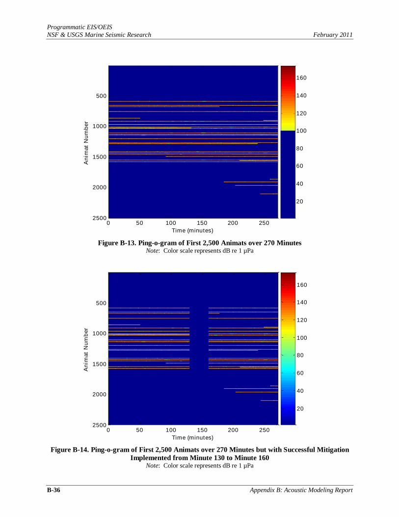
Programmatic EIS/OEIS
NSF & USGS Marine Seismic Research February 2011
B-36 Appendix B: Acoustic Modeling Report
Time (minutes)
An
imat
Nu
mb
er
0 50 100 150 200 250
500
1000
1500
2000
2500
20
40
60
80
100
120
140
160
Figure B-13. Ping-o-gram of First 2,500 Animats over 270 Minutes
Note: Color scale represents dB re 1 µPa
Time (minutes)
An
imat
Nu
mb
er
0 50 100 150 200 250
500
1000
1500
2000
2500
20
40
60
80
100
120
140
160
Figure B-14. Ping-o-gram of First 2,500 Animats over 270 Minutes but with Successful Mitigation
Implemented from Minute 130 to Minute 160 Note: Color scale represents dB re 1 µPa

Programmatic EIS/OEIS
NSF & USGS Marine Seismic Research February 2011
Appendix B:Acoustic Modeling Report B-37
The simulations were created assuming around-the-clock seismic exploration activity. However,
the simulated mitigation was applied only during daylight hours when continuous and at least partially effective visual monitoring would be conducted during seismic operations. Daylight was considered to be
12 hr a day. Based on prior experience, it was assumed that any nighttime visual monitoring that might be
conducted, with or without night vision devices, would have a low probability of detecting marine
mammals. Also, the passive acoustic monitoring (PAM) system, as deployed on the R/V Maurice Ewing in the past and planned for use during some future NSF operations, does not (currently) have sufficient
capabilities to function as an effective mitigation tool. Thus, for the purposes of AIM, no effective
detection-dependent mitigation was assumed to occur during darkness.
7.6 Numbers of Mammals Exposed
Once the effect of mitigation had been considered, the modified exposure history of each animat was analyzed using both pressure and energy units. The JASCO-provided SEL RLs for each airgun shot were converted to rms values by adding 10 dB (i.e., rms = SEL + 10) (see Section 5.2.1).
The maximum rms RL for each animat was then determined, and these values were used to predict the number of modeled ―takes‖ or ―exposures‖ using the traditional NMFS-endorsed exposure
criteria (i.e., rms pressure levels). Level A exposure estimates for cetaceans were those that exceeded 180 dB re 1 µPa (rms) while Level B exposures were those that exceeded 160 dB re 1 µPa (rms). The criteria
used for pinnipeds and fissipeds (sea otter) were 190 and 160 dB re 1 µPa (rms) for Level A and B,
respectively. Note that the exposure numbers at this step are based upon the modeled density of the animats; these numbers are scaled later to represent real-world animal densities.
In addition to these maximum pressure-based exposure estimates, an energy-based metric was calculated. The acoustic exposures that occurred during the 12 hr preceding and following the maximum sound exposure were integrated to produce the energy-based exposure metric for each animat. The
exposure thresholds for this energy-based metric were 198 dB re 1 Pa2 · s SEL for all three groups of
cetaceans and 186 dB re 1 Pa2 · s SEL for pinnipeds in water (LGL 2006). These were calculated for
flat-weighted (unweighted) RLs as well as the M-weighted RLs.
It should be noted that the maximum value of both metrics was calculated for each animat. Therefore each animat in the model can be considered to be taken only once. It is possible that over the
course of a simulation an animal might exceed the thresholds more than once. However, an informal examination of the distribution of exposures for individual animats rarely found a ‗secondary‘ peak of
exposures within the duration of the simulation that would suggest a second threshold exceedance.
The final step was to scale the number of modeled exposures by the ratio of modeling density to real animal density. Individual species density estimates were used for shallow water depths (< 1,000 m)
and deep water (> 1,000 m). To illustrate, consider an example of one simulation that had 20 exposures
above a threshold, 10 of which occurred in shallow water and 10 in adjacent deep water. In this example,
the over-populated modeling density of 4,000 animats resulted in an overall average density of 0.1 animats/square km (km
2), whereas the shallow water density of real word animals is 0.025 animals/ km
2,
and the adjacent deep water density is 0.01 animals/ km2 (Table B-7). This diversity by regional animal
density is accommodated in developing actual, real world exposure estimates. Thus, the number of predicted exposures in each area is different, reflecting the differences in animal abundance.
Table B-7. Nominal Example of Exposure Calculation
Area
Modeled
Exposures
Model
Density
Real World
Density
Real World
Exposures
Shallow Water 10 0.1 0.025 2.5
Deep Water 10 0.1 0.01 1.0

Programmatic EIS/OEIS
NSF & USGS Marine Seismic Research February 2011
B-38 Appendix B: Acoustic Modeling Report
7.7 Marine Mammal Density Values
7.7.1 S California
The target date for the nominal S California cruise was identified as late spring to early summer.
Therefore real world marine mammal density data for the May–July period were obtained from Table A-1 in Koski et al. (1998) for use in the exposure estimates in this report. Since there are several strata listed
within this table, data for strata 2, 3, 4, and 6 (which include the Santa Barbara Channel and surrounding
waters with similar water depths) were combined for the purposes of this analysis.
7.7.2 Caribbean
Marine mammal density values were taken from Tables 4.11 and 4.12 in Smultea et al. (2004). These tables present density calculations based on sighting data from non-seismic conditions in waters
100 to 1,000 m deep and >1,000 m deep collected in the same region during spring 2004. Unidentified animals have been assigned among species that are expected to occur there based on a literature review
(i.e., including some species that were not sighted during the surveys of Smultea et al. [2004]). The basis
for assigning unidentified species was Table 4.12 in Smultea et al. (2004). Note that these tables originally reported their values as animals/1,000 km
2. These values have been scaled to conform to AIM‘s
use of densities in animals/km2 by dividing the originally reported densities by 1,000.
7.7.3 Galapagos Ridge
Marine mammal density values were taken from Table 4 in Lamont-Doherty Earth Observatory (L-DEO) and NSF (2003). This table was produced from data in Ferguson and Barlow (2001) and the
appendix to that report. The values from Block 142 in Ferguson and Barlow (2001) and adjacent blocks
were used to compute the mean densities that appear in Table 4 of L-DEO and NSF (2003).
7.7.4 W Gulf of Alaska
Cetacean density values were taken directly from Table 8 in L-DEO and NSF (2004)
supplemented with densities for killer whales from strata 9 and 10 in Zerbini et al. (2006). The density value for pinnipeds are based on the densities recorded by Brueggeman et al. (1987 , 1988) adjusted for
changes in population size as described in L-DEO and NSF (2004).
7.7.5 NW Atlantic
The densities used for the NW Atlantic site were the average of the Shelf W and Shelf C strata in Palka (2006). These data were collected during ship surveys in 1998 and aerial surveys in 2004.

Programmatic EIS/OEIS
NSF & USGS Marine Seismic Research February 2011
Appendix B:Acoustic Modeling Report B-39
8 Results
8.1 Sound Propagation Modeling – MONM
The MONM propagation model was run in the full n 2-D sense as described in Section 5.2 for
third-octave frequency bands between 10 and 2,000 Hz. Because the airgun arrays are predominantly low-
frequency sources (see Section 5.1.1), this frequency range is sufficient to capture essentially all of the energy output by the arrays. Geographically rendered maps of the received sound levels in dB re µPa
2 · s
are shown in Annex 5 for each of the modeled source locations, along with range-depth plots for selected
sites. The tables of Annex 6 and in the following sub-sections summarize the results of the acoustic
modeling in terms of radii to threshold values of 170 dB and 180 dB SEL re 1 Pa2 · s (approx. 180 dB
and 190 dB re 1 Pa [rms]). Radii are shown both for unweighted (flat-weighted) RLs and for various M-weightings, as described in Sections 5.2.2 and 7.4. Note that the radial resolution of the model runs was 10 m for the ranges involved in calculation of these radii.
The acoustic level values in the model output represent the SEL metric, a suitable measure of the impact of an impulsive sound because it reflects the total acoustic energy delivered over the duration of
the event at a receiver location. In order to determine the rms SPLs required in defining safety radii and exposure estimates, a pulse duration of 0.1 s was assumed, resulting in a conversion factor of +10 dB.
Thus, rms levels (in dB re 1 Pa) were taken to be 10 dB higher than SEL values in dB re 1 Pa2 · s.
For each sound level threshold, two different statistical estimates of the safety radii are provided in the tables in Annex 6 the 95% radius and the maximum endfire radius. Given a regularly gridded
spatial distribution of modeled RLs, the 95% radius is defined as the radius of a circle that encompasses 95% of the grid points whose value is equal to or greater than the threshold value. This definition is
meaningful in terms of potential impact to an animal because, regardless of the geometrical shape of the
noise footprint for a given threshold level, it always provides a range beyond which no more than 5% of a uniformly distributed population would be exposed to sound at or above that level. The maximum endfire
radius is the radius of a 60 degree angular sector, centered on the along-track axis of the array, that
encompasses all grid points whose value is equal to or greater than the threshold value. The greater of the two metrics for each of the modeling cases is shown in the tables of sections 8.1.1 to 8.1.5. Modeled
sound levels were sampled at several depths at each site, up to the lesser of 2,000 m or the seafloor depth.
This was done on the assumption that, at sites deeper than 2,000 m, marine mammals would not dive
deeply enough to be exposed to sounds at greater depths. The tables list radii based on maximum RLs over these ranges of depths. In all cases, however, the maximum radii actually occurred within the upper
500 m of the water column.
Comparison of measured and modeled sound level values in the past has indicated that a precautionary adjustment of 3 dB should be added to the MONM results in some shallow water situations,
particularly where the bottom type is not well known (MacGillivray and Hannay 2007). This will
minimize the likelihood of encountering situations where measured values will exceed predicted values. As such, model predictions for the shallow and slope sites are shown both with and without this
adjustment in the tables of Annex 6:. In this and the following sections, the corrected model predictions
are typically presented, unless otherwise indicated.
The number of predicted exposures in each area is different, reflecting the differences in animal abundance. Note that this separation was done for pressure-based exposure estimates because they are
based upon a single sound exposure that can easily be located within these depth bins. The energy-based
exposure metric is calculated over a 24-hr period, and it is possible that an animal could move back and forth between the shallow and deep water areas during the 24-hr period. Therefore, energy-based
exposure estimates were not stratified by water depth, and the higher of the two animal density numbers
were used to scale from modeled to real world exposure numbers.

Programmatic EIS/OEIS
NSF & USGS Marine Seismic Research February 2011
B-40 Appendix B: Acoustic Modeling Report
8.1.1 S California
Table B-8. Summary of Predicted Marine Mammal Exposure Criteria Radii for the S California
Sites Water Depth Radius (m)*
Site (m) M-weighting 180 dB rms 190 dB rms
Unweighted 45 20
LF cetaceans 50 20
1 100-1,000 MF cetaceans 30 10
HF cetaceans 30 10
Pinnipeds 40 10
Unweighted 64 14
LF cetaceans 64 14
2 100-1,000 MF cetaceans 28 <10
HF cetaceans 22 <10
Pinnipeds 42 14 Notes: *Radii shown are the more conservative (larger) of the values for each site in the tables of Annex 6, and
represent a maximum over all modeled depths, up to the lesser of 2,000 m or seafloor depth, with a 3-dB precautionary factor added to the raw model output for sites with a water depth less than 1,000 m. Source is
a pair of 45/105 in3 GI guns, at a depth of 2.5 m.
8.1.2 Caribbean
Table B-9. Summary of Predicted Marine Mammal Exposure Criteria Radii for the Caribbean
Sites Water Depth Radius (m)*
Site (m) M-weighting 180 dB rms 190 dB rms
Unweighted 1,379 380
LF cetaceans 1,338 366
1 <100 MF cetaceans 533 117
HF cetaceans 447 81
Pinnipeds 815 262
Unweighted 806 252
LF cetaceans 741 226 2 >1,000 MF cetaceans 232 71
HF cetaceans 182 61
Pinnipeds 326 102
Unweighted 524 272
LF cetaceans 508 260
3 100-1,000 MF cetaceans 342 104
HF cetaceans 257 82
Pinnipeds 446 149
Unweighted 802 247
LF cetaceans 738 229
4 >1,000 MF cetaceans 234 72
HF cetaceans 180 58
Pinnipeds 326 102 Notes: *Radii shown are the more conservative (larger) of the values for each site in the tables of Annex 6 and
represent a maximum over all modeled depths, up to the lesser of 2,000 m or seafloor depth, with a 3 dB precautionary factor added to the raw model output for sites with a water depth less than 1,000 m. Source is a 36-gun array (6,600 in3), at a depth of 12 m.

Programmatic EIS/OEIS
NSF & USGS Marine Seismic Research February 2011
Appendix B:Acoustic Modeling Report B-41
8.1.3 Galapagos Ridge
Table B-10. Summary of Predicted Marine Mammal Exposure Criteria Radii for the Galapagos
Ridge Sites Water depth Radius (m)*
Site (m) M-weighting 180 dB rms 190 dB rms
Unweighted 360 110
LF cetaceans 345 110
1-0° >1,000 MF cetaceans 180 60
HF cetaceans 140 50
Pinnipeds 260 81
Unweighted 357 110
LF cetaceans 345 110
1-90° >1,000 MF cetaceans 180 60
HF cetaceans 140 50
Pinnipeds 260 81 Notes: *Radii shown are the more conservative (larger) of the values for each site in the tables of Annex 6, and
represent a maximum over all modeled depths, up to the lesser of 2,000 m or seafloor depth, with a 3 dB precautionary factor added to the raw model output for sites with a water depth less than 1,000 m. Source is an 18-gun array (3,300 in3), at a depth of 6 m.
8.1.4 W Gulf of Alaska
Table B-11. Summary of Predicted Marine Mammal Exposure Criteria Radii for the W Gulf of
Alaska Sites Water Depth Radius (m)*
Site (m) M-weighting 180 dB rms 190 dB rms
Unweighted 1,012 206
LF cetaceans 1,012 209
1 <100 MF cetaceans 478 139
HF cetaceans 398 63
Pinnipeds 885 196
Unweighted 595 155
LF cetaceans 541 152
2 100-1,000 MF cetaceans 262 76
HF cetaceans 202 63
Pinnipeds 390 114
Unweighted 347 104
LF cetaceans 342 103 3 >1,000 MF cetaceans 177 54
HF cetaceans 139 45
Pinnipeds 264 76 Notes: *Radii shown are the more conservative (larger) of the values for each site in the tables of Annex 6, and represent a
maximum over all modeled depths, up to the lesser of 2,000 m or seafloor depth, with a 3 dB precautionary factor added to the raw model output for sites with a water depth less than 1,000 m. Source is an 18-gun array (3,300 in3),
at a depth of 6 m.

Programmatic EIS/OEIS
NSF & USGS Marine Seismic Research February 2011
B-42 Appendix B: Acoustic Modeling Report
8.1.5 NW Atlantic
Table B-12. Summary of Predicted Marine Mammal Exposure Criteria Radii for the NW Atlantic
Sites Water Depth Radius (m)*
Site (m) M-weighting 180 dB rms 190 dB rms
Unweighted 64 14
LF cetaceans 64 14
1 <100 MF cetaceans 28 <10
HF cetaceans 28 <10
Pinnipeds 42 14
Unweighted 57 14
LF cetaceans 57 14
2 100-1,000 MF cetaceans 28 <10
HF cetaceans 28 <10
Pinnipeds 42 14
Unweighted 36 14 LF cetaceans 36 14
3 >1,000 MF cetaceans 14 <10
HF cetaceans 14 <10
Pinnipeds 28 <10
Unweighted 57 14
LF cetaceans 57 14
4 100-1,000 MF cetaceans 28 <10
HF cetaceans 22 <10
Pinnipeds 42 14 Notes: *Radii shown are the more conservative (larger) of the values for each site in the Annex 6 tables. They represent a
maximum over all modeled depths, up to the lesser of 2,000 m or seafloor depth, with a 3-dB precautionary factor added to the raw model output for sites with a water depth < 1,000 m. Source is a pair of 45/105 in3 GI guns, 2.5 m depth.
8.2 SELs and 90% RMS SPLs
The acoustic levels predicted by the model output are expressed as SEL values. SEL is a suitable measure of the potential impact of an impulsive noise because it reflects the total acoustic energy
delivered over the duration of the event at a receiver location. An impact threshold based on the SEL
metric provides a consistent and readily applicable criterion useful with either measured or modeled noise levels. The Noise Criteria Group has concluded that, under most conditions, an energy-based metric such
as SEL would be a better predictor of auditory injury than is pressure (Southall et al. 2007). For this
reason, this analysis (see Section 8.4, below) concentrates on predicting the numbers of marine mammals that might be exposed to various received energy levels. The Noise Criteria Group also recommends a
―do not exceed‖ peak pressure criterion, but under field conditions the SEL criterion is the one that would
be exceeded first and thus would be the operative criterion (Southall et al. 2007).
However, regulatory practice in the U.S., insofar as impulsive underwater sounds are concerned, has to date been based on rms sound pressure level. Thus, there is also interest in predicting the rms RLs
of airgun pulses. As discussed in Section 5.2.1, while existing safety radii regulations in the U.S. are
based on the 90% rms SPL metric for impulsive noise sources, the sensitivity of rms levels to the specific multipath arrival patterns involved is such that model predictions of rms levels at any significant distance
from the source are less accurate than are predicted SEL values. As such, the MONM algorithm does not
attempt to directly model the rms level, but instead models the propagation of acoustic energy in 1/3-
octave bands in a realistic, range-dependent acoustic environment. The rms values may then be estimated
from predicted SEL values based on heuristic estimates of the pulse length. However, the rms estimates
are less reliable than the SEL estimates, as the relationship between the two can vary considerably with

Programmatic EIS/OEIS
NSF & USGS Marine Seismic Research February 2011
Appendix B:Acoustic Modeling Report B-43
range and propagation conditions. Site-specific field measurements would be necessary to resolve this
uncertainty.
8.3 Comparison with Free-field Models
Seismic industry estimates of the sound fields around airgun arrays are typically based on ―free-field‖ sound level calculations that assume uniform sound spreading in an infinite, homogenous ocean.
These free-field estimates neglect specific environmental effects, such as water column refraction and bottom reflections, both of which are taken into account in MONM. In interpreting the results from this
modeling study against sound level and safety range predictions provided by free-field models used in
designing and optimizing airgun arrays, it must always be kept in mind that there are fundamental differences between these modeling approaches that strongly affect the conditions of their applicability.
Specifically, as discussed in the subsections below, free-field models are valid only in the near field, in
close proximity to the source, whereas the MONM is valid in the far field and only for shallow propagation angles (Figure B-15). These differences in how MONM and free-field estimates are obtained
and the regions in which they are appropriate must be taken into account when comparing the sound level
predictions provided by the current study to free-field estimates.
Figure B-15. Stylized Diagram Showing Approximate Regions of Applicability of the MONM and
Free-field Models
8.3.1 TL Estimates
In deep water and for a source close to the sea surface (Figure B-15), acoustic TL may be described by the ―Lloyd-mirror‖ effect — the interference of a sound source with its surface reflection or
―ghost‖ — and simple free-field spherical spreading. An advantage of the free-field Lloyd-mirror model is its simplicity: acoustic TL is modeled by spherical spreading with a simple phase delay for the ghost.
However, the Lloyd-mirror description is only valid at very short ranges from the source (less than a
single water depth) where bottom reflections and water column refraction are unimportant.
In order to accurately predict received sound levels at longer ranges one must take into account reflection and absorption of sound by the sea-bottom and sound refraction in the water column. MONM
satisfies this requirement by applying a variant of the numerical acoustic TL model RAM (based on the
parabolic equation solution to the wave equation) to accurately account for these effects in a realistic environment. This increase in accuracy, however, comes at a significant computational cost and so two
simplifications are necessary to make the hundreds of kilometers of TL computations feasible:
MONM models sound transmission for an equivalent point-like acoustic source combined with
an azimuthal directivity function, and
MONM models transmission of acoustic energy in 1/3-octave bands.
Approximating the airgun array as an omnidirectional source results in under-estimation of RLs directly underneath the array (for the reasons outlined in Section 4.2), where free-field models produce

Programmatic EIS/OEIS
NSF & USGS Marine Seismic Research February 2011
B-44 Appendix B: Acoustic Modeling Report
more accurate results. However, beyond a very short range, the vertically projected component of the
array‘s acoustic energy contributes negligibly to the RL at shallow propagation angles. Thus, MONM is able to predict TL as longer ranges, where the free-field model is not applicable. As discussed in Section
5.2, although the 1/3-octave band approach cannot be used to replicate the acoustic signal in the time-
domain, it is widely used in the acoustics community to characterize the energy of the sound field produced by broadband sources.
As long as environmental conditions are well defined, RAM provides physically accurate predictions of transmission loss for long-range propagation. This is borne out by numerical comparisons of RAM with benchmark acoustic propagation models (Collins et al. 1996; Hannay and Racca 2005).
8.3.2 Near-field vs. Far-field Estimates
An airgun array consists of multiple sources and therefore the first simplification above is not
valid in the near field, close to the array. In the far field, on the other hand, an array radiates as a single acoustic source whose SL is dependent only on the propagation angle (both horizontal and vertical) from
the array (see also Sections 4.2 and 5.1). The acoustic model RAM only computes acoustic transmission
from a point-like, non-directional acoustic source; therefore, for each propagation bearing, MONM uses a different SL based on the horizontal directivity pattern of the airgun array to compute the RL. This
approximation is valid for propagation at shallow vertical angles, but is not applicable in the region
immediately above and below the array as shown in Figure B-15, as discussed above. Conversely, while the Lloyd-mirror approximation is only valid close to the array, in that region it does properly account for
near-field interference effects between array elements.
Note that if we were to neglect the propagation modeling component of MONM, the source
modeling component alone produces results that are consistent with free-field models.
8.4 Marine Mammal Exposure Modeling – AIM
Table B-4 shows the predicted mitigation radii under Alternative A and Alternative B (Preferred
Alternative) for shallow and deep portions of each modeled DAA. For each of the five DAAs, two examples are provided of the modeled population exposure distributions. These graphs show the numbers
of animats predicted to be exposed to various rms levels. These distributions are shown separately for the
shallow and deep portions of each modeling area. Only the portions of these distributions above 155 dB
re 1 µPa (rms) are shown, to provide greater detail in the portion of the distribution that includes the RLs that lead to Level A and Level B exposures. If the entire distribution was presented, the much larger
number of lower RLs would obscure the relevant portion of the distribution (e.g., above 155 dB). It
should be noted that the numbers of exposures in the figures are for the modeled population.
In addition, for the tables of predicted exposures in both SPL and SEL levels, JASCO provided transmission loss in units of M-weighted SEL that were normalized to a 1-second duration. These were
converted to dB rms for the pressure exposure results. Under this methodology, the maximum value for each animat was selected to represent the exposure of that animat. This value was then compared against
the appropriate thresholds to determine if each individual exposure would be considered a ―pressure
take‖.
The procedure to estimate the energy-based exposure began with determining the maximum pressure level, as above. Once the time of that maximum pressure exposure was determined, all exposures
that occurred 12 hours prior to, and following, the maximum exposure were selected. These were
converted from decibels to a linear pressure squared metric. All of the measures from the 24-hour period were then summed and converted back to a decibel metric.
The difference in the values in the pressure and energy take tables is largely due to the differences
in the threshold values. To illustrate, the pressure threshold for mysticete cetaceans was 180 db re 1 Pa
(rms), whereas the energy threshold was 198 dB re 1Pa2 ∙ sec. Therefore a single 181 dB re 1Pa

Programmatic EIS/OEIS
NSF & USGS Marine Seismic Research February 2011
Appendix B:Acoustic Modeling Report B-45
exposure would qualify as a pressure-based take. At the same RL, the animal would need to experience
63 exposures to accumulate sufficient energy to qualify as an energy-based take.
To estimate the actual numbers of marine mammals that would be exposed to sounds at specified levels, the AIM model results for each of the five DAAs were then scaled by the ratio of animat densities
in the model to the real world animal densities. These real-world exposure estimates are provided in table
form for Alternatives A and B.

Programmatic EIS/OEIS
NSF & USGS Marine Seismic Research February 2011
B-46 Appendix B: Acoustic Modeling Report
8.4.1 S California
Figure B-16. Distribution of Modeled Sound Exposures for Common Dolphin in the S California
Site Notes: Only the predicted shallow-water sound exposure distributions are shown for Alternatives A and B, since there was no deep water for this modeling location. See Table B-13 for predicted numbers of real-world exposures.

Programmatic EIS/OEIS
NSF & USGS Marine Seismic Research February 2011
Appendix B:Acoustic Modeling Report B-47
Figure B-17. Distribution of Modeled Sound Exposures for California Sea Lion in the S California
Site Notes: Only the predicted shallow-water sound exposure distributions are shown for Alternatives A and B, since there was no deep water for this modeling location. See Table B-13 for predicted numbers of real-world exposures.

Programmatic EIS/OEIS
NSF & USGS Marine Seismic Research February 2011
B-48 Appendix B: Acoustic Modeling Report
Table B-13. Real World Exposure Predictions for S California Site under Alternatives A and B
Real World Resident Pressure Exposures (Shallow)
Real World Resident Pressure Exposures (Deep)
Real World Energy Exposures
M-weighted Unweighted M-weighted Unweighted M-weighted and Unweighted
Species Level A Level B Level A Level B Level A Level B Level A Level B Level A
Odontocetes
Gervais‘ beaked whale 0.0 0.0 0.0 0.0 0.0 0.0 0.0 0.0 0.0
Blainville‘s beaked whale 0.0 0.0 0.0 0.0 0.0 0.0 0.0 0.0 0.0
Rough-toothed dolphin 0.0 0.0 0.0 0.0 0.0 0.0 0.0 0.0 0.0
Bottlenose dolphin 0.0 0.0 0.0 0.0 0.0 0.0 0.0 0.0 0.0
Pantropical spotted dolphin 0.0 0.0 0.0 0.0 0.0 0.0 0.0 0.0 0.0
Spinner dolphin 0.0 0.0 0.0 0.0 0.0 0.0 0.0 0.0 0.0
Clymene dolphin 0.0 0.0 0.0 0.0 0.0 0.0 0.0 0.0 0.0
Striped dolphin 0.0 0.0 0.0 0.0 0.0 0.0 0.0 0.0 0.0
Common dolphin 0.0 270.4 0.0 1,802.6 0.0 0.0 0.0 0.0 0.0
False killer whale 0.0 0.0 0.0 0.0 0.0 0.0 0.0 0.0 0.0
Short-finned pilot whale 0.0 0.0 0.0 0.0 0.0 0.0 0.0 0.0 0.0
Northern right whale dolphin 0.0 0.0 0.2 4.7 0.0 0.0 0.0 0.0 0.0
Harbor porpoise 0.0 0.0 0.0 0.0 0.0 0.0 0.0 0.0 0.0
Dall's porpoise 0.0 13.5 3.4 45.7 0.0 0.0 0.0 0.0 0.0
Pacific white-sided dolphin 3.2 12.9 3.2 71.0 0.0 0.0 0.0 0.0 0.0
Killer whale 0.0 0.2 0.0 1.0 0.0 0.0 0.0 0.0 0.0
Kogia spp. 0.0 0.0 0.0 0.0 0.0 0.0 0.0 0.0 0.0
Mysticetes
Humpback whale 0.0 0.0 0.0 0.0 0.0 0.0 0.0 0.0 0.0
Minke whale 0.0 0.5 0.0 0.5 0.0 0.0 0.0 0.0 0.0
Bryde‘s whale 0.0 0.0 0.0 0.0 0.0 0.0 0.0 0.0 0.0
Sei whale 0.0 0.0 0.0 0.0 0.0 0.0 0.0 0.0 0.0
Fin whale 0.0 0.0 0.0 0.0 0.0 0.0 0.0 0.0 0.0
Gray whale 0.0 0.0 0.0 0.0 0.0 0.0 0.0 0.0 0.0
Blue whale 0.0 0.0 0.0 0.0 0.0 0.0 0.0 0.0 0.0
Pinnipeds
Harbor seal 0.0 38.5 0.0 50.3 0.0 0.0 0.0 0.0 0.0
N. elephant seal 0.0 137.1 0.0 185.5 0.0 0.0 0.0 0.0 0.0
California sea lion 0.0 2,371.6 0.0 3,613.9 0.0 0.0 0.0 0.0 0.0
Steller‘s sea lion 0.0 0.0 0.0 0.0 0.0 0.0 0.0 0.0 0.0
Guadalupe fur seal 0.0 0.0 0.0 0.0 0.0 0.0 0.0 0.0 0.0
Northern fur seal 0.0 0.0 0.0 0.0 0.0 0.0 0.0 0.0 0.0

Programmatic EIS/OEIS
NSF & USGS Marine Seismic Research February 2011
Appendix B:Acoustic Modeling Report B-49
8.4.2 Caribbean
Figure B-18. Distribution of Modeled Sound Exposures for Bottlenose Dolphin in the Caribbean
Site Notes: The predicted shallow- and deep-water sound exposure distributions are shown for Alternatives A and B. See Table B-14 for predicted numbers of real-world exposures.
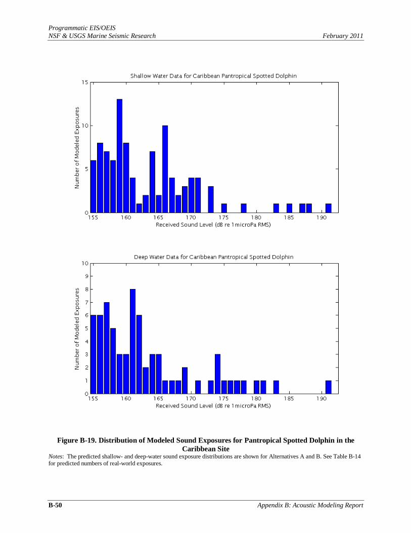
Programmatic EIS/OEIS
NSF & USGS Marine Seismic Research February 2011
B-50 Appendix B: Acoustic Modeling Report
Figure B-19. Distribution of Modeled Sound Exposures for Pantropical Spotted Dolphin in the
Caribbean Site Notes: The predicted shallow- and deep-water sound exposure distributions are shown for Alternatives A and B. See Table B-14 for predicted numbers of real-world exposures.

Programmatic EIS/OEIS
NSF & USGS Marine Seismic Research February 2011
Appendix B:Acoustic Modeling Report B-51
Table B-14. Real World Exposure Predictions for the Caribbean Site under Alternatives A and B
Real World Resident
Pressure Exposures (Shallow)
Real World Resident
Pressure Exposures (Deep)
Real World
Energy Exposures
M-weighted Unweighted M-weighted Unweighted M-weighted Unweighted
Species Level A Level B Level A Level B Level A Level B Level A Level B Level A
Odontocetes
Gervais‘ beaked whale 0.0 0.0 0.0 0.1 0.0 0.0 0.0 0.0 0.0 0.0
Blainville‘s beaked whale 0.0 0.0 0.0 0.1 0.0 0.0 0.0 0.0 0.0 0.0
Rough-toothed dolphin 0.4 8.1 1.7 14.0 0.3 3.0 0.4 12.9 0.0 0.0
Bottlenose dolphin 1.6 43.5 9.8 83.6 0.4 3.6 1.1 10.8 0.0 0.0
Pantropical spotted dolphin 0.7 7.2 1.7 10.5 0.2 2.5 0.4 2.3 0.0 0.1
Atlantic spotted dolphin 10.3 105.3 24.8 152.7 0.7 8.3 1.3 7.8 0.0 2.1
Spinner dolphin 0.1 0.8 0.2 1.2 0.0 0.3 0.0 0.3 0.0 0.0
Clymene dolphin 0.1 0.8 0.2 1.2 0.0 0.3 0.0 0.3 0.0 0.0
Striped dolphin 0.1 0.8 0.2 1.2 1.2 14.9 2.4 14.1 0.0 0.4
Long-beaked common dolphin 2.7 22.4 9.0 55.6 0.3 4.2 0.8 8.1 0.0 0.0
Fraser‘s dolphin 0.0 0.3 0.1 0.7 0.0 0.1 0.1 0.4 0.0 0.0
Risso‘s dolphin 0.0 0.2 0.1 0.7 0.0 0.1 0.0 0.5 0.0 0.0
Melon-headed whale 0.0 0.6 0.1 1.5 0.0 0.0 0.0 0.0 0.0 0.0
Pygmy killer whale 0.0 0.6 0.1 1.5 0.0 0.0 0.0 0.0 0.0 0.0
False killer whale 0.0 0.6 0.1 1.5 0.0 0.0 0.0 0.0 0.0 0.0
Short-finned pilot whale 0.3 6.8 1.7 18.0 0.1 4.0 1.3 10.5 0.0 0.0
Killer whale 0.0 1.0 0.2 2.1 0.0 0.0 0.0 0.0 0.0 0.0
Sperm whale 0.0 0.4 0.2 2.9 0.0 2.0 0.3 14.2 0.0 0.0
Kogia spp. 0.0 0.1 0.0 0.2 0.0 0.0 0.0 0.0 0.0 0.0
Mysticetes
Humpback whale 0.0 0.3 0.0 0.3 0.0 0.0 0.0 0.0 0.004 0.0
Minke whale 0.0 0.0 0.0 0.0 0.0 0.0 0.0 0.0 0.0 0.0
Bryde‘s whale 0.3 1.4 0.3 1.4 0.0 0.0 0.0 0.0 0.019 0.0
Sei whale 0.0 0.0 0.0 0.0 0.0 0.0 0.0 0.0 0.0 0.0
Fin whale 0.0 0.2 0.0 0.2 0.0 0.0 0.0 0.0 0.006 0.0
Blue whale 0.0 0.0 0.0 0.0 0.0 0.0 0.0 0.0 0.0 0.0

Programmatic EIS/OEIS
NSF & USGS Marine Seismic Research February 2011
B-52 Appendix B: Acoustic Modeling Report
8.4.3 Galapagos Ridge
Figure B-20. Distribution of Modeled Sound Exposures for Bryde’s Whale in the Galapagos Ridge
Site Notes: Only the predicted deep-water sound exposure distributions are shown for Alternatives A and B, since there was no shallow water for this modeling location. See Table B-15 for predicted numbers of real-world exposures.

Programmatic EIS/OEIS
NSF & USGS Marine Seismic Research February 2011
Appendix B:Acoustic Modeling Report B-53
Figure B-21. Distribution of Modeled Sound Exposures for Pantropical Spotted Dolphin in the
Galapagos Ridge Site Notes: Only the predicted deep-water sound exposure distributions are shown for Alternatives A and B, since there was no shallow water for this modeling location. See Table B-15 for predicted numbers of real-world exposures.

Programmatic EIS/OEIS
NSF & USGS Marine Seismic Research February 2011
B-54 Appendix B: Acoustic Modeling Report
Table B-15. Real World Exposure Predictions for the Galapagos Ridge Site under Alternatives A and B
Real World Resident Pressure Exposures (Shallow)
Real World Resident Pressure Exposures (Deep)
Real World Energy Exposures
M-weighted Unweighted M-weighted Unweighted M-weighted Unweighted
Species Level A Level B Level A Level B Level A Level B Level A Level B Level A
Odontocetes
Sperm Whale 0.0 0.0 0.0 0.0 0.0 0.4 0.0 5.7 0.025 0.0
Pygmy sperm whale 0.0 0.0 0.0 0.0 0.0 0.0 0.0 0.0 0.0 0.0
Dwarf sperm whale 0.0 0.0 0.0 0.0 0.0 21.8 3.0 145.3 0.0 0.0
Cuvier‘s beaked whale 0.0 0.0 0.0 0.0 0.0 1.5 0.0 36.2 0.0 0.0
Longman‘s beaked whale 0.0 0.0 0.0 0.0 0.0 0.0 0.0 0.0 0.0 0.0
Pygmy beaked whale 0.0 0.0 0.0 0.0 0.0 0.0 0.0 0.0 0.0 0.0
Blainville‘s beaked whale 0.0 0.0 0.0 0.0 0.0 0.0 0.0 0.0 0.0 0.0
Mesoplodon spp. 0.0 0.0 0.0 0.0 0.0 0.7 0.0 17.7 0.0 0.0
Rough-toothed dolphin 0.0 0.0 0.0 0.0 0.0 16.0 0.0 130.9 0.0 0.0
Bottlenose dolphin 0.0 0.0 0.0 0.0 0.2 10.1 1.0 69.5 0.0 0.0
Pantropical spotted dolphin 0.0 0.0 0.0 0.0 9.6 325.7 67.1 2,232.0 0.0 0.0
Spinner dolphin 0.0 0.0 0.0 0.0 4.7 174.0 32.9 1,095.4 0.0 0.0
Costa Rican spinner dolphin 0.0 0.0 0.0 0.0 0.0 0.0 0.0 0.0 0.0 0.0
Clymene dolphin 0.0 0.0 0.0 0.0 0.0 0.0 0.0 0.0 0.0 0.0
Striped dolphin 0.0 0.0 0.0 0.0 4.2 141.5 29.1 969.5 0.0 0.0
Short-beaked common dolphin 0.0 0.0 0.0 0.0 0.1 2.9 0.6 22.5 0.0 0.0
Fraser‘s dolphin 0.0 0.0 0.0 0.0 0.1 2.2 0.6 11.0 0.0 0.0
Risso‘s dolphin 0.0 0.0 0.0 0.0 0.0 7.8 0.7 56.3 0.0 0.0
Melon-headed whale 0.0 0.0 0.0 0.0 0.0 3.3 0.5 25.7 0.0 0.0
Pygmy killer whale 0.0 0.0 0.0 0.0 0.0 5.7 0.8 44.8 0.0 0.0
False killer whale 0.0 0.0 0.0 0.0 0.0 1.7 0.3 13.5 0.0 0.0
Short-finned pilot whale 0.0 0.0 0.0 0.0 0.0 12.9 1.9 100.8 0.0 0.0
Killer whale 0.0 0.0 0.0 0.0 0.0 0.6 0.0 3.0 0.0 0.0
Mysticetes
Humpback whale 0.0 0.0 0.0 0.0 0.0 0.0 0.0 0.0 0.0 0.0
Minke whale 0.0 0.0 0.0 0.0 0.0 0.0 0.0 0.0 0.0 0.0
Bryde‘s whale 0.0 0.0 0.0 0.0 0.6 16.8 0.6 21.1 0.0 0.0
Sei whale 0.0 0.0 0.0 0.0 0.0 0.0 0.0 0.0 0.0 0.0
Fin whale 0.0 0.0 0.0 0.0 0.0 0.0 0.0 0.0 0.0 0.0
Blue whale 0.0 0.0 0.0 0.0 0.0 0.9 0.0 1.1 0.0 0.0

Programmatic EIS/OEIS
NSF & USGS Marine Seismic Research February 2011
Appendix B:Acoustic Modeling Report B-55
8.4.4 W Gulf of Alaska
Figure B-22. Distribution of Modeled Sound Exposures for Fin Whale in the W Gulf of Alaska Site Notes: The predicted shallow- and deep-water sound exposure distributions are shown for Alternatives A and B. See Table B-16 for predicted numbers of real-world exposures.

Programmatic EIS/OEIS
NSF & USGS Marine Seismic Research February 2011
B-56 Appendix B: Acoustic Modeling Report
Figure B-23. Distribution of Modeled Sound Exposures for Steller’s Sea Lion in the W Gulf of
Alaska Site Notes: The predicted shallow- and deep-water sound exposure distributions are shown for Alternatives A and B. See Table B-16 for predicted numbers of real-world exposures.

Programmatic EIS/OEIS
NSF & USGS Marine Seismic Research February 2011
Appendix B:Acoustic Modeling Report B-57
Table B-16. Real World Exposure Predictions for the W Gulf of Alaska Site under Alternatives A and B
Real World Resident Pressure Exposures (Shallow)
Real World Resident Pressure Exposures (Deep)
Real World Energy Exposures
M-weighted Unweighted M-weighted Unweighted M-weighted Unweighted
Species Level A Level B Level A Level B Level A Level B Level A Level B Level A
Odontocetes
Sperm whale 0.0 2.5 0.3 4.8 0.0 0.4 0.0 3.1 0.0 0.0
Cuvier‘s beaked whale 0.4 12.6 1.0 25.8 0.0 1.1 0.1 16.9 0.0 0.1
Baird‘s beaked whale 0.1 3.9 0.3 7.9 0.0 0.3 0.0 5.2 0.0 0.0
Stejneger‘s beaked whale 0.0 0.0 0.0 0.0 0.0 0.0 0.0 0.0 0.0 0.0
Beluga whale 0.0 0.0 0.0 0.0 0.0 0.0 0.0 0.0 0.0 0.0
Pacific white-sided dolphin 0.1 7.3 1.1 14.0 0.1 4.0 0.3 12.3 0.0 0.0
Risso‘s dolphin 0.0 0.0 0.0 0.0 0.0 0.0 0.0 0.0 0.0 0.0
Killer whale 0.2 8.9 1.2 18.6 0.0 3.0 0.8 7.1 0.0 0.0
Short-finned pilot whale 0.0 0.0 0.0 0.0 0.0 0.0 0.0 0.0 0.0 0.0
Harbor porpoise 0.5 61.7 15.1 137.4 0.0 17.9 4.3 27.0 0.0 0.0
Dall's porpoise 9.5 482.2 133.7 1,269.8 0.0 176.6 33.4 377.1 0.0 0.0
Mysticetes
N Pacific right whale 0.0 0.2 0.0 0.2 0.0 0.1 0.0 0.1 0.0 0.0
Gray whale 9.8 115.6 9.3 119.6 2.7 35.1 2.7 32.9 0.0 0.0
Humpback whale 13.6 154.8 14.3 163.7 5.5 31.4 4.8 23.9 0.0 0.0
Minke whale 2.2 36.9 1.9 38.3 0.8 9.5 0.8 7.9 0.0 0.0
Sei whale 0.0 0.0 0.0 0.0 0.0 0.0 0.0 0.0 0.0 0.0
Fin whale 13.7 122.9 12.7 131.4 0.5 39.6 1.1 34.3 0.0 0.0
Blue whale 0.0 0.0 0.0 0.0 0.0 0.0 0.0 0.0 0.0 0.0
Pinnipeds
N fur seal 0.1 9.0 1.3 10.3 0.0 1.0 0.0 1.0 0.1 0.0
California sea lion 0.0 0.0 0.0 0.0 0.0 0.0 0.0 0.0 0.0 0.0
Steller‘s sea lion 0.0 86.3 6.1 109.9 0.9 23.1 0.9 16.1 0.4 0.0
Pacific walrus 0.0 0.0 0.0 0.0 0.0 0.0 0.0 0.0 0.0 0.0
Bearded seal 0.0 0.0 0.0 0.0 0.0 0.0 0.0 0.0 0.0 0.0
Harbor seal 1.4 142.3 13.5 203.2 1.4 32.6 4.2 29.0 1.4 0.0
Spotted seal 0.0 0.0 0.0 0.0 0.0 0.0 0.0 0.0 0.0 0.0
Ringed seal 0.0 0.0 0.0 0.0 0.0 0.0 0.0 0.0 0.0 0.0
Ribbon seal 0.0 0.0 0.0 0.0 0.0 0.0 0.0 0.0 0.0 0.0
N elephant seal 0.0 0.0 0.0 0.0 0.0 0.0 0.0 0.0 0.0 0.0

Programmatic EIS/OEIS
NSF & USGS Marine Seismic Research February 2011
B-58 Appendix B: Acoustic Modeling Report
8.4.5 NW Atlantic
Figure B-24. Distribution of Modeled Sound Exposures for Bottlenose Dolphin in the NW Atlantic
Site Notes: The predicted shallow- and deep-water sound exposure distributions are shown for Alternatives A and B. See Table B-17 for predicted numbers of real-world exposures.

Programmatic EIS/OEIS
NSF & USGS Marine Seismic Research February 2011
Appendix B:Acoustic Modeling Report B-59
Figure B-25. Distribution of Modeled Sound Exposures for Sperm Whale in the NW Atlantic Site Notes: The predicted shallow- and deep-water sound exposure distributions are shown for Alternatives A and B. See Table B-17 for predicted numbers of real-world exposures.

Programmatic EIS/OEIS
NSF & USGS Marine Seismic Research February 2011
B-60 Appendix B: Acoustic Modeling Report
Table B-17. Real World Exposure Predictions for the NW Atlantic Site under Alternatives A and B
Real World Resident
Pressure Exposures (Shallow)
Real World Resident
Pressure Exposures (Deep)
Real World
Energy Exposures
M-weighted Unweighted M-weighted Unweighted M-weighted and Unweighted
Species Level A Level B Level A Level B Level A Level B Level A Level B Level A
Odontocetes
Sperm whale 0.3 13.3 0.3 37.9 0.0 0.7 0.3 1.0 0.0
Kogia spp. 0.1 7.8 0.1 20.0 0.0 0.1 0.0 0.3 0.0
Bottlenose whale 0.0 0.0 0.0 0.0 0.0 0.0 0.0 0.0 0.0
Unidentified beaked whale 0.0 3.1 0.0 9.1 0.0 0.0 0.0 0.0 0.0
Bottlenose dolphin 2.1 134.9 2.1 341.6 0.0 2.1 0.0 4.2 0.0
Spotted dolphin 0.0 50.6 0.9 117.0 0.0 0.9 0.0 0.9 0.0
Spinner dolphin 0.0 0.0 0.0 0.0 0.0 0.0 0.0 0.0 0.0
Striped dolphin 0.0 251.9 4.3 581.9 0.0 4.3 0.0 4.3 0.0
Common dolphin 8.0 378.3 8.0 1,118.7 0.0 24.1 0.0 32.2 0.0
Whitesided dolphin 0.0 0.0 0.0 0.0 0.0 0.0 0.0 0.0 0.0
Harbor porpoise 0.0 0.0 0.0 0.0 0.0 0.0 0.0 0.0 0.0
Pilot whale 0.0 0.0 0.0 0.0 0.0 0.0 0.0 0.0 0.0
Mysticetes 0.0
Right whale 0.0 0.2 0.0 0.2 0.0 0.0 0.0 0.0 0.0
Humpback whale 0.0 0.7 0.0 0.7 0.0 0.0 0.0 0.0 0.0
Minke whale 0.0 0.1 0.0 0.1 0.0 0.0 0.0 0.0 0.0
Sei whale 0.0 0.1 0.0 0.1 0.0 0.0 0.0 0.0 0.0
Fin whale 0.0 1.3 0.0 1.3 0.0 0.0 0.0 0.0 0.0

Programmatic EIS/OEIS
NSF & USGS Marine Seismic Research February 2011
Appendix B:Acoustic Modeling Report B-61
9 Literature Cited
Austin, M.E., A.O. MacGillivray, D.E. Hannay, and S.A. Carr. 2003. Acoustic Monitoring of Marathon Canada Petroleum ULC 2003 Courland/Empire Seismic Program. Marathon Canada Petroleum ULC, by JASCO Research Ltd.
Barlow, J. 1999. Trackline detection probability for long-diving whales. Pages 209-221 in G.W. Garner, S.C. Amstrup, J.L. Laake, B.F.J. Manly, L.L. McDonald, and D.G. Robertson, eds. Marine Mammal
Survey and Assessment Methods. A.A Balkema, Brookfield, VT.
Barrie, J.V. and B.D. Bornhold. 1989. Surficial geology of Hecate Strait, British Columbia continental shelf. Canadian Journal of Earth Sciences 26:1241-1254.
Becker, K., A. Bartetzko, and E.E. Davis. 2001. Leg 174B synopsis: revisiting Hole 395A for logging and long-term monitoring of off-axis hydrothermal processes in young oceanic crust. In K. Becker
and M.J. Malone, eds. Proceedings of the Ocean Drilling Program, Scientific Results, Volume 174B.
Available from http://www-odp.tamu.edu/publications/174B_SR/synopsis/synopsis.htm.
Bishop, G.C., W.T. Ellison, and L.E. Mellberg. 1987. A simulation model for high-frequency under-ice reverberation. Journal of the Acoustical Society of America 82:275-285.
Blackwell, S.B., R.G. Norman, C.R. Greene Jr. and W.J. Richardson. 2007. Acoustic measurements.
Pages 4-1 – 4-52 in Marine mammal monitoring and mitigation during open water seismic exploration by Shell Offshore Inc. in the Chukchi and Beaufort Seas, July-September 2006: 90-day
report. LGL Report P891-1. Prepared by LGL Alaska Research Associates Inc., Anchorage, AK,
and Greeneridge Sciences Inc., Santa Barbara, CA, for Shell Offshore Inc., Houston, TX, National Marine Fisheries Service, Silver Spring, MD, and U.S. Fish & Wildlife Service, Anchorage, AK.
Brueggeman, J.J., G.A. Green, R.A. Grotefendt, and D.G. Chapman. 1987. Aerial surveys of endangered cetaceans and other marine mammals in the northwestern Gulf of Alaska and southeastern Bering
Sea. Outer Continental Shelf Environmental Assessment Program, Final Report, Principal Investigation 61(1989):1-124. OCS Study MMS 89-0026. Minerals Management Service, Anchorage,
AK.
Brueggeman, J.J., G.A. Green, R.W. Tressler, and D.G. Chapman. 1988. Shipboard surveys of endangered cetaceans in the northwestern Gulf of Alaska. OCS Environmental Assessment Program
Final Report, Principal Investigation 61(1989):125-188. OCS Study MMS 89-0026. Prepared by
Envirosphere Company for Minerals Management Service, Alaska OCS Office and NOAA, Office of Oceanography and Marine Assessment, Alaska Office.
Buogo, S. and G.B. Cannelli. 2002. Implosion of an underwater spark-generated bubble and acoustic energy evaluation using the Rayleigh model. Journal of the Acoustical Society of America 111:2594-
2600.
Carey, W.M., J. Doutt, R.B. Evans, and L.M. Dillma. 1995. Shallow-water sound transmission measurements on the New Jersey continental shelf. IEEE Journal of Oceanic Engineering 20:321-
336.
Clay, C.S. and H. Medwin. 1977. Acoustical Oceanography. John Wiley & Sons, Inc., New York.
Collins, M.D., R.J. Cederberg, D.B. King, and S.A. Chin-Bing. 1996. Comparison of algorithms for solving parabolic wave equations. Journal of the Acoustical Society of America 100:178-182.
Coppens, A.B. 1981. Simple equations for the speed of sound in Neptunian waters. Journal of the Acoustical Society of America 69:862–863.

Programmatic EIS/OEIS
NSF & USGS Marine Seismic Research February 2011
B-62 Appendix B: Acoustic Modeling Report
Divins, D.L. 2006. NGDC Total Sediment Thickness of the World's Oceans & Marginal Seas.
http://www.ngdc.noaa.gov/mgg/sedthick/sedthick.html. Accessed November.
Dragoset, W.H. 1984. A comprehensive method for evaluating the design of airguns and airgun arrays. 16th Annual Proceedings of Offshore Technology Conference 3:75-84.
Edgerton, H.E. and G.G. Hayward. 1964. The ‗Boomer‘ sonar source for seismic profiling. Journal of
Geophysical Research 69:3033-3042.
Einwich, A.E. 1981. Geology related to Acoustic transmission: Eastern Caribbean. Naval Ocean Research and Development Activity, NSTL Station, MS.
Ellison, W.T., R.M. Sonntag, and C.W. Clark. 1987. Comparison of measured bowhead whale, Balaena mysticetus, migration parameters with results from the tracking algorithm. Reports of the
International Whaling Commission 37:309-311.
Ferguson, M.C. and J. Barlow. 2001. Spatial Distributions and Density of Cetaceans in the Eastern Tropical Pacific Ocean Based on Summer/Fall Research Vessel Surveys in 1986-96. National Marine
Fisheries Service, Southwest Fisheries Science Center, La Jolla, CA.
Finneran, J.J., C.E. Schlundt, R. Dear, D.A. Carder, and S.H. Ridgway. 2002. Temporary shift in masked
hearing thresholds in odontocetes after exposure to single underwater impulses from a seismic watergun. Journal of the Acoustical Society of America 111:2929-2940.
Finneran, J.J., D.A. Carder, C.E. Schlundt, and S.H. Ridgway. 2005. Temporary threshold shift in
bottlenose dolphins (Tursiops truncatus) exposed to mid-frequency tones. Journal of the Acoustical Society of America 118:2696-2705.
Francois, R.E. and G.R. Garrison. 1982a. Sound absorption based on ocean measurements. Part I: Pure water and magnesium sulfate contributions. Journal of the Acoustical Society of America 72:896-907.
Francois, R.E. and G.R. Garrison. 1982b. Sound absorption based on ocean measurements. Part II: Boric acid contribution and equation for total absorption. Journal of the Acoustical Society of America
72:1879-1890.
Frankel A.S. and K.V. Vigness-Raposa. 2006. Marine Animal Behavioral Analysis. Marine Acoustics, Inc., Annapolis, MD.
Frankel, A.S., W.T. Ellison, and J. Buchanan. 2002. Application of the Acoustic Integration Model (AIM) to predict and minimize environmental impacts. Pages 1438-1443 in Oceans '02, Vol. 3. Marine Technology Society & IEEE.
Goff, J.A., B.J. Kraft, L.A. Mayer, S.G. Schock, C.K. Sommerfield, H.C. Olson, S.P.S. Gulick, and S. Nordfjord. 2004. Seabed characterization on the New Jersey middle and outer shelf: correlatability
and spatial variability of seafloor sediment properties. Marine Geology 209:147–172.
Goold, J.C. and P.J. Fish. 1998. Broadband spectra of seismic survey air-gun emissions, with reference to dolphin auditory thresholds. Journal of the Acoustical Society of America 103:2177-2184.
Greene, C.R., Jr. and W.J. Richardson. 1988. Characteristics of marine seismic survey sounds in the Beaufort Sea. Journal of the Acoustical Society of America 83:2246-2254.
Greene, C.R., Jr., J.S. Hanna, and R.W. Blaylock. 1997. Physical acoustics measurements. Pages 3-1 – 3-63 in W.J. Richardson, ed. Northstar Marine Mammal Monitoring Program, 1996: Marine Mammal and Acoustical Monitoring of a Seismic Program in the Alaskan Beaufort Sea. LGL Rep. 2121-2.
Prepared by LGL Ltd., King City, ON, and Greeneridge Sciences Inc., Santa Barbara, CA, for BP
Exploration (Alaska) Inc., Anchorage, AK, and NMFS, Anchorage, AK, and Silver Spring, MD.

Programmatic EIS/OEIS
NSF & USGS Marine Seismic Research February 2011
Appendix B:Acoustic Modeling Report B-63
Guerin, G. 2000. Acoustic and Thermal Characterization of Oil Migration, Gas Hydrates Formation and
Silica Diagenesis. Dissertation, Columbia University, NY.
Haley, B. 2006. Marine mammal monitoring during University of Texas at Austin‘s marine geophysical survey of the Western Canada Basin, Chukchi Borderland and Mendeleev Ridge, Arctic Ocean, July–
August 2006. LGL Rep. TA4285-3. Prepared by LGL Alaska Research Associates Inc., Anchorage,
AK, and LGL Ltd., King City, ONT, for University of Texas at Austin Institute for Geophysics, Austin, TX; NMFS, Silver Spring, MD; and USFWS, Anchorage, AK. November.
Hamilton, E.L. 1980. Geoacoustic modeling of the sea floor. Journal of the Acoustical Society of America
68:1313-1340.
Hannay, D.E. and R.G. Racca. 2005. Acoustic model validation. Technical report prepared by JASCO Research Ltd. for Sakhalin Energy Investment Company. 18 February. Available at
http://www.sakhalinenergy.com/en/documents/doc_33_jasco.pdf.
Herzig, P.M., S.E. Humphris, D.J. Miller, and R.A. Zierenberg, Eds. 1998. Proceedings of the Ocean Drilling Program, Scientific Results, Volume 158. College Station, TX.
Holland, C.W. 2003. Seabed reflection measurement uncertainty. Journal of the Acoustical Society of
America 114:1861-1873.
Hutchins, R.W., D.L. McKeown, and L.H. Kind. 1976. A deep-tow high resolution seismic system for continental shelf mapping. Geoscience Canada 3:95-100.
James, N.P., Y. Bone, T.K. Kyser, G.R. Dix, and L.B. Collins. 2004. The importance of changing oceanography in controlling late Quaternary carbonate sedimentation on a high-energy, tropical,
oceanic ramp: north-western Australia. Sedimentology 51:1179-1205.
Kastak, D., R.J. Schusterman, B.L. Southall, and C.J. Reichmuth. 1999. Underwater temporary threshold shift induced by octave-band noise in three species of pinniped. Journal of the Acoustical Society of
America 106:1142-1148.
Keenan, R.E., D.F. McCammon, E. Holmes, and M.S. Moustafa. 2001. Resolution and Accuracy of
Environmental Parameters Required for Precise Acoustic Predictions. N774C Report.
Koski, W.R., J.W. Lawson, D.H. Thomson, and W.J. Richardson. 1998. Marine Mammal Technical Report. Point Mugu Sea Range Environmental Impact Statement/Overseas Environmental Impact
Statement. Prepared by LGL Ltd., environmental research associates, King City, ONT, and Ogden Environmental and Energy Services, Santa Barbara, CA, for Naval Air Warfare Center Weapons
Division, Point Mugu, CA. December.
Landro, M. 1992. Modeling of GI gun signatures. Geophysical Prospecting 40:721-747.
Laws, M., L. Hatton, and M. Haartsen. 1990. Computer modeling of clustered airguns. First Break 8:331–338.
L-DEO and NSF. 2003. Environmental Assessment of a Marine Seismic Survey by the R/V Maurice
Ewing in the Hess Deep Area of the Eastern Tropical Pacific Ocean. Prepared by LGL Ltd., environmental research associates, King City, ONT. LGL Report TA2822-4. 18 March.
L-DEO and NSF. 2004. Environmental Assessment of a Marine Geophysical Survey by the R/V Kilo Moana around the Aleutian Islands, June–July 2005. LGL Report 4089-1. Prepared by LGL, Ltd., environmental research associates, King City, ONT. 20 December.
Lurton, X. 2002. An Introduction to Underwater Acoustics: Principles and Applications. Springer, Chichester, UK.
Programmatic EIS/OEIS
NSF & USGS Marine Seismic Research February 2011
B-64 Appendix B: Acoustic Modeling Report
MacGillivray, A.O. 2000. An Acoustic Modeling Study of Seismic Airgun Noise in Queen Charlotte
Basin. Thesis, University of Victoria, BC.
MacGillivray, A.O. and D. Hannay. 2007. Chapter 3: Summary of noise assessment. Pages 3-1 – 3-21 in Marine mammal monitoring and mitigation during open water seismic exploration by ConocoPhillips
Alaska, Inc. in the Chukchi Sea, July-October 2006. LGL Report P903-2. Prepared by LGL Alaska
Research Associates Inc., Anchorage, AK, and JASCO Research Ltd., Victoria, BC, for ConocoPhillips Alaska Inc., Anchorage, AK, and NMFS, Silver Spring, MD.
Malme, C.I., P.W. Smith, and P.R. Miles. 1986. Characterisation of geophysical acoustic survey sounds.
Prepared by BBN Laboratories Inc., Cambridge, for Battelle Memorial Institute to the Minerals Management Service, Pacific Outer Continental Shelf Region, Los Angeles, CA.
McCammon, D.F. 2000. Capturing Uncertainty: Uncertainty in Propagation Loss Calculations. ONR Uncertainty Workshop.
McCauley, R.D., M.-N. Jenner, C. Jenner, K.A. McCabe, and J. Murdoch. 1998. The response of humpback whales (Megaptera novaeangliae) to offshore seismic survey noise: preliminary results of
observations about a working seismic vessel and experimental exposures. APPEA Journal 38:692-
707.
Medwin, H. 2005. Sounds in the Sea: From Ocean Acoustics to Acoustical Oceanography. Cambridge
University Press, NY.
Morales, F.E. and G. Godoy. 1996. Sediment distribution in El Tablazo bay, Maracaibo system, Venezuela. IEEE 3:1492–1496.
Mosher, D.C. and P.G. Simpkin. 1999. Status and trends of marine high-resolution seismic reflection profiling: data acquisition. Geoscience Canada 26:174-188.
NMFS. 2000. Small takes of marine mammals incidental to specified activities; marine seismic-reflection
data collection in southern California. Federal Register 65:16374-16379.
NMFS. 2005. Endangered Fish and Wildlife; Notice of Intent to Prepare an Environmental Impact
Statement. Federal Register 70:1871-1875.
Palka, D.L. 2006. Summer abundance estimates of cetaceans in US North Atlantic Navy Operating Areas. Northeast Fisheries Science Center Reference Document 06-03. NMFS, Northeast Fisheries Science
Center, Woods Hole, MA.
Parkes, G.E. and L. Hatton. 1986. The Marine Seismic Source. Springer, NY
Pirmez, C., R.D. Flood, J. Baptiste, H. Yin, and P.L. Manley. 1997. Clay content, porosity and velocity of Amazon Fan sediments determined from ODP Leg 155 core and wireline logs. Geophysical Research
Letters 24:317–320.
Prell, W.L., N. Niitsuma, et al. 1989. Proceedings of the Ocean Drilling Program, Volume 117, Initial Reports. Ocean Drilling Program, Texas A&M University, College Station, TX. Available at:
http://www-odp.tamu.edu/publications/117_IR/117ir.htm.
Racca, R.G. and J.A. Scrimger. 1986. Underwater Acoustic Source Characteristics of Air and Water Guns. Contractor report by JASCO Research Ltd., Victoria, BC, for DREP. Contract No. 06SB
97708-5-7055.
Reid, J.A. 2005. Point Coverage SCASMPL: Sediment sample data for the Channel Islands and Santa Barbara Channel Region. U.S. Geological Survey.
Programmatic EIS/OEIS
NSF & USGS Marine Seismic Research February 2011
Appendix B:Acoustic Modeling Report B-65
Richardson, W.J., C.R. Greene Jr., C.I. Malme, and D.H. Thomson. 1995. Marine mammals and noise.
Academic Press, San Diego, CA.
Roberts, R.W. 1976. Bottom sediment granulometric data for the Continental margins of the Bering, Chukchi East Siberian, Laptev, and Beaufort Seas. Special Report #70. University of Washington,
Seattle, WA.
Robinson, E.S. and C.S. Çoruh. 1988. Basic Exploration Geophysics. John Wiley & Sons, Inc., New York.
Shore-based Scientific Party. 1994. Site 893, Proceedings of the Ocean Drilling Project, Initial Reports,
Vol. 146 (Part 2). J.P. Kennett, J.G. Baldauf, et al., eds. Ocean Drilling Program, Texas A&M University, College Station, TX.
Shipboard Scientific Party. 1998. Proceedings of the Ocean Drilling Program, Initial Reports, Vol. 174A. J.A. Austin, Jr., N. Christie-Blick, M.J. Malone, et al., eds. Ocean Drilling Program, Texas A&M University, College Station, TX.
Shipboard Scientific Party. 2003a. Leg 203 Summary, Proceedings of the Ocean Drilling Program, Initial Reports, Vol. 203. J.A. Orcutt, A. Schultz, T.A. Davies, et al., eds. Ocean Drilling Program, Texas
A&M University, College Station, TX.
Shipboard Scientific Party. 2003b. Leg 206 Summary, Proceedings of the Ocean Drilling Program, Initial Reports, Vol. 206. D.S. Wilson, D.A.H. Teagle, G.D. Acton, et al., eds. Ocean Drilling Program,
Texas A&M University, College Station, TX.
Smultea, M.A., M. Holst, W.R. Koski, and S. Stoltz. 2004. Marine mammal monitoring during Lamont-Doherty Earth Observatory's seismic program in the Southeast Caribbean Sea and adjacent Atlantic
Ocean, April-June 2004. LGL Rep. TA2822-26. Prepared by LGL Ltd., King City, ONT, for Lamont-Doherty Earth Observatory, Columbia University, Palisades, NY.
Southall, B.L., A.E. Bowles, W.T. Ellison, J.J. Finneran, R.L. Gentry, C.R. Greene, Jr., D. Kastak, D.R. Ketten, J.H. Miller, P.E. Nachtigall, W.J. Richardson, J.A. Thomas, and P.L. Tyack. 2007. Marine
mammal noise exposure criteria: initial scientific recommendations. Aquatic Mammals 33:411-521.
Teague, W.J., M.J. Carron, and P.J. Hogan. 1990. A comparison between the generalized digital environmental model and Levitus climatologies. Journal of Geophysical Research 95(C5):7167-7183.
Thomas, T.A., W.R. Koski, and W.J. Richardson. 2002. Correction factors to calculate bowhead whale numbers from aerial surveys of the Beaufort Sea. Pages 12-1 – 12-38 in W.J. Richardson and D.H.
Thomson, eds. OCS Study MMS 2002-012. U.S. Minerals Management Service, Anchorage, AK, and
Herndon, VA.
Valent, P.J. and H.J. Lee. 1971. NCEL core data – Santa Barbara Channel area, Report #1. Naval Civil Engineering Laboratory, Port Hueneme, CA.
Zerbini, A.N., A. Andriolo, M.P. Heide-Jørsen, J.L. Pizzorno, Y.G. Maia, G.R. VanBlaricom, D.P.
DeMaster, P.C. Simões-Lopes, S. Moreira, and C. Bethlem. 2006. Satellite-monitored movements of humpback whales Megaptera novaeangliae in the Southwest Atlantic Ocean. Marine Ecology
Progress Series 313:295-304.
Zhang, Z. and C. Tindle. 1995. Improved equivalent fluid approximations for a low shear speed ocean bottom. Journal of the Acoustical Society of America 98:3391-3396.
Ziolkowski, A. 1970. A method for calculating the output pressure waveform from an air gun. Geophysical Journal of the Royal Astronomical Society 21:137–161.

Programmatic EIS/OEIS
NSF & USGS Marine Seismic Research February 2011
B-66 Appendix B: Acoustic Modeling Report
[This page intentionally left blank.]

Programmatic EIS/OEIS
NSF & USGS Marine Seismic Research February 2011
Appendix B:Acoustic Modeling Report B-67
Annex 1: Far-field SL Computation
The 1/3-octave band SLs for each modeling azimuth were computed from the horizontally
propagating far-field signature of the array. The far-field signature, sff(t) is the sum of the notional signatures of the individual guns, si(t), time delayed according to their relative position and the
propagation angle:
n
iiff tsts ),()(
where τi is its time-delay of the ith gun in the angular direction (θ, ). For horizontal sound propagation
0 and the time delay is only a function of the azimuthal angle, θ:
cyx iii sincos
where (xi, yi) is the position of gun i in the plane of the array and c is the speed of sound. A plan view diagram, illustrating the geometry of the far-field summation, is shown in Figure A1-1. It is often more
convenient to perform this calculation in the frequency domain by utilizing the Fourier transform shift
theorem, which states that a time delay of τ corresponds to a phase delay of 2πfτ, so that:
n
iiiff yxc
fjfSfS )sincos(
2exp)(),(
where f is frequency and S(f) denotes the Fourier transform of s(t). The far-field signature is then filtered into ⅓-octave pass-bands to generate frequency dependent SLs:
dff
ffSfSL
hi
loffc
2
),(2),(
where SL(fc, θ) is the SL in a 1
/3-octave band with centre frequency fc, in the azimuthal direction θ. Note that the limits of integration in this equation, flo and fhi, are the lower and upper frequency bounds of the 1/3-octave band. Source levels, computed in this way, are suitable for combining with TL output by a
propagation model to compute received sound levels in the far field.
airgun
(xi, y
i)
= 0
i
Figure A1-1. Plan View Diagram of the Far-field Summation Geometry for an Airgun Array

Programmatic EIS/OEIS
NSF & USGS Marine Seismic Research February 2011
B-68 Appendix B: Acoustic Modeling Report
Airgun Model Optimization
A collection of high-quality airgun signature data, obtained from a DREP technical report by Racca and Scrimger [1986], was used to determine optimal values for four empirical model parameters, α,
β, γ and κ. The airgun data were collected by DREP in Jarvis Inlet aboard the CFAV Endeavor as part of a study of the source characteristics of seismic airguns and water-guns. The dataset contains a collection
of 38 back-propagated source signatures for five different Bolt 600/B airguns. The volumes of the airguns
in the dataset are 5 in3, 10 in
3, 40 in
3, 80 in
3 and 185 in
3 and the firing depths of the airguns range from
0.5 m to 10 m.
Best-fit values for the model parameters were obtained using a simulated annealing global optimization algorithm to fit the airgun model to the experimental source signature data.

Programmatic EIS/OEIS
NSF & USGS Marine Seismic Research February 2011
Appendix B:Acoustic Modeling Report B-69
Annex 2: Airgun Array 1/3-Octave Band SLs
Figure A2-1. Directionality of the Airgun Array Source Levels (dB re μPa2 ∙ s) (R/V Langseth 2-D
Reflection, 2 x 1, 650 in3, 6 m tow depth); also 3-D Reflection, two sub-arrays fired in “flip-flop”
fashion).

Programmatic EIS/OEIS
NSF & USGS Marine Seismic Research February 2011
B-70 Appendix B: Acoustic Modeling Report
Figure A2-2. Directionality of the Airgun Array Source Levels (dB re μPa2 ∙ s) (R/V Langseth 2-D
Reflection, 4 x 1, 650 in3, 6 m tow depth)

Programmatic EIS/OEIS
NSF & USGS Marine Seismic Research February 2011
Appendix B:Acoustic Modeling Report B-71
Figure A2-3. Directionality of the Airgun Array Source Levels (dB re μPa2 ∙ s) (R/V Langseth 2-D
Refraction, 4 x 1, 650 in3, 12 m tow depth)
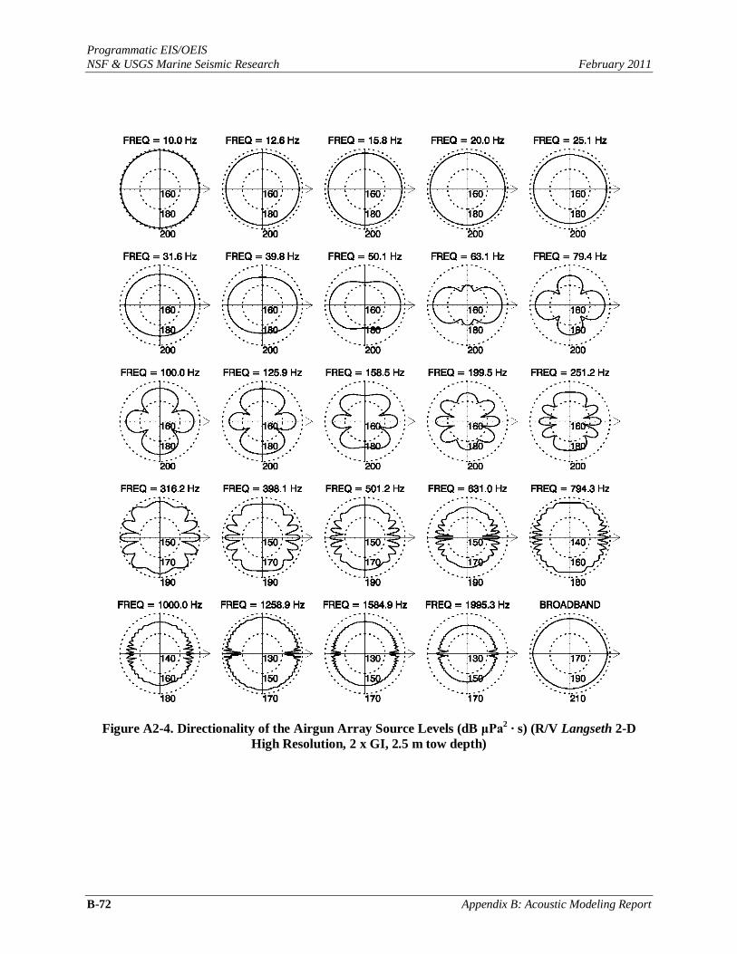
Programmatic EIS/OEIS
NSF & USGS Marine Seismic Research February 2011
B-72 Appendix B: Acoustic Modeling Report
Figure A2-4. Directionality of the Airgun Array Source Levels (dB μPa2 ∙ s) (R/V Langseth 2-D
High Resolution, 2 x GI, 2.5 m tow depth)
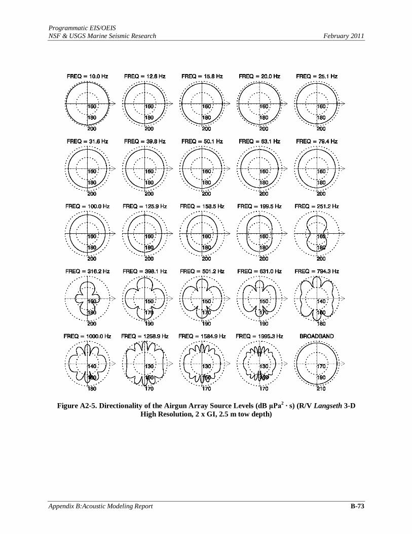
Programmatic EIS/OEIS
NSF & USGS Marine Seismic Research February 2011
Appendix B:Acoustic Modeling Report B-73
Figure A2-5. Directionality of the Airgun Array Source Levels (dB μPa2 ∙ s) (R/V Langseth 3-D
High Resolution, 2 x GI, 2.5 m tow depth)

Programmatic EIS/OEIS
NSF & USGS Marine Seismic Research February 2011
B-74 Appendix B: Acoustic Modeling Report
[This page intentionally left blank.]

Programmatic EIS/OEIS
NSF & USGS Marine Seismic Research February 2011
Appendix B:Acoustic Modeling Report B-75
Annex 3: Source Locations and Study Areas
The locations of modeling sites within each of the five study areas under consideration are shown in Figure A3-1 through Figure A3-5. In each case, the proposed ship‘s track and AIM modeling boundaries are also shown.
Figure A3-1. Locations of S California Modeling Sites

Programmatic EIS/OEIS
NSF & USGS Marine Seismic Research February 2011
B-76 Appendix B: Acoustic Modeling Report
Figure A3-2. Locations of Caribbean Modeling Sites
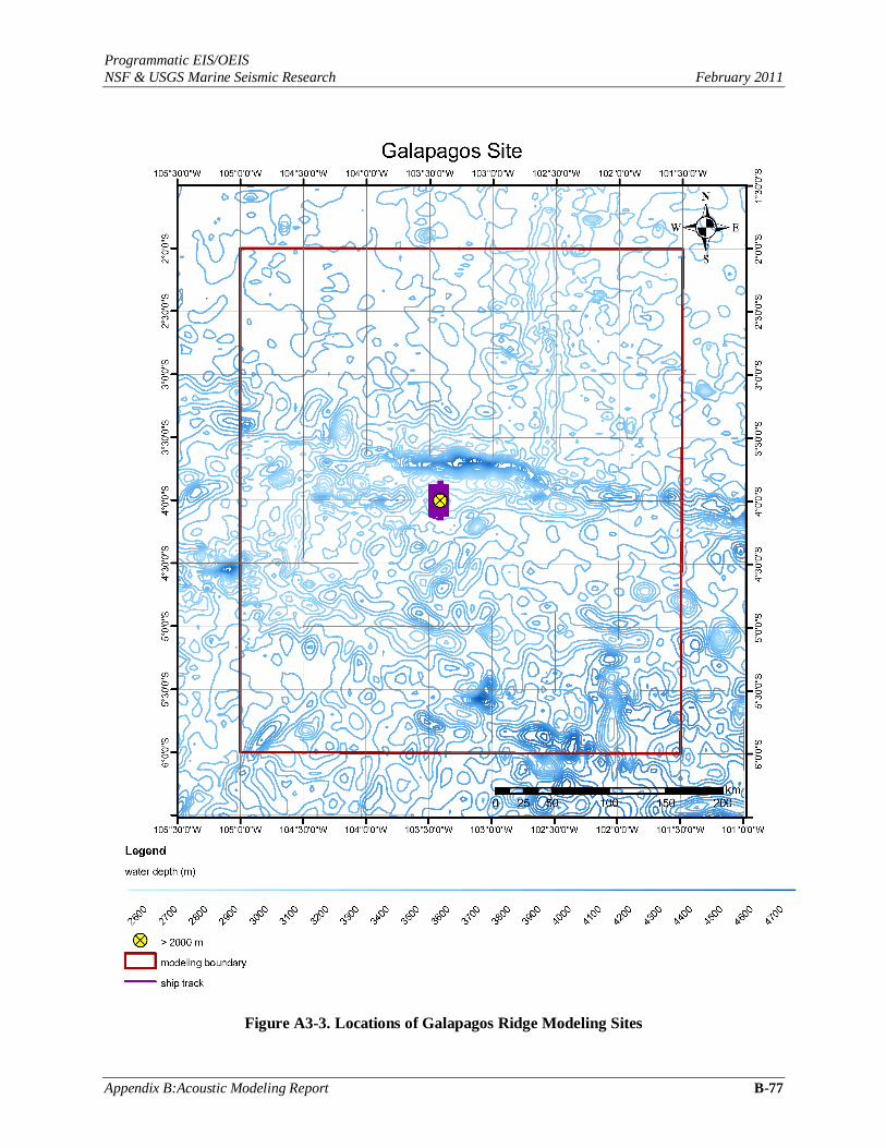
Programmatic EIS/OEIS
NSF & USGS Marine Seismic Research February 2011
Appendix B:Acoustic Modeling Report B-77
Figure A3-3. Locations of Galapagos Ridge Modeling Sites

Programmatic EIS/OEIS
NSF & USGS Marine Seismic Research February 2011
B-78 Appendix B: Acoustic Modeling Report
Figure A3-4. Locations of W Gulf of Alaska Modeling Sites

Programmatic EIS/OEIS
NSF & USGS Marine Seismic Research February 2011
Appendix B:Acoustic Modeling Report B-79
Figure A3-5. Locations of NW Atlantic Modeling Sites

Programmatic EIS/OEIS
NSF & USGS Marine Seismic Research February 2011
B-80 Appendix B: Acoustic Modeling Report
[This page intentionally left blank.]

Programmatic EIS/OEIS
NSF & USGS Marine Seismic Research February 2011
Appendix B:Acoustic Modeling Report B-81
Annex 4: Marine Mammal Species and Associated Densities
and Animat Depth Restrictions Included in AIM
Modeling
This annex includes tables of species modeled for each of the exemplary DAAs. Species that were combined for modeling are highlighted in tan. Refer to Appendix C of the EIS/OEIS for scientific
names. See Section 7.7 of this Appendix for sources of marine mammal density information that were
considered for each DAA.
Table A4-1. Species and Densities Modeled at the Caribbean Site
Species
Shallow Density
(number/km2)
Deep Density
(number/km2)
Depth Constraint
Min (m) Max (m)
ODONTOCETES
Gervais‘ beaked whale <0.0001 0.0000 -30
Blainville‘s beaked whale <0.0001 0.0000 -30
Rough-toothed dolphin 0.0022 0.0010 -194
Bottlenose dolphin 0.0082 0.0014 -25
Pantropical spotted dolphin 0.0014 0.0007 -10
Atlantic spotted dolphin 0.0206 0.0022 -10
Spinner dolphin 0.0002 0.0001 -10
Clymene dolphin 0.0002 0.0001 -10
Striped dolphin 0.0002 0.0040 -10
Long-beaked common dolphin 0.0448 0.0050 -100 -1,000
Fraser‘s dolphin 0.0001 <0.0001 -100
Risso‘s dolphin 0.0001 <0.0001 -100
Melon-headed whale 0.0002 0.0000 -200
Pygmy killer whale 0.0002 0.0000 -200
False killer whale 0.0002 0.0000 -200
Short-finned pilot whale 0.0028 0.0012 -200
Kogia spp. <0.0001 0.0000 -117
Sperm Whale 0.0003 0.0011 -200
Killer whale 0.0002 0.0000 -10
MYSTICETES
Humpback whale <0.0001 0.0000 -25
Minke whale 0.0000 0.0000 -30
Bryde‘s whale 0.0002 0.0000 -50
Sei whale 0.0000 0.0000 -50
Fin whale <0.0001 0.0000 -30
Blue whale 0.0000 0.0000 -50

Programmatic EIS/OEIS
NSF & USGS Marine Seismic Research February 2011
B-82 Appendix B: Acoustic Modeling Report
Table A4-2. Species and Densities Modeled at the NW Atlantic Site
Species Shallow Density
(number/km2)
Deep Density
(number/km2)
Depth Constraint
Min (m) Max (m)
ODONTOCETES
Sperm whale 0.0170 0.0171 -100
Kogia spp. 0.0068 0.0068 -100
Bottlenose whale 0.0000 0.0000 -100
Bottlenose dolphin 0.1054 0.1054 -30
Spotted dolphin 0.0436 0.0436 -10
Spinner dolphin 0.0000 0.0000 -10
Striped dolphin 0.2171 0.2171 -10
Common dolphin 0.4024 0.4024 -100
White-sided dolphin 0.0000 0.0000 -50
Harbor porpoise 0.0000 0.0000 -10
Pilot whale 0.0000 0.0000 -100
MYSTICETES
Right whale <0.0001 <0.0001 -10
Humpback whale 0.0003 0.0003 -25
Minke whale <0.0001 <0.0001 -30
Sei whale <0.0001 <0.0001 -30
Fin whale 0.0013 0.0013 -30
Table A4-3. Species and Densities Modeled at the Galapagos Ridge Site
Species Shallow Density
(number/km2)
Deep Density
(number/km2)
Depth Constraint
Min (m) Max (m)
ODONTOCETES
Pygmy sperm whale 0.0000 0.0000 -100
Dwarf sperm whale 0.0247 0.0247 -100
Sperm Whale 0.0006 0.0006 -200
Cuvier‘s beaked whale 0.0053 0.0053 -100
Longman‘s beaked whale 0.0000 0.0000 -100
Blainville‘s beaked whale 0.0026 0.0026 -100
Rough-toothed dolphin 0.0053 0.0053 -194
Bottlenose dolphin 0.0000 0.0000 -30
Pantropical spotted dolphin 0.0026 0.0026 -10
Spinner dolphin 0.0093 0.0093 -10
Clymene dolphin 0.0062 0.0062 -10
Striped dolphin 0.2395 0.2395 -10
Short-beaked common dolphin 0.0024 0.0024 -100
Fraser‘s dolphin 0.0016 0.0016 -100
Risso‘s dolphin 0.0061 0.0061 -100
Melon-headed whale 0.0017 0.0017 -100
Pygmy killer whale 0.0030 0.0030 -100
False killer whale 0.0009 0.0009 -100
Short-finned pilot whale 0.0067 0.0067 -100
Killer whale 0.0003 0.0003 -10
MYSTICETES
Humpback whale 0.0000 0.0000 -25
Minke whale 0.0000 0.0000 -30
Bryde‘s whale 0.0016 0.0016 -30
Sei whale 0.0000 0.0000 -30
Fin whale 0.0000 0.0000 -30
Blue whale 0.0001 0.0001 -100

Programmatic EIS/OEIS
NSF & USGS Marine Seismic Research February 2011
Appendix B:Acoustic Modeling Report B-83
Table A4-4. Species and Densities Modeled at the S California Site
Species Shallow Density
(number/km2)
Deep Density
(number/km2)
Depth Constraint
Min (m) Max (m)
ODONTOCETES
Gervais‘ beaked whale 0.0000 0.0000 -100
Blainville‘s beaked whale 0.0000 0.0000 -100
Rough-toothed dolphin 0.0000 0.0000 -194
Bottlenose dolphin 0.0000 0.0000 -30
Pantropical spotted dolphin 0.0000 0.0000 -10
Spinner dolphin 0.0000 0.0000 -10
Clymene dolphin 0.0000 0.0000 -10
Striped dolphin 0.0000 0.0000 -10
Common dolphin 9.0130 9.0130 -100
False killer whale 0.0000 0.0000 -100
Short-finned pilot whale <0.0001 <0.0001 -100
Northern right whale dolphin 0.0216 0.0216 -50
Kogia spp. 0.0000 0.0000 -100
Harbor porpoise 0.0000 0.0000 -10
Dall's porpoise 0.1691 0.1691 -100
Pacific white-sided dolphin 0.3226 0.3226 -50
Killer whale 0.0039 0.0039 -10
MYSTICETES
Humpback whale 0.0000 0.0000 -25
Minke whale 0.0019 0.0019 -30
Bryde‘s whale 0.0000 0.0000 -30
Sei whale 0.0000 0.0000 -30
Fin whale 0.0000 0.0000 -30
Gray whale 0.0000 0.0000 -10 -200
Blue whale 0.0000 0.0000 -100
PINNIPEDS
Harbor seal 0.2960 0.2960 -10
N elephant seal 0.8064 0.8064 -10
California sea lion 11.2935 11.2935 -10
Steller‘s sea lion 0.0000 0.0000 -10
Guadalupe fur seal 0.0000 0.0000 -10
N fur seal 0.0000 0.0000 -10
FISSIPEDS S sea otter NA NA NA NA

Programmatic EIS/OEIS
NSF & USGS Marine Seismic Research February 2011
B-84 Appendix B: Acoustic Modeling Report
Table A4-5. Species and Densities Modeled at the W Gulf of Alaska Site
Species Shallow Density
(number/km2)
Deep Density
(number/km2)
Depth Constraint
Min (m) Max (m)
ODONTOCETES
Sperm Whale 0.0005 0.0005 -100
Cuvier‘s beaked whale 0.0035 0.0035 -100
Baird‘s beaked whale 0.0011 0.0011 -100
Stejneger‘s beaked whale 0.0000 0.0000 -100
Beluga whale 0.0000 0.0000 -25
Pacific white-sided dolphin 0.0014 0.0014 -50
Risso‘s dolphin 0.0000 0.0000 -25
Killer whale 0.0018 0.0018 -25
Short-finned pilot whale 0.0000 0.0000 -100
Harbor porpoise 0.0135 0.0135 -10
Dall's porpoise 0.1193 0.1193 -10
MYSTICETES
N Pacific right whale 0.0000 0.0000 -10
Gray whale 0.0111 0.0111 -25
Humpback whale 0.0171 0.0171 -25
Minke whale 0.0039 0.0039 -30
Sei whale 0.0000 0.0000 -30
Fin whale 0.0132 0.0132 -30
Blue whale 0.0000 0.0000 -25
PINNIPEDS
N fur seal (shelf/deep) 0.0011 0.0011 -25/-300 -300
California sea lion 0.0000 0.0000 -25
Steller‘s sea lion 0.0109 0.0109 -25
Pacific walrus 0.0000 0.0000 -25
Harbor Seal 0.0177 0.0177 -25
N elephant seal 0.0000 0.0000 -25
FISSIPEDS S sea otter NA NA NA NA
Programmatic EIS/OEIS
NSF & USGS Marine Seismic Research February 2011
Appendix B:Acoustic Modeling Report B-85
Annex 5: Noise Maps
Sound field maps for each modeling region are shown in Figure A5-1 through Figure A5-11 below. At each point, maximum sound levels are calculated over all modeled depths, up to the lesser of 2,000 m or seafloor depth. Raw model output (i.e., without a 3-dB precautionary factor or frequency
weighting) is shown in all cases. Note that the geographic scale of the maps may change from figure to
figure. In particular, zoomed-in plots such as those in Figure A5-2 were created using one of two scales:
the sound fields from the larger arrays (18- and 36-gun arrays) are shown at a scale of 1:200,000, while those from the smaller arrays (GI guns) are shown at a scale of 1:20,000. This is indicated by the scale bar
in the bottom right portion of each figure.
In addition, range-depth plots of the modeled sound field are shown in Figure A5-12 through Figure A5-14 for shallow, slope, and deep-water sites in the Caribbean. The Caribbean region represents
an extreme case in terms of the associated sound speed profile and is characterized by a mid-water sound
speed minimum near 750 m depth (see Section 6.4.2.2). The cross-sections in these figures were created
by running the sound propagation model at a higher resolution along selected radials, typically in directions where the top-down views in Figure A5-1 and Figure A5-3 indicate that the sound field is most
intense.

Programmatic EIS/OEIS
NSF & USGS Marine Seismic Research February 2011
B-86 Appendix B: Acoustic Modeling Report
Figure A5-1. Predicted SELs for S California Modeling Sites Note: Source is a pair of 45/105 in3 GI guns, at a depth of 2.5 m. See also Figure A5-2 below.

Programmatic EIS/OEIS
NSF & USGS Marine Seismic Research February 2011
Appendix B:Acoustic Modeling Report B-87
Figure A5-2. Predicted SELs for S California Modeling Sites (zoomed-in from Figure A5-1.
Predicted SELs for S California Modeling Sites) Note: Source is a pair of 45/105 in3 GI guns, at a depth of 2.5 m.

Programmatic EIS/OEIS
NSF & USGS Marine Seismic Research February 2011
B-88 Appendix B: Acoustic Modeling Report
Figure A5-3. Predicted SELs for Caribbean Modeling Sites Note: Source is a 36-gun array (6,600 in3), at a depth of 12 m. See also Figure A5-4 below.

Programmatic EIS/OEIS
NSF & USGS Marine Seismic Research February 2011
Appendix B:Acoustic Modeling Report B-89
Figure A5-4. Predicted SELs for Caribbean modeling sites (zoomed-in from Figure A5-3) Note: Source is a 36-gun array (6,600 in3) at a depth of 12 m.

Programmatic EIS/OEIS
NSF & USGS Marine Seismic Research February 2011
B-90 Appendix B: Acoustic Modeling Report
Figure A5-5. Predicted SELs for Galapagos Ridge Modeling Sites Notes: Source is an 18-gun array (3,300 in3), at a depth of 6 m. Only the results obtained for an array heading of 0°
(northward-pointing) are shown. See also Figure A5-6 below.

Programmatic EIS/OEIS
NSF & USGS Marine Seismic Research February 2011
Appendix B:Acoustic Modeling Report B-91
Figure A5-6. Predicted SELs for Galapagos Ridge Modeling Sites (zoomed-in from Figure A5-5) Note: Source is an 18-gun array (3,300 in3) at a depth of 6 m.

Programmatic EIS/OEIS
NSF & USGS Marine Seismic Research February 2011
B-92 Appendix B: Acoustic Modeling Report
Figure A5-7. Predicted SELs for W Gulf of Alaska Modeling Sites 1 and 3 Notes: In order to avoid overlap, the sound field for site 2 is shown separately in Figure A5-8 below. Source is an
18-gun array (3,300 in3) at a depth of 6 m. See also Figure A5-9 for zoomed-in views.

Programmatic EIS/OEIS
NSF & USGS Marine Seismic Research February 2011
Appendix B:Acoustic Modeling Report B-93
Figure A5-8. Predicted SELs for W Gulf of Alaska Modeling Site 2 Notes: In order to avoid overlap, the sound fields for sites 1 and 3 are shown separately in Figure A5-7 above.
Source is an 18-gun array (3,300 in3) at a depth of 6 m. See Figure A5-9 for zoomed-in views.

Programmatic EIS/OEIS
NSF & USGS Marine Seismic Research February 2011
B-94 Appendix B: Acoustic Modeling Report
Figure A5-9. Predicted SELs for W Gulf of Alaska Modeling Sites (zoomed-in from Figure A5-7
and Figure A5-8 Note: Source is an 18-gun array (3,300 in3) at a depth of 6 m.

Programmatic EIS/OEIS
NSF & USGS Marine Seismic Research February 2011
Appendix B:Acoustic Modeling Report B-95
Figure A5-10. Predicted SELs for NW Atlantic Modeling Sites Notes: Source is a pair of 45/105 in3 GI guns at a depth of 2.5 m. See also Figure A5-11 below.

Programmatic EIS/OEIS
NSF & USGS Marine Seismic Research February 2011
B-96 Appendix B: Acoustic Modeling Report
Figure A5-11. Predicted SELs for NW Atlantic Modeling Sites (zoomed in from Figure A5-10) Note: Source is a pair of 45/105 in3 guns at a depth of 2.5 m.

Programmatic EIS/OEIS
NSF & USGS Marine Seismic Research February 2011
Appendix B:Acoustic Modeling Report B-97
Figure A5-12. Predicted SELs for Caribbean site #1 (shallow water), for Transects in the Aft
Endfire (middle panel) and Starboard Broadside (right panel) Directions Notes: Source is a 36-gun array (6,600 in3) at a depth of 12 m. The sound speed profile (downloaded from the
GDEM database) is shown in the left panel. The bottom is outlined and shown in dark blue.
Figure A5-13. Predicted SELs for Caribbean Site #2 (deep water), for Transects in the Aft Endfire
(middle panel) and Port Broadside (right panel) Directions Notes: Source is a 36-gun array (6,600 in3), at a depth of 12 m. The sound speed profile (downloaded from the
GDEM database) is shown in the left panel. The bottom is outlined and shown in dark blue.

Programmatic EIS/OEIS
NSF & USGS Marine Seismic Research February 2011
B-98 Appendix B: Acoustic Modeling Report
Figure A5-14. Predicted SELs for Caribbean Site #3 (slope), for Transects in the Forward Endfire
(2nd
panel), Aft Endfire (3rd
panel), and Starboard Broadside (4th
panel) Directions Notes: Source is a 36-gun array (6,600 in3), at a depth of 12 m. The sound speed profile (downloaded from the
GDEM database) is shown in the 1st panel. The bottom is outlined and shown in dark blue.
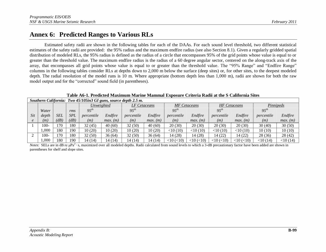
Programmatic EIS/OEIS
NSF & USGS Marine Seismic Research February 2011
Appendix B: B-99
Acoustic Modeling Report
Annex 6: Predicted Ranges to Various RLs
Estimated safety radii are shown in the following tables for each of the DAAs. For each sound level threshold, two different statistical estimates of the safety radii are provided: the 95% radius and the maximum endfire radius (see also Section 8.1). Given a regularly gridded spatial distribution of modeled RLs, the 95% radius is defined as the radius of a circle that encompasses 95% of the grid points whose value is equal to or
greater than the threshold value. The maximum endfire radius is the radius of a 60 degree angular sector, centered on the along-track axis of the
array, that encompasses all grid points whose value is equal to or greater than the threshold value. The ―95% Range‖ and ―Endfire Range‖
columns in the following tables consider RLs at depths down to 2,000 m below the surface (deep sites) or, for other sites, to the deepest modeled depth. The radial resolution of the model runs is 10 m. Where appropriate (bottom depth less than 1,000 m), radii are shown for both the raw
model output and for the ―corrected‖ sound field (in parentheses).
Table A6-1. Predicted Maximum Marine Mammal Exposure Criteria Radii at the S California Sites Southern California: Two 45/105in3 GI guns, source depth 2.5 m.
Sit
e
Water
depth
(m)
SEL
(dB)
rms
SPL
(dB)
Unweighted LF Cetaceans MF Cetaceans HF Cetaceans Pinnipeds
95th
percentile
(m)
Endfire
max. (m)
95th
percentile
(m)
Endfire
max. (m)
95th
percentile
(m)
Endfire
max. (m)
95th
percentile
(m)
Endfire
max. (m)
95th
percentile
(m)
Endfire
max. (m)
1 100-
1,000
170 180 32 (45) 40 (60) 32 (50) 40 (60) 20 (30) 20 (30) 20 (30) 20 (30) 30 (40) 30 (50)
180 190 10 (20) 10 (20) 10 (20) 10 (20) <10 (10) <10 (10) <10 (10) <10 (10) 10 (10) 10 (10)
2 100-
1,000
170 180 32 (50) 36 (64) 32 (50) 36 (64) 14 (28) 14 (28) 14 (22) 14 (22) 28 (36) 28 (42)
180 190 14 (14) 14 (14) 14 (14) 14 (14) <10 (<10) <10 (<10) <10 (<10) <10 (<10) <10 (14) <10 (14) Notes: SELs are in dB re μPa2 · s, maximized over all modeled depths. Radii calculated from sound levels to which a 3-dB precautionary factor have been added are shown in parentheses for shelf and slope sites.

Programmatic EIS/OEIS
NSF & USGS Marine Seismic Research February 2011
B-100 Appendix B: Acoustic Modeling Report
Table A6-2. Predicted Maximum Marine Mammal Exposure Criteria Radii at the Caribbean Sites Caribbean: Full 2-D refraction array, 36 guns (6,600 in
3), source depth 12 m.
Site
Water
depth (m)
SEL (dB)
rms
SPL (dB)
Unweighted LF Cetaceans MF Cetaceans HF Cetaceans Pinnipeds
95th
percentile (m)
Endfire max. (m)
95th
percentile (m)
Endfire max. (m)
95th
percentile (m)
Endfire max. (m)
95th
percentile (m)
Endfire max. (m)
95th
percentile (m)
Endfire max. (m)
1 <100 170 180 779 (1,142) 949 (1,379) 739 (1,120) 891 (1,338) 425 (533) 208 (366) 344 (447) 122 (258) 505 (815) 416 (524)
180 190 248 (348) 294 (380) 227 (340) 275 (366) 81 (117) 36 (50) 58 (81) 14 (36) 114 (262) 86 (150)
2 >1,00
0
170 180 696 806 632 741 232 133 182 112 326 245
180 190 218 252 199 226 71 20 61 10 102 71
3 100- 1,000
170 180 410 (524) 444 (517) 396 (508) 424 (495) 235 (342) 133 (206) 190 (257) 114 (165) 338 (446) 247 (332)
180 190 191 (238) 221 (272) 181 (228) 209 (260) 73 (104) 41 (51) 51 (82) 10 (41) 112 (149) 73 (114)
4 >1,00
0
170 180 694 802 632 738 234 131 180 95 326 244
180 190 214 247 197 229 72 36 58 23 102 72 Notes: SELs are in dB re μPa
2 ·
s, maximized over all modeled depths. Radii calculated from sound levels to which a 3-dB precautionary factor have been added are shown in parentheses for shelf and
slope sites.
Table A6-3. Predicted Maximum Marine Mammal Exposure Criteria Radii at the Galapagos Ridge Sites Galapagos Ridge: 2-D reflection array, 18 guns (3,300 in
3), source depth 6 m.
Site
Water
depth
(m)
SEL
(dB)
rms
SPL
(dB)
Unweighted LF Cetaceans MF Cetaceans HF Cetaceans Pinnipeds
95th
percentile
(m)
Endfire
max. (m)
95th
percentile
(m)
Endfire
max. (m)
95th
percentile
(m)
Endfire
max. (m)
95th
percentile
(m)
Endfire
max. (m)
95th
percentile
(m)
Endfire
max. (m)
1-0° >1,00
0
170 180 360 322 345 290 180 70 140 60 260 110
180 190 110 100 110 91 60 20 50 10 81 30
1-90° >1,00
0
170 180 357 323 345 290 180 70 140 60 260 110
180 190 110 95 110 90 60 20 50 10 81 30 Notes: SELs are in dB re μPa
2 ·
s, maximized over all modeled depths. Radii calculated from sound levels to which a 3-dB precautionary factor have been added are shown in parentheses for
shelf and slope sites.

Programmatic EIS/OEIS
NSF & USGS Marine Seismic Research February 2011
Appendix B: B-101
Acoustic Modeling Report
Table A6-4. Predicted Maximum Marine Mammal Exposure Criteria Radii at the W Gulf of Alaska Sites West Gulf of Alaska: 2-D reflection array, 18 guns (3,300 in
3), source depth 6 m.
Site
Water depth
(m)
SEL
(dB)
rms SPL
(dB)
Unweighted LF Cetaceans MF Cetaceans HF Cetaceans Pinnipeds
95th
percentile
(m)
Endfire
max. (m)
95th
percentile
(m)
Endfire
max. (m)
95th
percentile
(m)
Endfire
max. (m)
95th
percentile
(m)
Endfire
max. (m)
95th
percentile
(m)
Endfire
max. (m)
1 <100 170 180 788 (1,012) 301 (418) 773 (1,012) 288 (383) 357 (478) 95 (202) 225 (398) 54 (149) 459 (885) 202 (256)
180 190 165 (206) 98 (143) 166 (209) 89 (130) 63 (139) 14 (32) 45 (63) 10 (22) 139 (196) 32 (63)
2 100-1,000
170 180 383 (595) 320 (490) 364 (541) 288 (433) 180 (262) 67 (98) 143 (202) 54 (85) 266 (390) 117 (166)
180 190 108 (155) 89 (126) 104 (152) 82 (117) 54 (76) 14 (32) 45 (63) 10 (22) 76 (114) 32 (45)
3 >1,000 170 180 347 288 342 269 177 67 139 54 264 117
180 190 104 86 103 82 54 14 45 10 76 32
Notes: SELs are in dB re μPa2 · s, maximized over all modeled depths. Radii calculated from sound levels to which a 3-dB precautionary factor have been added are shown in parentheses for shelf and slope sites.
Table A6-5. Predicted Maximum Marine Mammal Exposure Criteria Radii at the NW Atlantic Sites NW Atlantic: Two 45/105 in
3 GI guns, source depth 2.5 m
Site
Water
depth
(m)
SEL
(dB)
rms
SPL
(dB)
Unweighted LF Cetaceans MF Cetaceans HF Cetaceans Pinnipeds
95th
percentile
(m)
Endfire
max. (m)
95th
percentile
(m)
Endfire
max. (m)
95th
percentile
(m)
Endfire
max. (m)
95th
percentile
(m)
Endfire
max. (m)
95th
percentile
(m)
Endfire
max. (m)
1 <100 170 180 36 (50) 42 (64) 36 (57) 42 (64) 20 (28) 14 (28) 14 (22) 14 (28) 28 (36) 28 (42)
180 190 14 (14) 14 (14) 14 (14) 14 (14) <10 (<10) <10 (<10) <10 (<10) <10 (<10) <10 (14) <10 (14)
2 100-1,000
170 180 36 (50) 42 (57) 32 (50) 36 (57) 14 (28) 14 (28) 14 (22) 14 (28) 28 (36) 28 (42)
180 190 14 (14) 14 (14) 14 (14) 14 (14) <10 (<10) <10 (<10) <10 (<10) <10 (<10) <10 (14) <10 (14)
3 >1,000 170 180 32 36 32 36 14 14 14 14 28 28
180 190 14 14 14 14 <10 <10 <10 <10 <10 <10
4 100-
1,000
170 180 32 (50) 36 (57) 32 (50) 36 (57) 14 (28) 14 (28) 14 (22) 14 (22) 28 (36) 28 (42)
180 190 14 (14) 14 (14) 14 (14) 14 (14) <10 (<10) <10 (<10) <10 (<10) <10 (<10) <10 (14) <10 (14)
Notes: SELs are in dB re μPa2 · s, maximized over all modeled depths. Radii calculated from sound levels to which a 3-dB precautionary factor have been added are shown in parentheses for shelf and slope sites.

Programmatic EIS/OEIS
NSF & USGS Marine Seismic Research February 2011
B-102 Appendix B:Acoustic Modeling Report
[This page intentionally left blank.]