appendix a menus, buttons, the mouse, and data flow978-1-84628-104-4/1.pdf · appendix a menus,...
TRANSCRIPT
Appendix A
Menus, Buttons, the Mouse, and Data Flow
Introduction
This appendix explains instructions on how to use the mouse. The explanation is followed by a description
of how data flows into, within, and out of an Object. This appendix concludes with the Object Order of
Operation sequence.
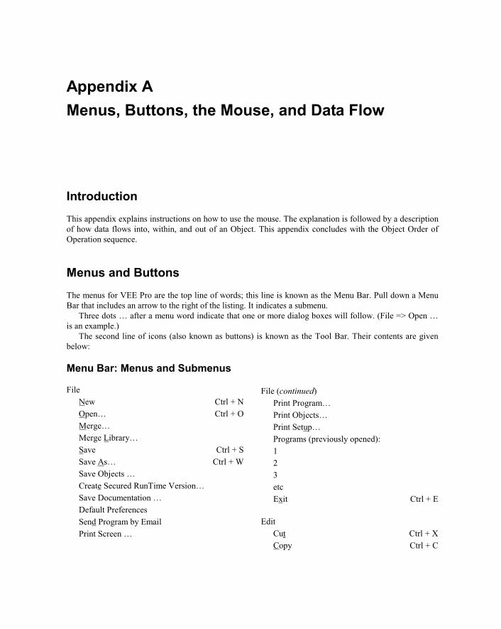
Menus and Buttons
The menus for VEE Pro are the top line of words; this line is known as the Menu Bar. Pull down a Menu
Bar that includes an arrow to the right of the listing. It indicates a submenu.
Three dots … after a menu word indicate that one or more dialog boxes will follow. (File => Open …
is an example.)
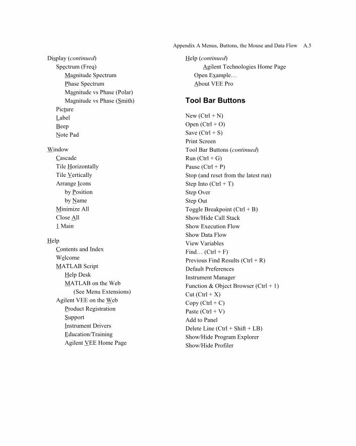
The second line of icons (also known as buttons) is known as the Tool Bar. Their contents are given
below:
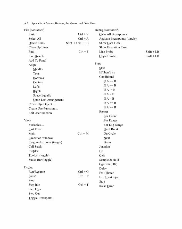
Menu Bar: Menus and Submenus
File
New Ctrl + N
Open… Ctrl + O
Merge…
Merge Library…
Save Ctrl + S
Save As… Ctrl + W
Save Objects …
Create Secured RunTime Version…
Save Documentation …
Default Preferences
Send Program by Email
Print Screen …
File (continued)
Print Program…
Print Objects…
Print Setup…
Programs (previously opened):
1
2
3
etc
Exit Ctrl + E
Edit
Cut Ctrl + X
Copy Ctrl + C
A.2 Appendix A Menus, Buttons, the Mouse, and Data Flow
File (continued)
Paste Ctrl + V
Select All Ctrl + A
Delete Lines Shift + Ctrl + LB
Clean Up Lines
Find… Ctrl + F
Find Results
Add To Panel
Align
Middles
Tops
Bottoms
Centers
Lefts
Rights
Space Equally
Undo Last Arrangement
Create UserObject…
Create UserFunction…
Edit UserFunction
View
Variables…
Last Error
Main Ctrl + M
Execution Window
Program Explorer (toggle)
Call Stack
Profiler
Toolbar (toggle)
Status Bar (toggle)
Debug
Run/Resume Ctrl + G
Pause Ctrl + P
Stop
Step Into Ctrl + T
Step Over
Step Out
Toggle Breakpoint
Debug (continued)
Clear All Breakpoints
Activate Breakpoints (toggle)
Show Data Flow
Show Execution Flow
Line Probe Shift + LB
Object Probe Shift + LB
Flow
Start
If/Then/Else
Conditional
If A == B
If A ~= B
If A != B
If A < B
If A > B
If A <= B
If A >= B
Repeat
For Count
For Range
For Log Range
Until Break
On Cycle
Next
Break
Junction
Do
Gate
Sample & Hold
Confirm (OK)
Delay
Exit Thread
Exit UserObject
Stop
Raise Error

Appendix A Menus, Buttons, the Mouse and Data Flow A.3
Device
Formula
MATLAB Script
Function & Object Browser Ctrl + l
UserObject
UserFunction
Call
Import Library
Delete Library
Sequencer
Virtual Source
Function Generator
Pulse Generator
Noise Generator
Regression
Counter
Accumulator
Timer
Shift Register
DeMultiplexer
Comparator
ActiveX Automation References…
ActiveX Control References…
ActiveX Controls (See Menu extensions)
I/O
Instrument Manager…
Advanced I/O
Interface Operations
Instrument Event
Interface Event
MultiInstrument Direct I/O
Bus I/O Monitor
To
File
DataSet
Printer
String
StdOut (UNIX)
StdErr (UNIX)
I/O; Bus I/O Monitor (continued)
From
File
DataSet
String
StdIn (UNIX)
To/From Named Pipe (UNIX)
To/From Socket
To/From DDE (PC)
Rocky Mountain Basic (UNIX)
Initialize Rocky M’tn Basic (UNIX)
To/From Rocky M’tn Basic (UNIX)
Execute Program (UNIX)
Execute Program (PC)
Print Screen
Data
Selection Control
Radio Buttons
Cyclic Button
List
Drop-Down List
Pop-Up List
Slider List
Toggle Control
Button
Check Box
Vertical Paddle
Horizontal Paddle
Vertical Rocker
Horizontal Rocker
Vertical Slide
Horizontal Slide
Dialog Box
Text Input
Int32 Input
Real64 Input
Message Box
List Box
File Name Selection

A.4 Appendix A Menus, Buttons, the Mouse, and Data Flow
Data (continued)
Continuous
Int32 Slider
ueal64 Slider
Int32 Knob
Real64 Knob
Constant
Text
UInt8
Int16
Int32
Real32
Real64
Coord
Complex
PComplex
Date/Time
Record
Variable
Set Variable
Get Variable
Delete Variable
Declare Variable
Build Data
Coord
Complex
PComplex
Waveform
Arb Waveform
Spectrum
Record
Unbuild Data
Coord
Complex
PComplex
Waveform
Spectrum
Record
Data (continued)
Allocate Array
Text
UInt8
Int16
Int32
Real32
Real64
Coord
Complex
PComplex
Access Array
uet Values
Get Values
Set Mappings
Get Mappings
Access Record
Merge Record
SubRecord
Set Field
Get Field
Concatenator
Sliding Collector
Collector
Display
AlphaNumeric
Logging AlphaNumeric
Indicator
Meter
Thermometer
Fill Bar
Tank
Color Alarm
XY Trace
Strip Chart
Complex Plane
X vs Y Plot
Polar Plot
Waveform (Time)
Appendix A Menus, Buttons, the Mouse and Data Flow A.5
Display (continued)
Spectrum (Freq)
Magnitude Spectrum
Phase Spectrum
Magnitude vs Phase (Polar)
Magnitude vs Phase (Smith)
Picture
Label
Beep
Note Pad
Window
Cascade
Tile Horizontally
Tile Vertically
Arrange Icons
by Position
by Name
Minimize All
Close All
1 Main
Help
Contents and Index
Welcome
MATLAB Script
Help Desk
MATLAB on the Web
(See Menu Extensions)
Agilent VEE on the Web
Product Registration
Support
Instrument Drivers
Education/Training
Agilent VEE Home Page
Help (continued)
Agilent Technologies Home Page
Open Example…
About VEE Pro
Tool Bar Buttons
New (Ctrl + N)
Open (Ctrl + O)
Save (Ctrl + S)
Print Screen
Tool Bar Buttons (continued)
Run (Ctrl + G)
Pause (Ctrl + P)
Stop (and reset from the latest run)
Step Into (Ctrl + T)
Step Over
Step Out
Toggle Breakpoint (Ctrl + B)
Show/Hide Call Stack
Show Execution Flow
Show Data Flow
View Variables
Find… (Ctrl + F)
Previous Find Results (Ctrl + R)
Default Preferences
Instrument Manager
Function & Object Browser (Ctrl + 1)
Cut (Ctrl + X)
Copy (Ctrl + C)
Paste (Ctrl + V)
Add to Panel
Delete Line (Ctrl + Shift + LB)
Show/Hide Program Explorer
Show/Hide Profiler

A.6 Appendix A Menus, Buttons, the Mouse, and Data Flow
Mouse Instructions
These instructions are for the left-hand mouse button:
This statement: means you should:
Click on an item Place the mouse pointer over the desired item and
press the left mouse button.
Double-click on an item Place the mouse pointer over the desired item and
press the left mouse button twice quickly.
Drag an item Place the mouse pointer over the desired item,
hold the left mouse button down, and move the
item to the appropriate location. Then, release the
mouse button.
The right-hand mouse button is to be depressed only when specifically noted in the text.
Programming
When solution steps for solving a decision portion of a program become complex, then it can first be
prepared as a flow chart or as pseudo code. Flow charts are either structured (single entry at the beginning
with a single exit at the end) or unstructured which consists of boxes connected by lines with multiple entry
and exit points. Pseudo code is programming-like notation, ranging from simple English words to
programming steps. A Pascal pseudo-code example for calculating interest is:
Pseudo Code Pascal
BEGIN PROGRAM SIMPLEINTEREST (OUTPUT);
Set the PRINCIPAL
amount invested at $620 VAR
Set the interest RATE at 0.075 (7.5%) PRINCIPAL, RATE, INTEREST, REAL;
Calculate the INTEREST as RATE *
PRINCIPAL BEGIN
WRITE the PRINCIPAL and
the interest RATE PRINCIPAL := 620;
WRITE the amount of
INTEREST earned RATE := 0.075;

Appendix A Menus, Buttons, the Mouse and Data Flow A.7
Pseudo Code (continued) Pascal (continued)
INTEREST := RATE * PRINCIPAL;
WRITELN (PRINCIPAL, RATE);
WRITELN (INTEREST)
END END.
VEE Pro Data Flow
Data flows from left to right through an object. On all the objects with data pins, the left data pins are
inputs and the right data pins are outputs.
All of an object’s data-input pins must be connected. Otherwise, an error will occur when the program
is run. If you do not wish to use them, then delete those pins.
An object will not execute until all of its data-input pins have received new data.
An object finishes executing only after all connected and appropriate data-output pins have been
activated.
You can change the order of execution by using sequence input and output pins. You do not normally
need to use these pins except to ensure the order of execution (when controlling external devices such as
instruments). Let data flow control the execution of your program.
Object Order of Operation
The order in which things happen within a VEE Pro object is:
1a. If the object’s Sequence Input pin is connected, then the object will wait for both the Data Input
and Sequence Input to receive data (or a ping) before it goes to step 2 below.

A.8 Appendix A Menus, Buttons, the Mouse, and Data Flow
1b. The object accepts data on its Data Input Pin(s). It will wait until there is data on all Data Input
Pins.
2. The object performs its designated function.
3. The object sends data out its Data Output Pin(s).
4. The object waits for a “receipt acknowledged” signal. The “receipt acknowledged” is then sent
when every object “down-thread” from this object has completed its operation.
5. The object sends its signal out its Sequence-Out pin.
The object then deactivates.

Appendix B
Partial Programming Sequences
Introduction
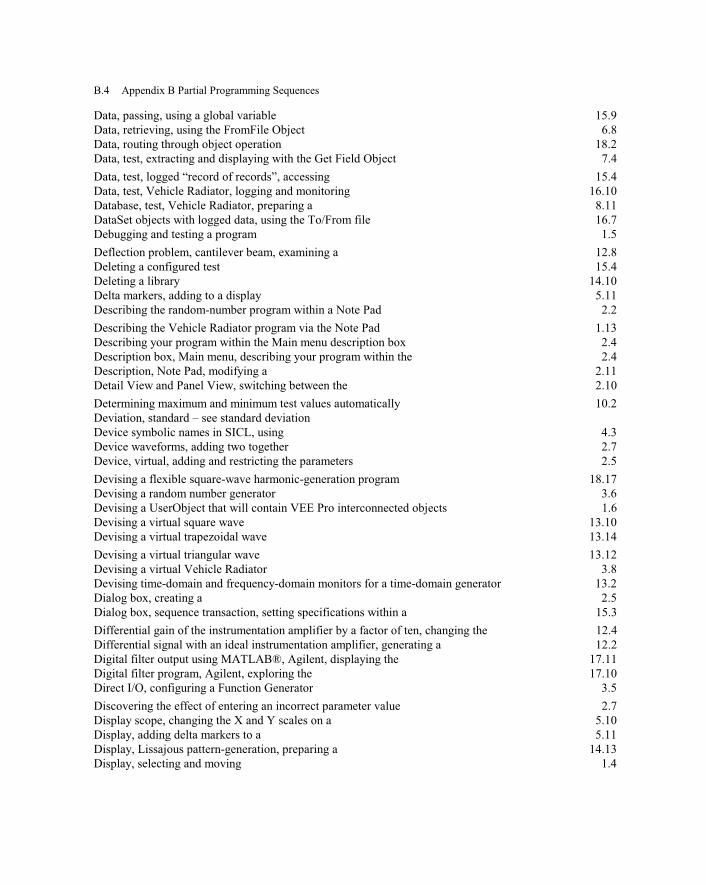
This appendix identifies those portions of programs that will help you during the preparation of your
programs. They are known as Partial Program Sequences. This is a different type of index; reference to
these portions of programs is listed alphabetically. Thus, you may quickly reference partial programs that
you use infrequently.
VEE Pro Subprograms
Subprogram Titles Lesson Page Number
34970A data acquisition switch unit, installing the 4.5
Access many picture files, using one UserFunction 18.15
Accessing logged “record of records” test data 15.4
Active instrument, sending a single text command to an 4.8
Active instrument, sending an expression list to an 4.8
ActiveX, sending VEE Pro data to an Excel™ spreadsheet via 9.2
Adding and restricting the parameters of a virtual device 2.5
Adding delta markers to a display 5.11
Adding or inserting a configured test 15.3
Adding two device waveforms together 2.7
Agilent digital filter output using MATLAB®, displaying the 17.11
Agilent digital filter program, exploring the 17.10
Alphanumeric display, monitoring a changing program with an 2.3
Alphanumeric displays, creating for displaying single or multiple values 2.14
Altering data in a specific record field with the Set Field Object 7.5
Analyzed, extracting a portion of the data to be 16.4
Analyzing several runs of data from the Sequencer 16.3
Angular deflection (torsion) of a round shaft, examining the 12.9

B.2 Appendix B Partial Programming Sequences
Applying I/O Transaction guidelines 14.4
Applying MATLAB example displays to a Vehicle Radiator program 12.15
Applying miscellaneous techniques and procedures to improve programs 18.11
Applying propagation rules to improve “auto execute” and “wait for input” 18.7
Applying techniques and guidelines that will assist in improving programs 18.5
Array, extracting values from 6.3
Array, real – see real array
Auto execute and “wait for input”, improve by applying propagation rules to 18.7
Background, panel, importing a bitmap for a 17.5
Bar chart, displaying VEE Pro data on a 11.2
Beam, cantilever deflection problem, examining a 12.8
Bitmap for a panel background, importing a 17.5
Box, dialog – see dialog box
Building a record 7.2
Building a Vehicle Radiator test record 16.10
Building the Vehicle Radiator operator interface 14.20
Calculating a ramp function using the Formula Object 5.5
Calculating standard deviation for a ramp function 5.6
Calculating two parameters using one Formula Object 5.4
Calculating various statistical parameters 6.10
Calculations, statistical, modifying the Vehicle Radiator program to include 7.9
Call Rand via an input terminal, setting up (three) tests in the Sequencer to 15.7
Calling a UserFunction from an expression 11.7
Calling a UserFunction from an expression 11.7
Cantilever beam deflection problem, examining a 12.8
Changing between Open View and Iconic View 1.4
Changing colors and fonts on an object 2.10
Changing colors on the panel 2.10
Changing object internal parameters 2.13
Changing object names to be more descriptive 2.13
Changing pin names to real-world label names 1.14
Changing program parameters via the Real Slider or Real Knob 2.7
Changing the color of a trace 5.12
Changing the differential gain of the instrumentation amplifier by a factor of ten 12.4
Changing the number of added cosine waves for a wave shape display 13.13
Changing the number of added sine waves for a wave shape display 13.11
Changing the number of combined cosine waves for a wave shape display 13.15
Changing the parameters within a program 1.10
Changing the X and Y scales on a display scope 5.10
Changing, selecting, moving, and values in a Virtual Source Object 1.3
Chart, bar – displaying VEE Pro data on a 11.2
Chart, strip – recording temperature readings on a 4.7
Clearing your Work Area and Opening the VEE Pro Program 1.2
Cloning, selecting, and modifying objects 2.3

Appendix B Partial Programming Sequences B.3
Coil spring, examining the natural frequency of a 12.10
Collector, using the 6.2
Color of a trace, changing 5.12
Colors and fonts, changing on an object 2.10
Colors, changing on the panel 2.10
Command, single text, sending to an active instrument 4.8
Comparing a waveform output with a mask 15.13
Concatenator, using the 6.4
Configured test, adding or inserting a 15.3
Configured test, deleting a 15.4
Configuring a Function Generator for Direct I/O 3.5
Configuring a virtual instrument to a real instrument 4.2
Configuring and specifying a pass/fail test 15.2
Configuring the interface 4.5
Connecting three objects within a UserObject area 1.8
Connecting two objects 1.4
Constructing a four-element simulated strain gauge 12.5
Contents of FromFile, examining the 2.15
Converting an object to an Iconic View, after selecting and editing 1.7
Correcting and stopping a program 1.15
Creating a dialog box 2.5
Creating a formula from within, after selecting a Function & Object Browser 1.7
Creating a high impact warning 17.7
Creating a status panel for an in-progress test 17.2
Creating a UserFunction 11.3
Creating a VEE Pro to Excel™ template 9.8
Creating a Vehicle Radiator operator interface 8.12
Creating a virtual thermometer 1.10
Creating Alphanumeric displays for displaying single or multiple values 2.14
Creating an operator interface 2.9
Creating an operator interface 8.10
Creating an XY trace with three inputs 5.8
Creating and merging a library of UserFunctions 14.2
Data acquisition switch unit, 34970A, installing the 4.5
Data from the Sequencer, analyzing several runs of 16.3
Data points, waveform, interpolating between 5.11
Data Set Object, storing a record from a 8.2
Data Set, retrieving and displaying a record from a 8.3
Data Sets, performing a search and sort operation with 8.6
Data to be analyzed, extracting a portion of the 16.4
Data via a UserFunction, passing, 15.7
Data, altering in a specific record field with the Set Field Object 7.5
Data, logged, using the To/From file DataSet objects with 16.7
Data, logged, using the To/From file objects with 16.5
B.4 Appendix B Partial Programming Sequences
Data, passing, using a global variable 15.9
Data, retrieving, using the FromFile Object 6.8
Data, routing through object operation 18.2
Data, test, extracting and displaying with the Get Field Object 7.4
Data, test, logged “record of records”, accessing 15.4
Data, test, Vehicle Radiator, logging and monitoring 16.10
Database, test, Vehicle Radiator, preparing a 8.11
DataSet objects with logged data, using the To/From file 16.7
Debugging and testing a program 1.5
Deflection problem, cantilever beam, examining a 12.8
Deleting a configured test 15.4
Deleting a library 14.10
Delta markers, adding to a display 5.11
Describing the random-number program within a Note Pad 2.2
Describing the Vehicle Radiator program via the Note Pad 1.13
Describing your program within the Main menu description box 2.4
Description box, Main menu, describing your program within the 2.4
Description, Note Pad, modifying a 2.11
Detail View and Panel View, switching between the 2.10
Determining maximum and minimum test values automatically 10.2
Deviation, standard – see standard deviation
Device symbolic names in SICL, using 4.3
Device waveforms, adding two together 2.7
Device, virtual, adding and restricting the parameters 2.5
Devising a flexible square-wave harmonic-generation program 18.17
Devising a random number generator 3.6
Devising a UserObject that will contain VEE Pro interconnected objects 1.6
Devising a virtual square wave 13.10
Devising a virtual trapezoidal wave 13.14
Devising a virtual triangular wave 13.12
Devising a virtual Vehicle Radiator 3.8
Devising time-domain and frequency-domain monitors for a time-domain generator 13.2
Dialog box, creating a 2.5
Dialog box, sequence transaction, setting specifications within a 15.3
Differential gain of the instrumentation amplifier by a factor of ten, changing the 12.4
Differential signal with an ideal instrumentation amplifier, generating a 12.2
Digital filter output using MATLAB®, Agilent, displaying the 17.11
Digital filter program, Agilent, exploring the 17.10
Direct I/O, configuring a Function Generator 3.5
Discovering the effect of entering an incorrect parameter value 2.7
Display scope, changing the X and Y scales on a 5.10
Display, adding delta markers to a 5.11
Display, Lissajous pattern-generation, preparing a 14.13
Display, selecting and moving 1.4

Appendix B Partial Programming Sequences B.5
Displaying a running program with a virtual oscilloscope 1.9
Displaying a waveform 5.10
Displaying a waveform 6.12
Displaying after retrieving a record from a Data Set 8.3
Displaying and extracting test data with the Get Field Object 7.4
Displaying the Agilent digital filter output using MATLAB® 17.11
Displaying the frequency and phase ratios for a Lissajous pattern 14.14
Displaying VEE Pro data on a bar chart 11.2
Displays, Alphanumeric, creating for displaying single or multiple values 2.14
Displays, applying MATLAB example to a Vehicle Radiator program 12.15
Document several test runs using Excel™ 10.9
Documenting your program 2.11
Editing a UserFunction 11.5
Editing a UserFunction 11.9
Editing after selecting an object and converting it to an Iconic View 1.7
Eliminating pins 2.13
Eliminating unneeded objects and pins and replacing objects 2.13
Evaluating a simple expression with the Formula Object 5.2
Examining a cantilever beam deflection problem 12.8
Examining a manufacturing test system program 12.12
Examining and interpreting a virtual scope waveform 2.11
Examining the ability of an IA to measure a small signal buried in noise 12.3
Examining the angular deflection (torsion) of a round shaft 12.9
Examining the contents of FromFile 2.15
Examining the contents of ToFile 2.9
Examining the natural convection of heat 12.11
Examining the natural frequency of a coil spring 12.10
Examining the use of the Note Pad via the Help menu 1.3
Excel™ spreadsheet via ActiveX, sending VEE Pro data to an 9.2
Excel™ spreadsheet, multi-column, preparing and transferring data to 10.5
Excel™ template, creating in VEE Pro 9.8
Excel™, using to document several test runs 10.9
Existing scope Panel Driver Object, reconfiguring 3.2
Existing scope Panel Driver Object, reconfiguring 3.2
Exploring the Agilent digital filter program 17.10
Expression list, sending to an active instrument 4.8
Expression, calling a UserFunction from an 11.7
Expression, calling a UserFunction from an 11.7
Expression, simple – evaluating with the Formula Object 5.2
Extracting a portion of the data to be analyzed 16.4
Extracting and displaying test data with the Get Field Object 7.4
Extracting values from an array 6.3
Extremes, temperature, Vehicle Radiator, monitoring and recording 16.9
Field, specific record, altering data with the Set Field Object 7.5

B.6 Appendix B Partial Programming Sequences
File – sending a time stamp to a 6.6
File name selection, using 14.7
File objects, To/From, using with logged data 16.5
File, DataSet objects, To/From, using with logged data 16.7
File, sending a real array to a 6.7
File, sending a text string to a 6.5
File, storing the program results using the ToFile Object 2.9
Finding functions in large programs 14.12
Fonts and colors, changing on an object 2.10
Forcing input parameters so the waveform stays within the Y axis scale 2.8
Formula Object, calculating a ramp function using the 5.5
Formula Object, calculating two parameters using one 5.4
Formula Object, evaluating a simple expression with the 5.2
Formula Object, multiline, preparing a 5.7
Formula Object, typing a function into 5.3
Formula, selecting a Function & Object Browser and creating a (formula) 1.7
Four-element simulated strain gauge, constructing a 12.5
Frequency and phase ratios for a Lissajous pattern, displaying the 14.14
Frequency-domain and time-domain monitors for a time-domain generator, devising 13.2
FromFile and ToFile Transactions, setting 2.13
FromFile Object, retrieving data using the 6.8
FromFile, examining the contents of 2.15
Function & Object Browser, selecting and creating a formula from within it 1.7
Function calls, icons and math arrays, refining VEE Pro Programs with 18.3
Function Generator, configuring for Direct I/O 3.5
Function, ramp – calculating standard deviation for 5.6
Function, ramp, calculating using the Formula Object 5.5
Function, typing into the Formula Object 5.3
Function, user – see UserFunction
Functions in large programs, finding 14.12
Generating a differential signal with an ideal instrumentation amplifier 12.2
Generator, Function – See Function Generator
Generator, random number, devising 3.6
Generator, time-domain, devising time-domain and frequency-domain monitors for a 13.2
Get Field Object – extracting and displaying test data with the 7.4
Global variable, passing data using a 15.9
Graph(s) and spreadsheet(s), transferring to Microsoft Word™ reports 10.11
Guidelines and techniques that will assist in improving programs, applying 18.5
Guidelines, I/O Transaction, applying 14.4
Harmonic-generation program, square-wave, devising a flexible 18.17
Heat, natural convection of, examining the 12.11
Help menu, examining the use of via the Note Pad 1.3
High impact warning, creating a 17.7
I/O Transaction guidelines, applying 14.4

Appendix B Partial Programming Sequences B.7
IA used to measure a small signal buried in noise, examining the ability of 12.3
Iconic View and Open View, changing between 1.4
Iconic View, selecting and editing an object and converting it to an 1.7
Icons, math arrays, and function calls, refining VEE Pro Programs with 18.3
Ideal instrumentation amplifier, generating a differential signal with an 12.2
Impact warning, high, creating a 17.7
Importing a bitmap for a panel background 17.5
Importing a library 14.10
Improve “auto execute” and “wait for input”, applying propagation rules to 18.7
Improve programs by applying miscellaneous techniques and procedures to 18.11
Improve programs, positioning Read/Write (sequential) Pointers to 18.9
Improve programs, using stopping loops to 18.8
Improving programs, applying techniques and guidelines that will assist in 18.5
Incorrect parameter value, discovering the effect of entering 2.7
In-progress test, creating a status panel for an 17.2
Input parameters, forcing so the waveform stays within the Y axis scale 2.8
Input terminal, via an, setting up (three) tests in the Sequencer to call Rand 15.7
Inputs, three, creating an XY trace with 5.8
Inserting or adding a configured test 15.3
Installing the 34970A data acquisition switch unit 4.5
Instrument, active – sending a single text command to 4.8
Instrument, active – sending an expression list to 4.8
Instrument, real– configuring from a virtual instrument 4.2
Instrument, virtual – configuring to a real instrument 4.2
Instrumentation Amplifier – also see IA
Instrumentation amplifier, changing the differential gain by a factor of ten 12.4
Instrumentation amplifier, ideal, generating a differential signal with an 12.2
Interconnected objects, devising a UserObject that will contain 1.6
Interface, configuring the 4.5
Interface, operator, creating an 2.9
Interface, operator, creating an 8.10
Interface, operator, securing an 8.14
Interface, operator, Vehicle Radiator, building the 14.20
Interface, operator, Vehicle Radiator, creating a 8.12
Interface, operator, Vehicle Radiator, securing the 14.22
Internal parameters, changing object 2.13
Interpolating between waveform data points 5.11
Interpreting and examining a virtual scope waveform 2.11
Label names (real-world), changing pin names to 1.14
Large programs, functions in, finding 14.12
Library of UserFunctions, creating and merging a 14.2
Library, deleting a 14.10
Library, importing a 14.10
Limits, test, Vehicle Radiator, modifying 16.10

B.8 Appendix B Partial Programming Sequences
Lissajous pattern, displaying the frequency and phase ratios for a 14.14
Lissajous pattern-generation display, preparing a 14.13
List, expression – sending to an active instrument 4.8
Logged “record of records” test data, accessing 15.4
Logged data, using the To/From file DataSet objects with 16.7
Logged data, using the To/From file objects with 16.5
Logging and monitoring Vehicle Radiator test data 16.10
Loops, stopping, using to improve programs 18.8
Main menu description box, describing your program within the 2.4
Manufacturing test system program, examining a 12.12
Markers, delta, adding to a display 5.11
Mask, comparing a waveform output with a 15.13
Math arrays, icons, and function calls, refining VEE Pro Programs with 18.3
MATLAB example displays to a Vehicle Radiator program, applying 12.15
MATLAB®, revising a virtual square wave via 13.16
MATLAB®, used to display the Agilent digital filter output 17.11
Maximum and minimum test values, determining automatically 10.2
Menu Bar, saving a program via 1.9
Menus, operator-interface, to guide an operator, using 16.13
Merging and creating a library of UserFunctions 14.2
Microsoft Word™ – see Word™
Minimum and maximum test values, determining automatically 10.2
Miscellaneous techniques and procedures to improve programs, applying 18.11
Modifying a Note Pad description 2.11
Modifying the Vehicle Radiator program to include statistical calculations 7.9
Modifying thermometer temperature-related parameters 1.11
Modifying Vehicle Radiator temperature-related parameters 1.13
Modifying Vehicle Radiator test limits 16.10
Modifying, selecting, and cloning objects 2.3
Monitoring a changing program with an alphanumeric display 2.3
Monitoring and logging Vehicle Radiator test data 16.10
Monitoring and recording Vehicle Radiator temperature extremes 16.9
Monitoring the thermometer UserObject 1.11
Monitoring the Vehicle Radiator UserObject 1.13
Monitors, devising time-domain and frequency-domain for a time-domain generator 13.2
Mouse right button, selecting Properties with your 1.7
Moving and selecting a display 1.4
Moving, selecting, and changing values in a Virtual Source Object 1.3
Moving, selecting, and sizing a Note Pad Object 1.2
Multi-column Excel™ spreadsheet, preparing and transferring data to a 10.5
Multi-line Formula Object, preparing a 5.7
Multiple or single values, creating Alphanumeric displays for displaying 2.14
Natural convection of heat, examining the 12.11
Natural frequency of a coil spring, examining the 12.10

Appendix B Partial Programming Sequences B.9
Noise, examining the ability of an IA to measure a small signal buried in 12.3
Note Pad description, modifying a 2.11
Note Pad Object, selecting, moving, and sizing 1.2
Note Pad, describing the random-number program within a 2.2
Note Pad, describing the Vehicle Radiator program 1.13
Note Pad, examining the use of via the Help menu 1.3
Number of added cosine waves for a wave shape display, changing the 13.13
Number of added sine waves for a wave shape display, changing the 13.11
Number of combined cosine waves for a wave shape display, changing the 13.15
Numbers, real – see real numbers
Object component parts, selecting the program of 1.14
Object names, changing to be more descriptive 2.13
Object operation, routing data through 18.2
Object, changing colors and fonts on an 2.10
Object, changing internal parameters 2.13
Object, Data Set, storing a record from 8.2
Object, Formula, evaluating a simple expression with the 5.2
Object, Formula, calculating a ramp function using the 5.5
Object, Formula, calculating two parameters using one 5.4
Object, Formula, preparing a multi-line 5.7
Object, Formula, typing a function into 5.3
Object, FromFile, retrieving data using the 6.8
Object, Get Field, extracting and displaying test data with the 7.4
Object, reconfiguring an existing scope Panel Driver 3.2
Object, selecting and editing, and converting it to an Iconic View 1.7
Object, Set Field, altering data in a specific record field with 7.5
Objects and pins, eliminating unneeded and replacing 2.13
Objects, (three) connecting within a UserObject area 1.8
Objects, connecting two 1.4
Objects, DataSet file, To/From, using with logged data 16.7
Objects, file, To/From, using with logged data 16.5
Objects, interconnected, devising a UserObject that will contain 1.6
Objects, selecting, cloning, and modifying 2.3
Observing the effect of parameter changes to the thermometer program 1.11
Observing the effect of parameter changes to the Vehicle Radiator program 1.14
Open View and Iconic View, changing between 1.4
Opening the VEE Pro Program and clearing your Work Area 1.2
Operation, object, routing data through 18.2
Operation, search and sort, performing with Data Sets 8.6
Operation, search, preparing for a 8.8
Operator interface, creating an 2.9
Operator interface, creating an 8.10
Operator interface, securing an 8.14
Operator interface, Vehicle Radiator, building the 14.20
B.10 Appendix B Partial Programming Sequences
Operator interface, Vehicle Radiator, creating a 8.12
Operator interface, Vehicle Radiator, securing the 14.22
Operator, using operator-interface menus to guide an 16.13
Operator-interface menus to guide an operator, using 16.13
Oscilloscope, – also see Waveform (Time)
Oscilloscope, virtual, displaying a running program with a 1.9
Output waveform, comparing with a mask 15.13
Panel background, bitmap for a, importing 17.5
Panel View and Detail View, switching between the 2.10
Panel, changing colors on the 2.10
Panel, status, for an in-progress test, creating a 17.2
Parameter changes, observing the effect in the thermometer program 1.11
Parameter changes, observing the effect on the Vehicle Radiator program 1.14
Parameter value, incorrect, discovering the effect of entering 2.7
Parameters of a program, varying the 2.6
Parameters of a virtual device, adding and restricting the 2.5
Parameters, changing within a program 1.10
Parameters, input, forcing so the waveform stays within the Y axis scale 2.8
Parameters, internal, changing object 2.13
Parameters, program, changing via the Real Slider or Real Knob 2.7
Parameters, statistical – see statistical parameters
Parameters, temperature-related, modifying thermometer 1.11
Parameters, two, calculating using one Formula Object 5.4
Pass/fail test, configuring and specifying a 15.2
Passing data using a global variable 15.9
Passing data via a UserFunction 15.7
Pattern, Lissajous, displaying the frequency and phase ratios for a 14.14
Pattern-generation display, Lissajous, preparing a 14.13
Performing a search and sort operation with Data Sets 8.6
Phase and frequency ratios for a Lissajous pattern, displaying the 14.14
Picture files, using one UserFunction to access many 18.15
Pin names, changing to real-world label names 1.14
Pins and objects, eliminating unneeded and replacing 2.13
Pointers (sequential), Read/Write positioning to improve programs 18.9
Points, waveform data, interpolating between 5.11
Positioning Read/Write (sequential) Pointers to improve programs 18.9
Preparing a Lissajous pattern-generation display 14.13
Preparing a multiline Formula Object 5.7
Preparing a Vehicle Radiator test database 8.11
Preparing and transferring data to a multicolumn Excel™ spreadsheet 10.5
Preparing for a search operation 8.8
Printing a VEE Pro screen 2.11
Printing reports in Microsoft Word™ 9.15
Procedures and techniques, miscellaneous, to improve programs, applying 18.11

Appendix B Partial Programming Sequences B.11
Program parameters, changing via the Real Slider or Real Knob 2.7
Program results, storing the, in a file using the ToFile Object 2.9
Program, changing the parameters within 1.10
Program, changing, monitoring with an alphanumeric display 2.3
Program, describing your, within the Main menu description box 2.4
Program, devising a flexible square-wave harmonic-generation 18.17
Program, displaying with a virtual oscilloscope 1.9
Program, documenting your 2.11
Program, Opening and clearing your Work Area 1.2
Program, random-number, describing within a Note Pad, 2.2
Program, saving a 1.5
Program, saving via the Menu Bar 1.9
Program, selecting object component parts 1.14
Program, stopping and correcting a 1.15
Program, testing and debugging a 1.5
Program, varying the parameters 2.6
Program, Vehicle Radiator – see Vehicle Radiator program
Program, Vehicle Radiator, applying MATLAB example displays to a 12.15
Programs (large), functions in, finding 14.12
Programs, improve by applying miscellaneous techniques and procedures to 18.11
Programs, improve, positioning Read/Write (sequential) Pointers to 18.9
Programs, improve, using stopping loops to 18.8
Programs, improving, applying techniques and guidelines that will assist in 18.5
Programs, VEE Pro, refining with math arrays, icons, and function calls 18.3
Propagation rules to improve “auto execute” and “wait for input”, applying 18.7
Properties, selecting with your mouse right button 1.7
PulseProgram, revising to allow Vehicle Radiator simulation 2.12
Ramp function, calculating standard deviation for a 5.6
Ramp function, calculating using the Formula Object 5.5
Rand, call, via an input terminal, setting up (three) tests in the Sequencer to 15.7
Random number generator, devising a 3.6
Random-number program, describing the, within a Note Pad 2.2
Ratios, frequency and phase, for a Lissajous pattern, displaying the 14.14
Read/Write (sequential) Pointers positioning to improve programs 18.9
Real array, sending to a file 6.7
Real instrument – configuring from a virtual instrument 4.2
Real Knob or Real Slider, changing program parameters via the 2.7
Real numbers, storing 6.9
Real Slider or Real Knob, changing program parameters via the 2.7
Reconfiguring an existing scope Panel Driver Object 3.2
Record field, specific, altering data with the Set Field Object 7.5
Record of records, logged test data, accessing 15.4
Record, building a 7.2
Record, retrieving and displaying from a Data Set 8.3

B.12 Appendix B Partial Programming Sequences
Record, storing from a Data Set Object 8.2
Record, test, building a Vehicle Radiator, 16.10
Record, unbuilding in a single step 7.7
Recording and Monitoring Vehicle Radiator temperature extremes 16.9
Recording several Vehicle Radiator tests 14.16
Recording temperature readings on a strip chart 4.7
Refining VEE Pro Programs with math arrays, icons, and function calls 18.3
Replacing objects and eliminating pins 2.13
Reports, printing in Word™ 9.15
Restricting and adding the parameters of a virtual device 2.5
Retrieving and displaying a record from a Data Set 8.3
Retrieving data using the FromFile Object 6.8
Revising a virtual square wave via MATLAB® 13.16
Revising PulseProgram to allow Vehicle Radiator simulation 2.12
Round shaft, examining the angular deflection (torsion) of a 12.9
Routing data through object operation 18.2
Rules, propagation, to improve “auto execute” and “wait for input”, applying 18.7
Runs of data from the Sequencer, analyzing several 16.3
Saving a program via the Menu Bar 1.9
Saving a program 1.5
Scale, Y axis, forcing input parameters so the waveform stays within 2.8
Scope, display, changing the X and Y scales on a 5.10
Scope, existing Panel Driver Object, reconfiguring 3.2
Scope, virtual waveform, examining and interpreting a 2.11
Search and sort operation, performing with Data Sets 8.6
Search operation, preparing for a 8.8
Securing an operator interface 8.14
Securing the Vehicle Radiator operator interface 14.22
Selecting a Function & Object Browser and creating a formula from within it 1.7
Selecting and editing an object and converting it to an Iconic View 1.7
Selecting and moving a display 1.4
Selecting program object component parts 1.14
Selecting Properties with your mouse right button 1.7
Selecting, cloning, and modifying objects 2.3
Selecting, moving, and changing values in a Virtual Source Object 1.3
Selecting, moving, and sizing a Note Pad Object 1.2
Selection, using file name 14.7
Sending a real array to a file 6.7
Sending a single text command to an active instrument 4.8
Sending a text string to a file 6.5
Sending a time stamp to a file 6.6
Sending an expression list to an active instrument 4.8
Sending VEE Pro data to an Excel™ spreadsheet via ActiveX 9.2
Sequence transaction dialog box, setting specifications within a 15.3

Appendix B Partial Programming Sequences B.13
Sequencer to call Rand via an input terminal, setting up (three) tests in the 15.7
Sequencer, analyzing several runs of data from the 16.3
Set Field Object, altering data in a specific record field with the 7.5
Setting specifications within a sequence transaction dialog box 15.3
Setting ToFile and FromFile Transactions 2.13
Setting up (three) tests in the Sequencer to call Rand via an input terminal 15.7
SICL, using device symbolic names in 4.3
Signal (small) buried in noise, examining the ability of an IA to measure 12.3
Simulated strain gauge, four-element, constructing a 12.5
Simulating a Vehicle Radiator whose temperature varies linearly 1.12
Simulation, Vehicle Radiator, revising PulseProgram to allow 2.12
Sine waves, added, changing the number for a wave shape display 13.11
Single or multiple values, creating Alphanumeric displays for displaying 2.14
Single text command, sending to an active instrument 4.8
Sizing, selecting, and moving a Note Pad Object 1.2
Sort with Data Sets after the search operation 8.6
Specific record field, altering data with the Set Field Object 7.5
Specifications within a sequence transaction dialog box, setting 15.3
Specifying and configuring a pass/fail test 15.2
Spreadsheet – see Excel™ spreadsheet
Spreadsheet(s) and graph(s), transferring to Microsoft Word™ reports 10.11
Square wave via MATLAB®, revising a virtual 13.16
Square wave, devising a virtual 13.10
Square-wave harmonic-generation program, devising a flexible 18.17
Stamp, time – see time stamp
Standard deviation, calculating for a ramp function 5.6
Statistical calculations, modifying the Vehicle Radiator program to include 7.9
Statistical parameters, calculating various 6.10
Status panel for an in-progress test, creating a 17.2
Stopping and correcting a program 1.15
Stopping loops, using to improve programs 18.8
Storing a record from a Data Set Object 8.2
Storing real numbers 6.9
Storing the program results in a file using the ToFile Object 2.9
Storing the time stamp 6.9
Strain gauge, four-element simulated, constructing a 12.5
String, text – see text string
Strip chart, recording temperature readings on a 4.7
Switching between the Panel View and Detail View 2.10
Symbolic names, device, in SICL, using 4.3
Techniques and guidelines that will assist in improving programs, applying 18.5
Techniques and procedures, miscellaneous, to improve programs, applying 18.11
Temperature extremes, Vehicle Radiator, monitoring and recording 16.9
Temperature readings on a strip chart, recording 4.7

B.14 Appendix B Partial Programming Sequences
Temperature varies linearly, Vehicle Radiator simulation 1.12
Temperature-related parameters, modifying thermometer 1.11
Temperature-related parameters, modifying Vehicle Radiator 1.13
Terminal, input, via an, setting up (three) tests in the Sequencer to call Rand 15.7
Test data, extracting and displaying with the Get Field Object 7.4
Test data, logged “record of records”, accessing 15.4
Test data, Vehicle Radiator, logging and monitoring 16.10
Test database, Vehicle Radiator, preparing 8.11
Test limits, Vehicle Radiator, modifying 16.10
Test record, building a Vehicle Radiator 16.10
Test runs, using Excel™ to document several 10.9
Test values, maximum and minimum, determining automatically 10.2
Test, configured, adding or inserting a 15.3
Test, configured, deleting a 15.4
Test, in-progress, creating a status panel for an 17.2
Test, manufacturing system program, examining a 12.12
Test, pass/fail, configuring and specifying a 15.2
Testing and debugging a program 1.5
Tests (three) in the Sequencer to call Rand via an input terminal, setting up 15.7
Tests, Vehicle Radiator, recording several 14.16
Text string, sending to a file 6.5
Thermometer program, observing the effect of parameter changes 1.11
Thermometer, modifying temperature-related parameters 1.11
Thermometer, monitoring the UserObject 1.11
Thermometer, virtual, creating a 1.10
Time stamp, sending to a file 6.6
Time stamp, storing the 6.9
Time-domain and frequency-domain monitors for a time-domain generator, devising 13.2
Time-domain generator, devising time-domain and frequency-domain monitors for a 13.2
To/From file DataSet objects with logged data, using the 16.7
To/From file objects with logged data, using the 16.5
ToFile and FromFile Transactions, setting 2.13
ToFile Object, storing the program results in a file using 2.9
ToFile, examining the contents of 2.9
Torsion (angular deflection) of a round shaft, examining the 12.9
Trace, changing the color of a 5.12
Trace, XY – see XY trace
Transaction guidelines, I/O, applying 14.4
Transaction, sequence – see sequence transaction
Transactions, setting ToFile and FromFile 2.13
Transferring spreadsheet(s) and graph(s) to Microsoft Word™ reports 10.11
Transferring VEE Pro data into a Microsoft Word™ document 9.9
Transferring, after preparing data for a multicolumn Excel™ spreadsheet 10.5
Trapezoidal wave, devising a virtual 13.14

Appendix B Partial Programming Sequences B.15
Triangular wave, devising a virtual 13.12
Typing a function into the Formula Object 5.3
Unbuilding a record in a single step 7.7
UserFunction from an expression, calling a 11.7
UserFunction from an expression, calling a 11.7
UserFunction to access many picture files, using one 18.15
UserFunction, creating a 11.3
UserFunction, editing a 11.5
UserFunction, editing a 11.9
UserFunction, passing data via a 15.7
UserFunctions, library of, creating and merging a 14.2
UserObject area, connecting three objects within a 1.8
UserObject, devising one that will contain VEE Pro interconnected objects 1.6
UserObject, monitoring the thermometer 1.11
UserObject, monitoring the Vehicle Radiator 1.13
Using a global variable, passing data 15.9
Using device symbolic names in SICL 4.3
Using Excel™ to document several test runs 10.9
Using file name selection 14.7
Using one UserFunction to access many picture files 18.15
Using operator-interface menus to guide an operator 16.13
Using stopping loops to improve programs 18.8
Using the collector 6.2
Using the Concatenator 6.4
Using the To/From file DataSet objects with logged data 16.7
Using the To/From file objects with logged data 16.5
Value, incorrect parameter, discovering the effect of entering 2.7
Values from an array, extracting 6.3
Values, single or multiple, creating Alphanumeric displays for displaying 2.14
Variable, global, passing data using a 15.9
Varying the parameters of a program 2.6
VEE Pro data into a Word™ document, transferring 9.9
VEE Pro data on a bar chart, displaying 11.2
VEE Pro data, sending to an Excel™ spreadsheet via ActiveX 9.2
VEE Pro Excel™ template, creating a 9.8
VEE Pro Programs, refining with math arrays, icons, and function calls 18.3
VEE Pro screen, printing a, 2.11
Vehicle Radiator operator interface, building the 14.20
Vehicle Radiator operator interface, creating a 8.12
Vehicle Radiator operator interface, securing the 14.22
Vehicle Radiator program, applying MATLAB example displays to a 12.15
Vehicle Radiator program, describing via the Note Pad 1.13
Vehicle Radiator program, modifying to include statistical calculations 7.9
Vehicle Radiator program, observing the effect of parameter changes 1.14

B.16 Appendix B Partial Programming Sequences
Vehicle Radiator simulation, revising PulseProgram to allow 2.12
Vehicle Radiator temperature extremes, monitoring and recording 16.9
Vehicle Radiator temperature-related parameters, modifying 1.13
Vehicle Radiator test data, logging and monitoring 16.10
Vehicle Radiator test database, preparing a 8.11
Vehicle Radiator test limits, modifying 16.10
Vehicle Radiator test record, building a 16.10
Vehicle Radiator tests, recording several 14.16
Vehicle Radiator UserObject, monitoring the 1.13
Vehicle Radiator, simulating where a temperature varies linearly 1.12
Vehicle Radiator, virtual, devising 3.8
Views, Panel and Detail, switching between the 2.10
Virtual device, adding and restricting the parameters of a 2.5
Virtual instrument, configuring to a real instrument 4.2
Virtual scope waveform, examining and interpreting a 2.11
Virtual Source Object, selecting, moving, and changing values 1.3
Virtual square wave via MATLAB®, revising a 13.16
Virtual Vehicle Radiator, devising 3.8
Wait for input and “auto execute”, improve by applying propagation rules to 18.7
Warning, high impact, creating a 17.7
Wave shape display, changing the number of added cosine waves for a 13.13
Wave shape display, changing the number of added sine waves for a 13.11
Wave shape display, changing the number of combined cosine waves for a 13.15
Wave, square, devising a virtual 13.10
Wave, trapezoidal, devising a virtual 13.14
Wave, triangular, devising a virtual 13.12
Waveform (Time) – also see Oscilloscope
Waveform data points, interpolating between 5.11
Waveform output with a mask, comparing a 15.13
Waveform, displaying a 5.10
Waveform, displaying a 6.12
Waveform, forcing input parameters to stay within the Y axis scale 2.8
Waveform, virtual scope, examining and interpreting a 2.11
Waveform, zooming in on part of 5.10
Waveforms, device, adding two together 2.7
Word™ document, transferring VEE Pro data into 9.9
Word™ reports, transferring spreadsheet(s) and graph(s) to 10.11
Word™, printing reports in 9.15
Work Area, clearing; and Opening the VEE Pro Program 1.2
X and Y scales, changing on a display scope 5.10
XY trace, creating with three inputs 5.8
Y and X scales, changing on a display scope 5.10
Y axis scale, forcing input parameters so the waveform stays within 2.8
Zooming in on part of a waveform 5.10

Appendix C
Virtual Devices and Instruments
Introduction
This appendix presents the characteristics of the VEE Pro virtual devices and instruments available within
VEE Pro. For each of these items, a summary of their “help” menus is given.
Table of Contents Page Number
Devices C.2
The Formula C.2
The Function & Object Browser C.2
The UserObject C.4
The UserFunction C.5
The Sequencer C.5
Virtual Sources C.6
The Function Generator C.6
The Pulse Generator C.6
The Noise Generator C.6
Other Devices C.6
Regression C.6
Counter C.7
Accumulator C.7
Timer C.7
Shift Register C.7
DeMultiplexer C.7
Comparator C.7
ActiveX Automation References… C.8
ActiveX Control References… C.8
Displays C.9
AlphaNumeric C.9
Logging AlphaNumeric C.9

C.2 Appendix C Virtual Devices and Instruments
Table of Contents (continued) Page Number
Indicators C.9
Meter C.9
Thermometer C.9
Fill Bar C.9
Tank C.9
Color Alarm C.10
XY Trace C.10
Strip Chart C.10
Complex Plane C.10
X to Y Plot C.10
Polar Plot C.10
Waveform (Time) C.10
Spectrum (Freq) C.11
Magnitude Spectrum C.11
Phase Spectrum C.11
Magnitude vs. Phase (Polar) C.11
Magnitude vs. Phase (Smith) C.11
Picture C.11
Label C.12
Beep C.12
Note Pad C.12
Devices
The Formula Object performs an arithmetic multiplication on two operands by using a*b to multiply the
values of two input containers (terminals or pins) labeled: a and b. These containers may be of any type or
shape. If one of the containers is an array, then the other must be either a scalar or an array of the same size
and shape. The result is a container of the highest type, with the same shape as the operands. If both
operands are of type Coord, then they must have their independent variable(s) match exactly. Otherwise, an
error is returned. The multiplication is only performed on the dependent (last) variable. If one of the
containers is Text, then the other must be an Int32. Text multiplication consists of repeating the string the
number of times given by the value of Int32. Enums are converted to Text for multiplication. This
multiplication operation performs a parallel multiplication on all elements of the arrays, including matrices.
For a matrix multiply, see the function matMultiply(A,B). For detailed information, see the Formula Help
dialog box.
The Menu Bar => Device => Function & Object Browser contains an enormous number of selections, such
as:
Type
Operators
Built-in Functions
MATLAB® Functions
Local User Functions

Appendix C Virtual Devices and Instruments C.3
Imported User Functions
Remote User Functions
Compiled Functions
ActiveX Objects
VEE Objects
Instruments
Category
<All>
ActiveX Automation
Array
Bessel
Bitwise
Calculus
Complex Parts
Data Filtering
Generate
Matrix
Panel
Power
Probability & Statistics
Real Parts
Signal Processing
String
System Information
Time & Date
Trig
Type Conversion
For Built-in Functions; Category – <All>: The available Functions are:
abs acos acosh acot acoth
Aj asComplex asCoord asin asinh
asInt16 asInt32 asPComplex asReal32 asReal64
asText asUInt8 asVariant asVariantBool asVariantCurrency
asVariantDate asVariantEmpty asVariantError asVariantNull atan
atan2 atanh bartlet baseName beta
Bi binomial bit bitAnd bitCmpl
bitOr bits bitShift bitXor blackman
ceil charToint clearBit clipLower clipUpper
cofactor comb commandLine concat conj
convolve cos cosh cot coth
CreateObject cubert defIntegral deriv derivAt

C.4 Appendix C Virtual Devices and Instruments
det dirName dmyToDate erf erfc
errorinfo exp exp10 factorial fft
floor fracPart gamma getEnv getHostname
GetObject hamming hanning help hidePanel
hmsToHour hmsToSec i0 i1 identity
ifft im inDaylightSavings init installDir
integral intPart intToChar inverse
isVariant isVariantBool isVariantCurrency isVariantDate isVariantEmpty
isVariantError isVariantNull j j0 j1
jn k0 k1 lockPosition log
log10 logMagDist logRamp mag magDist
matDivide matMultiply max maxindex maxX
mday mean meanSmooth median min
minIndex minor minX mode Month
movingAvg now ordinal panelPosition panelSize
perm phase poly polySmooth product
programName ramp random randomize randomSeed
re recip rect rms rotate
round savePanelImage sdev setBit showPanel
signof sin sinh sort sq
sqrt strDown strFromLen strFromThru strLen
strPosChar strPosStr strRev strTrim strUp
sum tan tanh totSize transpose
typeName unlockPosition vari wday whichOS
whichPlatform whichVersion xcorrelate xlogRamp xramp
y0 y1 year yn
See: “The Function & Object Browser Help” dialog box for each of the above selections.
The UserObject is an object that may contain other objects. It is used to logically and physically group
objects together. It constitutes a separate “context” from the root context of a program. Multiple
UserObjects may be nested within a program. Create a UserObject by moving other objects into the work
area of the Open View of that UserObject (or select objects and use Menu Bar => Edit => Create
UserObject). The Make UserFunction item in the Object menu allows you to convert the UserObject into a
UserFunction. That UserFunction can then be called using the Call Function Object or from certain
expressions. No objects inside of a UserObject will operate until all data inputs to the UserObject are

Appendix C Virtual Devices and Instruments C.5
activated. All operations inside of the UserObject must be completed before the data outputs are activated.
When objects inside the UserObject are connected to objects outside the UserObject, data-input pins and
data-output pins are automatically created whenever Create UserObject is selected. Add data-input pins and
data-output pins to existing UserObjects using Add Terminal from the Object menu. The right mouse button
will provide a pop-up menu when the pointer is over an object within the UserObject. Additional
information is given in the UserObject Help dialog box.
The UserFunction is created empty from Menu Bar => Device => UserFunction or converted from a
UserObject by executing Make UserFunction. You can also create a UserFunction by selecting a group of
objects and using Menu Bar => Edit => Create UserFunction. Edit UserFunction will allow you to edit the
UserFunction once it has been created. UserFunctions exist in the “background” and can be called with Call
Function or from certain expressions. The UserFunction will have the same functionality as the
UserObject(s). When you convert a UserObject to a UserFunction, the UserObject will disappear from the
screen and will be replaced with a Call Function Object containing a call to the new UserFunction and the
new UserFunction window. The UserFunction will be added to the list of available UserFunctions that exist
in the “background” within the program. You can call the UserFunction using the Call Function Object, or
from certain expressions. You can edit the UserFunction by using Menu Bar => Edit => Edit UserFunction
or by double-clicking on it from the Program Explorer.
The Sequencer is a transaction-based object. It has program-development benefits that include:
• easy development of a test plan,
• a wide array of branching capabilities between tests,
• major components for building a customized test executive,
• the ability to call tests in VEE Pro and other languages, and
• automatic logging of test results.
More information is available from the (Test) Sequencer Help menu. The Sequencer is a very powerful
object that can also do simple operations well.
The Sequencer Object executes tests in a specified order based upon previous or programmed results. Each
test may be
• a VEE Pro User Function,
• a Compiled Function,
• a Remote Function that returns a single result, or
• any expression or a combination of the above functions calls in an expression.
Several variable names are also available, such as “thisTest” to correspond to the currently executing text.
Also, the name of each test that has already been executed is available as a record, such as “test1.Pass”.
That result is compared to a test specification to determine whether or not it has passed pre-established
criteria. This result can also be an expression or a function call. The Sequencer then uses a pass-or-fail

C.6 Appendix C Virtual Devices and Instruments
indicator to determine the next test it should perform. More information is available from the (Test)
Sequencer Help menu.
The options for branching to the next test are:
• executing the next test,
• repeating the same test, or
• jumping back to an earlier test.
The Sequencer can ask for user input to decide the appropriate course of action. As a test-sequence
developer, you can specify the order of tests. Then you can instruct your program to branch to a different
test based upon an analysis of your previously completed tests.
After the specified tests have been executed, the Sequencer automatically logs the test data to an output
terminal. The specific field log can be customized in the Object properties. The data can then be analyzed
and displayed. It can also be stored in a file, such as a server file, for later analysis.
Virtual Sources
The Virtual Source icon contains a Function Generator, Pulse Generator, and a Noise Generator. (See Menu
Bar => Device => Virtual Source.)
The Function Generator Object is used to simulate repetitive waveforms. It will provide sine, cosine, square,
triangle, +ramp, and -ramp waveforms as well as a simple Dc (horizontal) line. It will allow you to vary the
waveform frequency, amplitude, Dc Offset, phase, time span, and number of points in the display.
The Pulse Generator Object is used to simulate pulses. It will allow you to vary the pulse frequency, width,
delay, thresholds, rise time, fall time, pulse high value, and pulse low value. It also contains a Burst mode
whose burst count, repetition rate, time span and number of points in the display can be varied.
The Noise Generator Object is used to simulate noise that can be added to a waveform. Its amplitude, time
span, and number of points in the display can be varied.
Other Devices
The Regression Object is used to fit a linear regression line to (x,y) data. It uses the linear regression to fit a
straight line to the data using the equation
y = c0 + c1*x
where x is the x coordinate, and c0 and c1 are calculated coefficients. This type of regression should be
thought of as fitting the best straight line through the data. The (linear) Regression Object expects an array
of Coord type of input with one independent variable – an (x,y) pair
• If the input array is not a Coord type, then an attempt is made to convert it to Coord.
• If the input data are mapped (Waveform, Spectrum, or a mapped array), then the conversion to
Coord uses the mapping information to create the x part of the (x,y) pairs.

Appendix C Virtual Devices and Instruments C.7
• If the input data are not mapped (example: an array), then the x part of the (x,y) pair is implicitly
generated from its position in the array.
The Fit Type field on the open view is used to change the regression type to linear, logarithmic, exponential,
power curve, or polynomial regression. Click on the field to bring up a list of the different regression types.
The Counter can also be cleared by activating its Clear Control input pin. It can be cleared at Prerun or
cleared at Activate Prerun at Program Start. The object displays the number of times its data-input pin has
been activated by a previous object’s output. It provides this number, a Real scalar, on its data-output pin.
The data input for Counter does not require any particular type of data. It even counts an input with a nil
value. The Counter can also be cleared by activating its input Clear control pin.
The Accumulator Object displays a running sum (total) of its input values. It provides that value on its data-
output pin. Its Clear pin clears the contents of the Accumulator. It can be cleared at PreRun or cleared at
Activate. The type of the accumulated output data is the same as the highest order of its input value. Thus, if
the Accumulator data input is activated with a Real and an Int32, its output is a Real. If it accumulates a
Complex, the Accumulator converts the previously received Real data to Complex. If one of the inputs is
text, then all of the data will be converted to text. For further warnings, see “Use caution” in the
Accumulator Help dialog box.
The Timer Object provides an output in seconds that is the difference between the activation times of the
top and bottom data-input pins. It uses the high-resolution performance counter if it is available in your
system. The Timer is used to measure how much time passes between two events. This occurs when the first
and second inputs are activated. If the second input is activated before the first, the container on the second
input is ignored and the Timer Object does not execute. The Timer can be cleared at PreRun or cleared at
Activate. Timing a VEE Pro program can be tricky whenever multiple input terminals are connected to the
same output pin. (There is no control over which output line runs first.)
The Shift Register Object provides an output of the previous values of its inputs. It is used to access the
previous values of its input. It can be cleared at PreRun or cleared at Activate. It starts with all its outputs
set to nil. Each time the Shift Register is activated, the data from its input is copied to the “current” output
terminal. Data that were in the current output terminal are moved to the 1 Prev output terminal. Data from
previous executions are shifted down the output terminals to the last output terminal. Additional outputs
may be added so the user may address the data from the “n” previous executions of a thread or program.
Turn Clear at PreRun and Clear at Activate off (located in the Properties dialog box) to retain data over
successive program executions.
The DeMultiplexer Object directs its input value to a selected output pin. That output is activated depending
upon the value of the address input. The DeMultiplexer has two inputs: one for data output and one for the
address value. (It is the address value that determines the output to be propagated.) Only one output is
propagated each time the object operates. If the value of the address input is not within the range of the
number of outputs [0=>(N-1)], then an error is generated. Additional outputs can be added to the
DeMultiplexer. Outputs can be deleted, but then the following outputs (if there are any) are re-numbered in
order.

C.8 Appendix C Virtual Devices and Instruments
The Comparator Object compares two data-input values. It then places the coordinates (where the
comparison failed) on its data-output pin. It is used to compare a numeric test value, such as a Waveform or
Coordinate, with a reference value. If one or more of the values in Test Value fails the comparison, then a
Coord Array ad is placed on the Failures data-output pin and the Failed data-output pin activates. If all
values pass the comparison, then an empty coordinate is placed on the Failures data-output pin and the
Passed data-output pin activates. The independent field (x) in the Failures output Coord Array ad contains
the index or mapping of each failure point. The dependent field (y) contains the Test Value that failed. You
may change the comparison operator buy clicking on it and selecting the function from the list that is
displayed. Default is Test Value == Ref Value.
ActiveX Automation References is a list of all Registered Automation Servers. This list is contained in its
object dialog box. It lets you access the available ActiveX automation libraries. Only those libraries appear
if their associated applications have been installed.
Select the libraries you want and click OK. This loads the selected libraries into memory for use with
VEE Pro. You may now search for their object classes, dispatch interfaces, and exported events. The
selected libraries will appear in the Function & Object Browser.
Use the built-in functions CreateObject() or GetObject() to connect libraries with an automation object.
Select libraries, open the VEE Pro Function & Object Browser (Menu Bar => Device => Function &
Object Browser); and select ActiveX Objects in the Type: area to generate expressions in Formula
Objects that manipulate the objects. Use additional Formula expressions to “get” and “set” their
properties and “call” methods.
If a library exists on your system that does not appear in the list, click Browse to search for it in the
Add ActiveX Automation Reference dialog box. Once you find and open the library, VEE Pro adds it
to the list and attempts to register it.
VEE Pro must be set to its VEE5 or higher execution mode for ActiveX support to occur. Execution
mode (compatibility) is set in Menu Bar => File => Default => Preferences. Adding Automation
References lets you use VEE Pro as an Automation Controller for applications capable of acting as
Automation Servers. You may now interact with Microsoft Word, Excel, and Access for activities such
as sending data from VEE Pro for report generation. ActiveX Automation Servers each run their own
process. For example, it VEE Pro is controlling Word to perform Report Generation, then VEE and
Word are running as separate processes.
ActiveX Control References provides a list of Registered Controls. In Windows, it displays the ActiveX
Control References dialog box. This box lets you choose ActiveX controls available for use in VEE Pro.
Use the ActiveX Control References dialog box to select the ActiveX controls that you want to use in
your VEE Pro program. Controls appear in this dialog box if they or their associated applications have
been installed so the Windows Registry recognizes them. When you select the controls that you want,
click OK to load them into memory for use in VEE Pro, search for their object classes, dispatch
interfaces, or export events.
Menu Bar => Device => ActiveX Controls allows you to pick a control and place it in your program’s
detail view. The resulting control “object” appears with a variable name in its title bar. Since controls
have no pins like other objects, you must manipulate it using the control’s variable name in Formula
expressions. Function & Object Browser helps you generate these expressions.
If a control exists in your system that does not appear in the list, click Browse to search for it in the
Add ActiveX Control Reference dialog box. Once you find it, open that control. VEE Pro will
automatically add it to the list and will attempt to register it. Checkmark its box; click OK.
Appendix C Virtual Devices and Instruments C.9
ActiveX controls are available as individual products. They may also be installed as part of a larger
application. ActiveX controls are loaded into VEE Pro process space directly. If an ActiveX control
corrupts memory, then the VEE Pro program may crash. This is a major difference between ActiveX
Automation Servers and ActiveX controls.
Displays
AlphaNumeric is an Object that displays alphanumeric data. It is used to display any of the data types as a
single value, an Array 1D, or an Array 2D. An array is viewed by scrolling the display with the scroll bars.
Enable Indices will add an index to each line in the display area. The AlphaNumeric display may be cleared
at PreRun or cleared at Activate. Global format, Integer, Real, and Significant Digits are described in more
detail in the AlphaNumeric Help dialog box.
Logging AlphaNumeric is an object that displays a Scalar or Array 1D of alphanumeric data without
overwriting the display. It is used to display consecutive input values, thus providing a history of all
received values. Clear will clear all the data that were displayed on Logging AlphaNumeric; Clear may be
added as a control input. Logging AlphaNumeric may be cleared at PreRun or cleared at Activate. Its Buffer
Size value may be changed to whatever size you prefer. However, if your data points exceed the buffer size,
then previously received values will be overwritten. Much more information is contained in the Logging
AlphaNumeric Help dialog box.
Indicators include:
Meter is an object that graphically displays a Scalar numeric value on an analog meter face whose
default is zero center. The meter minimum and maximum values are set on the Open View of Meter by
clicking on the preset value and typing a new value. If Show Digital Display is selected, then a digital
display of the input value is displayed at the bottom of the object’s Open View. Additional information
is given in its Help dialog box.
Thermometer is an object that displays a Scalar numeric value on an analog scale using a color bar
inside a graphical thermometer. Thermometer minimum and maximum values are set on the Open View
of Thermometer by clicking on the preset value and typing a new value. (Its output may be attached to a
display that will provide the digital numeric value displayed on the analog thermometer.) These values
may also be added as control inputs. Thermometer may be cleared at PreRun or cleared at Activate.
Thermometer may be turned to a horizontal display. If Show Digital Display is selected, then a digital
display of the input value is displayed at the bottom of the object’s Open View. High, low, and warning
colors can be added to Thermometer. All input data must be Scalar and be convertible to Real.
Additional information is given in its Help dialog box.
Fill Bar is an object that displays a Scalar numeric value on an analog scale using a color bar. There is
an optional digital numeric field. Fill Bar minimum and maximum values are set on its Open View by
clicking on the preset value and typing a new value. These values may also be added as control inputs.
Fill Bar may be cleared at PreRun or cleared at Activate. Fill Bar may be turned to a horizontal display.
If Show Digital Display is selected, then a digital display of the input value is displayed at the bottom
of the object’s Open View. High, low, and warning colors can be added to Fill Bar. All input data must
be Scalar and be convertible to Real. Additional information is given in its Help dialog box.
Tank is an object that displays a Scalar numeric value on an analog scale using a color bar. There is an
optional digital numeric field. Tank minimum and maximum values are set on its Open View by
clicking on the preset value and typing a new value. These values may also be added as control inputs.
Tank may be cleared at PreRun or cleared at Activate. Tank may be turned to a horizontal display. If

C.10 Appendix C Virtual Devices and Instruments
Show Digital Display is selected, then a digital display of the input value is displayed at the bottom of
the object’s Open View. High, low, and warning colors can be added to Tank. All input data must be
Scalar and be convertible to Real. Additional information is given in its Help dialog box.
Color Alarm is an object that displays a different color and text string that depends upon the value of
its Scalar input. It can be used as an LED that displays a color and a text string, based upon an input
value and user-defined ranges. The input value may also be displayed in an optional digital numeric
field. Color Alarm may be cleared at PreRun or cleared at Activate. The alarm shape may be changed
from circular to rectangular. A border may be added to give the Color Alarm a three-dimensional
appearance. If Show Digital Display is selected, then a digital display of the input value is displayed at
the bottom of the object’s Open View. Additional information is given in its Help dialog box.
XY Trace is two-dimensional, Cartesian-plot display. It displays mapped arrays or a set of values when y
data is generated with evenly-spaced x values. XY Trace is useful for a quick look at data when you neither
need nor have scaled x data values. The automatically generated x value depends upon the data type of the
trace data. If the trace is a Real value, then the x values are 0, 1, 2, …. If the trace is a waveform, then the x
values are time values. Open View parameters are controlled by selections on the object menu and in the
Properties dialog box. Click on Auto Scale to automatically rescale the both axes of the display after data
points are collected. Zoom is selected by dragging on the graph area. A “rubber band” box will appear.
Zoom will then automatically magnify the display to contain only the rectangular region you select with the
pointer. Next Curve resets the pen to display the next curve in a family of curves without clearing the
previous curve. Center markers are also available. Much additional information is given in its Help dialog
box.
Strip Chart is an object that displays continuously-generated data, thus providing a recent history of that
data. The Step size automatically increments the input value; it will cause scrolling when new data “runs
off” the right side of the display. Strip Chart saves all data sent to it until you clear it unless its buffer is set
to a finite value. (Default value is 10 000.) Array data will be appended to the end of the Strip Chart trace
without clearing the trace. Much additional information is given in its Help dialog box.
Complex Plane is an object that displays continuously-generated complex data as a Cartesian plot. It will
display Complex, PComplex, or Coord data values on its Real versus Imaginary axes. Open View
parameters are controlled via its Properties dialog box. Auto Scale will automatically rescale the display to
show the entire trace. Zoom is selected by dragging on the graph area. A “rubber band” box will appear.
Zoom will then automatically magnify the display to contain only the rectangular region you select with the
pointer. Next Curve resets the pen to display the next curve in a family of curves without clearing the
previous curve. Center markers are also available. Much additional information is given in its Help dialog
box.
X vs Y Plot is an object that displays a Cartesian plot using the same x-axis values. Open View parameters
are controlled via its Properties dialog box. Auto Scale will automatically rescale the display to show the
entire trace. Zoom is selected by dragging on the graph area. A “rubber band” box will appear. It will then
automatically magnify the display to contain only the rectangular region you select with the pointer. Next
Curve resets the pen to display the next curve in a family of curves without clearing the previous curve.
Center markers are also available. Much additional information is given in its Help dialog box.
Polar Plot is an object that displays a graphical plot in polar coordinates when separate polar information is
available for radius and angle data. When more than one trace is to be plotted, each execution of the Polar
Plot Object uses the single-angle input data with each trace’s Radius-input data. Therefore, all traces share

Appendix C Virtual Devices and Instruments C.11
the single-angle input. In is selected by dragging on the graph area. A “rubber band” box will appear. In will
then automatically magnify the display to contain only the rectangular region you select with the pointer.
Next Curve resets the pen to display the next curve in a family of curves without clearing the previous
curve. Center markers are also available. Much additional information is given in its Help dialog box.
Waveform (Time) is an object that displays time-domain waveforms on a two-dimensional graphical
display. Spectrums are automatically converted to waveforms via an Inverse Fast Fourier Transform (ifft).
The X axis is in the sampling units of the input waveform, typically “seconds”. The Open View parameters
are: Mag, Trace1, and Time. Auto Scale automatically rescales the display to show the entire trace. Zoom is
selected by dragging on the graph area. A “rubber band” box will appear. Zoom will then automatically
magnify the display to contain only the rectangular region you select with the pointer. Next Curve resets the
pen to display the next curve in a family of curves without clearing the previous curve. Center markers are
also available. Much additional information is given in its Help dialog box.
Spectrum (Freq) includes the following:
Magnitude Spectrum is an object that graphically displays a spectrum in the frequency domain.
Waveforms are automatically converted to spectrums via a Fourier Transform. The X axis is in the
sampling units of the input Spectrum, typically frequency. The Open View parameters are: Mag,
Trace1, and Time. Auto Scale automatically rescales the display to show the entire trace. Zoom is
selected by dragging on the graph area. A “rubber band” box will appear. Zoom will then automatically
magnify the display to contain only the rectangular region you select with the pointer. Next Curve
resets the pen to display the next curve in a family of curves without clearing the previous curve. Center
markers are also available. Much additional information is given in its Help dialog box.
Phase Spectrum is an object that graphically displays the magnitude of a spectrum as a function of its
phase angle versus frequency. Waveforms are automatically converted to spectrums via a Fourier
Transform. The X axis is in the sampling units of the input spectrum. The Y axis units are the chosen
Trig Mode setting. The Open View parameters are: Phase, Trace1, and Freq. Auto Scale automatically
rescales the display to show the entire trace. Zoom is selected by dragging on the graph area. A “rubber
band” box will appear. Zoom will then automatically magnify the display to contain only the
rectangular region you select with the pointer. Next Curve resets the pen to display the next curve in a
family of curves without clearing the previous curve. Center markers are also available. Much
additional information is given in its Help dialog box.
Magnitude vs Phase (Polar) is an object that displays a polar plot of Magnitude versus Phase of a
complex spectrum. Waveforms are automatically converted to spectrums via a Fourier Transform. The
Radius of each data point is the spectrum’s magnitude; the angle is the spectrum’s phase presented in
the chosen trig units. Marker values are displayed in polar format (r:radius, a:angle) for the polar grid
type and complex impedance or admittance for Smith Chart and Inv Smith Chart grid types. The Open
View parameters are: Mag, Span, and Trace1. Changing the reference point in the entry field scrolls the
part of the graph specified. Zoom is selected by dragging on the graph area. A “rubber band” box will
appear. Zoom will then automatically magnify the display to contain only the rectangular region you
select with the pointer. Next Curve resets the pen to display the next curve in a family of curves without
clearing the previous curve. Center markers are also available. Much additional information is given in
its Help dialog box.
Magnitude vs Phase (Smith) is an object that displays a polar plot of Magnitude versus Phase of a
complex spectrum. Waveforms are automatically converted to spectrums via a Fourier Transform. The
Radius of each data point is the spectrum’s magnitude; the angle is the spectrum’s phase presented in
the chosen trig units. Marker values are displayed in polar format (r:radius, a:angle) for the polar grid

C.12 Appendix C Virtual Devices and Instruments
type and complex impedance or admittance for Smith Chart and Inv Smith Chart grid types. The Open
View parameters are: Mag, Span, and Trace1. Changing the reference point in the entry field scrolls the
part of the graph specified. Polar Reference Location specifies the part of the polar plot displayed. Ref
Radius specifies the radius value of the bold graticule circle. Zoom is selected by dragging on the graph
area. A “rubber band” box will appear. Zoom will then automatically magnify the display to contain
only the rectangular region you select with the pointer. Next Curve resets the pen to display the next
curve in a family of curves without clearing the previous curve. Center markers are also available.
Much additional information is given in its Help dialog box.
Picture is an object used to display a graphic image on the Detail View or Panel View. You may tile,
stretch, and clip the picture. The graphics file name may be added as a data input to the Picture Object. The
directory shown is the bitmaps directory under the installation directory. Press the Browse… button to
choose a file from another directory. You may add the file name as a data input. Changes are available,
such as Actual, Centered, Scaled, Tiled, Preview, Bitmaps (*.BMP), X11 Bitmap (*.ICN), and GIF87a
(*.GIF) for machines that have Windows installed. Default bitmaps are located in the bitmaps directory
under the VEE Pro program installation directory. Additional information is given in its Help dialog box.
Label is an object that is used to place a text label on the Panel View. It is not executed. Its background
color blends into the background color of the Panel View by default. In the Open View, Label’s title is
changed via Properties in the object menu. Its Help dialog box is opened via the mouse right button.
Additional information is given in its Help dialog box.
Beep is an object that generates an audible tone of a specified frequency, duration, and volume. The Beep
Object is hardware dependent; the computer must have a speaker.
Note Pad is an object that displays a block of text to document your program, label the Panel View, or write
notes.

Appendix D
Definition of Technical Terms
Introduction
This appendix has been extracted from the applicable Agilent- staff-documents as noted in the
Bibliography. The definitions have been modified where appropriate. For further information, select from
the latest version of the VEE Pro CD ROM, www.agilent.com or go to:
Menu Bar => Help => Contents and Index => Reference => Glossary
in your VEE Pro program.

D.2 VEE Pro Practical Graphical Programming
Technical Terms
Activate – The action that resets a UserObject’s or UserFunction’s internal controls each time before it
operates.
Array – A data shape that contains a predefined arrangement of data that may require one or more
dimensions.
Auto Execute – The operation of certain types of objects that occurs when one or more of its options are
selected; it operates as a Start button.
Bitmap – A pattern or picture that can be displayed on an icon that can be modified by the programmer.
Buffer – A portion of memory where data are temporarily stored.
Button – A graphical object in VEE Pro that simulates a momentary switch or selection button; it appears
to pop out from your screen. When you “press” a button by clicking on it with the mouse, an action occurs.
(The instructions may be referring to either the left or right mouse button.)
Cascading Menu – A sub-menu on a pull-down or pop-up menu that provides additional selections.
Checkbox – A recessed square box on menus and dialog boxes that allows you to select a setting by
clicking on the box; a checkmark will appear in the box; it indicates that a selection has been made. The
setting may be canceled by clicking on the box again.
Click – To press, then release, a mouse button. Clicking usually selects a menu feature or object in a VEE
Pro window. See also Double-Click and Drag.
Clone – A menu item on the VEE Pro object menus that duplicates objects and their interconnections. It
places a copy of them in the Paste buffer. Clone then copies all of the attributes of the cloned Objects
including pins, parameters, and size. Cloning large groups of objects or UserObjects is not recommended;
use UserFunctions for a more reliable design.
Compiled Function – A user-defined function that links a program written in a programming language;
they can be called via the Call Function Object.
Component – A single instrument function or measurement value in a VEE Pro instrument panel or
component driver. For example, a voltmeter driver contains components that record the range, trigger
source, and latest reading.
Component Driver – An instrument control Object that reads and writes values to components that you
specifically select. Use component drivers to control an instrument using a driver by setting the values of
only a few components at a time. (Component drivers do not support coupling.)
Composite Data Type – A data type with a uniquely defined shape.
Appendix D Definition of Technical Terms D.3
Container – See Data Container
Context – A level of the Work Area that can contain other levels of Work Areas (such as nested
UserObjects), but is independent of them.
Control Pin – An input pin that controls an object without waiting for the object’s input pin(s) that contain
data. As an example, when clearing a counter or AlphaNumeric, the object does not execute when the
control pin fires.
Coupling – A relationship between two or more functions within an instrument such that changing the
value of one of the functions automatically changes the value of another function. This is used in VEE
instrument panel drivers.
Cursor – A pointer (caret) in an entry field that shows where alphanumeric data will appear when you type
information from the keyboard.
Cut Buffer – The buffer that holds objects that you cut or copy. You can then paste the object back into the
Work Area with the Paste Tool Bar button: Select Menu Bar => Edit => Paste
Data Container – The data package that is transmitted over lines and is processed by objects. Each data
container contains data, the data type, the data shape, and mappings (if any).
Data Field – The field within a transaction that can be specified either by a WRITE or READ transaction.
Data Flow – The flow of data through and between VEE Pro objects. Data flows from left to right through
objects. An object does not execute until it has data on all of its data-input pins. Data is then propagated
from the data-output pin of one object to the data-input pin of the next object. Data flow is the chief factor
that determines the execution of a VEE Pro program.
Data Input Pin – A connection point, usually on the left side of an object, that propagates data flow through
that object and to the next object.
Data Output Pin – A connection point, usually on the right side of an object, that propagates data flow
from that object to the next object while passing the result(s) of the first object’s operation onto the next
object.
DataSet – A collection of Record containers saved into a file for later retrieval.
Data Shape – A structure that defines how data are grouped together, such as in an array.
Data Type – A structure that determines how data are organized and processed by VEE Pro.
DDE (Dynamic Data Exchange) – A means of communication that allows VEE Pro to communicate with
other applications and programs. This technology has been replaced with ActiveX in (COM) and .NET.

D.4 VEE Pro Practical Graphical Programming
Default – A setting that is automatically selected whenever an object is opened.
Default Button – A button with a recessed border that is activated by default if depressed.
Demote (to) – To convert from one data type that contains a certain amount of information to a second
data type that contains less information.
Description Box – An area where the program description is explained; similar to the Note Pad.
Detail View – The view of a VEE Pro program that displays all the objects and how they are
interconnected.
Device – An electronic instrument, such as a sensor, meter, or oscilloscope, that can be attached to a VEE
Pro interface.
Dialog Box – An object internal window that indicates information selections that must be chosen prior to
program continuation.
Direct I/O Object – A technique that allows VEE Pro to directly control an attached instrument.
DLL (Dynamically Linked Library) – A collection of functions (written in C) that can be called from VEE
Pro.
DMA (Direct Memory Access) – A method of transferring data from an external board to internal memory
without that data passing through the Central Processing Unit of your computer.
Double-Click – The act of rapidly depressing and releasing a mouse button twice.
Drag – The act of depressing and continuing to hold down a mouse button while moving the object or area
involved.
Driver – Programs or routines that allow VEE Pro to communicate with other software or hardware.
Driver Files – Those files contained within VEE Pro that allow the creation of virtual instrument panel
used in Panel Drivers. Current Driver Files are VXI Plug&Play and IVI-COM that do not have panels.
Drop-Down List – A list of selections obtained by clicking on the arrow to the right of a selection field.
Editing Area – The white space within an object that can be changed via typing characters. Portions of the
editing area that cannot be changed become a light-gray color. For the Formula Object, the white space is
also known as the Input Field or Expression.
Entry Field – A field that is typically part of a dialog box or an editable object used for data entry. An
entry field is editable when its background is white.

Appendix D Definition of Technical Terms D.5
Error Message – A presentation of information within the dialog box of an object; it indicates that an error
has occurred.
Error Pin – A pin that displays the error number of an error message; it occurs in place of an error
message.
Execute – The action that causes a program to run.
Execution Flow – The sequence in which objects operate whenever a program is run.
Expression – An equation in an entry field that may contain: input-terminal names, global-variable names,
math functions, and user-defined functions. An expression is evaluated at run time. Expressions are
allowed in Formula, If/Then/Else, Get Values, Get Field, Set Field, Sequencer, and Dialog Box objects,
and in I/O transaction objects.
Feature – An item on a menu that, when selected, causes a prespecified action to occur.
Feedback – A continuous-thread path that uses values from a previous execution to change values in the
presently occurring execution.
Font – VEE Pro allows you to change the “font” – the size and style of type – used to display text for
various VEE Pro objects, titles, and so forth.
Function – The behavior of an object where its output is a function of its input; the function is selected for
an object via special sub-menus.
Global Variable – A globally-set variable that can be called by name. Variables can also be communicated
Local to Library or Local to Context (local to a UserObject or UserFunction) by using the Declare
Variable Object.
Grayed Feature – A menu feature that is displayed in gray rather than in black. This indicates that the
feature is either not active or is not available. Dialog box items such as buttons, checkboxes, or radio
buttons may also be grayed.
Group Window – A group window (in Microsoft Windows) is a window that contains icons for a group of
applications. Each icon starts an application in the group.
Highlight – The band or shadow around an object that indicates the status of that object.
HP-UX – The derivative of the UNIX operating system that has been developed by Hewlett-Packard
Company.
Hypertext – A system of linking topics so that you can jump to a related topic when you want more
information. In online help systems, typically hypertext links are designated with underlined text. When
you click on such text, related information is presented.

D.6 VEE Pro Practical Graphical Programming
Icon – See Iconic View
Iconic View – A small, graphical representation of a VEE Pro object, such as an instrument, control, or
display;
or:
Iconic View – a small, graphical representation of an application, file, or folder in the Microsoft Windows
and HP-UX (with VUE) operating systems.
Input Field – Another name for the Formula Object Editing Area white space.
Instrument Panel – An object that forces all the function settings of an attached instrument to match the
settings in the displayed object control panel.
Interrupt – A signal designed to call for an action on the part of the program user.
Label – The text area or name on an icon or button that identifies that icon or button.
Library – A collection of objects that can be called during the design of another program.
Line – A link between two VEE Pro objects that transmits data containers that are being processed.
Main Menu – Those menus located within the VEE Pro Menu Bar; they are opened by clicking and
dragging on the appropriate menu titles.
Main Window – A window that contains the primary Work Area in which you develop a VEE Pro
program. The Work Area for this window resides in the workspace for the VEE Pro window.
Main Work Area – The area where all programs are initiated and designed.
Mapping – An associated set of independent values within an array that are identified in such a way that
they can be easily accessed.
Maximize – To enlarge a window so it occupies all the Work Area available to it.
Maximize Button – A button on a UserObject, UserFunction, or the Main window that makes the
UserObject, UserFunction, or Main window occupy all of the available space.
Menu – A collection of alternative features that are provided in a list format.
Menu Bar – The bar along the top of the VEE Pro window that displays the titles of the pull-down menus
from which you can select commands and objects.
Menu Title – The name of a sub-menu within a Menu Bar.
Minimize – To reduce an object or Window to its smallest size where it is then displayed as an icon.

Appendix D Definition of Technical Terms D.7
Minimize Button – The button on an object, or on the VEE Pro window, that converts the object or the
VEE Pro window to an icon.
Mouse – A piece of hardware that allows you to move across your screen so you may either move or select
one or more objects or Work Areas.
Mouse Button – One of the two buttons on your mouse that allows you to perform a predefined action.
Mouse Pointer – The cursor that appears on the screen and, by moving the mouse, can be made to touch
any desired object or area on the screen.
Network – Devices linked together so they can share data.
Object – A graphical representation of an element in a program, such as an instrument, control, display, or
mathematical operator. An object is placed in the Work Area and connected to other objects to create a
program. An object can be displayed as either an iconic view (icon) or as an open view.
Object Menu – the menu associated with an object that contains features which operate on the Object (for
example: moving, sizing, copying, and deleting the object). To obtain the object menu, click on the object
button on the upper-left corner of the object Title Bar;
or:
click on the right mouse button with the pointer over the object.
Object Menu Button – The button in the upper-left corner of an object, or on the VEE Pro window, that
causes the object’s Object Menu to appear.
Open View – A small, graphical representation of a VEE Pro Object that provides more detail than does
the Iconic View; in this view you can change the object title and modify its operation.
Operate – The action of an object that is processing data; the result is an output of the processed data.
Outline Box – A wire-frame rectangular box that appears in your Work Area to indicate where the selected
object will be placed.
Palette – A set of colors and fonts that allows objects and displays within those objects to be changed so
they can be more easily observed.
Panel – The Work Area within a UserObject; the information displayed within an object’s Open View.
Panel View – The view of a VEE Pro program that presents only those objects that a user is allowed to
manipulate during the running of that program.
Pin – An external connection point on an object to which a connection line can be attached.
D.8 VEE Pro Practical Graphical Programming
Pointer – The image that follows the movement of your mouse; they are available in different shapes and
sizes so you can better distinguish their use.
Pop-Up Menu – A menu that can be accessed by clicking the right-hand mouse button in the object of
interest.
PostRun – The set of actions that are performed when a program is stopped.
PreRun – The set of actions that resets your program and checks for errors before you run that program.
Priority Thread – A thread that blocks all other threads from executing until the priority thread executes.
Program – A set of objects connected with lines that represent one solution to a programmed problem.
Promote – An action that converts from one data type containing less information to a data type that
contains more information.
Propagation (rules) – The data-flow rules that a program to be run must follow.
Pull-Down Menu – A menu that can be accessed via the menu bar.
Radio Button – A button within a dialog box that allows you to select a predefined setting; all radio buttons
within a given dialog box must be mutually exclusive.
Record – A data type, such as a scalar, array, or other record container, that has named data fields
containing multiple values.
Restore – The returning of a minimized window or icon to its full size.
Run – To initiate a program so it operates to completion if no programming errors exist.
Save – To write a program, or portion of a program, to a diskette, hard drive, or server for later access.
Scalar – A data shape that contains a single value.
Schema – The structure or framework of a record that defines that record; it includes the field name, type,
shape, dimension size, and mapping information.
Screen Dump – A printout of a series of objects or programs that are presently displayed on your screen.
Scroll – The use of a scroll bar to allow you to examine a Work Area, a listing of data files, sub-menus, or
other material displayed via a dialog box.
Scroll Arrow – An arrow that, when clicked, displays your movement through a list of data files, the Work
Area, or a dialog box.

Appendix D Definition of Technical Terms D.9
Scroll Slider – A rectangular bar that, when dragged, displays your movement through a list of data files,
the Work Area, or a dialog box.
Select – To choose an object, an action to be performed, or a menu item by clicking the mouse.
Select Code – A number that identifies the address of a hardware interface.
Selection – The highlighting of one or more objects within a window.
Sequence Input Pin – The pin located on the top of an object.
Sequence Output Pin – The pin located on the bottom of an object.
Sequencer – An object that controls execution flow via a series of transactions; it can also call a
UserFunction or Compiled Function.
Sleeping Object – An object that is waiting for an operation or time interval to be completed or for an
event to occur.
Step – The activation of one object or operation at a time.
Terminal – The (internal) representation of a pin which displays information about that pin and its data
container.
Thread – A set of objects that are connected by solid lines within a VEE Pro program.
Title Bar – The top rectangular bar on a window or on an object Open View; the title of the window or
object may be displayed.
Tool Bar – The second rectangular bar on a window which provides the buttons that control VEE Pro
programs.
Transaction – The specification for input and output used by certain objects; it appears as phrases in the
Open View of these objects.
UserFunction – An object that can be created from a UserObject; it exists in the background but provides
the same functionality as the original UserObject; it can be saved in a library.
User Interface – That portion of an application that allows the user and that application to communicate
with each other so pre-specified tasks can be implemented.
UserObject – An Object that contains a group of interconnected objects; it can be saved in a library and
reused.

D.10 VEE Pro Practical Graphical Programming
UTC (Universal Time Coordinated; also known as Coordinated Universal Time) – The clock within VEE
Pro, expressed in seconds, starting with AD 0001 January 01; it appears on the screen in scientific notation
(powers of ten). It is also known as Greenwich Mean Time (GMT).
Wait – See “Sleeping Object”.
Window – A rectangular area on your screen that can contain your designed program.
Wire Frame Outline – The blank rectangle that appears on the Work Area when an object has been
selected from the Menu Bar.
Work Area – The area within a VEE Pro window, or within the Open View of a UserObject, where objects
are grouped together.
XEQ Pin – That pin which forces the operation of an object even though the data pins or sequence input
pins have not been activated.

Appendix E
Introducing Objects, Icons, and Features
Lesson 1 Pre-lab
The Mouse
The Mouse controls a marker whose shape depends upon its application. The marker can be a:
• movable arrow that indicates where the marker is located on the screen,
• blinking “I” beam or a blinking vertical line that indicates your location in the text and allows you
to select portions of a text,
• square containing four smaller squares that allows you to move the contents of an entire screen
simultaneously,
• angled arrow when you want to “size” an object,
• magnifying glass when you are on a connecting line,
It takes other forms that will be explained as VEE Pro details are presented.
The conventions for Mouse left-button usage are:
• “Move” means to move the cursor across the screen with neither Mouse button depressed.
• “Click” means to click and immediately release the Mouse button.
• “Click and drag” or “drag” means to depress and hold down the Mouse button.
• “Double-Click” means to click rapidly the Mouse button twice.
Specific instructions will indicate when to click the right Mouse button, such as “Click the Mouse right
button”.
Opening the VEE Pro Program
Click Start; go to Programs; select Agilent VEE Pro 6.
Note: The first time that VEE Pro is run, you should get the “Welcome” window.

E.2 VEE Pro: Practical Graphical Programming
The VEE Pro Opening Development Screen
The four bars below have a series of icons similar to the layout on the Windows screen.
Figure 1.1. The VEE Pro Development Screen
Title Bar
Figure 1.2. Title Bar
The Title Bar of any window, whether Microsoft™ Windows or VEE Pro, contains words, the program
(Lab) name and, on the right, the three Window-Sizing buttons.
The three Window-Sizing buttons are:
1. The Minimize (_) button which will convert the program to a bar at the bottom of the screen,

Appendix E: Introducing Objects, Icons, and Features E.3
2. The double-square Toggle button which will toggle the Work Area to either a full-screen size or to
a lesser size, and
3. The Close (X) button which will eliminate the object; however, the oblect is not lost and is still
available via the Program Explorer.
The program name (VEE Pro) is on the upper-left corner, next to the Agilent VEE Pro icon.
Menu Bar
Figure 1.3. Menu Bar
The Menu Bar contains the pull-down menus to activate the program segments and open most of the
components of VEE Pro. The Menu Bar contains the words File, Edit, View, Debug, Flow, Device, I/O,
Data, Display, Window, and Help. Active items (words) are shown in bold type; the inactive words are
shown in gray type. In some situations, the pull-down menus have layers to their right. The first four menu
words are instructional; the next five are the components and operating instructions for the program; the
last two organize the work area and provide Help if all else fails.
• The underlined letter informs you how to access that menu by using the Alternate (Alt) key.
• Each function level consists of a hold-down menu accessed via the mouse left button. The hold-
down menu causes that function level to remain displayed on the screen while you access your
desired function level.
Additional details for all words in the Menu Bar are given in Appendix A.
Tool Bar
Figure 1.4. Tool Bar
On the Tool Bar are icons for the frequently used items (shortcuts) from the Menu Bar above. Again,
active icons are sharp and dark; the inactive icons are grayed. Icon descriptions are displayed in a yellow
tooltip that appears within a few seconds after the icon is touched.
Example: Place the mouse pointer over the icon that represents a printer. That button will display a
yellow tooltip that states the task that the button will perform: “Print Screen”. Additional Tool Bar
details are given in Appendix A.
Note: The word “tooltip” is the standard “windows” name that refers to this yellow “pop-up”.
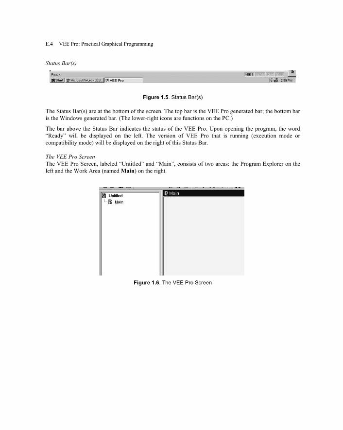
E.4 VEE Pro: Practical Graphical Programming
Status Bar(s)
Figure 1.5. Status Bar(s)
The Status Bar(s) are at the bottom of the screen. The top bar is the VEE Pro generated bar; the bottom bar
is the Windows generated bar. (The lower-right icons are functions on the PC.)
The bar above the Status Bar indicates the status of the VEE Pro. Upon opening the program, the word
“Ready” will be displayed on the left. The version of VEE Pro that is running (execution mode or
compatibility mode) will be displayed on the right of this Status Bar.
The VEE Pro Screen
The VEE Pro Screen, labeled “Untitled” and “Main”, consists of two areas: the Program Explorer on the
left and the Work Area (named Main) on the right.
Figure 1.6. The VEE Pro Screen

Appendix E: Introducing Objects, Icons, and Features E.5
Program Explorer
Figure 1.7. The Program Explorer
Program Explorer is accessed via the Menu Bar => View menu. If a check mark is displayed, the Program
Explorer area will appear on the left side of the screen. Eliminating the checkmark will cause the Program-
Explorer area to hide (go into the background). This is a toggle operation. The Program Explorer is a
graphical and hierarchical diagram of the program being examined.
Work Area
Figure 1.8. The Work Area
This is the area (Main) where programs are developed and displayed. It is located to the right of the
Program Explorer. Previously prepared programs can be displayed in this area so they can be run or
modified. In the upper-right corner, there are buttons that will minimize, maximize, or close the Work
Area.
In order to distinguish the Menu Bar from the Tool Bar, the notation: Menu Bar => is used. The Menu Bar
contains the titles: File, Edit, View, Debug, Flow, Device, I/O, Data, Display, Window, and Help.

E.6 VEE Pro: Practical Graphical Programming
Example: Select Menu Bar => Device => Virtual Source => Noise Generator indicates that Noise
Generator is the sub-sub-item within the sub-item Virtual Source within the item labeled Device on
the Menu Bar.
Note: Each object will appear initially as a blank rectangle that must be placed in the Work Area.
A single click will anchor and display that icon. Its default title and other properties can be
accessed by double-clicking on its top horizontal bar, which is a shortcut to the Properties box.
Menu Bar => Display
Figure 1.9. The Menu Bar => Display
From the Menu Bar, click sequentially on the following items:

Appendix E: Introducing Objects, Icons, and Features E.7
Menu Bar => Display => Note Pad
Figure 1.10. The Menu Bar => Display => Note Pad
Once the Note Pad is anchored, you may click inside the white space (edit area”). You will see a cursor,
shown as a blinking I-bar. The Note Pad enables you to write notes that explain the program in its editing
(white) area the left object in Figure 1.10.
The Note Pad upper-left symbol (-) can be used to access additional features (Restore, Move, Size,
Minimize, Clone, Replace, Help, Properties, Description, Add Terminal, Delete Terminal, Insert File,
Clear All, and Cut) the center object. These features will be described where appropriate. The “dot”
symbol displayed in the upper right of this object reduces the Note Pad to its Iconic View – the right-hand
object in Figure 1.10.
Note 1: The object left (dash) symbol is the object menu; the object right (dot) symbol converts
the object to an icon. These symbols apply to all objects.
Note 2: The darkened features are the ones accessible in this situation.

E.8 VEE Pro: Practical Graphical Programming
Menu Bar => Display => Waveform (Time)
Figure 1.11. The Menu Bar => Display => Waveform (Time)
This object represents an oscilloscope; it displays magnitude (Mag) versus time (Time). The Waveform
(Time) input (Trace 1) is on the left side of its object. The Waveform (Time) features are selected by
clicking the upper left “–”. These features are: Restore, Move, Size, Minimize, Clone, Replace, Help,
Properties, Description, Add Terminal, Delete Terminal, Auto Scale, Zoom, Clear Control, Center
Markers, Add Right Scale, Plot, and Cut. “Mag” characteristics can be changed by clicking on “Mag”. The
name “Mag” can be changed; also, its scale range and other parameters can be changed to match the
application. The name, color, line type, and point type of “Trace1” can be changed by clicking on
“Trace1”. Also, additional traces can be added via the “Add Terminal => Data Input” that can be accessed
via the upper-left symbol. The name “Time” and its parameters can be changed by clicking on “Time”.
Note 1: Most terminals on an object will be explained by a tooltip banner (flag) that will appear if
the mouse is held over that terminal, but not clicked, for approximately two seconds. If a square is
displayed, it indicates that you can make a “wire” connection from that terminal to another
terminal. A double-click will remove the initiated connection.
Note 2: Experience will show you those terminals whose name you can modify by clicking on that
terminal.

Appendix E: Introducing Objects, Icons, and Features E.9
Menu Bar => Display => AlphaNumeric
Figure 1.12. The Menu Bar => Display => AlphaNumeric
This box receives input from its left side. The characteristics are set by clicking the upper-left (-) symbol.
Sizing of the area for data can be adjusted by clicking the lower right and moving the arrow. The upper
right square converts it to an Iconic View.
Menu Bar => Device
From the Menu Bar, click on each of the items below.

E.10 VEE Pro: Practical Graphical Programming
Menu Bar => Device => Virtual Source => Function Generator
Figure 1.13. The Menu Bar => Device => Virtual Source => Function Generator
The Function Generator is the first Virtual Source. Its features are selected by clicking the upper left “–”.
These features are: Restore, Move, Size, Minimize, Clone, Replace, Help, Properties, Description, Add
Terminal, Delete Terminal, and Cut. Generator parameters are altered within the Generator white (editing)
space. There are seven functions available within the Generator Function pull-down menu. There are three
Phase units available within the Phase pull-down menu. The Generator has an Output Terminal labeled
“Func” on the right side for connecting the Generator to other objects. Double-clicking on Func causes a
box labeled “Output Terminal Information” to appear. This box is valuable when troubleshooting after
running a program.
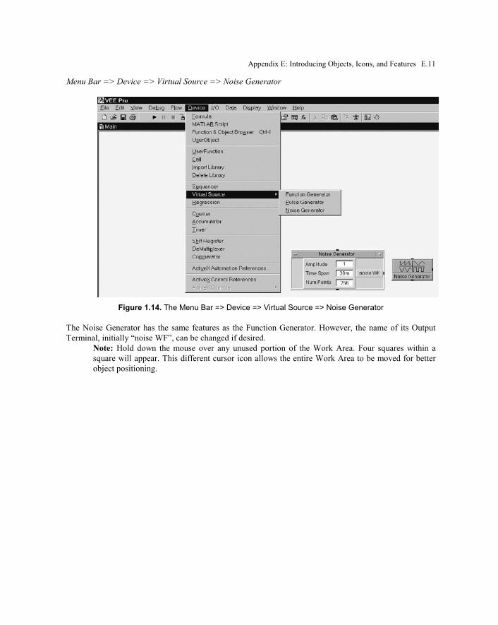
Appendix E: Introducing Objects, Icons, and Features E.11
Menu Bar => Device => Virtual Source => Noise Generator
Figure 1.14. The Menu Bar => Device => Virtual Source => Noise Generator
The Noise Generator has the same features as the Function Generator. However, the name of its Output
Terminal, initially “noise WF”, can be changed if desired.
Note: Hold down the mouse over any unused portion of the Work Area. Four squares within a
square will appear. This different cursor icon allows the entire Work Area to be moved for better
object positioning.

E.12 VEE Pro: Practical Graphical Programming
Menu Bar => Device => UserObject
Figure 1.15. Menu Bar => Device => UserObject
The UserObject initially appears as a closed object within Main. It is opened by double-clicking on its
Iconic View. The UserObject can contain one or more of interconnected objects that can be saved as a
library for future use. Its title can be changed by double-clicking on its top horizontal bar (below the Tool
Bar). Its Trig Mode can be changed; its Colors, and Fonts can be displayed.
The UserObject initially contains neither input nor output terminals. Examine the top three squares in the
UserObject upper-left corner:
• Click on the minimize (_) button; the UserObject Iconic View will appear just above the Status
Bar.
• Click on the overlapping double-square (maximize) button; the UserObject will shrink to a smaller
area within Main.
• Click on the X button; the Open View of the UserObject will disappear. You can bring it back by
double-clicking on the icon.
If the object totally disappears, then go to View => Program Explorer and toggle its title. Then double-
click on the UserObject title; its window will reappear in Main.
UserObject features are selected by clicking on the (-) symbol in its upper-left corner. These features are:
Restore, Move, Size, Minimize, Maximize, Cut, Copy, Clone, Help, Properties, Description, Add
Terminal, Delete Terminal, Make UserFunction, Unpack, Save Secured Version, Find, Print, Locate, Calls,
Create Panel, Delete Panel, and Close. The names for each added terminal may be changed by double-
clicking on that terminal.

Appendix E: Introducing Objects, Icons, and Features E.13
Menu Bar => Device => Formula
Figure 1.16. The Menu Bar => Device => Formula
The Formula Object initially appears with the default formula “2*A+3”. This formula can be modified as
desired. Its features are selected by clicking the upper left (-) symbol. These features are: Restore, Move,
Size, Minimize, Clone, Replace, Help, Properties, Description, Add Terminal, Delete Terminal, and Cut.
Terminals may be added or deleted. The input and output terminal default names can be changed by
double-clicking on the terminal. The name of the terminal corresponds directly to the variable name in the
Formula expression. The input terminal Required Type and Required Shape can also be changed by
double-clicking on the terminals.

E.14 VEE Pro: Practical Graphical Programming
Menu Bar => Device => Function & Object Browser
Figure 1.17. The Menu Bar => Device => Function & Object Browser Object
All of the operators available to help build formulas can be accessed via the Type window.
• When Operators is selected under Type, then Category and Operators windows appear.
• When a Function is selected under Type, then Category and Functions windows appear.
• Also, for the ActiveX objects, then Library, Class, and Members appear.
• When “VEE objects” is selected under Type, then Category and Members appear.
• When Instruments is selected under Type, then Instrument Category, Configured Instruments, and
Members appear.
There is a gray box across the bottom of Function & Object Browser. Further information regarding each
selected item will appear in this box.
Note: “A+B Adds two numbers” is shown above. When Create Formula is clicked, then the
Formula Object appears with A+B as its title. The title A+B remains displayed in the Iconic View.
Overall Reminders
Program Explorer
The Program Explorer is a Work Area that requires a significant amount of space on your screen. It is very
helpful whenever you want to examine how pieces of your program are connected. The Program Explorer
will automatically track your program structure and display it graphically in a hierarchical manner. Double-
clicking on a Program Explorer icon will immediately take you to that icon’s object. Also, you can provide
more room for your Main Work Area:
Appendix E: Introducing Objects, Icons, and Features E.15
Menu Bar => Select View => Program Explorer
There is a checkmark next to Program Explorer. Program Explorer can be toggled to select or deselect it.
Observe the effect on the screen display. Similarly, you can select and deselect the Tool Bar and the Status
Bar. Also, the width of the Program Explorer can be modified by holding the mouse over the right-hand
border of the Program Explorer window. It will change into a “splitter” cursor. Drag this cursor to change
the Program Explorer width.
Cloning Objects
Clicking on the upper left (-) symbol of an object will display a pull-down menu that includes Clone.
Cloning an object causes an exact duplicate of the original object. Its title and parameters can be changed
once it is placed in the Work Area. Cloning a given object may be repeated. Cloning large groups of
objects is not recommended. See the topic: UserFunctions.
Open View versus Iconic View
The Open View of an object displays all its available and controllable parameters and terminals. The
Iconic View provides only a visual description and the name of that object. However, all terminals are
accessible and can be connected. Closing an object requires clicking on its upper-right (•) symbol.
Opening an object requires double-clicking on any portion of that object. Program development is usually
performed in the Open View; programs are usually run in the Iconic View.
Program Development
Program Development is performed by connecting the appropriate objects in the Work Area. The
techniques and procedures are described in each lab. A cross-referenced index is given in Appendix B.
Run-Time Errors
After the program is developed, it is run. A VEE Run Time Error occurs when a program is prepared that
will not operate properly. Errors are noted after the Run arrow (sixth button from left on Tool Bar) is
clicked and an error box appears. The VEE Run Time Error box indicates the type of error and where it
occurred. That object will have a red border. The Go To button To indicates which object is at fault. The
Help button will provide a description of the error; it is not always helpful! The accessed Help dialog box
may be printed if desired. The last error can also be retrieved from the Menu Bar => View => Last Error
menu selection.
Note: Click on the black square in the Tool Bar to stop the program. Corrections to the program
may now be performed.

E.16 VEE Pro: Practical Graphical Programming
Lesson 2 Pre-lab
The VEE Pro Opening Development Screen
Figure 2.1. The VEE Pro Development Screen
Bitmap Transferring
Bitmaps in the form of pictures (art) may be converted from VEE Pro to other Windows applications, via
the clipboard. The applications must support Bitmap. Microsoft Word™ supports Bitmap. (The clipboard
cannot be viewed.) Its applications will be presented later. To copy an object: select one or more objects,
choose Copy from the Edit menu, switch to the other application, and choose Paste in the Edit menu.
Other ways to generate bitmaps from VEE Pro include the little savePanelImage (function) and the Web
Server capability. See the VEE Pro documentation for details.
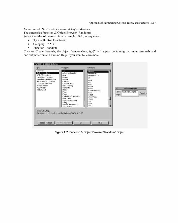
Appendix E: Introducing Objects, Icons, and Features E.17
Menu Bar => Device => Function & Object Browser
The categories Function & Object Browser (Random):
Select the titles of interest. As an example, click, in sequence:
• Type – Built-in Functions
• Category – <All>
• Function – random
Click on Create Formula; the object “random(low,high)” will appear containing two input terminals and
one output terminal. Examine Help if you want to learn more.
Figure 2.2. Function & Object Browser “Random” Object

E.18 VEE Pro: Practical Graphical Programming
Menu Bar => Data => Constant => UInt8
UInt8 is an object that provides a one-byte, unsigned (U) integer scalar – an absolute value without sign.
For this lesson, enter the desired integer (0 or 1) within the object white space (editing area).
Figure 2.3. Data => Constant => UInt8
The other constant integer objects are explained below.

Appendix E: Introducing Objects, Icons, and Features E.19
Object Title Bar
Any object title-bar name (which is in the center of the title bar) may be changed so its title is more
descriptive. Double-click on the object title bar; the object Properties box will appear with its existing title
highlighted. Type in the desired title; click OK.
Figure 2.4. Changing object title name
Main Title Bar; Enter Description
Click on the Main title bar with the right-hand mouse button; a pull-down menu will appear; select
“Description”; a dialog box – Description of “Main” – will appear. Enter the information that you wish to
appear in the documentation of that program.
Figure 2.5. Adding Main Title Bar description

E.20 VEE Pro: Practical Graphical Programming
Program Documentation
Select Menu Bar => File => Save Documentation. The “.vee” extension will change to a “.txt” extension
on the end of the program title. The program documentation is a description of the combined program
elements. VEE Pro steps through the program components and prints the properties of each object.
Figure 2.6. “Save Documentation File” window
Menu Bar => Data => Continuous => Real64 Slider (or Knob)
Select Menu Bar => Data => Continuous => Real64 Slider.
Figure 2.7. Real Slider Continuous-Data Object

Appendix E: Introducing Objects, Icons, and Features E.21
Select Menu Bar => Data => Continuous => Real64 Knob.
Figure 2.8. Knob Continuous-Data Object

E.22 VEE Pro: Practical Graphical Programming
Menu Bar => Data => Dialog Box => Int32 Input
Select Menu Bar => Data => Dialog Box => Int32 Input.
The Prompt/Label field typically contains “Enter Integer Value”; change this text if desired.
Enter a Default Value that is within the Value Constraint range; otherwise, an error message will appear.
The Error Message box constraints should agree with the Value Constraint numbers.
There are two types of dialog boxes: the Modal dialog box will cause a program “pause”. A UserObject or
UserFunction can be used to create a Non-Modal dialog box (with a panel) that will allow the program to
continue to run.
Figure 2.9. Data => Dialog Box => Int32 input and descriptors

Appendix E: Introducing Objects, Icons, and Features E.23
Menu Bar => I/O => To => File
Select Menu Bar => I/O => To => File.
Program results may be stored by using the ToFile Object; this object provides a location where the
program data (results) are stored. Input terminals can be added to send the specific data to a file;
transactions can be added by double-clicking the (<Double-click here>”. Data are taken from the input-
terminal pins (when they exist) and written to the specified file via transactions inside the object.
The data-location name “myFile” should be changed to be more specific so it will identify the stored data
location. When it is clicked, the query: “Write data into what file?” will appear.
• That file-location name may be chosen from the provided list; otherwise, a new file location may
be entered.
• If that file-location name already exists, then it will be highlighted when the “new” name is typed
into the editing area.
• If that new-location file name is to be added to the list, then click OK on the dialog box.
Figure 2.10. I/O => To => File Information (partial)

E.24 VEE Pro: Practical Graphical Programming
Figure 2.11. I/O => To => File Information (continued)
Figure 2.12. I/O => To => File Information (final)
Creating an Operator Interface
An Operator Interface can be created from an existing program. The Operator Interface allows any
operator to run a program without being able to change the connections and any other parameters that are
to be unavailable to the operator.

Appendix E: Introducing Objects, Icons, and Features E.25
The Operator Interface is created by first highlighting those objects (with the Ctrl key) to be included in
the operator’s Panel View. Then the mouse is placed on the Main menu white space and the mouse right-
hand button is depressed. “Add to Panel” is selected. An Operator Interface is then created. Only those
objects are displayed that can be modified; no connections are shown.
Figure 2.13. Panel View of an Operator Interface
In this example, the Function Generator is set to the Tri function which the operator can change. Once
“run” is depressed, the waveform will change from the displayed cosine to the newly selected Triangle
function.
Switching between the Detail View and the Panel View
The Main title bar will display two rectangles on its left-hand side. Touch the left rectangle to access the
Panel View; touch the right rectangle to access the Detail View. See Figure 2.14.
Figure 2.14. Switching between Detail View and Panel View
Changing colors and fonts on Panel
Return to Panel View. From the Object Menu, (the left object on the gray Panel View Title Bar), select
Properties, then Color. Click on the rectangular button to the right of “Background”. Select the color you
desire. See Figure 2.15.

E.26 VEE Pro: Practical Graphical Programming
Figure 2.15. Changing Panel-View colors
Changing colors and fonts on Objects
Double-click on a UserObject Title Bar; the Properties box will appear. Click on Colors; your choices will
include
• Panel View Background,
• Pop-Up Panel Title Background, and
• Pop-Up Panel Title Text.
This procedure is similar to “Changing colors and fonts on Panel” above. Color-coordination information
may be useful in visually “connecting” a variety of related objects.

Appendix E: Introducing Objects, Icons, and Features E.27
Menu Bar = > I/O => To => File
The ToFile Object provides access to storing program data. The data are accessed by double-clicking on
the ToFile “A” input terminal. See Figure 2.16.
Figure 2.16. Example of ToFile contents
Menu Bar = > I/O => From => File
Select Menu Bar = > I/O => From => File. The FromFile Object provides access to processed program
data. After the program is run, the data are accessed by double-clicking on the FromFile “X” output
terminal. See Figure 2.17.
Figure 2.17. Example of FromFile content

E.28 VEE Pro: Practical Graphical Programming
Alphanumeric Display Selection
The Alphanumeric Display Object can display text or numbers. The numbers must be in scalar (a data
shape that contains a single value), one-dimensional array, or two-dimensional array format. The
Alphanumeric Display Object will display only the last data sent via the input terminal.
A logging alphanumeric display will provide displays as text or numbers when a test is repeated more than
once – when data is sent to the object multiple times, such as in a loop. The logging alphanumeric input
data must be in scalar or in one-dimensional array shape.
Print Screen
Select Menu Bar => File => Print Screen. A dialog box will appear from which the selected printer and
number of copies can be selected. See Figure 2.18.
Note: VEE Pro will not allow a “Print Screen” if another Modal dialog box is already open.
Figure 2.18. The Print Screen Dialog Box
Deleting unneeded objects and connecting lines
Two types of scissors are available from the Menu Bar. See Figure 2.19. The left scissors are used to cut
unwanted objects whenever that object is highlighted. Any connecting lines are also deleted. The right
scissors are used to cut connecting lines between objects.
Figure 2.19. The Two VEE Pro Scissors

Appendix E: Introducing Objects, Icons, and Features E.29
Deleting unneeded terminals
Input and output terminals (pins) may be deleted. Click on an object upper-left (-) square. As an example,
select Delete Terminal; then select the type of (input) terminal you wish to delete. That terminal will be
automatically deleted, including its title. See Figure 2.20.
Note: A shortcut for deleting a terminal – hold the cursor over the terminal and depress Ctrl + D.
Figure 2.20. Deleting an Object terminal
Open or Save a File
As an example, select Menu Bar => File => Open. A File Directory dialog box (Open File) will appear
with a list of files that are available to be opened.
Note: It may be necessary to search the hierarchy of file folders to locate the desired file. This
approach is identical to that used in any PC-Windows application.
Save File works in a similar manner:
Menu Bar => File => Save
If a new name is to be given the file, then select:
Menu Bar => File => Save As….

E.30 VEE Pro: Practical Graphical Programming
Lesson 3 Pre-lab
Controlling and configuring instruments
There are many ways to control and configure instruments:
• Panel Drivers provide a simple user interface (or “front panel”) to control instruments from the
computer screen. Changing parameters in the VEE Pro panel driver Front Panel on the screen
changes the corresponding state of the physical instrument. Component drivers are a subset of
panel drivers.
• Direct I/O Object allows for transmitting of commands and reception of data over a variety of
supported interfaces.
• VXIplug&play drivers control instruments over VXI, GPIB, and other interfaces. The
VXIplug&play standard specifies how the drivers are written by the instrument vendor. Therefore,
their “look and feel” is similar.
For more information regarding controlling instruments, see the Lesson 4 Pre-lab below.
Menu Bar => I/O => Instrument Manager…
The Instrument Manager allows adding one or more instruments and devices to your VEE Pro program.
Properties of the instruments are set via the Properties button on the right side under “Instrument”. Click
“Add” under Instrument… . This displays the Device Configuration Dialog Box, which presents the
following fields. See Figure 3.1.
Figure 3.1. Instrument Manager Dialog Box with (Add) Instrument Properties
This configuration of instruments and settings is stored in a file (or can be saved within each .vee
program). My Configuration shows the path where the file is saved. Configurations for instruments can be
added for both real (physical) instruments and for instruments that you may not have connected live at this
time. The non-connected instruments can be configured as “NOT LIVE”. This allows you to create your
configuration and write your program. NOT LIVE instruments are usually given an address or zero.

Appendix E: Introducing Objects, Icons, and Features E.31
Under Instruments, Add…, four fields are given:
• Name (of instrument),
• Interface (to reach either the GPIB, Serial, GPIO, or VXI bus),
• Address (where 0 represents the address of an instrument not present (NOT LIVE) and 7xx
represents the address of the GPIB bus),
• Gateway: (“This host” is used to control instruments locally)
The Advanced Instrument Properties dialog box allows for the selection of Direct I/O, Plug&Play Driver,
and Panel Driver configurations.
Menu Bar => Flow => Start
The Start button activates the program. It is an alternative to the Run button when you are writing small
prototype programs. It is not recommended for large programs and runtime versions. The Start button can
only be moved by right-clicking on the Start-button Object.
Menu Bar => Flow => Do
The “Do” Object creates a branch point to control the flow of the execution of a thread.
Menu Bar => Flow => Repeat => For Count
For Count is an object that activates data being processed a specified number of times. The output of For
Count can be used as a value to activate succeeding objects. The three objects are shown in Figure 3.2.
Figure 3.2. Three ”Flow” objects
Menu Bar => Data => Collector
Collector is used to create a one-dimensional array from scalar input data. It can create an output array
from collected input arrays. When all data have been gathered, the XEQ pin informs the output that the
collected array of data is available. The Collector has two inputs: one for input (Data), the other is an
output trigger (XEQ).
Output Shape There are two selections. See Figure 3.3.
• 1 Dim Array - The output signal shape, regardless of the input signal, is a 1D Array.
• n+1 Dim Array - The input signals (arrays of n dimensions) are collected; the output is an array of
n+1 dimensions.
Figure 3.3. The Collector Object; both settings
Menu Bar => Device => Timer
An object whose output is the difference (in seconds) between its activation time (top-left pin) and its
completion time (bottom-left pin). The elapsed time is indicated in its display space. See Figure 3.4.

E.32 VEE Pro: Practical Graphical Programming
Figure 3.4. The Timer Object
Menu Bar => Device => UserObject
The UserObject initially appears as a closed Iconic View within Main or any other window. It is opened by
double-clicking on its icon. The UserObject can contain one or more interconnected objects that can be
saved as a library for future use. See Figure 3.5 for its three possible locations (views).
Figure 3.5. Three views of UserObject
Its title can be changed by double-clicking on its top horizontal bar (below the Tool Bar). Its Trig Mode,
can be changed; its Colors and Fonts can be displayed.
UserObject features are selected by clicking on the (-) symbol in its upper-left corner. These features are:
Restore, Move, Size, Minimize, Maximize, Cut, Copy, Clone, Help, Properties, Description, Add
Terminal, Delete Terminal, Make UserFunction, Unpack, Save Secured Version, Find, Print, Locate, Calls,
Create Panel, Delete Panel, and Close. The names for each added terminal may be changed by double-
clicking on that terminal.
Installing your own program within a UserObject is known as encapsulation. Installing one UserObject
within another is known as nesting. These are the building blocks of your more sophisticated programs; it
is known as achieving “top-down design” by programmers.
Rather than cloning a UserObject, it is preferable to apply a UserFunction that can be called and re-used in
multiple locations for any of your programs. The UserFunction is explained below.
Time 1
Time 2 T2 – T1

Appendix E: Introducing Objects, Icons, and Features E.33
Lesson 4 Pre-Lab
Additional information and updates are available via the Agilent Web site at
http://www.agilent.com/find/vee.
The telephone contacts for support are:
In the US, 800-452-4844.
In Canada, 877-894-4414
Outside the US and Canada, contact your country's Agilent support organization.
A list of contact information for other countries is available on the Agilent website:
http://www.agilent.com/find/assist
Download the Latest Version of the Agilent IO Libraries from:
http://www.agilent.com/find/iolib
“Hotfixes” must be obtained from Microsoft because Microsoft does not allow Agilent to distribute
Windows 2000 hotfixes.
Instrument Control Object
The VEE Pro User’s Guide section entitled: Easy Ways to Control Instruments contains extensive, detailed
descriptions regarding configuring and controlling instruments.
Instrument Control => Object Menu => Add Terminal => Control
The VEE Pro Object Control adds an asynchronous control input terminal to an object. Use Control Input
to add asynchronous inputs, such as Reset or Clear, to an object. After selecting Control Input, choose the
control to add information from a dialog box. See Figure 4.1.
Figure 4.1. Accessing the object control input terminal
Activation of a control input pin does not cause the object to operate; it only forces a particular action to
happen, such as Clear.

E.34 VEE Pro: Practical Graphical Programming
Instrument I/O Data Types
VEE Pro provides many data types used for instrument I/O. It manipulates and stores all integer values as
Int32 data types and all real numbers as Real64 data types. However, instruments generally support 16-bit
integers or 8-bit bytes; some instruments support 32-bit real data. VEE Pro provides the following data
types for general programming in the Menu Bar => Data => Constant and Instrument Manager “instrument
I/O”. See Table 4.1.
Table 4.1. VEE Pro Instrument Data Types
VEE Data Type Constant Description
Byte An 8-bit two’s complement byte (-128 to +127). Byte is used to READ BINARY,
WRITE BINARY, and WRITE BYTE instrument I/O instructions only. UInt8 is
the default data type.
Int16 A 16-bit two’s complement integer (-32768 to +32767).
Int32 A constant 32-bit integer scalar or ID Array. As an example: Use Int32 to set an
integer constant or to get a user input. If Global Format is off, specify the number
format for integer numbers to be displayed on this object. The choices are Decimal
(e.g. 42), Octal (e.g. #Q52), Hexadecimal (e.g. #H2a), and Binary (e.g.
#B00101010). Default is Decimal. The Default Value input allows a change in the
current value(s). This input requires an integer value, either a Scalar or an Array
1D. The Constant is reconfigured to match the shape of the incoming data. The
Initial Value field is a scalar, even if Int32 is configured to be an array.
Real32 A 32-bit real number that conforms to the IEEE 754 standard: (+/-3.40282347
E+/-38)
Real64 A 64-bit real number. The Global Format specifies the number format for real
numbers to be displayed. Typical choices are Fixed (98.6000), Scientific
(9.8600E+01), Engineering (98.6000E0), Standard (98.6), and Time Stamp (Wed
01/Jan/2003 17:01:38). Default is Standard.
UInt8 A constant 1-byte unsigned integer, scalar or 1D array. As an example: Use UInt8
as a prompt on a panel view, change the name of the UInt8 Object to a prompt
such as “Enter the number of seconds to delay:”. If Global Format is off, specify
the number format for integer numbers to be displayed. The choices are Decimal
(42), Octal (#Q52), Hexadecimal (#H2a), and Binary (#B00101010). Default is
Decimal. The Initial Value field is always a scalar, even if UInt8 is configured to
be an array.
Notes for Table 4.1:
Int32:
Wait for Input – When the check box is selected, the object does not operate until the object's
value is changed. Thus, the constant acts like a “Confirm” button. When the check box is not
selected, the object operates as soon as any constraints are met, and the currently selected value is
the output. Default is off.
Auto Execute – When the check box is selected, the object operates and starts the rest of the
program when a value is selected. Thus, the constant acts like a “Start” button. If the program is
already running, Auto Execute is ignored. Default is off. Auto Execute is not recommended for
large programs.

Appendix E: Introducing Objects, Icons, and Features E.35
UInt8:
Initialize is most often used for initializing values inside a UserObject or UserFunction. The other
method for setting initial values is the Default Value control pin available on most data constants.
The Default Value input allows you to change the current value(s). This input requires an integer
value, either a Scalar or an Array 1D. The Constant is reconfigured to match the shape of the
incoming data.
Common Instrument Data Type Characteristics
The following Menu Bar => Data => Constant objects have common characteristics, including: Number
Format, Default Value Control Input, Wait for Input, Auto Execute, and Initialize at Prerun & Activate.
Data constants only support scalar and 1D arrays. VEE Pro usually supports arrays up to ten dimensions.
Use Alloc Array or Formula [I.a.b] type of syntax to create larger dimensional arrays that are greater than
ten dimensions.
Note: Instruments may require ASCII, binary Real32, and binary Int32. Binary will run programs
much faster than ASCII. VXIplug&play requires memory allocation for direct I/O; there is a
tab on each plug&play driver panel to allocate memory.
Installing Hardware
Consult the Agilent Web site to determine the latest information regarding level of Windows software
support for your hardware installation. Also, before you install your IO Libraries software, you should
install any new hardware in your computer. After the hardware is installed, turn the computer on and allow
it to boot. If you are adding plug&play hardware, when you log on, Windows may display a Wizard to
guide you through the process of installing drivers for new hardware. Hardware examples include:
82350 PCI GPIB card
The 82350A card is self-configuring. It will “Plug & Play”. After installing this card into the PCI
or ISA slot, the I/O libraries are then installed. “Automatically Configure” is selected following
software installation.
E8491 VXI interface
If you install a 1394 OHCI card and want to configure an E8491, you should install the 1394 card
in the computer, connect the 1394 cable between the card and the E8491 and power up the VXI
card cage before booting the computer. Below are the configuration notes. For information on
Windows XP, consult the Agilent Web site.
Configuration notes:
1. If, on Windows 98 or Window 2000, you attempt to configure an E8491 card but none were
found on your system, verify that all your VXI mainframes are powered on and that your
1394 cables are connected before running IO Config. If you are still having trouble, refer to
the E8491 Troubleshooting Guide.
2. Windows 2000 support for the following interfaces has been added: E8491 IEEE 1394 to
VXI interface 82341C and 82350 GPIB Cards.
3. Fixes: In certain topologies, the E8491 hardware is not properly identified on the 1394 bus.
This will result in inconsistent behavior when the VXI resource manager tries to configure
instruments in the VXI card cages. Behavior may include timeout errors while attempting to
communicate with a particular instrument, and/or instruments appearing in cages where they
are not actually located. Try reversing the cable connections to the ports on the host interface

E.36 VEE Pro: Practical Graphical Programming
card. In general, cable connections with longer chains of E8491’s should be on lower host
ports. Don't re-run setup too quickly. After the IO Libraries Setup program exits, it takes
several seconds to clean up and unload itself from memory. If Setup is re-run before this
process is complete, you may see an error message or find that the re-installation does not
behave as expected.
Windows 2000
OHCI Card Driver: If the 'Found New Hardware Wizard' appears and prompts you to install the
driver for a 'Texas Instruments OHCI Compliant IEEE 1394 Host Controller', you will need to get
and install the drivers for this card from the Windows 2000 CD that came with your computer.
These drivers may already be installed and in that case, the 'Found New Hardware Wizard' for this
device will not appear. E8491 Driver: If the 'Found New Hardware Wizard' appears and prompts
you to install the driver for a 'Hewlett-Packard HP8491A', you can find the driver for this device
(1394ipt.inf) in the 'Windows 2000' subdirectory of the Agilent IO Libraries CD.
Windows NT 4.0
Because Windows NT is not a Plug&Play OS, all necessary driver installation and configuration
is performed when you install the IO Libraries.
Windows 98
OHCI Card Driver: If the 'Add New Hardware Wizard' appears and prompts you to install the
driver for a 'Texas Instruments OHCI Compliant IEEE 1394 Host Controller', you will need to get
and install the drivers for this card from the Windows 98 CD that came with your computer.
E8491 Driver: If the 'Add New Hardware Wizard' appears and prompts you to install the driver
for a 'Hewlett-Packard HP8491A', you can find the driver for this device (1394ipt.inf) in the
'Windows 2000' subdirectory of the Agilent IO Libraries CD.
82335B Card
This real-instrument interface card is difficult to configure. If this card must be used, install the
card “as is” and then contact Agilent technical support for real-time troubleshooting assistance.
82341D Card
This real-instrument interface card is self-configuring. It will “Plug & Play”. After installing this
card into the PCI or ISA slot, the I/O libraries are then installed. “Automatically Configure” is
selected following software installation.
Note: Some personal computers have 32-bit EISA backplanes. If you installed an Agilent 82340 or
82341 GPIB interface in an EISA slot, you may wish to run the EISA configuration utility
provided with your computer. The EISA configuration utility will assign hardware resources to
the interface to avoid system conflicts. When you ran the Agilent IO Libraries installation Setup
program, the EISA .CFG files were placed in the EISACFG directory under the SICL base
directory (for example, under C:\SICL95\EISACFG or C:\SICLNT\EISACFG if you installed the
SICL software in the default location). When you run the EISA configuration utility and assign
resources, be sure to use the same settings as used with the Agilent IO Libraries configuration
utility (IO Config).
RS 232 Serial Ports: The following are formatted for RS-232 Serial Ports:
E2050 LAN to GPIB
E2070 GPIO Cards
SICL and VISA LAN Client
SICL LAN Server
E8491 Support on Windows 98 has been added.

Appendix E: Introducing Objects, Icons, and Features E.37
Installing IO Libraries and Configuring Interfaces
Refer to Table 4.2 and “Agilent IO Libraries Installation and Configuration Guide for Windows”. Also,
refer to the Agilent web page for the latest installation information.
Table 4.2. Agilent IO Library Versions
Version Installed Action First See “Getting Started”
None Install a new version of the Agilent IO
library
Installing new IO libraries
H.01.03 or earlier Upgrade existing IO libraries to the
latest version
Upgrading existing IO libraries
J.01.00 or later Modify, repair, or remove the same
version of the existing IO libraries
Maintaining existing IO libraries
After installing any hardware and drivers needed for IO, you should then install the Agilent IO Libraries by
running 'Setup' from the Agilent IO Libraries CD. Before an interface can be used with SICL or Agilent
VISA, IO Libraries must configure the interface. This is normally done automatically during the
installation or it can be done manually using the 'IO Config' utility located in the 'Agilent IO Libraries'
program folder.
The I/O Configuration program contains the following 'Options' selections in its menu:
VISA Logging
Off (Default)
Message Viewer: Log to the Message Viewer application if available.
Event Viewer: Debug Window Log using Windows OutputDebugString(). (This is useful in
debuggers.)
SICL Yield (Windows 98)
False (Default): SICL does not yield the CPU during I/O.
SICL Yield must be 'False' for proper operation of some VXIplug&play drivers. This will
prevent a potential deadlock from within a Windows message handler.
True: SICL yields the CPU during I/O.
The following I/O interfaces are supported for 32-bit applications; 16-bit applications are not supported:
Agilent E8491 IEEE 1394 ("Fire Wire") to VXI Interface
SICL and VISA
Agilent E985x VXI Pentium (R) Controller (VXI and GPIB)
SICL and VISA
Agilent E623x VXI Pentium (R) Controller (VXI and GPIB)
SICL and VISA
Agilent 82340 GPIB Card (ISA) &
Agilent 82341A GPIB Card (ISA) &
Agilent 82341B GPIB Card (ISA) &
Agilent 82341C GPIB Card (ISA) &
Agilent 82350 GPIB Card (PCI)
SICL and VISA
For Agilent USB to GPIB interface cards, see www.agilent.com
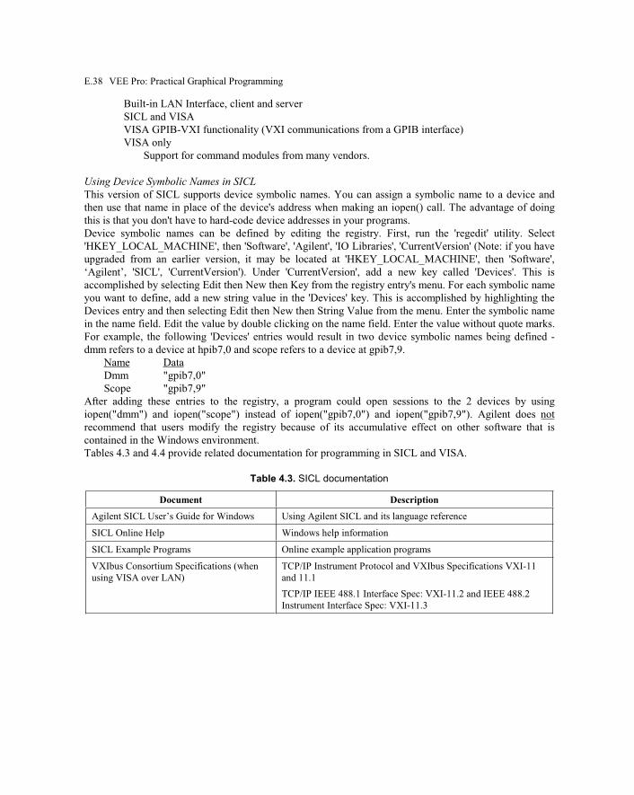
E.38 VEE Pro: Practical Graphical Programming
Built-in LAN Interface, client and server
SICL and VISA
VISA GPIB-VXI functionality (VXI communications from a GPIB interface)
VISA only
Support for command modules from many vendors.
Using Device Symbolic Names in SICL
This version of SICL supports device symbolic names. You can assign a symbolic name to a device and
then use that name in place of the device's address when making an iopen() call. The advantage of doing
this is that you don't have to hard-code device addresses in your programs.
Device symbolic names can be defined by editing the registry. First, run the 'regedit' utility. Select
'HKEY_LOCAL_MACHINE', then 'Software', 'Agilent', 'IO Libraries', 'CurrentVersion' (Note: if you have
upgraded from an earlier version, it may be located at 'HKEY_LOCAL_MACHINE', then 'Software',
‘Agilent’, 'SICL', 'CurrentVersion'). Under 'CurrentVersion', add a new key called 'Devices'. This is
accomplished by selecting Edit then New then Key from the registry entry's menu. For each symbolic name
you want to define, add a new string value in the 'Devices' key. This is accomplished by highlighting the
Devices entry and then selecting Edit then New then String Value from the menu. Enter the symbolic name
in the name field. Edit the value by double clicking on the name field. Enter the value without quote marks.
For example, the following 'Devices' entries would result in two device symbolic names being defined -
dmm refers to a device at hpib7,0 and scope refers to a device at gpib7,9.
Name Data
Dmm "gpib7,0"
Scope "gpib7,9"
After adding these entries to the registry, a program could open sessions to the 2 devices by using
iopen("dmm") and iopen("scope") instead of iopen("gpib7,0") and iopen("gpib7,9"). Agilent does not
recommend that users modify the registry because of its accumulative effect on other software that is
contained in the Windows environment.
Tables 4.3 and 4.4 provide related documentation for programming in SICL and VISA.
Table 4.3. SICL documentation
Document Description
Agilent SICL User’s Guide for Windows Using Agilent SICL and its language reference
SICL Online Help Windows help information
SICL Example Programs Online example application programs
VXIbus Consortium Specifications (when
using VISA over LAN)
TCP/IP Instrument Protocol and VXIbus Specifications VXI-11
and 11.1
TCP/IP IEEE 488.1 Interface Spec: VXI-11.2 and IEEE 488.2
Instrument Interface Spec: VXI-11.3

Appendix E: Introducing Objects, Icons, and Features E.39
Table 4.4. VISA Documentation
Document Description
Agilent VISA User’s Guide Using Agilent VISA and its language reference
VISA Online Help Windows help information
VISA Example Programs Online example application programs
VXI Plug&Play System Alliance VISA
Library Specification 4.3
Specifications for VISA
IEEE Standard Codes, Formats, Protocols,
and Common Commands
ANSI/IEEE Standard 488.2-1992
VXIbus Consortium Specifications (when
using VISA over LAN)
TCP/IP Instrument Protocol and VXIbus Specifications VXI-11
and 11.1
TCP/IP IEEE 488.1 Interface Spec: VXI-11.2 and IEEE 488.2
Instrument Interface Spec: VXI-11.3
Additional Visual BASIC Programming Notes
You can now pass any data type instead of just strings. This allows you to read and write binary data with
Visual BASIC for the following commands: iread, Ifread, Iwrite, Ifwrite, iswap, ileswap, and ibeswap.
The isetbuf function is now supported with Visual BASIC.
The igetlulist function is not implemented. It currently returns to Visual BASIC with error
I_ERR_NOTIMPL.
The igetaddr function is not implemented. It currently returns to Visual BASIC with error
I_ERR_NOTIMPL.
The ivxirminfo function does not correctly return the last two arrays in the structure (int_handler() and
interrupter() ). All other fields are correctly returned.
The igetluinfo function does not correctly return the hwargs() array. All other fields are correctly returned.
Sample files and a vbreadme.txt file documenting VISA calls from Visual BASIC 4.0 have been included
in the following directory (assuming you have installed in the standard location) for Windows NT:
c:\vxipnp\winnt\hpvisa\samples\vb
For all other versions, consult the Agilent Web site.
Warnings
LAN
The LAN server on Windows NT does not start automatically after a reboot as the manual says.
You need to either start it manually by double clicking its icon in the HP I/O Libraries folder, or
you can create a shortcut to it in your StartUp folder.
VISA viLock()/viUnlock() does not work on devices accessed via LAN. This implementation
supports the TCP/IP Instrument Protocol but it is known to differ from the specifications in the
following ways:

E.40 VEE Pro: Practical Graphical Programming
The device_abort RPC is not supported.
Rules B.4.17 and B.4.18 of VXI-11.1 are not supported by the current implementation. As noted
in observation B.5.1 of VXI-11.1, changes are anticipated to VXI-5. Due to these possible
changes and the fact that the current revision of VXI-5 does not require that any particular VXI-5
commands be implemented, the current LAN server implementation does not support VXI-5
operations.
Fast Data Channel (FDC)
This version of VISA uses a separate DLL to support the FDC protocol. This DLL is not supplied
by Agilent Technologies. Contact the supplier of your FDC capable hardware for information on
how to obtain and install the FDC DLL. If you attempt to set FDC-related attributes and the FDC
DLL has not been installed, you will receive a VI_ERROR_NSUP_ATTR error.
I-SCPI
I-SCPI was implemented ONLY for BACKWARD COMPATIBILITY and migration purposes. It
should not be used for new designs. Additional I-SCPI information is available the file:
c:\vxipnp\winnt\bin\iscpinfo.txt (Windows NT)
or
c:\vxipnp\win95\bin\iscpinfo.txt (Windows 95 and Windows 98)
Beginning with version G.02.00 of the I/O Libraries, the 32 bit I-SCPI drivers have changed from
a SICL to a VISA based implementation. This change should be invisible to you. Programs which
use I-SCPI should continue to function without modification unless a VISA based I-SCPI driver is
not available for an instrument you are using. There will be no new development on the SICL
based I-SCPI drivers.
Note that even though the I-SCPI drivers in this implementation are VISA based, I-SCPI may
only be used with SICL programs. VISA programs cannot use I-SCPI.
The Agilent E8491 IEEE-1394 to VXI product will only work with the VISA based I-SCPI
drivers.
Currently VISA based I-SCPI drivers are not available for the DDCC-1553 and E1450. If you are
using I-SCPI with these devices, you will need to use the SICL based I-SCPI drivers which are
not available on this release of the I/O Libraries. If you need to use the SICL based I-SCPI
drivers, do not upgrade to this version of the I/O Libraries. Version G.02.02 was the last version
of the Agilent I/O Libraries to contain support for SICL based I-SCPI.
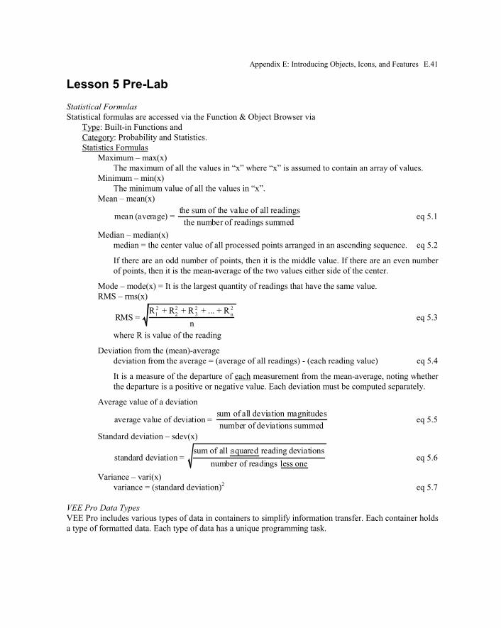
Appendix E: Introducing Objects, Icons, and Features E.41
Lesson 5 Pre-Lab
Statistical Formulas
Statistical formulas are accessed via the Function & Object Browser via
Type: Built-in Functions and
Category: Probability and Statistics.
Statistics Formulas
Maximum – max(x)
The maximum of all the values in “x” where “x” is assumed to contain an array of values.
Minimum – min(x)
The minimum value of all the values in “x”.
Mean – mean(x)
mean (average) = the sum of the value of all readings
the number of readings summed eq 5.1
Median – median(x)
median = the center value of all processed points arranged in an ascending sequence. eq 5.2
If there are an odd number of points, then it is the middle value. If there are an even number
of points, then it is the mean-average of the two values either side of the center.
Mode – mode(x) = It is the largest quantity of readings that have the same value.
RMS – rms(x)
RMS = R
1
2 + R2
2 + R3
2 + ... + Rn
2
n eq 5.3
where R is value of the reading
Deviation from the (mean)-average
deviation from the average = (average of all readings) - (each reading value) eq 5.4
It is a measure of the departure of each measurement from the mean-average, noting whether
the departure is a positive or negative value. Each deviation must be computed separately.
Average value of a deviation
average value of deviation = sum of all deviation magnitudes
number of deviations summed eq 5.5
Standard deviation – sdev(x)
standard deviation = sum of all squared reading deviations
number of readings less one eq 5.6
Variance – vari(x)
variance = (standard deviation)2 eq 5.7
VEE Pro Data Types
VEE Pro includes various types of data in containers to simplify information transfer. Each container holds
a type of formatted data. Each type of data has a unique programming task.

E.42 VEE Pro: Practical Graphical Programming
The data shape is either a scalar or an array. A scalar is a single alphanumeric value; an array is a
collection of identical data types.

Appendix E: Introducing Objects, Icons, and Features E.43
VEE Pro provides 14 data types that can perform a wide variety of functions; See Table 5.1.
Table 5.1. VEE Pro data types
Data Type Description
UInt8 UInt8 is an 8-bit two's complement unsigned integer (0 to 255).
Int16 Int16 is a 16-bit two's complement integer (-32768 to 32767).
Int32 A 32-bit two’s complement integer (-2147483648 to 2147483647); a whole number whose decimal
equivalent has no decimal portion, such as either 1 or 321.
Real32 A 32-bit real that conforms to the IEEE 754 standard (±3.40282347E±38).
Real64 A 64-bit real that conforms to the IEEE 754 standard; its decimal equivalent (+/- 1.797693138623157
E308) has a decimal portion, such as 3.2, 12.56.
PComplex A Polar Complex magnitude and phase component in the form (mag. @phase). Phase is set by default
to degrees, but can be set to radians or gradians with the File => Default Preferences => Trig Mode
setting.
Complex A rectangular or Cartesian complex number having a real and imaginary component in the form (real,
imag). Each component is Real. For example, the complex number 1 + 2i is represented by (1,2).
Waveform A composite data type of time domain values that contains the Real values of evenly-spaced, linear
points and the total time span of the waveform assumed to start at time zero. The data shape of a
Waveform must be a one-dimensional array.
Spectrum A composite data type of frequency domain values that contains the PComplex values of points and the
frequency start and stop times.
Coord A composite data type that contains at least two components in the form (x,y,…). Each component is
Real64. The data shape must be a Scalar or a 1D Array.
Enum A group of text strings; each has an associated integer value; the Unum has only one current value.
You can access the integer value with the ordinal (x) function.
Text A string of alphanumeric characters, such as abc123, gef, or 798.
Record A composite data type with a field for each type. Each field has a name and a container, which can be
of any type and shape (including Record).
Object Used for ActiveX Automation and Controls, a reference to an ActiveX control or a reference returned
if from an Automation call. Can also refer to a named VEE object and “get” and “set” properties via
the program.
VEE Pro Analysis Capabilities
The math functions are given in the Menu Bar => Device => Function & Object Browser menu: choices
for Built-in Functions and Operators. To create your own math functions, you can
• create the function with the Formula Object
• write the function in a compiled language such as C and link it to VEE Pro
• communicate with another software application from VEE, such as MATLAB®
Multiline Formula Techniques
Multiline formulas can be entered into the Formula Object editing area (white space). When explanatory
text is desired, then each line of explanatory text must be preceded by two forward slashes (//). The actual
instructions are separated with a semicolon (;). See Figure 5.1.

E.44 VEE Pro: Practical Graphical Programming
Figure 5.1. A Formula Object containing text and instructions
Operators
Each Operator is accessed via Function & Object Browser. See the Help menus and Appendix C.
Arithmetic: +, -, *, /, ^, DIV, MOD
Assignment: objectvalue=1, a[2]=b, a[2,*,5:6,4]=b, rec.field=b, rec.field[2]=b, rec[2].field=b,
globalA=2*b+3, tmp=a, a=b, b=tmp; tmp=a[2], a[2]=a[3], a[3]=tmp
Comparison: ==, ~=, !=, <=, >=, <, >
Logical: AND, OR, XOR, NOT
Miscellaneous: object.value, [1,2,3], [a,b,c], a[2], a[5,3:4,*], rec.field, PI, TRUE, FALSE, (a?b:c)
Built-in Functions
The Function & Object Browser built-in function details are given in their related Help menus and
Appendix C. The specific built-in functions are:
ActiveX Automation Power (Functions)
Array Probability & Statistics
Bessel Real Parts
Bitwise Signal Processing
Calculus String
Complex Parts System Information
Data Filtering Time & Date
Generate Trig (Functions)
Matrix Type Conversion
Panel
Note: All the above functions can be nested.
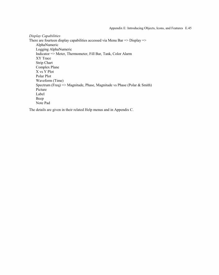
Appendix E: Introducing Objects, Icons, and Features E.45
Display Capabilities
There are fourteen display capabilities accessed via Menu Bar => Display =>
AlphaNumeric
Logging AlphaNumeric
Indicator => Meter, Thermometer, Fill Bar, Tank, Color Alarm
XY Trace
Strip Chart
Complex Plane
X vs Y Plot
Polar Plot
Waveform (Time)
Spectrum (Freq) => Magnitude, Phase, Magnitude vs Phase (Polar & Smith)
Picture
Label
Beep
Note Pad
The details are given in their related Help menus and in Appendix C.

E.46 VEE Pro: Practical Graphical Programming
Lesson 6 Pre-Lab
There are four specific operations that will be either discussed or referenced in Lesson 6:
• using the Collector and Concatenator objects
• using the To/From File objects for I/O Transactions
• sending a Real Array to a File
• retrieving data using the FromFile Object
Menu Bar => Data => Collector
The collector is an object that can collect data from multiple iterations from a loop and generate a single
array of data. It can accept multiple types of data, but only one type of data will be the output. The first
piece of data determines the output type; if other input data in the loop is another type, then it is converted
to the first output type. The collector can take a stream of scalar values in a loop and concatenate them to
form an array.
Menu Bar => Data => Concatenator
The Concatenator can also be used. It gathers elements from multiple sources and combines them into a
data container. The Concatenator, or its formula expression concat ( ), allows you to join elements from
several inputs. When all inputs to a Concatenator have data, then the Concatenator combines these inputs
together into a single data container. It then offers these data points as a one-dimension array.
Note: The Collector is preferred when you are gathering data in a loop – each iteration of the loop
generates a piece of scalar or array data and you want to gather all the data from each loop
iteration. You may then use the data at the end of the loop. The Concatenator is preferred when you
have multiple pieces of data and want to join them together.
To/From Files
The ToFile and FromFile objects were first used in Lesson 2. They are examined in greater detail below.
There are some basic concepts that you should understand about these objects.
• A data file is opened on the first READ or WRITE transaction. When the program ends, VEE Pro
closes any open files automatically.
• VEE Pro maintains one read pointer and one write pointer per file regardless of how many objects
are accessing the file. The read pointer identifies the next data item to be read and the write pointer
indicates where the next data item is to be written.
• You can append data to an existing file or overwrite previous data.
If the Clear File at PreRun setting is checked in the Open View of the ToFile Object, the write pointer
starts at the beginning of the file.

Appendix E: Introducing Objects, Icons, and Features E.47
If the Clear File at PreRun setting is unchecked, the write pointer is positioned at the end of the existing
file.
• Each WRITE transaction appends information to the file at the location of the write pointer. If an
EXECUTE CLEAR transaction is performed, the write pointer moves to the beginning of the file
and erases the file contents.
• A read pointer starts at the beginning of a file and advances through the data depending upon the
READ transactions. You may perform an EXECUTE REWIND in the FromFile Object to move
the pointer back to the beginning of the file without erasing the file contents.
To use FromFile, you need to know the format and location of the stored data.
Introduction to Understanding I/O Transactions
I/O Transactions are used to communicate with instruments, files, strings, the operating system, interfaces,
other programs, and printers. The example of Figure 6.1 shows a ToFile Object sending (writing) the data
of variable “a” on input pin a to a file named myFile. The highlighted line is known as a transaction line. It
contains the default transaction statement: WRITE TEXT a EOL. When you double-click it, an I/O
Transaction dialog box appears (Figure 6.1) which configures your specific transaction statement. You can
add inputs to accept data from your program.
Note: If a Direct I/O channel address is active, then a real instrument must be connected to it.
Figure 6.1. The ToFile Object with its I/O Transaction Dialog Box
Different objects call different forms of this dialog box which share certain common elements. We want to
stress: the “actions”, the “encodings”, the “expression list”, the “format”, and the “end-of-line” (EOL)
sequence. These elements form the structure for writing data, which usually takes the following format:
<action><encoding><expression list><format><EOL>
It is important for you to know that the <action>, <encoding>, and <format> elements provide selection
via their individual drop-down menus. The <EOL> button toggles the End-of-Line character ON and OFF.
Only the <expression list> field requires keyboard entry.

E.48 VEE Pro: Practical Graphical Programming
The tables and comments that follow will provide you a basic understanding of these elements and the
actions they perform. The most common actions available are READ, WRITE, EXECUTE, and WAIT.
See Table 6.1.
Table 6.1. Actions and their explanations
Action Explanation
READ Reads data from the specified source using its encoding and format.
WRITE Writes data to the specified target using its encoding and format.
EXECUTE Executes a specific command. For example, EXECUTE REWIND repositions a file’s read or
write pointer to the beginning of the file without erasing the contents. .EXECUTE CLOSE
closes an open file.
WAIT Waits the specified number of seconds before the next transaction.
Note: You can also examine a number of actions for Menu Bar =>
I/O => Advanced I/O Operations by exploring objects in that menu.
Encoding and formats refer to the way data are packaged and sent. For instance, a TEXT encoding sends
data in the form of ASCII characters. The TEXT encoding could be formatted in several ways. Suppose,
for example, you want to send a string of numbers and letters to a file. A WRITE TEXT STRING
transaction would send the entire string – represented as ASCII characters. On the other hand, a WRITE
TEXT REAL transaction would extract only the real numbers from the string of numbers and letters, and
send those using ASCII characters for the individual digits. Table 6.2 provides explanations of encodings:
Table 6.2. Encoding explanations
Encoding Explanations
TEXT Reads or writes all data types in a human-readable form (ASCII) that can be edited or ported
easily to other software applications. VEE Pro numeric data is automatically converted into
text.
BYTE Converts numeric data to binary integers. Sends/receives the least significant byte.
CASE Maps an enumerated value or an integer to a string and reads or writes that string. For
example, you could use CASE to accept error numbers and write error messages.
BINARY Handles all data types in a machine-specific binary format.
BINBLOCK Uses IEEE488.2 definite-length block headers with all VEE Pro data types in binary files.
CONTAINER Uses VEE Pro-specific text format with all data types.
CONTAINER Uses VEE Pro specific text format with all data types.
In a write transaction, an “expression list” is simply a comma-separated list of expressions that will be
evaluated to yield the data sent. The expression may consist of a mathematical expression, an input pin
name, a string constant, a VEE Pro function, a UserFunction or a Global Variable, or any combination of
them. The expression is very similar to a formula; however, the assignment of “a=b*3” syntax is not
allowed. In a read transaction, the “expression list” should consist of a comma-separated list of output-
terminal names indicating where the data to be read in should be placed.

Appendix E: Introducing Objects, Icons, and Features E.49
Data types and formats were presented in Lesson 3, including reading data from instruments. Most of those
formats apply to I/O transactions.
The EOL (end-of-line sequence of characters) may be turned on or off. You can specify the EOL sequence
by opening the object menu of most of the “To” objects under Menu Bar => I/O => To => objects and
selecting Properties…. Then select Data Format and make your changes under Separator Sequence.
The details of these operations are given below along with introductions to arrays and the To/From Files.
Introduction to Arrays
An array is a collection of like data types such as integer, real, and text. Arrays store multiple values of
data, storing each data value in a contiguous memory location. This allows VEE Pro to accommodate
programs performing repetitive computations.
An M-by-N array consists of M rows and N columns. Each row and each column illustrates an array
dimension; in a 2-by-2 array the number of elements in each row determines the number of columns in the
array. In theory, an array can contain an unlimited number of dimensions. See Figure 6.2 which is an
example of a 3 row, 3 column array.
Col 0 Col 1 Col 2
[0, 0] [0, 1] [0, 2] Row 0 ( 0) (1) (2)
[1, 0] [1, 1] [1, 2] Row 1 (3) (4) (5)
[2, 0] [2, 1] [2, 2] Row 2 (6) (7) (8)
1st row 3rd element
2nd row 6th element,
3rd row 9th (n-1) element
Figure 6.2. A Three-Row, Three-Column Array
In practice, three-dimension arrays (rather than four-dimension arrays) are used because they are easy to
visualize and process. Arrays whose dimensions are four, five, and beyond are devised and applied
primarily by mathematicians.

E.50 VEE Pro: Practical Graphical Programming
Indexing for arrays is zero-based; that is, the first element is numbered zero, the second element is
numbered one, and the nth element numbered n - 1. Brackets [ ] are used to indicate the position of each
array element.
Example: If the array A holds the elements [4, 5, 6], then A[0] = 4, A[1] = 5, and A[2] = 6.
The brackets either state the position of an array element or declare the value stored in the array. The
syntax <arrayName>[index] is used to refer to that element in an array, known as the subarray syntax. The
[<value>,<value>, … ] syntax is used to create an array from the given values.
A one-row, three-column, one-dimension array is shown in Figure 6.3; the method of addressing is the
same as for a multi-row array.
[0] [1] [2]
(0) (1) (2)Row 0
Figure 6.3. A one-row, three-column, one-dimension array
Accessing arrays requires the following notation:
The colon “:” is used to indicate a range of elements.
Example: A[0:2] = [4, 5, 6] where 0, 1, 2 are the data addresses or indices and 4, 5, 6 are their
data values (in the same order).
The asterisk “*” is a wild card used to specify all elements in a particular array dimension.
Example: A[*] will access all elements of array A for further processing.
In the subarray syntax, commas are used to separate array dimensions. This syntax (to access
elements of an array) can be used in the Formula Object or in any expression field, such as in the
To/From File box Object.
Example: If B is a two- dimension array with three elements in each dimension, then B[1,0]
returns the first element (which is 0) in the second row of B (which is 1).

Appendix E: Introducing Objects, Icons, and Features E.51
The Collector Object is used to form an array by collecting a series of test-data results in a loop. It
accepts data input until its XEQ is pinged (activated). Then it combines the data containers into an
array and sends that array as one container. The Collector considers the data elements to be “in
series”, and collects them into a single data container.
Example: Use the For Count Object to simulate nine readings from an instrument. Place the
readings in an array. See Figure 6.4.
Figure 6.4. Creating arrays with the Collector
Note: This example uses an alphanumeric display that displays only one data container at a time.
All of the numbers displayed reside in one container.
The Concatenator Object can be used to combine data in parallel as shown in Figure 6.5.
Figure 6.5. Creating arrays with the Concatenator

E.52 VEE Pro: Practical Graphical Programming
Lesson 7 Pre-Lab
Creating and Manipulating Records
The Record Object can store different data types and shapes in a single container. Elements in a Record
Object are stored as fields and accessed via dot notation: Rec.Name would access the field Name within
the Record Rec.
If you have created an array of records, Rec[*].Name would access all Name fields in array Rec;
Rec[2].Name would address the Name field in the third record (element number 2) of the array.
Remember: Array indexing is zero-based and * is a wild-card symbol that selects all elements in the
record.
The Record Constant
The Menu Bar => Data => Constant allows you to create a Record that defines the record field names and
values. It does not allow you to create a Record whose field is a Record. See Build Record Object.
The Build-Record Object
The Build Record Object enables you to build a record consisting of any number of data types (fields) you
desire. This object requires you to define the shape of the output Record container. The object’s Output
Shape button lets you toggle between Scalar and Array 1D shapes. Later labs will demonstrate the editing
and display of these multiple data-type inputs.
The Set Field and Get Field Objects
The Set Field Object lets you modify the content of an existing Record by writing an expression (actually
an instruction) in its formula editing space. The object accepts Record-type data input and additional data
inputs as required to modify the Record field(s). The Set Field Object output is a modified version of its
Record data-type input; it complies with the expression in the Set Field formula editing space. The Set
Field Object is actually merely a formula without a Result output; its expression input and output terminal
names are preset.
You can extract Record fields using one Get Field Object for each data input and typing the target-field
name using the dot notation described above. Note that each field name must match its target-label name in
the Build Record Object. The format of the instruction you type in the Get Field formula white space is
either
<input terminal name>.<field name>
or
<record variable name>.<field name>.
Note: The Get Field Object is also a formula with a preset expression.
The Unbuild-Record Object
You can extract all the fields of the record plus a listing of the field names and their data types via the
Unbuild Record Object. Again, each field name (output terminal name) in the Unbuild Record Object must
match the output field name of the Build Record Object (Record).

Appendix E: Introducing Objects, Icons, and Features E.53
Lesson 8 Pre-Lab
Data Sets
A DataSet is an array of records stored in a file. To create a DataSet, you first create an array of records,
then you specify the fields within each record. As an example, these could be a test name, a Real Scalar
that could be a time stamp, and an array of Reals. You then store this array of records in a DataSet. From
this DataSet, you can retrieve all the records with their specified fields, display and manipulate them as
desired. The Record retrieval also has some search capabilities to retrieve only specific records.
Test Data Bases
A test database is a custom database that allows you to search and sort data. From these data you will be
able to compute, display, and store a variety of statistics that you select via menu or devise on your own.
Operator Interfaces
An operator interface is a method of presenting the data or operations that you, as the program designer,
will allow a program user (operator) to manipulate. The user will be able to modify only those choices that
you specify. You can
• provide a test menu that will allow the user to select a particular test from which all related test
data will be available,
• display the specified test results with the fields and values labeled; the user can then interact with
the display to gain more detailed information, and
• provide clear instructions that allow the user to operate the program.
These three items become the program specifications.
Secured Run Time Version
You can create a Secured Version of your VEE program. This is known as a Secured Run Time Version.
By default, it is saved as a “.vxe” extension instead of the usual “.vee” extension. Caution – there is no
way to unsecure a secured .vxe program. Therefore, be certain to save and archive your .vee program prior
to creating a Secured Run Time Version.
You can run secured programs in VEE RunTime, which is a run-only version of VEE Pro. You may
distribute your program and VEE RunTime to an unlimited number of computers.
If the user or operator must observe or interact with the program as it executes, you must create Panel
View(s) in the form of a Main Panel View or Pop-Up Panel(s). If you want your program to run without
user intervention, then Panel Views are not necessary.

E.54 VEE Pro: Practical Graphical Programming
To DataSet
An object that allows the user to write records into a file. Use To DataSet to collect records that have the
same format into a file for later retrieval. See Figure 8.1.
Figure 8.1. To DataSet Object
The following control pins can be added via “Add Terminal”.
File Name – This control pin allows the user to change the name of the file into which the records will
be written.
Clear File At PreRun – This check box "rewinds" the file and makes it available for rewriting with an
entirely new record type.
Close – This control pin closes the file.
Open View Parameters
To DataSet – Click on the myFile field to display a dialog box, then select the name of the file that
contains the DataSet.
Clear File At PreRun – If this check box is selected, the entire DataSet file is cleared and rewritten the
first time that To DataSet executes (when it receives the first record). Because the DataSet is
completely erased, records with a new format can be sent; the first record establishes the new format.
The records going into the To DataSet file must have the same data shape and type. The first record written
to the file will define the format specification for all subsequent records. If the new record is an array,
every record element is included. The number of fields, and each field name, type, and shape must be the
same for every record. However, the shape of the record, either scalar or array, is not important.
From DataSet – An object that allows the user to conditionally retrieve records from a data set. Use From
DataSet to find and retrieve from a data set either one record or all records that meet the constraints
defined in the Search Specifier. If the record retrieved meets the constraints of that expression, then the
record becomes available on the Rec output pin. The default expression in the Formula field is 1, (true).
Thus, either the first record found (One), or all records in the data set (All) will be available at the output
(Rec) pin. If you want to test values in record fields, then you must use the form Rec.A for field A, Rec.B
for field B, and so forth.
For example, examine the expression: Rec.A<10.
This expression tests each record to see if field A is less than ten.
If Get records: One is specified, the first record in the data set with field A less than 10 will be
available on Rec.
If Get records: All is specified, all records with field A less than 10 will be available on Rec.

Appendix E: Introducing Objects, Icons, and Features E.55
The following control pins may be added. See Figure 8.2.
Figure 8.2. From DataSet Object
File Name – This control pin allows the user to change the name of the file from which the records
will be read.
Rewind – This control pin "rewinds" the From DataSet file so that it can be re-read from the beginning
of the file.
Formula – This control pin allows the user to change the formula used to determine which records
read from the file will appear at the output of the device.
Close – This control pin closes the file.
Open View Parameters
From DataSet – Click on the “myFile” field to display a dialog box, then select the name of the file that
contains the DataSet.
Get Records – Select One or All:
If One is selected, the first record found in the data set that meets the constraints of the selection
formula will be its output. When One is selected, the output shape is always a scalar. Normal usage
of “One” is to add a data output for “EOF” (end of file) and execute the From DataSet in a loop to
get one matching record at a time. When EOF is reached, the EOF data output will generate and
display the data values instead of the “Rec” output.
If All is selected, all records found in the data set that meet the constraints of the selection formula will
be output. The output shape will always be an array. The entire data set file is searched to find all
matching records.
Search Specifier
Enter a mathematical expression to test the records in the data set. Either the first One, or All records
that satisfy the expression, will be sent to the output, depending on the Get Records selection. The
default expression is 1 (true).
You may use any valid mathematical expression in the conditional formula. You may add additional
inputs for use in the expression, as you would for a Formula Object. If you want to test values in
record fields, then express them as Rec.A, Rec.B, and so forth. The expression can be fairly
complex. For example: Rec.A > Rec.B AND Rec.C < 2.3
For any relational test (for example, equality between two operands), if one operand is an array, the
other must be either a scalar or an array of the same size and shape. If the first operand is equal to
the second, the result is True; otherwise it is False.
If both operands are of type Coord, they must have all of their independent variables and dependent
variables match exactly for the result to be True. If independent variables do not match, an error is
returned. Complex, PComplex, and Spectrum operands must have both parts match for the
operation to return True. Enums are converted to Text for comparison.
Arrays must have all the values of both operands equal for the operation to return True.

E.56 VEE Pro: Practical Graphical Programming
You may wish to bring in a DataSet (an array of records) from a file, edit it, and then save it back to the
file. This can be accomplished with a From DataSet, a Record Constant using the Default Value
input pin, and a To DataSet. See Record Constant for more information.
You may add an EOF output pin to this object. When the object executes and there are no records
meeting the query expression constraints, or you are already at the end of the DataSet, this pin will
fire. Otherwise, an End of File with “no-data-found” error will result.
If you have multiple From DataSet objects reading from the same file, they will share the file pointer.
That is, all of the objects read sequentially through the file, no matter how many objects there are
reading the file.
Record Constant
An object that provides a constant format for the record data type. Use the Record Constant Object to
define and build a constant record format, or to interactively edit an existing record or an array of records.
See Figure 8.3.
Figure 8.3. The Record Constant Objects (default object on left)
Open View Parameters
There is a Field name button and a Value button for every field in the record. The default Record
Constant has two fields, named “A” and “B”. You can add and delete fields; change the field types,
etc. The buttons on the left (“A”) and (“B”) indicate the field names; the fields on the right contain
the current values for these fields.
If the record is an Array 1D, then there is an additional field in the open view for the index into the
array (0, 1, etc.). To step through the array values, First, Prev, Next, and Last buttons are provided.
Field name – Pressing the Field name button causes a dialog box to pop up. The user may re-name the
record field, and change its type and shape. (An error will occur if you attempt to rename a field to
an existing field name.) Field names are not case sensitive. When changing the data type, VEE Pro
will attempt to change the data value into the new data type, subject to the existing rules regarding
changing data types.
Value – The Value fields allow you to edit the values in the field. If the field is a scalar container of a
data type other than Enum, then Value is a “type-in” field. (That is, you can click on the field and
type in the desired value.) If the field is an Enum or Array 1D container, then the value field is a

Appendix E: Introducing Objects, Icons, and Features E.57
button that displays a dialog box and allows you to select the values. If the field is an array of two
or more dimensions, then the values may not be edited.
Object Menu – see Figure 8.4
Figure 8.4. Object Menu for Record Constant
Add Record: Adds a record at the end of the record array. It is a copy of the last record in the array.
This menu selection is not active for record scalars.
Insert Record: Inserts a record at the position that you are currently viewing. It is a copy of the record
that you were viewing. This menu selection is not active for record scalars.
Delete Record: Deletes the record at the position that you are currently viewing. For record arrays, the
selection is active only if there is more than one record in the array. This menu selection is not
active for record scalars.
Add Field: Adds a new field to the record at the end of the field list. A dialog box will allow you to
define the name, type, and shape of the new field.
Insert Field: Inserts a new field to the record at a specified position. A dialog box allows you to define
the name, type, and dimension of the new field. A second dialog box allows you to specify the
insertion point.
Delete Field: Allows you to delete record fields. A dialog box will list the available fields to delete.
This selection is available only if the record has more than one field.
Record Constant Properties
See General; Configuration; Figure 8.5:

E.58 VEE Pro: Practical Graphical Programming
Figure 8.5. Properties: General Dialog Box
1D Array – Sets the initial data shape of the value(s) – the output of this object.
Size – When 1D Array is selected, Size sets the length of the array.
Size Fixed – When this check box is selected, the array cannot have lines added or deleted. This
selection is only available if 1D Array is selected.
Schema Fixed – When this check box is selected, the format ("schema") of the record is fixed,
and may not be modified. This is useful when allowing users to modify Record values
interactively on a pop-up panel.
See Number; Figure 8.6:
Figure 8.6. Record Constant properties: Number

Appendix E: Introducing Objects, Icons, and Features E.59
Select Field to Edit – Allows you to select the field name corresponding to the number-format field.
Global Format – This is default format.
Integer – If Global Format is off, specify the number format for integer numbers to be displayed
on this object. The choices are Decimal (default), Octal, Hexadecimal, and Binary.
Real – If Global Format is off, specify the number format for real numbers to be displayed on this
object. The choices are Fixed, Scientific, Engineering, Standard (default), and Time Stamp.
Control inputs (Figure 8.7) may be added for Default Value, Reset, Enable Editing, and Disable
Editing.
Figure 8.7. Record Constant control input options
The Default Value input allows you to change the current value(s). This input requires a Record value,
either a Scalar or an Array 1D. The Constant is reconfigured to match the shape of the incoming data.
The Default Value pin is useful for editing large record arrays (for example, a record array "pulled in"
with the From DataSet Object).
The Reset input allows you to set the value(s) to zero. If the Constant is configured as an Array 1D, all
values are set to zero. (Numeric fields become zero and Text fields become null strings.) The actual
data on the Reset input is ignored.
The Enable Editing and Disable Editing inputs allow you to control whether the value can be changed
in the object’s open view.
Note that the Record Constant Object does not allow you to create a record of records as do the Build
Record and Set Record objects.

E.60 VEE Pro: Practical Graphical Programming
Lesson 9 Pre-Lab
VEE Pro 6: ActiveX References
Figure 9.1 displays the Microsoft set of ActiveX Automation References as installed on a typical PC.
ActiveX replaces DDE wherever possible. However, DDE is still supported by VEE Pro for so it can be
used in earlier versions of VEE. ActiveX can generate test and measurement program reports. ActiveX is
more flexible than DDE. All installed libraries and programs are listed in the entire ActiveX Automation
Reference Box.
Figure 9.1. Microsoft ActiveX Automation References

Appendix E: Introducing Objects, Icons, and Features E.61
Microsoft Excel™ Column and Row Notation
Designers of Microsoft Excel™ chose to label each two-dimensional entry as follows:
Columns: Letters starting with A
Rows: Numbers starting with 1
An entry example would be: B11 – the second column and eleventh row. Each entry location is referred to
as a “cell” whose content can be alpha, numeric, or alphanumeric. Where data processing is involved, it is
customary to limit the entries of a column to only one of these three types of data.
Microsoft Excel™ Cell Access
Cells are accessed either via an external address, such as from VEE Pro, or via an internal address entered
within the Excel™ spreadsheet by the user. Once all data are entered, then that data can be processed by
math that is available either externally, such as from VEE Pro, or by equations written using the fx icon
available to the left of the Excel™ white expression space. Excel™ can be used as a spreadsheet,
connected to VEE Pro via the ActiveX program. Therefore, our first focus is on ActiveX, how it operates,
and how it can transfer data first to Excel™ and later to Word™.
The ActiveX Object Variable
An object is a pointer to something or some data held by the Automation Server. It can point to a
worksheet within Excel™ or to a specific cell inside of that worksheet.
The ActiveX Object Discovery
Different installations offer different libraries. For example, having Microsoft Office™ versions 8, 9, or 10
installed will show different libraries (ActiveX automation servers) available. In these libraries, there are
various applications that may or may not be useful to you. You will have to sort through these applications
to decide which ones to use. Your computer system may not have enough room for all of them. Experience
in their use will guide you to those that are most useful to your applications.
Declare Variable
The Declare Variable Object allows you to declare variables with specified name, time, and scope. This is
useful for sharing data between various UserFunctions in your program. Advanced users can also use
Declare Variable to enable “catching” of events from external ActiveX automation servers, such as
“catching” an event from Excel™ or Word™.

E.62 VEE Pro: Practical Graphical Programming
Lesson 10 Pre-Lab
The Dynamic I/O Automation Server
The VEE Pro Dynamic I/O Automation Server lets you find and identify instruments programmatically. In
previous versions of VEE, instrument bus addresses in the VEE I/O configuration file were static (fixed).
This provides new levels of flexibility. For example, you can find all your instruments and then use
Programmable Instrument Properties to set up Direct I/O objects.
Because this utility is a stand-alone ActiveX automation server, it can also be used from other applications,
such as C++ and Visual Basic. For more information for using this server in languages similar to Visual
Basic, refer to the VEE dynamic I/O server “Help”.
ActiveX Automation References
The type library for an ActiveX application must be made available to VEE Pro before you can create
expressions which control that application (Device => ActiveX Automation References…). The ActiveX
Automation References dialog box displays ActiveX automation libraries available for use in VEE Pro.
Use the ActiveX Automation References dialog box to select the ActiveX automation libraries for VEE
Pro to use to control other applications. Libraries appear in this dialog box if their associated applications
have been installed so the Windows Registry recognizes them. When you select the libraries you want,
press OK to load them into memory for use in VEE Pro, and to search for their object classes, dispatch
interfaces, and exported events. You must select type-libraries only if you plan to handle events generated
by them
After referencing type libraries, use the built-in functions CreateObject() or GetObject() to connect with an
automation object. Open VEE Pro’s Function & Object Browser (Device => Function & Object Browser)
and select ActiveX objects in the Type area. This will generate expressions in Formula objects to
manipulate the objects.
Dialog Information
Registered Automation Servers contain the list of registered ActiveX automation libraries. Click on a name
to highlight it and see information in the status area below the list. Click in the box beside a name, and
click OK to select it for use in VEE Pro.
If a library exists on your system that does not appear in the list, click Browse to search for it in the Add
ActiveX Automation Reference dialog box. When you find and open the library, VEE Pro adds it to the
list, and attempts to register it. To use it in VEE Pro, be sure its box is checked, and click OK.
Refer to "Using ActiveX Automation Objects and Controls" in the VEE Pro Advanced Techniques
manual.
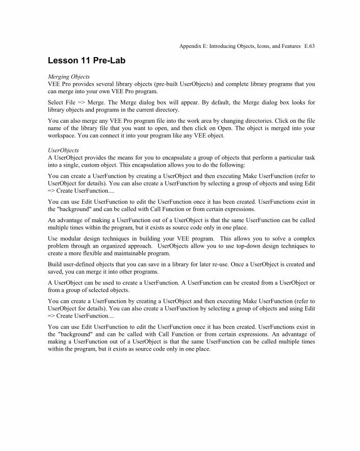
Appendix E: Introducing Objects, Icons, and Features E.63
Lesson 11 Pre-Lab
Merging Objects
VEE Pro provides several library objects (pre-built UserObjects) and complete library programs that you
can merge into your own VEE Pro program.
Select File => Merge. The Merge dialog box will appear. By default, the Merge dialog box looks for
library objects and programs in the current directory.
You can also merge any VEE Pro program file into the work area by changing directories. Click on the file
name of the library file that you want to open, and then click on Open. The object is merged into your
workspace. You can connect it into your program like any VEE object.
UserObjects
A UserObject provides the means for you to encapsulate a group of objects that perform a particular task
into a single, custom object. This encapsulation allows you to do the following:
You can create a UserFunction by creating a UserObject and then executing Make UserFunction (refer to
UserObject for details). You can also create a UserFunction by selecting a group of objects and using Edit
=> Create UserFunction....
You can use Edit UserFunction to edit the UserFunction once it has been created. UserFunctions exist in
the "background" and can be called with Call Function or from certain expressions.
An advantage of making a UserFunction out of a UserObject is that the same UserFunction can be called
multiple times within the program, but it exists as source code only in one place.
Use modular design techniques in building your VEE program. This allows you to solve a complex
problem through an organized approach. UserObjects allow you to use top-down design techniques to
create a more flexible and maintainable program.
Build user-defined objects that you can save in a library for later re-use. Once a UserObject is created and
saved, you can merge it into other programs.
A UserObject can be used to create a UserFunction. A UserFunction can be created from a UserObject or
from a group of selected objects.
You can create a UserFunction by creating a UserObject and then executing Make UserFunction (refer to
UserObject for details). You can also create a UserFunction by selecting a group of objects and using Edit
=> Create UserFunction....
You can use Edit UserFunction to edit the UserFunction once it has been created. UserFunctions exist in
the "background" and can be called with Call Function or from certain expressions. An advantage of
making a UserFunction out of a UserObject is that the same UserFunction can be called multiple times
within the program, but it exists as source code only in one place.

E.64 VEE Pro: Practical Graphical Programming
User Functions
There are three types of user-defined functions in VEE Pro.
UserFunction – It is a reusable segment of VEE code. There is only one copy of a particular
UserFunction in a VEE program. Therefore, you can access (call) it from various places within your
program. Changing a portion of your UserFunction automatically modifies all applications of that
UserFunction. You can call a VEE Pro UserFunction by using Menu Bar => Device => Call
(myFunction) or by using an expression within an object; an example would be from Formula.
UserFunctions can be either local or imported. You can also create libraries of UserFunctions for use
within other programs. You would import the UserFunction library. However, an imported
UserFunction cannot be edited. An imported UserFunctions can be called in a manner similar to the
calling of a local UserFunction.
Compiled Functions – A Compiled Function is a function written in another language, such as C or
C++. It is compiled into a dynamic linked library (DLL). You can load this library of compiled
functions into VEE Pro via the Import Library Object. Then you can call a compiled function via a
CALL Object or by writing an expression within a VEE Pro object. Note that, since these compiled
functions are loaded into VEE Pro, any errors or calling exit ( ) from a compiled function can cause
VEE Pro to crash. When there is insufficient memory allocation or memory is overwritten, it can cause
VEE Pro to randomly crash.
Remote Functions – A Remote Function is a VEE UserFunction that is running on another computer.
You can call a remote function the same way that you would call a UserFunction. However, the
remote function runs on a remote host computer that is connected to your network. This Remote
Function is specified via an Import Library Object.
Your new programs can be easily merged with existing VEE Pro programs using the Merge… command.
This command is in the File menu. When you use the Merge… command, you will see a list box that
displays the library (lib) subdirectory. This subdirectory is in the VEE Pro home directory. Merge is used
to copy an entire program into another program. Choose the UserFunction whenever you want to reuse
code. Thus, only one copy is retained. To copy UserFunctions from one program to another program, use
Menu Bar => File => Merge Library.

Appendix E: Introducing Objects, Icons, and Features E.65
Lesson 12 Pre-Lab
The Instrumentation Amplifier
The Instrumentation Amplifier (IA) amplifies the voltage difference across its input terminals. The IA
ideally applies no gain to identical signals that are simultaneously applied to both inputs; these signals are
known as common-mode signals. Common-mode voltages are caused by excessive return current from
various parts of the overall system via the IA signal-return conductor. The resulting error voltages can
easily mask the small output signals generated by many types of sensors. Proper (single-point) grounding
techniques are the usual solution.
The circuit of Figure 12.1 shows a conceptual model of the Instrumentation Amplifier. This circuit is used
in the next lab to show that the basis for common-mode rejection is simple subtraction. The
Instrumentation Amplifier is a differential amplifier with two identical gain channels of opposite sign. If
the same voltage is applied to both inputs, these voltages will cancel each other before arriving at the IA
output. See Figure 12.1 for the circuit wiring that is simulated in the laboratory experiment.

E.66 VEE Pro: Practical Graphical Programming
Figure 12.1. Instrumentation amplifier simulation showing common mode rejection
The instrumentation amplifier is widely used for interfacing sensor outputs to the next portion of a data
acquisition subsystem. It provides both temperature-stable, steady-state (dc) and dynamic (ac) performance
in addition to its high input impedance. This high impedance minimizes loading of the signal source and
instrument-amplifier gain. You can easily simulate the instrumentation amplifier in VEE Pro. You can then
use your simulation to explore the operation of both an ideal and non-ideal instrumentation amplifier.
K1 = +10X
K2 = -10X
Adder
K3 (A + B)
+Vin
-Vin
A = +K1 (+Vin)
B = -K2 (-Vin)
Sensor
Vcm
Common Mode Voltage Noise
Sensor Ground
Instrument Ground
Common Mode Voltage
Vout
where Vout = 10 [(+Vin) + (-Vin)]

Appendix E: Introducing Objects, Icons, and Features E.67
Understanding a Strain Gauge
Strain gauges indirectly determine strain by measuring the resistance change (∆R) on the structure being
monitored. As the force on the structure changes, the strain gauges on the same surface of the structure as
the applied force will increase in value while the strain gauges on the opposite surface will decrease in
value. See Figure 12.2.
FORCE
R + ∆R R + ∆R
R - ∆R R - ∆R
Strain gauge elements in extension;the resistance of each increases.
Strain gauge elements are in compression;the resistance of each decreases.
STRUCTURE UNDER TEST
RIGID
BEAM
Figure 12.2. The four strain gauge elements on a structure being deformed
The strain-gauge resistors (∆R) are connected electrically as a Wheatstone Bridge. The bridge excitation
voltage (VEXC) is the electrical input. The bridge electrical output (VBRIDGE) is the operational amplifier (op
amp) input. The relating equation is given in Figure 12.3. The op amp replaces a meter; its two inputs are
either above (+) or below (-) system ground.
The strain-gauge resistors compensate for the structure temperature. The stretching and shrinking of all
four resistors provide the differential-resistance change (∆R) that represents strain. The op amp provides
both circuit isolation and gain (K). The output voltage is VOUT = K x VBRIDGE. The output of the op amp is
connected to an n-bit analog-to-digital converter. The information provided to the data-acquisition system
is a digital word.

E.68 VEE Pro: Practical Graphical Programming
R + ∆R
R + ∆R R - ∆R
R - ∆R
VEXC
VBRIDGE Gain = K
V = V [∆R] RBRIDGE EXC
OUTVTo an analog-
to-digitalconverter
+
-
Figure 12.3. A four-element strain gauge network

Appendix E: Introducing Objects, Icons, and Features E.69
The VEE Pro-provided application programs
VEE Pro applications are located on the hard-drive location in the following sequence:
The Program Files folder,
The Agilent folder,
The VEE Pro 6.0 folder,
The examples folder, and
The Applications folder.
There are sixteen VEE Pro-supplied application simulations:
beam.vee* chaos.vee
coilspr.vee* convecoef.vee*
convert.vee digfilt.vee
fluidflw.vee lissajou.vee
mfgtest.vee* payback.vee
pid.vee simp_npv.vee
telecomm.vee torsion1.vee
torsion2.vee* wizbang.vee
The ones with the asterisk (*) are the ones explored in Lesson 12.
MATLAB®
VEE Pro 6 and higher access MATLAB® Script. This object is located in Menu Bar => Device.
MATLAB® programs can be written within the MATLAB® Script Object expression field. See Figure
12.4.
Figure 12.4. MATLAB® Script Object

E.70 VEE Pro: Practical Graphical Programming
Also, via the Function & Object Browser, MATLAB® functions can be accessed via the Type (left-hand)
column. Their major categories are listed in the Category (middle) column; the programs within each
category are located in the Function (right-hand) column. See Figure 12.5.
Figure 12.5. MATLAB® Function & Object Browser

Appendix E: Introducing Objects, Icons, and Features E.71
Lesson 13 Pre-Lab
Menu Bar => Display Spectrum (Freq)
There are four subheadings listed:
• Magnitude Spectrum
• Phase Spectrum
• Magnitude vs Phase (Polar)
• Magnitude vs Phase (Smith)
The subheading investigated in this lab is the Magnitude Spectrum icon. Its horizontal scale is frequency
(Freq). Its vertical scale is magnitude (Mag). Additional input terminals can be added to provide other
traces.
Horizontal variables are: scale name, auto scaling (on or off), maximum and minimum range, label
spacing, mapping (linear or logarithmic), log cycles, and scale color. These variables are accessed by a
single mouse click on Freq or via the Properties menu.
Vertical variables are: scale name, color, line type, and point type. These variables are accessed by a single
mouse click on Trace 1 or via the Properties menu.
The Time and Frequency Domains
Today, there are four generally accepted classes of waveforms that vary versus time:
• continuous
• discrete
• pulsating
• alternating
These waveforms may be periodic or non-periodic.
A continuous waveform varies from one moment to another; it does not change suddenly. Therefore, it
does not have a disruption in its waveform. Continuous waveforms are considered to be functions of time
because, for every value of time, they have only one value of voltage, current, or power.
A discrete waveform changes suddenly from its present value to another value at one or more points in
time. An example would be a series of steps or a “sawtooth” waveform.
A pulsating waveform changes quickly and then returns to its original value. Such a waveform may contain
one or more pulses. An impulse is an extreme example of a pulsating waveform.
Alternating waveforms vary from one moment to another; they may, or may not, change suddenly at any
moment of time. However, they “alternate” from a positive value to a negative value as time changes.
These waveforms may be functions versus time if they have only one vertical value for any given value of
time. They may be relations versus time if they may have more than one value of voltage, current, or power
for any given value of time.

E.72 VEE Pro: Practical Graphical Programming
When a sine-shaped waveform represents a voltage, the equation that describes this waveform is
e = Em sin α eq 13.1
where Em represents the maximum value (or peak) of the sine-shaped waveform and α represents the
angular displacement from the positive-X axis.
When the circular turning of any device is examined, it will generate a sine-shaped waveform. A sine-
shaped waveform displayed in the time domain can be graphed by projecting the tip of a line that rotates
with a circular motion. The circular display is graphed in polar coordinates; the projection of the tip of the
line is graphed in cartesian coordinates.
The mechanical velocity v of a device is usually expressed in revolutions per minute (rpm). It is often
converted to a frequency f whose unit is the cycle per second or Hertz. The relation between cycle per
second (Hertz) and angular velocity ω requires trigonometry:
ω = 2š radian
1 cycle · f
cycle
second = 2 š f
radian
second eq 13.2
The unit of angular velocity is the radian per second. As a math review, there are 2 radians or 360 degrees
in one mechanical revolution or one electrical cycle. Therefore
ω = 2 · · f eq 13.3
The frequency f of a sine-shaped waveform is related to its period T.
fcycle
second =
1
T
second
cycle eq 13.4
For the sine-shaped waveform whose base is zero, its one-period average height Eavg is zero because there
is as much area under the positive part of the waveform as there is under the negative part of the waveform.
However, the average value for one-half of a sine-shaped waveform can be derived. The result is:
Eavg
= 2
š E
m eq 13.5
The 2/ value is exact; many texts provide this value as 0.637 Em, which is approximately 2/ .
Power is the product of voltage E and current I. It continues to be the product of the instantaneous values
of voltage e and current i. Assume a voltage e and current i where
e = E sin (ωt + αe) eq 13.6
i = Im sin (ωt + αi) eq 13.7
where αe and αi are different initial phase angles for voltage (αe) and current (αi). Apply the
trigonometric identity:
sin A · sin B ≡1
2 cos A - B( ) -
1
2 cos A + B( ) eq 13.8
where A = ωt + αe and B = ωt + αi. The result becomes:
p = e · i = E
m I
m
2 cos α
e - α
i( ) -
Em
Im
2 cos 2 ω t + α
e + α
i( ) eq 13.9

Appendix E: Introducing Objects, Icons, and Features E.73
In the late 1880s, oscilloscopes did not exist. Thus, those who were experimenting with resistors,
capacitors, and inductors (such as Thomas Edison and Charles Steinmetz) could not observe the phase
differences. After many comparison experiments, Dr Steinmetz suspected there was a phase shift between
capacitor and inductor voltages and currents. He used calculus to investigate and verify the voltage-current
phase shift and other interactions. Interpretation is required as suggested by Dr Steinmetz:
• The first term is a constant and independent of time; time does not appear in this term. He named it
the average power value.
• The second term is time-dependent; its repetition rate is at twice the frequency of the original
voltage and current; its phase shift is the sum of αe and αi.
He then suggested that the first term be redefined by splitting the product of voltage and current into two
parts:
Em
2 ·
Im
2 = E · I eq 13.10
where E would be known as the effective value of voltage and I would be known as the effective value
of current. The word effective refers to the product of E and I; it would effectively represent the value
of useful power transferred from one location to another.
For Cartesian coordinates, the X axis is considered to be the domain of a function and the Y axis is
considered to be the range of that same function. (Recall that, for a function, there can be only one Y value
for each corresponding X value.) Therefore, the expression “time domain” indicates that the X-axis
(domain) label is replaced with the parameter: time. The Y axis (range) label may be replaced with either a
voltage – which is the most common – a current, or (seldom) a power. These displayed waveforms are
usually sine-shaped waveforms; they can be displayed on an oscilloscope.
The expression “frequency domain” indicates that the X-axis label is replaced with the parameter:
frequency. The Y axis (range) label is most often power because the display is usually associated with
spectrum analyzers. The frequency-domain waveform is usually one or more vertical lines, representing the
amount of power being transferred at that frequency. These vertical lines are usually displayed on a
spectrum analyzer.
A comparison of a sine wave displayed in the time domain (on an oscilloscope) and its frequency-domain
equivalent (displayed on a spectrum analyzer) is shown in Figure 13.1.

E.74 VEE Pro: Practical Graphical Programming
Figure 13.1. A Comparison of Time-Domain and Frequency-Domain waveforms
As noted earlier, the relation between the waveform period T and frequency f is:
f = 1
T eq 13.13
where f is measured in Hertz (cycles/second) and the period T is in seconds/cycle.
Include the entire unit for period. Most persons state the unit of period as time (in seconds). The unit that
belongs with a period computation is actually time/cycle or seconds/cycle. The importance of keeping the
entire and correct unit for a period will become more apparent whenever the Laplace Transform is applied.
The phase of the sine wave shown in Figure 13.2 is zero. (The frequency-domain display does not
normally indicate phase.) Dr Steinmetz “froze” the rotating line at t = 0. He devised a method for
correcting this shortcoming regarding phase difference; it also avoided calculus because he discovered that
engineers (and other technical people) in the United States were not comfortable working with calculus. He
examined mathematically the relations among voltage, current, and power, and how these relations could
be simplified if the calculus were reduced to algebra and trigonometry. He named the method: phasor
algebra, which is a shortened version of phase angle vector. He purposely avoided the word vector
because the rules for vector computations do not totally apply to phasor computations.
When working with phasor algebra, recall that:
A /α= A · ε jα eq 13.14
Therefore, phasor lengths are multiplied; phasor angles are added algebraically. The left side of this
equation is known as the polar form of a phasor; the right side of this equation is known as the exponential
form.
The relation between time and angle is
time (t)
2πω
voltage
0
Em
-Em
frequency (f or ω)
power
0 f or ω
avgP

Appendix E: Introducing Objects, Icons, and Features E.75
α = ω t = 2 f t eq 13.15
where α is measured in radians, ω in radians/second, t in seconds, and f in Hertz (which replaces the
cycle/second).
Note that ω is the frequency given in radians/second. Therefore, its relation with f in cycles/second (Hertz)
is
ω = 2 · · f eq 13.16
Once the computations (at t = 0) involving phasors were complete, the phasor line would be allowed to
rotate again. The resulting waveforms of voltage, current, and power would be the same. The phasor
approach included angle computations, which are not displayed on most spectrum analyzers. This was an
enormous step forward in the analysis of circuits involving resistors, capacitors, and inductors and, today,
electronic circuitry and operational amplifiers.
The use of the term frequency domain for phasor algebra is not quite correct. Dr Steinmetz described how
to compute the frequency-domain relations among voltage, current, and power. Then, after the analysis was
complete, he let the phasors rotate at those angular velocities that represented their original frequencies.
(Recall from above that the frequency of the power phasor would be at twice the frequency of the voltage
and current phasors.) As the voltage and current angular relations would remain the same, his
trigonometric analysis would apply for all of that time represented by the voltage and current phasors.
As the angle-domain (X-axis) should be shown horizontal, then the y = cos α waveform is rotated so its
angle axis is horizontal. The cosine-wave function is then also rotated. This is the way that the cosine-
shaped wave is usually displayed. The initial phase angle, α1, agrees with the positive-cosine reference
axis. Again, note that the phasor always rotates in a counterclockwise (CCW) direction.
The reference axes, used primarily by mathematicians and physicists, were suggested by Dr Steinmetz. A
positive angular motion is counterclockwise (CCW) from the phasor’s initial position. A negative angular
motion is clockwise (CW) from the phasor’s initial position. As more clocks and watches become digital,
these standards will become more difficult to remember. Use your imagination to visualize a car that is
passing in front of you from right to left. Its wheels will be rotating counterclockwise.
Periodic Waveforms and Their Fourier Series
In 1822 March 21, Jean Baptiste Joseph Fourier (1768-1830) published Analytical Theory of Heat where
he described how to analyze heat conduction in solids in terms of an infinite series of sine and cosine
terms, now known as a Fourier series. After reading that publication, Pierre Simon de Laplace (1749-1827)
criticized the work because it did not include relations as well as functions. Most mathematicians, at that
time, considered the omission to be trivial. Today, as technical personnel, we realize that its omission can
lead to difficulties in the analysis of certain periodic waveforms.
A non-sine-shaped periodic waveform can be expressed as a combination of sine and cosine waveforms.
Their frequency, amplitude, and phase angles will be directly related to the fundamental frequency of the
non-sine-shaped periodic waveform.
The most commonly expressed waveform is the “square” wave. For the square wave that starts (at t = 0),
its Fourier-series equation is:
square wave (ω) = sin ω + 1
3 sin (3ω ) +
1
5 sin (5ω) + … +
1
n sin (nω) eq 13.17

E.76 VEE Pro: Practical Graphical Programming
where n is an odd integer.
Note that the leading and trailing edges are multi-valued. They are not functions; they are relations.
Therefore, it is impossible to simulate a square wave exactly. Laplace was right!
Figure 13.2 further indicates that the frequency spectrum of a perfect sine-shaped wave is a function; it has
one vertical value for every horizontal time value. What will be the Fast Fourier Transform frequency-
spectrum magnitude presentation?
frequency60 Hz
p (usually)
time
e, i, or p
1/60 sec 1/30 sec0
Figure 13.2. The Time and Frequency Display for a sine-shaped wave
The Fast Fourier Transform (FFT) of this waveform will be displayed as shown in the “virtual” diagram of
Figure 13.3 because the FFT can only display functions, not relations.
frequency60 Hz
p (usually)
frequency60 Hz
p (usually)
actual virtual
Figure 13.3. A Frequency-Domain Display on a simulated spectrum analyser

Appendix E: Introducing Objects, Icons, and Features E.77
Observe three of the square-wave individual sinusoidal harmonics prior to being added to approach the
simulated square wave. See Figure 13.4.
Harmonics Added Harmonics Separated
Figure 13.4. Sinusoidal harmonics
Examine the right-hand oscilloscope presentation. It represents the separate first four waveforms:
harmonics 1, 3, 5, and 7, prior to their addition. (Reminder: The first harmonic is often referred to as the
“fundamental”.) The left-hand oscilloscope presentation represents the algebraic sum of these first four
frequencies.
Other commonly-applied waveforms in science, engineering, and technology include the periodic
triangular wave and the trapezoidal wave. The Fourier-series equation for the triangular wave is:
tri wave(ω ) = cos(ω) + 1
32
cos(3ω) + 1
52
cos(5ω ) + … + 1
n2
cos(nω) eq 13.18
The Fourier-series equation for the trapezoidal wave is:
trap wave(ω) = cos(ω ) - 1
32
cos(3ω ) - 1
52
cos(5ω) + … ±1
n2
cos(nω) eq 13.19
where the signs of the terms alternate every second term.
Other periodic waveforms that are considered applicable to science, engineering, and technology-oriented
problems are discussed in Tilton (1986) and Wei and Zhang (2000).

E.78 VEE Pro: Practical Graphical Programming
Lesson 14 Pre-Lab
Using Library Functions
The VEE Pro library functions are very flexible. You can
• use libraries via the VEE Pro UserFunctions,
• devise and merge a library of UserFunctions,
• devise a top-level program without programming the details of the UserFunctions,
• devise a report-generation program by building a VEE Pro program within that program,
• devise a new program that merges your newly created library of UserFunctions into it,
• import and delete the specific libraries that you select, and
• devise a program that will allow you to monitor several tests and note where any given test exceeds
previously established limits.
This flexibility will save you many hours of repetitious work.
Generating Lissajous Patterns
Lissajous patterns are generated by applying a reference sine-shaped wave to the X input of an X vs Y
display and applying a comparison sine-shaped wave to the Y input of that same display. When the two
frequencies are exact integers, then the Lissajous pattern becomes stationary. The frequency ratio is
determined by comparing the number of times the pattern is tangent to a horizontal line divided by the
number of times the pattern is tangent to a vertical line.
The amount of relative phase shift between the reference wave and the wave being compared changes only
the location of the tangent points but not their ratio. The phase shift can be computed from the equation:
sin θ = B/A, where
θ = the phase shift,
B = the value of the Y intercept (where X = 0), and
A = the value of the X intercept (where Y = 0).
The sign of the phase angle depends upon the quadrant in which it occurs.
The Junction (JCT) Object
The Junction Object offers two or more input terminals so the active input to a terminal may be passed on
to another object. The program must be such that only one Junction input terminal at a time is activated. It
can be used in feedback loops for data initialization.
The Call Object
This object executes a previously defined UserFunction, Compiled Function, or Remote Function.
The If/Then/Else Object
The If/Then/Else Object allows a branching of execution flow based upon the value on its input “If”
terminal. The input condition is tested to see if the input-pin information has not been met. If it has not
been met, then the Else terminal is activated with the zero value of the input expression. Additional “Else

Appendix E: Introducing Objects, Icons, and Features E.79
If” can be added. This action is different from a Comparison Object; the Comparison Object has an output
of either a one or a zero.
The Break Object
The Break Object terminates the current iteration loop. It usually operates along with the Until Break
Object.
The Until Break Object
This object causes execution to repeat until the Break Object is encountered.

E.80 VEE Pro: Practical Graphical Programming
Lesson 15 Pre-Lab
The VEE Pro Sequencer allows you to document tests, compare them against previously developed
specifications, and compare test runs with each other.
Accessing logged test data
The Sequencer output is a Record of Records. In the Sequencer record, each test uses the test name as its
field name. The fields within each test are named according to your logging configuration.
If you use the default configuration with the fields Name, Result, and Pass, you could access the result in
all of the test2 column with the notation Log[*].Test2.Result; see Figure 15.1.
Figure 15.1. A logged array of Record of Records
The Sequence Transaction dialog box
The following fields are available in the Sequence Transaction dialog box:
Sequence
Transaction Explanation
Field
TEST: The TEST: button toggles to EXEC.
The TEST: field holds the unique name used to
reference this test in the Sequencer. The default
names start with test1 and increment with each
test.
or:
Test 1
Test 1
Test 1
Test 1
Test 2
Test 2
Test 2
Test 2
Log [ 0 ]
Log [ 1 ]
Log [ 2 ]
Log [ 3 ]
Name
Result
Pass
Run 1
Run 2
Run 3
Run 4
Log [ * ]. Test 2. Result(* = 0, 1, 2 or 3)

Appendix E: Introducing Objects, Icons, and Features E.81
Sequence
Transaction Explanation
Field
Toggle TEST: to EXEC. The test will be
executed without a comparison of the test result
value; there is no logging of this test.
ENABLED ENABLED provides four menu choices:
ENABLED executes the test under all
conditions.
ENABLED IF: executes the test if the stated
expression is TRUE; used for audit test control.
DISABLED is the opposite of ENABLED.
DISABLED IF: is the opposite of ENABLED
IF.
Toggle the EXEC button to TEST.
SPEC NOMINAL: This provides the expected value from the test.
RANGE: RANGE signifies the range of PASS test values.
LIMIT uses just one test-data value for a
comparison.
Available are >, >=, <, <=, ==, !=
TOLERANCE Tolerance states the passing range of values by
adding or subtracting the specified tolerance to
the SPEC NOMINAL value.
%TOLERANCE % Tolerance states the
passing range of values by adding or subtracting
a percent tolerance to the SPEC NOMINAL
value.
FUNCTION: The FUNCTION: FIELD specifies which test to
run.
You may call
UserFunctions
Compiled Functions
Remote Functions
or:
You can write an expression to be evaluated.
Functions can be combined or nested.
Note: Advanced users should refer to the Sequencer Help menu and
explore additional variables.

E.82 VEE Pro: Practical Graphical Programming
Sequence
Transaction Explanation
Field
LOGGING ENABLED If logging is enabled, then this test logs a record.
If logging is disabled, then this test is not
logged.
For the LOGGING ENABLED mode, you can
choose the fields that you want logged if you
(a) close the Sequence Transaction dialog
box,
(b) open the Properties dialog box of the
Sequencer Object, and
(c) select the Logging tab, choosing from:
Name
Result
Nominal
High Limit
Low Limit
Pass
Time Stamp
Description
Name, Result, and Pass are the default
selections.
IF PASS IF PASS tells VEE Pro to branch,
according to your selection, to THEN
CONTINUE.
IF PASS CALL: IF PASS CALL tells VEE Pro to call the
specified function (or any expression) if your
test passes and THEN CONTINUE.
IF FAIL IF FAIL tells VEE Pro to branch, according to
your selection, and THEN CONTINUE.
IF FAIL CALL IF FAIL CALL tells VEE Pro to call the
specified function (or any expression) if your
test passes and THEN CONTINUE.
Note: The fields “THEN CONTINUE” are available for IF PASS, IF PASS CALL,
IF FAIL, and IF FAIL CALL.

Appendix E: Introducing Objects, Icons, and Features E.83
THEN CONTINUE THEN CONTINUE executes the next
test configured in the Sequencer.
THEN RETURN tells VEE Pro to stop
executing tests and put the specified expression
on the Return output pin of the Sequencer.
THEN GOTO: jumps to the test named in its
field.
THEN REPEAT repeats the current test up to
the number of times specified in the MAX
TIMES: field.
If the PASS/FAIL condition still exists after the
maximum number of repeats, then VEE Pro
continues with the next test.
THEN ERROR: stops execution by generating
an error condition with the given error number.
An error can be trapped with the error output
pin on the Sequencer.
THEN EVALUATE: calls the specified User
Function (or any expression) which must return
a string that states a branching menu option.
Valid string results are:
“Continue”
“Return <expr>”
“Goto <name>”
“Repeat <expr>”
“Error <expr>”
where <expr> is any valid VEE Pro
expression and <name> is the name of
the test in the sequence. This powerful
option allows you, via the program, to
ask the user what to do next.
DESCRIPTION: Holds your Text comments; they appear on the
Sequencer transaction bar and can be stored
with your test record by using the Logging tab
in the Properties dialog box.
Declaring Globals
Globals can be declared as a specific type and shape or you can use the SetVariable Object to create an
undeclared global.
• Declared variables allow you to set their scope so they will be truly global. They can also be local
to a UserFunction, UserObject, or local to a library of UserFunctions.
• Declared variables also allow the VEE compiler to perform type checking; it will run slightly
faster.
Using undeclared globals is recommended for the situations where declared variables are not supported,
such as a Record of Records.

E.84 VEE Pro: Practical Graphical Programming
Lesson 16 Pre-Lab
Data Selection Control
There are six Data Selection Control icons accessed via Menu Bar => Data => Selection Control. See
Figure 16.1; each provides a method of accepting operator input where a single value is chosen from a list
of possible values. Their display formats vary; however, they all execute in the same manner.
Figure 16.1. The six Data Selection Control objects
Use Selection Control objects either to set a constant or to receive a user input from a list of choices. The
first item in the list is assigned ordinal position 0; the nth item in the list is assigned ordinal position n-1.
To use a Selection Control as a prompt, change the name of its object to a prompt such as "Make a
Selection:" and place it on or add it to an existing user panel.
Each object menu offers Edit Enum Values; it allows you to either add valid selections to the enumerated
list of choices or edit the names of existing choices. First, add a choice, then press the Tab key to move to
the next entry in the list. You can move back up in the list by pressing Shift+Tab or by clicking the mouse
to remove the blinking vertical cursor.
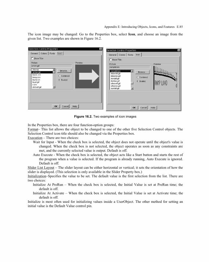
Appendix E: Introducing Objects, Icons, and Features E.85
The icon image may be changed: Go to the Properties box, select Icon, and choose an image from the
given list. Two examples are shown in Figure 16.2.
Figure 16.2. Two examples of icon images
In the Properties box, there are four function-option groups:
Format– This list allows the object to be changed to one of the other five Selection Control objects. The
Selection Control icon title should also be changed via the Properties box.
Execution – There are two choices:
Wait for Input - When the check box is selected, the object does not operate until the object's value is
changed. When the check box is not selected, the object operates as soon as any constraints are
met, and the currently selected value is output. Default is off.
Auto Execute - When the check box is selected, the object acts like a Start button and starts the rest of
the program when a value is selected. If the program is already running, Auto Execute is ignored.
Default is off.
Slider List Layout – The slider layout can be either horizontal or vertical; it sets the orientation of how the
slider is displayed. (This selection is only available in the Slider Property box.)
Initialization–Specifies the value to be set. The default value is the first selection from the list. There are
two choices:
Initialize At PreRun – When the check box is selected, the Initial Value is set at PreRun time; the
default is off.
Initialize At Activate – When the check box is selected, the Initial Value is set at Activate time; the
default is off.
Initialize is most often used for initializing values inside a UserObject. The other method for setting an
initial value is the Default Value control pin.
E.86 VEE Pro: Practical Graphical Programming
Control inputs may be added for the following:
The Default Value input allows you to change the current value. This input requires a Text Scalar value
(or any data that can be converted to a Text Scalar, including an Enum). This value must match one
of the possible Enum values (case sensitive).
The Reset input allows you to programmatically set the current value to the first (0 ordinal) value in the
list. The actual data on the Reset input is ignored.
The Enable Editing and Disable Editing inputs allow you to control whether the values can be changed
in the object’s open view.
The Enum Values input allows you to set the list of possible values for the Selection Control. This
input requires Enum, a Text Array 1D, or any data that can be converted to a Text Array.
Enum Containers are automatically converted into Text for many objects, including Collector,
Concatenator, Sliding Collector, and most Formula objects.
Ordinal Value: You may connect a line to the Ordinal output rather than to the selected string, or you
can use the ordinal(x) function on the Enum.
The six Data Selection Control objects each operate differently:
Radio Buttons – The choices are all displayed. The selection is made when the radio button next to the
choice is pressed.
Cyclic Button – The choices cycle as the button field is clicked on. This choice is best used if there are
two choices such as On/Off or Stop/Go or in a dialog box where the choice is confirmed by another
button.
List – The choices are presented in a list box with scroll bar if all choices cannot be shown at once. The
selection is made when the choice is clicked on.
Drop-Down List – The choices are presented in a list box that drops down when the arrow to the right
of the field is pressed. The selection is made when the choice is clicked on.
Pop-Up List – The enumerated choices are presented in a list box in a dialog box that is displayed when
the button field is pressed. The selection is made when the choice is clicked on and OK is pressed.
Slider List – The choices are presented as “tic” labels on a slider. The selection is made when the slider
button or the label is clicked on.
To/From Files may be compared with other To/From Objects:
To/From DataSet – It is a combination of To/From File, To DataSet, and From DataSet. It is simpler to
use and less error-prone in retrieving data; however, it is slower than To/From File since more
description of field names, field types, and data must be written.
To/From File Read/Write Container – It is simpler to use than To/From File; however, it requires more
disk storage space and is slower to execute because of the extra descriptive information required.
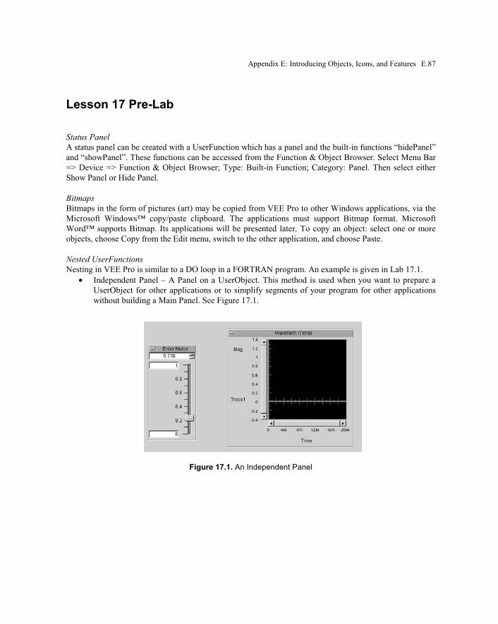
Appendix E: Introducing Objects, Icons, and Features E.87
Lesson 17 Pre-Lab
Status Panel
A status panel can be created with a UserFunction which has a panel and the built-in functions “hidePanel”
and “showPanel”. These functions can be accessed from the Function & Object Browser. Select Menu Bar
=> Device => Function & Object Browser; Type: Built-in Function; Category: Panel. Then select either
Show Panel or Hide Panel.
Bitmaps
Bitmaps in the form of pictures (art) may be copied from VEE Pro to other Windows applications, via the
Microsoft Windows™ copy/paste clipboard. The applications must support Bitmap format. Microsoft
Word™ supports Bitmap. Its applications will be presented later. To copy an object: select one or more
objects, choose Copy from the Edit menu, switch to the other application, and choose Paste.
Nested UserFunctions
Nesting in VEE Pro is similar to a DO loop in a FORTRAN program. An example is given in Lab 17.1.
• Independent Panel – A Panel on a UserObject. This method is used when you want to prepare a
UserObject for other applications or to simplify segments of your program for other applications
without building a Main Panel. See Figure 17.1.
Figure 17.1. An Independent Panel

E.88 VEE Pro: Practical Graphical Programming
• Pop-Up Panel – A panel on a UserObject with Show (Panel) on Execute specified via the
Properties dialog box. This method is usually used for custom dialog boxes that query for
information, and then go away. This type of panel pops up anywhere you desire in a VEE Pro
window. See Figure 17.2.
Figure 17.2. The “Enter Frequency” Pop-Up Panel
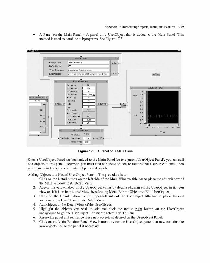
Appendix E: Introducing Objects, Icons, and Features E.89
• A Panel on the Main Panel – A panel on a UserObject that is added to the Main Panel. This
method is used to combine subprograms. See Figure 17.3.
Figure 17.3. A Panel on a Main Panel
Once a UserObject Panel has been added to the Main Panel (or to a parent UserObject Panel), you can still
add objects to this panel. However, you must first add these objects to the original UserObject Panel, then
adjust sizes and positions of related objects and panels.
Adding Objects to a Nested UserObject Panel – The procedure is to:
1. Click on the Detail button on the left side of the Main Window title bar to place the edit window of
the Main Window in its Detail View.
2. Access the edit window of the UserObject either by double clicking on the UserObject in its icon
view or, if it is in its restored view, by selecting Menu Bar => Object => Edit UserObject.
3. Click on the Detail button on the upper-left side of the UserObject title bar to place the edit
window of the UserObject in its Detail View.
4. Add objects to the Detail View of the UserObject.
5. Highlight the objects you wish to add and click the mouse right button on the UserObject
background to get the UserObject Edit menu; select Add To Panel.
6. Resize the panel and rearrange these new objects as desired on the UserObject Panel.
7. Click on the Main Window Panel View button to view the UserObject panel that now contains the
new objects; resize the panel if necessary.

E.90 VEE Pro: Practical Graphical Programming
Adding a UserObject Panel to the Main Panel:
1. Right-click on the UserObject in the Detail View of the Main Window; select Restore. (The
UserObject will expand into the Edit window of the newly created Panel.)
2. Highlight the UserObject to be added to the panel; select Edit; Add To Panel via a right-mouse
click. You can nest a UserObject Panel on its UserObject Panel by following the same steps above,
except you must use the Edit menu of the identified UserObject.
3. Change its size, location, and other appearance details as desired.
Note: When you nest a panel on another panel, you are making a copy of its panel contents. The
copy is linked to the original panel and is locked. You must make all changes to the original
UserObject Panel; the copy is automatically changed.
An Overview of Filter Theory
Filters are the name given to the class of circuits that affect the various frequency components of an input
signal in a different manner. Filters are also referred to as "selective circuits" in the literature.
Modern filter (selective-circuit) design requires an understanding of:
• the Transfer Function of a circuit
• the Laplace Transform derivation of that Transfer Function
• the response of a filter to step and impulse input signals
• the frequency-domain response to sine-shaped input signals
• the relation between pulse time delay and sine-wave phase shift
These topics are reviewed below.
Filter Design Procedure
The customary approach to filter design is to
1. Determine the filter transfer function H(s).
The transfer function H(s) is defined as the ratio of the filter output voltage Eo(s) to the filter input
voltage Ei(s). It is assumed that there is no loading upon the output caused by the next connected
circuit.
H(s) = E
o(s)
Ei(s)
where Io(s) = 0 eq 17.1
2. Locate all poles and zeros on the "s" plane.
The poles are the denominator zeros; the zeros are the numerator zeros.
3. Convert H(s) to H(jω).
Replace “s” with “jω” everywhere.
j = -1 eq 17.2
j2 = -1 eq 17.3
j3 = - -1 eq 17.4
j4 = + 1 eq 17.5
Recall that, from the algebra , these exponents repeat every four integers; the “j” is cyclic.

Appendix E: Introducing Objects, Icons, and Features E.91
4. Group separately the real and “j” terms for both the numerator and the denominator.
5. Select component values.
Choose values that will not load the previously connected circuit.
Choose values that will not be loaded by the next connected circuit.
6. Compute and graph |H(jω)| and /H(jω).
The magnitude – |H(jω)| – is determined by applying the Pythagorean Theorem separately to the
numerator and the denominator if there are both real and imaginary values. The magnitude is the
ratio of these two separate computations.
The angle – /H(jω) – is the difference between the numerator angle and the denominator angle.
Each angle is computed by applying the trigonometric formula:
θ = invtan imaginary group of terms
real group of terms eq 17.6
where the proper quadrant for each angle must be included in the solution.
7. Return to H(s) and examine transients, where important.
Note: Transients prevent correct filter behavior for at least 5τ seconds, where the τ is obtained
from the denominator of H(s); it is the largest value of time in the expression.
Filter component-content classifications
Filters are first classified according to the types of components they contain.
a. Passive filters consist of resistors, capacitors, resonators, piezoelectric crystals, and (sometimes)
inductors. Passive filters operate best in the mid-audio frequency range. Passive filters that contain
inductors may become design-implementation problems because of the inductor physical
characteristics. If the resistance of the inductor is to be ignored, then the physical size of the
inductor may become too large for the system. If the physical size of the inductor is to be designed
to be smaller, then the resistance of the inductor must be included in the design. Then the
interwinding capacitance of the inductor may become a problem. Radio-frequency-band (RF)
filters consist of small inductors constructed with wire of a very small diameter. The coils are
wound so the interwinding capacitance may be ignored. At "radio" frequencies, the inductive
reactance of the coil is large when compared to the coil internal resistance.
b. Active filters consist of magnetic amplifiers, transistor amplifiers, or operational amplifiers for the
active components; they also consist of resistors and capacitors; they seldom contain inductors
unless the active component is a magnetic amplifier. Active filters require at least one power
supply for the active components. Feedback connections are usually part of the topology of active
filters. Thus an active-filter design may be unstable; it may suddenly oscillate. Active filters
operate best from 0 < f < 100 kHz where this upper value of frequency is increasing annually as
operational-amplifier designs improve.
Frequency-range (ideal) classifications and terminology
Filters are next classed according to their effect upon the sine-shaped input frequencies. For ideal filter
configurations (topologies) consisting of a large number of (Laplace) poles, either the frequencies are
passed with no attenuation, or the frequencies are rejected with maximum ("infinite") attenuation. See
Figure 17.4.
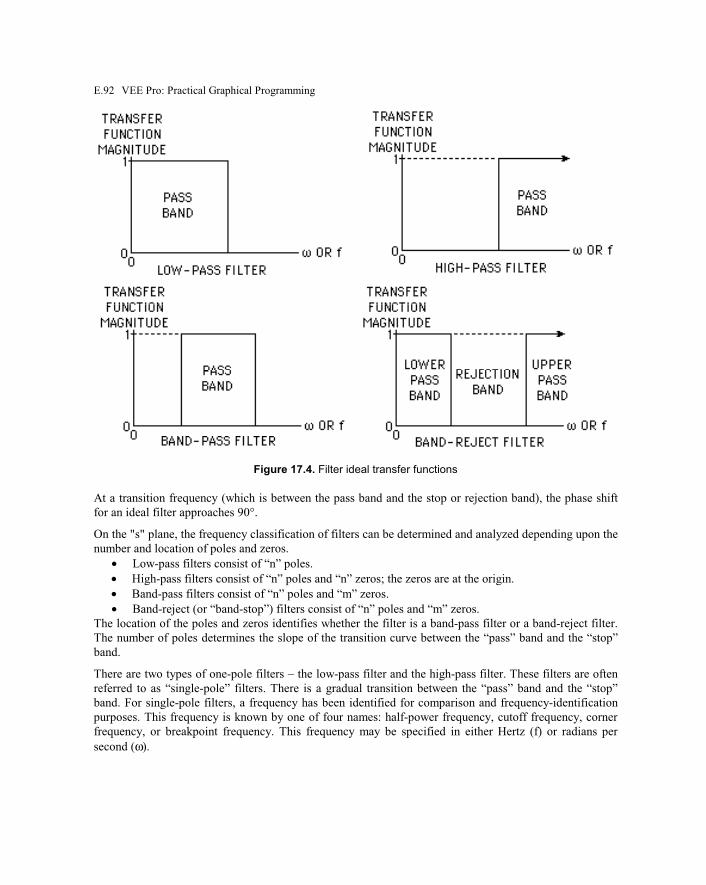
E.92 VEE Pro: Practical Graphical Programming
Figure 17.4. Filter ideal transfer functions
At a transition frequency (which is between the pass band and the stop or rejection band), the phase shift
for an ideal filter approaches 90°.
On the "s" plane, the frequency classification of filters can be determined and analyzed depending upon the
number and location of poles and zeros.
• Low-pass filters consist of “n” poles.
• High-pass filters consist of “n” poles and “n” zeros; the zeros are at the origin.
• Band-pass filters consist of “n” poles and “m” zeros.
• Band-reject (or “band-stop”) filters consist of “n” poles and “m” zeros.
The location of the poles and zeros identifies whether the filter is a band-pass filter or a band-reject filter.
The number of poles determines the slope of the transition curve between the “pass” band and the “stop”
band.
There are two types of one-pole filters – the low-pass filter and the high-pass filter. These filters are often
referred to as “single-pole” filters. There is a gradual transition between the “pass” band and the “stop”
band. For single-pole filters, a frequency has been identified for comparison and frequency-identification
purposes. This frequency is known by one of four names: half-power frequency, cutoff frequency, corner
frequency, or breakpoint frequency. This frequency may be specified in either Hertz (f) or radians per
second (ω).

Appendix E: Introducing Objects, Icons, and Features E.93
One-pole filters are either high-pass filters or low-pass filters. Examples of the only possible two
topologies for one-pole (passive) filters are given in Figure 17.5.
Figure 17.5. One-pole filter options

E.94 VEE Pro: Practical Graphical Programming
Note that these one-pole filters can be identified by their Laplace-World descriptions.
• A low-pass filter consists of one pole
• A high-pass filter consists of one pole and one companion zero at the origin
In the frequency domain, the range of the angle is 90 degrees.
Two-pole filters can be low-pass, high-pass, band-pass, or band-reject filters. The only possible four
topologies for two-pole (passive) filters are given in Figure 17.6.

Appendix E: Introducing Objects, Icons, and Features E.95
Figure 17.6. Two-pole filter options

E.96 VEE Pro: Practical Graphical Programming
Note that these two-pole filters can be identified by their Laplace-World descriptions.
• A low-pass filter consists of two poles.
• A high-pass filter consists of two poles and two companion zeros at the origin.
• A band-pass filter consists of one pole at a low frequency (near the origin), a companion zero at the
origin, and one pole at a high frequency.
• A band-reject filter consists of one pole at a high frequency with a companion zero and also one
pole at a low frequency.
In the frequency domain, the range of the angle value is 180 degrees for a two-pole filter.
Filters may contain both inductive (L) and capacitive (C) components, or their equivalent – an operational
amplifier may be used to simulate an inductor. The math derivations indicate that these filters may have
characteristic curves that deviate from the modern conventional RC implementations. This deviation can
be explored by examining the solution to the standard quadratic equation for a two-pole filter.
as2 + bs + c = 0 eq 17.7
where
s = - b ± b
2 - 4ac
2a eq 17.8
Whenever the discriminant (b2 - 4ac) is negative, there will be a peak in the magnitude-versus-frequency
curve at the “resonant” (ω0) frequency of the transfer function. This is the frequency at which the angle (or
phase shift) of the transfer function is zero.
Filter Specifications
As noted above, a filter can be specified by its number of poles.
• A one-pole filter can be only one of two types – high-pass or low-pass.
• The "sharpness" of its magnitude-versus-frequency curve is gradual when compared to an ideal
filter curve.
Increasing the components within a filter can cause the actual filter curve to approach the curve of an
"ideal" filter.
The specification of these filters requires additional parameters and their companion definitions.
a. The number of poles and, where applicable, the number of zeros
The location of these poles and zeros specifies the filter classification and the shape of its
magnitude and phase (versus frequency) curves.
b. The half-power (cutoff, corner, or breakpoint) frequency or frequencies
These frequencies specify a defined gain (or attenuation) level at which one-half the normal
pass-band power is transferred from input to output.
c. Attenuation (and gain) levels
There are three possible attenuation (or gain) specifications.
1. Absolute Attenuation or Gain
2. Relative Attenuation or Gain
3. Attenuation or Gain Floor

Appendix E: Introducing Objects, Icons, and Features E.97
d. Pass Band Ripple
This parameter specifies the amount of allowable deviation of the "magnitude" curve from the
desired (or normal) value.
e. Group Delay
This parameter is the derivative of phase-shift versus frequency.
f. Group Delay Ripple or Tolerance in Group Delay
This parameter specifies the amount of allowable deviation of the "phase shift" curve from the
desired (or normal) value.
g. Step Response
This parameter specifies the output of a filter to a step input. The step response normally
includes deviation amounts or percentages from the specified curve.
h. Impulse Response
This parameter specifies the output of a filter to an impulse input. The impulse response
normally includes deviation amounts or percentages from the specified curve.
Filter Types
There are several types or classifications of filter designs. The filter types have often been given the name
of the designer first associated with the design description as documented in the literature. The most
common types are
1. Butterworth
2. Chebyshev (Tschebyschev)
3. Bessel (Maximally Flat Time Delay, or MFTD)
4. Cauer Elliptic
5. Switched Capacitor
6. Paynter
7. Thompson
8. Gaussian
9. Equi-Ripple Group Delay
Information regarding these filter types is available in the bibliography.
Specific Filter Designs
Filter designs require investigation of the location of poles and zeros on the “s” plane and the magnitude
and frequency response in the frequency domain. Information regarding the Laplace-World “s” plane and
the Steinmetz frequency domain (ω) is given below.
Butterworth Filter Design: A Butterworth filter has a relatively flat magnitude response in its
frequency-domain pass band. The pole/zero “s” plane, two-dimensional diagram for a four-pole
Butterworth filter design has, as its locus of pole locations, a semi-circle.
Chebyshev (Tschebyschev) Filter Design: A Tschebychev filter has a variable-magnitude (ripple)
response in its frequency-domain pass band. The pole/zero “s” plane, two-dimensional diagram for a
four-pole Tschebychev filter design has, as its locus of pole locations, an ellipse.
Bessel (Maximally Flat Time Delay, or MFTD) Filter Design: A Bessel filter has a smaller variable-
magnitude (ripple) response in its frequency-domain pass band than does the Tschebychev filter. The
pole/zero “s” plane, two-dimensional diagram for a four-pole Bessel filter design has, as its locus of
pole locations, an ellipse.

E.98 VEE Pro: Practical Graphical Programming
Cauer Elliptic: A Cauer Elliptic filter has a relatively flat magnitude response in its frequency-domain
pass band. The pole/zero “s” plane, two-dimensional diagram for a four-pole, four-zero Cauer Elliptic
filter design also has, as its locus of pole locations, an ellipse.
Note: The zeros of the Cauer elliptic filter are no longer at the origin.
Switched Capacitor Filter Design: A switched-capacitor filter utilizes a clock to achieve an ω0 that is a
variable. The value of ω0 is controlled by a digital “clock” whose frequency can be accurately
controlled.
In the 1950’s, R. P. Sallen and E. L. Key devised a filter using an operational amplifier (op amp). Such a
filter is referred to as an “active” filter because it contains an active component which, in this
implementation, is an op amp.
Typically, each desired filter pole requires one op amp. This one-pole-per-op-amp approach allows for
much simpler circuit and system analysis. The op amp acts as a circuit isolator. Thus the location and
effect of each pole can be computed separately.
Active filters require no inductors, thus saving large amounts of space. Also, active filters usually perform
more efficiently and effectively then do their passive-filter counterparts.
A second-order, Sallen-Key, low-pass filter topology requires one (isolating) op amp. This topology is
shown in Figure 13.8. Its transfer function is given in the article by Mark Fortunato using the same
component notation as shown in Figure 17.7.
Figure 17.7. A Sallen-Key low-pass filter topology
Resistors with tolerances of 5% can be used with this Sallen-Key topology.
If a high-pass Sallen-Key filter is desired, then resistors R1 and R3 are replaced by capacitors C1 and C3;
capacitors C2 and C4 are replaced by resistors R2 and R4. The spread in frequency response for the high-
pass filter is much “tighter” than that of the low-pass filter. In practical applications, 1%-tolerance resistors
and 5%-tolerance capacitors are used because of their availability. This also keeps the total circuit cost
under control.
Active filter circuits can be designed and constructed with ten or more op amps. Because the op amps act
as circuit isolators, the circuit analysis requirement seldom exceeds two equations per op-amp stage and
often only one equation per stage. The application of one of Kirchhoff’s two Laws is all that is required.
VIN VOUT
R1
C2R3
C4
RA RB

Appendix E: Introducing Objects, Icons, and Features E.99
The overall transfer function for the filter/op-amp stages is the product of each individual transfer
functions derived separately. Thus, the math becomes tolerable and transient analysis can be included.
Computer programs that can process the Laplace “s” are not yet available to the designer.
Filters can be designed using easy-to-purchase, off-the-shelf components. Filters can also be purchased as
individual components. Because these off-the-shelf designs usually employ inexpensive op amps, they
often require two power supplies: +15Vdc and -15Vdc.
It is possible to purchase active filters that require a single (positive) power supply. The filter design can
be adapted to the op-amp power-supply requirements that you are using for the remainder of your system.
Thus, your spare-parts inventory can be kept to a more reasonable level.
A number of excellent references regarding filters are given in the bibliography.
This completes the pre-labs for the first seventeen lessons. There is no pre-lab for Lesson 18 because it
describes how to optimize the labs in the previous seventeen lessons.

Appendix F
Agilent VEE 7.0 Features
VEE 7.0 has some new and unique features. They are described below under the headings: Undo and
Redo, Saving Programs, Object Property Editing, Rich Text Format, Visual Studio.NET, Object Property
Editing, Panel Edit Features, Using .NET Assemblies, Connectivity for LAN and USB Based Instruments,
.NET and IVI-COM Drivers, Error Codes, Terminology, VEE and the .NET Framework, .NET and
Communications, and VEE and .NET Security.
Undo and Redo
For Undo, use (Ctrl + Z) or Select Menu Bar => Edit => Undo or click the Task Bar Undo symbol.
One of the most commonly requested features has been Undo. Both Undo and Redo operations will be
supported in VEE for certain common operations. Examples include: cut a line, delete a terminal, delete
objects from a panel, paste objects, and move an object. Undo/Redo will not be available for every
operation in VEE 7.0. The following are available on Undo/Redo:
Panel – Align, delete, and move or group single objects.
• Detail – Cut or paste objects; move, align or delete a line; add, delete or modify a terminal; add or
delete a terminal on a UserObject or UserFunction; and autoscroll.
• Undo and Redo taskbar icons have toolkit help that helps you understand what you are undoing or
redoing.
You can only undo the most current operations.
For Redo, use (Ctrl + Y) or Select Menu Bar => Edit => Redo or from the Task Bar Redo symbol.
Redo is available only for operations supported by Undo. See Undo and Redo Help menu.
Saving Programs
VEE 7.0 has some new features, such as the Property Grid and Microsoft Visual Studio .NET
programmability that cause the VEE 7.0 save format to be unique. Programs saved from VEE 7.0 will not
load into prior VEE versions.

F.2 VEE Pro Practical Graphical Programming
Object Property Editing (Select Menu Bar => View => Properties)
VEE provides a Properties window where you can easily change properties of your VEE objects. To
access the Properties window, click on the Object It also operates when you select multiple objects
(providing an "intersection" of properties for the objects if they are different). It works for both the Detail
View and Panel View. Any changes made in the Property window in the Panel View affect only the Panel
View of that object. It may not be available for all objects. See Figure F.1. See Properties (Object) Help
menu for further details.
Figure F.1. Properties window
Panel Edit Features
The following are some of the features that have been added: visible grid, alignment of objects, "rubber-
band" selection of objects (Ctrl while dragging the objects), undo of most common operations while
building a panel, bring to front, send to back, and tab order.
Rich Text Format (RTF) for Note Pad and Description
Using the capability of .NET, RTF has been implemented for the Note Pad and Descriptions. Additionally,
the notes and descriptions support automatic hyperlink detection and will start your browser when you
click a link. Both of these support Undo (CTRL + Z) and Redo (CTRL + Y) and other editing short-cut

Agilent VEE 7.0 Features F.3
keys. You can cut and paste from the .RTF file directly into a note or description or from the description
directly to the .RTF file. Text will word-wrap also.
Visual Studio.NET and the .NET Framework-Based Class Library
Visual Studio .NET is Microsoft’s latest development environment. It addresses the needs of both
programmers and World Wide Web developers. From a VEE perspective, the strength of .NET is the
Framework Class Library. The .NET Framework is distributed with VEE 7.0. There is a description of
.NET and the .NET Framework at:
http://msdn.microsoft.com/netframework/technologyinfo/overview/default.aspx.
The CLR provides common services for .NET Framework applications. Most languages are supported by
the CLR. Many time consuming and awkward programming tasks are performed automatically by the
CLR. Examples include: memory management, exception handling, and security management.
The .NET Framework also includes a common class library. These object-oriented classes are integrated
into the CLR. The standard class library is an asset from which your managed code can derive
functionality; the standard type library brings consistency across programming languages. Some of the
types available help with tasks such as file and string management.
.NET provides a native COM interop technology. This means that a COM component can be accessed as a
.NET object and a .NET object can be accessed as a COM component.
Using .NET Assemblies
For access to .NET capabilities, VEE 7.0 provides sources of .NET classes:
• The Microsoft .NET Framework Library and
• Third-party .NET libraries and .NET classes.
See the .Net (DotNet) examples directory to explore the power of the .NET Framework.
An additional feature is its ability to import namespaces. From the Device => .NET Assembly References
menu, mark the "Import namespaces after closing" checkbox. (To use an Assembly, you must add a
reference to it.) Choose one or more .NET Assemblies; you will be prompted to select zero or more
namespaces. You can also choose Import .NET Namespaces from the Device menu. This avoids
performing a namespace import; System.IO.File.Exists() simplifies to File.Exists() when you import
System.IO. With a namespace import, your method becomes File.Exists() which reduces typing.
There is a new “type conversion” function known as “asClrType”. This function converts a VEE data type
to a .NET/CLR data type. These data types include primitive, decimal, DateTime, and String. See
examples\datetime.vee in the Agilent VEE Examples programs.
Connectivity for LAN and USB Based Instruments
The VEE I/O subsystem continues to be enhanced to allow for interaction with devices (T&M Industry
standard) that are connected via LAN (VXI-II) and the Universal Serial Bus (USB). These connectivities
are becoming standard throughout the industry.

F.4 VEE Pro Practical Graphical Programming
.NET and IVI-COM Drivers
IVI-COM is a new standard for instrument compatibility. Established by the IVI Foundation, it encourages
instrument manufacturers to design instruments that are interchangeable with their competitors. The IVI
Foundation is a consortium established to promote specifications for programming test instruments. For a
review of the IVI Foundation, go to http://www.ivifoundation.org/.
To adapt to these new standards, VEE accepts all Agilent IVI-COM drivers as well as third-party IVI-
COM drivers. VEE interacts with IVI-COM drivers by finding a Primary Interop Assembly (PIA). An
assembly is an .EXE or DLL file and is the fundamental building block of a .NET application. The PIA is a
.NET assembly provided by vendors for their COM-based components. Because the VEE IVI-COM driver
is a COM-based component, VEE will either search for a PIA or attempt to create one. You can then use
the IVI-COM driver just like any other .NET assembly. They will eventually be integrated into the VEE
Instrument Manager.
To obtain drivers for your instruments, go to http://www.agilent.com/find/adn. If you are an ADN member,
select IVI-COM and VXIplug&play drivers can be located in the Downloads area of ADN (Agilent
Developers Network). If you are not an ADN member, it is an online source for Agilent drivers, evaluation
software, documentation, and white papers. To sign up for this free service, fill out the registration form
for new users. Once the IVI-COM drivers are installed and registered on your system, they are available
just like any other COM component and, like most COM components, will appear on the COM tab of the
Device = > .NET References in VEE. Choose your driver from the assemblies by using the Function &
Object Browser with the COM tab. This includes choosing the driver class; constructing the driver in the
VEE program; initializing it; and using the properties, events, enumerations, and methods associated with
it[0] This is only true for drivers that support the IVI Class Compliant interface. IVI-COM drivers can have
two interfaces: the IVI COM Class Compliant and the Instrument Specific Interface.
The Class Compliant one is defined by the IVI Foundation and should work with any instrument of the
same type. The instrument specific interface will only work with one specific instrument. The instrument
specific interface would support more features available in the specific instrument. For example, if two
vendors provide an IVI-COM driver for a DMM to meet the IVI standard, the base drivers must be
interchangeable. This means that whichever driver you use on your system, the DMMs from either vendor
will work. Any vendor’s DMM will work using the class compliant interface; the Agilent DMM will work
with the Agilent driver instrument specific interface. Your code is automatically reusable. Via .NET’s
interop technology, the IVI-COM drivers become available to VEE which then adds the Assembly
Reference to the Function & Object Browser’s .NET Object Assembly References list.
Error Codes
All VEE 7.0 error codes are available on the Internet and can be downloaded from http://www.agilent.com.

Agilent VEE 7.0 Features F.5
Terminology
Assembly. Microsoft defines an Assembly as follows: “Components are packaged in assemblies.
Assemblies are the reusable, versionable, self-describing building blocks of .NET applications. The
simplest assembly is a single executable that contains all the information necessary for deployment and
versioning. An Assembly is the fundamental building block of the .NET Framework. It takes the form of an
executable (.exe) or dynamic link library (.dll) file.”
Primary Interop Assembly (PIA). Microsoft defines a PIA as follows: “A primary interop assembly is a
unique, vendor-supplied assembly that contains type definitions (as metadata) of types implemented with
COM. There can be only one primary interop assembly, which must be signed with a strong name by the
publisher of the COM type library.”
Namespace. Microsoft defines a Namespace as follows: “.NET Framework types use a dot syntax naming
scheme that connotes a hierarchy. This technique groups related types into namespaces so they can be
searched and referenced more easily. The first part of the full name - up to the rightmost dot - is the
namespace name. The last part of the name is the type name. For example, System.Collections.ArrayList
represents the ArrayList type, which belongs to the System.Collections namespace. The types in
System.Collections can be used to manipulate collections of objects.”
Shared Member. Microsoft defines shared members as follows: “Shared members are properties,
procedures, and fields that are shared by all instances of a class. Some programming languages refer to
such items as static members. Shared fields and properties are useful when you have information that is
part of a class, but is not specific to any one instance of a class. Normal fields and properties exist
independently for each instance of a class. Changing the value of a field or property associated with any
one instance does not affect the value of fields or properties of other instances of the class. On the other
hand, when you change the value of a shared field and property associated with an instance of a class, you
change the value associated with all instances of the class. In this way, shared fields and properties behave
like global variables that can be accessed only from instances of a class.”
Class. Microsoft defines a Class as follows: “If you are familiar with object-oriented programming, you
know that a class defines the operations an object can perform (methods, events, or properties) and defines
a value that holds the state of the object (fields). Although a class generally includes both definition and
implementation, it can have one or more members that have no implementation. An instance of a class is
an object. You access an object's functionality by calling its methods and accessing its properties, events,
and fields.”
Instance Member. An instance member is tied to a specific instance of a class. Changes to its value affect
the object it is associated with and no other objects.

F.6 VEE Pro Practical Graphical Programming
VEE and the .NET Framework
Before beginning a review of how the .NET Framework interacts with VEE, review the .NET Framework
by looking up the “.NET Framework – getting started” in the MSDN index.
Use
Under the VEE 7.0 Device menu there is a new menu option named .NET Assembly References. As you
will remember from the definitions, a reference allows you to use an Assembly. Open this menu selection.
You will see a window as shown as Figure F.2.
Figure F.2. .NET Assembly References menu

Agilent VEE 7.0 Features F.7
There are a great number of References you can select; the most commonly used Assembly, mscorlib, is
selected. Select this reference. Consult your MSDN documentation to discover the functionality contained
within this and other assemblies.
There is another tab labeled COM where there is a list of all the COM type libraries currently registered
with your computer. (This is the same list of type libraries you see when you use the ActiveX automation
references dialog box.) Use ActiveX if the library that appears is fully functional and has no Primary
Interop Assembly (PIA). This avoids adding another layer, the .NET Interop when using ActiveX. Use the
.NET / COM Interop explained in this topic if
• the library does not appear under ActiveX, or
• the functionality is not all imported, or
• the COM library has a PIA
For example, IVI-COM drivers do not implement “Idispatch” and, therefore, do not appear under the VEE
ActiveX list. However, they can be imported under COM interop via the .NET Assembly References
menu.
When using the .NET Assembly References menu option and selecting a COM type library from the list,
VEE tries to import the COM type library as a .NET assembly. If there is a PIA, then VEE uses it.
Otherwise, VEE automatically creates an Interop Assembly (IA) or assemblies (if the COM type library
references other type libraries) in the directory where the program is saved. After VEE selects the IA, it
receives all the type information from that assembly. Finally, select the Microsoft ActiveX Plugin.
From the Device menu, open the Function & Object Browser. One of the Type: menu selections is
.NET/CLR Objects. Select this option. Note how the Assemblies window reflects the two selections made
earlier (Interop.ActiveXPlugin and mscorlib). See Figure F.3 for an example of the Function & Object
Browser window Type content.

F.8 VEE Pro Practical Graphical Programming
Figure F.3. Function & Object Browser window Type content
All of the classes are listed in the Type window; all the members of the each class are listed in the
Members window. Members include properties, methods, constructors (.ctor), enumerations, and events.
For the .NET/CLR Objects type, the individual windows change to Assembly, Namespace, Type, and
Members.
If you have used ActiveX in VEE, you will find that selecting a .NET class member is essentially the same
process as with ActiveX in VEE 6. The differences include:
1. COM did not have any shared (static) members. If the .NET member is a static member, the help
area shows the STATIC keyword.
2. To create a .NET object, select constructor in the member list. As shown in the previous graphic,
the Create Instance button becomes available. Selecting this button creates a new Formula Object;
the .NET object is not created until the Formula Object executes.
3. You can no longer substitute an integer constant for Enumin .NET the way you could with ActiveX
objects. You have to enter the full Enum name or use the Create button; it will save you some
typing.

Agilent VEE 7.0 Features F.9
.NET and Communications (COM)
Note that.NET objects and COM objects exist in memory in different ways:
• .NET objects exist in managed memory, which is controlled by the Common Language Runtime
(CLR); they can be moved during runtime as needed to improve performance.
• COM objects reside in unmanaged memory; they point to locations in memory that do not move.
Because the two manage memory differently, a wrapper is needed to help them communicate with each
other. Figure F.4 shows how .NET makes use of wrappers to make the communication between the two
transparent. These two wrappers are the foundation of the .NET Framework's COM interop strategy. For
in-depth and understandable reviews of the Runtime Callable Wrapper and the COM Callable Wrapper,
see the articles in MSDN by Mike Gunderloy. They are entitled “Calling COM Components from .NET
Clients” and “Calling a .NET Component from a COM Component”.
Figure F.4. COM Callable Wrapper (CCW)

F.10 VEE Pro Practical Graphical Programming
VEE and .NET Security
There are security issues to consider if you install VEE on a network drive. The simplest way to address
this issue is to open a command prompt. Go to your system drive (usually C).
• Change directory to \[winnt or windows]\Microsoft.NET\Framework\v1.1.4322
• From the prompt, run the following command: Caspol –machine –addgroup “All_Code” –url
File://[VEEInstallDir]/* FullTrust
The VEEInstallDir is your VEE installation directory on a network drive. Caspol is included with VEE
7.0. If your VEE program references .NET assemblies, VEE often needs to generate and/or save
assemblies to an accessible location. For example, if you open a VEE program with .NET references from
email or a network without saving locally first, you might get a warning.

Bibliography
VEE Pro Reference Manuals
Agilent Staff, Advanced Programming Techniques, Agilent Technologies Inc, 2000
Agilent Staff, Agilent IO Libraries Installation and Configuration Guide for Windows, Agilent
Technologies Inc, 2000
Agilent Staff, User’s Guide, Agilent Technologies Inc, 2000
Technical Papers
Angus, R. B., and Hulbert, T. E., Objectives to Outcomes and Back, Flexible Automation & Intelligent
Manufacturing (FAIM) Conference, Dublin, Ireland, 2001
Costlow, T., Robotic Vehicles Will Aid Military Technology, IEEE-USA News and Views, March, 2004
(See also www.todaysengineer.org/Nov03/darpa.asp)
Hulbert, T. E., and Angus, R. B., Preparing a Virtual Engineering Environment Laboratory Instructional
Package, ASEE Annual Conference Proceedings, June 2002
Hulbert, T. E., Hansberry, E. W., and Angus, R. B., Just-In-Time Education™: An Idea Whose Time is
Overdue ASEE Annual Conference Proceedings, June 1996
Mannix, M., The Virtues of Virtual Labs, ASEE Prism, September, 2000
Periodic Waveforms and Their Fourier Series
Tilton, H. B., Waveforms: A Modern Guide to Nonsinusoidal Waves and Nonlinear Processes, Prentice-
Hall, 1986, ISBN0-13-946096-9
Wei, Y., and Zhang, Q., Common Waveform Analysis: A New and Practical Generalization of Fourier
Analysis, 2000, Kluwer Academic Publishers, ISBN0-7923-7905-5
An Overview of Filter Theory
Budak, A., Passive and Active Network Analysis and Synthesis, Waveland Press, Inc., 1991,
ISBN0-8813-3625-4
Fortunato, M., Reduce Component Sensitivity in Single-Op-Amp Filters, Electronic Design, Analog
Applications issue, 1998 June 22, pp10-20

Bibliography.2 VEE Pro Graphical Programming
Foster, C. C., Real Time Programming – Neglected Topics, 1981 Edition, Addison-Wesley Publishing
Company, ISBN0-201-01937-X for the Sampling Theorem
Ghausi, M. S., and Laker, K. R., Modern Filter Design: Active RC and Switched Capacitor, Noble
Publishing, 2003, ISBN1-8849-3238-X
Goldsbrough, P., Lund, T., and Rayner, J., Analog Electronics for Microcomputer Systems, SAMS – The
Blacksburg Group, First (1983) Edition, ISBN0-672-21821-6
Heathkit/Zenith Educational Systems, Active Filters, 1979 Edition, Prentice-Hall, ISBN0-13-002063-X
Huelsman, L. P., and Allen, P. E., Introduction to the Theory and Design of Active Filters, McGraw-Hill,
1980, pp156-157, ISBN007-030859-3
Irvine, R. G., Operational Amplifier Characteristics and Applications, Third (1994) Edition, Prentice-Hall,
Inc., ISBN0-13-606088-9
Note: Pages 235-323 include excellent three-dimensional graphs
MAXIM Engineering Journal, Volume 2, A Primer on Switched-Capacitor Filters, Integrated Products, 120
San Gabriel Drive, Sunnyvale, CA 94086, tel: (408) 737-7600
Meiksin, Z. H., Complete Guide to Active Filter Design, Op Amps, & Passive Components, 1990 Edition,
Prentice-Hall, Inc., ISBN0-13-159971-2
Millman, J., and Grabel, A., Microelectronics, McGraw-Hill Book Company, Second (1987) Edition,
ISBN0-07-042330-X
Note: See pages 750-752 on switched capacitor filters
Sedra, A. S., and Smith, K. C., Microelectronic Circuits, Oxford University Press, Fourth (1997) Edition,
ISBN0-19-511663-1
Note: See pages 803-809 on switched capacitor filters
Sallen, R. P., and Key, E. L., A Practical Method of Designing Active Filters, IRE Transactions on Circuit
Theory, Vol.CT-2, 1955 March, pp74-85
Stanley, W. D., Operational Amplifiers with Linear Integrated Circuits, Prentice-Hall, Fourth (2002)
Edition, ISBN0-13-032013-7
Stephenson, F. W., RC Active Filter Design Handbook, 1985 Edition, John Wiley & Sons, Inc.,
ISBN0-471-86151-0
Steer, R. W., and Wing, C. G., An Introduction to Frequency Devices, Frequency Devices, Inc., Haverhill,
MA 01830, tel: (508) 374-0761
Young, T., Linear Systems and Digital Signal Processing, 1985 Edition, Prentice-Hall, Inc.,
ISBN0-13-537366-2
Zuch, E. L., Data Acquisition and Conversion Handbook, 1979 Edition, Opamp Technical Books,
ISBN0-9602-2946-0-0