appendix a: data - brookings.edu · we use data from reports submitted to the irs in 2014 as...

ECONOMIC STUDIES AT BROOKINGS

24 /// Work and Opportunity Before and After Incarceration

Appendix A: Data

We use data from reports submitted to the IRS in 2014 as required by IRC 6116. This law required states

and the Federal Bureau of Prisons to provide information regarding prisoners who were incarcerated as of

August 31, 2012 or released during the prior two calendar years (and subsequently each year thereafter). If

an inmate was incarcerated multiple times within this period, prison authorities were asked to record each

period of incarceration.13 Each authority is supposed to provide identifying information of the inmate, the

dates of incarceration and release (or projected release), and information on the institution of incarceration.

In practice, states responded a variety of ways, some states excluded key information, and states provided

data corresponding to differing timeframes. We discuss these problems and how we address them below.

First, not all authorities report information for the same dates. The reporting frames range from 2009

to 2013, but some states only report information from 2010 and 2011, others only for a few months in 2013.

Appendix Figure A1 details the duration of reporting by each state. The varying sample frame means both

that some states include more individuals (because states with longer frames capture more releases or in-

carcerations), and also that the sample in those states is biased toward including inmates with shorter-

duration sentences. We adjust for these sources of bias by weighting each observation by the likelihood of

being observed on a single day (i.e., in proportion to the ratio of the sentence length to the sampling frame

plus the sentence length). Some states failed to report release dates for some prisoners, in which case we

assume the sentence ends in the year state reporting ends.

Second, the coverage and sample universe of the data appears to vary from state to state. Unfortunately,

neither the IRS instructions nor the authorities’ submissions describe key aspects of the sample universe

including: (1) whether the population reflects sentenced inmates or includes inmates temporarily detained

(such as those awaiting trial or sentencing), (2) whether the population represents inmates under the au-

thorities’ jurisdiction or their custody, (3) whether the population includes only state or both state and local

inmates. Some states appear to report data for all individuals incarcerated for any period of time, including

sentences of less than a year (and potentially individuals not sentenced at all). Many but not all states appear

to define the universe as sentenced individuals serving sentences for at least a year and some states appear

to report individuals in prison and jail (some states house all their incarcerated individuals in the state

system). The universe of sentenced individuals serving at least one year is the same reporting convention

used by the Bureau of Justice Statistics’ (BJS) National Prisoner Survey (NCRP). In our primary estimates

of employment outcomes, we exclude all individuals incarcerated for less than a year or who do not appear

to be sentenced.

Third, Social Security Numbers (SSNs) or Tax Identification Numbers (TINs) are not available for all

inmates, and the proportion for which they are available varies considerably by state. In many cases, states

provided TINs, which turned out to be erroneous or invalid. Appendix Figure 3 shows the share of individ-

uals with valid TINs reported by each state relative to that of the IRS population. We assume these TINs

are missing at random and reweight the sample of prisoners with valid TINs based on the relative propen-

sity to observe a valid TIN based on state of incarceration, age, sentence length, and gender. The intent of

this step is to scale up the identified inmates to match the totals reported by the IRS. These steps result in

a sample of individuals with valid TINs adjusted to reflect the probability of being observed on a single day

in 2012.

. . . 13. In practice, authorities appear sometimes to have recorded multiple concurrent or overlapping records, some of which appear to be transfers or

concurrent sentences, some of which appear to be releases and re-incarcerations. Given the narrow time window of our analysis and focus on

pre- and post-incarceration outcomes, our general approach was to assume that individuals were incarcerated over the period from their first

incarceration date to their last release date.



Appendix Table A2 shows the initial result of this reweighting and adjustment. The first column shows

the unweighted IRS state totals, which include 2.9 million individual prisoners. Adjusting for the likelihood

of observing an individual on a single day, using information on sentence length and the duration of state

reporting, yields the data in column 2, where the sum of the weights is 1.5 million—almost exactly the same

as the BJS total prisoner population in 2012. The third column removes individuals sentenced less than one

year, which reduces the sum of the weighted observations to 1.4 million. (Individuals with short sentence

lengths have a low probability of being observed on a single day.) Individuals sentenced to more than a year

of prison in DC are held in Federal prison.

With the exception of a few states, the above adjustments substantially narrow the difference between

the raw totals and the point-in-time, prisoner totals in BJS. However, in several states differences remain.

We suspect these differences arise because of incomplete reporting by some states. (For instance, we sus-

pect Hawaii might report prisoners in its custody but not those under its jurisdiction but housed outside of

Hawaii or in Vermont we cannot differentiate individuals sentenced or not.) We therefore form a final

weight as the total 2012 BJS total state or federal prison population divided by the sum of the weighted IRS

observations. For analysis at the national level, this ensures that each state’s prisoners contribute to the

estimates in proportion to their share of the BJS prison population.

Appendix Table A2 provides summary statistics on the resulting sample. The sample is 92 percent male,

the median age of prisoners is 36, and sentencing information is available for 82 percent of the sample. The

gender and age distribution is very close to those estimated by BJS. The main employment and earnings

outcomes are estimated directly from this sample.

For the results pertaining to family income percentile, we use the dataset constructed by Chetty et al.

(2014) to identify parents and family income. To form estimates of incarceration rates within this sample,

after matching incarcerated individuals to their parents’ information we calibrate the average incarceration

rate of the matched 1980-1986 IRS sample to two benchmarks. First, we scale the IRS measured rate to

equal the average incarceration rate in adult correctional facilities recorded in the 2014 ACS (which includes

data from 2010-2014) for the same cohorts of men and women born in 1980-1986. This estimate forms the

primary data in the figures relating incarceration to parent income and includes individuals in either prison

or in jail. Second, we benchmark the IRS estimates to the BJS incarceration rate of men and women age

30-34 as reported in Carson and Golinelli (2013). In short, each observation is weighted by the ratio of the

average ACS (or BJS) incarceration rate of men or women to the IRS-reported average incarceration rate of

men or women. (Because the IRS and BJS incarceration rates are so similar, this latter adjustment has little

effect.)

For the results showing incarceration rates by childhood neighborhood, IRS-estimated incarceration

rates for childhood residents of each state are benchmarked against the ACS incarceration rate in adult

correctional facilities for the same 1980-1986 birth cohorts by state of birth or, for immigrants arriving

prior to 1997, their state of residence. In short, the incarceration rates estimated for each state resident are

inflated (or deflated) by the ratio of the ACS-estimated incarceration rate of individuals born in each state

to the IRS-estimated incarceration rate of individuals by their state of childhood residence.



APPENDIX FIGURE A1: APPARENT DURATION OF REPORTING BY STATE



APPENDIX FIGURE A2: TINS PROVIDED AND VALIDATED, BY STATE



APPENDIX TABLE A1: IMPACT OF REWEIGHTING ON STATE TOTALS

Table A1: Impact of Reweighting on State Totals

Unweighted IRS BJS 2012

Total (ex. Duplicates) All Incarcerated Sentenced Sentenced All Sentenced

Jurisdiction

Alabama 39,742 29,892 29,806 31,437 0.95 0.95

Alaska 35,329 3,725 2,680 2,974 0.80 1.11

Arizona 77,485 37,239 34,478 38,402 1.03 1.11

Arkansas 16,322 12,495 12,409 14,615 1.17 1.18

California 144,379 130,067 130,067 134,211 1.03 1.03

Colorado 39,499 19,765 18,343 20,462 1.04 1.12

Connecticut 60,843 14,141 11,163 11,961 0.85 1.07

Delaware 29,579 5,030 4,229 4,129 0.82 0.98

District of Columbia 23,408 3,143

Federal 429,972 228,841 214,963 196,574 0.86 0.91

Florida 182,680 102,770 97,081 101,930 0.99 1.05

Georgia 99,852 51,727 48,414 53,990 1.04 1.12

Hawaii 2,835 2,527 3,819 1.51

Idaho 15,118 9,340 8,832 7,985 0.85 0.90

Illinois 105,431 43,471 37,227 49,348 1.14 1.33

Indiana 68,346 35,993 33,221 28,822 0.80 0.87

Iowa 18,602 7,758 6,745 8,686 1.12 1.29

Kansas 9,556 7,284 7,282 9,398 1.29 1.29

Kentucky 52,153 21,794 19,237 21,466 0.98 1.12

Louisiana 74,090 39,314 36,151 40,170 1.02 1.11

Maine 2,842 2,049 2,049 1,932 0.94 0.94

Maryland 35,926 23,706 23,704 21,281 0.90 0.90

Massachusetts 17,432 10,380 10,111 9,999 0.96 0.99

Michigan 71,343 47,269 46,549 43,594 0.92 0.94

Minnesota 21,910 7,892 6,611 9,938 1.26 1.50

Mississippi 42,015 20,430 18,411 21,426 1.05 1.16

Missouri 65,514 28,244 25,021 31,244 1.11 1.25

Montana 2,814 1,976 1,976 3,609 1.83 1.83

Nebraska 11,570 5,153 4,565 4,594 0.89 1.01

Nevada 25,406 13,945 13,474 12,761 0.92 0.95

New Hampshire 5,253 2,304 2,098 2,790 1.21 1.33

New Jersey 39,612 17,791 16,886 23,225 1.31 1.38

New Mexico 13,130 6,177 5,473 6,574 1.06 1.20

New York 101,137 50,164 45,823 54,073 1.08 1.18

North Carolina 92,713 40,049 34,594 34,983 0.87 1.01

North Dakota 3,588 1,321 1,089 1,512 1.14 1.39

Ohio 98,245 51,152 46,799 50,876 0.99 1.09

Oklahoma 39,770 29,897 29,896 24,830 0.83 0.83

Oregon 15,001 14,493 13,759 14,801 1.02 1.08

Pennsylvania 86,995 47,120 44,854 50,918 1.08 1.14

Rhode Island 6,626 2,211 1,834 1,999 0.90 1.09

South Carolina 44,792 23,807 22,048 21,725 0.91 0.99

South Dakota 4,234 3,078 3,067 3,644 1.18 1.19

Tennessee 33,541 21,102 20,755 28,411 1.35 1.37

Texas 326,914 148,801 131,364 157,900 1.06 1.20

Utah 10,204 4,787 4,482 6,960 1.45 1.55

Vermont 11,593 4,203 1,930 1,516 0.36 0.79

Virginia 49,267 29,466 28,296 37,044 1.26 1.31

Washington 29,451 15,050 13,775 17,254 1.15 1.25

West Virginia 13,413 7,229 6,848 7,027 0.97 1.03

Wisconsin 44,075 20,637 18,777 20,474 0.99 1.09

Wyoming 3,467 2,199 2,123 2,204 1.00 1.04

Total 2,895,014 1,510,401 1,401,370 1,511,497 1.00 1.08

Adjusted for Timing and Sentencing Ratio BJS/IRS



APPENDIX TABLE A2: SUMMARY STATISTICS

Jurisdiction Male Age (Mean) Age (Median) Sentence Miss-

ing/Other

Alabama 92% 38 37 59%

Alaska 88% 38 36 28%

Arizona 89% 37 35 10%

Arkansas 92% 38 36 11%

California 94% 39 37 30%

Colorado 90% 38 36 20%

Connecticut 93% 35 33 24%

Delaware 92% 36 34 28%

District of Columbia 91% 35 33 32%

Federal 91% 39 37 17%

Florida 92% 38 36 19%

Georgia 92% 37 35 21%

Hawaii 90% 40 39 19%

Idaho 86% 36 34 13%

Illinois 92% 36 35 18%

Indiana 90% 36 34 10%

Iowa 92% 37 35 21%

Kansas 94% 37 35 1%

Kentucky 88% 36 34 15%

Louisiana 93% 38 36 25%

Maine 93% 36 34 2%

Maryland 95% 37 35 12%

Massachusetts 93% 39 38 21%

Michigan 95% 38 37 12%

Minnesota 92% 36 34 22%

Mississippi 91% 36 34 21%

Missouri 91% 37 36 22%

Montana 93% 40 39 5%

Nebraska 91% 36 34 18%

Nevada 90% 38 37 33%

New Hampshire 94% 40 38 72%

New Jersey 95% 36 34 16%

New Mexico 90% 38 36 28%

New York 95% 38 36 9%

North Carolina 92% 37 36 23%

North Dakota 89% 35 33 66%

Ohio 91% 36 34 10%

Oklahoma 89% 37 36 9%

Oregon 90% 39 37 13%

Pennsylvania 94% 38 36 15%

Rhode Island 94% 37 36 26%

South Carolina 93% 36 34 17%

South Dakota 88% 37 34 86%

Tennessee 95% 37 36 13%

Texas 91% 38 37 18%

Utah 91% 38 36 55%

Vermont 84% 36 33 60%

Virginia 91% 38 37 15%

Washington 91% 38 36 16%

West Virginia 88% 37 34 19%

Wisconsin 93% 37 35 13%

Wyoming 89% 36 34 14%

Total 92% 38 36 18%



Appendix B: Additional data on employment by of prisoners

Figure 1 and Table 1 in the main text provide raw means of employment, earnings, and tax filing status by

year relative to employment. Because the panel is unbalanced (because the sampling frame differs by state

and because of differences in sentence length), the pre- and post-incarceration outcomes do not refer to

exactly the same individuals. In this appendix we estimates of earnings and employment by calendar year

and year of incarceration, and pre- and post-employment outcomes for a balanced panel for each state.

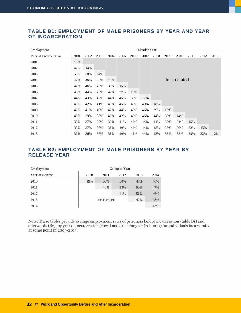
Tables B1 (B2) provide the employment rate (defined as earnings>0) for prisoners by calendar and by

year of incarceration (release). For instance, individuals who would be incarcerated in 2003 (row 3) had, in

2001 (column 1), a 50 percent employment rate; individuals incarcerated in 2007 had a 45 percent employ-

ment rate in 2005; and individuals incarcerated in 2011 had an employment rate of 36 percent in 2009 (a

recession year; in 2008 their employment rate was 44 percent). In general, employment rates vary little

across cohorts or across calendar year (with the exception of the recession, in which employment rates of

future prisoners fell by roughly ten percentage points). Similarly, upon leaving prison (Table B2), different

release cohorts fared similarly in subsequent years, with the pattern of employment largely the same one

and two years after incarceration. In other words, the poor labor market outcomes before and after incar-

ceration observed in the aggregate seem to apply generally to different cohorts and in different years.

Figure B1 shows the average employment rate of male prisoners in each state in the last full calendar

year prior to their incarceration and in the calendar year of their release for individuals who are observed

in both periods (a balanced sample). 14 Post-incarceration outcomes vary across states. A relatively high

fraction were employed in Wyoming (94 percent) and North and South Dakota (78 and 73 percent). And

employment rates are relatively high in Colorado (64 percent), Nebraska (63 percent), Iowa (63 percent),

and Idaho (63 percent). Despite high rates of employment, however, typical earnings are relatively modest

even conditional on employment, with most men earning far less than $10,000. At the other end of the

employment spectrum, far fewer individuals are employed in California (33 percent), DC (33 percent), New

York (34 percent), New Mexico (36 percent) or Ohio (36 percent).

While there are differences in employment rates across states, those differences are typically pre-exist-

ing—states with high rates of employment in their population before incarceration had relatively high rates

thereafter. The first difference in employment within states is generally small. One exception is within the

federal system, where lengthier pre-trial or pre-sentencing incarceration might mechanically have reduced

employment in the year prior to the start of the recorded sentence.

As with the national data, there is generally little evidence of an employment penalty associated with

incarceration in the comparison of pre- and post-incarceration outcomes. In almost all states, employment

(and earnings) is higher in the year of release than two years prior to incarceration. While the absence of a

decline in employment is surprising, there are several reasons why this simple comparison may understate

the effects of incarceration on employment. First, our measure of employment is generated from adminis-

trative records which generally requires that individuals receive a W2 or file a tax return. Ex-prisoners may

be encouraged or required to file a return as part of their reentry, which would boost measured employment

but not necessarily their actual employment activities. Second, we have no information on whether these

. . . 14. Compared to the figure above, the narrower timeframe, is intended to maximize the number of states and number of observa-

tions within each state available for the analysis. Because of differences in incarceration length or timing of reporting, the pre-

and post-outcomes correspond to slightly different calendar years.



individuals had prior convictions or periods of incarceration, though some surely must have. For those in-

dividuals, the pre-existing periods of incarceration may have already reduced their employment mechani-

cally (if they were incarcerated before) or because of labor market stigma (i.e., some may have already been

“marked” with a criminal record).

FIGURE B1: EMPLOYMENT BY STATE, BEFORE AND AFTER INCARCERATION

Note: This figure plots the share of prisoners with positive wage income (reported on W2 or tax forms) the calendar year prior to starting a sentence and in the calendar year of release by jurisdiction of incarceration for prisoners observed both before and after incarceration.



TABLE B1: EMPLOYMENT OF MALE PRISONERS BY YEAR AND YEAR OF INCARCERATION

Employment Calendar Year

Year of Incarceration 2001 2002 2003 2004 2005 2006 2007 2008 2009 2010 2011 2012 2013

2001 16%

2002 42% 14%

2003 50% 38% 14%

2004 49% 46% 35% 13% Incarcerated

2005 47% 46% 43% 35% 15%

2006 46% 44% 43% 42% 37% 16%

2007 44% 43% 42% 44% 45% 39% 17%

2008 43% 42% 41% 43% 45% 46% 40% 18%

2009 42% 41% 40% 42% 44% 46% 46% 39% 16%

2010 40% 39% 38% 40% 42% 45% 46% 44% 32% 14%

2011 38% 37% 37% 39% 41% 43% 44% 44% 36% 31% 15%

2012 38% 37% 36% 38% 40% 43% 44% 43% 37% 36% 32% 15%

2013 37% 36% 36% 38% 40% 42% 44% 43% 37% 38% 38% 32% 12%

TABLE B2: EMPLOYMENT OF MALE PRISONERS BY YEAR BY RELEASE YEAR

Employment Calendar Year

Year of Release 2010 2011 2012 2013 2014

2010 39% 53% 50% 47% 46%

2011 42% 53% 50% 47%

2012 41% 51% 46%

2013 Incarcerated 42% 48%

2014 43%

Note: These tables provide average employment rates of prisoners before incarceration (table B1) and afterwards (B2), by year of incarceration (rows) and calendar year (columns) for individuals incarcerated at some point in 2009-2013.



Appendix C: Incarceration by Family Income Percentile

Figure C1 shows the incarceration rate (based on the ACS overall rate for the 1980-1986 cohort that is in

prison or in jail) by parent income percentile and parent’s marital status.

The lower-than-expected incarceration rate in the bottom 3 percent of married-couple families arises

because income measured in tax records understates the real economic income of some households with

business-related expenses and resulting tax losses. We were unable to exclude those households in our

analysis. As a result, some higher-income households are effectively misclassified as low-income, reducing

the reported incarceration rate in this group.

Figure C2 shows the fraction of men in prison at age 30-34 (where the average incarceration rate in the

sample equals the BJS-reported prison incarceration rate on December 31, 2012), the fraction in prison or

in jail (as measured for the 1980-1986 birth cohort in the ACS between 2010-2014 on the day of the sample),

and the fraction in prison or in jail or a former prisoner (using the estimate from Bucknor and Barber 2016,

which suggests that for each prisoner incarcerated at age 30-34 there are about 2.78 former prisoners in

the labor force).

Figure C3 shows the share of the incarcerated population from the bottom 20 percent of the income

distribution adjusted for the share of each state’s population from the bottom 20 percent.

Despite substantial variation in the incarceration rate across states, the figure shows that the share of

the incarcerated population from the bottom 20 percent of the income distribution is very similar across

states. In just about any state, between 40 and 50 percent of the prison population grew up in families

earning less than $23,000 per year. (Alaska, Hawaii, and DC are outliers because the income distribution

in those states is high relative to the U.S. distribution—they have few low-income families.)



FIGURE C1: INCARCERATION BY FAMILY INCOME PERCENTILE AND PARENT’S MARITAL STATUS

Note: Figure shows the estimated incarceration rates of individuals born between 1980-1986 in 2012

based on the share of the 1980-1986 birth cohorts incarcerated in an adult correctional facility in the 2014

5-year American Community Survey.



FIGURE C2: FRACTION OF MEN IN PRISON, IN JAIL OR PRISON, OR IN PRISON, JAIL, OR A FORMER PRISONER, BY PARENT INCOME

Note: Figure shows the estimated share of individuals born between 1980-1986 who are in prison, in

prison or jail, or in prison, jail, or a former prisoner. “In prison” is the share observed in prison serving a

sentence of one year or greater in IRS records. “In prison or jail” is an estimate of the total incarceration

rate (in prison or in jail) based on the share of the 1980-1986 birth cohorts incarcerated in an adult cor-

rectional facility in the 2014 5-year American Community Survey. “In prison, in jail, or former prisoner”

is the sum of the ACS-estimated rate plus the number of former prisoners estimated by Bucknor and Bar-

ber 2016 and assigned in proportion to the number of individuals in prison observed in the IRS sample.



FIGURE C3: SHARE OF THE INCARCERATED POPULATION FROM THE BOTTOM 20 PERCENT OF THE INCOME DISTRIBUTION

appendix a: data - brookings.edu · we use data from reports submitted to the irs in 2014 as...

Documents