appendix-5 hydrologic study of chira river basin
TRANSCRIPT

Appendix-5 Hydrologic Study of Chira River Basin
287

288

D
InternationalCooperationAgencyJapan
PROJECT OF THE PROTECTION OF FLOOD PLAIN AND VULNERABLE RURAL POPULATION AGAINST FLOODS
IN THE REPUBLIC OF PERU
HYDROLOGY OF MAXIMUM FLOODS IN CHIRA RIVER
Appendix-5
December 2012
Yachiyo Engineering Co., Ltd.
289

Hydrology of Maximum Floods in Chira River
i
HYDROLOGY OF MAXIMUM FLOODS IN CHIRA RIVER
CONTENTS
1 INTRODUCTION 1
2 GENERAL ASPECTS 1
2.1 Location 1
2.1.1 Political Location 1
2.1.2 Geographic Location 1
2.2 Background 2
2.3 Justification of the Project 2
2.4 Objectives of the Study 2
3 PROJECT DESCRIPTION 3
3.1 Hydrographic System of Chira River 3
3.1.1 General Description of the Basin 3
3.1.2 Hydrography of the Chira River Basin 4
3.2 Climatology 5
3.2.1 Rainfall 5
3.2.2 Temperature 25
3.3 Hydrometry 26
3.4 Comments on the pluviometric and hydrometric network in the Chira
River Catchement. 30
3.4.1 On Pluviometric Stations. 30
3.4.2 On Hydrometric Stations. 30
3.4.3 Recommendations 31
4 HYDROLOGY OF MAXIMUM FLOOD 33
4.1 Preliminary Considerations 33
4.2 Hydrologic Modeling 36
4.2.1 Basin Outlining 36
4.2.2 Design Rainfall 36
4.2.3 Distribution Functions 36
4.2.3.1 Calculation of Maximum 24 hours Rainfall for Different
Return Periods 39
4.2.3.2 Map of Isohyets 40
290

Hydrology of Maximum Floods in Chira River
ii
4.2.3.3 Determination of Maximum 24-Hhours Rainfall for
Different Return Periods in the Chira River Subwatershed 43
4.2.3.4 Storm Distribution 46
4.2.4 Maximum Daily Discharge Analysis 47
4.2.5 Simulation Model, Application of HEC-HMS Software 49
4.2.5.1 Hydrological Model 49
4.2.5.2 HEC – HMS Modeling 51
4.2.5.3 Results of the Simulation, Peak Flows in the Base Poinst 54
5 REFERENCES 55
ANNEXES 56
291

Hydrology of Maximum Floods in Chira River
iii
HYDROLOGY OF MAXIMUM FLOODS IN CHIRA RIVER
LIST OF TABLES
Table Nº 3.1. Period and longitude of the available information of the Rainfall stations 6
Table Nº 3.2. Characteristics of Rainfall Stations in the Cañete River Basin and Surrounding
Basins 9
Table Nº 3.3.Results of the linear fit equation of Montero, Pananga and Santo Domingo Stations
10
Table Nº 3.4. Characteristics of Hydrometric Stations in the Chira River Basin and
Surrounding Basins 27
Table Nº 4.1. Characteristics of the Chira River Topographic Basins 36
Table Nº 4.2a. Maximum 24 Hours Raiinfall (mm) for Different Return Periods 40
Table Nº 4.2b. Maximum 24-Hours Rainfalls for Different Return Periods in each river Basin of Chira 44
Table Nº 4.3. Time Distribution of 24 Hour Rainfall. Type IA Was Used in this Simulation 46
Table Nº 4.4. Maximum Daily Discharge of station Puente Sullana and Ardilla, Chira River
(m³/s) 47
Table Nº 4.5. Maximum Discharges for each Return Period at Station Puente Sullana and
Ardilla, Chira River (m³/s) 48
Table Nº 4.6. Characteristics of the Chira River Topographic Basins 49
Table Nº 4.7. Sub-Basins of the Chira Major Basins 49
Table Nº 4.8. Maximum 24-Hour Rainfall for Sub-Basins of the Chira River Catchment 50
Table Nº 4.9. Curve Numbers for Major Basins 51
Table Nº 4.10. Adopted Base Flows for Major Basins 52
Table Nº 4.11. Summary of Peak Flows (m3/s) at the Base Points for each Return Period 54
292

Hydrology of Maximum Floods in Chira River
iv
HYDROLOGY OF MAXIMUM FLOODS IN CHIRA RIVER
LIST OF FIGURES
Figure Nº 3.1. Location Map of the Chira River Basin 4
Figure Nº 3.2. Period and longitude of the available information of the rainfall stations 7
Figure Nº 3.3. Location of the rainfall stations in Chira River basin and adjacent basins 8
Figure Nº 3.4. Monthly Histogram of Rainfall Stations considered within the Study Scope 9
Figure Nº 3.5. Annual Rainfall Trends at the Stations considered within the Study Scop 11
Figure Nº 3.6. Isohyets for Mean Monthly Rainfall in the Chira Basin, in January 12
Figure Nº 3.7. Isohyets for Mean Monthly Rainfall in the Chira Basin, in February 13
Figure Nº 3.8. Isohyets Mean Monthly Rainfall in the Chira Basin, in March 14
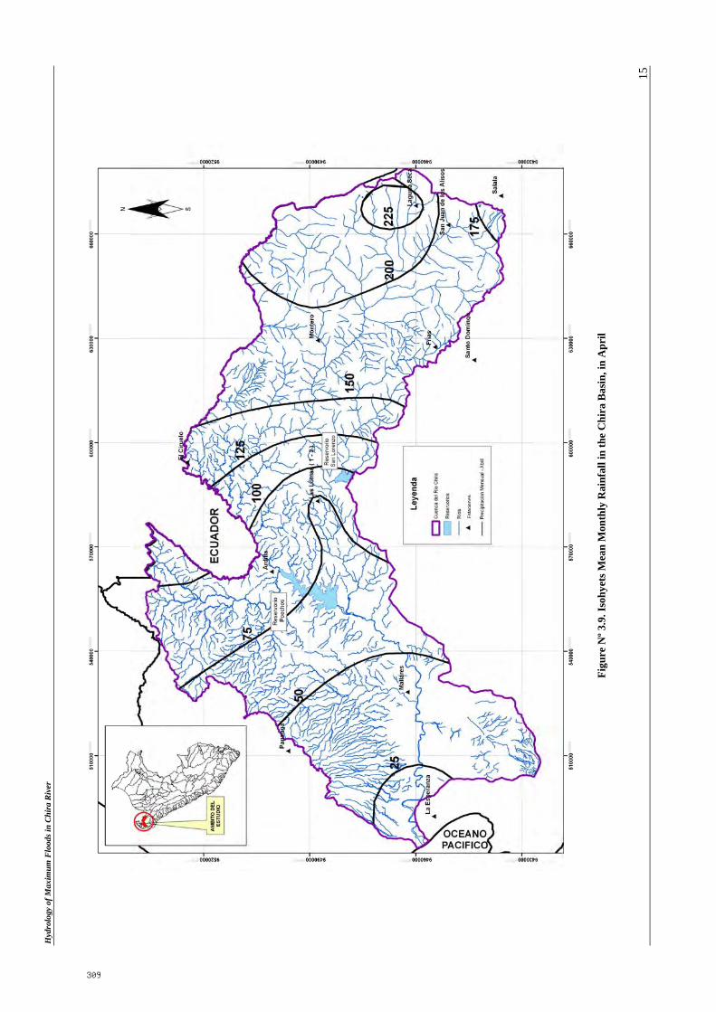
Figure Nº 3.9. Isohyets Mean Monthly Rainfall in the Chira Basin, in April 15
Figure Nº 3.10. Isohyets Mean Monthly Rainfall in the Chira Basin, in May 16
Figure Nº 3.11. Isohyets Mean Monthly Rainfall in the Chira Basin, in June 17
Figure Nº 3.12. Isohyets Mean Monthly Rainfall in the Chira Basin, in July 18
Figure Nº 3.13. Isohyets Mean Monthly Rainfall in the Chira Basin, in August 19
Figure Nº 3.14. Isohyets Mean Monthly Rainfall in the Chira Basin, in September 20
Figure Nº 3.15. Isohyets Mean Monthly Rainfall in the Chira Basin, in October 21
Figure Nº 3.16. Isohyets Mean Monthly Rainfall in the Chira Basin, in November 22
Figure Nº 3.17. Isohyets Mean Monthly Rainfall in the Chira Basin, in December 23
Figure Nº 3.18. Isohyets Annual Mean Monthly Rainfall in the Chira Basin 24
Figura Nº 3.19. Average monthly temperature for La Esperanza, Chilaco and Mallares Stations
25
Figura Nº 3.20. Average monthly temperature for La Toma Catamayo, Vilcabamba, Malacatos
and Quinara Stations 26
Figura Nº 3.21. Average monthly temperature for Zapoltillo, Macara and Sausal de Culucan
Statios 26
Figure Nº 3.22. Period and longitude of the available information of the Hydrometric Stations 27
Figure Nº 3.23. Location of the hydrometric stations in Chira River Basin and Adjacent Basins
29
Figure Nº 4.1. Relative Position of Hydrological Stations in the Study Area 35
Figure Nº 4.2a. Isohyets for the 2 - Years Return Period Maximum 24-Hours Rainfall in the
Chira Basin 40
293

Hydrology of Maximum Floods in Chira River
v
Figure Nº 4.2b. Isohyets for the 5- Years Return Period Maximum 24-Hours Rainfall in the
Chira Basin 41
Figure Nº 4.2c. Isohyets for the 10 - Years Return Period Maximum 24-Hours Rainfall in the
Chira Basin 41
Figure Nº 4.2d. Isohyets for the 25 - Years Return Period Maximum 24-Hours Rainfall in the
Chira Basin 42
Figure Nº 4.2e. Isohyets for the 50 - Years Return Period Maximum 24-Hours Rainfall in the
Chira Basin 42
Figure Nº 4.2f. Isohyets for the 100 - Years Return Period Maximum 24-Hours Rainfall in the
Chira Basin 43
Figure Nº 4.3. Chira River Subbasin 44
Figure Nº 4.4. SCS 25-Hr Rainfall Distribution for the Type I, Type IA, Type II and Type III
Rainfall Distributions. Compare to Data Registers at El Tigre Station 47
Figure Nº 4.5. Watershed considered by HEC-HMS model for the simulation. 54
294

Hydrology of Maximum Floods in Chira River
1
HYDROLOGY OF MAXIMUM FLOODS IN CHIRA RIVER
1 INTRODUCTION
In the last two extraordinary events (El Niño) occurred in 1983 and 1998, rainfall was
very intense in the study area, which resulted in the activation of a number of rivers and
streams adjacent to the Chira River, causing severe damage in populated areas,
irrigation and drainage infrastructure, agricultural lands, likewise, floods with
catastrophic damage in the areas of Sullana, Ignacio Escudero, Marcavelica,
Querecotillo, Salitral, Amopate, Colan, La Huaca and Tamarindo.
El Niño is defined as the presence of abnormally warmer waters in the west coast of
South America for a period longer than 4 consecutive months, and has its origin in the
Central Equatorial Pacific. The phenomenon is associated with abnormal conditions of
the atmospheric circulation in the Equatorial Pacific region. Abnormal conditions are
considered when the equatorial circulation scheme takes the following three
possibilities: may intensify, weaken or change direction.
This study contains a diagnosis of the problem, in order to explain the causes of the
event and guide the actions to be implemented to provide greater security to the
population, irrigation infrastructure, agricultural areas, etc. The report contains the
hydrologic analysis to allow the characterization of the event in technical terms. With
these analyses it has been possible to outline alternative structural solutions and no
structural measures.
2 GENERAL ASPECTS
2.1 Location
2.1.1 Political Location
The study area is located in the province of Sullana and Paita in the
department of Piura.
2.1.2 Geographic Location
The study area is located approximately at coordinates UTM at 482,480 y
708,883 in East Coordinates, and 9’421,040 y 9’492,030 in North
Coordinates (Zone 17).
295

Hydrology of Maximum Floods in Chira River
2
2.2 Background
As part of the project: “Protection of Rural Areas and Valleys and Flood
Vulnerable”, it requires a supporting technical document of the maximum
flooding of the Chira River, to define planning proposals hydrologic and hydraulic
Chira River system.
The occurrence of extreme events such as El Niño in the northern and southern
coast of Peru has resulted in the presence of heavy rains, rising rivers and streams
activation of contributors to the main course, such as occurred in the last two
events of 1983 and 1998. The Chira River overflowed causing flooding of
extensive crop areas and cities such as Sullana, Ignacio Escudero, Marcavelica,
Querecotillo, Salitral, Amopate, Colan, La Huaca y Tamarindo, and resulting in
damage to agriculture, road infrastructure, housing, irrigation infrastructure and
drainage. Currently there are vulnerable areas in river sections that require the
application of structural measures for flood mitigation.
An assessment of maximum floods has been made based on data from the
hydrometric station Ardillas and Puente Sullana. With the results obtained, the
hydraulic box of the will be size base to the return period chosen in specific areas
and also the design of protective structures.
2.3 Justification of the Project
Chira River allows drainage of floods from rainfalls and inflows from the
watershed.
The presence of normal hydrological events causes some damage in agricultural
areas, irrigation and drainage infrastructure, service roads and towns, therefore it
requires structural measures that allow the mitigation of extreme events up to
some degree magnitude.
2.4 Objectives of the Study
The objective of the study is to determine the maximum Chira River floods for
different return periods, to allow an appropriate measurement of the hydraulic
section of river channelization and the design of protection works, mitigating the
potential damage from extreme hydrological events.
296

Hydrology of Maximum Floods in Chira River
3
3 PROJECT DESCRIPTION
3.1 Hydrographic System of Chira River
3.1.1 General Description of the Basin
The basin of this river is geographically located between latitude 03º40'28
"and 05º07'06" of south latitude and the meridians 80º46'11 "and
79º07'52"W.
Bordered on the North River Basin Puyango, on the south by the river
basins and Huancabamba Piura, on the east by the basin and Chinchipe
Zamora (Ecuador) and on the west by the Pacific Ocean.
The Chira is an international river and its basin has a drainage area of
19.095 km2 surface until it empties into the sea, of which 7.162 km² are
within Ecuadorian territory and 11.933 km² within Peruvian territory. Its
watershed is approximately 9.500 km²
The river rises in the Cordillera Occidental of the Andes more than 3,000 m
with the name of Catamayo, and after traveling 150 km joins the river
Macara hence the name of Chira River, runs 50 km. serving as the boundary
between Peru and Ecuador to meet the continuing Alamor River in south-
west direction in Peruvian territory until it empties into the sea after having
traveled 300 km.
Its main tributaries are the rivers left bank Macara, Quiroz and Chipillico
and the right bank of the Alamor river and several streams as Hawaii,
Venados and Saman.
Figure 3.1 shows the location and area of the Chira River Basin.
297

Hydrology of Maximum Floods in Chira River
4
Figure Nº 3.1. Location Map of the Chira River Basin
3.1.2 Hydrography of the Chira River Basin
The Andes Mountains catchment areas to the country divided into two main
branches that drain their waters into the Pacific and Atlantic Oceans,
respectively, thus forming the continental divide of the waters. There is also
a third strand in the south-east of the country, consisting of a high inter-
Andean basin whose waters drain into Lake Titicaca
The basin of the Pacific or Western has an approximate area of 290.000 km²,
equivalent to 22% of the total area of the country. As a result of rainfall and
melting snow and glaciers in the upper part, 52 rivers, in some importance,
run to the Pacific Ocean predominantly towards the southwest. Chira River
is one of them, being located in the central region of this side.
The Chira river, river system belongs to the Pacific, has its source in the
Republic of Ecuador, its waterways feeding primarily to seasonal rainfall
that occur in their upper reaches. The International Basin covers an area of
19.095 km ², of which 7.162 km ² (37.51%) is in Ecuadorian territory and
11.933 km ² is located in Peruvian territory. Peruvian portion outlet of the
provinces of Paita, Talara, Piura and Ayabaca, all located in the department
of Piura
From its source and into Ecuadorian territory, the Chira River Catamayo
adopts the name, a name that kept up the border to the confluence with the
298

Hydrology of Maximum Floods in Chira River
5
river Macara with a length of about 130 km, when entering Peruvian
territory embracing the change of name of Chira River, relying on that
section with a length of 170 km., after which empties into the Pacific Ocean,
near the Old Bocana
The Chira river course, from its source to its mouth is sinuous, as in the first
section, from its source to the height of the town of Sullana, running from
northeast to southeast, then take a final direction from east to west to it
flows into the Pacific Ocean
The main tributaries of the Chira River in Peruvian territory are on the right
bank, Quebrada Honda , Peroles, La Tina, Poechos and Condor, on the left
bank rivers and Chipillico Quiroz. They are also major tributaries, the river
Pilares for its right bank and left bank Macara, which are counting on border
lines of their drainage basins in Ecuador
3.2 Climatology
3.2.1 Rainfall
The rainfall in the Chira river basin can be classified into three types: the
first, corresponds to the lower area between the contours of 0.0 and 80
meters. This stretch quite extensive, covering low rainfall of about 10-80
mm per year, concentrating on the period from January to April, and remain
dry during the remaining months of the year. Rainfall in this area are very
irregular, and appear to be closely related to the random occurrence of
severe weather caused by El Niño, they do produce very intense rainfall,
exceeding 20 times the normal values
The second type corresponds to the band located between 80 and 500 meters,
where the rains are about 100 and 600 mm. Their period of occurrence is
usually from December to May with variability characteristics less than the
first group and being in the rest of the year significantly lower in some years
even reaching zero
The third type corresponds to the band located from 500 meters to the line
of water, the upper zone due to an Amazonian rainfall regime characterized
by low variability of average annual rainfall ranging between 700 and 1.100
299

Hydrology of Maximum Floods in Chira River
6
mm., the highest recorded rainfall in the months of January to May being
the rest of the year of low intensity, but not reaching zero records. It can be
seen in this area, the incidence of severe phenomena of El Niño (random
occurrence) is almost zero.
The rainfall, as a main parameter of the runoff generation is analyzed
considering the available information of the stations located in the interior
of the Chira Basin, and in the neighboring basins.
Rainfall information is available from 13 pluviometric stations located in
the Chira River Basin and surrounding basins. These stations are operated
and maintained by the Peruvian National Service of Meteorology and
Hydrology (SENAMHI by their initials in Spanish)
Table No. 3.1, shows the list of stations included in this study with their
respective characteristics, such as code, name, and location. Historical
records of monthly total rainfall and their histograms are presented in the
Annexes. Figure Nº 3.2, shows the period and the length of the data
available from meteorological stations and Figure No. 3.3 shows the
locations in the Chira Basin and adjacent watersheds.
Table Nº 3.1. Period and longitude of the available information of the Rainfall stations
CODE STATION DEPARTAMENT LONGITUDE LATITUDE ENTITY
152202 ARDILLA (SOLANA BAJA) PIURA 80° 26'1 04° 31'1 SENAMHI
150003 EL CIRUELO PIURA 80° 09'1 04° 18'1 SENAMHI
152108 FRIAS PIURA 79° 51'1 04° 56'1 SENAMHI
230 LA ESPERANZA PIURA 81° 04'4 04° 55'55 SENAMHI
152125 LAGUNA SECA PIURA 79° 29'1 04° 53'1 SENAMHI
152104 LAS LOMAS 1 PIURA 80° 15'1 04° 38'1 SENAMHI
140 LAS LOMAS 2 PIURA 80° 15'1 04° 38'1 SENAMHI
208 MALLARES PIURA 80° 44'44 04° 51'51 SENAMHI
152144 MONTERO PIURA 79° 50'1 04° 38'1 SENAMHI
152101 PANANGA PIURA 80° 53'53 04° 33'33 SENAMHI
152135 SAN JUAN DE LOS ALISOS PIURA 79° 32'1 04° 58'1 SENAMHI
203 SALALA PIURA 79° 27'27 05° 06'6 SENAMHI
152110 SANTO DOMINGO PIURA 79° 53'1 05° 02'1 SENAMHI
300

Hydrology of Maximum Floods in Chira River
7
RIO CHIRA
1960
1961
1962
1963
1964
1965
1966
1967
1968
1969
1970
1971
1972
1973
1974
1975
1976
1977
1978
1979
1980
1981
1982
1983
1984
1985
1986
1987
1988
1989
1990
1991
1992
1993
1994
1995
1996
1997
1998
1999
2000
2001
2002
2003
2004
2005
2006
2007
2008
2009
2010
MONTERO
LAGUNA SECA
LAS LOMAS 1
LAS LOMAS 2
MALLARES
SALALA
SANTO DOMINGO
SAN JUAN DE LOS ALISOS
PANANGA
FRIAS
LA ESPERANZA
ARDILLA
EL CIRUELO
Figure Nº 3.2. Period and longitude of the available information of the rainfall stations
301

Hyd
rolo
gy o
f M
axim
um F
lood
s in
Chi
ra R
iver
8
F
igu
re N
º 3.
3. L
ocat
ion
of
the
rain
fall
sta
tion
s in
Ch
ira
Riv
er b
asin
an
d a
dja
cent
bas
ins
302

Hydrology of Maximum Floods in Chira River
9
Table N° 3.2 shows mean monthly values for the stations that have been taken
into account in the study, and Figure N° 3.4 shows the mean monthly variation
for rainfall in each station; the Annex shows the historical series for each
station, as well as the monthly and annual variation graphs for each station.
Table Nº 3.2. Characteristics of Rainfall Stations in the Chira River Basin and Surrounding Basins
Ene Feb Mar Abr May Jun Jul Ago Sep Oct Nov Dic
ARDILLA 58.0 114.2 184.1 92.4 26.8 21.5 0.0 0.4 0.1 2.6 1.5 6.9 594.1
EL CIRUELO 102.2 161.0 231.1 141.0 22.1 8.1 1.3 0.2 0.6 2.6 4.4 30.3 680.3
FRIAS 180.3 251.8 308.4 155.7 54.1 12.6 4.0 5.3 10.3 19.2 19.2 74.1 1145.9
LA ESPERANZA 14.7 17.7 28.1 17.3 12.8 7.2 0.1 0.1 0.2 0.4 0.3 3.1 100.8
LAGUNA SECA 240.2 278.2 261.0 236.0 124.1 45.0 39.7 33.8 33.8 104.7 99.2 195.5 1584.1
LAS LOMAS 1 36.8 59.7 136.9 70.6 48.9 11.0 0.1 0.1 0.5 2.5 1.5 10.1 380.0
LAS LOMAS 2 8.3 86.9 123.0 53.0 5.7 0.6 0.1 0.1 0.0 0.2 2.2 5.9 287.6
MALLARES 30.2 46.3 69.6 37.5 15.0 0.4 0.2 0.2 0.3 1.0 0.9 8.2 221.5
MONTERO 123.7 181.2 296.1 191.1 79.9 29.3 5.5 5.8 7.8 17.6 15.1 45.7 987.4
PANANGA 39.3 59.9 95.2 43.8 14.3 3.9 0.1 0.0 0.2 0.8 0.9 11.4 272.5
SAN JUAN DE LOS ALISOS 186.7 222.7 229.5 184.7 68.9 33.9 18.3 18.8 22.1 67.2 72.7 145.4 1291.0
SALALA 104.4 138.9 128.0 114.7 82.4 58.4 51.4 27.1 33.3 81.1 84.0 104.0 1029.3
SANTO DOMINGO 169.0 263.7 370.6 217.4 74.5 12.7 2.8 4.3 10.7 16.6 28.6 76.7 1233.1
ESTACIONMes
Total
0
50
100
150
200
250
300
350
400
Ene Feb Mar Abr May Jun Jul Ago Sep Oct Nov Dic
Precipitación M
ensual (mm)
Meses
ARDILLA
EL CIRUELO
FRIAS
LA ESPERANZA
LAGUNA SECA
LAS LOMAS 1
LAS LOMAS 2
MALLARES
MONTERO
PANANGA
SAN JUAN DE LOS ALISOS
SALALA
SANTO DOMINGO
Figure Nº 3.4. Monthly Histogram of Rainfall Stations considered within the Study Scope
Table N° 3.2 and Figure N° 3.4 show that heaviest rainfalls are from October
to April, and east rainfalls are from May to September. In addition, annual
rainfall in the Chira River Basin is noted to vary from 1,584 mm (Laguna Seca)
Station) to 100 mm (La Esperanza Station).
Figure N° 3.5 shows total annual rainfall variation for the stations included in
this study, with their relevant trends. Taking into account only stations Panga
303

Hydrology of Maximum Floods in Chira River
10
and Santo Domingo which are the station with mayor quantity of information ,
we established a linear equation: P = mt + b, where P is annual rainfall and t is
time in years, m and b are the variables that provide the best fit in a linear
equation. The results are presented in Table 3.3, giving the following values of
the trends:
Table Nº 3.3.Results of the linear fit equation of Montero, Pananga and Santo Domingo Stations
Estación m b R2 Montero -20.42 1256 0.072 Pananga 7.25 93.39 0.035
Santo Domingo 21.75 710.4 0.142
The value of the regression coefficients (R2) is very low. For Montero Station
would be a seasonally downward trend and for Pananga and Santo Domingo
Stations a vseasonally upward trend. R2 values indicate that the trends are not
significant and can be said that even in these stations with maximum numbers
of data there is no clear trend to increase or decrease regarding the rainfall.
Information shown in Table N° 3.2 and support from ArcGIS software have
allowed for generating monthly isohyet maps (from January to December) and
annual isohyets maps , as shown in Figures N° 3.6 – N° 3.17, and N° 3.18,
respectively.
Isohyets show that heaviest rainfalls in the basin are in March, and they vary
between 50 mm and 300 mm. The least rainfalls are in August, and they vary
between 5mm and 25 mm.
Total annual rainfall in the Chira River Basin varies between 1,400 mm and
200 mm, as shown in Figure N° 3.18.
304

Hydrology of Maximum Floods in Chira River
11
Figure Nº 3.5. Annual Rainfall Trends at the Stations considered within the Study Scop
305

Hyd
rolo
gy o
f M
axim
um F
lood
s in
Chi
ra R
iver
12
F
igur
e N
º 3.
6. I
sohy
ets
for
Mea
n M
onth
ly R
ain
fall
in t
he
Ch
ira
Bas
in, i
n J
anua
ry
306

Hyd
rolo
gy o
f M
axim
um F
lood
s in
Chi
ra R
iver
13
F
igu
re N
º 3.
7. I
soh
yets
for
Mea
n M
onth
ly R
ain
fall
in t
he
Ch
ira
Bas
in, i
n F
ebru
ary
307

Hyd
rolo
gy o
f M
axim
um F
lood
s in
Chi
ra R
iver
14
F
igur
e N
º 3.
8. I
sohy
ets
Mea
n M
onth
ly R
ainf
all i
n th
e C
hira
Bas
in, i
n M
arch
308
Hyd
rolo
gy o
f M
axim
um F
lood
s in
Chi
ra R
iver
15
F
igu
re N
º 3.
9. I
soh
yets
Mea
n M
onth
ly R
ain
fall
in t
he
Ch
ira
Bas
in, i
n A
pri
l
309

Hyd
rolo
gy o
f M
axim
um F
lood
s in
Chi
ra R
iver
16
F
igu
re N
º 3.
10. I
soh
yets
Mea
n M
onth
ly R
ain
fall
in t
he
Ch
ira
Bas
in, i
n M
ay
310

Hyd
rolo
gy o
f M
axim
um F
lood
s in
Chi
ra R
iver
17
F
igu
re N
º 3.
11. I
soh
yets
Mea
n M
onth
ly R
ain
fall
in t
he
Ch
ira
Bas
in, i
n J
un
e
311

Hyd
rolo
gy o
f M
axim
um F
lood
s in
Chi
ra R
iver
18
F
igu
re N
º 3.
12. I
soh
yets
Mea
n M
onth
ly R
ain
fall
in t
he
Ch
ira
Bas
in, i
n J
uly
312

Hyd
rolo
gy o
f M
axim
um F
lood
s in
Chi
ra R
iver
19
F
igur
e N
º 3.
13. I
sohy
ets
Mea
n M
onth
ly R
ainf
all i
n th
e C
hira
Bas
in, i
n A
ugus
t
313

Hyd
rolo
gy o
f M
axim
um F
lood
s in
Chi
ra R
iver
20
F
igu
re N
º 3.
14. I
soh
yets
Mea
n M
onth
ly R
ain
fall
in t
he
Ch
ira
Bas
in, i
n S
epte
mb
er
314

Hyd
rolo
gy o
f M
axim
um F
lood
s in
Chi
ra R
iver
21
F
igu
re N
º 3.
15. I
soh
yets
Mea
n M
onth
ly R
ain
fall
in t
he
Ch
ira
Bas
in, i
n O
ctob
er
315

Hyd
rolo
gy o
f M
axim
um F
lood
s in
Chi
ra R
iver
22
F
igur
e N
º 3.
16. I
sohy
ets
Mea
n M
onth
ly R
ainf
all i
n th
e C
hira
Bas
in, i
n N
ovem
ber
316

Hyd
rolo
gy o
f M
axim
um F
lood
s in
Chi
ra R
iver
23
F
igu
re N
º 3.
17. I
soh
yets
Mea
n M
onth
ly R
ain
fall
in t
he
Ch
ira
Bas
in, i
n D
ecem
ber
317

Hyd
rolo
gy o
f M
axim
um F
lood
s in
Chi
ra R
iver
24
F
igu
re N
º 3.
18. I
soh
yets
An
nu
al M
ean
Mon
thly
Rai
nfa
ll in
th
e C
hir
a B
asin
318

Hydrology of Maximum Floods in Chira River
25
3.2.2 Temperature
The temperature of air and its daily and seasonal variations are very important
for development of plants, being one of the main factors that directly affect the
growth rate, length of growing cycle and stages of development of perennial
plants.
The average annual temperature in the basin to the lower and middle areas
have similar values of 24 ° C, then decreases in the upper records up to 13 º C.
The maximum point values are between 13 and 15 hours, reaching 38 º C in the
lowlands (February or March) and 27 º C in the high zone.
Minima occur in the months of June through August, reaching 15 º C on the
coast, down to 8 º C during the months of June to September on top.
Figures 3.19 to 3.21 present the average monthly temperature charts for
stations in Ecuador side.
Figura Nº 3.19. Average monthly temperature for La Esperanza, Chilaco and Mallares Stations Fuente: Proyecto Binacional Catamayo - Chira
319

Hydrology of Maximum Floods in Chira River
26
Figura Nº 3.20. Average monthly temperature for La Toma Catamayo, Vilcabamba, Malacatos and Quinara Stations Fuente: Proyecto Binacional Catamayo – Chira
Figura Nº 3.21. Average monthly temperature for Zapoltillo, Macara and Sausal de Culucan Statios Fuente: Proyecto Binacional Catamayo – Chira
3.3 Hydrometry
There are 25 hydrometric stations located along the River Chira catchment and
surrounding basins. These stations are operated and maintained by the Peruvian
National Service of Meteorology and Hydrology (SENAMHI by their initials
in Spanish)
320

Hydrology of Maximum Floods in Chira River
27
Table No. 3.4, shows the list of stations included in this study with their
respective characteristics, such as code, name, and location. Historical records
of monthly total rainfall and their histograms are presented in the Annex.
Table Nº 3.4. Characteristics of Hydrometric Stations in the Chira River Basin and Surrounding Basins
START END
200302 SOLANA BAJA HLM CHIRA PIURA SULLANA LANCONES 80° 25'1 04° 31'1 112 Closed 1969-01 1975-12
200303 ZAMBA HLM CHIRA PIURA AYABACA PAIMAS 79° 54'1 04° 40'1 761 Closed
200304 LAGARTERA HLM CHIRA PIURA AYABACA SAPILLICA 80° 04'1 04° 44'1 472 Closed
200305 PUENTE SULLANA HLM CHIRA PIURA SULLANA SALITRAL 80° 41'1 04° 53'1 25 Paralyzed 1938-09 1984-12
200306 PARDO DE ZELA HLM CHIRA PIURA PIURA LAS LOMAS 80° 14'1 04° 40'1 233 Closed 1966-01 1975-02
200307 ROSITA HLM CHIRA PIURA SULLANA LANCONES 80° 30'1 04° 36'1 102 Closed
200308 CANAL MIGUEL CHECA HLM CHIRA PIURA SULLANA SULLANA 80° 31'1 04° 41'1 68 Paralyzed 1991-03 1995-07
200309 ENTRADA ARDILLA R. POECHOS HLM CHIRA PIURA SULLANA LANCONES 80° 26'1 04° 31'1 120 Paralyzed 1991-03 1997-08
200310 PUENTE INTERNACIONAL MACARA HLM CHIRA PIURA AYABACA SUYO 79° 57'1 04° 24'1 415 Paralyzed 1991-03 1997-08
200311 CANAL CHIPILLICO HLM CHIRA PIURA PIURA LAS LOMAS 80° 10'1 04° 44'1 300 Closed 1969-09 2009-11
200312 PARAJE GRANDE QUIROZ HLM CHIRA PIURA AYABACA MONTERO 79° 54'1 04° 37'1 1060 Paralyzed 1935-08 1995-07
200313 EL CIRUELO HLM CHIRA PIURA AYABACA SUYO 80° 09'1 04° 18'1 300 Paralyzed 1992-04 1992-04
200314 LOS ENCUENTROS HLM CHIRA PIURA SULLANA LANCONES 80° 17'1 04° 26'1 150 Closed 1975-11 2009-12
200316 CANAL PELADOS HLM CHIRA PIURA SULLANA SULLANA 80° 30'1 04° 41'1 100 Closed
200318 SOLANA BAJA HLM CHIRA PIURA SULLANA LANCONES 80° 25'1 04° 31'1 112 Paralyzed
200319 PUENTE SULLANA HLM CHIRA PIURA SULLANA SALITRAL 80° 41'1 04° 53'1 25 Paralyzed 1991-03 1998-01
200320 LAGARTERA HLM CHIRA PIURA AYABACA SAPILLICA 80° 04'1 04° 44'1 472 Paralyzed
200321 AYABACA HLM CHIRA PIURA AYABACA AYABACA 79° 45'1 04° 40'1 2663 Paralyzed
200322 RESERV POECHOS(VOL) HLM CHIRA PIURA SULLANA MARCAVELICA 80° 41'1 04° 31'1 333 Paralyzed
200323 RESERVORIO SAN LORENZO HLM CHIRA PIURA PIURA LAS LOMAS 80° 12'1 04° 40'1 230 Paralyzed
200324 ALAMOR HLM CHIRA PIURA SULLANA LANCONES 80° 23'56.9 04° 28'48.41 133 Operating 1997-09 2005-01
200418 CANAL YUSCAY HLM CHIRA PIURA PIURA LAS LOMAS 80° 12'1 04° 40'1 230 Paralyzed
200426 SALIDA RESERVORIO POECHOS HLM CHIRA PIURA SULLANA MARCAVELICA 80° 41'1 04° 31'1 333 Paralyzed 1991-03 1997-08
4724B080 EL CIRUELO EHA CHIRA PIURA AYABACA SUYO 80° 09'1 04° 18'1 300 Operating 2001-01 2012-06
472606OperatingA AYABACA EMA CHIRA PIURA AYABACA AYABACA 79° 43'1 04° 38'1 2757 Operating 2000-12 2011-12
Not Available
Not Available
Not Available
Not Available
Not Available
Not Available
Not Available
Not Available
Not Available
Not Available
ELEVATION CONDITION DEPARTAMENT PROVINCE DISTRICT LONGITUDE LATITUDEWORKING PERIOD
CODE STATION NAME CATEGORY* CATCHMENT
HLM = Hydrometric Station with staff gauge. It records water level manually (at 06:00, 10:00, 14:00 and 18:00 hours) to calculate daily discharges. HLG = Hydrometric Station with staff gauge and Limnigraph (floater type). It records water level manually (at 06:00, 10:00, 14:00 and 18:00 hours) to calculate daily discharges. I also it records continuously (hourly) water level data graphed in a recording paper. EHA = Automatic Hydrometric Station (hourly data of water level using sensors).
Figure Nº 3.22, shows the period and the length of the data available from the
hydrometric stations and Figure No. 3.23 shows the locations in the Chira
Basin and adjacent watersheds.
Figure Nº 3.22. Period and longitude of the available information of the Hydrometric Stations
321

Hydrology of Maximum Floods in Chira River
28
The information of the hydrometric station Ardilla will be used for calibration
of the hydrologic model to be described in item 4.2.4. This station is located
downstream of the “wet basin” of the catchment, therefore flows registered in
this station are practically the same discharge that flows to the Pacific Ocean.
322

Hyd
rolo
gy o
f M
axim
um F
lood
s in
Chi
ra R
iver
29
F
igu
re N
º 3.
23. L
ocat
ion
of
the
hyd
rom
etri
c st
atio
ns
in C
hir
a R
iver
Bas
in a
nd A
dja
cent
Bas
ins
323

Hydrology of Maximum Floods in Chira River
30
3.4 Comments on the pluviometric and hydrometric network in the
Chira River Catchement.
3.4.1 On Pluviometric Stations.
As it was stated previously the pluviometric information used in the analysis
has been provided by SENAMHI. From the 13 stations, 5 stations have data
until year 2010, 04 station has data until 1996, 02 station has data until 1995
and 01 station has data until 1987.
The stations with information previously to 2007 are not operative anymore,
although we don’t have the exact information, it is possible that the remaining
stations are currently operative. Although the information coming from stations
which have data until years previously to 1991 could be considered somewhat
old, this data have been used because their period of information are longer
than 12 years and still could be used for statistical analysis. From the 13
stations, 10 were used for the flood peak discharges analysis, the remaining
were not used due to their short period of information or the bad quality of
their data.
Rainfall records are done using manual rain gages, these devices accumulate
rain for a certain length of time after which the accumulated height of rain is
measured manually. In some cases, the readings are made once a day (at 7
am); in others, twice a day (at 7 am and 7 pm), the exact interval or readings
for the pluviometric stations used in the present analysis is not available.
3.4.2 On Hydrometric Stations.
Although these stations were operated and maintained by SENAMHI, the
hydrometric information used in the analysis was provided by The General
Directorate of Water Infrastructure (DGIH) of the Ministry of Agriculture.
From the 25 stations, 1 station has data until year 2012, 01 station has data
until 2011, 02 station have data until 2009, 01 station has data until 2005, 04
324

Hydrology of Maximum Floods in Chira River
31
station have data until 1997, 01 station has data until 1995, 01 station has data
until 1992, 01 station has data until 1984 and 02 stations have data until 1975.
For the purpose of the present study the information of hydrometric stations
Ardilla and Puente Sullana were used. Station Ardilla. The hydrometric station
Ardilla measures natural (“without project”) flows upstream the Poechos
Reservoir. The hydrometric station Puente Sullana measures flows downstream
of Poechos reservoir, these flows have lamination effect originated by the
reservoir.
In these stations water levels are measured by reading the level in a staff gages
(or rulers), lectures are transferred to a notebook and discharges are found
using an equation of the type: baHQ
Where Q is the discharge in m3/s and H is the reading in meters. These types
of stations don´t register maximum instantaneous discharge, because
recordings are not continuous and automatic, but manual. Four readings a day
are taken. Readings are taken at 6 am, 10 am, 14 pm and 18 pm. The largest
of all readings is called the daily maximum discharge, but this value is not the
maximum instantaneous daily discharge.
3.4.3 Recommendations
From a technical viewpoint, the following main recommendations can be
given:
On the Equipment
‐ In order to consider the possible differences in climates along the catchment
due to orographic effects, the number of weather and hydrometric stations
networks should be increased.
‐ In order to register the maximum instantaneous values of rainfall and
discharges, the existing manual weather and hydrometric stations should be
automated.
325

Hydrology of Maximum Floods in Chira River
32
‐ The limnigraphic equipment of the hydrometric stations should be
upgraded from the conventional paper band type to the digital band type
.
‐ Having the collected data available in real time is desirable.
‐ Study the possibility of establishing an early warning system based on
improving and increasing the number of existing hydrometric and
pluviometric stations.
‐ For complementary studies, it is advisable to acquire:
Equipment to sample sediment material.
Equipment for measuring of physical parameters for water quality
control (pH, DO, turbity and temperature)
‐ Establishment of Bench Mark (BM) for each weather and hydrometric
station using a differential GPS. This information will be useful to
replenish the station in case of its destruction by vandalism or natural
disasters.
On the Operation and Maintenance of the Equipments
‐ Weather and hydrometric stations in the study areas should be inspected
frequently.
‐ Maintenance of equipment should be in charge of qualified technicians that
are certified by the manufacturers.
‐ Periodic calibration of the equipment should be done according to the hours
of use.
On the Quality of the Measured Data
‐ Data taken manually by SENAMHI operators should be verified
independently.
326

Hydrology of Maximum Floods in Chira River
33
‐ In order to guarantee the quality of the information collected in previous
years a verification study program of the data should be done by the
government.
‐ Redundant equipment should be available in the main weather stations.
This means that duplicate equipment should be installed in selected stations
to compare readings with pattern equipment.
‐ When automatic stations are available they should operate simultaneously
with manual stations at least for one year to verify the consistency of the
data registered automatically.
It is necessary to mention that there is currently an agreement between Peru’s
National Water Authority (ANA) and SENAMHI to provide equipment to
SENAMHI weather stations financed by an external source, it is recommended
that action be taken in order to include Chira Basin in this agreement..
4 HYDROLOGY OF MAXIMUM FLOOD
4.1 Preliminary Considerations
This chapter describes the work methodology developed for the generation of flood
flows in the so-called Base Points (point of interests, Puente Sullana station and
Ardilla station) for return periods of 2, 5, 10, 25, 50, and 100 years.
The estimated maximum discharges were made from the information of maximum
24-hours rainfalls with a rainfall - runoff model, using the HEC-HMS Software. The
model was calibrated using historical records of annual maximum daily flow of the
hydrometric stations Ardilla.
Field Reconnaissance:
The field survey has included a review of the general characteristics of the Puente
Sullana hydrometric station and the base point (point of interest, where the peak
discharges will be estimated ), the major topographic features and land use in the
watershed to the study area, which has supported the definition of some parameters
to consider for the generation of flood flows.
Methodology and Procedures:
327

Hydrology of Maximum Floods in Chira River
34
Methodology and procedures developed for maximum discharge estimations are
summarized below:
● Identification and delimitation of the sub – watershed to the point of interests
(Puente Sullana Station and Ardilla Station), based on Charts at 1:100000 and / or
1:25000 scale, and satellite images.
● Selection of existing pluviometer stations in the study area and collections of
historical record of maximum 24 hour rainfall.
● Frequency analyses of maximum 24 hours rainfalls for each station and selection
of the distribution function showing the best adjustment.
● Areal rainfall calculation of the watershed to the point of interests from the
isohyetal line maps that were prepared for the 5, 10, 25, 50, and 100 – year return
periods
●
● The rainfall – runoff model generates flood flows for 5, 10, 25, 50, and 100 – year
return periods, by using the HEC – HMS software.
○ The model is calibrated based on the flow frequency law adopted for hydrometric
station Ardilla.
328

Hyd
rolo
gy o
f M
axim
um F
lood
s in
Chi
ra R
iver
35
Fig
ure
Nº
4.1.
Rel
ativ
e P
osit
ion
of H
ydro
logi
cal S
tati
ons
in t
he S
tud
y A
rea
329

Hydrology of Maximum Floods in Chira River
36
4.2 Hydrologic Modeling
4.2.1 Basin Outlining
The area of Chira River catchment until the Bridge Simón Rodriguez is 17059
km2, for modeling purposes the catchment was split in sub-basins. As this is a
bi – national basin, information was gathered from the sub – basins in the areas
relevant to the Ecuadorian side (where the Catamayo – Piura River is born) and
the Peruvian side, where the Chira River finally discharges its flows to the
Pacific Ocean.
Table 4.1 shows basins identified in a study of the Catamayo – Piura System
and their respective contribution areas.
Table Nº 4.1. Characteristics of the Chira River Topographic Basins
Sub - Basin Area (km2)
Catamayo 4184Macara 2833Quiroz 3108Alamor 1190
Chipillico 1170
Chira
C-1 878C-2 1301C-3 636C-4 921C-5 414C-6 99C-7 325
Total 17059
4.2.2 Design Rainfall
4.2.2.1 Distribution Functions
The following describes the distribution functions:
1. Distribution Normal or Gaussian
It is said that a random variable X has a normal distribution if its
density function is,
330

Hydrology of Maximum Floods in Chira River
37
To -∞ < x < ∞
Where:
f(x) = Normal density function of the variable x.
x = Independent Variable.
X = Location parameter equal to the arithmetic mean of x.
S = Scale parameter equal to the standard deviation of x.
EXP = Exponential function with base e of natural logarithms.
2. Two-Parameter Log-normal Distribution
When the logarithms, ln(x) of a variable x are normally distributed,
then we say that the distributivo of x is the probability distribution
as log–normal probability function log–normal f(x) is represented
as:
To 0<x<∞, must be x~logN( , 2)
Where:
, = Are the mean and standard deviation of the natural
logarithm of x, i.e. de ln(x), representing respectively
the scale parameter and shape parameter distribution.
3. Log–Normal Distribution of Three Parameters
Many cases the logarithm of a random variable x, the whole are not
normally distributed but subtracting a lower bound parameter xo,
before taking logarithms, we can get that is normally distributed.
The density function of the three-parameter lognormal distribution
is:
331
Hydrology of Maximum Floods in Chira River
38
To xo≤x<∞
Where:
xo = Positional parameter in the domain x
µy, = Scale parameter in the domain x.
2y = Shape parameter in the domain x
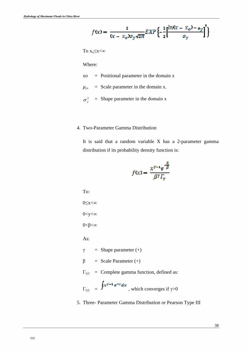
4. Two-Parameter Gamma Distribution
It is said that a random variable X has a 2-parameter gamma
distribution if its probability density function is:
To:
0≤x<∞
0<y<∞
0<β<∞
As:
γ = Shape parameter (+)
β = Scale Parameter (+)
Γ(γ) = Complete gamma function, defined as:
Γ(γ) = , which converges if γ>0
5. Three- Parameter Gamma Distribution or Pearson Type III
332

Hydrology of Maximum Floods in Chira River
39
The Log-Pearson type 3 (LP3) is a very important model in
statistical hydrology, especially after the recommendations of the
Water Resources of the United States (Water Resources Council -
WRC), to adjust the distribution Pearson Type 3 (LP3) to the
logarithms of the maximum flood. Well, the LP3 distribution is a
flexible family of three parameters can take many different forms,
therefore it is widely used in modeling annual maximum flood
series of unprocessed data.
It is said that a random variable X has a gamma distribution 3-
parameter or Pearson Type III distribution, if its probability density
function is:
To
xo≤x<∞
-∞<xo<∞
0<β<∞
0<γ<∞
4.2.2.2 Calculation of Maximum 24 hours Rainfall for Different Return Periods
Using different probability distribution functions, such as: Normal, 2
or 3 parameter Log - Normal, 2 or 3 parameter Gamma, log - Pearson
III, Gumbel, Log – Gumbel, and Widespread Extreme Values,
frequency analyses were done with the historical data of maximum 24
hours rainfall in each pluviometric station
From the information that has been generated for each distribution
function, results showing best adjustment based on the Kolgomorov –
Smirnov goodness – of - fit test will be chosen. Return periods taken
into account for this study are 2, 5, 10, 25, 50, and 100 years.
333

Hydrology of Maximum Floods in Chira River
40
Table 4.2a shows the values of the maximum 24 hours rainfall
(mm) of Mallares Station for the return periods of 10. 50, 100 and
500 years. This station has been adopted has been selected as
representative station for the purposes of the current study.
Table Nº 4.2a. Maximum 24 Hours Raiinfall (mm) for Different Return Periods
Station Elevation
(masl)
Number of
Records
Return Period (Years) Adopted
Distribution 50 100 500
Mallares 45 39 251 344 643 Log Pearson II
4.2.2.3 Map of Isohyets
With 24-hour maximum rainfall associated with the probability of occurrence
maps were generated isohyets for return period of 2, 5, 10,25, 50 and 100 years,
see Figure No. 4.2.
Figure Nº 4.2a. Isohyets for the 2 - Years Return Period Maximum 24-Hours Rainfall in the Chira Basin
334

Hydrology of Maximum Floods in Chira River
41
Figure Nº 4.2b. Isohyets for the 5- Years Return Period Maximum 24-Hours Rainfall in the Chira Basin
Figure Nº 4.2c. Isohyets for the 10 - Years Return Period Maximum 24-Hours Rainfall in the Chira Basin
335

Hydrology of Maximum Floods in Chira River
42
Figure Nº 4.2d. Isohyets for the 25 - Years Return Period Maximum 24-Hours Rainfall in the Chira Basin
Figure Nº 4.2e. Isohyets for the 50 - Years Return Period Maximum 24-Hours Rainfall in the Chira Basin
336

Hydrology of Maximum Floods in Chira River
43
Figure Nº 4.2f. Isohyets for the 100 - Years Return Period Maximum 24-Hours Rainfall in the Chira Basin
4.2.2.4 Determination of Maximum 24-Hours Rainfall for Different Return
Periods in the Chira River Subwatershed
In addition to the hydrological study of the flow in the river Chira is
required to estimate the maximum 24-hours rainfalls for different
return periods in the Chira river basins. It has been estimated from
maps shown in Figure isohyets No. 4.3.
In Figure Nº 4.3, shows the Chira river basins to which it has been
estimated maximum 24-hours rainfalls for return period and for each
subbasin. In Table Nº 4.2b are shown the values of maximum 24-
hours rainfalls for each subbasin.
337

Hydrology of Maximum Floods in Chira River
44
Figure Nº 4.3. Chira River Subbasin
Table Nº 4.2b. Maximum 24-Hours Rainfalls for Different Return Periods in each river Basin of Chira
SUBBASIN AREA [m²]
RETURN PERIOD T [YEARS]
PT_2 PT_5 PT_10 PT_25 PT_50 PT_100
1 86,237,500 18.2 56.1 85.0 133.9 180.5 237.210 75,717,500 23.1 85.2 113.2 154.1 189.2 229.011 50,042,500 22.1 97.9 124.5 160.1 188.6 219.41-1 362,845,000 17.6 45.5 70.9 115.4 159.1 213.411-1 293,953,000 22.3 103.0 128.8 161.5 186.6 212.812 89,780,000 23.2 83.7 111.7 153.0 188.7 229.212-1 166,428,000 22.1 95.5 122.5 159.3 189.5 222.413 41,395,000 22.5 88.6 116.2 155.8 189.4 227.014 152,510,000 21.7 95.7 122.9 160.3 191.1 224.9
15 137,462,000 21.2 104.1 131.0 166.5 194.6 224.515-1 145,695,000 21.5 101.4 128.1 163.2 191.1 220.816 142,630,000 21.4 91.9 122.8 167.6 205.8 248.516-1 65,240,000 22.1 107.1 132.8 164.5 188.1 212.016-2 48,107,500 21.2 102.1 130.3 168.5 199.2 232.417 57,030,000 20.3 111.4 138.7 173.8 201.0 229.317-1 33,225,000 20.9 108.4 136.4 173.2 202.2 232.917-2 86,517,500 20.4 103.2 130.6 167.6 197.3 229.218 96,660,000 20.3 120.3 147.5 181.0 205.7 230.518-1 47,667,500 20.7 120.8 148.4 182.6 207.9 233.519 43,655,000 20.3 131.1 158.7 190.9 213.5 235.119-1 61,020,000 20.2 126.1 153.3 185.7 208.9 231.62 53,395,000 24.9 63.7 94.0 142.8 187.7 240.421 56,507,500 19.6 88.7 109.7 137.7 159.9 183.52-1 506,098,000 11.7 62.5 96.3 154.0 209.5 277.121-1 58,172,500 19.9 105.0 130.3 163.2 188.7 215.421-2 182,920,000 19.6 86.1 106.7 134.5 156.8 180.5
22 25,087,500 19.6 90.9 112.4 140.9 163.6 187.522-1 61,055,000 19.7 96.8 119.8 150.0 173.7 198.7
338

Hydrology of Maximum Floods in Chira River
45
23 160,990,000 19.1 77.8 94.1 115.8 132.8 150.723-1 60,807,500 19.4 84.2 103.2 128.5 148.6 169.824 88,725,000 18.9 82.9 100.6 124.0 142.5 161.924-1 138,042,000 19.1 83.2 101.4 125.5 144.6 164.825 183,868,000 18.8 83.9 100.9 123.0 140.3 158.525-1 14,605,000 18.9 84.6 102.6 126.4 145.2 165.026 173,022,000 18.8 81.0 97.4 118.9 135.6 153.126-1 356,860,000 19.3 79.2 96.9 120.9 140.0 160.327 298,545,000 18.5 85.9 99.9 117.4 130.6 144.0
27-1 118,018,000 18.7 85.5 101.8 123.1 139.6 156.827-2 129,760,000 18.7 83.7 99.8 120.5 136.4 152.927-3 39,367,500 18.6 85.0 100.9 121.0 136.2 151.728 37,610,000 18.0 86.5 101.5 120.4 134.6 149.2
28-1 415,970,000 18.3 86.4 99.3 115.2 126.9 138.529 108,838,000 18.0 87.0 102.9 122.8 137.8 153.129-1 200,455,000 18.2 86.7 101.6 119.9 133.5 147.23 68,880,000 25.0 64.9 95.2 144.2 189.0 241.8
30 278,207,000 18.2 88.2 104.4 123.7 137.6 151.530-1 29,172,500 18.5 86.1 102.1 121.9 136.7 151.831 73,605,000 18.5 89.0 105.2 123.9 137.0 149.73-1 2,480,000 16.2 67.8 100.3 153.7 203.9 263.9
31-1 73,252,500 18.7 83.6 100.3 121.2 137.1 153.432 51,690,000 18.6 88.6 105.0 124.1 137.5 150.533 69,917,500 18.9 82.8 100.0 122.1 139.1 156.834 64,765,000 20.2 85.9 115.4 159.2 197.0 239.734-1 220,632,000 20.5 91.8 121.6 164.9 201.7 242.734-2 113,755,000 21.0 80.9 115.1 168.2 215.6 270.136 109,398,000 21.7 80.8 115.7 170.3 219.0 275.036-1 231,535,000 23.6 97.9 125.9 163.9 194.8 228.337 253,405,000 18.8 87.4 105.3 127.3 143.8 160.537-1 200,245,000 19.4 81.6 101.5 128.9 151.2 175.238 145,362,000 19.0 85.9 106.6 134.2 156.3 180.038-1 207,370,000 19.9 84.1 112.0 153.2 188.7 228.839 73,337,500 22.5 84.6 114.7 160.1 200.0 246.039-1 189,248,000 22.4 84.8 116.7 164.9 207.3 255.7
39-2 414,015,000 12.9 74.0 108.2 164.6 217.8 281.64 141,155,000 27.0 66.2 96.1 143.7 187.0 237.5
40 40,020,000 11.3 61.3 92.2 144.8 195.5 257.4
40-1 629,967,000 11.8 52.1 81.7 133.4 184.3 247.441 69,150,000 13.1 55.3 83.9 133.1 180.9 239.842 33,795,000 13.2 57.9 86.7 135.5 182.7 240.542-1 27,905,000 12.0 59.4 89.5 140.8 190.3 251.043 20,060,000 13.8 55.4 83.3 131.0 177.2 234.05 258,320,000 22.1 73.9 103.9 151.0 193.5 243.3
5-1 5,315,000 12.4 68.5 102.4 158.9 212.5 277.2
6 89,277,500 16.9 74.7 106.6 157.7 204.9 260.9
6-1 400,045,000 12.6 73.7 108.1 164.8 218.2 282.57 48,662,500 22.0 90.7 118.6 158.4 192.0 229.77-1 130,528,000 23.4 97.5 124.6 161.2 190.9 223.38 106,590,000 22.7 86.0 114.1 155.1 190.3 230.09 35,200,000 23.9 80.2 108.8 151.6 189.0 231.9
339

Hydrology of Maximum Floods in Chira River
46
4.2.2.5 Storm Distribution
Rainfall records in some stations having pluviographic stations, that is, that
they automatically measure rainfall at fixed time intervals, show that rainfall
distribution in the study area resembles a former SCS Type IA rainfall.
Table 4.3 shows rainfall distribution for the Type I, Type IA, Type II and Type
III. As seen in Figure 4.4, the highest slopes of an extreme event registered in
1998 at El Tigre Station in Tumbes, Northern Peru, resemble that of the Type I.
These events are very rare and have occurred in 1925, 1983 and 1998. No
records exist for the 1925 event, because no automatic weather stations were
available. The 1983 event destroyed the weather station.
Table Nº 4.3. Comparison of Time Distribution of the Extreme 24 Hour Rainfall Observed at El Tigre Station with Typical SCS Storm Distribution.
Time (hr) t/24 Type I Type IA Type II Type III0.00 0.000 0.000 0.000 0.000 0.0002.00 0.083 0.035 0.050 0.022 0.0204.00 0.167 0.076 0.116 0.048 0.0436.00 0.250 0.125 0.206 0.080 0.0727.00 0.292 0.156 0.268 0.098 0.0898.00 0.333 0.194 0.425 0.120 0.1158.50 0.354 0.219 0.480 0.133 0.1309.00 0.375 0.254 0.520 0.147 0.1489.50 0.396 0.303 0.550 0.163 0.1679.75 0.406 0.362 0.564 0.172 0.178
10.00 0.417 0.515 0.577 0.181 0.18910.50 0.438 0.583 0.601 0.204 0.21611.00 0.458 0.624 0.624 0.235 0.25011.50 0.479 0.654 0.645 0.283 0.29811.75 0.490 0.669 0.655 0.357 0.33912.00 0.500 0.682 0.664 0.663 0.50012.50 0.521 0.706 0.683 0.735 0.70213.00 0.542 0.727 0.701 0.772 0.75113.50 0.563 0.748 0.719 0.799 0.78514.00 0.583 0.767 0.736 0.820 0.81116.00 0.667 0.830 0.800 0.880 0.88620.00 0.833 0.926 0.906 0.952 0.95724.00 1.000 1.000 1.000 1.000 1.000
24 hr precipitation temporal distribution
340

Hydrology of Maximum Floods in Chira River
47
P/P24 Vs t/24
0.0
0.1
0.2
0.3
0.4
0.5
0.6
0.7
0.8
0.9
1.0
0.0 0.1 0.2 0.3 0.4 0.5 0.6 0.7 0.8 0.9 1.0
t/24
P/P
24
El Tigre
Tipo I
Tipo IA
Tipo II
Tipo III
Figure Nº 4.4. SCS 25-Hr Rainfall Distribution for the Type I, Type IA, Type II and Type III Rainfall Distributions. Compare to Data Registers at El Tigre Station
4.2.3 Maximum Daily Discharge Analysis
For the analysis of Maximum Daily Discharges of River Chira, the information
of the hydrometric stations Puente Sullana and Ardilla have been used. These
station have contributions areas of 14933 and 13074 km2. Figure 3.23 shows
its location in the river Chira catchment.
The Directorate General of Water Infrastructure (DGIH) of the Ministry of
Agriculture has provided information on annual maximum daily discharge of
Puente Sullana and Ardilla station whose values are shown in Table Nº 4.4
Table Nº 4.4. Maximum Daily Discharge of station Puente Sullana and Ardilla, Chira River (m³/s)
Año Puente Sullana
Ardilla
1976 2,242.00
1977 848.33 1,647.90
1978 56.12 281.10
1979 177.69 348.00
1980 57.07 438.00
1981 455.55 830.30
1982 288.18 589.10
1983 3,227.08 2,469.30
1984 1,043.00 1,663.00
1985 88.40 243.80
1986 40.00 355.60
1987 551.80 1,180.30
1988 37.70 379.50
1989 558.00 936.00
1990 45.20 253.40
1991 121.00 668.60
1992 2,355.00 3,133.50
341

Hydrology of Maximum Floods in Chira River
48
1993 1,400.00 1,654.00
1994 1,100.00 1,044.00
1995 58.00 276.10
1996 140.00 439.40
1997 925.00 1,275.80
1998 3,005.00 3,620.80
1999 1,195.20 1,927.00
2000 1,111.00 1,303.20
2001 2,252.90 2,264.80
2002 2,517.00 2,825.20
2003 169.00 371.90
2004 231.00 293.80
2005 480.00 629.00
2006 815.00 1,089.90
2007 431.10
2008 3,141.97
2009 2,387.93
These values have been analyzed with the different distribution functions
described in item 4.2..2.1. The goodness test of Kolmogrov – Smirnov shows
that the data of the hydrometric station Ardilla fits with the Log – Normal
distribution and the data of the hydrometric distribution Puente Sullana fits
with the Gumbel distribution. . The frequency analysis results are shown in
Table No 4.5.
Table Nº 4.5. Maximum Discharges for each Return Period at Station Puente Sullana and Ardilla, Chira River (m³/s)
Periodo de Retorno (Años)
Puente Sullana
Ardilla
2 890.00 895.125 1727.00 1853.4510 2276.00 2712.5325 2995.00 4070.8850 3540.00 5291.22100 4058.00 6698.22
It is necessary to mention that the Poechos Reservoir has a capacity to store
water during the wet (rainy) season to supply water for irrigation and other
purposes during the dry season. The maximum recommended operating level is
103 m.a.s.l., when the storage capacity is 490 million cubic meters (MCM), as
of December 2005. Storage capacity at the emergency spillway level (104
m.a.s.l. elevation) is 548 MCM. When the reservoir is full, the water surface is
62 km2. This datum will be used to estimate the reservoir volume during an
extreme flood flow occurrence.
342

Hydrology of Maximum Floods in Chira River
49
4.2.4 Simulation Model, Application of HEC-HMS Software
4.2.4.1 Hydrological Model
Lag Time
The Snyder formula was used to calculate the sub-basins lag time (tp):
3.075.0 CtP LLCt
Where:
Ct is a parameter related to the basin geographic characteristics.
L is the major water course length in kilometers, and
Lc is the length from the water course point that is closest to the basin’s gravity
center to the basin outlet.
Table 4.6 shows the basins identified in the Catamayo – Chira system, its
contribution areas and the parameters used for calculating lag times.
Table Nº 4.6. Characteristics of the Chira River Topographic Basins
Basin Area (km2)
L (km) Lc (km) tp (hr)
Catamayo 4184 199.33 78.29 24.45Macara 2833 155.68 73.13 22.24Quiroz 3108 201.48 83.60 25.02Alamor 1190 102.9 56.27 18.16Chipillico 1170 119.44 52.80 18.63Lower Chira 4711 119 (*) (*)
Lower Chira been sub – divided, as its sub – basins are identified as C - 1 to C
– 7, Table 4.7. shows its contribution areas and the parameters used for
calculating lag times.
Table Nº 4.7. Sub-Basins of the Chira Major Basins
Sub - Basin
Area (km2)
Length (km)
Lc (km) tp (hr)
C-1 878 34.59 15.30 8.86C-2 1301 55.31 40.95 13.70C-3 636 42.9 27.34 11.25C-4 921 47.1 19.80 10.50C-5 414 15.85 12.03 6.52C-6 99 14.78 8.31 5.72
343

Hydrology of Maximum Floods in Chira River
50
C-7 325 36.24 21.11 9.90
Maximum Rain Storm Duration
According to the "Study of the Hydrology of Peru" (Refence “d”), the average
duration of rains of Perú is 15.2 hours, due to the large size of the modeled sub-
basins, in order to be conservative a 24 hours storm duration has been assumed.
Storm Depth
The values of the maximum 24- hours rainfalls showed in Table 4.8 were
used for the calculations, these values correspond to spatial average rainfall for
the sub-basins that conform the total catchment.
Table Nº 4.8. Maximum 24-Hours Rainfall (mm) for Sub-Basins of the Chira River Catchment
Subbasin Maximum 24-Hours Rainfall for different Return Periods “Tr”
Tr= 10 years Tr= 50 years Tr= 100 years Tr= 500 years
Catamayo 99.43 250.9 344.36 643.50
Macara 99.43 250.9 344.36 643.50
Quiroz 99.43 250.9 344.36 643.50
Alamor 99.43 250.9 344.36 643.50
Chipillico 99.43 250.9 344.36 643.50
Chira
C-1 99.43 250.9 344.36 643.50
C-2 99.43 250.9 344.36 643.50
C-3 99.43 250.9 344.36 643.50
C-4 99.43 250.9 344.36 643.50
C-5 99.43 250.9 344.36 643.50 C-6 99.43 250.9 344.36 643.50 C-7 99.43 250.9 344.36 643.50
For all the subbasins the precipitation values of Mallares station have been
adopted. This asumption is conservative because, as can be seen in Table 4.2,
the areal average precipitation values estimated for the different sectors in the
catchment show lower values of precipitation than the observed in Mallares
station.
Based on item 4.2.34 a type IA distribution of the former Soil Conservation
Service storm distribution was adopted for modelling purposes.
344

Hydrology of Maximum Floods in Chira River
51
Selection of Curve Number
Because of the basin’s extension, information on soil type and land use was
gathered. Forests are predominant on the Ecuadorian side, although there are
tundras in the high areas that are basically made up of silty soils with sand and
clay contents that come close to type B soil definition. Curve numbers (CN)
were estimated with these data, by using tables from the former U.S. Soil
Conservation Service (SCS), and a weight based on the gathered information.
Table 4.9 shows the Curve Numbes for each major basin. Value obtained from
the Chira Basin will be applied for sub – basins C – 1 to C – 7, because the area
covered by the Bajo (Lower) Chira has similar characteristics.
Table Nº 4.9. Curve Numbers for Major Basins
Basin Estimated Curve Numbers
Optimized Curve
Numbers CN_1 % Area CN_2 % Area CN_II_Comp
Catamayo 55 30 65 70 62 57
Macara 55 80 65 20 57 57
Quiroz 55 30 65 70 62 58
Alamor 55 60 65 40 59 60
Chipillico 55 50 65 50 60 58
Chira 55 85 65 15 56.5 57
After calibration, compound curve numbers were optimized to the values showed in
column “Optimized Curve Numbers”. Values obtained from the Chira Basin were
applied for sub – basins C – 1 to C – 7, because the area covered by the Bajo (Lower)
Chira has similar characteristics.
4.2.4.2 HEC – HMS Modeling
The U.S. Engineer Corps’ Hydrological Engineering Center designed the
Hydrological Modeling System (HEC – HMS) computer program. This
program provides a variety of options to simulate rainfall – runoff processes,
flow routes, etc. (US Army, 2000).
HEC-HMS includes a graphic interface for the user (GUI), hydrological
analysis components, data management and storage capabilities, and facilities
to express results through graphs and reports in charts. The Guide provides all
345

Hydrology of Maximum Floods in Chira River
52
necessary means to specify the basin’s components, introduce all relevant data
of these components, and visualize the results (Reference “e” ).
Chira Basin Model.- SCS’s Curve Number method was used to estimate
losses. Snyder Unit Hydrograph method was used to transform actual rainfall
into flow. The river Chira catchemt until Puente Simón Rodriguez, of 17059
km2 , was splited in 12 sub-basins.
Table 4.10 shows the base flows adopted in the simulation to be representative
for conditions previous to the occurrence of the flood flows. This values
resulted from the available information of low flows.
Table Nº 4.10. Adopted Base Flows for Major Basins
Basin
Base Flows (m3/s)
Catamayo 46.02
Macara 31.16
Quiroz 34.19
Alamor 13.09
Chipillico 12.87
Chira
C-1 9.66
C-2 14.31
C-3 7.00
C-4 10.13
C-5 4.55
C-6 1.09
C-7 3.58
Meteorological Model.- Based on calculation under Nº 3.2 Pluviometer
Information Analysis and Frequency Law, hyetographs are introduced in the
meteorological model for a 2, 5, 10, 25, 50, and 100 – year floods, and a storm
duration of 24 hours.
Control Specifications.- Starting and ending dates are specified within the
range for the flood simulation to be carried out. Simulation results and flood
hydrograph will be submitted. In this case, starting date is February 2nd, 2010,
00:00, and end date is February 4th, 2010, 12:00 pm. Based on the
recommendation of the HEC-HMS Technical Reference Manual the minimum
computational time interval is calculated as 0.29 times the Lag Time. From
346

Hydrology of Maximum Floods in Chira River
53
Tables 4.14 and 4.15 a minimum lag time of 5.72 hours is observed, from this
value a minimum computational time of 1.66 hours is obtained. For being
conservative a computational time interval of 1 hour was used.
Calibration of the Model. Due to the fact that there was no available
information on simultaneous storm hyetographs and flood hydrographs which
would allow to calibrate model parameters for doing forecasts, the model was
calibrated based on information of estimated daily discharges.
As it was stated previously, the concept of the calibration was to adjust the
curve numbers of the sub-basings to values which produce values of peak
discharges in the point of interest Ardilla similar to the obtained for the
hydrometric station Ardilla from the statistical analysis of the maximum daily
discharges. This similitude is obtained for the different return period scenarios.
Below, Figure Nº 4.5 shows the watershed considered by HEC-HMS model for
the simulation.
347

Hydrology of Maximum Floods in Chira River
54
Figure Nº 4.5. Watershed considered by HEC-HMS model for the simulation.
4.2.4.3 Results of the Simulation, Peak Flows in the Base Poinst
Table 4.11 summarizes the peak flows for different return periods obtained with the
application of the software HEC-HMS in Chira river basin for the location of
hydrometric stations Ardilla and Puente Sullana.
Table Nº 4.11. Summary of Peak Flows (m3/s) at the Base Points for each Return Period
T [Años]
Station Ardilla
Station Puente Sullana
2 881.6 1014.3
5 1858.9 1683.7
10 2714.1 2472.1
25 4084.1 3003.6
50 5124.2 3413.7
100 6691.3 4137.6
348

Hydrology of Maximum Floods in Chira River
55
Peak flows at the base points obtained with HEC-HMS model for the return periods
of 2, 5, 10, 25, 50 and 100 years have been estimated from the maximum rainfall
generated for these return periods, adopted curve numbers and geomorphological
parameters of the basin.
As it was considered in the calibration, peak discharges obtained with HEC-HMS
model for hydrometric station Ardilla for different return periods are similar to the
correspondent maximum daily discharges showed in Table 4.5.
The detailed results of the simulations for the floods of 2, 5, 10, 25, 50 and 100 years
return period are shown in the Annexes.
5 REFERENCES
a) Association BCEOM-SOFI CONSULT S.A., “Hydrology and Meteorology
Study in the Catchments of the Pacific Littoral of Perú for Evaluation and
Forecasting of El Niño Phenomenon for Prevention and Disaster Mitigation”,
1999.
b) Chow, Maidment and Mays, “Applied Hydrology”,1994.
c) Guevara, Environmental Hydrology, 1991.
d) IILA-SENAMHI-UNI, “Study of the Hydrology of Perú”, 1982.
e) U.S. Corp of Engineers, “Manual de Referencias Técnicas del Modelo HEC-
HMS”, 2000.
349

350

Appendix-6 Hydrologic Study of Yauca River Basin
351

352

C
JapanInternationalCooperationAgency
PROJECT OF THE PROTECTION OF FLOOD PLAIN AND VULNERABLE RURAL POPULATION AGAINST FLOODS
IN THE REPUBLIC OF PERU
HYDROLOGY OF MAXIMUM FLOODS IN YAUCA RIVER
Appendix-6
December 2012
Yachiyo Engineering Co., Ltd.
353

Hydrology of Maximum Floods in Yauca River
PROJECT OF THE PROTECTION OF FLOOD PLAIN AND VULNERABLE RURAL POPULATION AGAINST FLOODS i
HYDROLOGY OF MAXIMUM FLOODS IN YAUCA RIVER
CONTENTS
I. INTRODUCTION 1
II. GENERAL ASPECTS 1
2.1 Location 1
2.1.1 Political Location 1
2.1.2 Geographic Location 1
2.2 Background 2
2.3 Justification of the Project 2
2.4 Objectives of the Study 2
III. PROJECT DESCRIPTION 3
3.1 Hydrographic System of Yauca River 3
3.1.1 General Description of the Basin 3
3.1.2 Hydrography of the Yauca River Basin 4
3.2 Climatology 5
3.2.1 Rainfall エラー! ブックマー
3.2.2 Temperature 23
IV. HYDROLOGY OF MAXIMUM FLOOD 4
4.1 Preliminary Considerations 4
4.2 Hydrology characterization, analysis of rainfall and river information 5
4.2.1 Hydrology Characterization 5
4.2.2 Maximum Rainfall in 24 Hour Analysis 5
4.2.2.1 Distribution Functions 8
4.2.2.2 Calculation of Adjustment and Return Period for
Maximum Rainfall in 24 Hours 10
4.2.2.3 Selection of Distribution Theory with better Adjustment to
the Series Record Rainfall in 24 Hours 11
4.2.2.4 Determination of Maximum Rainfall for Different Return
Periods in the Base Point 18
4.2.2.5 Determination of Maximum Rainfall for Different Return
Period in the Yauca River Subwatershed 18
4.2.3 Maximum Daily Discharge Analysis 21
4.2.4 Simulation Model, Application of HEC-HMS Software 22
4.2.4.1 Hydrological Model 22
354

Hydrology of Maximum Floods in Yauca River
PROJECT OF THE PROTECTION OF FLOOD PLAIN AND VULNERABLE RURAL POPULATION AGAINST FLOODS ii
4.2.4.2 HEC – HMS Modeling 26
4.3 Results of the Simulation, Peak Flows in the Base Point 40
ANNEXES 42
355

Hydrology of Maximum Floods in Yauca River
PROJECT OF THE PROTECTION OF FLOOD PLAIN AND VULNERABLE RURAL POPULATION AGAINST FLOODS iii
HYDROLOGY OF MAXIMUM FLOODS IN YAUCA RIVER
LIST OF TABLES
Table Nº 3.1. Characteristics of Rainfall Stations in the Yauca River Basin and Surrounding
Basins 5
Table Nº 3.2. Characteristics of Rainfall Stations in the Yauca River Basin and Surrounding
Basins 7
Table Nº 3.3.Results of the linear fit equation of Chaviñas and Carhuanillas station 8
Table Nº 3.4. Monthly maximum and minimun temperature (C°) of Yauca Station 23
Table Nº 3.5. Characteristics of Hydrometric Stations in the Yauca River Basin and
Surrounding Basins 24
Table Nº 4.1. Geomorphological Characteristics of the Basis Point Watershed (station San
Francisco Alto) 5
Table Nº 4.2. Maximum 24-hours rainfall for Stations located within the Study Scope 5
Table Nº 4.3. Determination Coefficient for each Distribution Function and for each Rainfall
Station 11
Table Nº 4.4. Maximum 24-hours rainfall of each Rainfall Station for each Return Period 11
Table Nº 4.5. Maximum Areal Rainfall in 24 Hours at the Base Point (San Francisco Alto
Station) for each Return Period 18
Table Nº 4.6. Rainfall for Different Return Periods in each river Basin of Yauca 20
Table Nº 4.7. Maximum Daily Discharge of station San Francisco Alto, Yauca River (m3/s) 21
Table Nº 4.9. Maximum Discharges for each Return Period at te Station San Francisco Alto,
Yauca River (m3/s) 22
Table Nº 4.9. Concentration and Travel Times for the Base Point (station San Francisco Alto) 22
Table Nº 4.10. Maximum Rainfall according to Dick - Peschke 24
Table Nº 4.11. Hyetograph for different Return Period 24
Table Nº 4.12. Curve Number CN Based on Land Use and Soil Hydrological 25
Table Nº 4.13. Estimated Value of Curve Number (CN) for initial calibration of HEC-HMS
Model 25
Table Nº 4.14. Generated Flood Hydrograph with HEC-HMS Model for a Return Period of 2
Years 30
Table Nº 4.15. Generated Flood Hydrograph with HEC-HMS Model for a Return Period of 5
Years 31
Table Nº 4.16. Generated Flood Hydrograph with HEC-HMS Model for a Return Period of 10
Years 34
356

Hydrology of Maximum Floods in Yauca River
PROJECT OF THE PROTECTION OF FLOOD PLAIN AND VULNERABLE RURAL POPULATION AGAINST FLOODS iv
Table Nº 4.17. Generated Flood Hydrograph with HEC-HMS Model for a Return Period of 25
Years 36
Table Nº 4.18. Generated Flood Hydrograph with HEC-HMS Model for a Return Period of 50
Years 38
Table Nº 4.19. Generated Flood Hydrograph with HEC-HMS Model for a Return Period of 100
Years 40
Table 4.20 summarizes the peak flows for different return periods obtained with the application
of the software HEC-HMS in Yauca river basin for the location of hydrometric
station San Antonio Alto. 40
Table Nº 4.21. Summary of Peak Flows at the Base Point for each Return Period 41
357

Hydrology of Maximum Floods in Yauca River
PROJECT OF THE PROTECTION OF FLOOD PLAIN AND VULNERABLE RURAL POPULATION AGAINST FLOODS v
HYDROLOGY OF MAXIMUM FLOODS IN YAUCA RIVER
LIST OF FIGURES
Figure Nº 3.1. Location Map of the Yauca River Basin 4
Figure Nº 3.2. Period and longitude of the available information of the rainfall
stations 6
Figure Nº 3.3. Location of the Rainfall Stations in Yauca River Basin and Adjacent
Basins 7
Figure Nº 3.4. Monthly Histogram of Rainfall Stations considered within the Study
Scope 7
Figure Nº 3.5. Annual Rainfall Trends at the Stations considered within the Study
Scop 9
Figure Nº 3.6. Isohyets for Mean Monthly Rainfall in the Yauca Basin, in January 10
Figure Nº 3.7. Isohyets for Mean Monthly Rainfall in the Yauca Basin, in February 11
Figure Nº 3.8. Isohyets Mean Monthly Rainfall in the Yauca Basin, in March 12
Figure Nº 3.9. Isohyets Mean Monthly Rainfall in the Yauca Basin, in April 13
Figure Nº 3.10. Isohyets Mean Monthly Rainfall in the Yauca Basin, in May 14
Figure Nº 3.11. Isohyets Mean Monthly Rainfall in the Yauca Basin, in June 15
Figure Nº 3.12. Isohyets Mean Monthly Rainfall in the Yauca Basin, in July 16
Figure Nº 3.13. Isohyets Mean Monthly Rainfall in the Yauca Basin, in August 17
Figure Nº 3.14. Isohyets Mean Monthly Rainfall in the Yauca Basin, in September 18
Figure Nº 3.15. Isohyets Mean Monthly Rainfall in the Yauca Basin, in October 19
Figure Nº 3.16. Isohyets Mean Monthly Rainfall in the Yauca Basin, in November 20
Figure Nº 3.17. Isohyets Mean Monthly Rainfall in the Yauca Basin, in December 21
Figure Nº 3.18. Isohyets Annual Mean Monthly Rainfall in the Yauca Basin 22
Figure Nº 3.19. Distribution of the monthly minimum and maximun temperature of
Yauca Station 23
Figure Nº 3.20. Period and longitude of the available information of the Hydrometric
Stations 24
358

Hydrology of Maximum Floods in Yauca River
PROJECT OF THE PROTECTION OF FLOOD PLAIN AND VULNERABLE RURAL POPULATION AGAINST FLOODS vi
Figure Nº 3.21. Location of the Hydrometric Stations Yauca River basin 8
Figure Nº 4.1. Rainfall Stations considered for HEC - HMS Software application 7
Figure Nº 4.2. Isohyets for the 2 - Years Return Period Maximum 24-Hours Rainfall
in the Yauca Basin 12
Figure Nº 4.3. Isohyets for the 5 - Years Return Period Maximum 24-Hours Rainfall
in the Yauca Basin 13
Figure Nº 4.4. Isohyets for the 10 - Years Return Period Maximum 24-Hours Rainfall
in the Yauca Basin 14
Figure Nº 4.5. Isohyets for the 25 - Years Return Period Maximum 24-Hours Rainfall
in the Yauca Basin 15
Figure Nº 4.6. Isohyets for the 50 - Years Return Period Maximum 24-Hours Rainfall
in the Yauca Basin 16
Figure Nº 4.8. Isohyets for the 100 - Years Return Period Maximum 24-Hours
Rainfall in the Yauca Basin 17
Figure Nº 4.8. Yauca River Subbasin 19
Figure Nº 4.9. Model Yauca River Basin in the HEC-HMS Software 28
Figure Nº 4.10. Hydrograph Rainfall – Runoff models of the Yauca River basin,
Return Period of 2 years 29
Figure Nº 4.11.Results Model Simulation of Rainfall – Runoff Yauca River, Return
Period of 2 years 29
Figure Nº 4.12. Hydrograph Rainfall – Runoff models of the Yauca River basin,
Return Period of 5 years 31
Figure Nº 4.13.Results Model Simulation of Rainfall – Runoff Yauca River, Return
Period of 5 years 31
Figure Nº 4.14. Hydrograph Rainfall – Runoff models of the Yauca River basin,
Return Period of 10 years 33
Figure Nº 4.15. Results Model Simulation of Rainfall – Runoff Yauca River, Return
Period of 10 years 33
Figure Nº 4.16. Hydrograph Rainfall – Runoff models of the Yauca River basin,
Return Period 25 years 35
359

Hydrology of Maximum Floods in Yauca River
PROJECT OF THE PROTECTION OF FLOOD PLAIN AND VULNERABLE RURAL POPULATION AGAINST FLOODS vii
Figure Nº 4.17. Results Model Simulation of Rainfall – Runoff Yauca River, Return
Period of 25 years 35
Figure Nº 4.18. Hydrograph Rainfall – Runoff models of the Yauca River basin,
Return Period 50 years 37
Figure Nº 4.19. Results Model Simulation of Rainfall – Runoff Yauca River, Return
Period of 50 years 37
Figure Nº 4.20. Hydrograph Rainfall – Runoff models of the Yauca River basin,
Return Period 100 years 39
Figure Nº 4.21. Results Model Simulation of Rainfall – Runoff Yauca River, Return
Period of 100 years 39
360

Hydrology of Maximum Floods in Yauca River
PROJECT OF THE PROTECTION OF FLOOD PLAIN AND VULNERABLE RURAL POPULATION AGAINST FLOODS 1
HYDROLOGY OF MAXIMUM FLOODS IN YAUCA RIVER
I. INTRODUCTION
In the last two extraordinary events (El Niño) occurred in 1983 and 1998, rainfall was very
intense in the study area, which resulted in the activation of a number of rivers and streams
adjacent to the Yauca River, causing severe damage in populated areas, irrigation and
drainage infrastructure, agricultural lands, likewise, floods with catastrophic damage in the
areas of Yauca and Jaqui.
El Niño is defined as the presence of abnormally warmer waters in the west coast of South
America for a period longer than 4 consecutive months, and has its origin in the Central
Equatorial Pacific. The phenomenon is associated with abnormal conditions of the
atmospheric circulation in the Equatorial Pacific region. Abnormal conditions are
considered when the equatorial circulation scheme takes the following three possibilities:
may intensify, weaken or change direction.
This study contains a diagnosis of the problem, in order to explain the causes of the event
and guide the actions to be implemented to provide greater security to the population,
irrigation infrastructure, agricultural areas, etc. The report contains the hydrologic analysis
to allow the characterization of the event in technical terms. With these analyses it has
been possible to outline alternative structural solutions and no structural measures.
II. GENERAL ASPECTS
2.1 Location
2.1.1 Political Location
The study area is located in the districts of Jaqui and Yauca in the province of
Caravelí, in the department of Arequipa and districts of Chavin, San Pedro,
Sancos in the province of Lucanas of department Ayacucho.
2.1.2 Geographic Location
The study area is located approximately at coordinates UTM at 546,665 y
642,595 in East Coordinates, and 8’2633,132 y 8’376,058 in North Coordinates
(Zone 18).
361

Hydrology of Maximum Floods in Yauca River
PROJECT OF THE PROTECTION OF FLOOD PLAIN AND VULNERABLE RURAL POPULATION AGAINST FLOODS 2
2.2 Background
As part of the project: “Protection of Rural Areas and Valleys and Flood Vulnerable”,
it requires a supporting technical document of the maximum flooding of the Yauca
River, to define planning proposals hydrologic and hydraulic Yauca River system.
The occurrence of extreme events such as El Niño in the northern and southern coast
of Peru has resulted in the presence of heavy rains, increased river flows and streams
activation of contributors to the main course, such as occurred in the last two events
of 1983 and 1998. The Yauca River overflowed causing flooding of extensive crop
areas and cities such Yauca and Jaqui, and resulting in damage to agriculture, road
infrastructure, housing, irrigation infrastructure and drainage. Currently there are
vulnerable areas in river sections that require the application of structural measures
for flood mitigation.
An assessment of maximum floods has been made based on data from the
hydrometric station San Francisco Alto. With the results obtained, the hydraulic box
of the will be size base to the return period chosen in specific areas and also the
design of protective structures.
2.3 Justification of the Project
Yauca River allows drainage of floods from rainfalls and inflows from the watershed.
The presence of normal hydrological events causes some damage in agricultural
areas, irrigation and drainage infrastructure, service roads and towns, therefore it
requires structural measures that allow the mitigation of extreme events up to some
degree magnitude.
2.4 Objectives of the Study
The objective of the study is to determine the maximum instant Yauca River floods
for different return periods, to allow an appropriate measurement of the hydraulic
section of river channelization and the design of protection works, mitigating the
potential damage from extreme hydrological events.
362

Hydrology of Maximum Floods in Yauca River
PROJECT OF THE PROTECTION OF FLOOD PLAIN AND VULNERABLE RURAL POPULATION AGAINST FLOODS 3
III. PROJECT DESCRIPTION
3.1 Hydrographic System of Yauca River
3.1.1 General Description of the Basin
Politically, the Yauca River basin is part of the provinces of Carvelí and
Lucanas, in the departments of Arequipa and Ayacucho respectively.
Its boundaries are: on the north by the Pampas river basins, south to Chaparra
and Chala Rivers Basin, East by the Ocoña River Basins and West by the
Pacific Ocean.
It has a total area of 4,312.29 km2 and its waters drain into the Pacific Ocean
with a tour of the main course predominantly southwesterly.
Yauca Valley, an area affected by the floods, is located in the lower basin
between latitudes 15º42’36” – 14º41’20” South and longitude 74º33’52” –
73º40’33” West. Politically it belongs to the province of Caravelí, Department
of the Arequipa.
Figure 3.1 shows the location and area of the Yauca River Basin.
363

Hydrology of Maximum Floods in Yauca River
PROJECT OF THE PROTECTION OF FLOOD PLAIN AND VULNERABLE RURAL POPULATION AGAINST FLOODS 4
Figure Nº 3.1. Location Map of the Yauca River Basin
3.1.2 Hydrography of the Yauca River Basin
The Andes Mountains catchment areas to the country divided into two main
branches that drain their waters into the Pacific and Atlantic Oceans,
respectively, thus forming the continental divide of the waters. There is also a
third strand in the south-east of the country, consisting of a high inter-Andean
basin whose waters drain into Lake Titicaca
The basin of the Pacific or Western has an approximate area of 290.000 km²,
equivalent to 22% of the total area of the country. As a result of rainfall and
melting snow and glaciers in the upper part, 52 rivers, in some importance, run
to the Pacific Ocean predominantly towards the southwest. Yauca River is one
of them, being located in the central region of this side.
Yauca River has an intermittent regimen and torrential character; its discharges
are presented in the months of January to April. The mean annual discharge of
8.38 m³/s equivalent to an average annual volume of 258.89 MMC.
364

Hydrology of Maximum Floods in Yauca River
PROJECT OF THE PROTECTION OF FLOOD PLAIN AND VULNERABLE RURAL POPULATION AGAINST FLOODS 5
The supply of water to the valley of Yauca is regulated, due to intermittent
regimen Yauca River which has downloads only between the months of
January to April, during the remainder of the river dries up considerably.
During this period, the dry season, water is discharged regulation of the gap
between the months of August through December.
3.2 Climatology
3.2.1 Rainfall
The rainfall, as a main parameter of the runoff generation is analyzed
considering the available information of the stations located in the interior of
the Yauca Basin, and in the neighboring Pampas, Chaparra, Chala and Ocoña.
Rainfall information is available from 7 pluviometric stations located in the
vicinity of the study area; these are located in the Yauca River Basin and
surrounding basins. These stations are operated and maintained by the Peruvian
National Service of Meteorology and Hydrology (SENAMHI by their initials
in Spanish)
Table No. 3.1, shows the list of stations included in this study with their
respective characteristics, such as code, name, and location. Historical records
of monthly total rainfall and their histograms are presented in the Annex.
Figure Nº 3.2, shows the period and the length of the data available from
meteorological stations and Figure No. 3.3 shows the locations in the Yauca
Basin and adjacent watersheds.
Table Nº 3.1. Characteristics of Rainfall Stations in the Yauca River Basin and Surrounding Basins
CODE STATION DEPARTAMENT LONGITUDE LATITUDE ENTITY
157216 TARCO AREQUIPA 73°45'1 15°18'1 SENAMHI
740 SANCOS AYACUCHO 73° 57'1 15° 04'1 SENAMHI
743 CORACORA2 AYACUCHO 73° 47'1 15° 01'1 SENAMHI
154 CORA CORA AYACUCHO 73° 47'47 15° 01'1 SENAMHI
742 CHAVIÑA AYACUCHO 73° 50'1 14° 59'1 SENAMHI
157220 CARHUANILLAS AYACUCHO 73° 44'1 15° 08'1 SENAMHI
732 YAUCA AREQUIPA 74° 31'1 15° 40'1 SENAMHI
365

Hydrology of Maximum Floods in Yauca River
PROJECT OF THE PROTECTION OF FLOOD PLAIN AND VULNERABLE RURAL POPULATION AGAINST FLOODS 6
RIO YAUCA
1960
1961
1962
1963
1964
1965
1966
1967
1968
1969
1970
1971
1972
1973
1974
1975
1976
1977
1978
1979
1980
1981
1982
1983
1984
1985
1986
1987
1988
1989
1990
1991
1992
1993
1994
1995
1996
1997
1998
1999
2000
2001
2002
2003
2004
2005
2006
2007
2008
2009
2010
CORACORA
CHAVIÑA
CARHUANILLAS
YAUCA
TARCO
SANCOS
CORACORA2
Figure Nº 3.2. Period and longitude of the available information of the rainfall stations
366

Hydrology of Maximum Floods in Yauca River
PROJECT OF THE PROTECTION OF FLOOD PLAIN AND VULNERABLE RURAL POPULATION AGAINST FLOODS 7
Figure Nº 3.3. Location of the Rainfall Stations in Yauca River Basin and Adjacent Basins
Table N° 3.2 shows mean monthly values for the stations that have been taken
into account in the study, and Figure N° 3.4 shows the mean monthly variation
for rainfall in each station; the Annex shows the historical series for each
station, as well as the monthly and annual variation graphs for each station.
Table Nº 3.2. Characteristics of Rainfall Stations in the Yauca River Basin and Surrounding Basins
ESTACION Mes
TotalEne Feb Mar Abr May Jun Jul Ago Sep Oct Nov Dic
TARCO 116.76 85.09 121.13 26.66 0.00 0.00 0.00 0.00 1.36 7.07 15.80 29.27 403.13
SANCOS 131.88 133.65 105.28 4.96 0.39 0.00 0.41 0.00 0.63 2.38 1.72 10.46 391.75
CORACORA2 102.06 118.34 104.25 19.40 2.08 1.09 1.76 2.54 6.13 7.09 10.78 34.86 410.36
CORA CORA 176.24 163.85 301.90 155.00 216.45 234.55 137.45 68.05 127.76 199.38 274.25 188.46 2,243.33
CHAVIÑA 115.10 142.42 161.44 32.21 5.12 0.87 0.93 3.86 10.45 11.79 10.76 45.59 540.54
CARHUANILLAS 116.28 150.78 145.02 37.01 1.26 0.00 0.64 2.03 3.57 9.73 13.91 32.15 512.38
YAUCA 0.00 0.00 0.02 0.00 0.00 0.00 0.00 0.00 0.00 0.00 0.00 0.00 0.00
0
50
100
150
200
250
300
350
Ene Feb Mar Abr May Jun Jul Ago Sep Oct Nov Dic
MESES
PR
EC
IPIT
AC
ION
ME
NS
UA
L [
mm
]
TARCO
SANCOS
CORACORA2
CORA CORA
CHAVIÑA
CARHUANILLAS
YAUCA
Figure Nº 3.4. Monthly Histogram of Rainfall Stations considered within the Study Scope
Table 3.2 and Figure No. 3.4 show that the information of Coracora station
does not have the same behavior against the other stations, so we discard the
information in this station. Also, Table N° 3.2 and Figure N° 3.4 show that
heaviest rainfalls are from November to April, and east rainfalls are from May
to September. In addition, annual rainfall in the YaucaRiver Basin is noted to
vary from 540.54 mm (Chaviña Station) to 0.00 mm (Yauca Station).
367

Hydrology of Maximum Floods in Yauca River
PROJECT OF THE PROTECTION OF FLOOD PLAIN AND VULNERABLE RURAL POPULATION AGAINST FLOODS 8
Figure N° 3.5 shows total annual rainfall variation for the stations included in
this study, with their relevant trends. Taking into account only stations
Chaviñas and Carhuanillas which are the station that have the most amount of
data , we established a linear equation: P = mt + b, where P is annual rainfall
and t is time in years, m and b are the variables that provide the best fit in a
linear equation. The results are presented in Table 3.3, giving the following
values of the trends:
Table Nº 3.3.Results of the linear fit equation of Chaviñas and Carhuanillas station
Station m b R2 Chaviñas 10.12 435.9 0.081 Carhuanillas -20.25 813.2 0.198
The value of the regression coefficients (R2) is very low. For Chaviñas Station
would be a seasonally weak upward trend and for Carhuanillas Station a
seasonally weak downward trend. R2 values indicate that the trends are not
significant very and can be said that even in these stations with maximum
numbers of data there is no clear trend to increase or decrease regarding the
rainfall.
Information shown in Table N° 3.2 and support from ArcGIS software have
allowed for generating monthly isohyet maps (from January to December) and
annual isohyets maps , as shown in Figures N° 3.6 – N° 3.17, and N° 3.18,
respectively.
The annual rainfall in the river Yauca basin varies in ranges from 500 mm to
100 mm, as shown in Figure No. 3.18.
368

Hydrology of Maximum Floods in Yauca River
PROJECT OF THE PROTECTION OF FLOOD PLAIN AND VULNERABLE RURAL POPULATION AGAINST FLOODS 9
PRECIPITACION TOTAL ‐ ANUAL (mm), ESTACION SANCOS
0
200
400
600
800
1000
1200
1400
1600
1800
2000
1963
1964
1965
1966
1967
1968
1969
1970
1971
1972
1973
1974
1975
1976
1977
1978
1979
1980
AÑOS
PRECIPITACION (mm)
PRECIPITACION TOTAL ‐ ANUAL (mm), ESTACION CORACORA2
0
100
200
300
400
500
600
700
800
1963
1965
1967
1969
1971
1973
1975
1977
1979
1981
1983
1985
1987
1989
1991
1993
1995
1997
1999
2001
2003
2005
2007
2009
AÑOS
PRECIPITACION (mm)
PRECIPITACION TOTAL ‐ ANUAL (mm), ESTACION CHAVIÑA
0
200
400
600
800
1000
1200
1963
1964
1965
1966
1967
1968
1969
1970
1971
1972
1973
1974
1975
1976
1977
1978
1979
1980
1981
1982
1983
AÑOS
PRECIPITACION (mm)
PRECIPITACION TOTAL ‐ ANUAL (mm), ESTACION CARHUANILLAS
0
200
400
600
800
1000
1200
1400
1965
1966
1967
1968
1969
1970
1971
1972
1973
1974
1975
1976
1977
1978
1979
1980
1981
1982
1983
1984
1985
1986
1987
AÑOS
PRECIPITACION (mm)
PRECIPITACION TOTAL ‐ ANUAL (mm), ESTACION YAUCA
0
0
0
0
0
1
1
1
1
1
1
1963
1965
1967
1969
1971
1973
1975
1977
1979
1981
1983
1985
1987
1989
1991
AÑOS
PRECIPITACION (mm)
Figure Nº 3.5. Annual Rainfall Trends at the Stations considered within the Study Scop
369
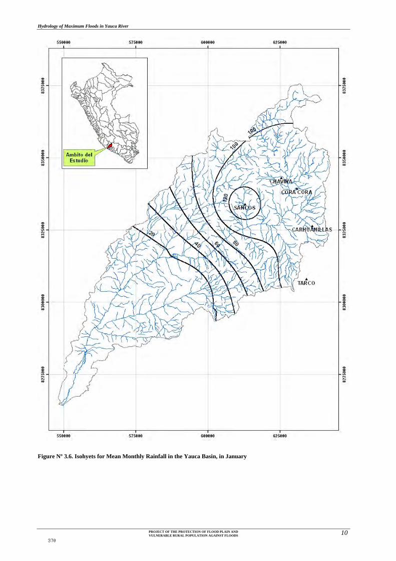
Hydrology of Maximum Floods in Yauca River
PROJECT OF THE PROTECTION OF FLOOD PLAIN AND VULNERABLE RURAL POPULATION AGAINST FLOODS 10
Figure Nº 3.6. Isohyets for Mean Monthly Rainfall in the Yauca Basin, in January
370

Hydrology of Maximum Floods in Yauca River
PROJECT OF THE PROTECTION OF FLOOD PLAIN AND VULNERABLE RURAL POPULATION AGAINST FLOODS 11
Figure Nº 3.7. Isohyets for Mean Monthly Rainfall in the Yauca Basin, in February
371

Hydrology of Maximum Floods in Yauca River
PROJECT OF THE PROTECTION OF FLOOD PLAIN AND VULNERABLE RURAL POPULATION AGAINST FLOODS 12
Figure Nº 3.8. Isohyets Mean Monthly Rainfall in the Yauca Basin, in March
372

Hydrology of Maximum Floods in Yauca River
PROJECT OF THE PROTECTION OF FLOOD PLAIN AND VULNERABLE RURAL POPULATION AGAINST FLOODS 13
Figure Nº 3.9. Isohyets Mean Monthly Rainfall in the Yauca Basin, in April
373

Hydrology of Maximum Floods in Yauca River
PROJECT OF THE PROTECTION OF FLOOD PLAIN AND VULNERABLE RURAL POPULATION AGAINST FLOODS 14
Figure Nº 3.10. Isohyets Mean Monthly Rainfall in the Yauca Basin, in May
374

Hydrology of Maximum Floods in Yauca River
PROJECT OF THE PROTECTION OF FLOOD PLAIN AND VULNERABLE RURAL POPULATION AGAINST FLOODS 15
Figure Nº 3.11. Isohyets Mean Monthly Rainfall in the Yauca Basin, in June
375

Hydrology of Maximum Floods in Yauca River
PROJECT OF THE PROTECTION OF FLOOD PLAIN AND VULNERABLE RURAL POPULATION AGAINST FLOODS 16
Figure Nº 3.12. Isohyets Mean Monthly Rainfall in the Yauca Basin, in July
376

Hydrology of Maximum Floods in Yauca River
PROJECT OF THE PROTECTION OF FLOOD PLAIN AND VULNERABLE RURAL POPULATION AGAINST FLOODS 17
Figure Nº 3.13. Isohyets Mean Monthly Rainfall in the Yauca Basin, in August
377

Hydrology of Maximum Floods in Yauca River
PROJECT OF THE PROTECTION OF FLOOD PLAIN AND VULNERABLE RURAL POPULATION AGAINST FLOODS 18
Figure Nº 3.14. Isohyets Mean Monthly Rainfall in the Yauca Basin, in September
378

Hydrology of Maximum Floods in Yauca River
PROJECT OF THE PROTECTION OF FLOOD PLAIN AND VULNERABLE RURAL POPULATION AGAINST FLOODS 19
Figure Nº 3.15. Isohyets Mean Monthly Rainfall in the Yauca Basin, in October
379

Hydrology of Maximum Floods in Yauca River
PROJECT OF THE PROTECTION OF FLOOD PLAIN AND VULNERABLE RURAL POPULATION AGAINST FLOODS 20
Figure Nº 3.16. Isohyets Mean Monthly Rainfall in the Yauca Basin, in November
380

Hydrology of Maximum Floods in Yauca River
PROJECT OF THE PROTECTION OF FLOOD PLAIN AND VULNERABLE RURAL POPULATION AGAINST FLOODS 21
Figure Nº 3.17. Isohyets Mean Monthly Rainfall in the Yauca Basin, in December
381

Hydrology of Maximum Floods in Yauca River
PROJECT OF THE PROTECTION OF FLOOD PLAIN AND VULNERABLE RURAL POPULATION AGAINST FLOODS 22
Figure Nº 3.18. Isohyets Annual Mean Monthly Rainfall in the Yauca Basin
382

Hydrology of Maximum Floods in Yauca River
PROJECT OF THE PROTECTION OF FLOOD PLAIN AND VULNERABLE RURAL POPULATION AGAINST FLOODS 23
3.2.2 Temperature
The temperature of air and its daily and seasonal variations are very important
for development of plants, being one of the main factors that directly affect the
growth rate, length of growing cycle and stages of development of perennial
plants.
The temperature is the factor most linked to their altitudinal variations. In the
basin, it has been seen that varies from semi-warm (19 °C approximately) in
the area of coast to the frigid type (5 °C approximately) in the area of puna,
falls between these extremes a number thermal variations that characterize each
of the altitudinal appreciated in the watershed.
The existing meteorological network, only have reliable statistical data on
temperature at 4 stations. Three are located in Coracora, Chavin and Sancos
respectively (Sierra or mountain side), and one is in Yauca (coast side). Table
No. 3.4 presents the maximum and minimum monthly temperature and Figure
N ° 3.19 shows the monthly temperature varied from the station Yauca
Table Nº 3.4. Monthly maximum and minimun temperature (C°) of Yauca Station
TEMPERATURA Mes
PromedioEne Feb Mar Abr May Jun Jul Ago Sep Oct Nov Dic
Maxima 27.40 27.90 27.60 26.00 24.00 21.90 20.30 20.10 20.70 22.10 23.90 25.80 23.98
Minima 18.30 17.80 17.70 16.30 13.60 11.30 10.90 11.00 12.20 12.80 14.40 16.40 14.39
Fuente: Asignación de Agua en Bloque en el Valle Yauca, ATDR Acari-Yauca-Puquio, 2006
Figure Nº 3.19. Distribution of the monthly minimum and maximun temperature of Yauca Station Fuente: Asignación de Agua en Bloque en el Valle Yauca, ATDR Acari-Yauca-Puquio, 2006
383

Hydrology of Maximum Floods in Yauca River
PROJECT OF THE PROTECTION OF FLOOD PLAIN AND VULNERABLE RURAL POPULATION AGAINST FLOODS 24
3.3 Hydrometry
There are 2 hydrometric stations located along the River Yauca catchment and
surrounding basins. These stations are operated and maintained by the Peruvian
National Service of Meteorology and Hydrology (SENAMHI by their initials
in Spanish).
Table No. 3.5, shows the list of stations included in this study with their
respective characteristics, such as code, name, and location. Historical records
of monthly total rainfall and their histograms are presented in the Annex.
Table Nº 3.5. Characteristics of Hydrometric Stations in the Yauca River Basin and Surrounding Basins
START END
204002 PUENTE JAQUI HLG YAUCA AREQUIPA CARAVELI JAQUI 74° 27'1 15° 29'1 247 Closed 1951-09 1986-09
213801 LA PALMA HLG YAUCA AYACUCHO LUCANAS SANCOS 74° 19'0 15° 18'0 618 Paralyzed
----- SAN FRANCISCO ALTO HLG YAUCA AREQUIPA CARAVELI SAN FRANCISCO ALTO 74º 25' 43 15º27'84 385 Operating 1961 2010
WORKING PERIODCODE STATION NAME CATEGORY* CATCHMENT DEPARTAMENT PROVINCE DISTRICT LONGITUDE LATITUDE ELEVATION CONDITION
Not Available
HLG = Hydrometric Station with staff gauge and Limnigraph (floater type). It records water level manually (at 06:00, 10:00, 14:00 and 18:00
hours) to calculate daily discharges. I also it records continuously (hourly) water level data graphed in a recording paper.
Figure Nº 3.20, shows the period and the length of the data available from the
hydrometric stations and Figure No. 3.21 shows the locations in the Yauca
Basin and adjacent watersheds.
RIVER YAUCA
1951
1952
1953
1954
1955
1956
1957
1958
1959
1960
1961
1962
1963
1964
1965
1966
1967
1968
1969
1970
1971
1972
1973
1974
1975
1976
1977
1978
1979
1980
1981
1982
1983
1984
1985
1986
1987
1988
1989
1990
1991
1992
1993
1994
1995
1996
1997
1998
1999
2000
2001
2002
2003
2004
2005
2006
2007
2008
PUENTE JAQUI
LA PALMA
SAN FRANCISCO ALTONOT AVAILABLE
Figure Nº 3.20. Period and longitude of the available information of the Hydrometric Stations
The information of the hydrometric station San Francisco Alto will be used for
calibration of the hydrologic model to be described in item 4.2.4. This station
is located downstream of the “wet basin” of the catchment, therefore flows
registered in this station are practically the same discharge that flows to the
Pacific Ocean.
384

Hyd
rolo
gy o
f M
axim
um F
lood
s in
Yau
ca R
iver
PR
OJE
CT
OF
TH
E P
RO
TE
CT
ION
OF
FL
OO
D P
LA
IN A
ND
V
UL
NE
RA
BL
E R
UR
AL
PO
PU
LA
TIO
N A
GA
INS
T F
LO
OD
S
8
F
igu
re N
º 3.
21. L
ocat
ion
of
the
Hyd
rom
etri
c S
tati
ons
Yau
ca R
iver
bas
in
385

Hydrology of Maximum Floods in Yauca River
PROJECT OF THE PROTECTION OF FLOOD PLAIN AND VULNERABLE RURAL POPULATION AGAINST FLOODS 1
3.4 Comments on the hydrologic and meteorologic network in the Yauca River Catchement.
3.4.1 On Pluviometric Stations.
As it was stated previously the pluviometric information used in the analysis has
been provided by SENAMHI. From the 7 stations, only one station has data until
year 2010, 1 station has data until 2005, 1 station has data until 1993, 1 station
has data until 1987, 1 station has data until 1982, 1 station has data until 1980, and
1 station has data until 1972. The stations with information previously to 1992 are
not operative anymore; only Cora Cora 2 station is operative.
Rainfall records are done using manual rain gages, these devices accumulate rain
for a certain length of time after which the accumulated height of rain is measured
manually. In some cases, the readings are made once a day (at 7 am); in others,
twice a day (at 7 am and 7 pm), the exact interval or readings for the pluviometric
stations used in the present analysis is not available.
3.4.2 On Hydrometric Stations.
Although these stations were operated and maintained by SENAMHI, the
hydrometric information used in the analysis was provided by The General
Directorate of Water Infrastructure (DGIH) of the Ministry of Agriculture.
From the 3 stations, 1 stations has data until year 2008, 01 station has data until
1986, the data from the remaining two stations ware not available.
For the purpose of the present study the information of hydrometric station San
Francisco Alto was used. In this station water levels are measured by reading
the level in a staff gage (or ruler), lectures are transferred to a notebook and
discharges are found using an equation of the type:
baHQ
Where Q is the discharge in m3/s and H is the reading in meters. These types of
stations don´t register maximum instantaneous discharge, because recordings are
not continuous and automatic, but manual. Four readings a day are taken.

Hydrology of Maximum Floods in Yauca River
PROJECT OF THE PROTECTION OF FLOOD PLAIN AND VULNERABLE RURAL POPULATION AGAINST FLOODS 2
Readings are taken at 6 am, 10 am, 14 pm and 18 pm. The largest of all readings
is called the daily maximum discharge, but this value is not the maximum
instantaneous daily discharge.
3.4.3 Recommendations
From a technical viewpoint, the following main recommendations can be
given:
On the Equipment
‐ In order to consider the possible differences in climates along the catchment
due to orographic effects, the number of weather and hydrometric stations
networks should be increased.
‐ In order to register the maximum instantaneous values of rainfall and
discharges, the existing manual weather and hydrometric stations should be
automated.
‐ The limnigraphic equipment of the hydrometric stations should be
upgraded from the conventional paper band type to the digital band type
.
‐ Having the collected data available in real time is desirable.
‐ Study the possibility of establishing an early warning system based on
improving and increasing the number of existing hydrometric and
pluviometric stations.
‐ For complementary studies, it is advisable to acquire:
Equipment to sample sediment material.
Equipment for measuring of physical parameters for water quality
control (pH, DO, turbity and temperature)
‐ Establishment of Bench Mark (BM) for each weather and hydrometric
station using a differential GPS. This information will be useful to
387

Hydrology of Maximum Floods in Yauca River
PROJECT OF THE PROTECTION OF FLOOD PLAIN AND VULNERABLE RURAL POPULATION AGAINST FLOODS 3
replenish the station in case of its destruction by vandalism or natural
disasters.
On the Operation and Maintenance of the Equipments
‐ Weather and hydrometric stations in the study areas should be inspected
frequently.
‐ Maintenance of equipment should be in charge of qualified technicians that
are certified by the manufacturers.
‐ Periodic calibration of the equipment should be done according to the hours
of use.
On the Quality of the Measured Data
‐ Data taken manually by SENAMHI operators should be verified
independently.
‐ In order to guarantee the quality of the information collected in previous
years a verification study program of the data should be done by the
government.
‐ Redundant equipment should be available in the main weather stations.
This means that duplicate equipment should be installed in selected stations
to compare readings with pattern equipment.
‐ When automatic stations are available they should operate simultaneously
with manual stations at least for one year to verify the consistency of the
data registered automatically.
It is necessary to mention that there is currently an agreement between Peru’s
National Water Authority (ANA) and SENAMHI to provide equipment to
SENAMHI weather stations financed by an external source, it is recommended that
action be taken in order to include Chincha Basin in this agreement.
388

Hydrology of Maximum Floods in Yauca River
PROJECT OF THE PROTECTION OF FLOOD PLAIN AND VULNERABLE RURAL POPULATION AGAINST FLOODS 4
IV. HYDROLOGY OF MAXIMUM FLOOD
4.1 Preliminary Considerations
This chapter describes the work methodology developed for the generation of flood
flows in the so-called Base Point (point of interest, San Francisco Alto station) for
return periods of 2, 5, 10, 25, 50, and 100 years.
The estimated maximum discharge was made from the information of rainfall up to
24 hours with a rainfall - runoff models, using the HEC-HMS Software. The model
was calibrated using historical records of annual maximum daily flow of the San
Francisco Alto station.
Field Reconnaissance:
The field survey has included a review of the general characteristics of the San
Francisco Alto hydrometric station and the base point (point of interest, where the
peak discharges will be estimated), the major topographic features and land use in
the watershed to the study area, which has supported the definition of some
parameters to consider for the generation of flood flows.
Methodology and Procedures:
Methodology and procedures developed for maximum discharge estimations are
summarized below:
● Identification and delimitation of the sub – watershed to the point of interest (San
Francisco Alto Station), based on Charts at 1:100000 and / or 1:25000 scale, and
satellite images.
● Selection of existing pluviometer stations in the study area and collections of
historical record of maximum24 – hours rainfall.
● Frequency analyses of maximum 24 – hour rainfalls for each station and selection
of the distribution function showing the best adjustment.
● Areal rainfall calculation of the watershed to the interest point from the isohyetal
line maps that were prepared for the 2, 5, 10, 25, 50, and 100 – year return periods.
389

Hydrology of Maximum Floods in Yauca River
PROJECT OF THE PROTECTION OF FLOOD PLAIN AND VULNERABLE RURAL POPULATION AGAINST FLOODS 5
● Establishment of the maximum rainfall for a storm’s duration no less than the
time of concentration (time in which the entire basin inputs to the discharge)
through the Dick and Peschke model.
● The rainfall – runoff model generates flood flows for 2, 5, 10, 25, 50, and 100 –
year return periods, by using the HEC – HMS software, and modeled the basin
based on the following steps:
○ Based on the daily maximum annual flow historical series, the flow frequency
law is calculated by means of statistical methods.
○ Calibration of the rainfall – runoff model based on the flow frequency law.
4.2 Hydrology characterization, analysis of rainfall and river information
4.2.1 Hydrology Characterization
The geomorphological characteristics of the basis point watershed (station San
Francisco Alto) shown in Table Nº 4.1.
Table Nº 4.1. Geomorphological Characteristics of the Basis Point Watershed (station San Francisco Alto) Caracteristic Value
Catchment Area (km2) 3,190.000
Major water course length (km) 136.000
Maximum Altitude (msnm) 4,540.000
Minimum Slope (msnm) 447.000
Average Slope (m/m) 0.030
4.2.2 Maximum 24-Hours Rainfall Analysis
Table N° 3.1 and Figure N° 3.3 show the stations located within the study
scope (the Yauca River Basin and adjacent basins). Maximum 24 – hour
annual rainfall in these stations are shown in Table N° 4.2; daily and maximum
24- hour information is shown in the Annex.
From the Information in Table N° 4.2 and Figure N° 3.3,we conclude that the
stations are located throughout the area of study .
Table Nº 4.2. Maximum 24-hours rainfall for Stations located within the Study Scope
Year Pluviometric Stations
390

Hydrology of Maximum Floods in Yauca River
PROJECT OF THE PROTECTION OF FLOOD PLAIN AND VULNERABLE RURAL POPULATION AGAINST FLOODS 6
TARCO SANCOS CORACORA CHAVIÑA CARHUANILLAS YAUCA
1960
1961
1962
1963
1964 25.00 24.50 0.00
1965 25.20 26.50 0.00
1966 17.10 21.00 30.60 0.00
1967 44.80 53.40 35.70 45.00 0.00
1968 30.00 49.30 31.00 35.50
1969 25.00 32.00 24.00 32.90 0.00
1970 40.10 28.50 29.70 0.00
1971 15.60 20.50 30.00 41.40 49.50 0.00
1972 10.90 57.50 27.00 57.30 32.00 0.00
1973 15.00 38.01 32.00 46.40 20.00 0.00
1974 28.00 30.00 34.00 30.00
1975 61.90 28.00 30.90 53.00 0.00
1976 44.80 44.40 37.00 0.00
1977 45.20 36.50 20.00 32.00
1978 33.00 15.40 79.50
1979 13.80 20.80 22.80 13.10 0.00
1980 19.90 21.70 29.70 23.00
1981 27.40 34.00 30.50 0.00
1982 25.40 12.10
1983 13.50
1984
1985 15.10
1986 19.10
1987 34.80
1988
1989
1990
1991 30.20
1992
1993 30.40
1994 30.00
1995 28.00
1996
1997 30.70
1998
1999
2000 28.00
2001 31.60
2002 29.10
2003 29.00
2004
2005 157.80
2006 59.50
2007
2008
2009
2010
Figure N° 4.1 shows the stations included in the following analyses, as applied
to HEC – HMS software.
391

Hydrology of Maximum Floods in Yauca River
PROJECT OF THE PROTECTION OF FLOOD PLAIN AND VULNERABLE RURAL POPULATION AGAINST FLOODS 7
Figure Nº 4.1. Rainfall Stations considered for HEC - HMS Software application
Each maximum annual rainfall series for all five (5) selected rainfall stations
will be adjusted to a specific distribution type. In this sense, most common
distribution functions are described, as applied to the extreme event
hydrological studies.
392

Hydrology of Maximum Floods in Yauca River
PROJECT OF THE PROTECTION OF FLOOD PLAIN AND VULNERABLE RURAL POPULATION AGAINST FLOODS 8
4.2.2.1 Distribution Functions
The following describes the distribution functions:
1. Distribution Normal or Gaussiana
It is said that a random variable X has a normal distribution if its
density function is,
To -∞ < x < ∞
Where:
f(x) = Normal density function of the variable x.
x = Independent Variable.
X = Location parameter equal to the arithmetic mean of x.
S = Scale parameter equal to the standard deviation of x.
EXP = Exponential function with base e of natural logarithms.
2. Two-Parameter Log-normal Distribution
When the logarithms, ln(x) of a variable x are normally distributed,
then we say that the distributivo of x is the probability distribution
as log–normal probability function log–normal f(x) is represented
as:
To 0<x<∞, must be x~logN( , 2)
Where:
, = Are the mean and standard deviation of the natural
logarithm of x, i.e. de ln(x), representing respectively
the scale parameter and shape parameter distribution.
393

Hydrology of Maximum Floods in Yauca River
PROJECT OF THE PROTECTION OF FLOOD PLAIN AND VULNERABLE RURAL POPULATION AGAINST FLOODS 9
3. Log–Normal Distribution of Three Parameters
Many cases the logarithm of a random variable x, the whole are not
normally distributed but subtracting a lower bound parameter xo,
before taking logarithms, we can get that is normally distributed.
The density function of the three-parameter lognormal distribution
is:
To xo≤x<∞
Where:
xo = Positional parameter in the domain x
µy, = Scale parameter in the domain x.
2y = Shape parameter in the domain x
4. Two-Parameter Gamma Distribution
It is said that a random variable X has a 2-parameter gamma
distribution if its probability density function is:
To:
0≤x<∞
0<y<∞
0<β<∞
As:
γ = Shape parameter (+)
β = Scale Parameter (+)
394

Hydrology of Maximum Floods in Yauca River
PROJECT OF THE PROTECTION OF FLOOD PLAIN AND VULNERABLE RURAL POPULATION AGAINST FLOODS 10
Γ(γ) = Complete gamma function, defined as:
Γ(γ) = , which converges if γ>0
5. Three- Parameter Gamma Distribution or Pearson Type III
The Log-Pearson type 3 (LP3) is a very important model in
statistical hydrology, especially after the recommendations of the
Water Resources of the United States (Water Resources Council -
WRC), to adjust the distribution Pearson Type 3 (LP3) to the
logarithms of the maximum flood. Well, the LP3 distribution is a
flexible family of three parameters can take many different forms,
therefore it is widely used in modeling annual maximum flood
series of unprocessed data.
It is said that a random variable X has a gamma distribution 3-
parameter or Pearson Type III distribution, if its probability density
function is:
To
xo≤x<∞
-∞<xo<∞
0<β<∞
0<γ<∞
4.2.2.2 Calculation of Adjustment and Return Period for Maximum Rainfall
in 24 Hours
Frequency of maximum 24-hours rainfall in each station (see Table N°
4.2) was analyzed by using the “CHAC” Extreme Hydrological
Events Software (developed by CEDEX - Spain),. This software
calculates Maximum 24 – hour rainfall for different return periods,
based on the probability distribution functions, such as: Normal, 2 or 3
395

Hydrology of Maximum Floods in Yauca River
PROJECT OF THE PROTECTION OF FLOOD PLAIN AND VULNERABLE RURAL POPULATION AGAINST FLOODS 11
parameter Log - Normal, 2 or 3 parameter Gamma, log - Pearson III,
Gumbel, Log – Gumbel, and Widespread Extreme Values.
From the information that has been generated for each distribution
function, results showing best adjustment based on the Kolgomorov –
Smirnov goodness – of - fit test will be chosen. Return periods taken
into account for this study are 2, 5, 10, 25, 50, and 100 years.
4.2.2.3 Selection of Distribution Theory with better Adjustment to the Series
Record Rainfall in 24 Hours
According to the analysis with the software CHAC note that the data
fit the distribution function of Generalized Extreme Value (GEV) as
the distribution coefficient, see Table No 4.3. The values for each
return period are shown in Table No 4.4.
Table Nº 4.3. Determination Coefficient for each Distribution Function and for each Rainfall Station
Station Determination Coeffcient for Each Distribution Function
Log Pearson III GEV SQRT Gumbel Log-Normal
Acnococha 0.94 0.95 0.93 0.93 0.90
Choclococha 0.94 0.95 0.93 0.90 0.91
Cocas 0.94 0.95 0.90 0.93 0.93
Hacienda Bernales 0.89 0.93 0.88 0.90 0.90
Huamani 0.94 0.95 0.94 0.92 0.89
Table Nº 4.4. Maximum 24-hours rainfall of each Rainfall Station for each Return Period
NAME OF STATION RETURN PERIOD T [YEARS]
PT_2 PT_5 PT_10 PT_25 PT_50 PT_100 PT_200
CARHUANILLAS 26.0 42.0 54.0 70.0 84.0 98.0 114.0
CHAVIÑA 32.0 42.0 48.0 54.0 59.0 62.0 66.0
CORA CORA 28.0 36.0 41.0 46.0 49.0 52.0 54.0
SANCOS 34.0 48.0 57.0 67.0 74.0 80.0 86.0
TARCO 20.0 32.0 41.0 54.0 65.0 77.0 91.0
Information shown in Table N° 4.4 and the Interpolate to Raster’s IDW
(Inverse Distance Weighted) tool in the ArcGIS Spatial Analyst module
have allowed to generate spatial rainfall distribution for each return
period.
To generate maps isohyets tool has been used Contour Surface Analysis
of Spatial Analyst module of ArcGIS Software, whose results are
shown in Figures N° 4.2 to 4.7.
396

Hydrology of Maximum Floods in Yauca River
PROJECT OF THE PROTECTION OF FLOOD PLAIN AND VULNERABLE RURAL POPULATION AGAINST FLOODS 12
Based on the isohyets maps for each return period, maximum rainfall
for the basin area has been estimated, as established for the Base Point
(San Francisco Station). Methodology and results are described under
4.2.2.4.
Figure Nº 4.2. Isohyets for the 2 - Years Return Period Maximum 24-Hours Rainfall in the Yauca Basin
397
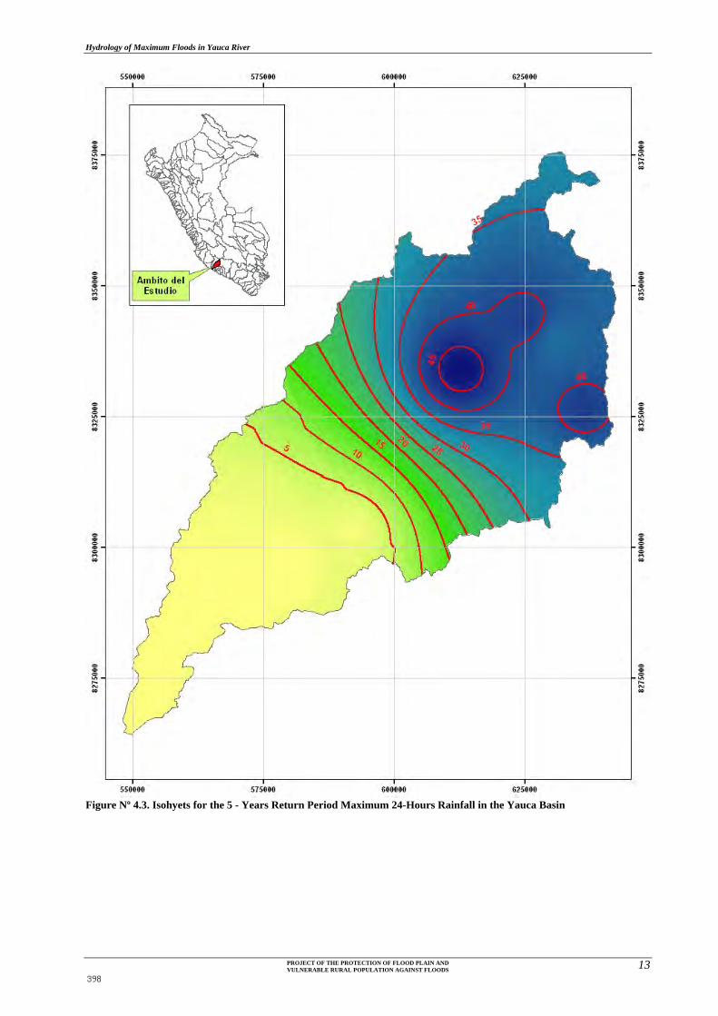
Hydrology of Maximum Floods in Yauca River
PROJECT OF THE PROTECTION OF FLOOD PLAIN AND VULNERABLE RURAL POPULATION AGAINST FLOODS 13
Figure Nº 4.3. Isohyets for the 5 - Years Return Period Maximum 24-Hours Rainfall in the Yauca Basin
398

Hydrology of Maximum Floods in Yauca River
PROJECT OF THE PROTECTION OF FLOOD PLAIN AND VULNERABLE RURAL POPULATION AGAINST FLOODS 14
Figure Nº 4.4. Isohyets for the 10 - Years Return Period Maximum 24-Hours Rainfall in the Yauca Basin
399

Hydrology of Maximum Floods in Yauca River
PROJECT OF THE PROTECTION OF FLOOD PLAIN AND VULNERABLE RURAL POPULATION AGAINST FLOODS 15
Figure Nº 4.5. Isohyets for the 25 - Years Return Period Maximum 24-Hours Rainfall in the Yauca Basin
400

Hydrology of Maximum Floods in Yauca River
PROJECT OF THE PROTECTION OF FLOOD PLAIN AND VULNERABLE RURAL POPULATION AGAINST FLOODS 16
Figure Nº 4.6. Isohyets for the 50 - Years Return Period Maximum 24-Hours Rainfall in the Yauca Basin
401

Hydrology of Maximum Floods in Yauca River
PROJECT OF THE PROTECTION OF FLOOD PLAIN AND VULNERABLE RURAL POPULATION AGAINST FLOODS 17
Figure Nº 4.8. Isohyets for the 100 - Years Return Period Maximum 24-Hours Rainfall in the Yauca Basin
402

Hydrology of Maximum Floods in Yauca River
PROJECT OF THE PROTECTION OF FLOOD PLAIN AND VULNERABLE RURAL POPULATION AGAINST FLOODS 18
4.2.2.4 Determination of Maximum 24-Hours Rainfall for Different Return
Periods in the Base Point
Isohyet maps for each return period (2, 5, 10, 25, 50, and 100 years)
and the Zonal Statistics tool from the ArcGIS software’s Spatial
Analyst module have allowed for calculating maximum 24 – hour
areal rainfall at the base point (San Francisco Alto Station) for each
return period. Results are shown in Table N° 4.5.
Table Nº 4.5. Maximum Areal Rainfall in 24 Hours at the Base Point (San Francisco Alto Station) for each Return Period
Return Period
“T” [Years]
Maximum Areal
24 Hours Rainfall
[mm]
2 23.00
5 28.00
10 33.00
25 39.00
50 45.00
100 50.00
4.2.2.5 Determination of Maximum 24- HoursRainfall for Different Return
Period in the Yauca River Subwatershed
In addition to the hydrological study of the flow in the river Yauca is
required to estimate the maximum rainfall for different return periods
in the Yauca river basins. It has been estimated from isohyet maps
shown in Figures N° 4.2. to N° 4.7 and the methodology that is briefly
described under 4.2.2.4.
Figure Nº 4.8 shows the Yauca river subbasins to which it has been
estimated maximum rainfall for each return period and for each
subbasin. Table Nº 4.6 shows the values of rainfall for each subbasin.
403

Hydrology of Maximum Floods in Yauca River
PROJECT OF THE PROTECTION OF FLOOD PLAIN AND VULNERABLE RURAL POPULATION AGAINST FLOODS 19
Figure Nº 4.8. Yauca River Subbasin
404

Hydrology of Maximum Floods in Yauca River
PROJECT OF THE PROTECTION OF FLOOD PLAIN AND VULNERABLE RURAL POPULATION AGAINST FLOODS 20
Table Nº 4.6. Rainfall for Different Return Periods in each river Basin of Yauca
SUBCUENCA AREA [m²]
PERIODO DE RETORNO T [AÑOS]
PT_2 PT_5 PT_10 PT_25 PT_50 PT_100
1 61,284,500 1.6 2.6 3.4 5.2 6.9 9.410 55,272,700 30.3 42.3 50.1 58.9 65.4 71.0
11 30,944,400 30.5 40.8 47.2 54.0 59.3 63.31-1 118,833,000 0.1 0.2 0.2 0.4 0.5 0.811-1 93,098,900 28.6 39.1 45.9 53.6 59.5 64.812 26,390,500 30.7 40.8 47.1 53.7 58.9 62.61-2 143,100,000 0.3 0.8 1.3 2.7 4.0 6.312-1 1,383,670 30.5 40.0 45.9 51.8 56.4 59.613 137,225,000 28.9 38.7 44.9 51.5 56.7 60.813-1 32,052,500 29.7 39.1 45.0 51.0 55.6 59.114 192,151,000 25.6 35.0 41.1 48.1 53.5 58.315 50,349,700 27.4 37.0 43.2 50.0 55.4 59.916 16,954,800 28.6 38.1 44.1 50.5 55.4 59.516-1 568,670 28.5 37.7 43.5 49.6 54.1 57.917 32,660,500 27.7 37.3 43.5 50.3 55.5 60.018 48,910,200 27.2 36.9 43.3 50.4 55.9 60.9
18-1 43,177,700 28.1 36.9 42.5 48.3 52.4 56.119 78,792,400 26.9 38.2 45.9 55.4 62.9 70.3
19-1 25,910,700 27.9 37.3 43.4 50.1 54.9 59.5
2 386,631,000 12.2 17.4 20.9 25.4 29.1 33.1
20 98,980,600 25.6 40.4 51.3 65.8 78.3 90.821 34,183,400 20.6 32.2 40.7 52.8 62.9 73.72-1 55,336,800 1.9 3.2 4.2 6.2 8.2 11.221-1 112,005,000 24.1 36.2 44.8 56.0 65.3 74.722 50,395,500 19.8 30.4 38.1 48.9 57.9 67.42-2 104,677,000 11.8 16.9 20.4 25.1 28.9 33.123 73,007,700 19.2 28.8 35.5 44.6 52.2 60.1
23-1 60,112,300 25.1 36.3 43.9 53.4 61.0 68.324 77,914,200 22.3 32.3 39.2 47.8 54.7 61.525 68,850,300 6.8 10.4 13.0 17.3 21.3 26.125-1 77,030,500 0.8 1.9 2.8 5.4 8.3 12.425-2 213,313,000 1.1 2.1 2.9 4.8 6.8 9.825-3 91,892,800 0.3 0.6 0.8 2.1 2.7 4.726 120,127,000 12.2 18.2 22.5 28.5 33.7 39.426-1 208,752,000 12.5 18.2 22.1 27.5 32.2 37.227 61,181,900 5.8 9.0 11.3 15.3 19.1 23.7
27-1 93,813,100 0.8 1.8 2.7 5.1 7.8 11.628 29,264,100 0.9 1.7 2.4 4.3 6.0 8.829 31,413,300 0.9 1.6 2.1 3.7 4.9 7.13 75,074,500 23.9 33.2 39.2 46.3 51.7 56.7
30 11,649,000 0.4 0.8 1.0 2.3 2.9 4.9
30-1 23,518,800 0.2 0.4 0.6 1.7 2.1 3.931 32,366,600 0.3 0.6 0.8 1.7 2.2 3.63-1 78,873,900 24.4 34.2 40.6 48.1 53.7 58.931-1 85,790,400 0.2 0.3 0.4 0.9 1.1 1.831-2 36,947,100 0.1 0.2 0.3 1.0 1.2 2.1
31-3 134,614,000 0.2 0.3 0.4 0.7 0.8 1.2
4 104,276,000 27.2 37.3 43.8 51.1 56.7 61.55 90,318,700 28.7 40.1 47.4 55.6 61.8 67.1
6 22,411,600 29.0 40.8 48.5 57.3 63.6 69.36-1 89,267,400 14.4 20.5 24.6 30.0 34.3 38.87 56,625,200 13.8 19.7 23.8 29.1 33.5 38.17-1 111,631,000 16.4 23.4 28.2 34.3 39.2 44.2
8 52,246,200 28.9 40.8 48.5 57.4 63.8 69.6
8-1 812,255 28.1 39.7 47.3 56.2 62.8 68.89 71,716,500 32.4 45.7 54.2 63.7 70.5 76.4
9-1 6,557,560 29.3 41.4 49.3 58.3 65.1 71.1
405
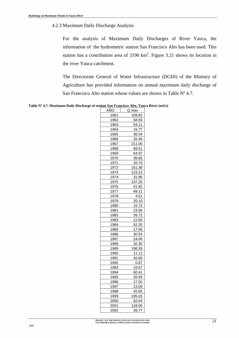
Hydrology of Maximum Floods in Yauca River
PROJECT OF THE PROTECTION OF FLOOD PLAIN AND VULNERABLE RURAL POPULATION AGAINST FLOODS 21
4.2.3 Maximum Daily Discharge Analysis
For the analysis of Maximum Daily Discharges of River Yauca, the
information of the hydrometric station San Francisco Alto has been used. This
station has a contribution area of 3190 km2. Figure 3.21 shows its location in
the river Yauca catchment.
The Directorate General of Water Infrastructure (DGIH) of the Ministry of
Agriculture has provided information on annual maximum daily discharge of
San Francisco Alto station whose values are shown in Table Nº 4.7.
Table Nº 4.7. Maximum Daily Discharge of station San Francisco Alto, Yauca River (m3/s) AÑO Q max
1961 109.821962 58.931963 54.111964 15.771965 36.541966 26.491967 211.061968 68.511969 64.971970 36.651971 20.701972 151.381973 123.131974 31.961975 137.201976 41.821977 69.111978 4.511979 20.101980 15.721981 23.561982 26.721983 12.601984 52.201985 17.651986 30.541987 24.061988 32.301989 198.391990 11.121991 42.601992 0.671993 19.571994 60.411995 20.931996 17.501997 13.091998 45.651999 195.032000 62.642001 118.062002 39.77
406

Hydrology of Maximum Floods in Yauca River
PROJECT OF THE PROTECTION OF FLOOD PLAIN AND VULNERABLE RURAL POPULATION AGAINST FLOODS 22
2003 45.812004 33.462005 6.612006 78.542007 50.142008 42.28
These values have been analyzed with different distribution functions
described in item 4.2.1.1. and evidence of Kolmogrov - Smirnok best fits the
Log - Pearson 3 parameters. The results are shown in Table No 4.8.
Table Nº 4.9. Maximum Discharges for each Return Period at te Station San Francisco Alto, Yauca River (m3/s) Return Period
(Years) Maximum
Daily Discharge
(m3/s) 2 38.395 79.2110 119.9025 187.0350 263.41100 354.38
4.2.4 Simulation Model, Application of HEC-HMS Software
4.2.4.1 Hydrological Model
Time of Concentration and Travel Time
USDA/SCS Unit Synthetic Hydrograph model was used to calculate
the following parameters:
Concentration time (Tc) with the Bransby-Williams formula
Tc = 0,95*(L3/H)0,385
Where:
L = The largest raindrop route at the main river bed (km)
H = Head (m)
Tc = Concentration time (Hr)
Travel time (Tv) = 0,6*Tc
Table Nº 4.9. Concentration and Travel Times for the Base Point (station San Francisco Alto) L = 136.00 Km
407

Hydrology of Maximum Floods in Yauca River
PROJECT OF THE PROTECTION OF FLOOD PLAIN AND VULNERABLE RURAL POPULATION AGAINST FLOODS 23
H = 4,093.00 Mts
Tc = 11.25 Hrs
Tv = 6.75 Hrs
Maximum Rain Storm Duration
Because the information of storms given by SENAMHI was provided
in a daily basis, the information about the duration of the storm was
not known. For this reason, based on the information of duration of
storms in Perú, mentioned in the "Study of the Hydrology of Peru"
(Refence “d”), a duration of 10 hours was adopted.
This value is lower than the time of concentration of 11.25 hours
calculated in the previous item, it indicates that the peak values to be
estimated in the hydrometric station San Francisco Alto won´t
correspond to the simultaneous contribution of runoff of the whole
catchement of the river Yauca until the hydrometric station San
Francisco Alto.
Storm Depth
The storm depths for a duration of 10 hours were calculated using the
equation of Dick and Peschke (Reference “c”) which allows to
estimate the maximum rainfall for a given storm duration from a 24-
hour maximum rainfall. The values of 24 hour maximum rainfall
showed in Table 4.5 were used for the calculations, these values
correspond to an spatial average rainfall for the catchment until
hydrometric station San Francisco Alto.
Dick and Peschke equation :
Pd = Pd24*(Tc/1440)0,25
Where:
Pd = Maximum rainfall for a duration d
408

Hydrology of Maximum Floods in Yauca River
PROJECT OF THE PROTECTION OF FLOOD PLAIN AND VULNERABLE RURAL POPULATION AGAINST FLOODS 24
Pd24= 24 – hour maximum rainfall
Tc= Concentration time (minutes)
Table Nº 4.10. Maximum Rainfall according to Dick - Peschke
T [Años]
Pp Areal Max24 Horas
[mm]
Pp Max, [mm]
2 23.00 18.92
5 28.00 22.50
10 33.00 26.51
25 39.00 31.33
50 45.00 36.15
100 50.00 40.17
The maximum daily rainfall for return periods of 2, 5, 10, 25, 50, and
100 – year are 23, 28, 33, 39, 45 and 50 mm, respectively, and for a
duration of 10 hour storm are 19, 23, 27, 31, 36 and 40 mm,
respectively.
In the study cited above (Study of the Hydrology Service of Peru,
1982), for a frequency interval 1 hour storm duration for up to 10
hours, has the intensity distribution, see Table Nº 4.11.
Table Nº 4.11. Hyetograph for different Return Period Return Period [Years]
Hour Total Rainfall1 2 3 4 5 6 7 8 9 10
2 1 2 2 4 3 2 2 2 1 1 18.92
5 1 2 3 4 3 3 2 2 1 1 23.04
10 1 2 4 5 4 3 3 2 2 1 27.15
25 2 3 4 6 4 4 3 3 2 1 32.09
50 2 3 5 7 5 4 4 3 2 1 37.03
100 2 4 5 8 6 5 4 3 2 2 41.14
Selection of Curve Number
When maximum flood records are available at local or regional
hydrometric stations, curve numbers can be calculated from
calibration.
Typically, selection of the curve number (CN) is done based on the
hydrologicsoil group and the land use description.
Group A: Deep sand, deep wind – deposited soils, aggregate silts.
Group B: Shallow wind – deposited soils, sandy marl.
409

Hydrology of Maximum Floods in Yauca River
PROJECT OF THE PROTECTION OF FLOOD PLAIN AND VULNERABLE RURAL POPULATION AGAINST FLOODS 25
Group C: Clayey marls, sandy shallow marls, soils with high clay
contents.
Group D: Expansive soils, highly plastic clays.
Table Nº 4.12 shows the CN as a function of hydrologic soil group
and land uses.
Table Nº 4.12. Curve Number CN Based on Land Use and Soil Hydrological
Based on land uses, and adopting the hydrologic soil group C for the
whole catchment, an initial areal averaged curve number of 85.5 was
adopted for Yauca Basin. In Table 4.13 the estimated percentages of
land use with their respective values of curves of number for river
Yauca are shown.
Table Nº 4.13. Estimated Value of Curve Number (CN) for initial calibration of HEC-HMS Model Uso del Suelo % CN
Tierras Cultivadas
Sin Tratamiento de Consevacion 40.00 88.0
Con Tratamiento de Consevacion 5.00 78.0
Tierras Cultivadas
Condicones Pobres 30.00 86.0
Condicones Optimas 5.00 74.0
Praderas 4.00 71.0
Bosques Troncos delgados 5.00 77.0
Cubierta Buena 1.00 70.0
Area comerciales 1.00 94.0
Zonas Industriales 1.00 91.0
Zonas residensiales 5.00 81.0
410

Hydrology of Maximum Floods in Yauca River
PROJECT OF THE PROTECTION OF FLOOD PLAIN AND VULNERABLE RURAL POPULATION AGAINST FLOODS 26
Calles y carreteras
Pavimentadas con cunetas 1.00 98.0
Grava 1.00 89.0
Tierra 2.00 87.0
Curva de Numero de la Cuenca 101.00 85.5
After the process of calibration of the model HEC-HMS, this value
was adjusted to 74.
4.2.4.2 HEC – HMS Modeling
The U.S. Engineer Corps’ Hydrological Engineering Center designed
the Hydrological Modeling System (HEC – HMS) computer program.
This program provides a variety of options to simulate rainfall –
runoff processes, flow routes, etc. (US Army, 2000).
HEC-HMS includes a graphic interface for the user (GUI),
hydrological analysis components, data management and storage
capabilities, and facilities to express results through graphs and reports
in charts. The Guide provides all necessary means to specify the
basin’s components, introduce all relevant data of these components,
and visualize the results (Reference “e” ).
San Francisco Alto Basin Model.- SCS’s Curve Number method was
used to estimate losses. SCS’s Unit Hydrograph method was used to
transform actual rainfall into flow. In addition, the 2981 km2 basin
area is taken into account as basic information. Due to the small
averages discharges generally observed in river Yauca it was assumed
that there was no base flow previous to the occurrence of the flood
flows.
Meteorological Model.- Based on calculation under Nº 3.2
Pluviometer Information Analysis and Frequency Law, hyetographs
are introduced inthe meterological model for a 2, 5, 10, 25, 50, and
100 – year floods, and a storm duration of 10 hours.
Control Specifications.- Starting and ending dates are specified for
the flood simulation to be carried out. Simulation results and flood
411

Hydrology of Maximum Floods in Yauca River
PROJECT OF THE PROTECTION OF FLOOD PLAIN AND VULNERABLE RURAL POPULATION AGAINST FLOODS 27
hydrograph will be submitted. In this case, starting date is February
2nd, 2010, 00:00, and end date is February 4th, 2010, 12:00 pm.
Based on the recommendation of the HEC-HMS Technical Reference
Manual the minimum computational time interval is calculated as 0.29
times the Lag Time. Aproximating the Lag Time as 0.6 times the
Concentration Time, a lag time of 6.75 hours and a minimum
computational time of 1.95 hours are obtained. For the simulation a
computational time interval of 1 hour was used.
Calibration of the Model. Due to the fact that there was no available
information on simultaneous storm hyetographs and flood
hydrographs which would allow to calibrate model parameters for
doing forecasts, the model was calibrated based on information of
estimated daily discharges.
The concept of the calibration was to adjust a curve number which
produces peak discharges values similar to the estimated maximum
daily discharge. Following this procedure a curve number of 74 was
obtained.
Below, Figure Nº 4.9 shows the watershed considered by HEC-HMS
model for the simulation. Figures Nº 4.10 to 4.21 show the results of
the simulations for the floods of 2, 5, 10, 25, 50 and 100 years return
period.
412

Hydrology of Maximum Floods in Yauca River
PROJECT OF THE PROTECTION OF FLOOD PLAIN AND VULNERABLE RURAL POPULATION AGAINST FLOODS 28
Figure Nº 4.9. Model Yauca River Basin in the HEC-HMS Software
413

Hydrology of Maximum Floods in Yauca River
PROJECT OF THE PROTECTION OF FLOOD PLAIN AND VULNERABLE RURAL POPULATION AGAINST FLOODS 29
Figure Nº 4.10. Hydrograph Rainfall – Runoff models of the Yauca River basin, Return Period of 2 years
In the upper part of Figure 4.10 the design hyetograph is shown, the
red portion corresponds to the infiltrated rainfall, the blue portion
corresponds to the effective rainfall, the infiltration have been
computed by the software HEC-HMS using the Curve Number
method from the U.S. Ex-Soil Conservation Service.
Storm that was analyzed, as rainfall after an infiltration process is
transferred as runoff, and it ends around 26 hours after it got started.
Figure Nº 4.11.Results Model Simulation of Rainfall – Runoff Yauca River, Return Period of 2 years
In Figure Nº 4.11 is the maximum flow is calculated for a return
period of 2 years of 24.2 m3/s. The maximum discharge spends
approximately 15 hours after the storm started in the tax (for extreme
conditions as defined above).
414

Hydrology of Maximum Floods in Yauca River
PROJECT OF THE PROTECTION OF FLOOD PLAIN AND VULNERABLE RURAL POPULATION AGAINST FLOODS 30
Table No. 4.14 shows the values of the hydrograph of the flood return
period of 2 years.
Table Nº 4.14. Generated Flood Hydrograph with HEC-HMS Model for a Return Period of 2 Years
Date TimeRainfall
(mm) Loss(mm)
Excess(mm)
Runoff(m3/s)
02-Feb-10 00:00 0,0
02-Feb-10 01:00 1,00 1,00 0,00 0,0
02-Feb-10 02:00 2,00 2,00 0,00 0,0
02-Feb-10 03:00 3,00 3,00 0,00 0,0
02-Feb-10 04:00 4,00 4,00 0,00 0,0
02-Feb-10 05:00 3,00 3,00 0,00 0,0
02-Feb-10 06:00 2,00 2,00 0,00 0,0
02-Feb-10 07:00 2,00 1,92 0,08 0,5
02-Feb-10 08:00 1,00 0,92 0,08 1,8
02-Feb-10 09:00 1,00 0,90 0,10 4,6
02-Feb-10 10:00 0,00 0,00 0,00 8,7
02-Feb-10 11:00 0,00 0,00 0,00 13,9
02-Feb-10 12:00 0,00 0,00 0,00 19,0
02-Feb-10 13:00 0,00 0,00 0,00 22,6
02-Feb-10 14:00 0,00 0,00 0,00 24,2
02-Feb-10 15:00 0,00 0,00 0,00 23,9
02-Feb-10 16:00 0,00 0,00 0,00 22,4
02-Feb-10 17:00 0,00 0,00 0,00 19,7
02-Feb-10 18:00 0,00 0,00 0,00 16,4
02-Feb-10 19:00 0,00 0,00 0,00 13,1
02-Feb-10 20:00 0,00 0,00 0,00 10,2
02-Feb-10 21:00 0,00 0,00 0,00 8,1
02-Feb-10 22:00 0,00 0,00 0,00 6,5
02-Feb-10 23:00 0,00 0,00 0,00 5,2
03-Feb-10 00:00 0,00 0,00 0,00 4,2
03-Feb-10 01:00 0,00 0,00 0,00 3,3
03-Feb-10 02:00 0,00 0,00 0,00 2,7
03-Feb-10 03:00 0,00 0,00 0,00 2,1
03-Feb-10 04:00 0,00 0,00 0,00 1,7
03-Feb-10 05:00 0,00 0,00 0,00 1,4
03-Feb-10 06:00 0,00 0,00 0,00 1,1
03-Feb-10 07:00 0,00 0,00 0,00 0,9
03-Feb-10 08:00 0,00 0,00 0,00 0,7
03-Feb-10 09:00 0,00 0,00 0,00 0,6
03-Feb-10 10:00 0,00 0,00 0,00 0,4
03-Feb-10 11:00 0,00 0,00 0,00 0,4
03-Feb-10 12:00 0,00 0,00 0,00 0,3
03-Feb-10 13:00 0,00 0,00 0,00 0,2
03-Feb-10 14:00 0,00 0,00 0,00 0,2
03-Feb-10 15:00 0,00 0,00 0,00 0,2
03-Feb-10 16:00 0,00 0,00 0,00 0,1
03-Feb-10 17:00 0,00 0,00 0,00 0,1
03-Feb-10 18:00 0,00 0,00 0,00 0,0
415

Hydrology of Maximum Floods in Yauca River
PROJECT OF THE PROTECTION OF FLOOD PLAIN AND VULNERABLE RURAL POPULATION AGAINST FLOODS 31
Figure Nº 4.12. Hydrograph Rainfall – Runoff models of the Yauca River basin, Return Period of 5 years
Storm that was analyzed, as rainfall after an infiltration process is
transferred as runoff, and it ends around 26 hours after it got started.
Figure Nº 4.13.Results Model Simulation of Rainfall – Runoff Yauca River, Return Period of 5 years
In Figure Nº 4.13 is the maximum flow is calculated for a return
period of 5 years of 36.5 m3/s. The maximum discharge spends
approximately 15 hours after the storm started in the tax (for extreme
conditions as defined above).
Table No. 4.15 shows the values of the hydrograph of the flood return
period of 5 years.
Table Nº 4.15. Generated Flood Hydrograph with HEC-HMS Model for a Return Period of 5 Years
416

Hydrology of Maximum Floods in Yauca River
PROJECT OF THE PROTECTION OF FLOOD PLAIN AND VULNERABLE RURAL POPULATION AGAINST FLOODS 32
Date TimeRainfall
(mm) Loss(mm)
Excess(mm)
Runoff(m3/s)
02-Feb-10 00:00 0,0
02-Feb-10 01:00 1,00 1,00 0,00 0,0
02-Feb-10 02:00 2,00 2,00 0,00 0,0
02-Feb-10 03:00 3,00 3,00 0,00 0,0
02-Feb-10 04:00 4,00 4,00 0,00 0,0
02-Feb-10 05:00 3,00 3,00 0,00 0,0
02-Feb-10 06:00 3,00 3,00 0,00 0,0
02-Feb-10 07:00 2,00 1,95 0,05 0,2
02-Feb-10 08:00 2,00 1,86 0,14 1,4
02-Feb-10 09:00 1,00 0,90 0,10 4,1
02-Feb-10 10:00 1,00 0,88 0,12 8,9
02-Feb-10 11:00 0,00 0,00 0,00 15,7
02-Feb-10 12:00 0,00 0,00 0,00 23,4
02-Feb-10 13:00 0,00 0,00 0,00 30,3
02-Feb-10 14:00 0,00 0,00 0,00 34,9
02-Feb-10 15:00 0,00 0,00 0,00 36,5
02-Feb-10 16:00 0,00 0,00 0,00 35,4
02-Feb-10 17:00 0,00 0,00 0,00 32,6
02-Feb-10 18:00 0,00 0,00 0,00 28,2
02-Feb-10 19:00 0,00 0,00 0,00 23,3
02-Feb-10 20:00 0,00 0,00 0,00 18,5
02-Feb-10 21:00 0,00 0,00 0,00 14,5
02-Feb-10 22:00 0,00 0,00 0,00 11,5
02-Feb-10 23:00 0,00 0,00 0,00 9,2
03-Feb-10 00:00 0,00 0,00 0,00 7,4
03-Feb-10 01:00 0,00 0,00 0,00 6,0
03-Feb-10 02:00 0,00 0,00 0,00 4,7
03-Feb-10 03:00 0,00 0,00 0,00 3,8
03-Feb-10 04:00 0,00 0,00 0,00 3,0
03-Feb-10 05:00 0,00 0,00 0,00 2,4
03-Feb-10 06:00 0,00 0,00 0,00 1,9
03-Feb-10 07:00 0,00 0,00 0,00 1,5
03-Feb-10 08:00 0,00 0,00 0,00 1,2
03-Feb-10 09:00 0,00 0,00 0,00 1,0
417

Hydrology of Maximum Floods in Yauca River
PROJECT OF THE PROTECTION OF FLOOD PLAIN AND VULNERABLE RURAL POPULATION AGAINST FLOODS 33
Figure Nº 4.14. Hydrograph Rainfall – Runoff models of the Yauca River basin, Return Period of 10 years
Storm that was analyzed, as rainfall after an infiltration process is
transferred as runoff, and it ends around 26 hours after it got started.
Figure Nº 4.15. Results Model Simulation of Rainfall – Runoff Yauca River, Return Period of 10 years
In Figure Nº 4.15 is the maximum flow is calculated for a return
period of 10 years of 90.0 m3/s. The maximum discharge spends
approximately 16 hours after the storm started in the tax (for extreme
conditions as defined above).
Table No. 4.16 shows the values of the hydrograph of the flood return
period of 10 years.
418

Hydrology of Maximum Floods in Yauca River
PROJECT OF THE PROTECTION OF FLOOD PLAIN AND VULNERABLE RURAL POPULATION AGAINST FLOODS 34
Table Nº 4.16. Generated Flood Hydrograph with HEC-HMS Model for a Return Period of 10 Years
Date TimeRainfall
(mm) Loss(mm)
Excess(mm)
Runoff(m3/s)
02-Feb-10 00:00 0,0
02-Feb-10 01:00 1,00 1,00 0,00 0,0
02-Feb-10 02:00 2,00 2,00 0,00 0,0
02-Feb-10 03:00 3,00 3,00 0,00 0,0
02-Feb-10 04:00 5,00 5,00 0,00 0,0
02-Feb-10 05:00 4,00 4,00 0,00 0,0
02-Feb-10 06:00 3,00 3,00 0,00 0,0
02-Feb-10 07:00 3,00 2,89 0,11 0,6
02-Feb-10 08:00 2,00 1,83 0,17 2,6
02-Feb-10 09:00 2,00 1,75 0,25 7,2
02-Feb-10 10:00 2,00 1,68 0,32 16,4
02-Feb-10 11:00 1,00 0,81 0,19 30,4
02-Feb-10 12:00 0,00 0,00 0,00 47,6
02-Feb-10 13:00 0,00 0,00 0,00 65,4
02-Feb-10 14:00 0,00 0,00 0,00 80,3
02-Feb-10 15:00 0,00 0,00 0,00 88,7
02-Feb-10 16:00 0,00 0,00 0,00 90,0
02-Feb-10 17:00 0,00 0,00 0,00 85,6
02-Feb-10 18:00 0,00 0,00 0,00 76,8
02-Feb-10 19:00 0,00 0,00 0,00 65,6
02-Feb-10 20:00 0,00 0,00 0,00 53,7
02-Feb-10 21:00 0,00 0,00 0,00 42,5
02-Feb-10 22:00 0,00 0,00 0,00 33,4
02-Feb-10 23:00 0,00 0,00 0,00 26,6
03-Feb-10 00:00 0,00 0,00 0,00 21,4
03-Feb-10 01:00 0,00 0,00 0,00 17,2
03-Feb-10 02:00 0,00 0,00 0,00 13,7
03-Feb-10 03:00 0,00 0,00 0,00 10,9
03-Feb-10 04:00 0,00 0,00 0,00 8,7
03-Feb-10 05:00 0,00 0,00 0,00 7,0
03-Feb-10 06:00 0,00 0,00 0,00 5,6
03-Feb-10 07:00 0,00 0,00 0,00 4,4
03-Feb-10 08:00 0,00 0,00 0,00 3,5
03-Feb-10 09:00 0,00 0,00 0,00 2,8
03-Feb-10 10:00 0,00 0,00 0,00 2,3
03-Feb-10 11:00 0,00 0,00 0,00 1,8
03-Feb-10 12:00 0,00 0,00 0,00 1,5
03-Feb-10 13:00 0,00 0,00 0,00 1,2
03-Feb-10 14:00 0,00 0,00 0,00 1,0
03-Feb-10 15:00 0,00 0,00 0,00 0,8
03-Feb-10 16:00 0,00 0,00 0,00 0,6
03-Feb-10 17:00 0,00 0,00 0,00 0,5
03-Feb-10 18:00 0,00 0,00 0,00 0,3
03-Feb-10 19:00 0,00 0,00 0,00 0,2
03-Feb-10 20:00 0,00 0,00 0,00 0,1
03-Feb-10 21:00 0,00 0,00 0,00 0,0
419

Hydrology of Maximum Floods in Yauca River
PROJECT OF THE PROTECTION OF FLOOD PLAIN AND VULNERABLE RURAL POPULATION AGAINST FLOODS 35
Figure Nº 4.16. Hydrograph Rainfall – Runoff models of the Yauca River basin, Return Period 25 years
Storm that was analyzed, as rainfall after an infiltration process is
transferred as runoff, and it ends around 26 hours after it got started.
Figure Nº 4.17. Results Model Simulation of Rainfall – Runoff Yauca River, Return Period of 25 years
In Figure Nº 4.17 is the maximum flow is calculated for a return
period of 25 years of 167.2 m3/s. The maximum discharge spends
approximately 14 hours after the storm started in the tax (for extreme
conditions as defined above).
Table No. 4.17 shows the values of the hydrograph of the flood return
period of 25 years.
420

Hydrology of Maximum Floods in Yauca River
PROJECT OF THE PROTECTION OF FLOOD PLAIN AND VULNERABLE RURAL POPULATION AGAINST FLOODS 36
Table Nº 4.17. Generated Flood Hydrograph with HEC-HMS Model for a Return Period of 25 Years
Date TimeRainfall
(mm) Loss(mm)
Excess(mm)
Runoff(m3/s)
02-Feb-10 00:00 0,0
02-Feb-10 01:00 2,00 2,00 0,00 0,0
02-Feb-10 02:00 3,00 3,00 0,00 0,0
02-Feb-10 03:00 4,00 4,00 0,00 0,0
02-Feb-10 04:00 6,00 6,00 0,00 0,0
02-Feb-10 05:00 4,00 3,99 0,01 0,1
02-Feb-10 06:00 4,00 3,73 0,27 1,6
02-Feb-10 07:00 3,00 2,60 0,40 6,6
02-Feb-10 08:00 3,00 2,44 0,56 17,9
02-Feb-10 09:00 2,00 1,55 0,45 38,0
02-Feb-10 10:00 1,00 0,75 0,25 66,8
02-Feb-10 11:00 0,00 0,00 0,00 100,3
02-Feb-10 12:00 0,00 0,00 0,00 132,1
02-Feb-10 13:00 0,00 0,00 0,00 156,0
02-Feb-10 14:00 0,00 0,00 0,00 167,2
02-Feb-10 15:00 0,00 0,00 0,00 166,1
02-Feb-10 16:00 0,00 0,00 0,00 155,1
02-Feb-10 17:00 0,00 0,00 0,00 137,0
02-Feb-10 18:00 0,00 0,00 0,00 115,3
02-Feb-10 19:00 0,00 0,00 0,00 93,4
02-Feb-10 20:00 0,00 0,00 0,00 73,8
02-Feb-10 21:00 0,00 0,00 0,00 58,3
02-Feb-10 22:00 0,00 0,00 0,00 46,5
02-Feb-10 23:00 0,00 0,00 0,00 37,4
03-Feb-10 00:00 0,00 0,00 0,00 30,0
03-Feb-10 01:00 0,00 0,00 0,00 23,9
03-Feb-10 02:00 0,00 0,00 0,00 19,1
03-Feb-10 03:00 0,00 0,00 0,00 15,2
03-Feb-10 04:00 0,00 0,00 0,00 12,2
03-Feb-10 05:00 0,00 0,00 0,00 9,7
03-Feb-10 06:00 0,00 0,00 0,00 7,7
03-Feb-10 07:00 0,00 0,00 0,00 6,2
03-Feb-10 08:00 0,00 0,00 0,00 5,0
03-Feb-10 09:00 0,00 0,00 0,00 4,0
03-Feb-10 10:00 0,00 0,00 0,00 3,2
03-Feb-10 11:00 0,00 0,00 0,00 2,5
03-Feb-10 12:00 0,00 0,00 0,00 2,1
03-Feb-10 13:00 0,00 0,00 0,00 1,7
03-Feb-10 14:00 0,00 0,00 0,00 1,4
03-Feb-10 15:00 0,00 0,00 0,00 1,1
03-Feb-10 16:00 0,00 0,00 0,00 0,8
03-Feb-10 17:00 0,00 0,00 0,00 0,6
03-Feb-10 18:00 0,00 0,00 0,00 0,3
03-Feb-10 19:00 0,00 0,00 0,00 0,2
03-Feb-10 20:00 0,00 0,00 0,00 0,1
03-Feb-10 21:00 0,00 0,00 0,00 0,0
421

Hydrology of Maximum Floods in Yauca River
PROJECT OF THE PROTECTION OF FLOOD PLAIN AND VULNERABLE RURAL POPULATION AGAINST FLOODS 37
Figure Nº 4.18. Hydrograph Rainfall – Runoff models of the Yauca River basin, Return Period 50 years
Storm that was analyzed, as rainfall after an infiltration process is
transferred as runoff, and it ends around 26 hours after it got started.
Figure Nº 4.19. Results Model Simulation of Rainfall – Runoff Yauca River, Return Period of 50 years
In Figure Nº 4.19 is the maximum flow is calculated for a return
period of 50 years of 263.3 m3/s. The maximum discharge spends
approximately 24 hours after the storm started in the tax (for extreme
conditions as defined above).
Table No. 4.18 shows the values of the hydrograph of the flood return
period of 50 years.
422

Hydrology of Maximum Floods in Yauca River
PROJECT OF THE PROTECTION OF FLOOD PLAIN AND VULNERABLE RURAL POPULATION AGAINST FLOODS 38
Table Nº 4.18. Generated Flood Hydrograph with HEC-HMS Model for a Return Period of 50 Years
Date TimeRainfall
(mm) Loss(mm)
Excess(mm)
Runoff(m3/s)
02-Feb-10 00:00 0,0
02-Feb-10 01:00 2,00 2,00 0,00 0,0
02-Feb-10 02:00 3,00 3,00 0,00 0,0
02-Feb-10 03:00 5,00 5,00 0,00 0,0
02-Feb-10 04:00 7,00 7,00 0,00 0,0
02-Feb-10 05:00 5,00 4,82 0,18 1,0
02-Feb-10 06:00 4,00 3,50 0,50 5,4
02-Feb-10 07:00 4,00 3,23 0,77 17,3
02-Feb-10 08:00 3,00 2,26 0,74 40,5
02-Feb-10 09:00 2,00 1,43 0,57 77,3
02-Feb-10 10:00 1,00 0,70 0,30 125,6
02-Feb-10 11:00 0,00 0,00 0,00 177,2
02-Feb-10 12:00 0,00 0,00 0,00 222,2
02-Feb-10 13:00 0,00 0,00 0,00 252,3
02-Feb-10 14:00 0,00 0,00 0,00 263,3
02-Feb-10 15:00 0,00 0,00 0,00 256,1
02-Feb-10 16:00 0,00 0,00 0,00 234,8
02-Feb-10 17:00 0,00 0,00 0,00 204,4
02-Feb-10 18:00 0,00 0,00 0,00 170,0
02-Feb-10 19:00 0,00 0,00 0,00 137,0
02-Feb-10 20:00 0,00 0,00 0,00 108,5
02-Feb-10 21:00 0,00 0,00 0,00 85,9
02-Feb-10 22:00 0,00 0,00 0,00 68,7
02-Feb-10 23:00 0,00 0,00 0,00 55,1
03-Feb-10 00:00 0,00 0,00 0,00 44,1
03-Feb-10 01:00 0,00 0,00 0,00 35,3
03-Feb-10 02:00 0,00 0,00 0,00 28,1
03-Feb-10 03:00 0,00 0,00 0,00 22,4
03-Feb-10 04:00 0,00 0,00 0,00 17,9
03-Feb-10 05:00 0,00 0,00 0,00 14,3
03-Feb-10 06:00 0,00 0,00 0,00 11,4
03-Feb-10 07:00 0,00 0,00 0,00 9,1
03-Feb-10 08:00 0,00 0,00 0,00 7,3
03-Feb-10 09:00 0,00 0,00 0,00 5,8
03-Feb-10 10:00 0,00 0,00 0,00 4,7
03-Feb-10 11:00 0,00 0,00 0,00 3,8
03-Feb-10 12:00 0,00 0,00 0,00 3,1
03-Feb-10 13:00 0,00 0,00 0,00 2,5
03-Feb-10 14:00 0,00 0,00 0,00 2,0
03-Feb-10 15:00 0,00 0,00 0,00 1,6
03-Feb-10 16:00 0,00 0,00 0,00 1,1
03-Feb-10 17:00 0,00 0,00 0,00 0,7
03-Feb-10 18:00 0,00 0,00 0,00 0,4
03-Feb-10 19:00 0,00 0,00 0,00 0,2
03-Feb-10 20:00 0,00 0,00 0,00 0,1
03-Feb-10 21:00 0,00 0,00 0,00 0,0
423

Hydrology of Maximum Floods in Yauca River
PROJECT OF THE PROTECTION OF FLOOD PLAIN AND VULNERABLE RURAL POPULATION AGAINST FLOODS 39
Figure Nº 4.20. Hydrograph Rainfall – Runoff models of the Yauca River basin, Return Period 100 years
Storm that was analyzed, as rainfall after an infiltration process is
transferred as runoff, and it ends around 26 hours after it got started.
Figure Nº 4.21. Results Model Simulation of Rainfall – Runoff Yauca River, Return Period of 100 years
In Figure Nº 4.21 is the maximum flow is calculated for a return
period of 100 years of 400.1 m3/s. The maximum discharge spends
approximately 14 hours after the storm started in the tax (for extreme
conditions as defined above).
Table No. 4.19 shows the values of the hydrograph of the flood return
period of 100 years.
424

Hydrology of Maximum Floods in Yauca River
PROJECT OF THE PROTECTION OF FLOOD PLAIN AND VULNERABLE RURAL POPULATION AGAINST FLOODS 40
Table Nº 4.19. Generated Flood Hydrograph with HEC-HMS Model for a Return Period of 100 Years
Date TimeRainfall
(mm) Loss(mm)
Excess(mm)
Runoff(m3/s)
02-Feb-10 00:00 0,0
02-Feb-10 01:00 2,00 2,00 0,00 0,0
02-Feb-10 02:00 4,00 4,00 0,00 0,0
02-Feb-10 03:00 5,00 5,00 0,00 0,0
02-Feb-10 04:00 8,00 7,99 0,01 0,1
02-Feb-10 05:00 6,00 5,48 0,52 2,9
02-Feb-10 06:00 5,00 4,07 0,93 13,2
02-Feb-10 07:00 4,00 2,98 1,02 35,9
02-Feb-10 08:00 3,00 2,09 0,91 76,4
02-Feb-10 09:00 2,00 1,33 0,67 135,7
02-Feb-10 10:00 2,00 1,28 0,72 208,5
02-Feb-10 11:00 0,00 0,00 0,00 281,9
02-Feb-10 12:00 0,00 0,00 0,00 343,6
02-Feb-10 13:00 0,00 0,00 0,00 385,1
02-Feb-10 14:00 0,00 0,00 0,00 400,1
02-Feb-10 15:00 0,00 0,00 0,00 388,2
02-Feb-10 16:00 0,00 0,00 0,00 354,9
02-Feb-10 17:00 0,00 0,00 0,00 309,2
02-Feb-10 18:00 0,00 0,00 0,00 258,2
02-Feb-10 19:00 0,00 0,00 0,00 210,2
02-Feb-10 20:00 0,00 0,00 0,00 167,6
02-Feb-10 21:00 0,00 0,00 0,00 132,3
02-Feb-10 22:00 0,00 0,00 0,00 105,5
02-Feb-10 23:00 0,00 0,00 0,00 84,5
03-Feb-10 00:00 0,00 0,00 0,00 67,8
03-Feb-10 01:00 0,00 0,00 0,00 54,2
03-Feb-10 02:00 0,00 0,00 0,00 43,2
03-Feb-10 03:00 0,00 0,00 0,00 34,5
03-Feb-10 04:00 0,00 0,00 0,00 27,5
03-Feb-10 05:00 0,00 0,00 0,00 22,0
03-Feb-10 06:00 0,00 0,00 0,00 17,5
03-Feb-10 07:00 0,00 0,00 0,00 14,0
03-Feb-10 08:00 0,00 0,00 0,00 11,2
03-Feb-10 09:00 0,00 0,00 0,00 9,0
03-Feb-10 10:00 0,00 0,00 0,00 7,2
03-Feb-10 11:00 0,00 0,00 0,00 5,8
03-Feb-10 12:00 0,00 0,00 0,00 4,7
03-Feb-10 13:00 0,00 0,00 0,00 3,8
03-Feb-10 14:00 0,00 0,00 0,00 3,0
03-Feb-10 15:00 0,00 0,00 0,00 2,3
03-Feb-10 16:00 0,00 0,00 0,00 1,7
03-Feb-10 17:00 0,00 0,00 0,00 1,1
03-Feb-10 18:00 0,00 0,00 0,00 0,7
03-Feb-10 19:00 0,00 0,00 0,00 0,3
03-Feb-10 20:00 0,00 0,00 0,00 0,1
03-Feb-10 21:00 0,00 0,00 0,00 0,0
4.3 Results of the Simulation, Peak Flows in the Base Point
Table 4.20 summarizes the peak flows for different return periods obtained with the
application of the software HEC-HMS in Yauca river basin for the location of
hydrometric station San Antonio Alto.
425

Hydrology of Maximum Floods in Yauca River
PROJECT OF THE PROTECTION OF FLOOD PLAIN AND VULNERABLE RURAL POPULATION AGAINST FLOODS 41
Table Nº 4.21. Summary of Peak Flows at the Base Point for each Return Period
T [Años]
Q [m³/s]
2 24.0
5 36.5
10 90.0
25 167.2
50 263.3
100 400.1
Peak flows at the base point obtained with HEC-HMS model for the return periods of
2, 5, 10, 25, 50 and 100 years have been estimated from the maximum rainfall
generated for these return periods, a number curve and geomorphological parameters
of the basin. These peak flows have been obtained with the same number of curve
(equal to 74).
As it was considered in the calibration, peak discharges obtained with HEC-HMS
model for different return periods are similar to the correspondent maximum daily
discharges showed in Table 4.8.
V. REFERENCES
a) Association BCEOM-SOFI CONSULT S.A., “Hydrology and Meteorology
Study in the Catchments of the Pacific Littoral of Perú for Evaluation and
Forecasting of El Niño Phenomenon for Prevention and Disaster Mitigation”,
1999.
b) Chow, Maidment and Mays, “Applied Hydrology”,1994.
c) Guevara, Environmental Hydrologyl, 1991.
d) IILA-SENAMHI-UNI, “Study of the Hydrology of Perú”, 1982.
e) U.S. Corp of Engineers, “Manual of Technical References of HEC-HMS
Software”, 2000.
426